Embed Size (px)
Citation preview
USING GEOGRAPHICAL INFORMATION SYSTEMS TO EFFECTIVELY ORGANIZE POLICE PATROL ROUTES BY
GROUPING HOT SPOTS OF CRASH AND CRIME DATA
Pei-Fen Kuo
Research Assistant, Zachry Department of Civil Engineering, Texas A&M University,
College Station, TX, USA, e-mail: [email protected]
Dominique Lord
Associate Professor, Zachry Department of Civil Engineering, Texas A&M University,
College Station, TX, USA, e-mail: [email protected]
Troy Duane Walden
Associate Research Scientist, Texas Transportation Institute,
College Station, TX, USA, e-mail: [email protected]
Submitted to the Third International Conference on Road Safety and Simulation,
September 14-16, 2011, Indianapolis, USA
ABSTRACT
Applying Data-Driven Approaches to Crime and Traffic Safety (DDACTS) can help police
departments allocate limited resources more efficiently. By focusing on hazardous areas,
highly visible traffic law enforcement can reduce crime and crashes simultaneously. Many
studies have focused on the reduction of crime and crashes after applying new patrol routes,
but few have been able to estimate the change or improvement in police dispatch time. The
objective of this study was to compare the police dispatch time between two conditions: (1)
Police patrol routes with organized hotspots; and (2) Police patrol route patterns without
focusing on hotspots.
The study used data obtained from within the city limits serviced by the College Station
Police Department. Crime and crash data were collected between January 2005 and
September 2010, which included 65,461 offense reports and 14,712 crash reports. The study
procedure contains four steps: (1) Geocoding data; (2) Defining hot spots; (3) Organizing
best patrol routes; and, (4) Estimating effectiveness. ESRI ArcGIS 10 was used for the data
2
analysis. The results indicate that using DDACTS principles can potentially reduce police
dispatch time by 13% and 17%, using the top five, and top 10 hot-spot routes, respectively.
This study provides a step-by-step procedure that shows how to calculate the change in
dispatch time. The procedure can be used by law enforcement agencies to estimate whether
the DDACTS protocols of using crash and crime data can simultaneously be an effective tool
for reducing law enforcement dispatch times.
Keyword: Kernel Density, DDACTS, Hot Spots, GIS, Crash and Crime
1. INTRODUCTION
Traffic crashes and crime events are real threats to public safety. According to statistics
obtained from the National Highway Traffic Safety Administration (NHTSA) and the Federal
Bureau of Investigation (FBI), there are 33,808 traffic crash fatalities, 2.2 million crash-
related injuries, and 1.31 million violent crimes reported annually. In 2009 alone these
criminal incidents resulted in approximately 15 billion dollars in property losses in the United
States.
Law enforcement officers play a very important role in improving traffic safety and reducing
crime rates. However, some police departments face significant challenges related to
enforcement because of increasing police service demands, growing operation costs, and
shrinking budgets. Additionally, many police departments focus their staffing workload
productivity on production instead of concentrating solely upon traffic safety that reduces
collisions. As a result of this trend, officers tend to choose enforcement locations where they
can write a greater volume of citations instead of patrolling locations where their actions
could more effectively reduce motor vehicle crashes (Weiss and Morckel, 2007).
The purpose of this study is to describe how the best police patrol route can be determined by
concentrating enforcement efforts in areas characterized with high crime rates and crash
risks. In this way law enforcement agencies can better allocate limited resources to more
efficiently and collectively address public safety. Two primary reasons law enforcement
agencies should consider addressing crime and crash data together are: (1) Highly visible
traffic enforcement can simultaneously reduce the crime rates and traffic crashes; and, (2)
Dispatch times can be reduced and more efficiently managed.
3
2. LITERATURE REVIEW
2.1 Related Programs
The idea of combining crime and crash data for law enforcement departments is not new.
Data-Driven Approaches to Crime and Traffic Safety (DDACTS) is a national initiative
developed by the National Highway Traffic Safety Administration (NHTSA), the Bureau of
Justice Assistance (BJA), and the National Institute of Justice (NIJ). Presently there are six
cities in the United State using DDACTS protocols, and most of the efforts have generated
positive results and public praise. In optimal conditions, crime has been found to decrease by
41%, and motor vehicle crashes have been reduced by 24%. By using a geographical
software program, such as ArcGIS, CrimeStat, or CrimeView 9 for hot spot analysis, law
enforcement agencies are able to effectively target criminal activity and traffic crashes in an
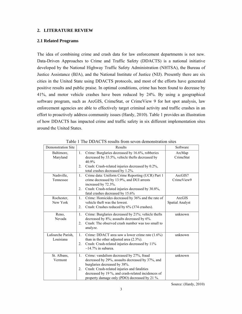
effort to proactively address community issues (Hardy, 2010). Table 1 provides an illustration
of how DDACTS has impacted crime and traffic safety in six different implementation sites
around the United States.
Table 1 The DDACTS results from seven demonstration sites Demonstration Site Results Software
Baltimore, Maryland
1. Crime: Burglaries decreased by 16.6%, robberies decreased by 33.5%, vehicle thefts decreased by 40.9%
2. Crash: Crash-related injuries decreased by 0.2%, total crashes decreased by 1.2%.
ArcMap CrimeStat
Nashville, Tennessee
1. Crime data: Uniform Crime Reporting (UCR) Part 1 crime decreased by 13.9%, and DUI arrests increased by 72.3%.
2. Crash: Crash-related injuries decreased by 30.8%, fatal crashes decreased by 15.6%
ArcGIS7 CrimeView9
Rochester, New York
1. Crime: Homicides decreased by 36% and the rate of vehicle theft was the lowest.
2. Crash: Crashes reduced by 6% (374 crashes).
ArcGIS Spatial Analyst
Reno, Nevada
1. Crime: Burglaries decreased by 21%; vehicle thefts decreased by 8%; assaults decreased by 6%.
2. Crash: The observed crash number was too small to analyze.
unknown
Lafourche Parish, Louisiana
1. Crime: DDACT area saw a lower crime rate (1.6%) than in the other adjusted area (2.3%).
2. Crash: Crash-related injuries decreased by 11% ~14.7% in subarea.
unknown
St. Albans, Vermont
1. Crime: vandalism decreased by 27%, fraud decreased by 29%, assaults decreased by 37%, and burglaries decreased by 38%.
2. Crash: Crash-related injuries and fatalities decreased by 19 %, and crash-related incidences of property damage only (PDO) decreased by 21 %.
unknown
Source: (Hardy, 2010)
4
While DDACTS principles appear to provide impressive results, researchers found that
exaggerated study areas and a naïve before/after evaluation method may lead to bias
regarding the estimation of the program’s true effectiveness.
1. Exaggerated study area: In some community sites, crime and crash data are summarized
at the city or county level instead of using actual DDACTS data ranges. Exaggerated
study areas may bias the estimation of the DDACTS program’s effectiveness because of
miscellaneous unrelated external variables. For example, if the study area is close to the
DDACTS application area, a true estimation of DDACTS’s effectiveness should be close
to the real value. However, if the city boundary is chosen as a data collection range in
comparison with the DDACTS application area the effectiveness value may be skewed.
2. Using a Naïve Before-After Method: The six study reports all used a naïve before-after
evaluation method. This method compare the crash frequency between the before and
after periods only, and it may overestimate treatment’s effects because of site-selection
bias (Hauer, 1997). A more robust method for estimating the effectiveness of DDACTS
as a public safety countermeasure would be to use the empirical Bayesian (EB) method or
a Control Group (CG) method to analyze crash data. In addition, using a naïve before-
after method can only be examined using the Wilcoxon test, which makes limited
quantitative statements about the differences between two non-normal distribution
populations. In other words, the Wilcoxon test cannot show the effective size difference,
and there is no confidence interval for the estimated difference.
Results from current case study reports appear to be positive; however, their estimations of
DDACTS’s effectiveness are limited because of the exaggerated study areas and
inappropriate before-after evaluation methods. Care should be taken when interpreting
previous study results as the reference values. Sensitivity analysis should be used to estimate
the possible benefit of using DDACTS as a means of reducing crime and vehicular crashes.
2.2 Place-Based Theorem
Ronald (2010) noted that B.F. Skinner’s theory of learning explains why crimes and crashes
may occur in the same neighborhood even if there is no causal link between these two events
themselves. According to the DDACTS guidelines, law enforcement agencies perform high
visibility traffic enforcement in their patrol routes that can reduce crimes and crashes. High
visibility traffic enforcement works because of a general deterrent effect. Most people who
fear arrest or detection will drive slower and more carefully. Due to the increased visible
presence of traffic enforcement, criminals may also avoid any illegal activity within these
zones for fear of being arrested.
5
Locations where crashes and crimes occur need to be in close proximity to each other
otherwise high visibility traffic enforcement cannot work efficiently. When crashes and
crimes are distributed randomly or the hot spots are farther from each other, DDACTS
methods are not as effective.
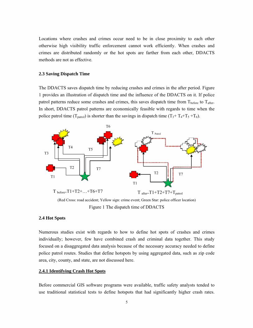
2.3 Saving Dispatch Time
The DDACTS saves dispatch time by reducing crashes and crimes in the after period. Figure
1 provides an illustration of dispatch time and the influence of the DDACTS on it. If police
patrol patterns reduce some crashes and crimes, this saves dispatch time from Tbefore to Tafter.
In short, DDACTS patrol patterns are economically feasible with regards to time when the
police patrol time (Tpatrol) is shorter than the savings in dispatch time (T3+ T4+T5 +T6).
(Red Cross: road accident; Yellow sign: crime event; Green Star: police officer location)
Figure 1 The dispatch time of DDACTS
2.4 Hot Spots
Numerous studies exist with regards to how to define hot spots of crashes and crimes
individually; however, few have combined crash and criminal data together. This study
focused on a disaggregated data analysis because of the necessary accuracy needed to define
police patrol routes. Studies that define hotspots by using aggregated data, such as zip code
area, city, county, and state, are not discussed here.
2.4.1 Identifying Crash Hot Spots
Before commercial GIS software programs were available, traffic safety analysts tended to
use traditional statistical tests to define hotspots that had significantly higher crash rates.
T before=T1+T2+…+T6+T7 T after=T1+T2+T7+Tpatrol
T1
T7
T4 T5
T2
T1
T7
T2
T3
T6
T Patrol
6
Using the traditional statistical method is inconvenient and inefficient, because traffic
engineers must separate road networks into multiple segments with equal lengths (if
possible), record crashes for each segment length, use older statistical methods (such as Chi-
square test) to define hot spots, and show results via tabulated data. In addition, using
traditional statistical methods will not show a geographical relationship between crashes and
other environmental variables.
GIS software programs simplify this procedure and solve problems by providing graphical
data points that can be used for mapping. They have remained one of the most popular tools
for visualization of crash data and hot-spot analysis. Schneider et al. (2004) provided an
excellent review of the methods, findings, and problems related to using GIS for traffic
safety. Previously, some crash datasets were recorded in textual or tabular formats. These
data sets were required to be transformed into geographic data before using GIS software
programs.
1. Traditional numerical methods and GIS spatial methods
Repeatability analysis is common in numerical methods, while Kernel Density Analysis
and Getis-Ord Gi Analysis are common in the GIS spatial method. In repeated analysis,
hot spots were defined as the locations where the top 5% and 1% of crashes occurred. The
crashes for each site were assumed to follow a Poisson distribution with mean crash rate,
λ, which is estimated by dividing the total number of crashes in a given study area by the
segment number. The probability of each site having x number of crashes, P(x), can be
shown as follows,
!)(
x
exP
x (1)
In other words, if a site has more than X95% or X99% crashes, the site was labeled as a
hotspot.
As for the Kernel Density method, it is easy to calculate the risk density for each crash
instead of showing the actual location of each crash. For a site to be considered a hot spot,
it needed to show a crash rate higher than the threshold value. Erdogan et al. (2008) used
the above methods to define crash hot spots in Afyonkarahisar, Turkey, and compared
their differences. The results suggested that repeatability analysis identified more hot
spots than the Kernel Density analysis, but it did not provide the possible reason for
explaining the difference. In a recent study, Gundogdu (2010) also combined traditional
7
numerical methods and Getis-Ord Gi analysis to examine hotspots in Konya, Turkey. Hot
spots were defined as those sites having either the highest 5% crash frequency or the Gi
value. The results showed that using two comparative methods can improve the accuracy
of identifying hotspots.
2. Initial Setting for the Kernel Density Estimation (KDE) method
Compared to more simple evaluation methods, the kernel density method is an advanced
process because it determines the expansion of crash risk, and an arbitrary spatial unit can
be defined for the whole study area for comparison purposes. However, two important
factors will affect the outcome of the KDE: bandwidth and cell size. Anderson (2009)
provided details for setting up the initial settings when the KDE is used to identify crash
hot spots and their cluster patterns. The bandwidth size range is subjective and the value
of the bandwidth and cell size may be adjusted using other conditions, such as the study
area or data.
2.4.2 Crime Hot Spots
The theoretical work for defining hot spots in criminal activity is more complex than that for
traffic study areas, and crime analysis software applications have been previously developed.
Besides ArcGIS, common software packages for crime data collection include CrimeStat,
Spatial Analysis, HotSpot Detective, Vertical Mapper, Crime View, and SpaceStat (Erdogan
et al., 2008; Schneider et al., 2004). Most geographical profiling software packages are used
for analyzing serious crimes committed, or are for analyzing several crime location sites
linked to similar criminal characteristics. While crime and crash incidents are committed by
different people, this study chose to use ArcGIS for the analysis.
2.5 Summary
While a majority of the DDACTS studies focused on the reduction of crime and crash rates
after applying modified patrol routes, this study focused on the change and/or improvement
of police dispatch time. There is no step-by-step procedure of data analysis that can calculate
the change in dispatch times in the literature. The motivation of this study is to examine the
amount of dispatch time that can be saved by applying DDACTS principles. Since there are
no appropriate study results that can be used as a baseline of effectiveness for DDACTS, a
sensitive analysis will be used. Traditional methods (frequency analysis) and geographical
methods (KDE) will both be used for identifying hot spots. Average Nearest Neighbor
(ANN) and Getis-Ord General G will be used for a clustered pattern. All the analyses were
conducted in ArcGIS.
8
3. DATA AND METHODOLOGY
The study area is limited by the service area of the College Station Police Department. Data
were taken from the time period of January 2005 to September 2010. All crime and crash
data were provided by the College station Police Department (CSPD). There were 65,461
crime offense reports, and 14,712 crash reports. The road shape file, “All line Data,” was
downloaded from the Census Bureau's MAF/TIGER database website. The Coordination
System was the GCS North America 1983.
The procedure can be separated as four steps: (1) Geocoding data; (2) Defining hot spots; (3)
Organizing best patrol routes; and, (4) Estimating effectiveness. The following paragraphs
present the characteristics for each step.
3.1 Data Geocoding
The first step, geocoding, consists of transferring according to address information crash and
crime data from a tabulate format to a geographic format. The first matching rates of crimes
and crashes are only about 70%, because datasets use abbreviation and alternative names to
record crashes and crime. Hence, the researchers rewrote the original name from
abbreviations and added the alternative road names in the address locator. The rematch rates
for the crime and crash date increased to 90%.
3.2 Defining Hot Spots
The second stage seeks to determine the location of the hot spots based on the crime and
crash data. This study used three steps to define hotspots more accurately. The first step
involved examining whether data were clustered or not. If crimes and crashes happen
randomly without showing patterns, then high-visibility traffic enforcement may not work,
since there are no defined hotspots to focus upon. We summarized the frequency of each
crime and crash because of data-point overlapping. The actual frequency can be used for
further statistical analyses. Finally, drawing the kernel density surface shows the continuous
possibility of crimes and crashes in the study area. Hot spots can be easily identified by the
color area with high KDE values.
3.2.1 Cluster Index
Average Nearest Neighbor (ANN) and Getis-Ord General G (Gi) are two main methods that
can be used for checking whether crimes and crashes are clustered or not, and the following
sections introduce the theorems and equations to apply those methods.
9
3.2.1.1 Average Nearest Neighbor (ANN)
ANN is a nearest neighbor index based on the average distance from each point to its nearest
neighboring point. Equation (2) shows the calculation for the ANN.
nA
ddANN
/5.0
(2)
Where,
d : The average nearest neighbor distance;
: The average random distance;
A: The area of the study region; and,
n: The number of points.
If the ANN is less than 1, the data contain a clustered point. However, the ANN value can
only be interpreted when the Z-score is significant. If the Z-score is not significant, the ANN
value means nothing because it might occur by random chance.
3.2.1.2 Getis-Ord General G (Gi)
The Getis-Ord General G (Gi) can measure the concentration ratio of high or low values for
the study area. Large Z values (positive, such as +100) mean hot spots clustered together,
while low Z values (negative, such as -100) indicate cold spots clustered together. Equations
(3) to (5) show the calculation for the Gi and Z values.
( )( ) j
j i ji
i ji j
W d X XGi d
X X
(3)
))((
))(()())((
dGiVar
dGiEdGidGiZ
(4)
)1())((
NN
WdGiE (5)
Where,
Gi(d): The Gi value of distance d;
Wj(d): One, when d is less than the threshold value, otherwise is zero;
Xi, Xj: The frequency at location i and j;
Z(Gi(d)): The z value of Gi(d);
E (Gi (d)): The expected value of Gi (d);
10
W: The sum of weight of all pair points; and,
N: The number of the points.
This study used this index only to show the cluster patterns for the crime and crash data, but
further studies could use Gi to compare the different types of crime (robbery, DWI, gun-
related), and different time periods (day and night, weekday and weekend).
3.2.1 Calculating Frequency
The problem of point overlapping causes difficulties in recognizing hot spots by observing
point maps, especially for the high point-density areas. For solving this overlapping problem,
we used the “Collect Event” function to calculate the frequency for each cell. The results
generated new maps that have points with different radii. Points with large radii represent
higher frequencies.
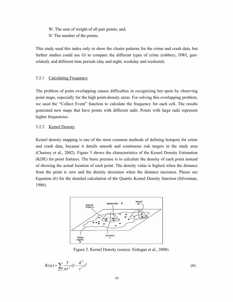
3.2.2 Kernel Density
Kernel density mapping is one of the most common methods of defining hotspots for crime
and crash data, because it details smooth and continuous risk targets in the study area
(Chainey et al., 2002). Figure 5 shows the characteristics of the Kernel Density Estimation
(KDE) for point features. The basic premise is to calculate the density of each point instead
of showing the actual location of each point. The density value is highest when the distance
from the point is zero and the density decreases when the distance increases. Please see
Equation (6) for the detailed calculation of the Quartic Kernel Density function (Silverman,
1986).
Figure 2. Kernel Density (source: Erdogan et al., 2008)
d
duK 2
2
2
2)1(
3)( (6)
11
Where,
K: Kernel density value;
d: The distance from event; and,
τ: Bandwidth.
3.3 Optimum Route
For organizing the best patrol route, another ArcGIS extension, “Network analysis,” was used
to build the best route to connect hot spots via using the shortest distance. Detailed street data
were used to build the network database, and then the Top 5 and Top 10 hotspots were
assigned as the necessary stops for two patrol routes. This study defined the hotspots as the
coincident hot area in the frequency and KDE maps.
3.4 Estimating the Effectiveness
The effectiveness of applying a new police patrol route is estimated by calculating the
difference between the dispatch time in the before and after time periods (see Equation 7).
However, two assumptions were made for convenience of calculation and due to data
limitations:
Based on a neutral assumption, crime and crash rates are reduced by 50% in the effect
area (within a patrol route of 500 feet) in the after period. Since current studies cannot
provide precise estimations as to the effectiveness and the effect area, a sensitivity
analysis needs to be performed to better estimate different scenarios. The effectiveness
varied between a reduction of 25% to up to 75%, and the effect area changed between
250 and 1,000 feet.
The average dispatch time to each point - crime or crash - in the before period and in the
after period is the same. Hence, the calculation using Equation (7) is based on the
frequency of crimes and crashes. The reason why this assumption was used was to
minimize the converging or optimizing time. If we calculate the actual dispatch time for
all the points, this will significantly increase the converging time due to the very large
dataset in ArcGIS.
It should be noted that previous studies assumed the same effectiveness for the whole study
area; however, in this study, we hypothesized that a police patrol route only works in the
effect area. In other words, the crime and crash rate will not change outside the effect area,
because the visibility of highly visible law enforcement decreases when the distance
increases.
12
n m
j, after i, beforej i j, after i, before
j, after i, beforemi, before
i, beforei
T - Tn T -m T n-m
(%) = ( T T )m T mT
(7)
Where,
θ : The Effectiveness of new police patrol route;
Ti,before, Ti,after : The dispatch time to point i in the before and after periods;
M: The number of events in the before period; and,
n: The number of events in the after period.
4. APPLICATION, RESULTS AND DISCUSSION
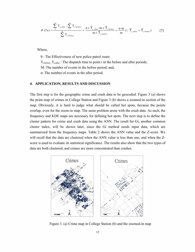
The first step is for the geographic crime and crash data to be geocoded. Figure 3 (a) shows
the point map of crimes in College Station and Figure 3 (b) shows a zoomed-in section of the
map. Obviously, it is hard to judge what should be called hot spots, because the points
overlap, even for the zoom-in map. The same problem arose with the crash data. As such, the
frequency and KDE maps are necessary for defining hot spots. The next step is to define the
cluster pattern for crime and crash data using the ANN. The result for Gi, another common
cluster index, will be shown later, since the Gi method needs input data, which are
summarized from the frequency maps. Table 2 shows the ANN value and the Z-score. We
will recall that the data are clustered when the ANN value is less than one, and when the Z-
score is used to evaluate its statistical significance. The results also show that the two types of
data are both clustered, and crimes are more concentrated than crashes.
Figure 3. (a) Crime map in College Station (b) and the zoomed-in map
13
Table 2. ANN value of crash and crime data in College Station ANN (NNR, Z)
Crash Cluster (0.08, -198.5) Crime Cluster (0.05, -455.8)
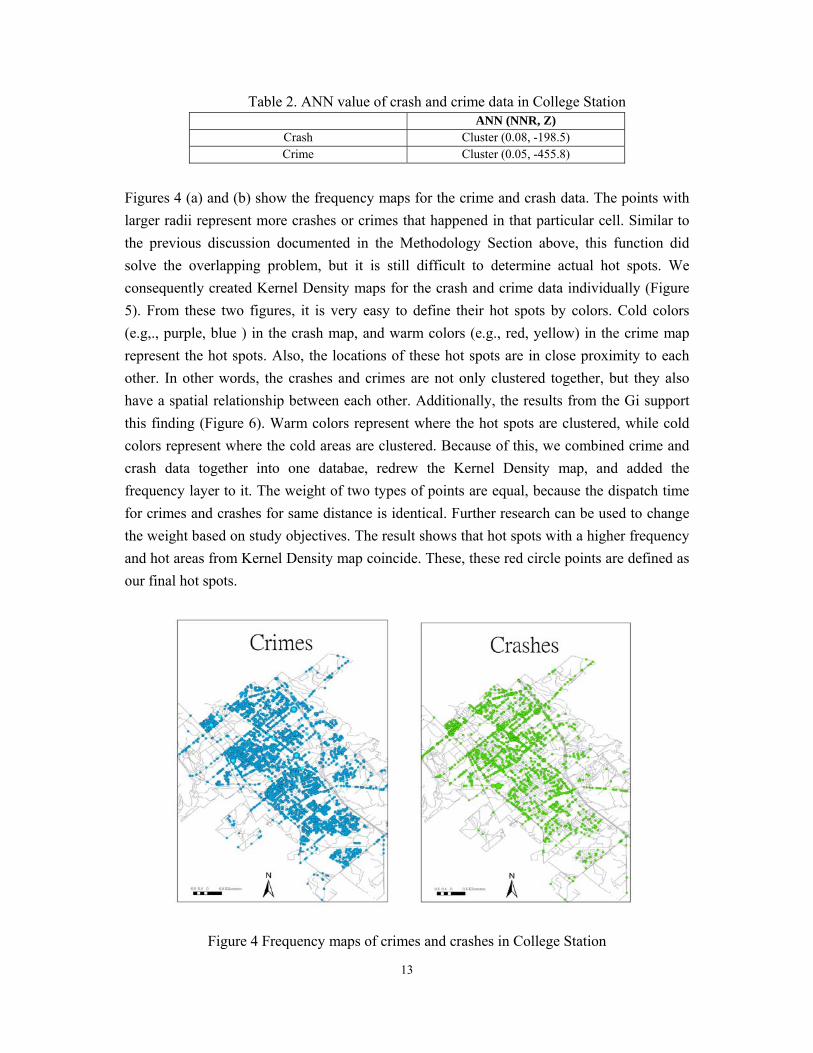
Figures 4 (a) and (b) show the frequency maps for the crime and crash data. The points with
larger radii represent more crashes or crimes that happened in that particular cell. Similar to
the previous discussion documented in the Methodology Section above, this function did
solve the overlapping problem, but it is still difficult to determine actual hot spots. We
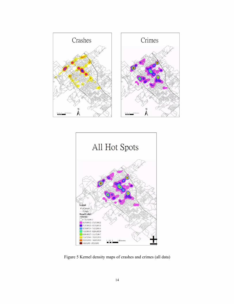
consequently created Kernel Density maps for the crash and crime data individually (Figure
5). From these two figures, it is very easy to define their hot spots by colors. Cold colors
(e.g,., purple, blue ) in the crash map, and warm colors (e.g., red, yellow) in the crime map
represent the hot spots. Also, the locations of these hot spots are in close proximity to each
other. In other words, the crashes and crimes are not only clustered together, but they also
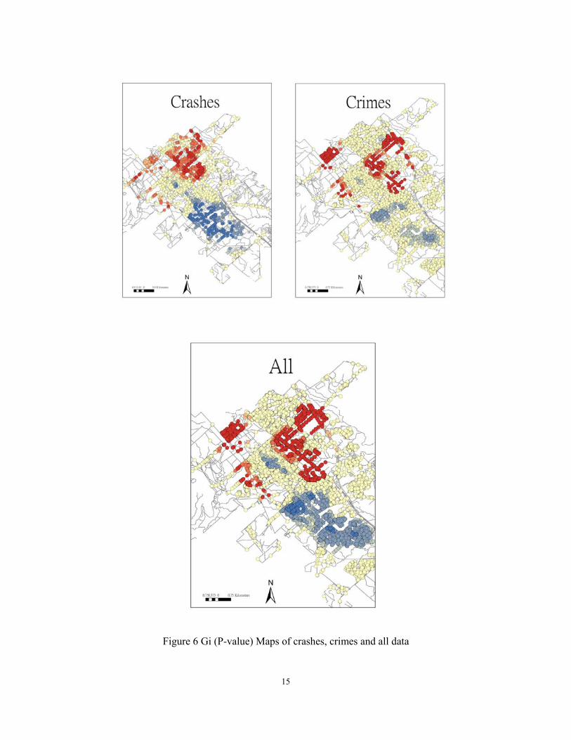
have a spatial relationship between each other. Additionally, the results from the Gi support
this finding (Figure 6). Warm colors represent where the hot spots are clustered, while cold
colors represent where the cold areas are clustered. Because of this, we combined crime and
crash data together into one databae, redrew the Kernel Density map, and added the
frequency layer to it. The weight of two types of points are equal, because the dispatch time
for crimes and crashes for same distance is identical. Further research can be used to change
the weight based on study objectives. The result shows that hot spots with a higher frequency
and hot areas from Kernel Density map coincide. These, these red circle points are defined as
our final hot spots.
Figure 4 Frequency maps of crimes and crashes in College Station
14
Figure 5 Kernel density maps of crashes and crimes (all data)
15
Figure 6 Gi (P-value) Maps of crashes, crimes and all data
16
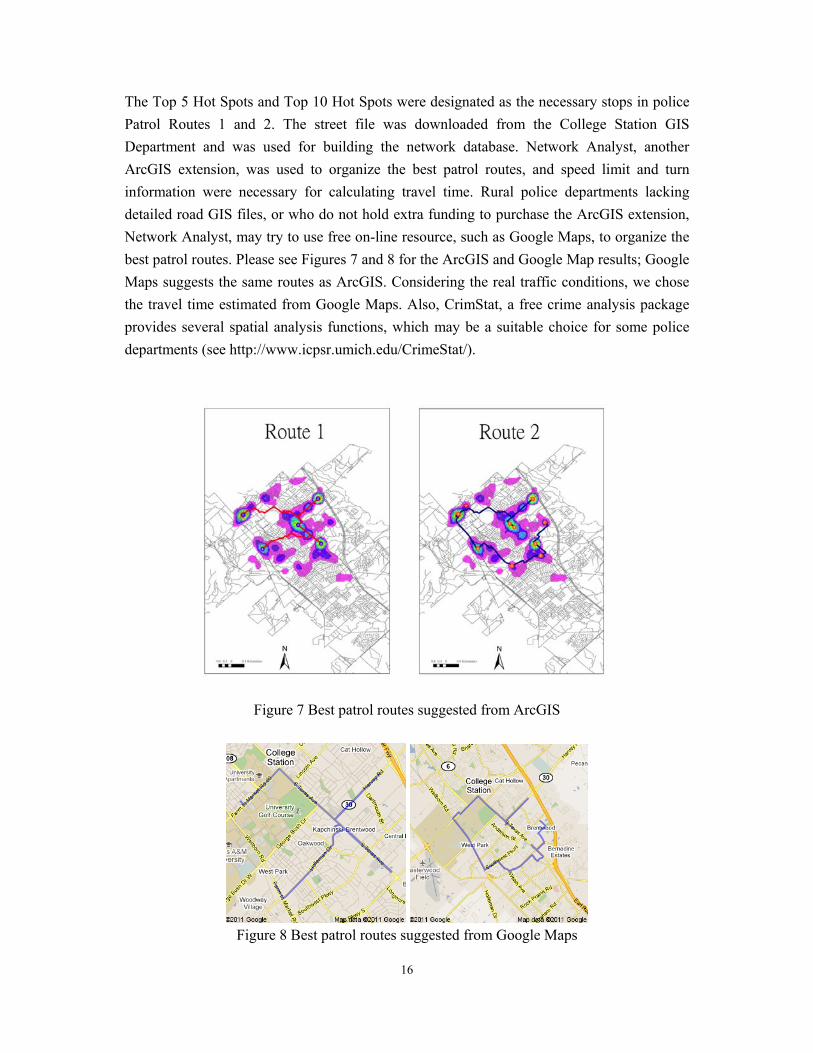
The Top 5 Hot Spots and Top 10 Hot Spots were designated as the necessary stops in police
Patrol Routes 1 and 2. The street file was downloaded from the College Station GIS
Department and was used for building the network database. Network Analyst, another
ArcGIS extension, was used to organize the best patrol routes, and speed limit and turn
information were necessary for calculating travel time. Rural police departments lacking
detailed road GIS files, or who do not hold extra funding to purchase the ArcGIS extension,
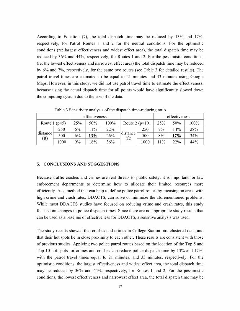
Network Analyst, may try to use free on-line resource, such as Google Maps, to organize the
best patrol routes. Please see Figures 7 and 8 for the ArcGIS and Google Map results; Google
Maps suggests the same routes as ArcGIS. Considering the real traffic conditions, we chose
the travel time estimated from Google Maps. Also, CrimStat, a free crime analysis package
provides several spatial analysis functions, which may be a suitable choice for some police
departments (see http://www.icpsr.umich.edu/CrimeStat/).
Figure 7 Best patrol routes suggested from ArcGIS
Figure 8 Best patrol routes suggested from Google Maps
17
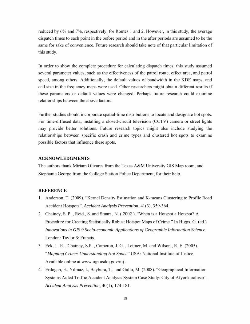
According to Equation (7), the total dispatch time may be reduced by 13% and 17%,
respectively, for Patrol Routes 1 and 2 for the neutral conditions. For the optimistic
conditions (re: largest effectiveness and widest effect area), the total dispatch time may be
reduced by 36% and 44%, respectively, for Routes 1 and 2. For the pessimistic conditions,
(re: the lowest effectiveness and narrowest effect area) the total dispatch time may be reduced
by 6% and 7%, respectively, for the same two routes (see Table 3 for detailed results). The
patrol travel times are estimated to be equal to 21 minutes and 33 minutes using Google
Maps. However, in this study, we did not use patrol travel time to estimate the effectiveness,
because using the actual dispatch time for all points would have significantly slowed down
the computing system due to the size of the data.
Table 3 Sensitivity analysis of the dispatch time-reducing ratio
effectiveness effectiveness
Route 1 (p=5) 25% 50% 100% Route 2 (p=10) 25% 50% 100%
distance (ft)
250 6% 11% 22% distance
(ft)
250 7% 14% 28%
500 6% 13% 26% 500 8% 17% 34%
1000 9% 18% 36% 1000 11% 22% 44%
5. CONCLUSIONS AND SUGGESTIONS
Because traffic crashes and crimes are real threats to public safety, it is important for law
enforcement departments to determine how to allocate their limited resources more
efficiently. As a method that can help to define police patrol routes by focusing on areas with
high crime and crash rates, DDACTS, can solve or minimize the aforementioned problems.
While most DDACTS studies have focused on reducing crime and crash rates, this study
focused on changes in police dispatch times. Since there are no appropriate study results that
can be used as a baseline of effectiveness for DDACTS, a sensitive analysis was used.
The study results showed that crashes and crimes in College Station are clustered data, and
that their hot spots lie in close proximity to each other. These results are consistent with those
of previous studies. Applying two police patrol routes based on the location of the Top 5 and
Top 10 hot spots for crimes and crashes can reduce police dispatch time by 13% and 17%,
with the patrol travel times equal to 21 minutes, and 33 minutes, respectively. For the
optimistic conditions, the largest effectiveness and widest effect area, the total dispatch time
may be reduced by 36% and 44%, respectively, for Routes 1 and 2. For the pessimistic
conditions, the lowest effectiveness and narrowest effect area, the total dispatch time may be
18
reduced by 6% and 7%, respectively, for Routes 1 and 2. However, in this study, the average
dispatch times to each point in the before period and in the after periods are assumed to be the
same for sake of convenience. Future research should take note of that particular limitation of
this study.
In order to show the complete procedure for calculating dispatch times, this study assumed
several parameter values, such as the effectiveness of the patrol route, effect area, and patrol
speed, among others. Additionally, the default values of bandwidth in the KDE maps, and
cell size in the frequency maps were used. Other researchers might obtain different results if
these parameters or default values were changed. Perhaps future research could examine
relationships between the above factors.
Further studies should incorporate spatial-time distributions to locate and designate hot spots.
For time-diffused data, installing a closed-circuit television (CCTV) camera or street lights
may provide better solutions. Future research topics might also include studying the
relationships between specific crash and crime types and clustered hot spots to examine
possible factors that influence these spots.
ACKNOWLEDGMENTS
The authors thank Miriam Olivares from the Texas A&M University GIS Map room, and
Stephanie George from the College Station Police Department, for their help.
REFERENCE
1. Anderson, T. (2009). “Kernel Density Estimation and K-means Clustering to Profile Road
Accident Hotspots”, Accident Analysis Prevention, 41(3), 359-364.
2. Chainey, S. P. , Reid , S. and Stuart , N. ( 2002 ). “When is a Hotspot a Hotspot? A
Procedure for Creating Statistically Robust Hotspot Maps of Crime.” In Higgs, G. (ed.)
Innovations in GIS 9 Socio-economic Applications of Geographic Information Science.
London: Taylor & Francis.
3. Eck, J . E. , Chainey, S.P. , Cameron, J. G. , Leitner, M. and Wilson , R. E. (2005).
“Mapping Crime: Understanding Hot Spots.” USA: National Institute of Justice.
Available online at www.ojp.usdoj.gov/nij .
4. Erdogan, E., Yilmaz, I., Baybura, T., and Gullu, M. (2008). “Geographical Information
Systems Aided Traffic Accident Analysis System Case Study: City of Afyonkarahisar”,
Accident Analysis Prevention, 40(1), 174-181.
19
5. Federal Bureau of Investigation, FBI,
http://www2.fbi.gov/ucr/cius2009/data/table_01.html(May. 11, 2011).
http://www.fbi.gov/news/pressrel/press-releases/fbi-releases-2009-crime-statistics
6. Gundogdu, I. B. (2010). “Applying Linear Analysis Methods to GIS-supported
Procedures for Preventing Traffic Accidents: Case Study of Konya”, Safety Science,
48(6), 763-769.
7. Hardy E. (2010). “Data-Driven Policing: How Geographic Analysis Can Reduce Social
Harm”, Geography Public Safety, 2(3).
8. Hauer, E. (1997). Observational Before-After Studies in Road Safety. Pergamon
Publications, London.
9. Loo, B. P. Y. (2006). “Validating Crash Locations for Quantitative Spatial Analysis: A
GIS-based Approach”, Accident Analysis Prevention, 38(5), 879-886.
10. National Highway Traffic Safety Administration (NHTSA) website, http://www-
nrd.nhtsa.dot.gov/Pubs/811363.pdf (May. 11, 2011).
11. Schneider, R.J., Ryznar, R.M., Khattak, A.J. (2004). “An Accident Waiting To Happen:
A Spatial Approach To proactive Pedestrian Planning”, Accident Analysis Prevention,
36(3):193-21.
12. Silverman B. (1986). Density Estimation for Statistics and Data Analysis, London:
Chapman and Hall.
13. Wilson R. E. (2010). “Place as the Focal Point: Developing a Theory for the DDACTS
Model”, Geography Public Safety, 2(3).
14. Weiss A. and Morckel, C. K. (2007). “Strategic and Tactical Approaches to Traffic
Safety”, The Police Chief, 74 (7).


![[Kuo-Yann Lai] Liquid Detergents(BookZZ.org)](https://img.pdfslide.us/doc/110x75/55cf969b550346d0338ca125/kuo-yann-lai-liquid-detergentsbookzzorg.jpg)