Using GANDALF via Python

Giovanni Rosotti

IoA Cambridge

28th October 2015

Why?

• As a user, you will probably spend more time analysing simulations rather than coding the algorithms

• So we should provide you with the right tools

Can’t I use SPLASH?

• Yes you can! SPLASH is a very advanced tool

• But…

• data is very difficult (if not impossible) to access programmatically

• interface is not exactly user friendly…

Basic design principle

• Be transparent

• Make programmatically accessible all data to you, the user. You can call functions to do the same things the plotting functions do

• This means, anything you can plot you can also save in a variable

What can you do?

• Set-up and run a simulation (today only basics; more tomorrow)

• Read in an existing simulation

• Do “standard” plots (particle and rendered plots)

• Create and plot user-defined quantities

• Save standard and user-defined quantities in variables to do what you want with them

• Plot quantities as a function of time

How to use the library

• inside a python script (works from every folder):

• using the simple interpreter (from the gandalf folder):

For all of this to work you need to set correctly the PYTHONPATH variable (see userguide)

from gandalf.analysis.facade import *

python analysis/gandalf_interpreter.py

export PYTHONPATH=$PYTHONPATH:folder_containing_gandalf_folder

Interpreter

• If you want to do something very quick, you can use the interpreter (it saves you from typing a few characters)

• No parenthesis and commas needed

• Loosely inspired by GNUPLOT. Built using the library cmd2 (https://pythonhosted.org/cmd2/)

• The command help prints all the supported commands

• help command gives information about a command

• Limitation: the only thing you are allowed to do is calling functions defined in facade

A basic example

This will be done using the interpreter

From now on we move to using normal Python scripts. If you want to use the interpreter the conversion is trivial

newsim tests/adsod.dat

setupsim

plot x rho

run

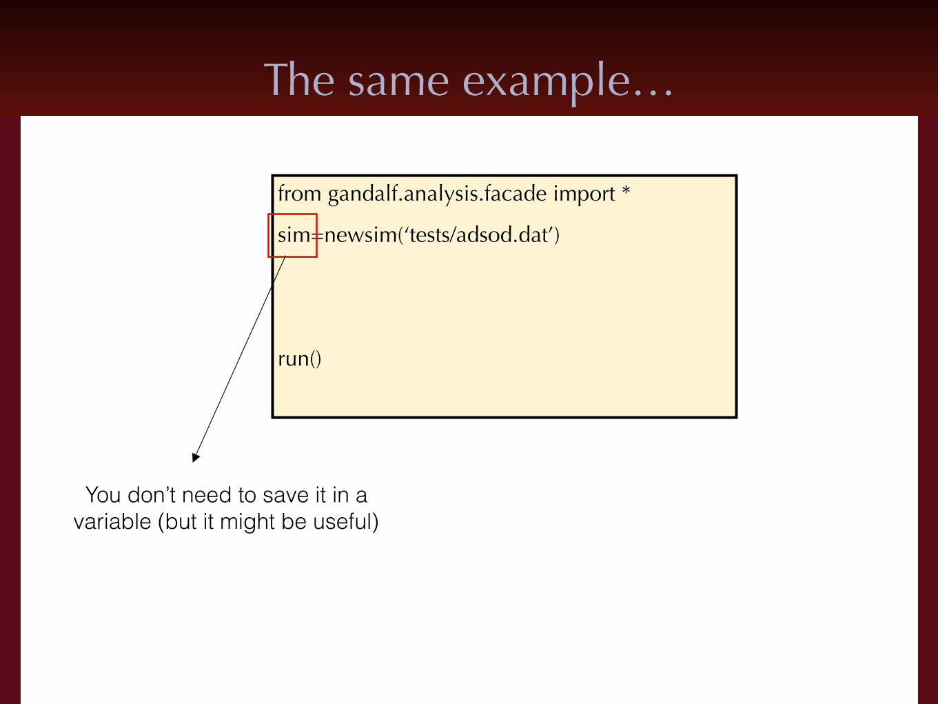
The same example…

You don’t need to save it in a variable (but it might be useful)

from gandalf.analysis.facade import *

sim=newsim(‘tests/adsod.dat’)

run()

Tells GANDALF that you have finished setting-up the simulation You can still modify the parameters via python - will be covered in a separate tutorial

The same example…

from gandalf.analysis.facade import *

sim=newsim(‘tests/adsod.dat’)

setupsim()

plot(‘x’,’rho’)

run()

Look at what happens to the plot after you type this!

Jumping between snapshots

• If now you want to go back to the first snapshot, just type:

• You can also use the convenience functions next() and previous()

• This updates the plot

• snap uses python indexing (i.e. -1 is the last snapshot)

snap(0)

And if I want to compare two different snapshots?

• Just do the following:

• In this case the plots will NOT be updated when you call the function snap

• By default plots are tied to the CURRENT snapshot

These two are the same (default behaviour is that plot REPLACES what

is on the plot)

plot(‘x’,’rho’,snap=0)

addplot(‘x’,’rho’,snap=1)

plot(‘x’,’rho’,snap=1,overplot=True)

Cool. And if I want to compare two different SIMULATIONS?

loadsim(‘ADSOD1’)

snap(-1)

plot(‘x’,’rho’)

loadsim(‘ADSOD2’)

snap(-1)

addplot(‘x’,’rho’)

• Plots by default are tied to the current simulation

• Creating a new simulation or loading an existing one changes the current simulation

That was cheating… what if I want to go back to a previous simulation?

plot(‘x’,’rho’,sim=0,snap=0)

addplot(‘x’,’rho’,sim=1,snap=1)• You might also find useful the following functions:

set_current_sim(1)

sims()

snaps(0)

These two functions output informations about the simulations loaded in memory and their snapshots

Fine, but it was a bit boring. Show me more pretty pictures!

• I take it you want to see some colours. Ok, let’s introduce rendered plots then

newsim(‘tests/khi.dat’)

setupsim()

render(‘x’,’y’,’rho’)

run()

And in 3d?

3d defaults to projection; if you want a slice you need to specify it

newsim(‘tests/bossbodenheimer.dat’)

setupsim()

render(‘x’,’y’,’rho’,zslice=0)

run()

Other types

newsim(‘tests/bossbodenheimer.dat’)

setupsim()

render(‘x’,’y’,’rho’,zslice=0)

addplot(‘x’,’y’,type=‘star’)

run()

“Computational Astrophysics with GANDALF” - Freising, Bavaria, 26th - 30th October 2015

Units

• All plotting functions also support units

• Just pass the unit you like and GANDALF will rescale it automatically

loadsim(‘BB1’)

plot(‘x’,’y’,xunit=‘au’,yunit=‘pc’)

Outputting to files

• You can use the button to save a figure in a file

• However it’s useful to be able to do it also from the script itself (for example if you just want to run a script)

• Use the savefig function

• We also provide a make_movie function if you want to create a movie

Quantities

• As you might have guessed ‘x’ and ‘rho’ are expressions that the library understands

• To add a new quantity use:

• If you want to know which quantities are defined, call the KnownQuantities function (will be pushed as soon as internet starts working again)

• The code itself uses this function to define many quantities (e.g. cylindrical/spherical coordinates, pressure, …)

Tells GANDALF that your quantity has the same dimensions as the existing quantity ‘x’

CreateUserQuantity(‘myquantity’,’x+y’,scaling_factor=‘x’)

Quantities - more complicated

• you can also provide your own function

CreateUserQuantity(‘myquantity’,myfunction,scaling_factor=‘x’)

• Here my function is a python function which is called in the following way:

myfunction(snap,type=“default”, unit=“default")

These are the same parameters that you can pass to get_data for example: x=get_data(‘x’,type=type,snap=snap,unit=unit)

Save in x the array with the x coordinates of all particles. You will probably need this function to implement myfunction!

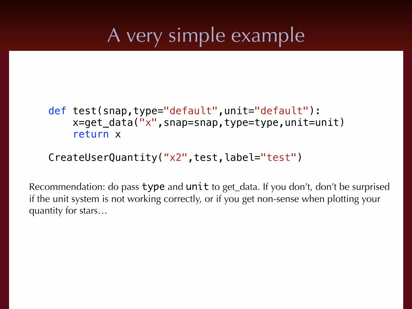
Recommendation: do pass type and unit to get_data. If you don’t, don’t be surprised if the unit system is not working correctly, or if you get non-sense when plotting your quantity for stars…

def test(snap,type="default",unit="default"): x=get_data("x",snap=snap,type=type,unit=unit) return x

CreateUserQuantity(“x2",test,label="test")

A very simple example

Retrieving data

• We just saw the get_data function

• We also provide a get_render_data function in case you want the rendered data. Works like render, but saves the result in a variable instead of plotting. Useful if you want to grid the SPH data (TODO: at the moment actually works only on a 2d grid)

• The plotting functions also return the data they are plotting, in case you want to save it to a variable

• Plotting functions return data through a very simple object (defined in analysis/data.py). You can retrieve the arrays in the following way:

data=plot(‘x’,’y’)

x=data.x_data

y=data.y_data

data=render(‘x’,’y’,’rho’)

render_data=data.render_data

Known limitation: render does not currently return the grid used in x_data and y_data

• Sometimes it’s useful to see how a quantity evolved with time

• This can be monitored using time_plot:

newsim(‘tests/plummer.dat’)

run()

from gandalf.analysis.compute import lagrangian_radii

CreateTimeData(‘lag_0.7’,lagrangian_radii,mfrac=0.7)

time_plot(’t’,’lag_0.7’)

Time plots

This parameter is passed to lagrangian_radii

continued

• Another useful pre-defined function is COM (the center of mass)

• You can also plot quantities for a given particle

• For example plot x coordinate of particle with id 4 as a function of time:

• Bonus: can you use this function also to plot tracks?

• Have a look at example14.py

time_plot(’t’,’x’,id=4,linestyle=‘-‘)

Time plots again

• You can also use your own functions to define a quantity that time_plot understands

• CreateTimeData(name, myfunction)

• Under the hood, the library itself actually uses this function for retrieving the time of a snapshot, for computing lagrangian radii, centre of mass, …

• The function it’s called like this:

myfunction(snap, type=“default”, unit=“default”)

Example

def myfunction(snap,type="default",unit="default"): vx=get_data(“vx”,snap=snap,type=type,unit=unit) m=get_data(“m”,snap=snap,type=type,unit=unit) momentumx=(m*vx).sum() return momentum

CreateTimeData(“momx",myfunction)

Not very different from what we saw before with CreateUserQuantity

The only constraint is that here you have to return a scalar rather than an array

Matplotlib

• Remember we use Matplotlib for plotting

• This means if you are not satisfied you can customise a plot via matplotlib calls

• You can also pass kwargs to the plotting functions, which will be passed to matplotlib

• A very technical note. Python has some known problems with parallelisation. This means that when a simulation is running you cannot interact with the matplotlib plots

• There is a solution which consists in setting parallel to True in the file defaults.py. However this means you will lose the possibility of calling directly matplotlib functions (technical: this happens because the plotting is done in another process). Not too bad as you need it only if you want to do a plot of a simulation which is running (so probably you don’t particularly care about the plot visual appearance)

“Computational Astrophysics with GANDALF” - Freising, Bavaria, 26th - 30th October 2015

More

• If you want to know more, have a look at the examples and/or at the tests

• You can also browse through the code in facade. The functions that you care about are documented (the text you see in the docstring is the same one that gets printed if you type help command in the interpreter)

• The user guide will be expanded in the next weeks

• Do let us know about the bugs you will find!