Using Force Sensing Resistor to Evaluate Lateral Earth Pressure Distribution Between

Closely Spaced Geosynthetic Reinforcements

A Thesis submitted in partial fulfillment of the requirements for the degree of Master of

Science at George Mason University

by

Tshreya Bhattarai

Bachelor’s Degree in Engineering

Tribhuvan University, 2012

Director: Burak F. Tanyu, Associate Professor Department of Civil and Infrastructure Engineering

Fall Semester 2017

George Mason University

Fairfax, VA

ii

Copyright 2017 Tshreya Bhattarai

All Rights Reserved

iii

DEDICATION

This thesis is dedicated to my loving family and my friends for their unconditional

support without whom I would not have made it this far.

iv

ACKNOWLEDGEMENTS

I would like to express my gratitude to my advisor Dr. Burak Tanyu for his invaluable

guidance and support. I am thankful to Mr. Fred C. Chuck from TenCate to provide

Mirafi HP 570 geotextile and Mr. Robert Lozano from Reinforced Earth Company to

provide the customized reinforced concrete panels that were used to create the small-

scale model experiments used in my study. Both products were provided as a support to

the research program without any costs. I greatly appreciate these financial supports. I

would also like to thank Mr. Dave Stiles, who has already completed his master’s degree

in GMU and is a Lieutenant ranking officer at U.S. Coast Guard. He has provided

significant support by volunteering his time to help creating the customized data

acquisition system to obtain data from the sensors I used in my research. This project

would not have come this far without his help. I would like to thank all members of the

Sustainable Goetransportation Infrastructure (SGI) research group for their feedback and

support. Finally, I would like to thank the committee members for my thesis for taking

their precious time and providing feedback.

v

TABLE OF CONTENTS

Page

List of Tables .................................................................................................................... vii

List of Figures .................................................................................................................. viii

Abstract .............................................................................................................................. ix

Chapter One: Introduction .................................................................................................. 1

Chapter Two: Experimental Program ................................................................................. 8

Chapter Three: Materials .................................................................................................. 12

Soils used in SSME measurement ................................................................................. 12

AASHTO No. 8 aggregate ......................................................................................... 12

Sand ........................................................................................................................... 13

Reinforcement geosynthetic .......................................................................................... 15

Earth pressure sensors ................................................................................................... 17

Force sensing resistors (FSR) .................................................................................... 17

Rectangular earth pressure cell (RPC) ....................................................................... 19

Chapter Four: Data Collection .......................................................................................... 20

Data Acquisition System (DAQ) for force sensing resistor .......................................... 20

Data Acquisition System for rectangular pressure cell ................................................. 21

Chapter Five: Calibration of Instruments ......................................................................... 22

Calibration of rectangular pressure cell ........................................................................ 22

Calibration of force sensing resistors ............................................................................ 23

Chapter Six: Result ........................................................................................................... 30

Theoretical lateral pressure distribution behind the facing of SSME ........................... 30

Measured lateral pressure distribution from SSME with AASHTO No. 8 aggregate .. 34

Measured lateral pressure distribution from SSME with sand ...................................... 36

Chapter Seven: Discussion ............................................................................................... 41

Comparison of SSME results from AASHTO No. 8 aggregate with theoretical pressure

distribution .................................................................................................................... 41

vi

Comparison of SSME result with theoretical pressure distribution for sand ................ 44

Chapter Eight: Practical Implications, Conclusions, and Limitations .............................. 48

Appendix A: Characterization of Soil ............................................................................... 51

AASHTO No. 8: ............................................................................................................ 52

Optimum unit weight ................................................................................................. 52

Consolidated drained (CD) triaxial test by ASTM D7181 ........................................ 53

Sand ............................................................................................................................... 53

Minimum Index Density Test and Unit weight of sand. (ASTM D4245-14) ........... 53

Maximum Index Density of soil and Unit weight of sand. (ASTM D4253-14) ....... 56

Relative Density: ....................................................................................................... 60

Consolidated drained (CD) triaxial test by ASTM D7181 ........................................ 62

Appendix B: Calibration of Force sensing Resistor (FSR) ............................................... 63

Calibration of FSR as is ................................................................................................ 64

Calibration of Modified FSR......................................................................................... 73

Appendix C: Vertical Pressure measurements from Modified FSR ................................. 90

Vertical Pressure Measurement ..................................................................................... 91

Appendix D: Hysteresis in FSR ........................................................................................ 97

Hysteresis in FSR .......................................................................................................... 98

Hysteresis of FSR as is: ............................................................................................. 98

Hysteresis of modified FSR:...................................................................................... 99

Appendix E: Background on Design .............................................................................. 102

FHWA Manual Guidelines on Lateral earth pressure ................................................. 103

References ....................................................................................................................... 107

vii

LIST OF TABLES

Table Page

Table 1: Properties of the backfill material used in the experimental program ................ 13 Table 2: Properties of geosynthetics ................................................................................. 15

viii

LIST OF FIGURES

Figure Page

Figure 1: Layout of SSME (a) facing blocks marked for each 0.1 m layer boundary and

(b) with FSR and RPC instrumentation behind the facing blocks ...................................... 9

Figure 2: Connection of reinforcements within SSME layout (a) frictional connection at

0.2 m vertical spacing (b) placement of reinforcement at 0.1 m vertical spacings without

any connection to CMU blocks......................................................................................... 10

Figure 3: Grain Size Distribution of AASHTO No. 8 Aggregate and sand ..................... 14

Figure 4: 25mm thick sand interface in between AASHTO No. 8 aggregate and FSR ... 16 Figure 5: FSR’s (a) internal structure and (b) view from the top ..................................... 18

Figure 6: Dataloggers for (a)FSR and (b) RPC ................................................................ 21 Figure 7: Calibration setup of the (a) RPC and FSR: (b)modification of the sensor and (c)

dead load used for calibration ........................................................................................... 23

Figure 8: Calibration result of (a) RPC with sand and AASHTO No. 8 aggregate and (b)

example of a calibration curve with modified FSR from one sensor ............................... 25

Figure 9: FSR measurement (without the application of factor) compared with at rest

pressure distribution, active pressure distribution and RPC measurement ....................... 26 Figure 10: Stress relaxation of rubber pad over time ........................................................ 28

Figure 11: Theoretical earth pressure distributions, bin pressure distribution and Soong

and Koerner pressure distribution based on 0.2m reinforcement spacing ........................ 33 Figure 12: Lateral stress measurements from FSR sensors placed in SSME from

AASHTO No. 8 aggregate that is (a) unreinforced (no geotextile) (b) reinforced with 0.2

m spaced geotextile, and (c) reinforced with 0.1 m spacing ............................................. 35 Figure 13: Lateral stress measurements from FSR sensors placed in SSME from sand that

is (a) unreinforced (no geotextile) (b) reinforced with 0.2 m spaced geotextile, and (c)

reinforced with 0.1 m spacing. .......................................................................................... 39 Figure 14: Comparison of theoretical lateral pressures computed with lateral pressure

measurements obtained from 0.6 m-thick SSME with AASHTO No. 8 aggregate for all

cases: (a) unreinforced (no geotextile, (b) geotextile spaced at 0.2 m, and (c) geotextile

spaced at 0.1 m. ................................................................................................................. 43

Figure 15: Comparison of theoretical lateral pressures computed with lateral pressure

measurements obtained from 0.6 m-thick SSME with sand aggregate for all cases: (a)

unreinforced (no geotextile, (b) geotextile spaced at 0.2 m, and (c) geotextile spaced at

0.1 m. ................................................................................................................................ 47

ix

ABSTRACT

USING FORCE SENSING RESISTOR TO EVALUATE LATERAL EARTH

PRESSURE DISTRIBUTION BETWEEN CLOSELY SPACED GEOSYNTHETIC

REINFORCEMENTS

Tshreya Bhattarai, M.S.

George Mason University, 2017

Thesis Director: Dr. Burak F. Tanyu

Mechanically stabilized earth (MSE) structures have been in use around the world

for many years and are constructed with a variety of reinforcement types and spacing. In

most applications, the common approach is to construct MSE structures with the largest

reinforcement spacing allowed. However, recently for bridge abutment applications, there

have been many MSE structures constructed with geotextile reinforcements vertically

spaced as low as 100 mm apart. Evaluating the lateral stress distribution between such

closely spaced structures is a challenging task as the conventional instruments to measure

earth pressures take up the entire space in between the reinforcements. The focus of this

research was to evaluate the suitability of using a new instrument referred as force

sensing resistor (FSR) system (only 25.4 by 25.4 mm in size) to evaluate lateral stress

distribution in between closely spaced reinforcements. The research was conducted using

a model scale MSE wall constructed in the laboratory. Results were obtained both with

x

and without reinforcements and compared against the existing theoretical lateral earth

pressure distributions and a data obtained from a commercially available earth pressure

cell. The comparison of the data shows that FSR could be a viable tool to measure lateral

earth pressures in such close spacing

1

CHAPTER ONE: INTRODUCTION

Mechanically stabilized earth (MSE) structures have been in use around the world

for many years and are constructed with a variety of reinforcement types and spacing. In

most applications, the owners seek for design options, where the reinforcements are

placed as far apart from each other as possible within the bounds of what is accepted by

regulations of each Country. This approach is followed primarily to reduce the cost

associated with reinforcements as the higher the spacing between the reinforcements the

lower the costs associated with reinforcements. However, since 2011, with Federal

Highway Administration’s (FHWA) “Every Day Counts” innovations program (Adams

et al. 2011), constructing MSE structures with as low as 0.2 m reinforcement within the

main reinforced body and 0.1 m within the bearing bed also became part of the practice

(Wu et al. 2001; Adams et al. 2011; Blosser et al. 2012; Nicks et al. 2013; Talebi et al.

2014). Although in principle this approach is the opposite of what has been the customary

practice in terms of vertical spacing, based on FHWA’s reports, it is reported that this

approach provides up to 60% cost savings compare the conventional abutment techniques

(Adams et al. 2012). FHWA reports that there are 174 of these structures already

constructed in the U.S. This data shows that unlike the previous approach, modern MSE

structures are now being constructed with variety of vertical spacing ranging from what

would be considered very closely spaced (0.1 m) (Wu et al. 2001; Adams et al. 2011;

2

Blosser et al. 2012; Nicks et al. 2013; Talebi et al. 2014) to much larger spacing (up to 2

m) (Tanyu et al. 2016 and Gu et al. 2017) depending on the application and the associated

design.

The design associated with MSE structures have been around many years and

American Association of State Highway Transportation Officials (AASHTO) as well

Federal Highway Administration (FHWA) already provide detailed design guidelines that

are available through publications (Allen et al. 1992; Allen & Bathurst 2001; Morrison et

al. 2006; Berg et al. 2009). When it comes to designing the facing connections the MSE

walls act as a rigid body. To calculate the internal and external stability of the MSE wall,

Coulomb’s method is used to determine the lateral earth pressure behind the MSE facing

with wall friction angle assumed to be zero. The lateral earth pressure coefficient ratio

Kr/Ka in the MSE wall varies with depth for a different type of geo-reinforcement. This

is based on a simplified method developed to avoid iterative design procedure. For

geosynthetic reinforcement, the value of Kr/Ka is 1 throughout the depth of the MSE

wall, therefore the lateral stress distribution increases linearly with the depth (Berg et al.

2009).

For closely spaced MSE structures one of the primary design components

assumes that the lateral earth pressure behind the facing is relatively constant and is

independent of the height of the wall (Adams et al. 2011). This assumption is based on

what is referred as “bin pressure theory” developed by Wu (2001) where it is believed

that the closely spaced reinforcements restrain the lateral deformation of the soil and

create constant pressure throughout the depth of the wall (Wu 2001; Adams et al. 2011;

3

Wu, et al. 2015). According to Wu (2001), the Rankine earth pressure theory over-

estimates the lateral earth pressure behind the wall and the magnitude of the force behind

the closely reinforced system is a function of reinforced spacing, the shear strength of the

material, and rigidity of facing. In bin pressure theory, the lateral earth pressure behind

the closely spaced system is estimated as σh =kaϒ Sv; where: σh is the horizontal stress,

ka is the active lateral earth pressure coefficient, ϒ is the unit weight of the soil and Sv is

the vertical reinforcement.

According to the theory, in idealized condition, the pressure is zero at the top

reinforcement boundary and the lateral stress increases linearly before rebounding back

to zero at the bottom reinforcement boundary (Adams et al. 2011). In real condition,

however, the reinforcement may deform, and soil-reinforcement interface may not bond

properly leading to a condition where at each interface, the pressure at the top

reinforcement is (1/3) σh which increases linearly before decreasing back to (2/3) σh at

the bottom reinforcement.

The design procedures discussed above have been developed over the years based

on the findings from many laboratory studies and field instrumentations (Wu et al. 2006;

Adams et al. 2011; Blosser et al. 2012; Vennapusa et al. 2012; Budge et al. 2014;

Raghunathan et al. 2014; Warren et al. 2014). As demonstrated in the above design

components, one of the important components of field instrumentation, as it relates to

design parameters, is the lateral stress distribution behind the facing of the MSE

structure. From the previous studies, it is known that both the properties of reinforced fill

and the spacing between the reinforcements influence the performance of the MSE

4

retaining walls (Helwani et al. 1999). Additionally, appropriate estimation of the lateral

earth pressure behind the facing of the MSE wall will contribute in the determination of

stresses at the connection of the facing blocks and the geosynthetic reinforcement (Berg

et al. 2009).

One of the most common methods to determine the lateral pressures behind the

facing is to install an instrument referred as “earth pressure cells (EPC)” right behind the

facing. The pressure cells work based on hydraulic fluid pressure principle. The pressure

cell plate has fluid enclosed inside it. When the load is applied to the plate, the enclosed

fluid exerts pressure on the pressure transducers attached to the plate. The transducer then

generates a voltage which is captured by the datalogger. The change in the voltage is used

to calibrate the sensor. There have been many previous studies to confirm the lateral

stress distribution within MSE structures using EPCs and the stress distribution that is

currently used to design MSE structures have been developed with the aid of these field

studies (Weiler & Kulhawy 1982; Selig 1989; Christopher 1993; Paikowsky & Hajduk

1997; Dave & Dasaka 2011). However, when it comes to closely spaced MSE structures,

observations of the lateral stress distribution in between the closely-spaced

reinforcements in MSE structures has not been possible with these instruments because

these instruments take up the entire space within the 0.1 m spacing. EPCs provide data at

a given point but do not show the stress distribution with depth in between the

reinforcements. Previous researchers have tried using EPCs to capture lateral stress in

closely spaced MSE structures but none of them were able to present a distribution in

between reinforcements (Chou and Wu 1993; Abu-Hejleh et al. 2003; Warren et al. 2014;

5

Budge et al. 2014). Therefore, the bin pressure theory to capture the lateral stress

distribution in closely spaced MSE structures has not been verified in the laboratory or

field and remains as primarily theoretical.

The focus of the research described in this manuscript was to evaluate the

suitability of using a new type of sensor to capture the lateral earth pressure within the

closely spaced reinforcements of MSE structures. Successful evaluation of the lateral

earth pressure distribution will allow the designers to validate the bin pressure theory,

which is suggested by Adams et al. (2011) to be used to design closely spaced MSE

structures. The new instrument that is evaluated in this study is a force sensing resistor

(FSR) sensor and it is only 25.4 by 25.4 mm in size. Even in between the 0.1

reinforcement spacing, based on the size, four FSR sensors may be placed to obtain a

stress distribution. The FSR sensors operate based on the piezoelectric effect and were

first developed by Li Cao et.al. (1999) by doping n-polysilicon sensing element over a

thin membrane of piezoresistive strain sensors that consisted of silicon nitride and quartz

(Si3N4/SiO2). The overall idea was to develop a Silicate-based flexible piezoresistive

membrane type strain sensor, which functions similar to the commercially available metal

strain gauges. Similarly, in 2010, Fraga et al. (2010) fabricated a piezoresistive pressure

sensor that consisted of Silicon carbide, quartz, and silica (SiC/SiO2/Si). The benefit of

using these new types of sensors was their insensitivity towards large temperature

difference, chemical inertness, and electrical stability (Fraga et al. 2010) and for

geotechnical applications, primarily their size. Although the majority of FSR is a silicate-

based semiconductor, the working principle is different for the different sensor type. As

6

an example, the commonly available tactile sensors available in the market are silicate

semiconductor-based sensor which has different working principle than that of FSR used

in the research. They are made up of small piezoresistive strain gauze interlaced with

each other in grid format creating a large mesh capable of multiple sensing points

(Ganainy et al. 2013). The FSR in this research is also a silicate semiconductor based

piezoresistive film but with single sensing point. More about the FSR is discussed in the

methodology. Due to the budget constraints of the research project, FSR with single

sensing point was chosen over the multipoint FSR for the experimental program as the

multipoint tactile sensors required a special data logger that was in the order of $10,000.

To the best of the authors’ knowledge, the FSR sensor used in this research has

never been used in geotechnical applications to capture lateral stress distributions before.

However, there is only one previous study where these sensors were used in the

geotechnical application. In the study, the FSR sensor was used to capture the vertical

stress variation in an embankment constructed in the laboratory with compacted clay with

different gravimetric water content in the field (Hatami et al. 2016). The results of that

research showed that the FSR was capable of measuring the stresses at a variable depth of

the embankment and were in fair agreement with the measurement from EPC at the same

depth. The FSR in the experimental program was used to measure vertical stress and was

kept at varying depth ranging from 10cm to 100cm and the distance between the FSR

placed at certain depth location varied from 5cm apart to 20cm apart. With the given size

of the FSR (25mm X 25mm) the sensor has potential to measure lateral stresses variation,

7

especially at close boundary condition as in geosynthetic reinforced soil structures where

reinforcement is typically below 0.3m.

The study described in this manuscript demonstrates a unique opportunity to

utilize a new tool that was not developed for geotechnical engineers but could be used in

geotechnical engineering to evaluate lateral stress distribution in granular soils with and

without geotextile reinforcements. The results obtained in this study also provides an

insight into the relevancy of the bin pressure theory to capture the lateral stress

distribution for the closely spaced MSE structures.

8

CHAPTER TWO: EXPERIMENTAL PROGRAM

The research described in this article has been conducted in a laboratory setting

utilizing a small-scale model experimental (SSME) setup to replicate the field conditions

as closely as possible. The SSME is a rectangular shaped test pit resting on a concrete

floor with three sides constructed from concrete panels each with 0.9m high, 1.2m long,

and 0.12m thick dimensions and a fourth side that is constructed with standard size

concrete masonry unit (CMU) blocks (0.4m long by 0.2m high by 0.2m wide) (Fig. 1a).

During the experimentation, the facing of the SSME is constructed by placing three

layers of CMU blocks on top of each other to create a layer of soil that is 0.6 m high. This

configuration allowed to simulate placement of at least two geosynthetic reinforcements

at 0.2 and 0.4 m boundaries (0.2 reinforcement spacing) and five geosynthetics at 0.1,

0.2, 0.3, 0.4, and 0.5 m boundaries (0.1 m reinforcement spacing) (Fig. 1a).

9

Note: The FSR at the bottom of each block had to be placed with a slight offset due to the dimensions of the

instrument and CMU block.

Figure 1: Layout of SSME (a) facing blocks marked for each 0.1 m layer boundary and (b) with FSR and RPC

instrumentation behind the facing blocks

The experimental program for this research was based on evaluating the lateral

stress distribution within granular soil with and without geosynthetic reinforcement right

behind the CMU facing blocks. The soil was first conditioned to achieve target moisture

contents and then placed in the SSME with 0.1 m thick lifts and compacted with a

vibratory compactor to achieve target densities. At each 0.2 m thickness (herein referred

as 0.2 m, 0.4 m, and 0,6 m boundaries), the placement of the soil was stopped, and

(a)

(b)

10

measurements of lateral earth pressure were obtained from the sensors. The SSME

contained twenty-one FSR sensors (Fig. 1b) and 1 custom made rectangular pressure cell

(RPC) that was placed at 0.25m from top of the wall in a top half section of the CMU

block in the profile. The RPC is a type of EPC but is rectangular and custom

manufactured to fit in the standard CMU block. The RPC was produced to have 0.4 m

length and 0.1 m height, which allowed the instrument to be mounted in an area right

behind the CMU block that was exactly one half of the CMU block (i.e., 0.4m long by

0.2m high). This was done to allow measurements in the SSME when the geosynthetic

reinforcements were placed 0.1 m apart.

The experimental program consisted of 8 tests including with two different soil types and

one type of geosynthetic that was placed at 0.1 m and 0.2 m vertical spacing in the

vertical profile. Additionally, 4 number of replicate tests were conducted to confirm the

Figure 2: Connection of reinforcements within SSME layout (a) frictional connection at 0.2 m vertical spacing

(b) placement of reinforcement at 0.1 m vertical spacings without any connection to CMU blocks

(a) (b)

11

repeatability of the results. The reinforcements that were placed with 0.2 m vertical

spacing were frictionally connected to the CMU blocks (Fig. 2a) and the reinforcements

with 0.1 m vertical spacing were placed right behind the facing without any connection to

the facing (Fig. 2b). This approach is very similar to the approach used by Federal

Highway Administration to construct closely spaced MSE walls (Adams et al. 2011).

The results obtained from unreinforced (no geotextile) SSME measurements were

compared against the lateral pressures computed based on at-rest and Rankine’s active

pressure distributions. The at-rest earth pressure coefficient was computed based on the

relationship developed by Jaky (1944). The results obtained from the reinforced (with

geotextile) SSME measurements were compared against Wu, Soong, and Koerner, and

Rankine’s active lateral pressure distributions as these are the methods used to design

MSE structures with a variety of spacing. Additionally, the results were also compared

against the lateral earth pressure computed with the at-rest condition because, during the

SSME tests, no visible movement of the CMU facing blocks was noted. In all tests, the

lateral stress distribution obtained from FSR measurements were also compared against

the single measurement from the RPC. All measurements were conducted based on self-

weight of the material. When comparing the results from the sensors with the theoretical

pressure distributions, the results from the very top and bottom of the SSME set-up were

evaluated with caution. This is because the bottom of the SSME has a stiff concrete floor

and the top portion of the SSME is not confined in between two reinforcements.

Therefore these conditions may create a boundary effects that may be different than what

is observed from the sensors that are located in the middle of the SSME set-up.

12

CHAPTER THREE: MATERIALS

Soils used in SSME measurement

AASHTO No. 8 aggregate

The primary soil used in the SSME is the aggregate that is graded following

AASHTO No. 8 gradation as defined by AASHTO M43 (AASHTO 2005; Nicks et al.

2015). This gradation is used because the closely spaced MSE structures promoted by

FHWA with the name of GRS-IBS abutment system primarily is constructed with

aggregate following this gradation (Blosser, et al., 2012; Talebi, et al., 2014; Nicks et al.

2016; Zheng & Fox 2017; Zheng et al. 2017). The aggregate used in this study was

obtained from the Harrisonburg area of Virginia from a site where Virginia Department

of Transportation used this aggregate to construct their GRS-IBS structure. The aggregate

is produced from limestone deposits in the area and the fact is also confirmed by the

hydrochloric acid test in the laboratory. The gradation of the material is shown in Fig. 3.

The index and engineering properties of the aggregate are summarized in Table 1.

According to the Unified Soil Classification System (UCSC), the material classifies as

poorly graded gravel (GP) and consist of 97.79% gravel, 2.21% sand, and zero fines. The

aggregate particles of the soil are identified as sub-rounded with low sphericity based on

Aggregate Imaging Measurement System (AIMS) classification (Nicks et al. 2015). The

maximum density and the optimum moisture content of the aggregate were determined in

13

a similar fashion as the Proctor test method using ASTM D698-12. The material was

placed into the SSME with 0.1 m thick lifts and was compacted to relative compaction of

95% to ensure uniform compaction throughout the SSME setup. The shear strength of

the aggregate was determined using Consolidated Drained Triaxial Test following ASTM

D7181-11 method and was achieved by a commercial laboratory because the test required

a larger cell than what was available.

Table 1: Properties of the backfill material used in the experimental program

Properties Determined as per

ASTM

Sand AASHTO No. 8

aggregate

Internal frictional

angle (ϕ)

D7181-11 38.2⁰ 47.6⁰

Maximum Dry

density (kN/m3)

D4253-14

17.2 -

Minimum Dry

Density (kN/m3)

D4254-14 15.1 -

Optimum Dry

Density (kN/m3)

D698-12 - 15.9

Sand

The AASHTO No. 8 aggregate had a maximum particle size of little over 10 mm

and the FSR is 25.4 mm in width. Therefore, to minimize the effects of point loading by

an individual aggregate grain, during placement, both the FSR and RPC units were

protected by a thin layer of about 25 mm of sand, which was placed in between the

sensors and the aggregate (Fig. 4). To further evaluate the effects of particle size on the

lateral earth pressure measurements obtained from the sensors used in this study,

additional SSME tests were performed with pure sand. The gradation curve of the

14

material used in this study is shown in Fig. 3. The sand was obtained commercially from

a construction materials store and consisted of particles with crystalline silica (quartz)

geological origin. The index and engineering properties of the aggregate are summarized

in Table 1. According to the Unified Soil Classification System (UCSC), the material

classifies as poorly graded soil and consist of 0.53% gravel, 98.52% sand, and 0.95%

fines.

Figure 3: Grain Size Distribution of AASHTO No. 8 Aggregate and sand

The minimum and maximum density of the sand was determined using ASTM

D4254 and D4253 methods respectively (Table 1). When placing the sand into the

15

SSME, the compaction was targeted based on achieving relative density of 70% because

the most consistent readings from the FSR were achieved at that relative density in this

study. The previous literature also indicates better engineering properties are obtained

from granular material when placed at relative density of 70% or higher (Navy 1982 and

Chen et. al. 2008). The shear strength of the sand was determined in the laboratory based

on consolidated drained shear triaxial testing following ASTM D7181 method.

Reinforcement geosynthetic

The most commonly used reinforcements for the MSE structures constructed with

close spacing has been woven geotextile (Kost et al., 2014; Phillips 2014; Lindsey 2015;

Phillips et al., 2016). To replicate a similar scenario, a high tenacity polypropylene

woven geotextile is used for this study. The properties of this geotextile (as provided by

the manufacturer) are tabulated in Table 2.

Table 2: Properties of geosynthetics

Properties Value

Tensile strength (ultimate) 70 kN/m

Permittivity 0.4 sec-1

Apparent Opening Size (AOS) 0.60 mm

Geotextiles that were used as part of the primary reinforcement (i.e., 0.2 m apart)

were cut to a size of 1.2m by 1.0m and placed in between the CMU blocks and extended

16

all the way to back of the SSME set-up (Fig. 2a). Geotextiles that were placed in between

the primary reinforcements (i.e., 0.1 m apart) were cut to a size of 1.2m by 0.8m and

placed right behind the CMU block (in a similar way as constructed in the field as

outlined by Adams et al. 2011) (Fig 2b). The geotextile placed at an even spacing (0.2m

interval) is frictionally connected to the concrete masonry blocks at the facing of the

SSME and therefore works as primary reinforcements. Whereas, the geotextiles at 0.1 m

spacing are loosely placed without any kind of physical connection to the wall and

therefore works as secondary reinforcement. The length of the reinforcement used in the

SSME compare the height of the SSME setup in all cases was greater than the minimum

0.7 ratios recommended by FHWA and AASHTO (Wu and Ooi 2015).

Figure 4: 25mm thick sand interface in between AASHTO No. 8 aggregate and FSR

17

Earth pressure sensors

Force sensing resistors (FSR)

The FSR sensors were purchased from a vendor in Contern, Luxembourg and cost

$10/each although they can also be purchased in the U.S. from a vendor, however, the

cost in U.S. is 5 times higher. These sensors are 25mm by 25mm square sized and 0.3mm

thick and consist of four primary pieces: the top with a printed semiconductor, spacer,

bottom with an array of electrodes and the back of the bottom with an adhesive (IEE

2016) (Fig 5a). The sensor is designed to operate based on piezoresistivity and is capable

of measuring stress at the real time in a very small space. The readout is achieved when

the top of the FSR gets in contact with the bottom piece. When the load is not applied, the

spacer in between the top and the bottom keeps the pieces apart from each other and no

data is generated. The greater the contact area and higher the force applied to it, the more

conductance the sensor produces. The pressure is registered as a voltage that passes

through the sensor and is read by a data acquisition unit. The voltage is then converted to

the pressure based on the principle that as the applied pressure increases so as the output

voltage (Fraga et al. 2010). The output voltage is captured by the data acquisition unit

(DAQ) and based on the calibration the manufacturer claims that FSR’s are capable of

measuring pressure at variable range (0.1kPa ~1400kPa). Fig 5(b) shows the actual

sensor used in this study, which was designed to measure pressure up to a range of 35kpa

with high accuracy. As compared to a commonly used earth pressure cell which is much

larger in size, this new type of sensor may be used in soil strata without influencing soil

behavior due to its very small size and thickness (Hatami et al. 2016).

18

This technology has great potential in the geotechnical field due to the reason

mentioned above, however, despite its usefulness, it also has some disadvantages. This

type of sensor can be affected by loading rate, moisture contact (certainly not suited for

submerged conditions), the roughness of the contacted objects to generate pressure,

bending of the sensors, and hysteresis due to prolonged use (Paikowsky and Hajduk

1997). Therefore, installation of these sensors requires careful consideration and as they

are produced now, these sensors may not be suitable for long-term monitoring.

In SSME, before these sensors were mounted on the back of the CMU blocks,

0.8mm (22 gauzes) thick metal sheet was epoxied to create a perfectly smooth surface.

The sensors were then peeled on to that surface placed in the SSME in a way that each

0.2 m boundary had 7 FSR units (Fig. 1b).

Figure 5: FSR’s (a) internal structure and (b) view from the top

(a) (b)

19

Rectangular earth pressure cell (RPC)

The RPC is based on electric stress sensor with a hydraulic pressure pad, which is

filled with hydraulic fluid in a closed system. The pressure is measured by capturing the

change in hydraulic pressure by the electric transducer and then converting this into stress

proportional to the loading. Because the sensor works based on the hydraulic pressure

technology, the sensor is known to be durable and the results obtained from RPC are

considered reliable (Paikowsky and Hajduk 1997). The RPC may be manufactured to

have a capacity of measuring pressure up to 60,000 kPa.

The RPC used in this study was produced by a vendor in Germany to a custom

size to allow the instrument to perfectly match the half size of the CMU facing blocks.

The RPC was mounted on the back of the CMU block using an epoxy that covered an

area between 0.2 and 0.3 m depth in SSME. The particular instrument used was capable

of measuring pressure up to 700 kPa and the measurements obtained were plotted to

capture the pressure at 0.25 m depth in SSME (middle of the area where the instrument is

mounted). The particular instrument used was capable of measuring pressure up to

700kPa. The RPC contained an amplifier to make it compatible with the commercially

available data acquisition systems. The sensor required 1mA constant current supply and

provided output signal ranging from 0-250mV (GLÖTZL Baumeßtechnik 2016).

20

CHAPTER FOUR: DATA COLLECTION

Data Acquisition System (DAQ) for force sensing resistor

The distributor of FSR sensors in U.S. provides a data logger if the sensors are

purchased from them. However, because the sensors used in this study were directly

purchased from the manufacturer in overseas, the datalogger to collect data from FSR is

custom built for this study (Fig 6a). The datalogger is built on Arduino platform with

ATMega 256 R3 Microcontroller. To obtain a digital output that could be read by a

regular personal computer that operates based on commonly available operating systems

such as windows on a 64-bit processor, a Meyhew Analog to Digital Converter shield of

the 12-bit processor has been used in the equipment. The DAQ system uses Microsoft

Excel (2003-2017) for data output. The features of the DAQ include capabilities such as

being able to individually track the calibration of each sensor, display stress

measurements from each sensor, provide measurements in real time and is robust in

handling errors.

21

Figure 6: Dataloggers for (a)FSR and (b) RPC

Data Acquisition System for rectangular pressure cell

The DAQ used to acquire output data from RPC is manufactured by Campbell

Scientific and the model number for the DAQ is CR6. It is a very powerful and versatile

data acquisition unit which allows virtually any type of sensors to be connected to its

system (Fig 6b). The universal (U) terminal in the DAQ can be configured with any

analog or digital input or output system. It uses 12V DC battery or USB connection to

power the system. The output interface is programmable with CRBasic or SCWin

program generator and is PakBus compatible and can be coded using any popular

Operating System (Mac OS, Windows OS, Linux OS, etc.). The program required to

configure RPC was written and compiled using CRBasic in Windows OS (Campbell

Scientific 2017). The DAQ for the RPC could not be used for the FSR because the output

port of the wires used to connect the FSR were incompatible with RPC’s DAQ . Also, for

FSR, twenty-one ports were required to connect all of the sensors whereas the DAQ for

RPC only had five available ports. Also, additional modifications had to be made to the

existing features of the DAQ to measure readings from FSR which was not feasible.

(a) (b)

22

CHAPTER FIVE: CALIBRATION OF INSTRUMENTS

Calibration of rectangular pressure cell

The calibration of the RPC was done by placing the cell in the bottom of the

experimental pit. The calibration of the sensor was done individually for both sand and

AASHTO No. 8 by compacting the soil at desired relative compaction. The results from

RPC in millivolts (mV) obtained at 0.1m, 0.2m, 0.3m, 0.4m, 0.5m and the 0.6m lift was

correlated with the corresponding theoretical stress at the given depth for the given

material. A Linear correlation was adapted for the interpretation of the data from the

calibration chart. The calibration setup for RPC is shown in Fig. 7a and the result of the

calibration from both soil types are shown in Fig. 8a.

23

Figure 7: Calibration setup of the (a) RPC and FSR: (b)modification of the sensor and (c) dead load used for

calibration

Calibration of force sensing resistors

The calibration of FSR sensors were first initiated in the laboratory by placing the

sensors at the bottom of a 5-gallon bucket and placing (densifying) sand with 0.05 m

increments until reaching to 0.2 m height. During this process, it was realized that when

the granular material was placed directly on top of the sensor, the spacer in between the

top and bottom film (Fig. 5a) obstructed the proper contact of the two films to complete

the circuit. This effect was even more pronounced when the sensor directly came in

contact with AASHTO No. 8 aggregate when a similar calibration approach was

attempted with a 50-gallon oil drum filled with AASHTO No. 8 aggregate. In some

instances, the point load generated from the edge of a single AASHTO No. 8 aggregate

actually damaged the semi-conductor on the FSR. As a result, the results from the FSR in

(a)

(b)

(c)

24

the bucket and oil drum were not predictable. However, when pressure was introduced to

each sensor by applying load within the area of the semi-conductor, the response was

reasonable. Also, during this operation, it was determined that each sensor showed a

different behavior, indicating that calibration had to be performed individually for each

sensor. These observations led to the idea of modifying the sensors to protect the semi-

conductor surface and to calibrate the sensors individually.

Each sensor was modified with a soft rubber (that has a hardness of ≤ 25 shores)

and a thin square metal plate (22gauge). The rubber was cut to a standard with a size

smaller than the size of the sensor so that it can fit inside the lining of the spacer (Fig 7b).

Doing this resulted in concentrating all of the loads from the granular material to the

inner boundary of the spacer. This allowed in uniform contact between the top and

bottom semiconductor films and the output results became predictable, repeatable, and

fairly uniform from one sensor to another (although each sensor still had to be calibrated

individually). In an ideal application, each sensor should be specifically calibrated with

the soil that it will be placed in. However due to the number of sensors and having two

different types of soils in the experimental program, each sensor was calibrated using a

dead load (Fig. 7c). For each known load placed on top of the sensor, the DAQ unit

outputs the change in current (mA). The unitless value was related to add or drop in

voltage and current flow in the circuit. The calibration was done based on linear

interpolation between two sensors output observed by putting the sensor under two

known loads. The load increment on each of the sensor was 100, 200, 300, 400, 500, and

1,000 g. The corresponding stress for the given load was calculated based on the load

25

over the square metal plate area which roughly was the same size as the sensor. An

example calibration plot for one of the 21 sensors using the dead load approach is shown

in Fig.8b. The calibration results in all sensors were similar to this example, which

required the interpretation based on bi-linear calibration lines. Although bi-linear

calibration curves are not ideal, this was not an issue as the custom-made DAQ used in

this study was designed to interpolate the calibration data between two known data points

along the bi-linear lines and convert the measured output to pressure accordingly.

Figure 8: Calibration result of (a) RPC with sand and AASHTO No. 8 aggregate and (b) example of a calibration

curve with modified FSR from one sensor

The reason behind the calibration of the FSR with dead load was primarily the

time constraints related to individual sensor calibration with each soil type. Also, it was

not possible to calibrate all 21 sensors in the experimental pit along with the RPC

calibration as the 21 sensors would require fairly large space when placed together.

Doing so would also require some of the sensors to be placed closer to the wall and the

boundary of the wall would affect the calibration results. Due to the above reason, dead

26

load calibration suited more than another method of calibration for the FSR. However,

this was not the best method of calibration for the sensor.

Figure 9: FSR measurement (without the application of factor) compared with at rest pressure distribution, active

pressure distribution and RPC measurement

When the calibration obtained from Modified FSR calibration setup was

implemented in the SSME setup, it was seen that the measured pressure from FSR was

higher than the anticipated theoretical pressure (Fig. 9). An additional factor was needed

in the calibration to match the theoretical trend line. To investigate the effect of the

rubber pad used to modify the FSR sensors, four randomly selected sensors were placed

in 5-gallon buckets (two in each bucket) and were loaded with sand and AASHTO No. 8

aggregate. The sensors inside the bucket were placed at the bottom on a platform that was

created from a rectangular concrete that was covered by a thin metal sheet. This was done

to create a smooth surface for the sensors to be mounted. One of the sensors in each

27

bucket was the original sensor (as shown in Fig. 5b) and the one was the sensor modified

with the rubber pad and thin metal sheet (as shown in Fig. 7b). The stress was measured

from the modified FSR sensor based on the calibration of this sensor using dead load as

shown in Fig. 7c. The other sensor could not be calibrated with a dead load because the

dimensions of the loading area interfered with the size of the semi-conductor area of the

sensor, which resulted in readings that were not reasonable. Therefore, these sensors were

calibrated during the placement of sand and AASHTO No. 8 aggregate into the bucket.

The density of both of these soils were placed in the bucket in a consistent way as in the

placement of SSME. Once the soils were placed inside the bucket, they were kept on top

of the sensors for 45 days. This allowed the observation of any reduction of the sensor

reading due to the compression of the rubber pad as a function of each soil type. The data

obtained from these experiments were then compared for each soil type and for each

different sensor. Data obtained from the sand tests is presented as an example in Fig. 10.

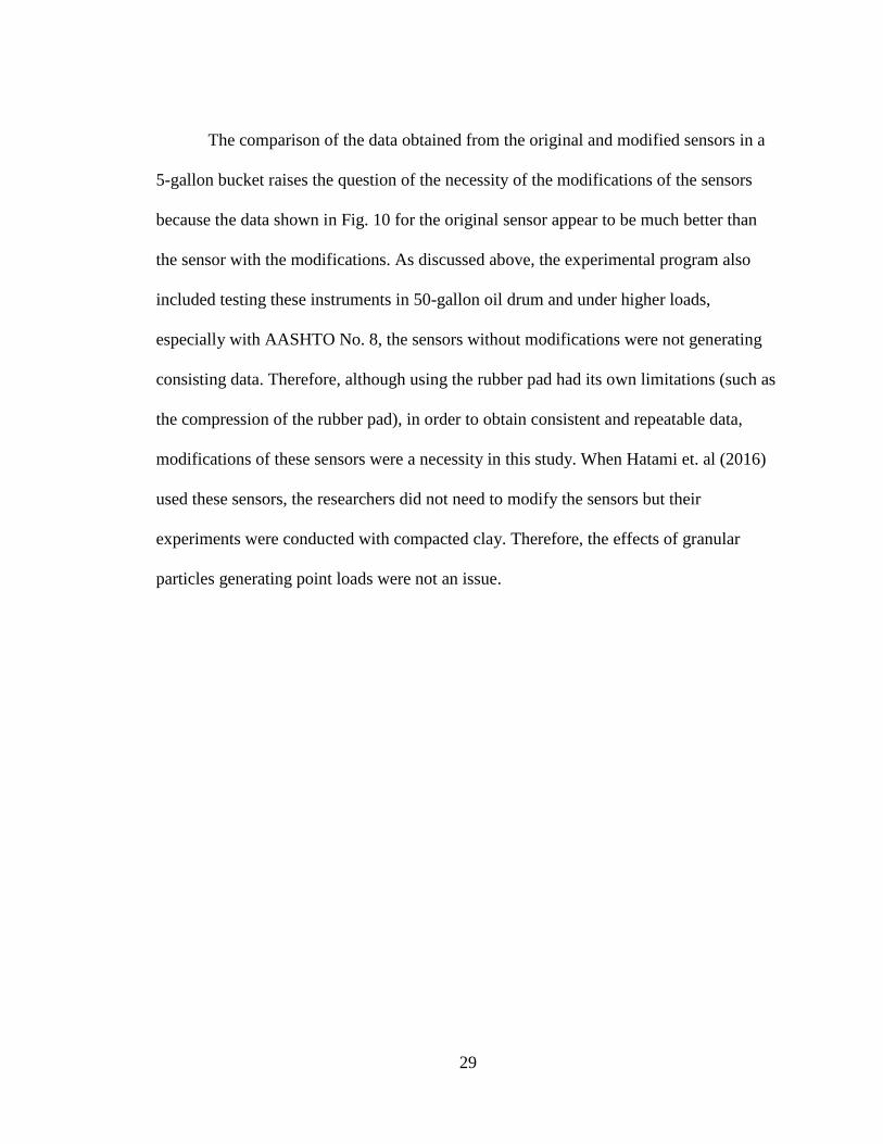
When the data shown in Fig. 10 is compared, it is not a surprise that the original

sensor (without any modifications) shows stress measurement in day one around 3.4 kPa,

which is very close to the applied theoretical stress. This is because this sensor was

calibrated with this soil hence matching results with the applied stress. However, it is

important to note that with time the stress readings did not change. At the same time, the

stress measured from the modified FSR showed a value of 16.1kPa, which was

significantly higher than the applied stress and is believed to be due to the rubber pad

added on to the sensor. The measured value for modified FSR however decreased over

time and stabilized around 6.1 kPa. There were two differences between the readings

28

from these two different sensors. One of these differences was due to the difference in

calibration methods and the other difference was due to the difference of modifications.

Therefore, using the stress measurement at day 45, a factor was defined to capture the (i)

effect of particular soil pressure on the modified sensor and (ii) effect of the compression

of the rubber pad on the modified sensor. This factor for the experiments with sand was

determined as 2.5 and with AASHTO No. 8 as 3.6 respectively. These factors were then

applied to all stress measurements obtained from all modified sensors used in the SSME

before the measurements were compared against the theoretical results and results

obtained from the RPC sensor. Therefore, all results shown in the subsequent sections

already include these applied factors to account for the differences in soil type and the

compression of the rubber pad.

Figure 10: Stress relaxation of rubber pad over time

29

The comparison of the data obtained from the original and modified sensors in a

5-gallon bucket raises the question of the necessity of the modifications of the sensors

because the data shown in Fig. 10 for the original sensor appear to be much better than

the sensor with the modifications. As discussed above, the experimental program also

included testing these instruments in 50-gallon oil drum and under higher loads,

especially with AASHTO No. 8, the sensors without modifications were not generating

consisting data. Therefore, although using the rubber pad had its own limitations (such as

the compression of the rubber pad), in order to obtain consistent and repeatable data,

modifications of these sensors were a necessity in this study. When Hatami et. al (2016)

used these sensors, the researchers did not need to modify the sensors but their

experiments were conducted with compacted clay. Therefore, the effects of granular

particles generating point loads were not an issue.

30

CHAPTER SIX: RESULT

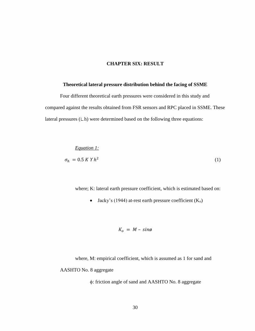
Theoretical lateral pressure distribution behind the facing of SSME

Four different theoretical earth pressures were considered in this study and

compared against the results obtained from FSR sensors and RPC placed in SSME. These

lateral pressures ( h) were determined based on the following three equations:

Equation 1:

𝜎ℎ = 0.5 𝐾 ϒ ℎ2 (1)

where; K: lateral earth pressure coefficient, which is estimated based on:

Jacky’s (1944) at-rest earth pressure coefficient (Ko)

𝐾𝑜 = 𝑀 – 𝑠𝑖𝑛ø

where, M: empirical coefficient, which is assumed as 1 for sand and

AASHTO No. 8 aggregate

: friction angle of sand and AASHTO No. 8 aggregate

31

Rankine’s (1857) active earth pressure coefficient (Ka)

𝐾𝑎 =( 1 − 𝑠𝑖𝑛 𝜙)

(1 + 𝑠𝑖𝑛 𝜙)

: unit weight of sand or AASHTO No. 8 aggregate used in this study, and

h: thickness of the sand or AASHTO No. 8 in the SSME

M: empirical coefficient, which is assumed as 1 for sand and AASHTO No. 8

aggregate

: friction angle of sand and AASHTO No. 8 aggregate

Equation 2:

𝜎ℎ = 0.72 𝐾𝑎 ϒ 𝑆𝑣2 (2)

where; Ka: Rankine’s active lateral earth pressure coefficient,

: unit weight of sand or AASHTO No. 8 aggregate used in this study, and

Sv: spacing between vertical reinforcement in the SSME.

Equation 3:

𝜎ℎ = 0.5 𝐾𝑎 ϒ 𝑆𝑣2 (3)

32

where; Ka: Rankine’s active lateral earth pressure coefficient,

: unit weight of sand or AASHTO No. 8 aggregate used in this study, and

Sv: spacing between vertical reinforcement in the SSME.

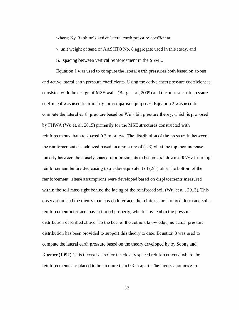
Equation 1 was used to compute the lateral earth pressures both based on at-rest

and active lateral earth pressure coefficients. Using the active earth pressure coefficient is

consisted with the design of MSE walls (Berg et. al, 2009) and the at–rest earth pressure

coefficient was used to primarily for comparison purposes. Equation 2 was used to

compute the lateral earth pressure based on Wu’s bin pressure theory, which is proposed

by FHWA (Wu et. al, 2015) primarily for the MSE structures constructed with

reinforcements that are spaced 0.3 m or less. The distribution of the pressure in between

the reinforcements is achieved based on a pressure of (1/3) σh at the top then increase

linearly between the closely spaced reinforcements to become σh down at 0.7Sv from top

reinforcement before decreasing to a value equivalent of (2/3) σh at the bottom of the

reinforcement. These assumptions were developed based on displacements measured

within the soil mass right behind the facing of the reinforced soil (Wu, et al., 2013). This

observation lead the theory that at each interface, the reinforcement may deform and soil-

reinforcement interface may not bond properly, which may lead to the pressure

distribution described above. To the best of the authors knowledge, no actual pressure

distribution has been provided to support this theory to date. Equation 3 was used to

compute the lateral earth pressure based on the theory developed by by Soong and

Koerner (1997). This theory is also for the closely spaced reinforcements, where the

reinforcements are placed to be no more than 0.3 m apart. The theory assumes zero

33

lateral pressure at the top of each reinforcement spacing due to frictional resistance and

then pressure linearly increases until the bottom of the reinforcement spacing as

computed with Equation 3.

Figure 11: Theoretical earth pressure distributions, bin pressure distribution and Soong and Koerner pressure

distribution based on 0.2m reinforcement spacing

Distribution of each of these pressures are provided in Fig. 11, which were

computed using the actual shear strength of the sand and AASHTO No. 8 aggregate used

in this study. It is to be noted that the results at the very top and bottom of the pit may not

be good enough for the comparison. The bottom of the pit has a stiff concrete floor,

therefore, creating a boundary effect in the bottom sensor measurement which will cause

faulty reading in the sensor. The top portion may not be compacted uniformly throughout

34

the pit and thus may not induce enough current difference to provide the pressure

measurement. Any measurement in between is assumed to be good for comparison with

theoretical pressure distribution.

Measured lateral pressure distribution from SSME with AASHTO No. 8 aggregate

The measured lateral pressures from unreinforced AASHTO No. 8 aggregate (no

geotextile) from FSR sensors are shown in Fig. 12a. The figure also depicts the

boundaries for each placement of aggregate for all three scenarios. For example, 0.2 m

layer boundary in Fig. 11a represents the experimental results obtained from the 0.2 m

thick layer and the pressure response at 0.2 m height from the bottom of the SSME. For a

0.4 m thick layer, 0.2 m showed in Fig. 12a would represent mid-depth from the bottom.

The results from all layer thicknesses show consistent lateral stress distribution,

validating the repeatability of the measurements from the FSR sensors.

(a)

35

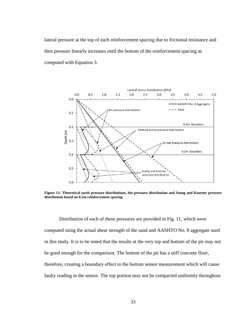
Figure 12: Lateral stress measurements from FSR sensors placed in SSME from AASHTO No. 8 aggregate that

is (a) unreinforced (no geotextile) (b) reinforced with 0.2 m spaced geotextile, and (c) reinforced with 0.1 m

spacing

The lateral pressure distributions recorded in SSME with 0.2 m reinforcement

spacing (with geotextile) with AASHTO No. 8 aggregate are shown in Fig. 12b. In this

(b)

(c)

36

figure, 0.2 and 0.4 m boundaries represent the location of the geotextiles. Both results

from 0.4 and 0.6 m thick layers demonstrate the stress rebound around the reinforcement

boundaries. When the measured pressure distribution from 0.2, 0.4, and 0.6 m

experiments are compared, the results show that in all layer thicknesses, the pressure

distribution increases with depth to a point and then decreases at the bottom of the SSME.

This behavior is most likely because of the very stiff boundary (i.e., concrete floor) at the

bottom of the SSME set-up. The results from all three-layer thicknesses show consistent

measurements.

The lateral pressure distributions recorded in SSME with 0.1m reinforcement

spacing (with geotextile) with AASHTO No. 8 aggregate are shown in Fig. 12c. In this

figure, 0.1 thru 0.5 m boundaries represent the location of the geotextiles. As seen in the

figure, the measurements obtained with the insertion of secondary reinforcement at 0.1 m

spacing has changed compare to the results seen in Fig. 12b although this effect is more

pronounced between the layers of 02 m thru 0.5 layers. The overall lateral stress increases

with depth and the overall magnitude compared to the distribution shown in Fig. 12b do

not seem to be significantly different. This could be due to the fact that SSME

measurements are obtained based on the self-weight of the material and were only 0.6 m

thick. Perhaps with thicker layers the difference in magnitude between the 0.1 and 0.2 m

spaced structures could be more pronounced.

Measured lateral pressure distribution from SSME with sand

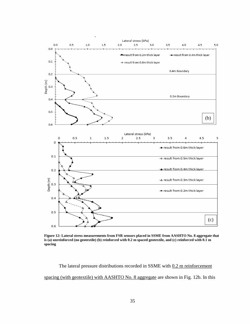
The lateral earth pressure distributions recorded from unreinforced SSME with

sand (no geotextile) from FSR sensors are shown in Fig. 13a for all three different layer

37

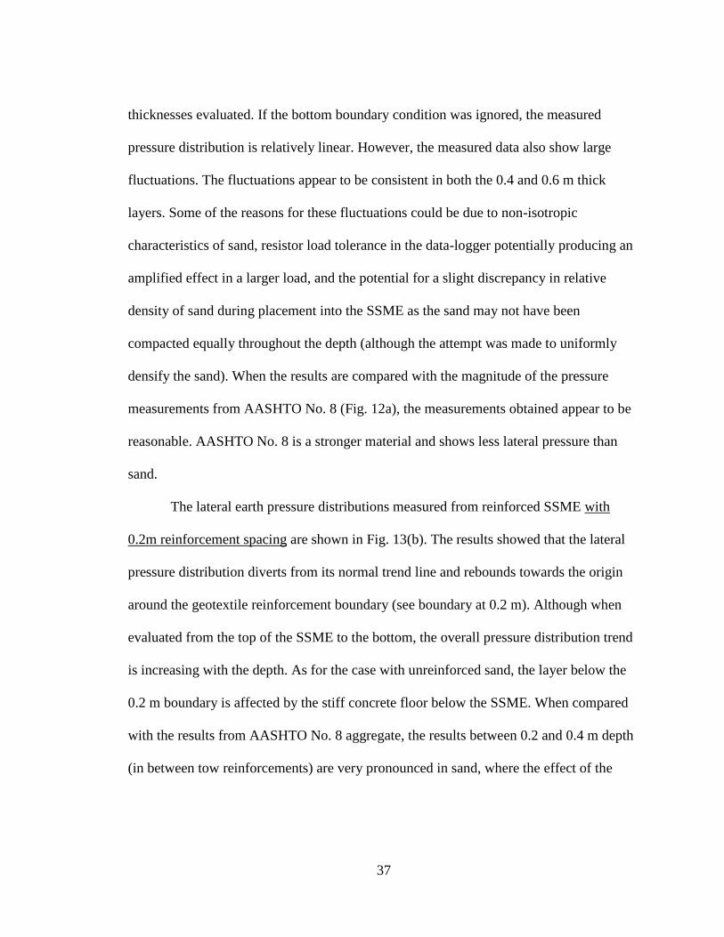
thicknesses evaluated. If the bottom boundary condition was ignored, the measured

pressure distribution is relatively linear. However, the measured data also show large

fluctuations. The fluctuations appear to be consistent in both the 0.4 and 0.6 m thick

layers. Some of the reasons for these fluctuations could be due to non-isotropic

characteristics of sand, resistor load tolerance in the data-logger potentially producing an

amplified effect in a larger load, and the potential for a slight discrepancy in relative

density of sand during placement into the SSME as the sand may not have been

compacted equally throughout the depth (although the attempt was made to uniformly

densify the sand). When the results are compared with the magnitude of the pressure

measurements from AASHTO No. 8 (Fig. 12a), the measurements obtained appear to be

reasonable. AASHTO No. 8 is a stronger material and shows less lateral pressure than

sand.

The lateral earth pressure distributions measured from reinforced SSME with

0.2m reinforcement spacing are shown in Fig. 13(b). The results showed that the lateral

pressure distribution diverts from its normal trend line and rebounds towards the origin

around the geotextile reinforcement boundary (see boundary at 0.2 m). Although when

evaluated from the top of the SSME to the bottom, the overall pressure distribution trend

is increasing with the depth. As for the case with unreinforced sand, the layer below the

0.2 m boundary is affected by the stiff concrete floor below the SSME. When compared

with the results from AASHTO No. 8 aggregate, the results between 0.2 and 0.4 m depth

(in between tow reinforcements) are very pronounced in sand, where the effect of the

38

geotextile reinforcement can be seen clearly. Whereas in the AASHTO No. 8 aggregate

measurements, the effect of the geotextile at 0.2 m depth is not as pronounced

(a)

(b)

39

Figure 13: Lateral stress measurements from FSR sensors placed in SSME from sand that is (a) unreinforced

(no geotextile) (b) reinforced with 0.2 m spaced geotextile, and (c) reinforced with 0.1 m spacing.

Fig. 13c shows the lateral stress distribution in sand with 0.1 m reinforcement

spacing. The horizontal lines drawn in this figure depict the 0.1m layer intervals. The

result shows no notable change in pressure distribution in sand when the reinforcement

spacing is decreased to half. With the lack of any connection to the facing, the secondary

reinforcement appears to remain passive and therefore no effect on the lateral pressure

was seen for any given layer thickness. The results obtained from different layer

thicknesses show consistent trends. When the results were evaluated particularly for the

pressure distribution obtained from the 0.6 m thick layer and in between 0.2 and 0.4 m

depths (where the geotextiles are frictionally connected to the facing), at the bottom of

the reinforcement (at 0.4 m depth) the trend appears to be similar to the trend shown in

Fig 13b (sand with reinforcements placed at 0.2 m spacing). However, similar

comparison is not observed at the top of the reinforcement (at 0.2 m depth). In that

(c)

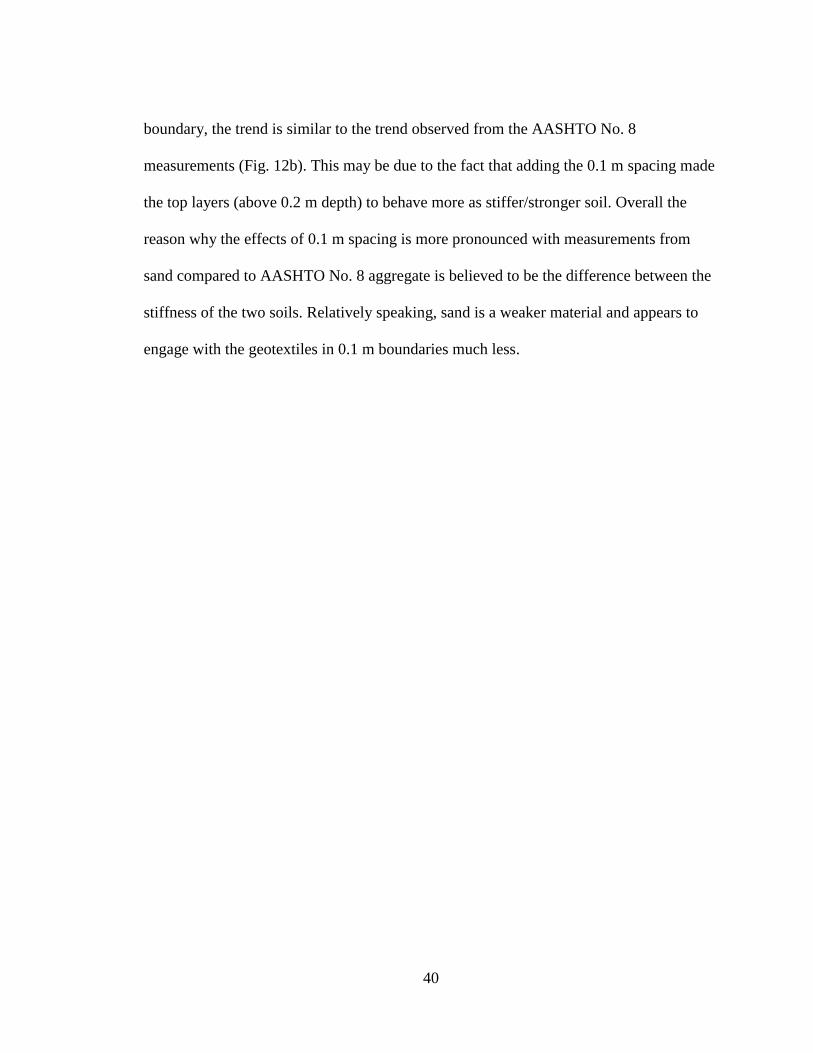
40

boundary, the trend is similar to the trend observed from the AASHTO No. 8

measurements (Fig. 12b). This may be due to the fact that adding the 0.1 m spacing made

the top layers (above 0.2 m depth) to behave more as stiffer/stronger soil. Overall the

reason why the effects of 0.1 m spacing is more pronounced with measurements from

sand compared to AASHTO No. 8 aggregate is believed to be the difference between the

stiffness of the two soils. Relatively speaking, sand is a weaker material and appears to

engage with the geotextiles in 0.1 m boundaries much less.

41

CHAPTER SEVEN: DISCUSSION

Comparison of SSME results from AASHTO No. 8 aggregate with theoretical

pressure distribution

The unreinforced measurements were compared against the lateral pressure

distributions computed with Equation 1 both with at-rest and Rankine’s pressure

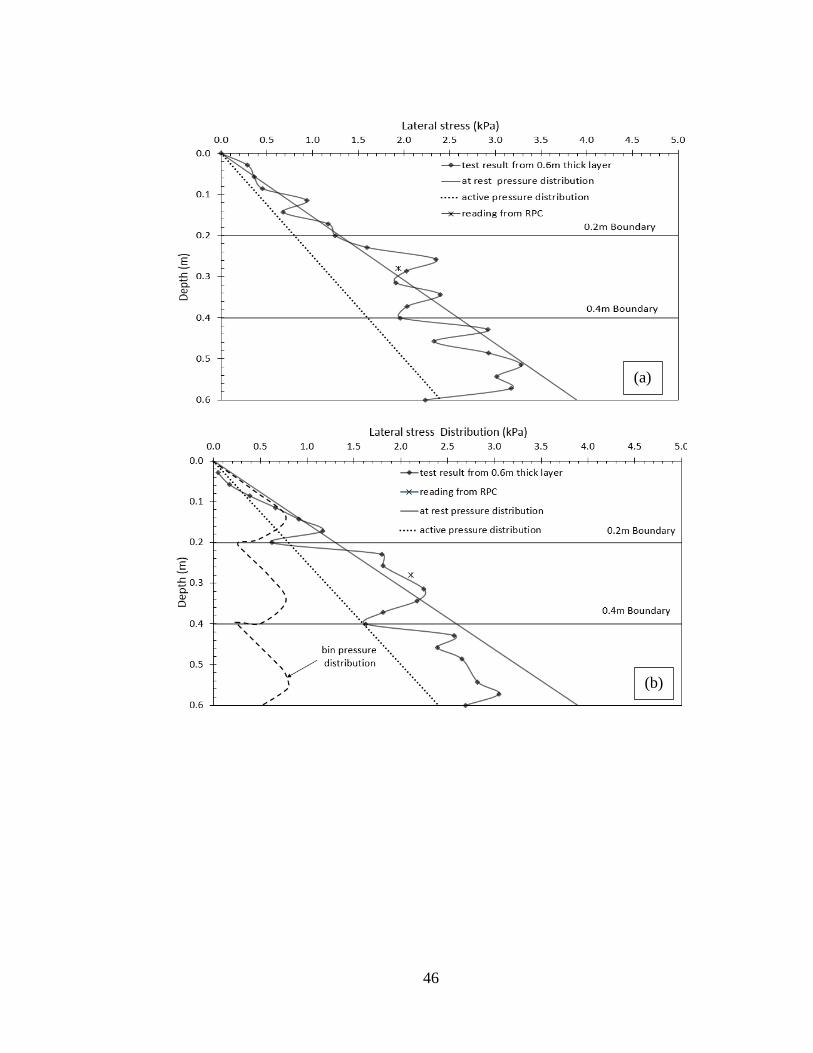
coefficients. Fig. 14a shows the comparison for the 0.6 m thick SSME measurements. If

the fluctuation of the measured value at the bottom due to stiff concrete is ignored, the

measured value is in very well agreement with the at rest pressure distribution. In this

figure, measurement from RPC sensor is also presented. The RPC measurement matches

well with both FSR measurement and also the theoretical at-rest pressure distribution. On

the topmost 0.5 m layer (i.e., 0.1 m depth), the pressure distribution follows the active

earth pressure trend line. This may be because the top layer at 0.6 m did not have a

reinforcement and the aggregate may not have been as compacted at the very top layer.

The effect of the reinforcement in the lateral earth pressure measurement can be

seen in Fig. 14b. These measurements were compared against the pressure distributions

computed with all of the equations (Equations 1 thru 3). When the measured FSR

readings are compared with the theoretical computations, it is seen that for the top 0.4 m

layer, the distribution follows at-rest trend line and then gets closer to active pressure.

The RPC measurement also matches the pressure from FSR and the theoretical at-rest

42

pressure. The figure also shows pressure distributions based on Equations 2 and 3. It is

interesting to see that, overall the trend (especially in between 0.2 and 0.4 m depths) is

close to the theoretical bin pressure distribution; however, the magnitude of the pressure

from bin pressure and what is measured are significantly different. The pressure

distribution Soong and Koerner’s theory also appear to be grossly smaller than what was

measured. Recalling the FHWA guideline, bin pressure and Soong and Koerner

distributions are independent of the height of the wall and depends on the reinforcement

spacing and the shear properties of the backfill material. Based on the measurements, the

pressure behind the facing of the wall does not appear to be independent of the height of

the wall and increases with the depth.

(a)

43

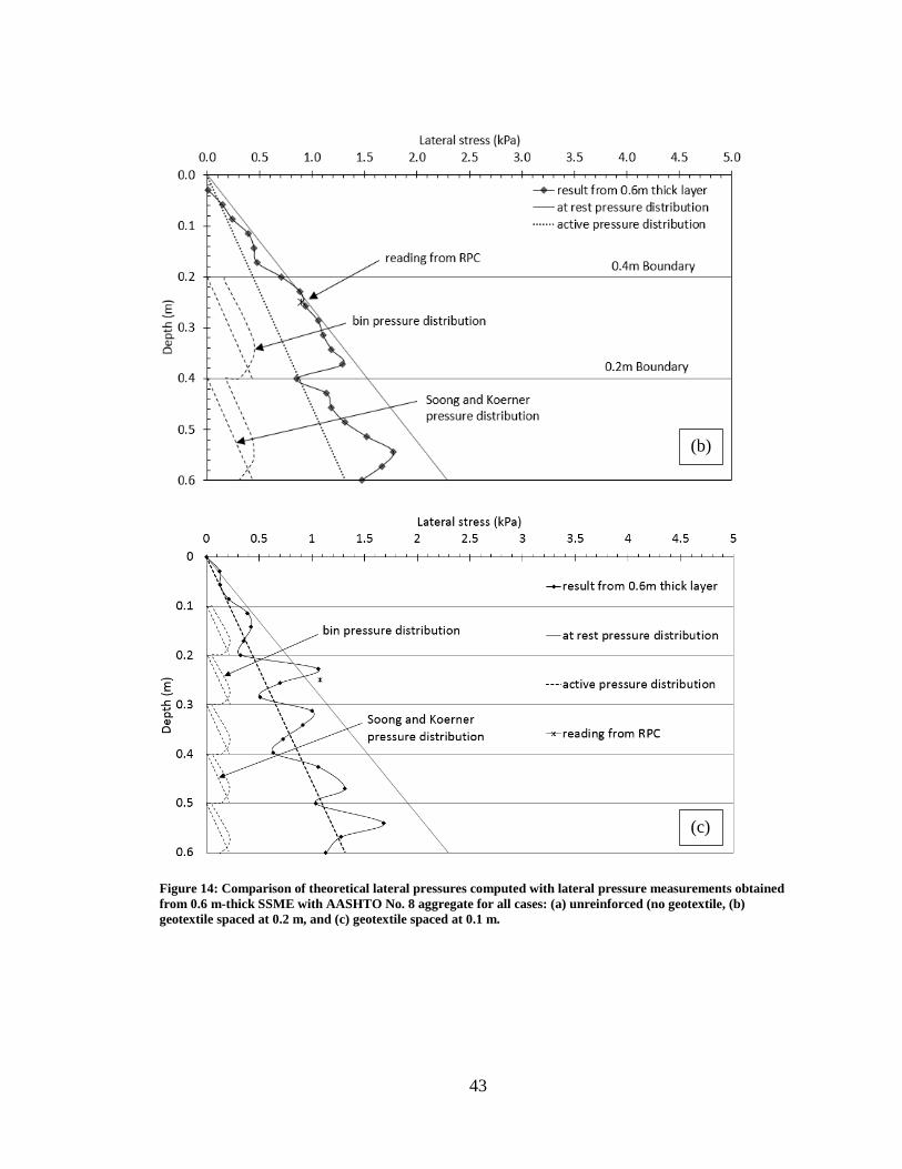
Figure 14: Comparison of theoretical lateral pressures computed with lateral pressure measurements obtained

from 0.6 m-thick SSME with AASHTO No. 8 aggregate for all cases: (a) unreinforced (no geotextile, (b)

geotextile spaced at 0.2 m, and (c) geotextile spaced at 0.1 m.

(b)

(c)

44

When the lateral pressure measurements from SSME reinforced with 0.1 m

spacing is compared, the measured pressure distribution appears to follow the active

lateral earth pressure trend than at-rest pressure distribution trend (Fig. 14c). This may

not be because of the movement of the wall causing the pressure condition to change (as

no signs of movement were observed during the experiments) but it may be that the

presence of the closely spaced reinforcement effectively restrained the lateral movement

of the aggregate. This would cause in an overall decrease in the lateral earth pressure

measurement as seen in the figure. Also, it is noteworthy that the RPC measurement and

the FSR measurement at the same depth are matching well as well. Both of the readings

are however offset from the at rest pressure at the same depth. The bin pressure

distribution and the distribution by Soong and Koerner are not matching numerically with

the measurement made by FSR but there are few things to note: (i) When the individual

pressure distribution in between two reinforcement zone is compared together, the

pressure distribution pattern matches very well with each other. Numerically, however,

they are very far from each other. (ii) There is a decrease in the overall pressure

distribution when the reinforcement spacing is decreased to half. This is potential because

of the restraining effect of the reinforcement on the aggregate lateral movement.

Comparison of SSME result with theoretical pressure distribution for sand

Fig. 15a shows the comparison of the FSR measurements within unreinforced

sand experiment and the lateral pressures computed with the theoretical pressure

distributions based on at-rest and active pressure conditions. Similar to the AASHTO No.

8 aggregate, the overall pressure distribution is in agreement with the theoretical at-rest

45

pressure distribution, except the pressure decreases at the bottom portion of the SSME.

As discussed earlier, this reduction is expected because of the stiff concrete floor at the

bottom of the SSME except for sand, this reduction can be seen much more pronounced

then with AASHTO No. 8 aggregate. Also, when measurements from FSR are compared

against the RPC measurement, both instruments show results that are in agreement with

the theoretical at-rest pressure distribution.

When the lateral earth pressures from the sand experiments with 0.2 m spaced

geotextile reinforcements are compared with theoretical stress distributions (Fig. 15b),

the values at the top and bottom of the reinforcements show measurements close to the

active earth pressure distribution but in between the reinforcements, the values increase

to close to at-rest condition. The shape of the pressure distribution resembles the

distribution from the bin pressure theory except the magnitudes are much higher and

unlike the bin pressure distribution, the pressures continue to increase with depth. The

measurement from the RPC is in agreement with the FSR measurements. At the bottom

of the SSME, layer between the 0.4m boundary and concrete floor, the pressure drops

from at rest pressure to the active pressure.

46

(a)

(b)

47

Figure 15: Comparison of theoretical lateral pressures computed with lateral pressure measurements obtained

from 0.6 m-thick SSME with sand aggregate for all cases: (a) unreinforced (no geotextile, (b) geotextile spaced at

0.2 m, and (c) geotextile spaced at 0.1 m.

Fig. 14c depicts the comparison for the case where the geotextile reinforcements

were spaced at 0.1 m increments. The effects of the 0.1 m reinforcements have been

discussed in the previous section, however in this comparison, especially between the 0.2

and 0.4 m spacing, the shape of the pressure distribution is similar to the shape of the

distribution from 0.2 m spaced geotextile case. However, with 0.1 spacing, the magnitude

of the lateral pressures at 0.2 and 0.4 m boundaries do not reduce as much as in the case

where geotextiles were spaced at 0.2 m in the SSME. In general, bin pressure distribution

and distribution by Soong and Koerner do not capture the observed behavior. In the 0.1 m

spacing condition, even the shape of the stress distribution resembles the bin pressure

theory. The result obtained from RPC is in agreement with the measurements from FSR.

(c)

48

CHAPTER EIGHT: PRACTICAL IMPLICATIONS, CONCLUSIONS, AND

LIMITATIONS

The results obtained from this study show that the FSR sensor has a potential to

measure lateral stress distribution behind the facing of the earth retaining structures

especially when the reinforcements are placed closed to each other (such as less than 0.3

m apart). The results show that the rectangular earth pressure (RPC) sensor used in this

study also produces results that are similar to the FSR measurements and within the

bounds of theoretical stress distributions. This information validates the results obtained

from FSR sensors. Therefore, the major contribution of this research is that it presents a

new instrument that may be used to measure in relevant geotechnical projects. However,

it should be noted that proper calibration and protection of the instrument is necessary to

obtain reliable results. There are certainly other instruments available in the market,

however; the size and the cost of these sensors provide an alternative especially if the

interest is to measure a continuous distribution with depth.

To the best of the authors’ knowledge, this is the first study where lateral stress

distribution behind the closely spaced geotextile reinforcements have been measured

continuously with depth. This allowed the measurements to be compared with the

theoretical stress distributions that are particularly developed to capture the stress

distribution between closely spaced geosynthetic reinforcements. The comparison

between the theoretical stress distributions and measured values show that closely spaced

49

reinforcements provide benefit in reducing pressures at the interface of soil and

geotextiles, however unlike what has been proposed before, the pressure distribution is a

function of depth (not constant throughout the structure). Also, the results show that the

magnitude of the lateral stress behind the facing blocks are order of magnitude higher

than what is computed from the bin pressure and Soong and Koerner distributions

(although in all cases, the maximum stress measured in this study was less than 4 kPa).

Overall SSME was conducted based on 0.6 m thick layers (due to the limitations of the

laboratory study) and the measurements were obtained based on self-weight of the soils

used, however, with much higher structures and surcharge loads, the difference between

the theoretical and measured lateral stress magnitudes may become more important

especially in the case of designing the facing of the MSE structures constructed with

individual masonry blocks. . It may also be true that with additional depth, perhaps the

stresses at the facing will continue to reduce and at some point, become constant with

depth. However, this could not be verified in the laboratory due to the limitations of the

SSME set-up. Therefore, without a doubt that the concepts developed in this study need

to be tested at a reinforced wall with higher depths. It is understood that the design of the

facing blocks is also dependent on the interface friction between the geotextile

reinforcements and the concrete masonry blocks but this study provides an insight about

the lateral stress distribution that has not been captured before elsewhere. The soils tested

in this study were cohensionless in nature. In the case of soils with high fines content and

with cohesive nature, the stress distributions may appear to be different than what is

50

observed in this study. Although the FSR may also be used to test stress distributions in

such conditions.

The authors made an attempt to install FSR sensors to the back of facing blocks of

an actual MSE structure in the field, however, that attempt was made before the start of

this study. Therefore, at that time the inside knowledge of the instrument was limited.

The learning lessons from that experience showed that the FSR used in this research is

not water resistant and additional modification is required to protect it from water and

moisture. Also, at that time, the authors were not aware of the need to modify the sensor

with a rubber pad and a thin metal sheet and over time the sensors stopped producing

results. Although that was a failed attempt, the authors are confident that based on the

information gained from this study, these sensors may be used in the field, however

proper protection, modification, and calibration are required for each sensor. The authors

will attempt to use this sensor in the field as soon as the next project becomes available

for demonstration and will continue the SSME with soils that contain fines content

(particles finer than U.S. 200 sieve). In this study, the measurements were obtained in

between geotextile reinforcements, however future studies will include evaluation

between geogrids and metallic reinforcements.

51

APPENDIX A: CHARACTERIZATION OF SOIL

52

AASHTO No. 8:

Optimum unit weight

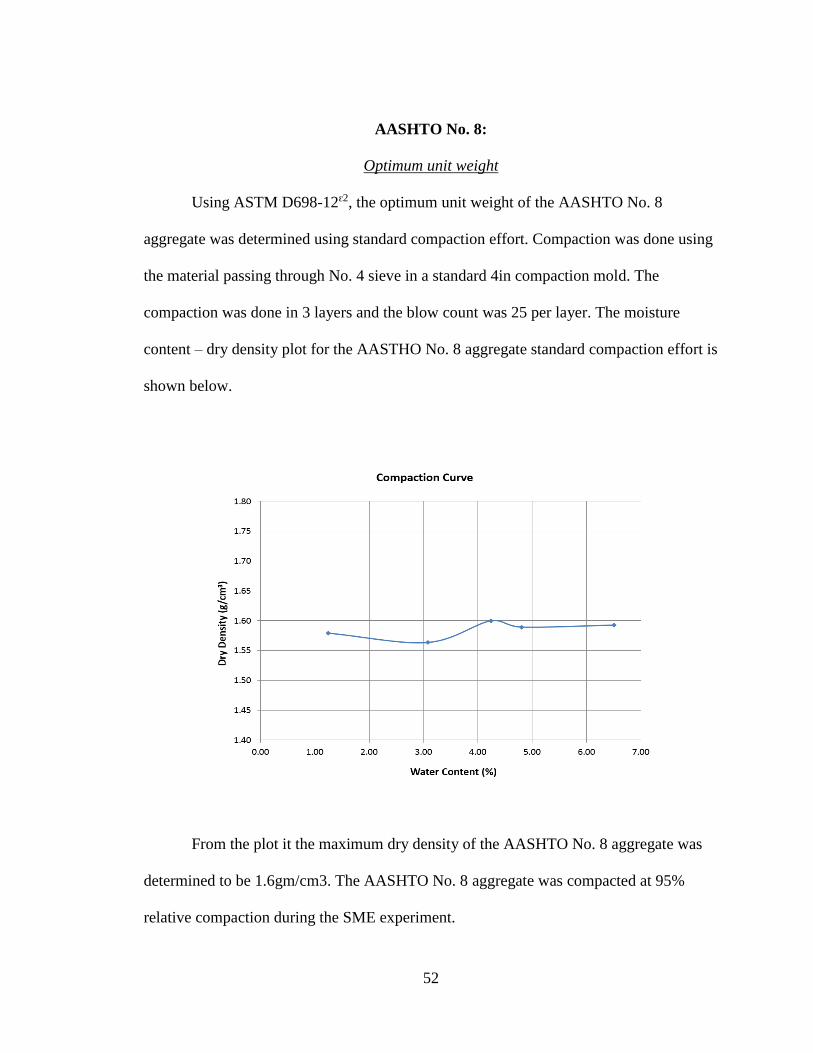
Using ASTM D698-12ԑ2, the optimum unit weight of the AASHTO No. 8

aggregate was determined using standard compaction effort. Compaction was done using

the material passing through No. 4 sieve in a standard 4in compaction mold. The

compaction was done in 3 layers and the blow count was 25 per layer. The moisture

content – dry density plot for the AASTHO No. 8 aggregate standard compaction effort is

shown below.

From the plot it the maximum dry density of the AASHTO No. 8 aggregate was

determined to be 1.6gm/cm3. The AASHTO No. 8 aggregate was compacted at 95%

relative compaction during the SME experiment.

53

Consolidated drained (CD) triaxial test by ASTM D7181

Consolidated drained triaxial test was performed on AASHTO No. 8 aggregate

using ASTM D7181. The Mohr’s circle diagram obtained from the triaxial test results are

shown below. From the experiment, the internal frictional angle was determined to be

47.6⁰.

Sand

Minimum Index Density Test and Unit weight of sand. (ASTM D4245-14)

The minimum Index density test of sand was carried out in the lab according to

ASTM standard. With all the necessary check that the ASTM specifies, it was determined

that the apparatus was fit for the test. The dropping of sand in the apparatus was slow and

54

steady and the drop height was maintained less than 1cm. The dropping of sand was done

in a spiral direction which is commonly called elephant trunk method. The test was

repeated 3 times for the best result and the minimum weight recorded in those 3 tests

were chosen for the minimum Index density test.

The photographs below are the scanned copy of the calculation performed to

determine that the apparatus used to determine Index density test was according to

ASTM standard and calculation of the Index density of the sand.

55

56

Maximum Index Density of soil and Unit weight of sand. (ASTM D4253-14)

The maximum index density test of sand was carried out in the lab according to

ASTM standard. The process used for the test was under ASTM standard. However, there

was some discrepancy in the equipment used. Due to lack of proper vibrator machine, the

sieve vibrator was used for vibration of sand. The minimum surcharge load as specified

by ASTM was minimum 11Kg weight. About 14Kg of surcharge was applied to the sand

for densifying the sand. Care was taken so the surcharge load was evenly distributed on

the sand surface. The test was repeated 2 times and maximum density from the two was

chosen as maximum index density.

Photographs below show the test procedure and the calculation process to

determine the maximum index density.

57

58

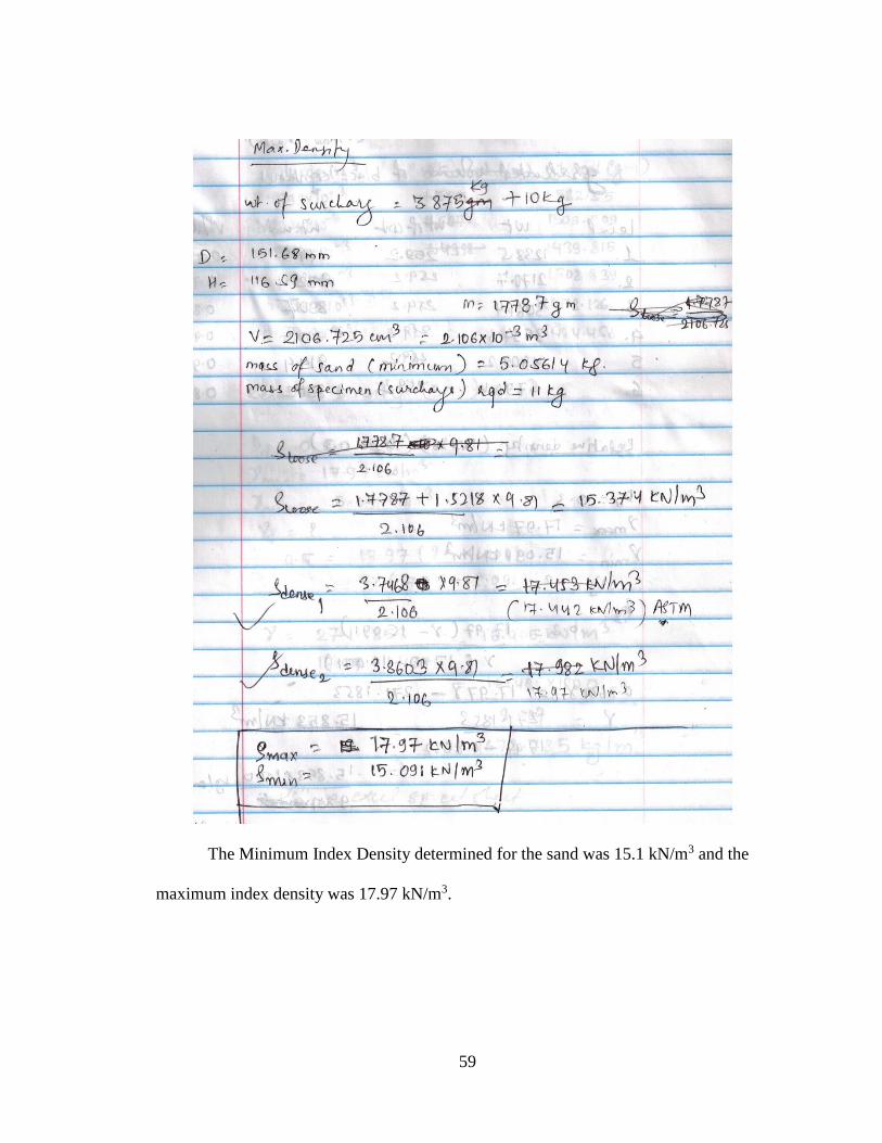
59

The Minimum Index Density determined for the sand was 15.1 kN/m3 and the

maximum index density was 17.97 kN/m3.

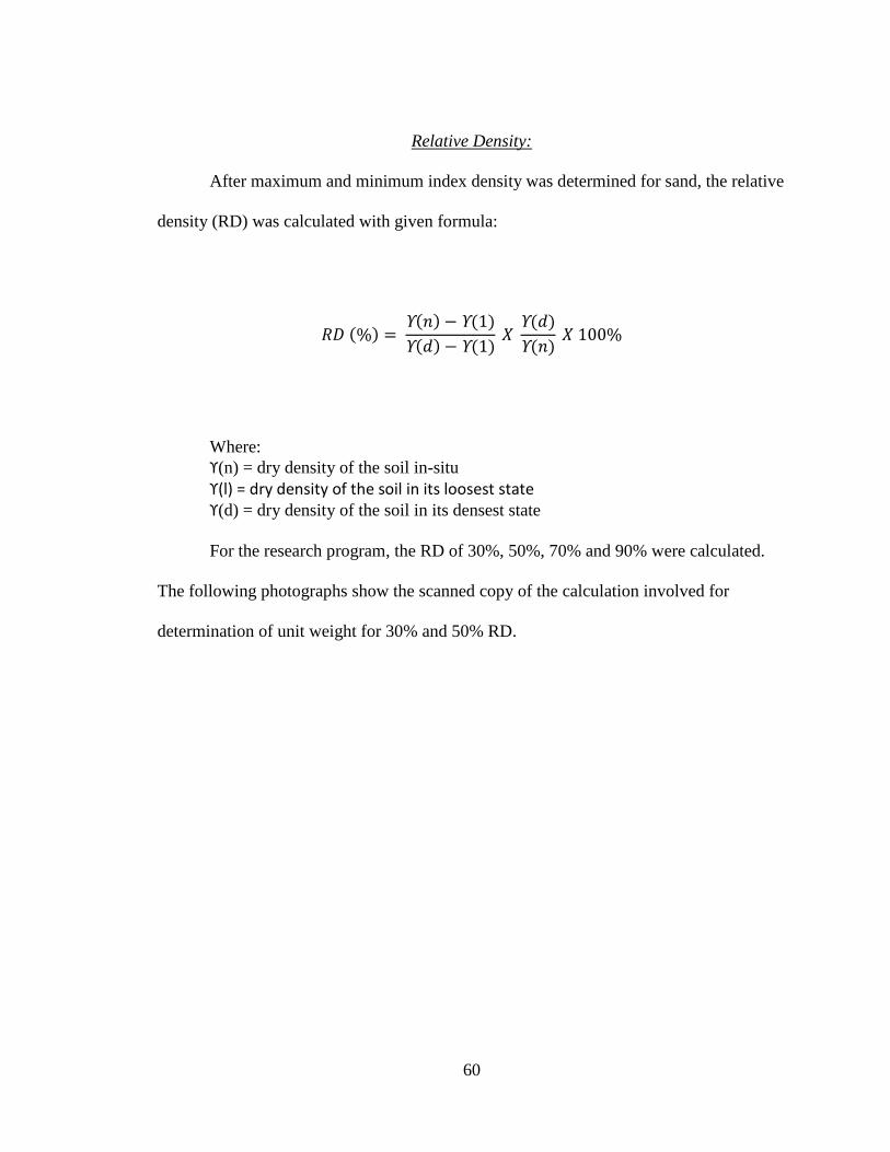
60

Relative Density:

After maximum and minimum index density was determined for sand, the relative

density (RD) was calculated with given formula:

𝑅𝐷 (%) = ϒ(𝑛) − ϒ(1)

ϒ(𝑑) − ϒ(1) 𝑋

ϒ(𝑑)

ϒ(𝑛) 𝑋 100%

Where:

ϒ(n) = dry density of the soil in-situ

ϒ(l) = dry density of the soil in its loosest state ϒ(d) = dry density of the soil in its densest state

For the research program, the RD of 30%, 50%, 70% and 90% were calculated.

The following photographs show the scanned copy of the calculation involved for

determination of unit weight for 30% and 50% RD.

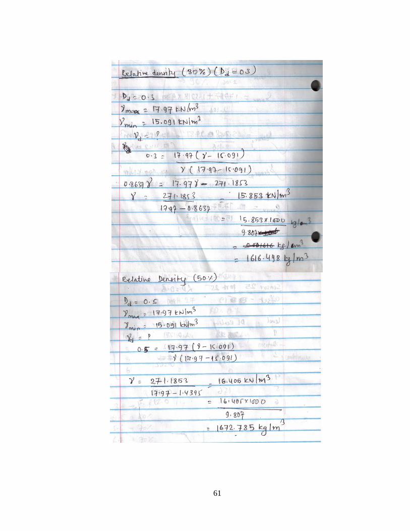
61

62

Consolidated drained (CD) triaxial test by ASTM D7181

Consolidated drained triaxial test was performed on sand using ASTM D7181.

The Mohr’s circle diagram obtained from the triaxial test results based on failure at peak

stress are shown below. From the experiment, the internal frictional angle was

determined to be 38.2⁰.

63

APPENDIX B: CALIBRATION OF FORCE SENSING RESISTOR (FSR)

64

Calibration of FSR as is

The experiment was initiated by calibration of the sensors by compacting play

sand at a different relative compaction of 30%, 50%, 70% and 90% in a black container

with 0.15m diameter and 0.3m height. The placement and compaction of the sand were

done in 0.05m thick layer. The best fit linear regression line was used to interpolate the

DAQ output. It was seen that as the overburden pressure over the sensor increased, the

stresses were distributed more toward the boundary and very less stress increment was

observed by the sensor. The calibration was then performed using 5-gallon homer bucket

by placing play sand in the homer bucket and compacted at different relative density.

Compaction of the sand was done by the tamping method. Photographs shown below are

at shown during various stages of calibration.

65

The calibration of the sensor was initiated with few sensors with same sensitivity

level based on the same level of sensor conductivity output level for same given input.

The calibration results from the bucket test from 30% RD compaction is shown below:

Shown below is the calibration result from 50% RD compaction:

66

Shown below is the calibration result from 70% RD:

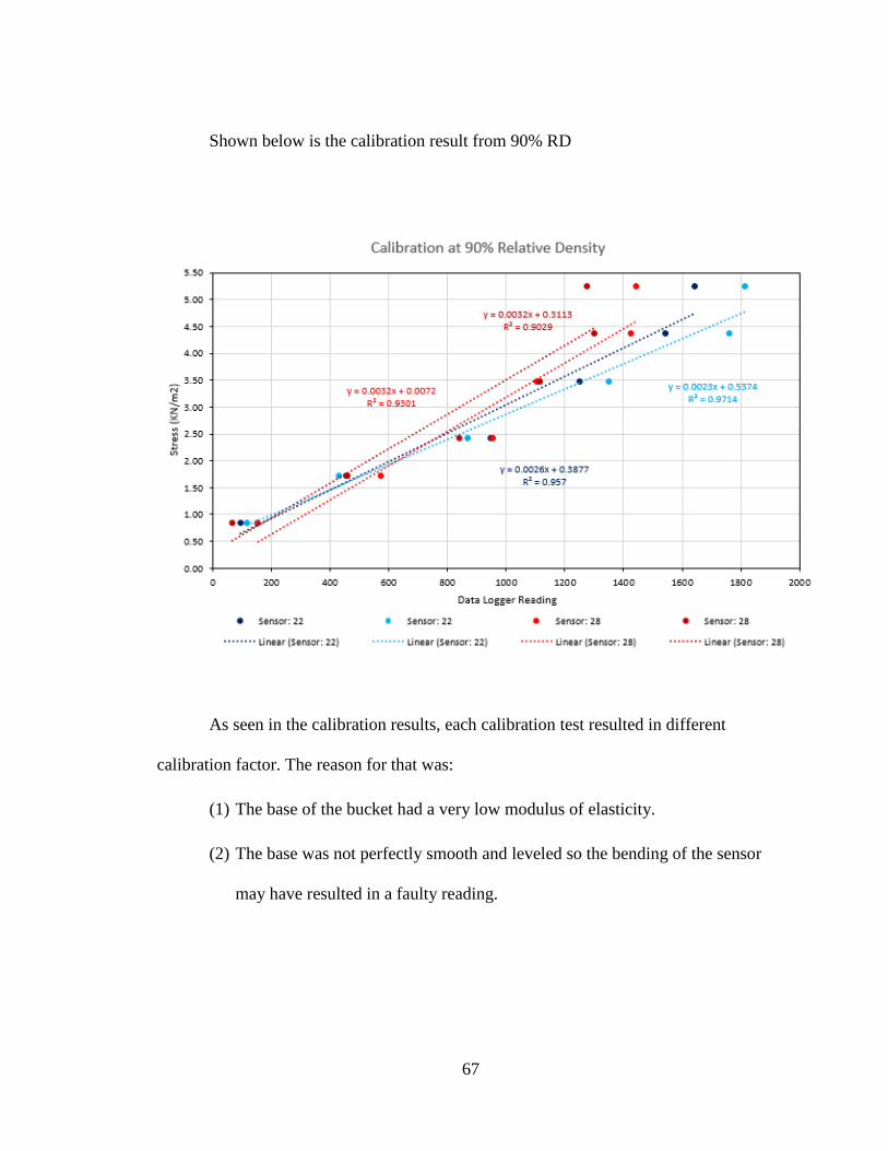
67

Shown below is the calibration result from 90% RD

As seen in the calibration results, each calibration test resulted in different

calibration factor. The reason for that was:

(1) The base of the bucket had a very low modulus of elasticity.

(2) The base was not perfectly smooth and leveled so the bending of the sensor

may have resulted in a faulty reading.

68

(3) At some point, it was seen that the stress from the sensor is more distributed

towards the boundary of the bucket than towards the base, the additional load

on the top had no effect on the conductivity of the sensor.

A new method was devised to eliminate the problem associated with the previous

method. A concrete base with a thin metal plate on top of it was introduced at the base of

the bucket as shown in the figure below. The method was named as Sensor/Metal-

Concrete (S/M-C) Calibration.

Furthermore, the height of the compaction was limited to 20 cm to ensure the

boundary issue had been eliminated. The result from the calibration at different RD is

presented below:

69

Shown below is the calibration result from 30% RD

Below is the calibration result from 50% RD

70

Below is the calibration result from 70% RD

71

Below is the calibration result from 90% RD

An experiment was performed on 55 gallons (208.2 liters) to confirm that the

calibration results from the bucket holds true in large setup and to check that the bucket

had no boundary issues. The experiments were performed at 70% RD. The results from

the drum test are shown below.

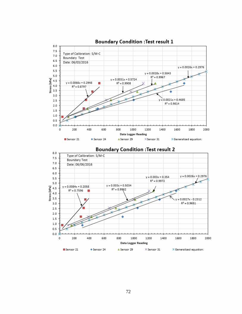
72

73

Calibration of Modified FSR

The calibration on modified FSR was done by placing dead weight on top of the

sensor and recording the output results in milliampere (mA). Result from modified FSR

calibration setup for all 32 sensors are shown below:

74

75

76

77

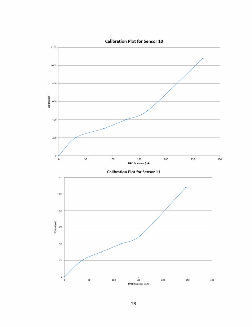
78

79

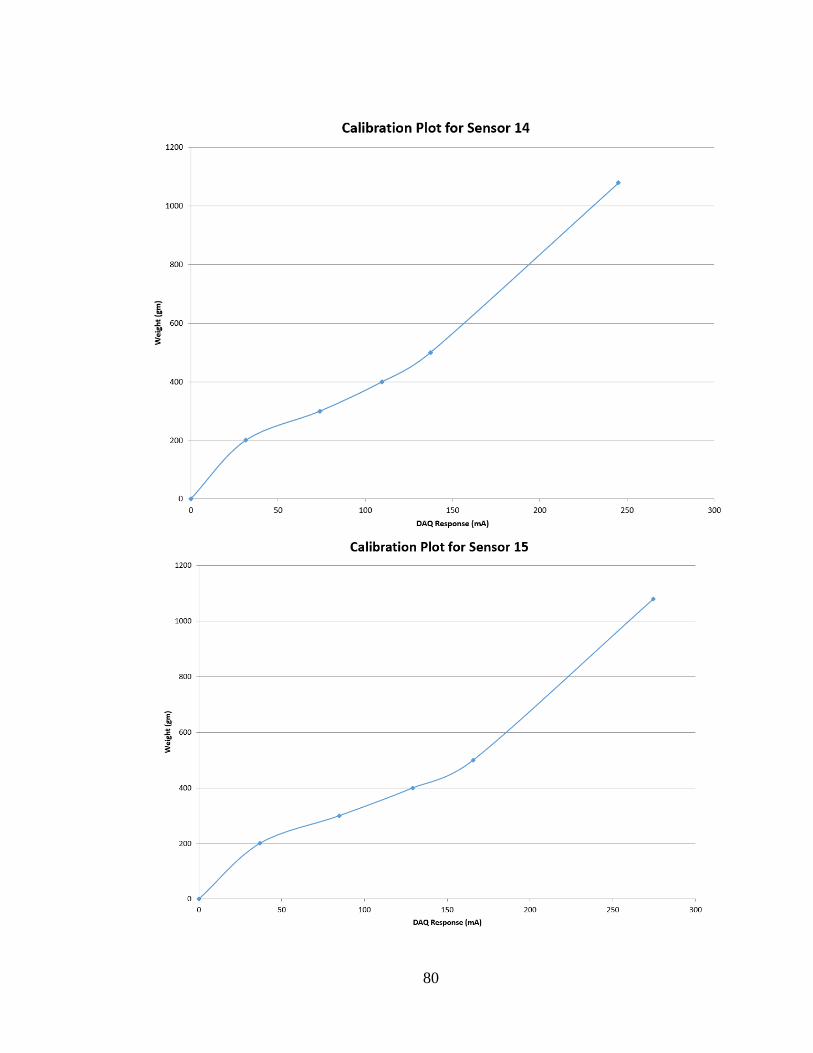
80

81

82

83

84

85

86

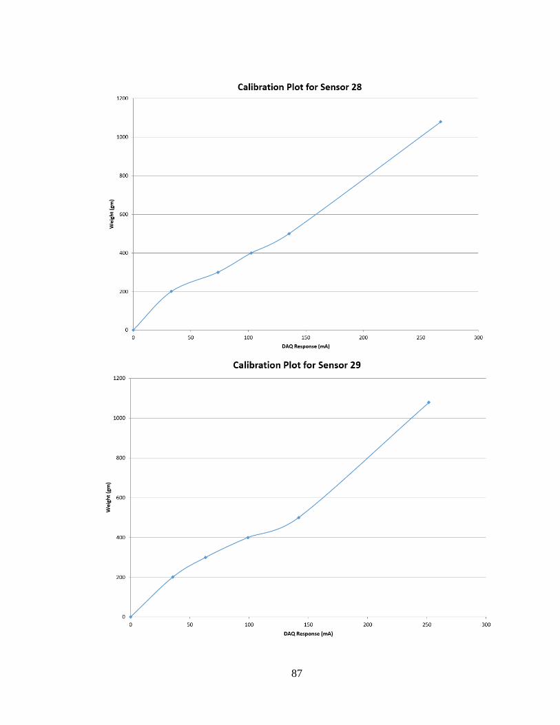
87

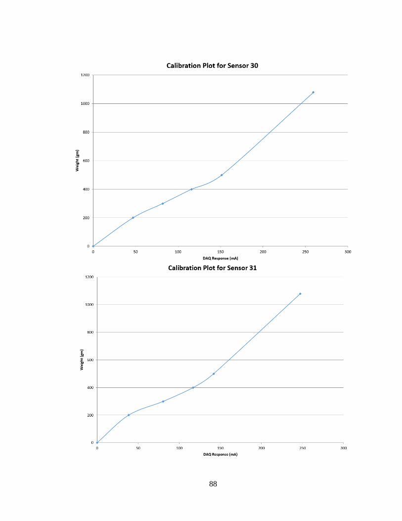
88

89

90

APPENDIX C: VERTICAL PRESSURE MEASUREMENTS FROM MODIFIED

FSR

91

Vertical Pressure Measurement

11 out of 32 sensors were installed in the base of the experimental pit to measure vertical

pressure from sand and AASHTO No. 8. The sensors were spread from the wall to the

center with the sensors placed equidistance from each other. More sensors were clustered

towards the center to observe the vertical stress change due to the placement of soil

without having boundary issue due to the presence of facing the wall. The arrangement of

the horizontally placed FSR to measure vertical pressure is shown below on the left:

The figure on the right represents the FSR being covered with sand to protect the

punching of AASHTO No. 8 aggregate into the sensor. The results from vertical pressure

variation at a different location away from the facing wall in unreinforced AASHTO No.

8 SME is shown below. In the figure, the stress variation is shown against the distance

from the facing. The line with a dot in the figure represents measured pressure line from

FSR whereas the straight line without dot represents theoretical pressure.

92

The vertical pressure variation with respect to the facing of the wall in reinforced

(0.2m) AASHTO No. 8 SME is shown below:

93

The vertical pressure variation with respect to the facing of the wall in reinforced

(0.1m) AASHTO No. 8 SME is shown below. The result obtained from the experiment is

presented in six layers as shown below:

The results from vertical pressure variation at a different location away from the

facing wall in unreinforced sand SME is shown below.

94

The results from vertical pressure variation at a different location away from the

facing wall in the reinforced sand (0.2m) SME is shown below.

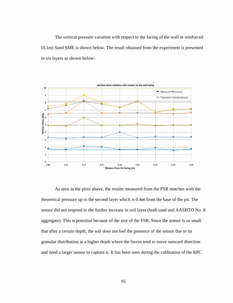
95

The vertical pressure variation with respect to the facing of the wall in reinforced

(0.1m) Sand SME is shown below. The result obtained from the experiment is presented

in six layers as shown below:

As seen in the plots above, the results measured from the FSR matches with the

theoretical pressure up to the second layer which is 0.4m from the base of the pit. The

sensor did not respond to the further increase in soil layer (both sand and AASHTO No. 8

aggregate). This is potential because of the size of the FSR. Since the sensor is so small

that after a certain depth, the soil does not feel the presence of the sensor due to its

granular distribution at a higher depth where the forces tend to move outward direction

and need a larger sensor to capture it. It has been seen during the calibration of the RPC

96

that the RPC captures the force due to the larger sensing area. No such issue as seen in

RPC reading from vertical stress measurement was seen during the calibration.

97

APPENDIX D: HYSTERESIS IN FSR

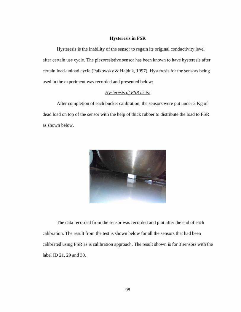
98

Hysteresis in FSR

Hysteresis is the inability of the sensor to regain its original conductivity level

after certain use cycle. The piezoresistive sensor has been known to have hysteresis after

certain load-unload cycle (Paikowsky & Hajduk, 1997). Hysteresis for the sensors being

used in the experiment was recorded and presented below:

Hysteresis of FSR as is:

After completion of each bucket calibration, the sensors were put under 2 Kg of

dead load on top of the sensor with the help of thick rubber to distribute the load to FSR

as shown below.

The data recorded from the sensor was recorded and plot after the end of each

calibration. The result from the test is shown below for all the sensors that had been

calibrated using FSR as is calibration approach. The result shown is for 3 sensors with the

label ID 21, 29 and 30.

99

It is seen that the sensitivity level of the sensor drops after certain load-unload

cycle (8th cycle on average in our case). It is to be noted that the maximum vertical stress

applied to the sensors in the bucket calibration was 3.5kPa.

Hysteresis of modified FSR:

The sensitivity of the modified FSR was recorded after completion of each SME.

The figure below shows the setup of the hysteresis test. The output result of modified

FSR after loading it with known load is recorded and presented below:

100

The output result of modified FSR placed at the bottom of the pit after loading it

with known load is recorded and presented below:

The data shown above are recorded from 11 sensors in the bottom of the pit which

measures vertical stresses. These sensors also experience highest amount of stresses than

that placed on the facing wall to measure lateral stresses. The maximum stress

experienced by these stress was 9.86 kPa from the sand test. It is seen that some of the

sensors have undergone through sensitivity level regardless of the modification.

4.004.404.805.205.606.006.406.807.207.608.008.40

0 2 4 6 8 10 12

stre

ss (

kPa)

No. of tests

Hysterisis chart

27

26

25

24

23

22

4.004.404.805.205.606.006.406.807.207.608.008.40

0 2 4 6 8 10 12

Stre

ss (

kPa)

No. of tests

Hysterisis chart

32

31

30

29

28

101

The hysteresis recorded from two sensor setup are hard to compare. The amount

of load placed on the sensor and loading method are not equal in both of the tests. Also,

the stress experienced in both experimental scenarios were not equal. The bucket

calibration had 3.5 kPa vertical stress whereas the SME had 9.8kPa vertical stress which

is roughly 3 times more than bucket calibration. A mechanism to compare the hysteresis

from two setups where the loading mechanism and amount of load applied should be

developed to compare this two setup.

102

APPENDIX E: BACKGROUND ON DESIGN

103

FHWA Manual Guidelines on Lateral earth pressure

In 1993, Chou and Wu investigated and predicted the performance of GRS wall

using the finite element method DASCAR. The reinforcement spacing behind the wall

was kept 0.3m. The lateral earth pressure against the wall face, against the back of

reinforced soil mass, and stress of plane of maximum tensile force in the reinforcement

were analyzed and presented in the figure below:

(after Chou and Wu, 1993)

In 2011, FHWA report stated that the lateral earth pressure remains constant

throughout the depth of the facing of the GRS wall as shown in the figure below. The

closely spaced reinforced system effectively restrains the soil against the lateral

movement also restraining the lateral earth pressure. FHWA design manual considers

104

constant lateral earth pressure to evaluate its lateral earth pressure behind the facing of

the wall.

(After FHWA GRS-IBS Manual synthesis, 2011)

After Wu’s bin pressure theory, 2001)

The FHWA manual on GRS-IBS published in 2015 identified two different methods to

evaluate the lateral earth pressure on GRS wall facing. One of the methods to measure

lateral earth pressure was given by Wu in 2001. According to the theory, the pressure

diagram is near zero around the top reinforcement boundary and increases with depth

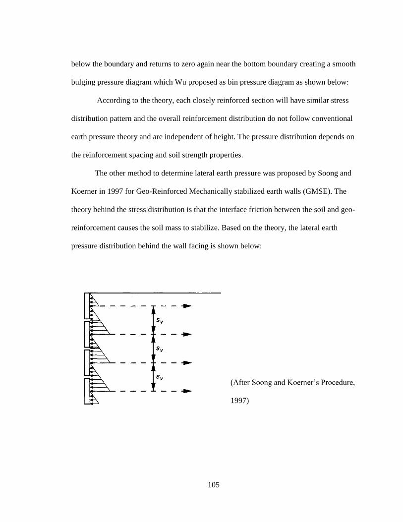
105

below the boundary and returns to zero again near the bottom boundary creating a smooth

bulging pressure diagram which Wu proposed as bin pressure diagram as shown below:

According to the theory, each closely reinforced section will have similar stress

distribution pattern and the overall reinforcement distribution do not follow conventional

earth pressure theory and are independent of height. The pressure distribution depends on

the reinforcement spacing and soil strength properties.

The other method to determine lateral earth pressure was proposed by Soong and

Koerner in 1997 for Geo-Reinforced Mechanically stabilized earth walls (GMSE). The

theory behind the stress distribution is that the interface friction between the soil and geo-

reinforcement causes the soil mass to stabilize. Based on the theory, the lateral earth

pressure distribution behind the wall facing is shown below:

(After Soong and Koerner’s Procedure,

1997)

106

The calculated lateral earth pressures from both approaches provide pressure

which is smaller than the Rankine active earth pressure. This is also supported by the

construction evidence of GMSE wall at Grand County, Colorado where the exerted

lateral pressure of a 16.8m (55 ft) high wall is less than the pressure at the active

condition.

107

REFERENCES

AASHTO. 2005. Standard specification for sizes of aggregate for road and bridge

construction. Washington, DC: AASHTO M43.

Abu-Hejleh, Naser M., Jorge G. Zornberg, Victor Elias, and Jim Watcharamonthein.

2003. "Desing Assesment of the Founders/Meadows GRS Abutment Structure."

Washington, D.C.: Transportation Researh Board.

Adams, Michael, Jennifer Nicks, Tom Stabile, Jonathan Wu, Warren Schlatter, and

Joseph Hartmann. 2011. Geosynthetic Reinforced Soil Integrated Bridge System,

Synthesis Report. Federal Highway Administration.

Adams, Mihael, Jennifer Nicks, Tom Stabile , Jonathan Wu, Warren Schlatter, and

Joseph Hartmann. 2012. Geosynthetic Reinforced Soil Integrated Bridge System

Interim Implementation guide. Federal Highway Administration.

Allen, T. M., B. R. Christopher, and R. D. Holtz. 1992. Performance of a 41-Foot High

Geotextile Wall. Final Report, Washington State Department of Transportation.

Allen, Tony M., and Richard J. Bathurst. 2001. Prediction of Soil Reinforcement Loads in

Mechanically Stabilized Earth Walls. Research Report, Washington State

Department of Transportation.

ASTM. 2014. "D4253-14 Standard Test Methods for Maximum Index Density and Unit

Weight of Soils Using a Vibratory Table." ASTM International.

doi:https://doi.org/10.1520/D4253-14.

ASTM. 2014. "D4254-14 Standard Test Methods for Minimum Index Density and Unit

Weight of Soils and Calculation of Relative Density." ASTM International.

doi:https://doi.org/10.1520/D4254-14.

ASTM. 2015. "D698-12 Standard Test Methods for Laboratory Compaction

Characteristics of Soil Using Standard Effort." ASTM International.

ASTM. 2011. "D7181-11 Standard Test Method for Consolidated Drained Triaxial

Compression Test for Soils." ASTM International.

Berg, R. R., B. R. Christopher, and N. C. Samtani. 2009. Design of Mechanically

Stabilized Earth Walls and Reinforced Soil Slopes – Volume I: FHWA-NHI-10-

024 FHWA GEC 011-Vol I. National Highway Institute, Federal Highway

Administration.

Blosser, Steve, David Shearer, Ken Corradini, and Barry Scheetz. 2012. Geosynthetically

Reinforced Soil-Integrated Bridge Systems (GRS-IBS) Specification Development

for PennDOT . Pennsylvania Department of Transportation.

Budge, A. S., D.D. Dasenbrock,, D. J. Mattison, G. K. Bryant, A. T. Grosser, M. Adams,

and J. Nicks. 2014. "Instrumentation and Early Performance of a Large Grade

GRS-IBS Wall." Geo-Congress 2014: Geo-characterization and Modeling for

Sustainability 4213-4227.

Campbell Scientific. n.d. Accessed 10 26, 2017. https://www.campbellsci.com/cr6.

108

Cao, Li, Tae Song Kim, Susan C Mantell, and Dennis L Polla. 1999. "Simulation and

fabrication of piezoresistive membrane type MEMS." Elsevier- Sensors and

Actuators 80 (3): 273-279.

Chen, Tsang-Jiang, and Yung-Show Fang. 2008. "Earth Pressure due to Vibratory

Compaction." Journal of Geotechnical and Geoenvironmental Engineering-ASCE

134 (4): 437-444.

Chou, N. N.S., and J. T.H. Wu. 1993. Investigating Performance of Geosynthetic-

Reinforced Soil Walls. Colorado Department of Transportation.

Christopher, Barry Rodney. 1993. "Deformation response and wall stiffness in relation to

reinforced soil wall design." Thesis Dissertation- Purdue University.

Dave, S. M., and S. M. Dasaka. 2011. "Review on Pressure Measurement Using Earth

Pressure Cell." International Journal of Earth Science Engineering (International

Journal of Earth Science Engineering) 4 (6): 1031-1034.

Fraga, M A, H. Furlan, M. Massi, I C Oliveira, and L L Kobrstein. 2010. "Fabrication

and Characterization of a SiC/SiO2/Si Piezoresistive Pressure." ScienceDirect

609-612.

Ganainy, Hesham El, Anthony Tessari, Tarek Abdoun, and Inthuom Sasanakul. 2013.

"Tactile pressure sensors in centrifuge testing." ASTM International -

Geotechnical Testing Journal 37 (1): 151-163. doi:10.1520/GTJ2012006.

GLÖTZL Baumeßtechnik. n.d. "GLÖTZL." Accessed October 24, 2017.

http://www.gloetzl.de/fileadmin/produkte/1%20Messwertaufnehmer/1%20Druck

%20und%20Spannung/Englisch/P_068.00_Spannungsaufnehmer_neu_en_01.pdf.

Gu, Meixiang, James G. Collin, Jie Han, Zhang Zhen, Burak F. Tanyu, Dov Leshchinsky,

Hoe I. Ling, and Pietro Rimoldi. 2017. "Numerical analysis of instrumented

mechanically stabilized gabion walls with large vertical reinforcement spacing."

Geotextiles and Geomembranes 45: 294-306.

Hatami, K., D. Esmaili, E Chan, and G. Miller. 2016. "Moisture Reduction Factors for

Shear Strength of Unsaturated Reinforced Embankments." International Journal

of Geomechanics. doi:10.1061/(ASCE)GM.1943-5622.0000624.

Helwany, S.M.B., G. Reardon, and J.T.H. Wu. 1999. "Effects of backfill on the

performance of GRS retaining walls." Geotextiles and Geomembranes 17: 1-16.

IEE. n.d. "A sense for innovation." https://www.iee.lu/en/technologies/force-sensing-

resistor. Accessed 10 17, 2016.

Jaky, J. 1944. "The Coefficient of Earth Pressure at Rest." Journal of the Society of

Hungarian Architects and Engineers 78 (22): 355-388.

Kost, Andrew D, George M. Filz, Tommy Cousins, and Michael C. Brown. 2014. "Full-

Scale Investigation of Differential Settlements beneath a GRS Bridge Abutment:

An Overview." Geo-Congress 2014: Geo-characterization and Modeling for

Sustainability. 4203-4212. doi:https://doi.org/10.1061/9780784413272.408.

Lindsey, Eric. 2015. Lindsey, Eric. Performance observations of geosynthetic reinforced

bridge abutments. University of Missouri-Columbia.

Morrison, K. F., F. E. Harrison, J. G. Collin, A. Dodds, and B. Arndt. 2006. Shored

Mechanically Stabilized Earth (SMSE) Wall Systems Design Guidelines. Final

Report, Federal Highway Administration.

109

Navy, US. 1982. Foundations and earth structures. Washington, D.C.: NAVFAC design

Manual.

Nicks, J. E., T. Gebrenegus, and M. T. Adams. 2015. Strength Characterization of Open-

Graded Aggregates for Structural Backfills. Federal Highway Administration.

www.fhwa.dot.gov/research.

Nicks, J. E., D. Esmaili, and M. T. Adams. 2016. "Deformations of geosynthetic

reinforced soil under bridge service loads." Geotextiles and Geomembranes 44:

641-653. doi:https://doi.org/10.1016/j.geotexmem.2016.03.005.

Nicks, J. E., M. T. Adams, P. S.K. Ooi, and T. Stabile. 2013. Geosynthetic Reinforced

Soil Performance Testing—Axial Load Deformation Relationships. Federal

Highway Administration Research, Development and Technology.

Paikowsky, Samuel G, Chris J Palmer, and Lawrence E Rolwes. 2006. "The Use of

Tactile Sensor Technology for Measuring Soil Stress Distribution." GeoCongress.

Atlanta, Georgia, United States: ASCE. 1-6. doi:10.1061/40803(187)79 .

Paikowsky, Samuel G., and Edward L. Hajduk. 1997. "Calibration and Use of Grid-

Based Tactile Pressure Sensors in Granular Material." Geotechnical Testing

Journal 20 (2): 218-241.

Phillips, Erin K, Criag M. Shillaber, James K. Mitchell, Joseph E. Dove, and George M.

Filz. 2016. "Sustainability Comparison of a Geosynthetic-Reinforced Soil

Abutment and a Traditionally-Founded Abutment: A Case History." Geotechnical

and Structural Engineering Congress 2016 699-711.

doi:https://doi.org/10.1061/9780784479742.058.

Raghunathan, Deepak, Suri Sadasivam, and Jagannath Mallela. 2014. Utah

Demonstration Project: Geosynthetic Reinforced Soil Integrated Bridge System

on I-84 near Salt Lake City. Office of Infrastructure Federal Highway

Administration.

Selig, E.T. 1989. "In Situ Stress Measurements." Proceedings of the Symposium on the

State- of-the-Art of Pavement Response Monitoring Systems for Roads and

Airfields, U.S. Army Cold Regions Research and Engineering Laboratory

Hanover, NH, 162-168.

Soong, Te-Yang, and Robert M. Koerner. 1997. "On the Required Connection Strength

of Geosynthetically Reinforced Walls." Geotextiles and Geomembranes 15: 377-

393.

Talebi, Majid, Christopher L. Meehan, Daniel V. Cacciola, and Matthew L. Becker.

2014. "Design and Construction of a Geosynthetic Reinforced Soil Integrated

Bridge System." Geo-Congress 2014-Technical Paper.

Tanyu, B. F., J.G. Collin, D. Leshchinshy, J. Han, H.I. Ling, and P. Rimoldi. 2016.

"Instrumentation of a hybrid MSE wall system with up to 2 m vertical spacing

between reinforcements." 3rd Pan American Conference on Geo-Synthetics,

GeoAmericas. Miami, Florida, USA.

Vennapusa, Pavana, David White, Wayne Klaiber, and Shiyun Wang. 2012. Geosynthetic

Reinforced Soil for Low-Volume Bridge Abutments. Iowa Department of

Transportation.

110

Warren, K. A., M. J. Whelan, J. Hite, and M. Adams. 2014. Three Year Evaluation of

Thermally Induced Strain and Corresponding Lateral End Pressures for a GRS

IBS in Ohio. Geo-Congress 2014 Technical Papers.

Weiler, W. A., and F. H. Kulhawy. 1982. "Factors Affecting Stress Cell Measurements in

Soil." Journal of Geotechnical Engineering 108 (12): 1529-1548.

Wu, J. T.H., K. Ketchart, and M. T. Adams. 2001. Geosynthetic Reinforced Soil Bridge

Piers and Abutments. Federal Highway Administration.

Wu, J. T.H., Kuo-Hsin Yang, Suliman Mohamed, Thang Pham, and Rong-Her Chen.

2014. "Suppression of Soil Dilation—A Reinforcing Mechanism of Soil-

Geosynthetic Composites." Transportation Infrastructure Geotechnology 1 (1):

68-82. doi:https://doi.org/10.1007/s40515-014-0003-6.

Wu, Jonathan T.H. 2001. Revising the AASHTO Guidelines for Design and Construction

of GRS Walls. University of Colorado at Denver.

Wu, Jonathan T.H., and Phillip S.K. Ooi. 2015. Synthesis of Geosynthetic Reinforced Soil

(GRS) Design Topics. Technical, US Department of Transportation, Federal

Highway Administration.

Wu, Jonathan T.H., Kevin Z.Z. Lee, Sam B. Helwany, and Kanop Ketchart. 2006. Design

and Construction Guidelines for Geosynthetic-Reinforced Soil Bridge Abutments

with a Flexible Facing. National Cooperative Highway Research Program

(NCHRP).

Zheng, Y., P. J. Fox, and J. S. McCartney. 2017b. "Numerical Study of the Compaction

Effect on the Static Behavior of a Geosynthetic Reinforced Soil-Integrated Bridge

System." Geotechnical Frontiers 33-43.

doi:https://doi.org/10.1061/9780784480458.004.

Zheng, Yewei, and Patrick J. Fox. 2017a. "Numerical Investigation of the Geosynthetic

Reinforced Soil–Integrated Bridge System under Static Loading." Journal of

Geotechnical and Geoenvironmental Engineering 143 (6).

doi:https://doi.org/10.1061/(ASCE)GT.1943-5606.0001665.

111

BIOGRAPHY

Tshreya Bhattarai graduated from VS Niketan, Kathmandu, Nepal, in 2008. He received

his Bachelor of Science from Tribhuvan University in 2012. He was employed as a Site

Civil Engineer at Rani Jamara Kulariya Irrigation Project for 2 years. He joined George

Mason University (GMU) in Fall 2015. During his tenure, Mr. Bhattarai served as a

Graduate Teaching Assistant in the Sid and Reva Dewberry Civil, Environmental, and

Infrastructure Department. In his last semester at GMU, he served as the Laboratory

Manager of the Civil Engineering Teaching Laboratory.