Using Engel Curves to Measure CPI Bias for Indonesia

USING ENGEL CURVES TO MEASURE

CPI BIAS FOR INDONESIA

Susan Olivia

Monash University, Australia

John Gibson

University of Waikato, New Zealand

Motivations

Why do price deflators matter?

Measurement of real output and real incomes

Tracking growth

Comparing living standards over time

Monetary policy

Adjusting social welfare payments and tax brackets

Consumer Price Index (CPI) vs True Cost

of Living Index (COLI)

CPI

Change over time in the cost of purchasing a fixed

basket of goods and services

COLI

Change in the cost of holding the standard of living

constant

The cost of living index is the correct theoretical tool for

measuring the effect on consumer welfare of price changes,

quality changes and new goods

Graphically, this can be shown as …

Uo

A

B

BL1 BLo

x

y

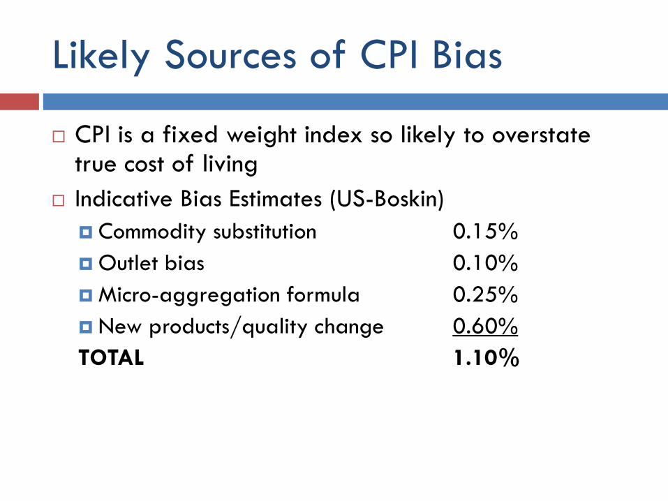
Likely Sources of CPI Bias

CPI is a fixed weight index so likely to overstate true cost of living

Indicative Bias Estimates (US-Boskin)

Commodity substitution 0.15%

Outlet bias 0.10%

Micro-aggregation formula 0.25%

New products/quality change 0.60%

TOTAL 1.10%

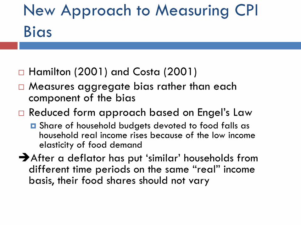
New Approach to Measuring CPI

Bias

Hamilton (2001) and Costa (2001)

Measures aggregate bias rather than each component of the bias

Reduced form approach based on Engel‟s Law Share of household budgets devoted to food falls as

household real income rises because of the low income elasticity of food demand

After a deflator has put „similar‟ households from different time periods on the same “real” income basis, their food shares should not vary

“of all the empirical regularities observed in economic data, Engel‟s Law is probably the best established; indeed it holds not only in the cross-section data where it was first observed, but has often been confirmed in time-series analysis as well.”

(Houthhakker, 1987)

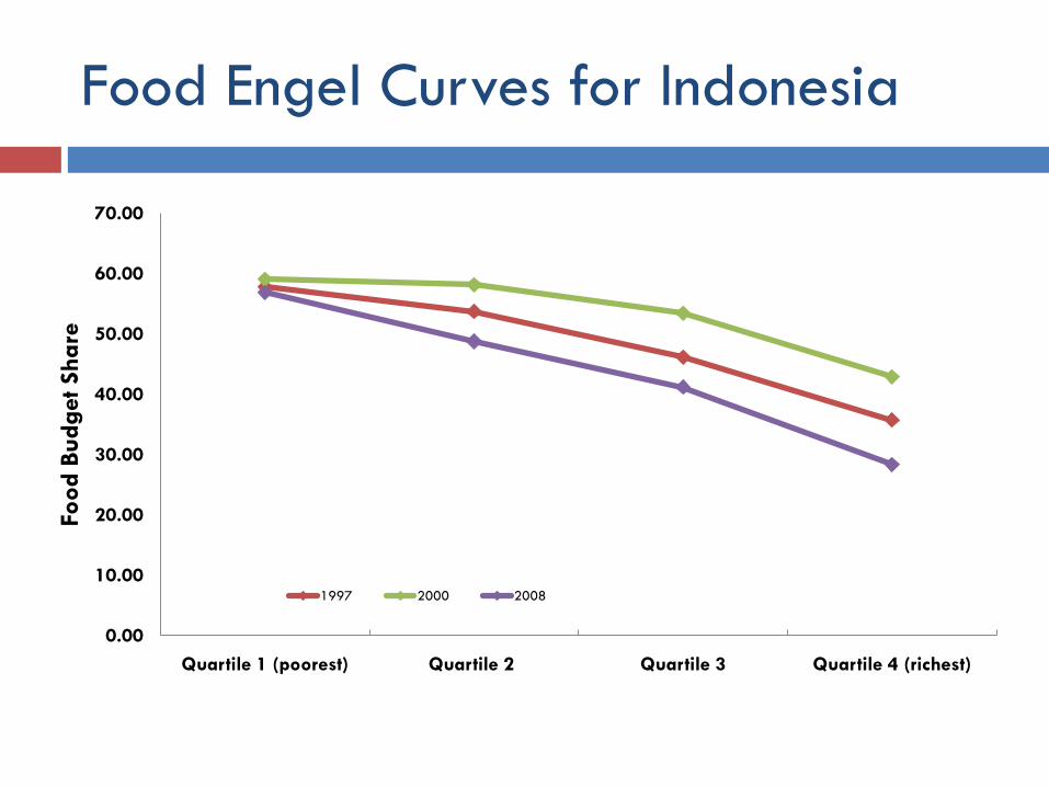
Food Engel Curves for Indonesia

0.00

10.00

20.00

30.00

40.00

50.00

60.00

70.00

Quartile 1 (poorest) Quartile 2 Quartile 3 Quartile 4 (richest)

Foo

d B

ud

get Share

1997 2000 2008

Results of the Engel‟s Law Approach

U.S. (Hamilton, AER, 2001)

Food share fell 4.5 percentage points from 1974 – 1991

Rise in CPI-deflated income explains only 1.5 percentage points

Relative food prices and trends in other variables explain 0.5 percentage points

2.5 percentage points of food share fall unexplained attribute to bias in the CPI

Bias averaged 2.5% per year until 1981, 1% per year thereafter

Canada (Beatty and Larsen, 2005)

Annual bias between 1.3% and 2.9% in the Canadian CPI over 1978 – 2000

Australia (Barrett and Brzozowski, 2010)

Over the 1975/75 – 2003/04, average annual bias of 1%

Results of the Engel‟s Law Approach [Cont‟d]

Russia (Gibson, Stillman and Le, 2008)

CPI bias averaged 1% per month from 1994 – 2001

Just adjusting for bias in household consumption raises

real per capita GDP by 30% in 2001

The transition to the market in Russia may be less

devastating than previously thought

Brazil (Filho and Chamon, 2012)

CPI bias averaged 3% per year from 1988 – 2003

Corrected for bias, the average HH per capita income grew

by 4.5% per year cf 1.5% suggested by the official data

Why study Indonesia?

Beyond BRICS : Indonesia?

Periodically suffered from bouts of high inflation

During the Asian Financial Crisis

In the modern U.S., Canada, Russia, and Brazil, the CPI appears to exaggerate increases in the cost of living. But for Norway and some historical US periods, the bias was negative. Which is it for Indonesia?

This paper presents evidence on bias in the CPI for Indonesia using the Engel Curve method

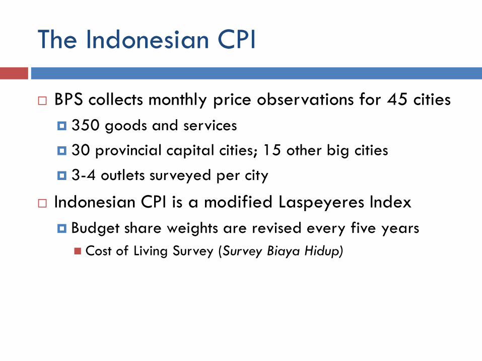
The Indonesian CPI

BPS collects monthly price observations for 45 cities

350 goods and services

30 provincial capital cities; 15 other big cities

3-4 outlets surveyed per city

Indonesian CPI is a modified Laspeyeres Index

Budget share weights are revised every five years

Cost of Living Survey (Survey Biaya Hidup)

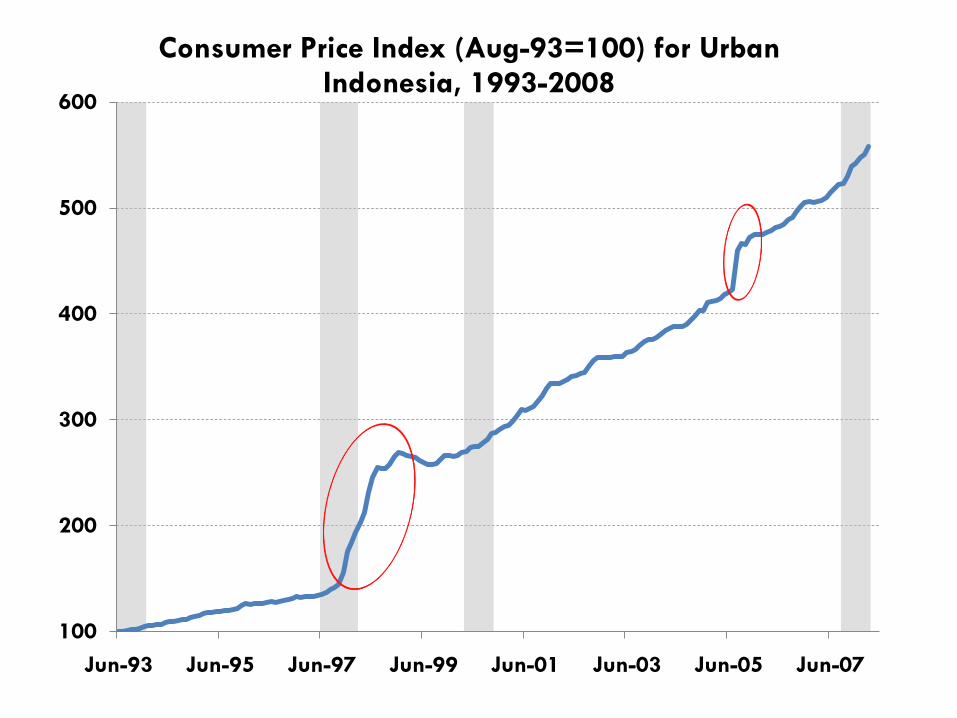
100

200

300

400

500

600

Jun-93 Jun-95 Jun-97 Jun-99 Jun-01 Jun-03 Jun-05 Jun-07

Consumer Price Index (Aug-93=100) for Urban Indonesia, 1993-2008

0.8

1.0

1.2

1.4

1.6

1.8

2.0

Jun-93 Jun-95 Jun-97 Jun-99 Jun-01 Jun-03 Jun-05 Jun-07

Relative Food/NonFood Price Change in Urban Indonesia, 1993-2008

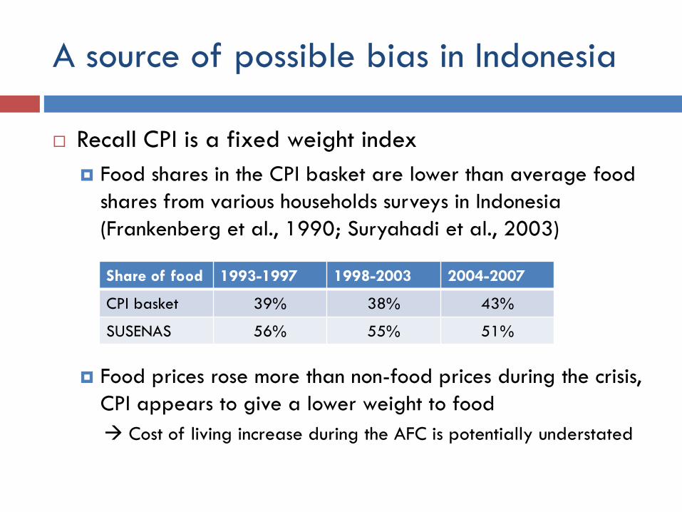
A source of possible bias in Indonesia

Recall CPI is a fixed weight index

Food shares in the CPI basket are lower than average food

shares from various households surveys in Indonesia

(Frankenberg et al., 1990; Suryahadi et al., 2003)

Food prices rose more than non-food prices during the crisis,

CPI appears to give a lower weight to food

Cost of living increase during the AFC is potentially understated

Share of food 1993-1997 1998-2003 2004-2007

CPI basket 39% 38% 43%

SUSENAS 56% 55% 51%

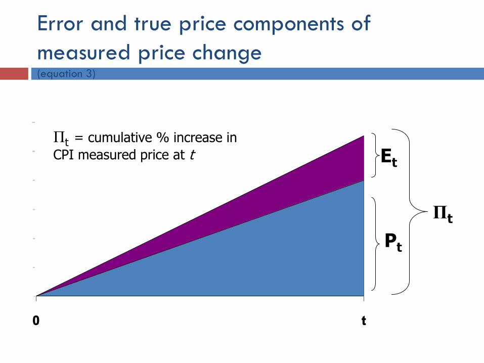
Error and true price components of

measured price change (equation 3)

0

2 0

4 0

6 0

8 0

1 00

1 2 0

0 t

Pt

Et

Πt

Πt = cumulative % increase in

CPI measured price at t

Empirical Framework

With regional variation in Pf/Pnf

Data

Indonesia Family Life Survey (IFLS)

Longitudinal survey

Waves 1 – 4

Wave 1 covered 30,000 individuals in 7,224 households

Low attrition rate

90% of the original target households were re-interview in wave 4

Sample had grown to 13,535 households by wave 4

Collects detailed expenditures and consumption

A one-week recall for food (35) & annual recall for non-foods (25)

Only urban households use here

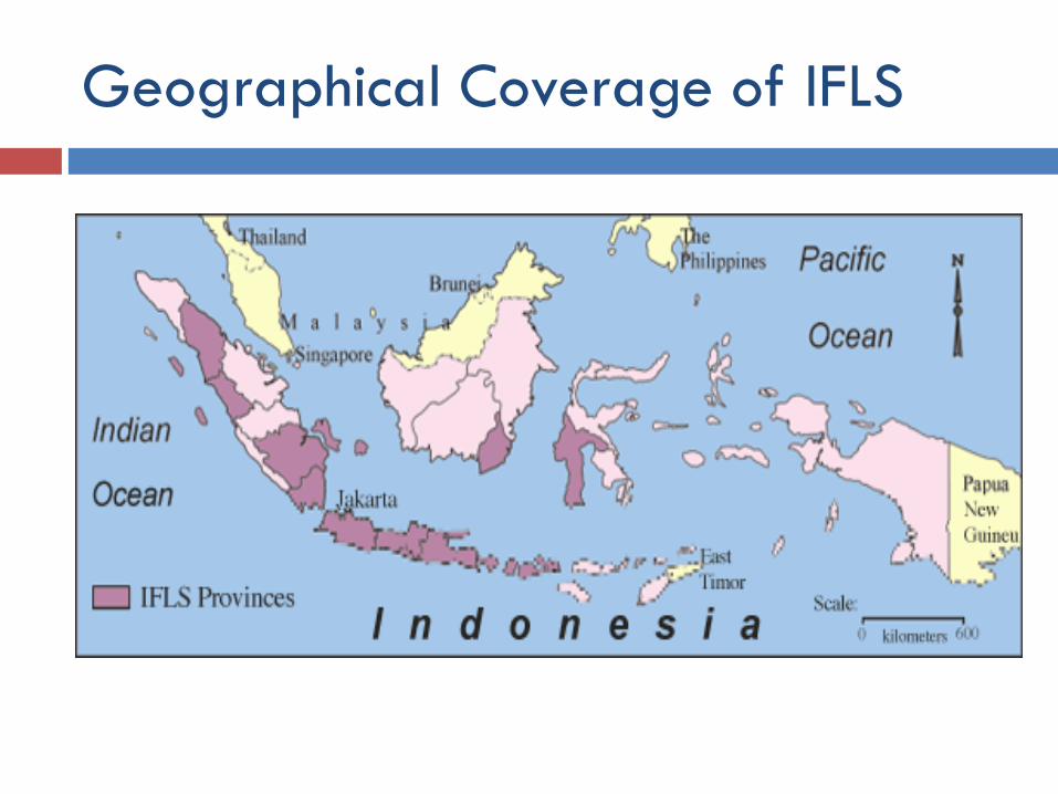
Geographical Coverage of IFLS

Table 1: Descriptive statistics for the sample

Full sample

Wave 1

(1993)

Wave 4

(2007/08)

Mean Std dev Mean Mean

Budget share for food at home 0.404 0.201 0.381 0.293

ln(CPI-deflated total expenditure) 12.835 0.950 12.820 13.220

ln(relative food price)a

0.204 0.187 -0.005 0.328

Budget share for food eaten out 0.053 0.085 0.062 0.044

Demographic variables

ln(household size) 1.599 0.515 1.468 1.874

% of household (HH) 2 years old 2.530 6.519 3.871 1.624

% of HH 3-14 year old boys 10.073 13.435 12.438 7.087

% of HH 15-17 year old boys 9.741 13.197 12.052 6.920

% of HH 3-14 year old girls 3.233 7.457 3.079 2.915

% of HH 15-17 year old girls 3.169 7.496 3.286 2.492

% of HH who are adult males 33.231 17.467 29.713 37.551

Age of household head 48.500 12.353 44.786 52.299

Dummy variables

Head completed secondary school 0.329 0.470 0.330 0.316

Household head is working 0.821 0.384 0.818 0.801

Household head is married 0.804 0.397 0.845 0.770

Female headed-household 0.191 0.393 0.153 0.223

HH engaged in farm-related work 0.131 0.337 0.110 0.161

Muslim household 0.895 0.307 0.883 0.913

Sample size 11,348 3,006 2,642

Estimation approaches

Include split-off households if they stay in an urban

area in the same province in wave 1

Exclude HH with extreme food shares

Restrict HHs where household head between 21 and

75 years old

Multiple estimators used

independent cross-sections vs panel, fe

OLS and IV

Linear vs quadratic income effects

Key Coefficient Values

OLS estimates

Linear Quadratic

ln(CPI-deflated total expenditure) -0.097 -0.190

(29.07)** (3.53)**

[ln(CPI-deflated total

expenditure)]2

0.004

(1.72)+

IFLS wave 2 (08/97--03/98) 0.056 0.057

(8.88)** (8.93)**

IFLS wave 3 (06/00--12/00) 0.070 0.071

(6.92)** (6.97)**

IFLS wave 4 (11/07--05/08) -0.084 -0.083

(8.87)** (8.66)**

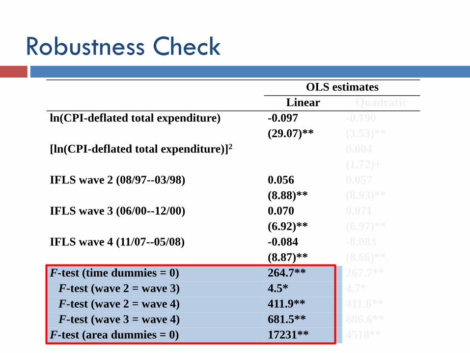
Robustness Check

OLS estimates

Linear Quadratic


(29.07)** (3.53)**

[ln(CPI-deflated total expenditure)]2 0.004

(1.72)+

IFLS wave 2 (08/97--03/98) 0.056 0.057

(8.88)** (8.93)**

IFLS wave 3 (06/00--12/00) 0.070 0.071

(6.92)** (6.97)**

IFLS wave 4 (11/07--05/08) -0.084 -0.083

(8.87)** (8.66)**

F-test (time dummies = 0) 264.7** 267.7**

F-test (wave 2 = wave 3) 4.5* 4.7*

F-test (wave 2 = wave 4) 411.9** 411.6**

F-test (wave 3 = wave 4) 681.5** 686.6**

F-test (area dummies = 0) 17231** 4518**

Robustness Check

OLS estimates

Linear Quadratic


(29.07)** (3.53)**

[ln(CPI-deflated total expenditure)]2 0.004

(1.72)+

IFLS wave 2 (08/97--03/98) 0.056 0.057

(8.88)** (8.93)**

IFLS wave 3 (06/00--12/00) 0.070 0.071

(6.92)** (6.97)**

IFLS wave 4 (11/07--05/08) -0.084 -0.083

(8.87)** (8.66)**


F-test (wave 2 = wave 3) 4.5* 4.7*

F-test (wave 2 = wave 4) 411.9** 411.6**

F-test (wave 3 = wave 4) 681.5** 686.6**


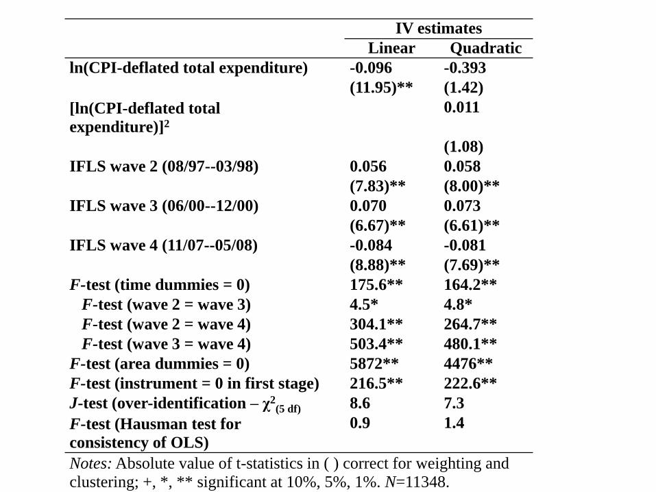
IV estimates

Linear Quadratic


(11.95)** (1.42)

[ln(CPI-deflated total

expenditure)]2

0.011

(1.08)

IFLS wave 2 (08/97--03/98) 0.056 0.058

(7.83)** (8.00)**

IFLS wave 3 (06/00--12/00) 0.070 0.073

(6.67)** (6.61)**

IFLS wave 4 (11/07--05/08) -0.084 -0.081

(8.88)** (7.69)**


F-test (wave 2 = wave 3) 4.5* 4.8*

F-test (wave 2 = wave 4) 304.1** 264.7**

F-test (wave 3 = wave 4) 503.4** 480.1**


F-test (instrument = 0 in first stage) 216.5** 222.6**

J-test (over-identification – χ2(5 df) 8.6 7.3

F-test (Hausman test for

consistency of OLS)

0.9 1.4

Notes: Absolute value of t-statistics in ( ) correct for weighting and clustering; +, *, ** significant at 10%, 5%, 1%. N=11348.

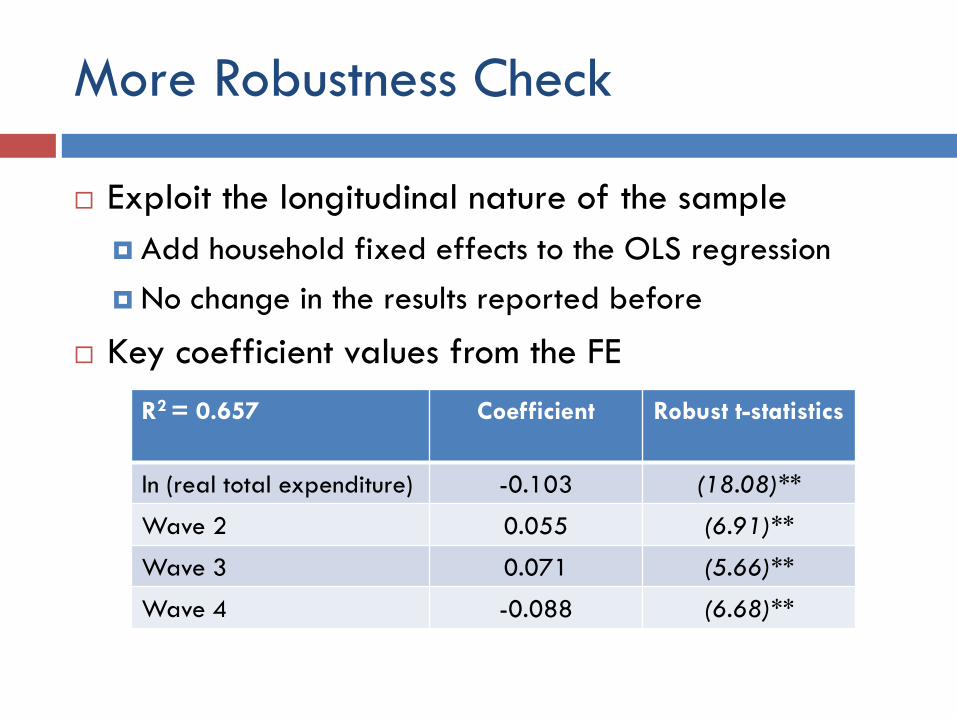
More Robustness Check

Exploit the longitudinal nature of the sample

Add household fixed effects to the OLS regression

No change in the results reported before

Key coefficient values from the FE

R2 = 0.657 Coefficient Robust t-statistics

ln (real total expenditure) -0.103 (18.08)**

Wave 2 0.055 (6.91)**

Wave 3 0.071 (5.66)**

Wave 4 -0.088 (6.68)**

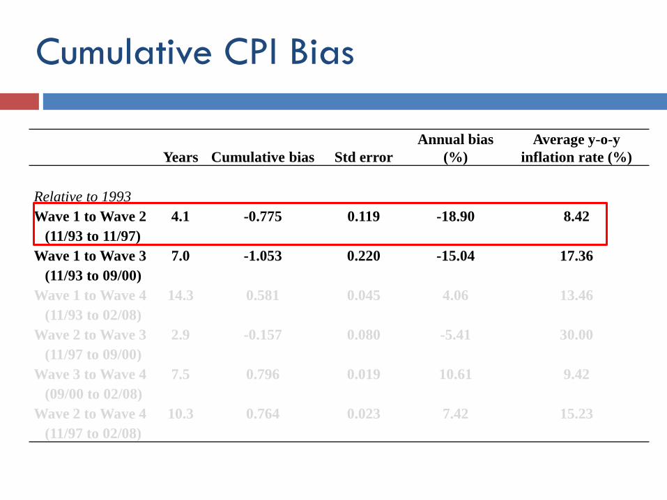
Cumulative CPI Bias

Years Cumulative bias Std error

Annual bias

(%)

Average y-o-y

inflation rate (%)

Relative to 1993

Wave 1 to Wave 2 4.1 -0.775 0.119 -18.90 8.42

(11/93 to 11/97)

Wave 1 to Wave 3 7.0 -1.053 0.220 -15.04 17.36

(11/93 to 09/00)

Wave 1 to Wave 4 14.3 0.581 0.045 4.06 13.46

(11/93 to 02/08)

Wave 2 to Wave 3 2.9 -0.157 0.080 -5.41 30.00

(11/97 to 09/00)

Wave 3 to Wave 4 7.5 0.796 0.019 10.61 9.42

(09/00 to 02/08)

Wave 2 to Wave 4 10.3 0.764 0.023 7.42 15.23

(11/97 to 02/08)

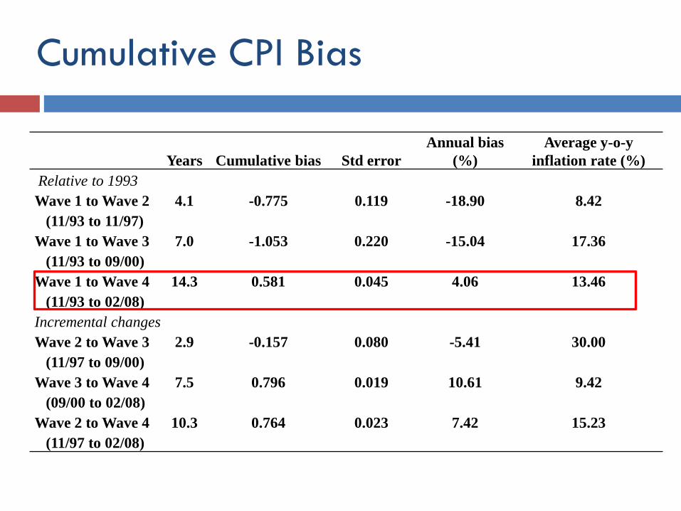
Cumulative CPI Bias

Years Cumulative bias Std error

Annual bias

(%)

Average y-o-y

inflation rate (%)

Relative to 1993

Wave 1 to Wave 2 4.1 -0.775 0.119 -18.90 8.42

(11/93 to 11/97)

Wave 1 to Wave 3 7.0 -1.053 0.220 -15.04 17.36

(11/93 to 09/00)

Wave 1 to Wave 4 14.3 0.581 0.045 4.06 13.46

(11/93 to 02/08)

Incremental changes

Wave 2 to Wave 3 2.9 -0.157 0.080 -5.41 30.00

(11/97 to 09/00)

Wave 3 to Wave 4 7.5 0.796 0.019 10.61 9.42

(09/00 to 02/08)

Wave 2 to Wave 4 10.3 0.764 0.023 7.42 15.23

(11/97 to 02/08)

Conclusions

We need price deflators to assess economic

performance

BUT measuring changes in the cost of living is not easy

Using the Engel curves approach, we found that:

CPI bias was initially negative during the Asian

Financial Crisis, then positive since 2000

Over the entire period of 1993 – 2008, CPI bias

averaged 4 % annually

1/3 of the measured inflation rate

Commodity Substitution Bias

Prices rise faster for some goods than others

Consumers will tend to substitute away from goods

whose price has risen

CPI weights each price change according to the

expenditure weights in the base period

Put too much weight on items whose prices are rising

fastest

Problem is reduced by having more frequent reviews of

weight

Outlet Bias (e.g. The Wal-Mart Effect)

Prices rise faster in some retail outlets than others

Consumers switch toward outlets with more stable (and lower) prices (Wal-Mart in the U.S.)

A fixed sample of outlets for CPI price quotes over-represents those where prices rise rapidly and under-represents those where prices rise more slowly

Even if discount outlets with more stable prices are rotated into the CPI sample, some statistics agencies treat the lower price as a lower quality of service rather than a genuine price reduction

If this were true, consumers would be indifferent between discounters and traditional department stores, and would be no change in market share

Formula Bias

Formula needed to aggregate individual price quotations

Calculating price change from each outlet and averaging can cause a systematic upward bias

Why? Treats each price quote as equally important, but consumers will switch away from the outlet (or brand) with rapidly rising prices

Either a geometric mean of ratios or the ratio of mean prices gives lower average price change

2011 2012 Ratio

Store A $3.50 $4.20 1.2

Store B $2.50 $3.50 1.4

Mean $3.00 $3.85

Average

of ratios

1.30

Ratio of

means

1.28

Quality Change Bias

If a product improves in quality, consumers get more

for their money so the true price rise is less than the

apparent price rise

E.g. Windows Vista vs Windows7

Statistics agencies sometimes attempt to adjust for

the improved characteristics of products (“hedonic

regressions‟) but this is incomplete and does not

capture all of the quality change

Documents

Using Engel Curves to Measure CPI Bias for Indonesia