Using DERIVE 6.1 To Generate

DNA Fractal Representations

Joel Jeffrey’s Chaos Game

Representation, Genomic

Signatures, and Aligning Sequences

L. Carl Leinbach

Gettysburg College

Gettysburg, PA USA

leinbach@gettysburg.edu

The Chaos Game

The Chaos Game (Jeffrey’s name) is basically an Iterated Function System

dependent upon points arranged in some geometric configuration. The best

known example is that of Sierpinski’s Triangle.

In this case, the point configuration is the vertices of a triangle located in the

plane, say at vertices, v1 = (0,0), v2 = (1/2, 1), and v3 = (1,0). The sequence of

points (xi, yi) is then chosen with (x0, y0 ) = (1/2, 1/ 2) and

𝑥𝑖 = 𝑥𝑖−1 + 𝑣𝑟𝑖+ 𝑥𝑖−1

2

for I = 1, 2, . . .

𝑦𝑖= 𝑦𝑖−1 + 𝑣𝑟2 +𝑦𝑖−1

2

At each step vr is randomly chosen from among the vertices v1, v2, and v3.

This process is easily programmed in DERIVE and the result graphed.

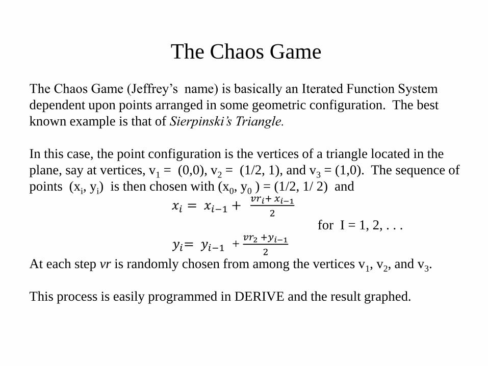
Sierpinski(T, n, i, j, k, X, Y) ≔ Prog i ≔ 1 P ≔ [1/2, 1/2] X ≔ [P↓1] Y ≔ [P↓2] Loop i ≔ i + 1 If i > n RETURN VECTOR([X↓j, Y↓j], j, 1, n) k ≔ RANDOM(3) + 1 P ≔ [(P↓1 + T↓k↓1)/2, (P↓2 + T↓k↓2)/2] X ≔ INSERT(P↓1, X, i) Y ≔ INSERT(P↓2, Y, i)

Below is an example of a typical program for constructing the Sierpinski

Triangle and the result of the program after 10,000 iterations. The result is

always the same, independent of the choice of the starting point and, remarkably,

the quality of the pseudo-random number generator picking the target vertex.

Sierpinski(T, 10000)

The Birth of the Chaos Game Representation

In his 1990 article in Nucleic Acids Research , Jeffrey noted that if an iterated function

system using the same “Chaos Game” strategy is applied to figures with 5, 6, 7 as well

as three vertices, the result is the same independent of the quality of the random number

generator. However, with 8 vertices, and to a lesser extent 4 vertices, the result was

dramatically different.

Using a good random number generator with 8 vertices, the result of the Chaos Game

was an almost uniformly filled octagon. When the game was played using the random

number generator from Turbo Pascal 3.0 (a notoriously bad generator) the result was

an elaborate pattern generating a circle within a circle and the circles connected by 8

spidery lines. The DOS Basic v2.1 function RND produced no visible pattern at all for

8 vertices.

This experience, according to Jeffrey’s account, led him to the conclusion that the

Chaos Game can display certain kinds of non randomness visually. In particular,

patterns in a four vertex Chaos Game having the vertices labeled starting at the bottom

left and proceeding clockwise with the letters, “A”, “C” , “G”, and “T” could be

observed by controlling the moves with successive letters in a particular DNA sequence.

He called the resulting pattern the “Chaos Game Representation” of the sequence.

An All Too Brrief

Introduction to DNA

Much work preceded the spectacular 1953 announcement of the

double helical structure of DNA by Watson and Crick. Nucleic

Acid was known prior to 1820. DNA was first identified in 1869

and, simultaneously Mendel was doing his pioneering research in

genetics. In the 1940’s Linus Pauling predicted a three

dimensional structure for the DNA molecule. The X-ray

diffraction work of Rosalind Franklin and Maurice Wilkins

played a major role in the Watson–Crick discovery.

DNA consists chains made up from four nucleotides,

two Purines:

Adenine - A

Guanine - G

and two Pyrimidines:

Thymine – T

Cytosine - C

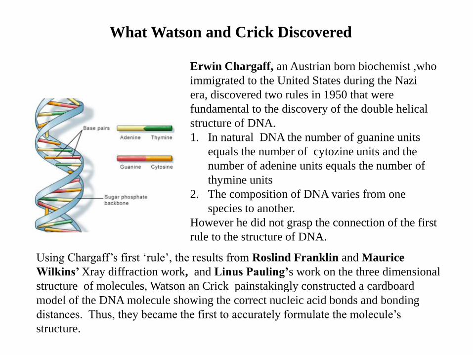
What Watson and Crick Discovered

Erwin Chargaff, an Austrian born biochemist ,who

immigrated to the United States during the Nazi

era, discovered two rules in 1950 that were

fundamental to the discovery of the double helical

structure of DNA.

1. In natural DNA the number of guanine units

equals the number of cytozine units and the

number of adenine units equals the number of

thymine units

2. The composition of DNA varies from one

species to another.

However he did not grasp the connection of the first

rule to the structure of DNA.

Using Chargaff’s first ‘rule’, the results from Roslind Franklin and Maurice

Wilkins’ Xray diffraction work, and Linus Pauling’s work on the three dimensional

structure of molecules, Watson an Crick painstakingly constructed a cardboard

model of the DNA molecule showing the correct nucleic acid bonds and bonding

distances. Thus, they became the first to accurately formulate the molecule’s

structure.

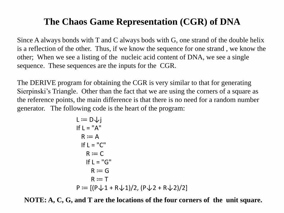
The Chaos Game Representation (CGR) of DNA

Since A always bonds with T and C always bods with G, one strand of the double helix

is a reflection of the other. Thus, if we know the sequence for one strand , we know the

other; When we see a listing of the nucleic acid content of DNA, we see a single

sequence. These sequences are the inputs for the CGR.

The DERIVE program for obtaining the CGR is very similar to that for generating

Sierpinski’s Triangle. Other than the fact that we are using the corners of a square as

the reference points, the main difference is that there is no need for a random number

generator. The following code is the heart of the program:

L ≔ D↓j If L = "A" R ≔ A If L = "C" R ≔ C If L = "G" R ≔ G R ≔ T P ≔ [(P↓1 + R↓1)/2, (P↓2 + R↓2)/2]

NOTE: A, C, G, and T are the locations of the four corners of the unit square.

C

A T

G

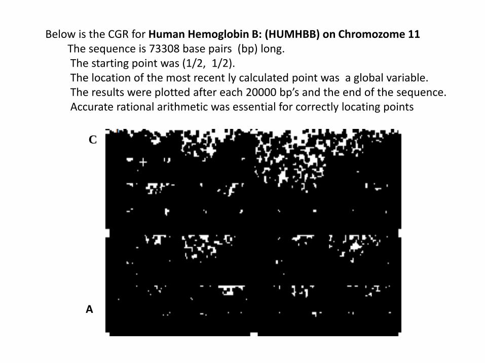
Below is the CGR for Human Hemoglobin B: (HUMHBB) on Chromozome 11 The sequence is 73308 base pairs (bp) long. The starting point was (1/2, 1/2). The location of the most recent ly calculated point was a global variable. The results were plotted after each 20000 bp’s and the end of the sequence. Accurate rational arithmetic was essential for correctly locating points

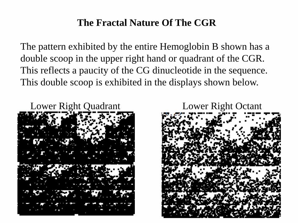
The Fractal Nature Of The CGR

The pattern exhibited by the entire Hemoglobin B shown has a

double scoop in the upper right hand or quadrant of the CGR.

This reflects a paucity of the CG dinucleotide in the sequence.

This double scoop is exhibited in the displays shown below.

Lower Right Quadrant Lower Right Octant

The Shape of the CGR

For Any Sequence Of Reasonable Length

If we choose any two base pairs that are at least a few thousand positions apart in the

sequence, we will see the same basic pattern exhibited. Shown below is the CGR of

the HUMHBB sequence between bp 53000 and 58271

According to Jeffrey the double scoop shape is has been found only in DNA sequences

for vertebrates and in the human and chimpanzee HIV virus. And ,it can be used to

classify these viruses.

Another Example of the Fractal Behavior

To illustrate that the phenomenon observed for the Human

Hemoglobin B is not a one time occurrence, The CGR was applied

to Gordonia otitidis, a pathogen that can cause blood infections. On

the left is the complete sequence for the Gordonia and on the right is

a partial sequence involving 2500 base pairs. Note that we do not

have the double scoops in the CG region; however there is a paucity

in the AT region.

Godonia otitdis – 9421 bp CGR for bp 3241 to 5678

Jeffrey’s Observations

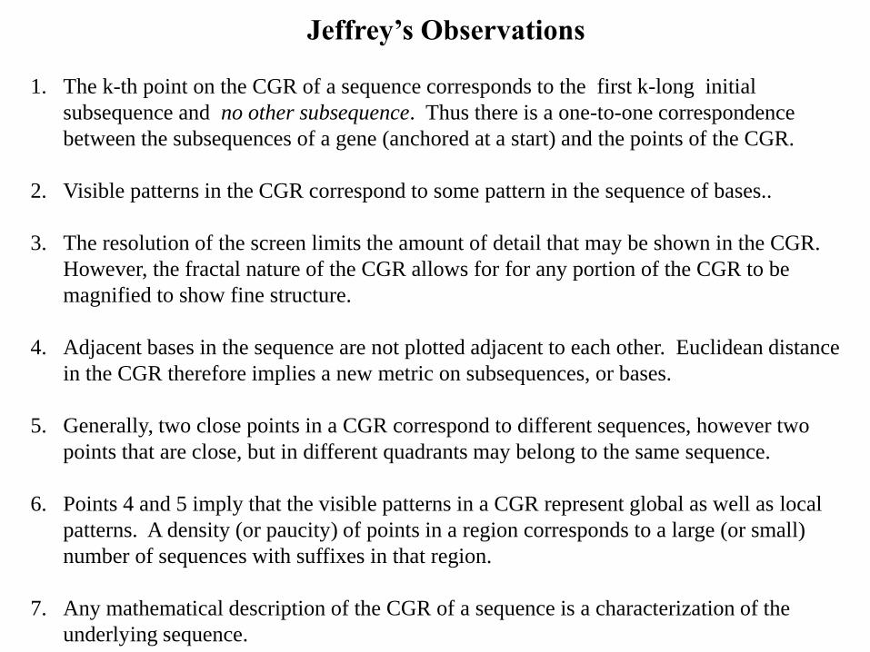
1. The k-th point on the CGR of a sequence corresponds to the first k-long initial

subsequence and no other subsequence. Thus there is a one-to-one correspondence

between the subsequences of a gene (anchored at a start) and the points of the CGR.

2. Visible patterns in the CGR correspond to some pattern in the sequence of bases..

3. The resolution of the screen limits the amount of detail that may be shown in the CGR.

However, the fractal nature of the CGR allows for for any portion of the CGR to be

magnified to show fine structure.

4. Adjacent bases in the sequence are not plotted adjacent to each other. Euclidean distance

in the CGR therefore implies a new metric on subsequences, or bases.

5. Generally, two close points in a CGR correspond to different sequences, however two

points that are close, but in different quadrants may belong to the same sequence.

6. Points 4 and 5 imply that the visible patterns in a CGR represent global as well as local

patterns. A density (or paucity) of points in a region corresponds to a large (or small)

number of sequences with suffixes in that region.

7. Any mathematical description of the CGR of a sequence is a characterization of the

underlying sequence.

Jeffrey’s Theorem

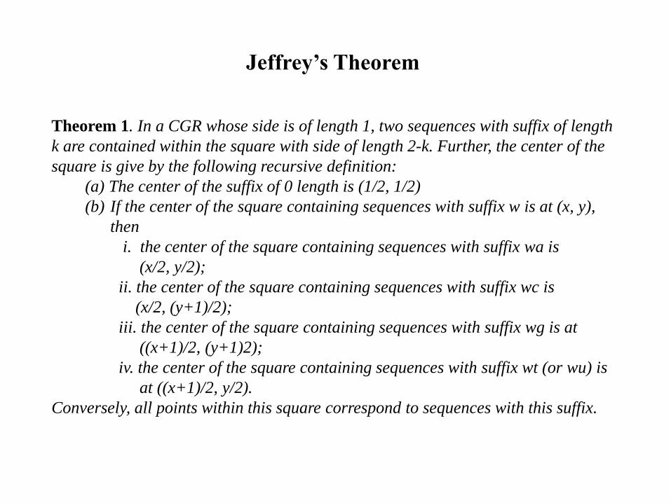
Theorem 1. In a CGR whose side is of length 1, two sequences with suffix of length

k are contained within the square with side of length 2-k. Further, the center of the

square is give by the following recursive definition:

(a) The center of the suffix of 0 length is (1/2, 1/2)

(b) If the center of the square containing sequences with suffix w is at (x, y),

then

i. the center of the square containing sequences with suffix wa is

(x/2, y/2);

ii. the center of the square containing sequences with suffix wc is

(x/2, (y+1)/2);

iii. the center of the square containing sequences with suffix wg is at

((x+1)/2, (y+1)2);

iv. the center of the square containing sequences with suffix wt (or wu) is

at ((x+1)/2, y/2).

Conversely, all points within this square correspond to sequences with this suffix.

Illustrating Jeffrey’s Theorem

Starting at the center of the square with coordinates A = [0,0], C = [0,1], G = [1,1]

and T = [1,0], trace each successive nucleotide base pair in th e string. Each

point in the plot represents the entire sequence to that point. Also note the

position of the G term is closer to the first T term than it is to C.

G GC GCT GCTT

GCTTA

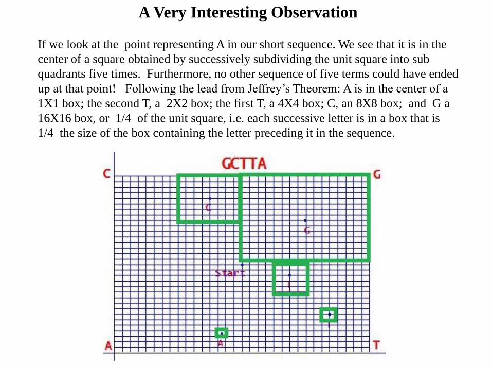
A Very Interesting Observation

If we look at the point representing A in our short sequence. We see that it is in the

center of a square obtained by successively subdividing the unit square into sub

quadrants five times. Furthermore, no other sequence of five terms could have ended

up at that point! Following the lead from Jeffrey’s Theorem: A is in the center of a

1X1 box; the second T, a 2X2 box; the first T, a 4X4 box; C, an 8X8 box; and G a

16X16 box, or 1/4 of the unit square, i.e. each successive letter is in a box that is

1/4 the size of the box containing the letter preceding it in the sequence.

An Illustration of The

Independence of Starting Point

On the CGR Graph below the sequence GCTTA was plotted from three different

initial points: [1/2, 1/2] (black), [2/3, 5/9] (red), and [9/13, 13/15] (blue). Note that

all three ending points ended in the same 1/32 X 1/32 region of the graph.

Towards Constructing a Genomic Signature

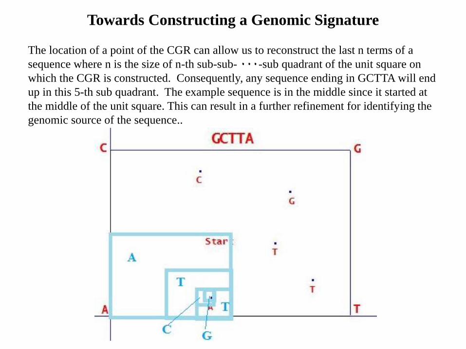
The location of a point of the CGR can allow us to reconstruct the last n terms of a

sequence where n is the size of n-th sub-sub- ٠٠٠-sub quadrant of the unit square on

which the CGR is constructed. Consequently, any sequence ending in GCTTA will end

up in this 5-th sub quadrant. The example sequence is in the middle since it started at

the middle of the unit square. This can result in a further refinement for identifying the

genomic source of the sequence..

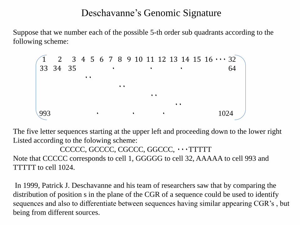
Deschavanne’s Genomic Signature

Suppose that we number each of the possible 5-th order sub quadrants according to the

following scheme:

1 2 3 4 5 6 7 8 9 10 11 12 13 14 15 16 ٠٠٠ 32 33 34 35 ٠ ٠ ٠ 64

٠٠

٠٠ ٠٠ ٠٠

993 ٠ ٠ ٠ 1024

The five letter sequences starting at the upper left and proceeding down to the lower right

Listed according to the folowing scheme:

CCCCC, GCCCC, CGCCC, GGCCC, ٠٠٠TTTTT

Note that CCCCC corresponds to cell 1, GGGGG to cell 32, AAAAA to cell 993 and

TTTTT to cell 1024.

In 1999, Patrick J. Deschavanne and his team of researchers saw that by comparing the

distribution of position s in the plane of the CGR of a sequence could be used to identify

sequences and also to differentiate between sequences having similar appearing CGR’s , but

being from different sources.

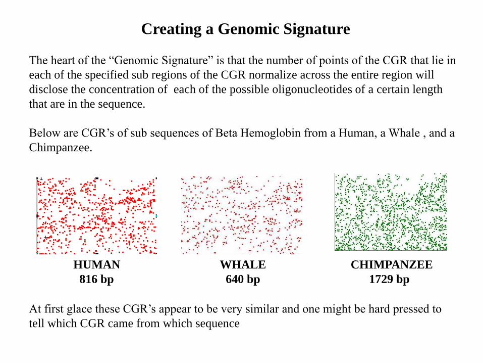
Creating a Genomic Signature

The heart of the “Genomic Signature” is that the number of points of the CGR that lie in

each of the specified sub regions of the CGR normalize across the entire region will

disclose the concentration of each of the possible oligonucleotides of a certain length

that are in the sequence.

Below are CGR’s of sub sequences of Beta Hemoglobin from a Human, a Whale , and a

Chimpanzee.

HUMAN WHALE CHIMPANZEE

816 bp 640 bp 1729 bp

At first glace these CGR’s appear to be very similar and one might be hard pressed to

tell which CGR came from which sequence

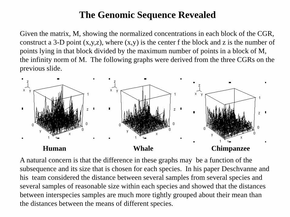
The Genomic Sequence Revealed Given the matrix, M, showing the normalized concentrations in each block of the CGR,

construct a 3-D point (x,y,z), where (x,y) is the center f the block and z is the number of

points lying in that block divided by the maximum number of points in a block of M,

the infinity norm of M. The following graphs were derived from the three CGRs on the

previous slide.

Human Whale Chimpanzee

A natural concern is that the difference in these graphs may be a function of the

subsequence and its size that is chosen for each species. In his paper Deschvanne and

his team considered the distance between several samples from several species and

several samples of reasonable size within each species and showed that the distances

between interspecies samples are much more tightly grouped about their mean than

the distances between the means of different species.

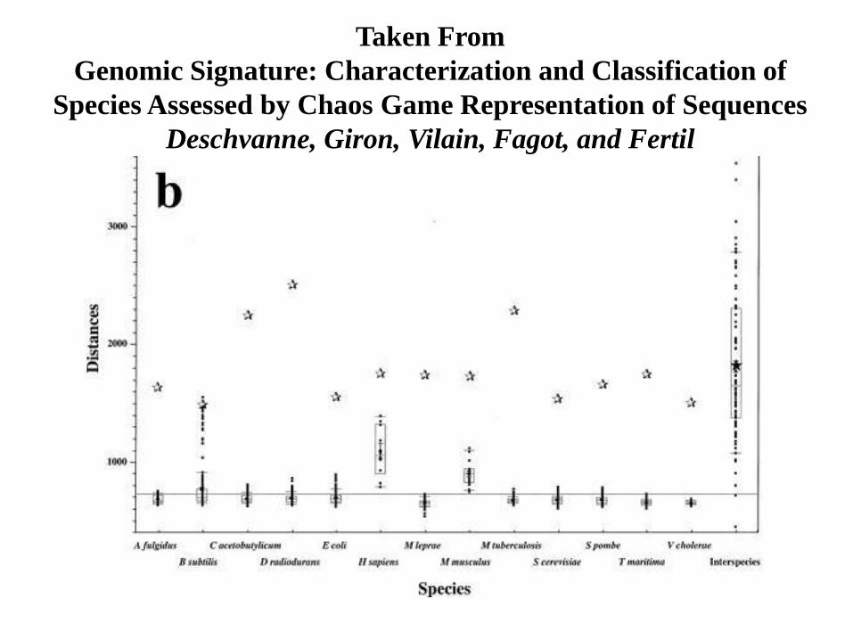
Taken From

Genomic Signature: Characterization and Classification of

Species Assessed by Chaos Game Representation of Sequences

Deschvanne, Giron, Vilain, Fagot, and Fertil

Sequence Homology Why Sequence Alignment is Important

DNA sequences develop from pre-existing sequences instead of being invented by nature

from scratch . This fact makes sequence alignment an important part of biological

research. If the DNA is taken from an area which has a function or structure from a

known sequence, then , if the sequences exhibit regions of similarity, then it is possible

that the surce f the new sequence will exhibit similar structure or function. When a match

occurs, we say the old and the new sequence are homologous.

At this point we will look for sequence similarity, a first step towards sequence homology.

Several tools exist and are publically available to researchers. The most commonly used

both for DNA and protein sequences is called BLAST (Basic Linear Alignment Tool)

developed by Stephan Altschul, Warren Gish, and David Lipman of the National Center for Biotechnical Information.. It looks for short portions of each sequence that are identical and then stretches in each direction and looks for a good alignment.

The identical sub sequences are called “conserved sequences.” We will show how some

practitioners in the biotechnical field are uing Jeffrey’a CGR as a means of finding

conserved sequences.

A DERIVE Program

For Finding Conserved Sequences

It has been noted that if two CGR points reside in the same block of the 1024 block of a

32 X 32 grid imposed upon the CGR they are the result of mapping the exact same six

letter sequence of the DNA alphabet. The problem is one of finding a strategy for

quickly finding the box in which a point of the CGR resides. We circumvent this point

by saying that since the box is 1

64 X

1

64 , their l1norm of the distance between the two

points in the box is at most 1

32 . We will use a much stricter criterion of considering

only points that lie within 1

256 units of each other. This criterion is not “fool proof”, but

gives a good start for

the search:

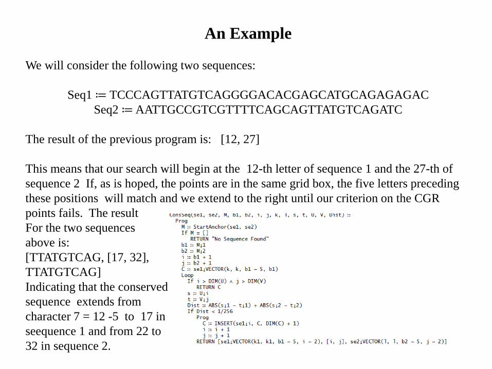
An Example

We will consider the following two sequences:

Seq1 ≔ TCCCAGTTATGTCAGGGGACACGAGCATGCAGAGAGAC

Seq2 ≔ AATTGCCGTCGTTTTCAGCAGTTATGTCAGATC

The result of the previous program is: [12, 27]

This means that our search will begin at the 12-th letter of sequence 1 and the 27-th of

sequence 2 If, as is hoped, the points are in the same grid box, the five letters preceding

these positions will match and we extend to the right until our criterion on the CGR

points fails. The result

For the two sequences

above is:

[TTATGTCAG, [17, 32],

TTATGTCAG]

Indicating that the conserved

sequence extends from

character 7 = 12 -5 to 17 in

seequence 1 and from 22 to

32 in sequence 2.

Shot Gunning The Genome

The DNA making up the human genome is estimated to be about 3.2 Mb in

size. Only about 1.5% of this total is protein coding DNA The rest is made

up of other components; non coding RNA genes, regulatory sequences,

introns, non coding DNA (aka junk DNA).

To fully sequence the human genome in one shot would be an impossible

task. In the late 1940’s , before DNA structure was even known, Sanger was

awarded a Nobel Prize for determining the amino acid sequence of insulin.

He digested insulin in enzymes that broke up the sequence and was able to

sequence the short sequences rather easily. Then since the fragments

overlapped, he was able (no small task) to put the puzzle back together. In

1974, Russian scientist, Andrey Mirzabekov, whiole visiting Harvard found a

way to selectively break DNA at A and G. Later Allan Maxam and Walter

Gilbert found a method to break DNA at every C and T. The short sequences

could be sequenced and then using combinatorics algorithms, be put back

together. This is known as shotgunning.

A Small Example

Of Shot Gunning

The following three sequences were shot gunned from a protein sequnce.

sg1 ≔ GGATCGTCGTCG

sg2 ≔ CGTCGTCGAACAATG

sg3 ≔ CGAACAATGTCGGA

Using the Derive program we are able to solve this very simple example.

First we try sequence 1 and sequence 2

ConsSeq(sg1, sg2)

[CGTCG, [14, 10], CGTCG]

Indeed there is overlap and it occurs at the end of sequence 1 and beginning of sequence

2. However, we still need to check if there is also overlap between seqquence 1 and 3.

ConsSeq(sg1, sg3)

No Sequence Found

So now what about 2 and 3?

ConsSeq(sg3, sg2)

[AACAA, [10, 15], AACAA]

Here we see one of the weaknesses of the heuristic in determining the same block of the

CGR and also the fact that we are dealing with the end of one sequence and the

beginning of another. The program missed th e beginning CG and final TG. There is

still work to be done! – Next time.

Why CAS? Recovery:

Each point of the CGR is the history of the sequence up to that point. Given the

simple nature of the IFS (Iterrated Function System) used to generate the CGR, the

sequence can be completely recovered from the position of the point and the position of

the starting point. A finite word length decimal approximation will quickly loose this

accuracy. Rational arithmetic of the CAS does not have this restriction.

Quoting from Almeida: “The nucleotide sequence can (also) be recovered from the

CGR coordinate, where the the number of the bases resolved is a function of the

resolution of the CGR coordinates.

Sequence Comparison:

We use a grid of size 2𝑛 𝑋 2𝑛 and store the location of the n-length oligonucleotide

sequence represented by the corresponding grid box containing the CGR points from

the sequences under comparison and then extend then extend the sequence as far as

possible within each sequence. Thus, the CGR jump starts the comparison procedure.

In this paper oligonucleotide of length 6 were used.

Quoting from Joseph: “For long identical sequence segments, the minimum value of

the distance value may go below the minimum possible floating point variable… in

double precision the variable becomes zero when the length of identical segments is

greater than 64.”

References

1. Almeida J. S., Carrico J. A., Maretzek A., Nobel P. A. and Fletcher M., “Analysis of

Genomic Sequences by Chaos Game Representation, Bioinformatics, v. 17, no. 4,

2001, pp 429 – 437

2. Deschavanne P. J., Giron P., Vilain J., Fagot G., and Fertil B., “Genomic Signature:

Characterization and Classification by Chaos Game Representation of Sequences” ,

Molecular Biology and Evolution, http://mbe.oxfordjournals.org/ Stanley Sawer,

reviewing editor, June 1999

3. Isaev, A., Introduction to Mathematical Methods in Bioinformatics, Springer, Berlin,

2004

4. Jeffrey, H. J., “Chaos game Representation of Gene Structure”, Nucleic Acids

Research,1 v 18, no, 8, 1990

5. Jones N. C. and Pevsner P. A., An Introduction to Bioinformatics Algorithms, The

MIT Press, Cambridge, Mass., 2004

6. Joseph J. and Sasikumar, R., “Chaos Game Representation of Whole Genomes”,

BioMed Central (Open Access), 10 pages, May, 2006

7. Pevsner, P., Computational Molecular Biology, An Algoritmic Approach, The MIT

Press. Cambridge, Mass., 2000, (Second Printing), 2001