Using Decision Trees to Predict Student Placement and Course Success

CAIR ConferenceNovember 21, 2014

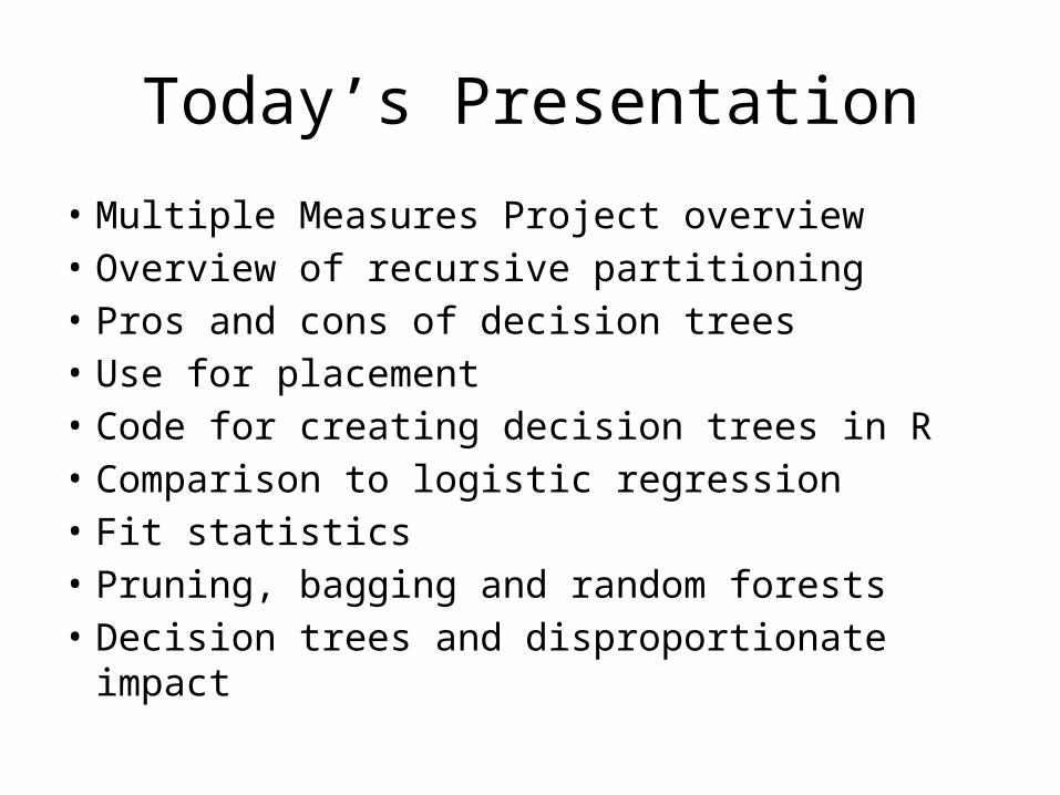
Today’s Presentation

• Multiple Measures Project overview• Overview of recursive partitioning• Pros and cons of decision trees• Use for placement • Code for creating decision trees in R• Comparison to logistic regression• Fit statistics• Pruning, bagging and random forests• Decision trees and disproportionate impact

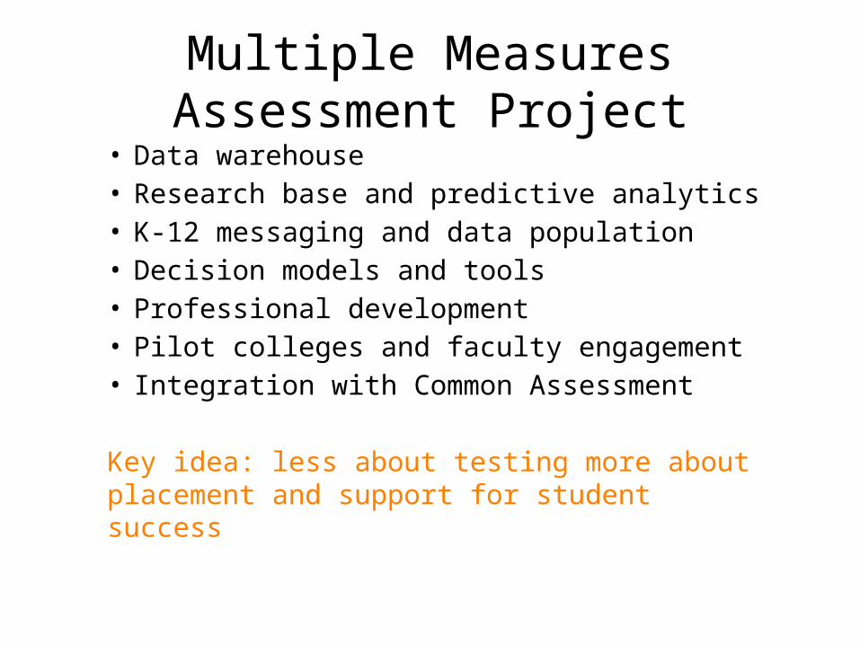
Multiple Measures Assessment Project• Data warehouse• Research base and predictive analytics• K-12 messaging and data population• Decision models and tools • Professional development• Pilot colleges and faculty engagement• Integration with Common Assessment

Key idea: less about testing more about placement and support for student success

Data Warehouse for MMAPData in place…• K-12 transcript data• CST, EAP and CAHSEE• Accuplacer• CCCApply• MIS• Other College Board assessments• Local assessments

Coming soon…• Compass• Common Assessment and SBAC

5

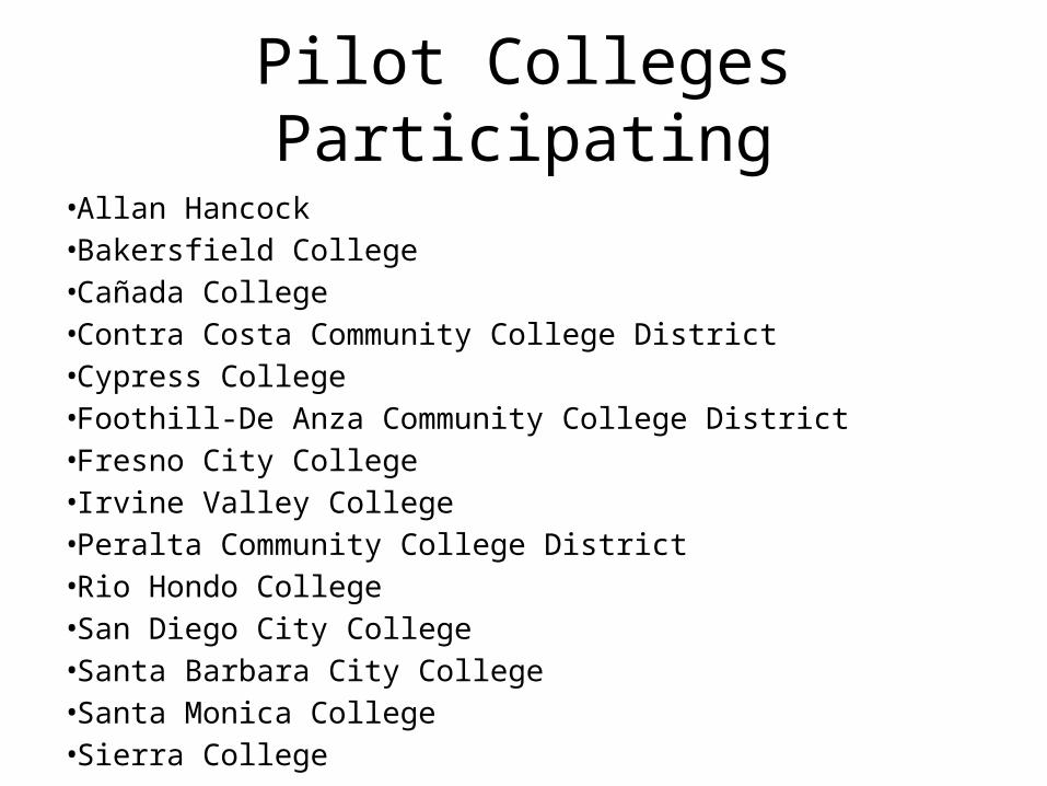
Pilot Colleges Participating• Allan Hancock• Bakersfield College• Cañada College• Contra Costa Community College District • Cypress College• Foothill-De Anza Community College District • Fresno City College• Irvine Valley College• Peralta Community College District• Rio Hondo College• San Diego City College• Santa Barbara City College• Santa Monica College• Sierra College

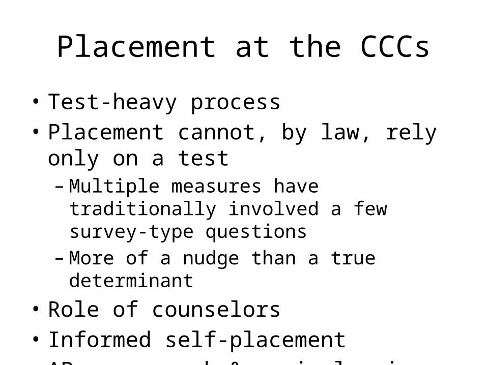
Placement at the CCCs

• Test-heavy process• Placement cannot, by law, rely only on a test– Multiple measures have traditionally involved a

few survey-type questions– More of a nudge than a true determinant

• Role of counselors• Informed self-placement• AP coursework & equivalencies

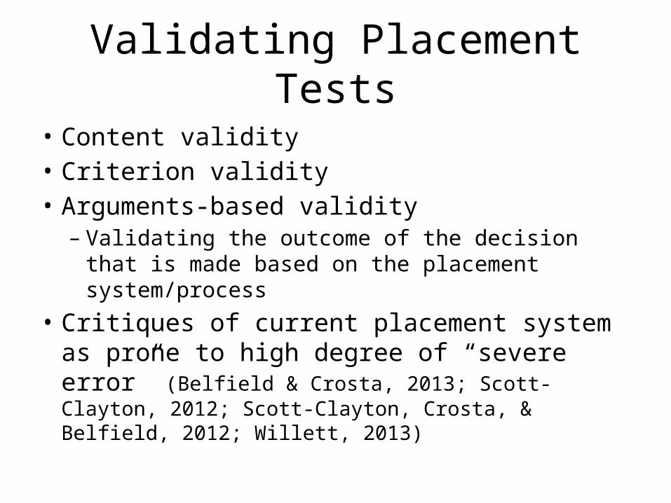
Validating Placement Tests

• Content validity• Criterion validity• Arguments-based validity– Validating the outcome of the decision that is

made based on the placement system/process• Critiques of current placement system as

prone to high degree of “severe error” (Belfield & Crosta, 2013; Scott-Clayton, 2012; Scott-Clayton, Crosta, & Belfield, 2012; Willett, 2013)

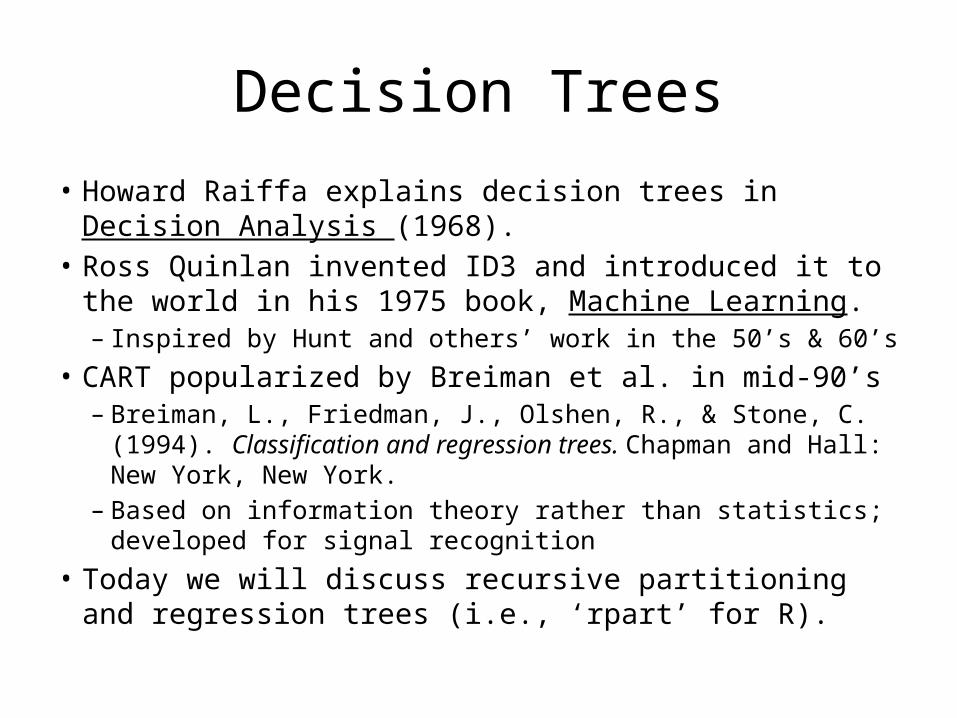
Decision Trees

• Howard Raiffa explains decision trees in Decision Analysis (1968).

• Ross Quinlan invented ID3 and introduced it to the world in his 1975 book, Machine Learning.– Inspired by Hunt and others’ work in the 50’s & 60’s

• CART popularized by Breiman et al. in mid-90’s– Breiman, L., Friedman, J., Olshen, R., & Stone, C. (1994).

Classification and regression trees. Chapman and Hall: New York, New York.

– Based on information theory rather than statistics; developed for signal recognition

• Today we will discuss recursive partitioning and regression trees (i.e., ‘rpart’ for R).

Dog Decision Tree

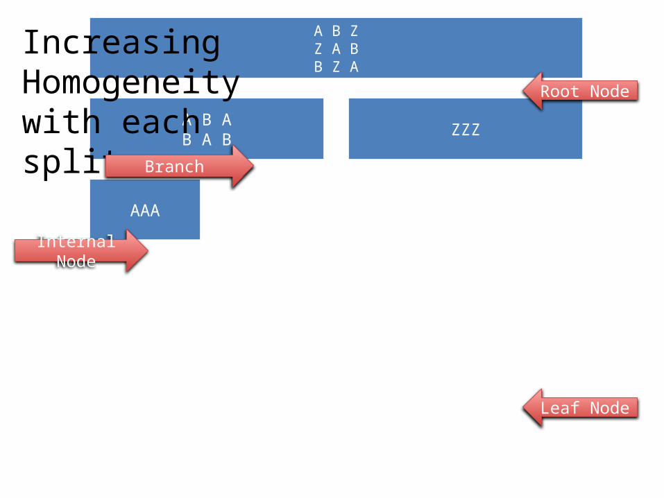
A B ZZ A BB Z A

A B AB A B

AAA

ZZZ

Increasing Homogeneity with each split

Branch

Internal Node

Leaf Node

Root Node

𝐷=1−∑𝑖=1

𝑛

𝑝𝑖2

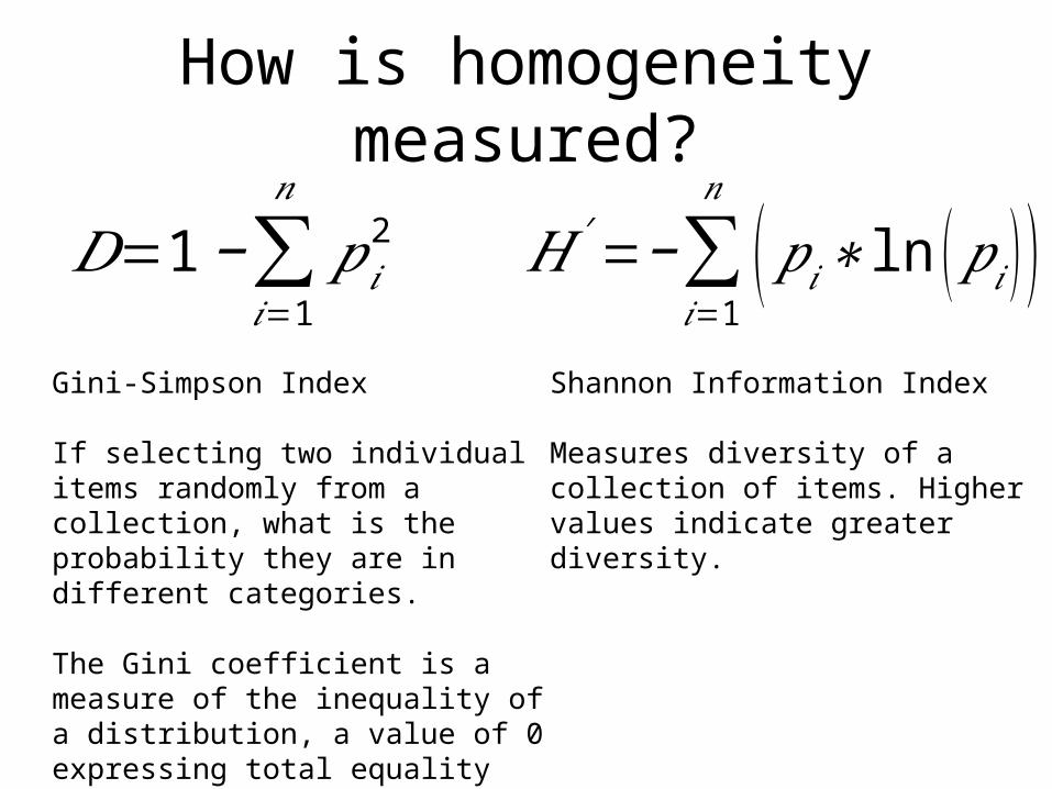
How is homogeneity measured?

Gini-Simpson Index

If selecting two individual items randomly from a collection, what is the probability they are in different categories.

The Gini coefficient is a measure of the inequality of a distribution, a value of 0 expressing total equality and a value of 1 maximal inequality.

𝐻 ′=−∑𝑖=1

𝑛

(𝑝𝑖∗ ln (𝑝𝑖 ))Shannon Information Index

Measures diversity of a collection of items. Higher values indicate greater diversity.

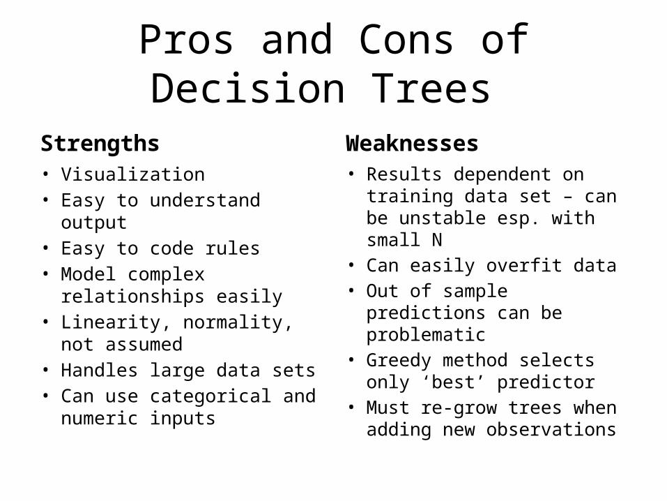
Pros and Cons of Decision Trees

Strengths• Visualization• Easy to understand output• Easy to code rules• Model complex relationships

easily• Linearity, normality, not

assumed • Handles large data sets• Can use categorical and

numeric inputs

Weaknesses• Results dependent on

training data set – can be unstable esp. with small N

• Can easily overfit data• Out of sample predictions

can be problematic• Greedy method selects only

‘best’ predictor• Must re-grow trees when

adding new observations

http://www-users.cs.umn.edu/~kumar/dmbook/ch4.pdf

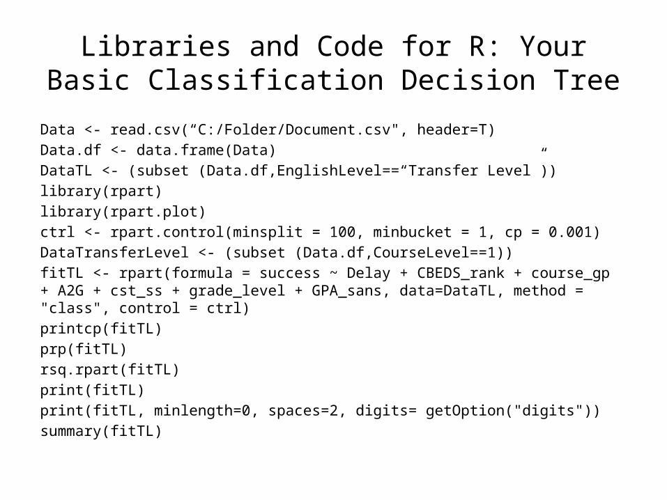
Libraries and Code for R: Your Basic Classification Decision Tree

Data <- read.csv(“C:/Folder/Document.csv", header=T)Data.df <- data.frame(Data)DataTL <- (subset (Data.df,EnglishLevel==“Transfer Level”))library(rpart)library(rpart.plot)ctrl <- rpart.control(minsplit = 100, minbucket = 1, cp = 0.001)DataTransferLevel <- (subset (Data.df,CourseLevel==1)) fitTL <- rpart(formula = success ~ Delay + CBEDS_rank + course_gp + A2G + cst_ss + grade_level + GPA_sans, data=DataTL, method = "class", control = ctrl)printcp(fitTL)prp(fitTL)rsq.rpart(fitTL)print(fitTL) print(fitTL, minlength=0, spaces=2, digits= getOption("digits"))summary(fitTL)

18

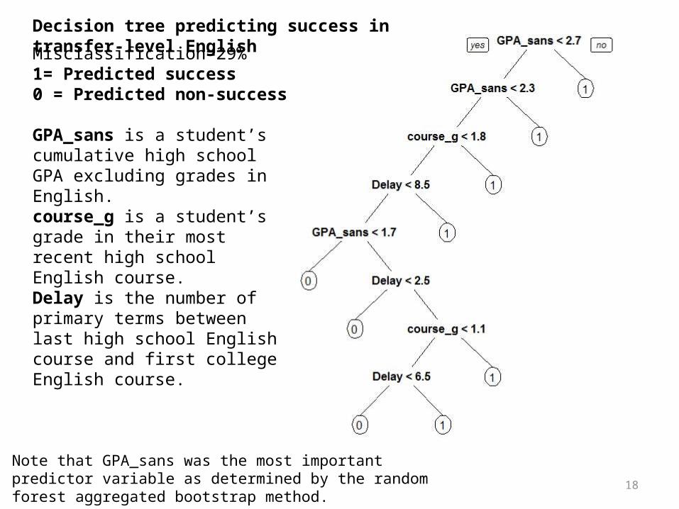
Misclassification=29%1= Predicted success0 = Predicted non-success

GPA_sans is a student’s cumulative high school GPA excluding grades in English.course_g is a student’s grade in their most recent high school English course.Delay is the number of primary terms between last high school English course and first college English course.

Decision tree predicting success in transfer-level English

Note that GPA_sans was the most important predictor variable as determined by the random forest aggregated bootstrap method.

19

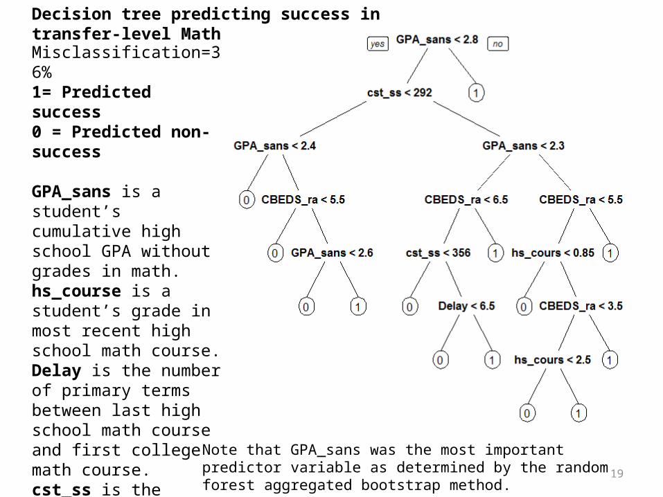
Decision tree predicting success in transfer-level Math

Misclassification=36% 1= Predicted success0 = Predicted non-success

GPA_sans is a student’s cumulative high school GPA without grades in math.hs_course is a student’s grade in most recent high school math course.Delay is the number of primary terms between last high school math course and first college math course.cst_ss is the scaled score from a student’s California Standards Test (CST).CBEDS_ra is the rank or level of a student’s last high school math course.

Note that GPA_sans was the most important predictor variable as determined by the random forest aggregated bootstrap method.

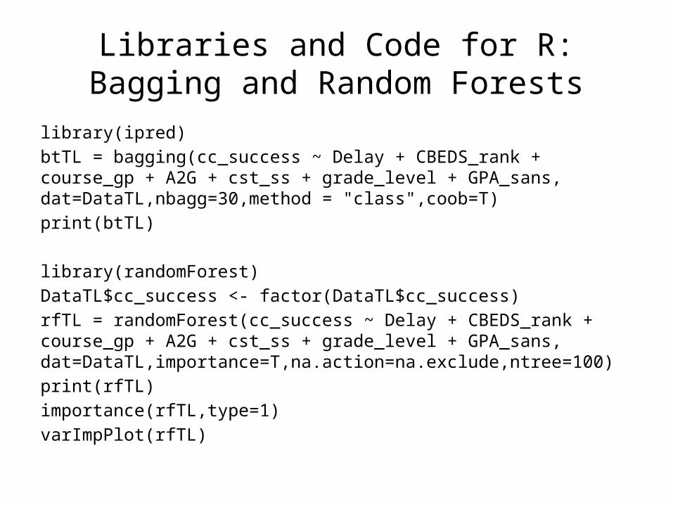
Libraries and Code for R: Bagging and Random Forests

library(ipred)btTL = bagging(cc_success ~ Delay + CBEDS_rank + course_gp + A2G + cst_ss + grade_level + GPA_sans, dat=DataTL,nbagg=30,method = "class",coob=T)print(btTL)

library(randomForest)DataTL$cc_success <- factor(DataTL$cc_success)rfTL = randomForest(cc_success ~ Delay + CBEDS_rank + course_gp + A2G + cst_ss + grade_level + GPA_sans, dat=DataTL,importance=T,na.action=na.exclude,ntree=100)print(rfTL)importance(rfTL,type=1)varImpPlot(rfTL)

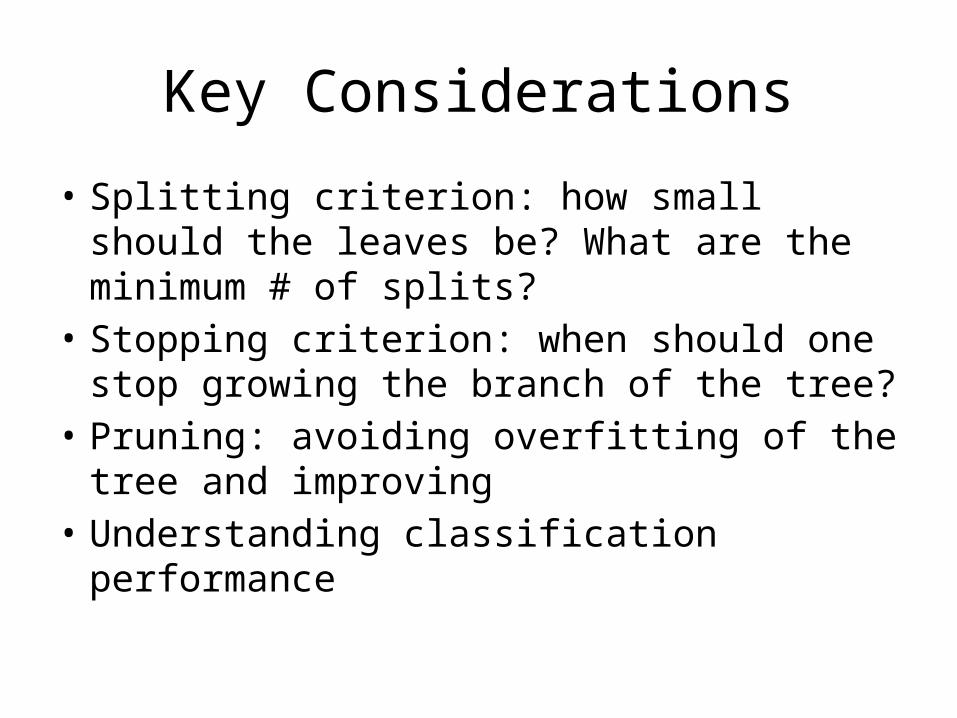
Key Considerations

• Splitting criterion: how small should the leaves be? What are the minimum # of splits?

• Stopping criterion: when should one stop growing the branch of the tree?

• Pruning: avoiding overfitting of the tree and improving

• Understanding classification performance

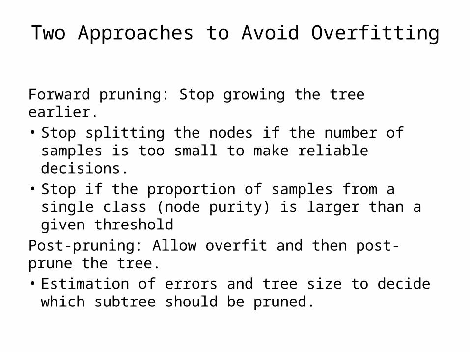
Two Approaches to Avoid Overfitting

Forward pruning: Stop growing the tree earlier.• Stop splitting the nodes if the number of samples

is too small to make reliable decisions.• Stop if the proportion of samples from a single

class (node purity) is larger than a given thresholdPost-pruning: Allow overfit and then post-prune the tree.• Estimation of errors and tree size to decide which

subtree should be pruned.

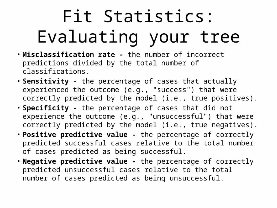
Fit Statistics: Evaluating your tree• Misclassification rate - the number of incorrect predictions divided by

the total number of classifications.• Sensitivity - the percentage of cases that actually experienced the

outcome (e.g., "success") that were correctly predicted by the model (i.e., true positives).

• Specificity - the percentage of cases that did not experience the outcome (e.g., "unsuccessful") that were correctly predicted by the model (i.e., true negatives).

• Positive predictive value - the percentage of correctly predicted successful cases relative to the total number of cases predicted as being successful.

• Negative predictive value - the percentage of correctly predicted unsuccessful cases relative to the total number of cases predicted as being unsuccessful.

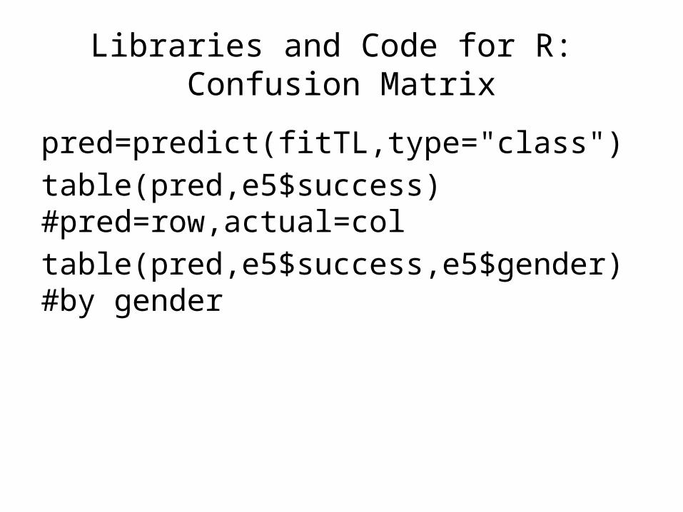
Libraries and Code for R: Confusion Matrix

pred=predict(fitTL,type="class")table(pred,e5$success) #pred=row,actual=coltable(pred,e5$success,e5$gender) #by gender

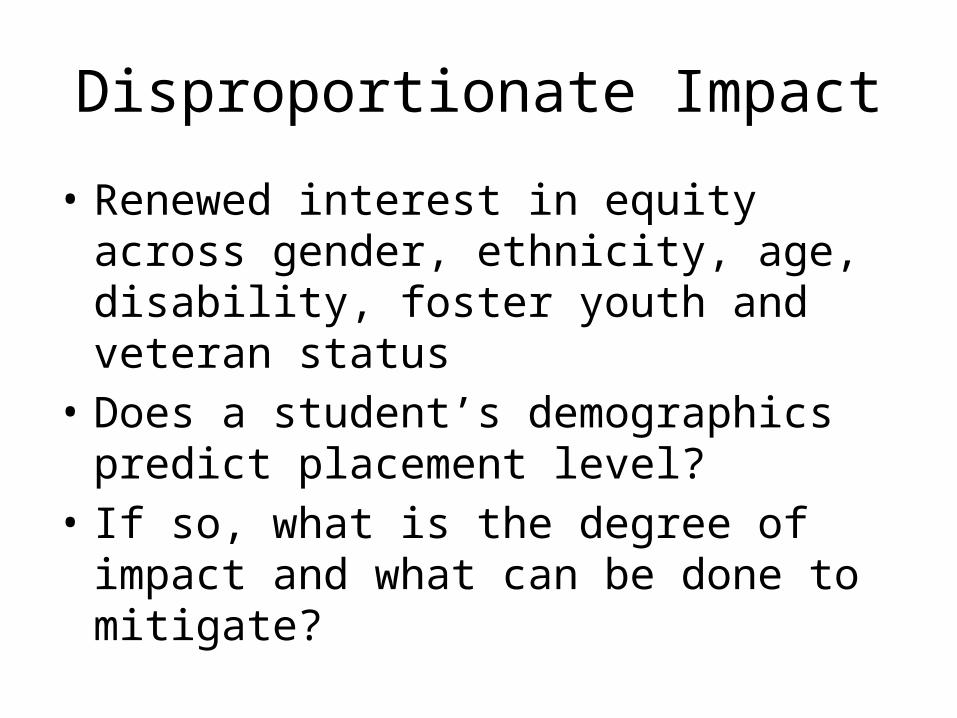
Disproportionate Impact

• Renewed interest in equity across gender, ethnicity, age, disability, foster youth and veteran status

• Does a student’s demographics predict placement level?

• If so, what is the degree of impact and what can be done to mitigate?

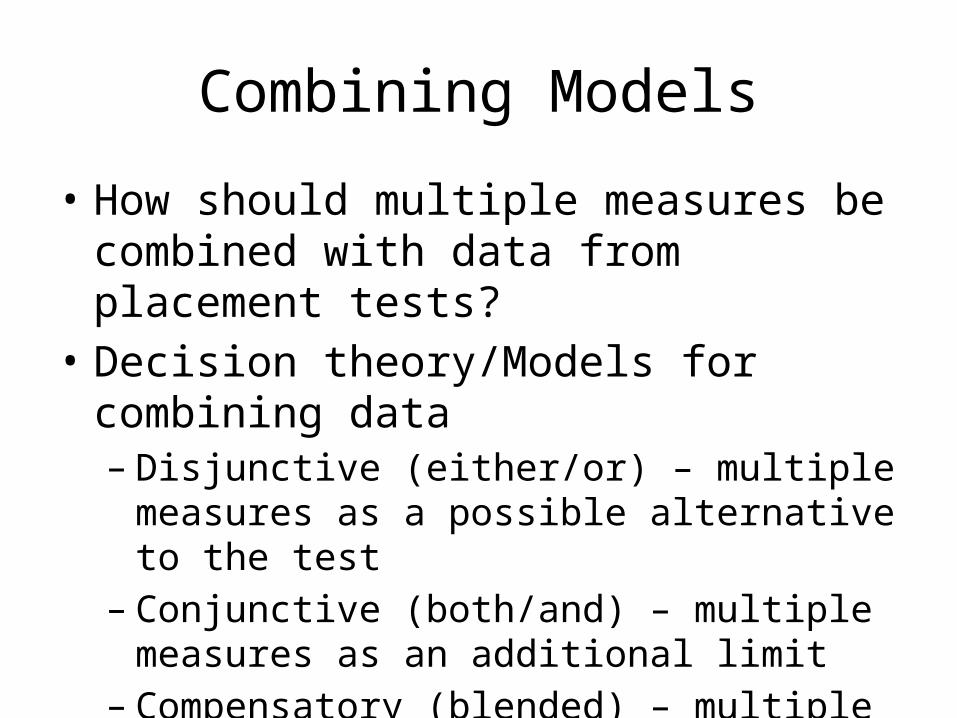
Combining Models

• How should multiple measures be combined with data from placement tests?

• Decision theory/Models for combining data– Disjunctive (either/or) – multiple measures as a

possible alternative to the test– Conjunctive (both/and) – multiple measures as an

additional limit– Compensatory (blended) – multiple measures as

an additional factor in an algorithm

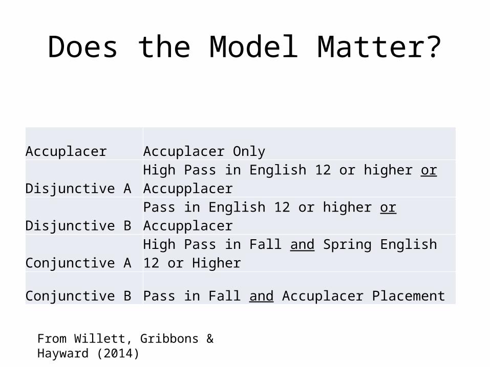
Does the Model Matter?

Accuplacer Accuplacer Only

Disjunctive A High Pass in English 12 or higher or Accupplacer

Disjunctive B Pass in English 12 or higher or Accupplacer

Conjunctive A High Pass in Fall and Spring English 12 or Higher

Conjunctive B Pass in Fall and Accuplacer Placement

From Willett, Gribbons & Hayward (2014)

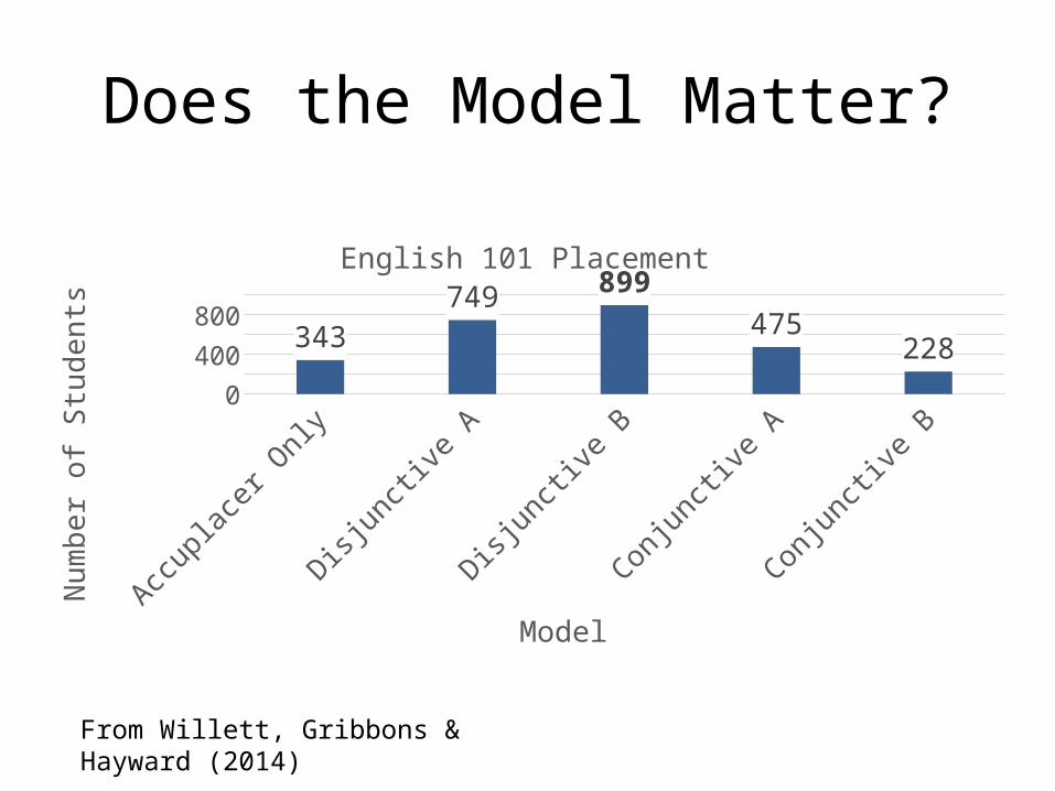
Does the Model Matter?

Accuplacer Only

Disjunctive A Disjunctive B Conjunctive A

Conjunctive B

0

200

400

600

800

1000

343

749899

475

228

English 101 Placement

Model

Num

ber o

f Stu

dent

s

From Willett, Gribbons & Hayward (2014)

Thank youCraig HaywardDirector of Planning, Research, and AccreditationIrvine Valley Collegechayward@ivc.edu

John HettsSenior Director of Data ScienceEducational Results Partnershipjhetts@edresults.org

Ken SoreyDirector, CalPASS Plusken@edresults.org

Terrence WillettDirector of Planning, Research, and Knowledge SystemsCabrillo Collegeterrence@cabrillo.edu