Embed Size (px)
Citation preview
MSc Stochastics and Financial Mathematics
Master Thesis
Using Artificial Neural Networks in theCalculation of Mortgage Prepayment
Risk
Author: Supervisor:Robben Riksen dr. P.J.C Spreij
Examination date: Daily supervisor:August 22, 2017 dr. B. Wemmenhove
dr. P.W. den Iseger
Korteweg-de Vries Institute forMathematics
ABN AMRO Bank N.V.

Abstract
A mortgage loan comes with the option to prepay (part of) the full amount of the loanbefore the end of the contract. This is called mortgage prepayment, and poses a risk tothe bank issuing the mortgage due to the loss of future interest payments. This thesisreviews some general properties of artificial neural networks, which are then applied topredict prepayment probabilities on mortgage loans. The Universal Approximation The-orem for neural networks with continuous activation functions will be treated extensively.Suggestions for a prepayment model based on neural networks are made.
Title: Using Artificial Neural Networks in the Calculation of Mortgage Prepayment RiskAuthor: Robben Riksen, [email protected], 10188258Supervisor: dr. P.J.C SpreijDaily supervisor: dr. B. Wemmenhove, dr. P.W. den IsegerSecond Examiner: dr. Asma KhedherExamination date: August 22, 2017
Korteweg-de Vries Institute for MathematicsUniversity of AmsterdamScience Park 105-107, 1098 XG Amsterdamhttp://kdvi.uva.nl
ABN AMRO Bank N.V.Gustav Mahlerlaan 101082 PP Amsterdamhttp://www.abnamro.com/
2

Contents
Introduction 5
List of Abbreviations 10
1. Mortgage Prepayment 111.1. An introduction to mortgages . . . . . . . . . . . . . . . . . . . . . . . . . 111.2. The current prepayment model . . . . . . . . . . . . . . . . . . . . . . . . 13
1.2.1. Explanatory variables . . . . . . . . . . . . . . . . . . . . . . . . . 141.2.2. Model description . . . . . . . . . . . . . . . . . . . . . . . . . . . 16
1.3. The underlying short-rate model . . . . . . . . . . . . . . . . . . . . . . . 171.3.1. The one-factor Hull-White model . . . . . . . . . . . . . . . . . . . 181.3.2. Fitting the model to the initial forward curve . . . . . . . . . . . . 201.3.3. The Nelson-Siegel-Svensson model . . . . . . . . . . . . . . . . . . 20
2. Artificial Neural Networks 232.1. Neural networks, an introduction . . . . . . . . . . . . . . . . . . . . . . . 232.2. Universality of neural networks . . . . . . . . . . . . . . . . . . . . . . . . 262.3. Optimization methods . . . . . . . . . . . . . . . . . . . . . . . . . . . . . 40
2.3.1. Cost functions . . . . . . . . . . . . . . . . . . . . . . . . . . . . . 402.3.2. Gradient descent . . . . . . . . . . . . . . . . . . . . . . . . . . . . 412.3.3. The Adam optimizer . . . . . . . . . . . . . . . . . . . . . . . . . . 42
2.4. Backpropagation . . . . . . . . . . . . . . . . . . . . . . . . . . . . . . . . 432.4.1. The backpropagation algorithm . . . . . . . . . . . . . . . . . . . . 432.4.2. Learning slowdown . . . . . . . . . . . . . . . . . . . . . . . . . . . 45
2.5. Activation and output functions . . . . . . . . . . . . . . . . . . . . . . . 452.5.1. Output functions . . . . . . . . . . . . . . . . . . . . . . . . . . . . 452.5.2. Activation functions . . . . . . . . . . . . . . . . . . . . . . . . . . 46
2.6. Weight initialization . . . . . . . . . . . . . . . . . . . . . . . . . . . . . . 492.6.1. ReLU initialization . . . . . . . . . . . . . . . . . . . . . . . . . . . 49
2.7. Reduction of overfitting . . . . . . . . . . . . . . . . . . . . . . . . . . . . 52
3. Simulations 553.1. Method . . . . . . . . . . . . . . . . . . . . . . . . . . . . . . . . . . . . . 55
3.1.1. Data collection . . . . . . . . . . . . . . . . . . . . . . . . . . . . . 553.1.2. Model selection . . . . . . . . . . . . . . . . . . . . . . . . . . . . . 583.1.3. Pricing the prepayment option . . . . . . . . . . . . . . . . . . . . 61
3.2. Results . . . . . . . . . . . . . . . . . . . . . . . . . . . . . . . . . . . . . . 62
3

4. Conclusion 68
5. Discussion and Further Research 695.1. Advantages and disadvantages of artificial neural networks . . . . . . . . . 695.2. Further research . . . . . . . . . . . . . . . . . . . . . . . . . . . . . . . . 715.3. Review of the process . . . . . . . . . . . . . . . . . . . . . . . . . . . . . 71
Popular summary 73
Bibliography 75
Appendices 78
A. Additional Theorems and Definitions 79A.1. Theorems for Chapter 1 . . . . . . . . . . . . . . . . . . . . . . . . . . . . 79A.2. Theorems for Chapter 2 . . . . . . . . . . . . . . . . . . . . . . . . . . . . 83
B. The Stone-Weierstass Theorem 86
C. Historical Proof of the Universal Approximation Theorem 90
4

Introduction
A mortgage is a special kind of loan issued by a bank or another mortgagor. It is used tofund the purchase of real estate by the client, with the purchased property as collateral.Since the property purchased with the mortgage loan can be sold if the client fails tomake his contractual payments, the conditions of a mortgage loan are often better thanthose of an ordinary client loan. The term mortgage is derived from the word ‘mortgaige’, death pledge, in old French. So called because the deal ends, or dies, either whenthe debt is paid or when payment fails. While in modern French the word is replaced by‘hypotheque’, the word mortgage was introduced in the English language in the MiddleAges and has been used since.When buying a house in the Netherlands, it is very common to take a mortgage on thatproperty. Over 81% of Dutch home owners and half of the Dutch households have amortgage1. With an average mortgage loan of around e267.000 and a summed totalof almost 81 billion euros for new mortgages in 20162, the dutch mortgage market wasworth a total of 665 billion euros in terms of outstanding loans in September 2016. Atthe end of 2016 ABN AMRO had a market share of 22% in this market3, making it veryimportant to quantify the risks that come with writing out a mortgage loan. A big partof this risk for the mortgagor lies in the possibility of default of the client, as becamepainfully clear during the 2008 financial crisis. However, there is another factor thatposes a risk. Clients have the possibility to pay back (a part of) the loan earlier thandiscussed in the contract. Since the mortgagor makes money of the loan by receivinginterest, this will decrease the profitability of the mortgage. Especially when taking intoaccount that clients are more likely to do this when the interest rates prevailing in themarket are lower than the contractual interest rate on the mortgage. Furthermore, theseso-called prepayments cause a funding gap in the sense that the prepaid money has to beinvested earlier than expected, often leading to less profitable investments when marketinterest rates are low.To calculate the prepayment risk and hedge against it, it is necessary to be able toestimate the prepayment ratio for certain groups of clients well. After arranging theclients in groups that show more or less similar behaviour, this is the fraction of clientsin that group that prepay their mortgage. A good estimation of the prepayment ratiowill reduce the costs that arise by over-hedging prepayment risk and is also requiredwhen reporting risks to the market authority (AFM). On top of this, the prepaymentrisk is used to calculate the fair price of penalties for the client that come with certainprepayment options.
1http://statline.cbs.nl2Kadaster3ABN AMRO Annual Report 2016
5
There are many reasons clients choose to make prepayments on their mortgage loan.When the interest rate for new mortgage contracts is lower than the contractual mortgageof a client, the client has a financial incentive to pay off his mortgage and get a new one,or to sell his house and buy a new house with a mortgage contract with a lower interestrate. But not many people will be tempted to move or renegotiate their mortgage everytime the interest rates are low. In economical terms, when not moving they are making‘irrational’ decision. Another example of economically irrational client behaviour ismoving when the interest rates are high, e.g. when in need of more space because of thebirth of a child.This thesis was written during an internship at ABN AMRO. The current model toestimate the prepayment ratio at ABN AMRO is based on a multinomial regression,taking into account many variables that can be of influence in prepayment decisions.This master thesis aims to find an alternative method to calculate the prepayment ratiousing artificial neural networks. Neural networks proved their worth in fields includingimage, pattern and speech recognition, classification problems, fraud detection and manymore. Loosely modelled after the brain, they are assumed to be good at tasks humans arebetter at than computers. Among other things, we therefore hope that neural networksare better at capturing the ‘irrational’ behaviour of clients than traditional methods.
Artificial neural networks
Before giving a brief introduction into feedforward artificial neural networks, we willshortly summarize the history and recent developments in this field.
History and current developments
Surprisingly, artificial neural networks first appeared even before the age of computers.In 1943 McCulloch and Pitts [24] introduced a model inspired by the working of thebrain that took binary inputs and produced binary outputs and regulated the firingof a neuron using a step function. By their ability to represent the logical AND andOR functions, it was possible to implement Boolean functions. In 1958 Rosenblatt [30]published an article about the perceptron, a simple model where input is processed in oneneuron with a step function and a learning algorithm that could be used in classificationproblems. Due to its simplicity it is still often used as an introduction to the theory ofartificial neural networks. However, it is incapable of implementing the logical exclusiveor (XOR) function, hence only able to solve linearly separable classification problems.This was seen as a huge drawback. Another drawback was that neural networks withmore neurons needed a lot of computational power to train well, which was simply notavailable at the time. Interest and funding in this field of research faded for a while,until the publication of a famous article in 1986 by Rumelhart, Hinton and Williams[33] popularizing the backpropagation algorithm (Section 2.4) which had already beenintroduced in the seventies, but had remained largely unnoticed. Backpropagation solvedthe exclusive or problem, allowing the fast training of bigger and deeper (i.e. more layers
6
of neurons) neural networks. This made the interest in artificial neural networks riseagain and a lot of progress was made. Nowadays, the increase of computational powerand the abundance of available data to train big neural networks, has led to manypromising results in many fields of application. Artificial neural networks are booming.The developments in this field of research are rapid. A lot of articles introducing state-of-the-art techniques are still in preprint, but the techniques might have already becomeindustry standard. It is an applied research area, so many methods are based solely onempirical results. When proofs do appear, they are often applied in situations wherenot all of the assumptions are satisfied. The argument ‘I don’t know why, but it works’always wins. This of course to great frustration of a mathematician. In this thesis wewill therefore spend some pages to show the theoretical capabilities of artificial neuralnetworks.
What are artificial neural networks?
As mentioned before, artificial neural networks are more or less modelled after the (hu-man) brain. The nodes in a neural network are therefore often called neurons. Similarto the neurons in the brain, artificial neurons generate output based on the input theyreceive. An artificial neural network consists of three types of neurons: input neurons,hidden neurons and output neurons. The most common type of artificial neural networkis the feedforward network. Information enters the network through the input neurons.The input neurons send the input to the first layer of hidden neurons. These hiddenneurons receive the inputs and apply a so-called activation function to an affine trans-formation of the inputs. That activation is then sent to the neurons in the next layer,where this process repeats itself. When the signal reaches the output layer, the outputneurons generate the output of the network by applying an output function to an affinetransformation of the received activations. To conclude, a neural network is a functiontaking input and generating output. The objective is to find the right function for acertain problem. It can be ‘trained’, optimized to generate the right output given itsinput, by choosing the parameters for the affine transformations made in every neuronin the network. A schematic representation of an artificial neural network is given inFigure 1.To train a network properly, large amounts of data are required. A neural networkwithout training does not know what function it has to approximate. Therefore, thetraining data has to consist of many input points with their required (although possiblynoisy) outputs. Training data is fed into the network, generating output. The output ofthe network is then compared to the desired output (the targets), to compute the error ofthe network. To change the parameters in a way that the error decreases, often a variantof the gradient descent algorithm is applied. All in all, this means that the exact formof the neural network is not pre-programmed, but it ‘learns’ how to deal with the data.After a lot of training, one hopes that the parameters at which the training algorithmarrives make the output of the neural network approximate the desired function wellenough.
7

Input 1
Input 2
Input 3
Input 4
Output
Hiddenlayer
Inputlayer
Outputlayer
Figure 1.: A neural network with four input nodes, a hidden layer with five hidden nodesand one output node.
Outline of the thesis
This thesis aims to explore the application of artificial neural networks in the estimationof prepayment risk on mortgages. It will both look at the theory of neural networks ingeneral and at the application to this specific problem.The first chapter will deal with mortgage prepayment. It will describe the specifics ofa dutch mortgage in Section 1.1, and explain the model that is currently used at ABNAMRO to predict mortgage prepayments in Section 1.2. Because the interest rate on amortgage is derived from swap rates, Section 1.3 is dedicated to describing the underlyingshort-rate model used in the simulations.Chapter 2 will cover the general theory of artificial neural networks, starting with thebasic definitions in Section 2.1. In Section 2.2, the theoretical value of neural networksis shown by two denseness results, often called the Universal Approximation Theorem.This section therefore has a more mathematical character than the other sections. Firstuniform denseness on compacta is shown in the set of continuous functions. Then, weshow denseness in the set of measurable functions with respect to the Ky Fan metric. Inthe remainder of Chapter 2 several options to optimize the performance and trainabilityof a network are discussed.In Chapter 3, simulations to estimate prepayment probabilities with a neural network aredescribed. We will describe how data was collected and how a final model was selected.Then in Section 3.2, the results of the simulations are given.In Chapter 4, a conclusion about the performance and usability of the selected modelwill be drawn from the simulation results. In Chapter 5, a discussion of the results andthe general usage of artificial neural networks will follow and some recommendationsfor further model improvements will be made. To conclude this chapter, we will brieflycomment on the process of this research.
8

Then, a popular summary of the subject is given. This summary should be accessibleto first year bachelor students in mathematics. In Appendix A, relevant theorems anddefinitions will be stated. For most of the theorems appearing here, the proof is omittedand the reader is referred to a source where the proof appears. In Appendix B, anelementary proof of the Stone-Weierstrass Theorem is given. The choice to state andprove this theorem in a separate appendix is made because the theorem and proof werenew to the author. The selected proof is surprising and uses only elementary propertiesof compact sets and continuous functions. Finally, Appendix C contains a historicallyrelevant proof of the Universal Approximation Theorem for a specific type of activationfunction.
9

List of Abbreviations
RIPU Remaining Interest Period Ultimo 14
HPI House Price Index (base year 2010) 14
LtV Loan to Value 15
ATM At-The-Money 18
NSS Nelson-Siegel-Svensson 20
ECB European Central Bank 20
MSE Mean Squared Error 40
CE Cross-Entropy 40
SGD Stochastic Gradient Descent 41
ReLU Rectified Linear Unit 46
LReLU Leaky Rectified Linear Unit 47
PReLU Parametric Rectified Linear Unit 47
ELU Exponential Linear Unit 47
FRA Forward Rate Agreement 80
10

1. Mortgage Prepayment
Before we can apply artificial neural networks to calculate the mortgage prepaymentrate, we first have to explain some properties of a dutch mortgage. To compare themodel using artificial neural networks with the current model, we will also describe asimplified version of the prepayment model as it is currently used at ABN AMRO. Inthe first section of this chapter, a short introduction to the general structure of dutchmortgages is given. In Section 1.2, the current mortgage prepayment model as usedat ABN AMRO is explained. Section 1.3 is dedicated to explaining the Hull-Whiteshort-rate model, which is necessary in our simulations to generate mortgage interestrates.
1.1. An introduction to mortgages
As defined in the Introduction, a mortgage is a loan issued by a bank or another mort-gagor that is used to fund the purchase of real estate by the client, with the purchasedproperty as collateral. The amount that the client borrows is called the principal ofthe loan. Whenever the borrower fails to pay off the loan, the mortgagor can sell theproperty in an attempt to reduce its losses and offset the loan (this is called foreclosure).Because of the size of the collateral, the size of a mortgage loan can be relatively highand interest rates for mortgages are relatively low compared to other types of loans.Usually the client pays monthly interest on the mortgage loan until the maturity (endof contract), at which the principal has to be fully repaid. The maturity of a mortgageis often 30 years. Different repayment schedules are discussed below. The interest rateon the mortgage can be variable or fixed. In the Netherlands in 2016, 52% of mortgageshave a fixed interest period between five and ten years, 20.5% of ten years or more,12.5% between one and five years and 15% up to one year or no fixed interest period1.Whenever the interest rate is fixed, it will remain the same during the agreed interestperiod. If the end of the interest period is before the maturity date of the contract, thebank and the client may agree on another interest period in which the interest rate willbe fixed again. When a fixed interest period ends and the client and the bank agree onnew conditions for a next interest period, we will view this as a total repayment of theloan and settlement of a new loan. Therefore, the maturity of a mortgage will be takenequal to the fixed interest period from now on. This is valid because the new conditionsmay differ significantly from the conditions on the old loan. Below we will summarizesome of the other characteristics of a mortgage loan.
1www.dnb.nl
11

Amortization schedule
When choosing a mortgage, a client can choose different amortization schedules, i.e.ways to repay the principal of the mortgage loan. The three amortization schedulesthat are currently offered at ABN AMRO are bullet (aflossingsvrij ), level paying (fixed-rate mortgage or annuıteitenhypotheek) and linear. In case of the bullet amortizationschedule, the client will only pay interest during the running time of the loan and repaythe full amount at the end of the contract. In a level paying loan, the client pays a fixedamount each month until the total amount of the loan has been repaid at the end ofthe contract. This implies that the monthly payments at the beginning of the contractmainly consist of interest and only by a small part of repayment, while towards the endof the contract the repayment size increases while the interest payments decrease. In thelinear schedule the client pays off a fixed amount of the loan each payment date. Theamortization schedules are schematically depicted in Figure 1.1 below.
Figure 1.1.: A schematic representation of the amortization schedules2. From left toright: bullet, level and linear.
Loan parts
A mortgage is often split into several loan parts that can have different conditions. Asituation in which this typically arises is when a client sells his house and decides to buya new house. The client now has to pay off his current mortgage and has to get a newone on the new house. The bank offers the option to get a mortgage on the new housewith the same conditions and outstanding principal as the old mortgage (meeneemoptie).However, if the new house is more expensive, the client will have a loan part with theconditions and of the size of the old mortgage and has to get another loan part with newconditions for the remaining amount to fund the house. Different loan parts can thereforehave different interest rates and different amortization schedules. In the following modelswe will therefore only look at loan parts, thus viewing every loan part as a full mortgageloan.
Prepayment options
Besides the different amortization schedules to repay the mortgage, the client has severalother options to repay (a part) of the loan before the contractual end date. This is called
2Adaptation of images fromhttps://www.abnamro.nl/nl/prive/hypotheken/hypotheekvormen/index.html
12

prepayment of the loan. Prepayment can be done in several ways. Some mortgages comewith a reconsider option. Clients with these mortgages have the option to renegotiatethe terms of their mortgage without extra costs during the reconsider period, usuallythe last two years of the fixed interest period. The prepayment categories as stated inthe ABN AMRO prepayment documentation [18] are
1. Refinancing: Full repayment of the loan without the collateral being sold, or anearly interest rate reset not taking place during an interest reconsider period.
2. Relocation: Full repayment of the loan in general caused by the sale of the collat-eral.
3. Reconsider (exercise of rentebedenktijdoptie): Full repayment of the loan withoutthe collateral being sold, or an early interest rate reset during an interest reconsiderperiod.
4. Curtailment high: Partial repayment of the loan, where the additional repaidamount is more than 10.5% of the original principal.
5. Curtailment low: Partial repayment of the loan, where the additional repaidamount is less than or equal to 10.5% of the original principal.
6. No event: Only contractual repayments.
As discussed in the Introduction, prepayment poses a risk for the bank. Therefore, ifthe prepayment is bigger than a certain percentage of the loan, called the franchise f , insome situations a penalty has to be payed. The franchise usually is 10% of the originalprincipal, although there are some mortgagors that maintain a franchise of 20%. Notethat in the categories above the franchise is set to 10.5%, to avoid the allocation ofcurtailment low to the event curtailment high due to data inaccuracies. Prepaymentsof the type relocation and reconsider are penalty free. The penalty therefore appliesto the prepayment classes curtailment high and refinancing. A situation where there isno penalty for any of the prepayment classes is when the mortgage interest rates in themarket are higher than the fixed mortgage rate in the contract.The calculation of the penalty assigned to each of the options is beyond the scope of thisthesis, but can be found in the ABN AMRO penalty model description [27].
1.2. The current prepayment model
Because the model used at ABN AMRO is confidential and because the main goal of thisthesis is the application of artificial neural networks, we will look at a simplified versionof the ABN AMRO multinomial prepayment model. For each type of prepayment,the model is used to predict the probability that a loan is prepayed in that way. Whengrouping similar loans together, these probabilities can then be interpreted as the fractionof the loans in a certain prepayment category.
13

In Subsection 1.2.1, the relevant explanatory variables that influence the prepaymentprobabilities will be introduced. In Subsection 1.2.2, a concise description of the multi-nomial regression model is given.
1.2.1. Explanatory variables
The traditional prepayment model is a multinomial regression model. It aims to predictthe prepayment fraction of a group of people with similar characteristics for each ofthe prepayment classes described in the last section. The model uses the followingcharacteristics of a mortgage loan as explanatory variables:
• Remaining interest period ultimo (RIPU): The number of months until the nextinterest reset date.
• Interest incentive: The incentive for prepayment caused by the mortgage interestrates.
• Loan age: The number of months from the start of the interest period up to thecurrent month.
• Penalty proxy: As a proxy for the penalty term, the interest incentive multipliedby the remaining interest period is taken.
• HPI ratio: The current House Price Index (HPI) divided by the HPI at the interestperiod start date.
• Amortization type: This can be bullet, level or linear.
• Interest term: The length of the interest period in months.
• Brand indicator: Can be ‘main brand’ or ‘non-main brand’.
• Seasonality: The current month.
• Personnel indicator: Indicates whether the client is ABN AMRO staff or not.
We will now shortly discuss each of the above mentioned explanatory variables. We willdescribe how it is used in the multinomial model and describe the possible influence ona prepayment event to justify its use as explanatory variable.
Remaining interest period ultimo
This is an important predictive variable since clients can only use the reconsider optionduring the last two years of the interest period. Furthermore, clients tend to relocatetowards the end of the interest period ([18]). As stated above, the RIPU is used in themodel as the number of months until the interest end date.
14

Interest incentive
This is one of the most important prepayment incentives. The interest incentive isdefined as the contractual interest rate minus the mortgage rate in the market for amortgage with the same fixed interest period. The bigger the interest incentive, themore interest costs for the client are reduced by prepayment. A big interest incentiveindicates low interest rates, also on saving accounts. If the interest rate received on asavings account is low, it is very beneficial to make small prepayments (curtailments)instead of putting money on the savings account.
Loan age
The older the loan, the higher the probability of refinance, since people will not do thisshortly after they signed the mortgage contract. Also there appears to be a peak inrelocations around 5 years after the start of the loan. On the other hand clients tend tocurtail if the loan age is small, since then the benefit is greatest.
Penalty proxy
Because the calculation of the penalty for certain prepayment events is quite involved,we will use a simplified penalty proxy. Since the costs for the bank are greatest when theremaining interest period is large and the interest incentive is big, the interest incentivemultiplied by the remaining interest period is used as a proxy. The penalty proxy istherefore an indication of how beneficial it is for the client to make a prepayment. Thus,a higher penalty proxy will increase the prepayment probabilities. This effect holds untilthe penalty becomes so large that the prepayment advantage is unmade.
HPI ratio
If the value of the house of a client increases, the loan-to-value ratio (LtV) of the mort-gage decreases. This makes it more attractive to refinance, since better terms might beagreed upon in a new contract. Also the probability of relocation will increase, becauseprofit will be made when the property is sold. Because the the mortgages are bundledinto buckets of loans with similar characteristics, it is impossible to recover the LtVratio for an individual loan. Instead, the HPI ratio is used as a proxy. A high HPI ratio(above 1) is an indication that the value of the house went up, a low HPI ratio indicatesa decrease in value. Curtailment appears to be more likely when the HPI ratio is wellabove 1, because those clients have more own funds to curtail with. On the other hand,if the HPI ratio is slightly below 1 clients will also curtail more to reduce the mortgageburden.
Amortization type
Different amortization types cause different curtailment behaviour. Clients with a levelamortization scheme curtail most in the beginning of the contract. There the benefit of
15

curtailment is greatest, since the contractual repayments are small. Linear mortgagescurtail least, because their contractual repayments start right after the signing of thecontract.
Interest term
Longer interest terms will cause a higher curtailment rate, because the benefits of cur-tailment in the beginning of the contract are bigger for a long maturity.
Brand indicator
If the mortgage is taken directly from ABN AMRO, then the brand indicator is ‘mainbrand’. If the contract is signed through an intermediary it is a ‘non-main brand’mortgage. Main brand mortgages tend to curtail and refinance less than non-mainbrand mortgages.
Seasonality
The month has a big effect on the prepayment rates and distinct seasonal effects areobserved. For example, refinancing and curtailment go up near the end of the year whenpeople review their mortgage and savings balance and curtailment can possibly cause atax benefit. Furthermore, there is a strong seasonality on the house market. Significantlymore houses are sold during the summer months. This will increase the relocation ratioin these months. Possible changes in regulations may drive up the relocation probabilitynear the end of the year as well.
Personnel indicator
A member of the ABN AMRO staff is more likely be aware of the reconsider option andtherefore the reconsider rate is higher for staff.
1.2.2. Model description
Consider a mortgage loan with a known vector X of explanatory variables as describedabove in Subsection 1.2.1. We want to calculate the probability that a certain prepay-ment is made. Let j denote the prepayment event as numbered in Section 1.1 (i.e. j = 1means refinancing etc.). We will write πj for the probability of a prepayment of categoryj. Traditionally, using no event as pivot in the multinomial regression, the probabilitieson events are estimated as
πj =eX·βj
1 +∑5
k=1 eX·βk
, for j = 1, . . . , 5,
and
π6 =1
1 +∑5
k=1 eX·βk
,
16

where βj is a vector of parameters specified in [18], usually different for each j. Ifan explanatory variable is not relevant for a prepayment category, the correspondingparameter entry in βj will be zero.However, to handle the reconsider prepayment category correctly, we need to adapt themethod slightly, since a reconsider prepayment can only be done in the reconsider period(conversely, refinancing can only take place outside the reconsider period, for otherwiseit would be a reconsider event). We therefore define
ηj = eX·βj , for j = 2, 4, 5,
and
η1 =
eX·β1 if not in reconsider period
0 if in reconsider period,
η3 =
0 if not in reconsider period
eX·β3 if in reconsider period.
The prepayment probabilities are then specified as
πj =ηj
1 +∑5
k=1 ηkfor j = 1, . . . , 5,
and
π6 =1
1 +∑5
k=1 ηk.
For a more detailed description of the ABN AMRO multinomial prepayment model andhow the parameter vectors βj are estimated, see [18].To evaluate the prepayment probabilities for a portfolio on different time instants in thefuture, a prediction of the mortgage rate in the market is needed to calculate the interestincentive. This is discussed in Section 1.3. For the HPI on future time points, the HPIforecast of ABN AMRO is used. The construction of this forecast is beyond the scopeof this thesis.
1.3. The underlying short-rate model
The market mortgage rate MT (t) at time t for a mortgage with maturity T is given bythe swap rate ST of a swap with maturity T plus a certain spread δT ,
MT (t) = ST (t) + δT . (1.1)
Since the goal of this thesis is to describe the prepayment model and investigate theuse of artificial neural networks in calculating the prepayment risk, we choose to usea simple model to calculate the short rates. Furthermore, it is convenient to choose a
17

model that has analytic expressions for the swap rates. This saves us the effort of havingto construct a trinomial tree (e.g. Appendix F in [3]) to make numerical calculations ofthe swap rates feasible. For this reason we will use the one-factor Hull-White model tocalculate short rate scenarios.During this section, we assume to be on a probability space (Ω,F ,P) with filtrationF = Ftt≥0 satisfying the usual conditions. We also assume there exists an equiva-lent martingale measure Q ∼ P. We will often refer to Appendix A, where necessarydefinitions and theorems are stated.
1.3.1. The one-factor Hull-White model
This subsection will give a recap of the one-factor Hull-White model [15], in order toderive an analytic expression for the swap rates ST (t) in terms of the initial instantaneousforward curve, the zero-coupon bond prices at t = 0 and the short rate. The short ratedynamics under Q are
dr(t) = (b(t) + β(t)r(t)) dt+ σ(t) dW ∗t ,
where W ∗t is a Q-Brownian motion, β(t), σ(t) are chosen to obtain the desired volatilitystructure and b(t) is chosen to match the current initial forward curve. In this thesis,we will use a slightly simplified version of this model, where we take β and σ constant:
dr(t) = (b(t) + βr(t)) dt+ σ dW ∗t . (1.2)
To find an analytic expression for the ATM swap rates (see Appendix A.1, equation(A.5)), we need to find the T -bond prices. Recall the definition of a model with an affineterm-structure from [9].
Definition 1.1. A short-rate model provides an affine term-structure if there are smoothfunctions A and B such that
P (t, T ) = e−A(t,T )−B(t,T )r(t). (1.3)
Note that in this definition, for fixed T , P is a function of t ∈ [0, T ] and r(t). Tofind a characterization of short-rate models with an affine term structure, we apply theFeynman-Kac formula (Theorem A.1) to the right hand side of equation (1.3). Thisleads to Corollary A.2 in Appendix A.1.Now clearly the one-factor Hull-White model satisfies the form of equation (A.8) witha(t) = σ, α(t) = 0 and β(t) = β. Using these to solve the differential equations (A.9)and (A.10) will show that this model has an affine term-structure. For B(t, T ) we seethat equation (A.10) becomes
∂tB(t, T ) = −βB(t, T )− 1, B(T, T ) = 0,
which we can solve straightforwardly to find
B(t, T ) =1
β
(eβ(T−t) − 1
).
18

Integrating equation (A.9) for A yields
A(t, T ) = −σ2
2
∫ T
tB2(s, T ) ds+
∫ T
tb(s)B(s, T ) ds. (1.4)
To solve this equation further, we first need to find a more explicit expression for b(t).For the first part we follow the line of reasoning of [9]. Using the affine term structureand the definition of the instantaneous forward rate (equation (A.4)), we can write
f(0, T ) = ∂TA(0, T ) + ∂TB(0, T )r(0).
Using Leibniz integral rule and the fact that ∂TB(t, T ) = −∂tB(t, T ) we write
f(0, T ) =σ2
2
∫ T
0∂sB
2(s, T ) ds+
∫ T
0b(s)∂TB(s, T ) ds+ eβT r(0)
= − σ2
2β2
(eβT − 1
)2+
∫ T
0b(s)eβ(T−s) ds+ eβT .
If we now define the function
φ(T ) :=
∫ T
0b(s)eβ(T−s) ds+ eβT ,
we find that φ(T ) = f(0, T ) + σ2
2β2
(eβT − 1
)2and, again by Leibniz integral rule, that
∂Tφ(T ) = βφ(T ) + b(T ). Solving this for the function b gives us
b(t) = ∂tφ(t)− βφ(t)
= ∂t
(f(0, t) +
σ2
2β2
(eβt − 1
)2)− βf(0, t)− σ2
2β
(eβt − 1
)2= ∂tf(0, t)− βf(0, t)− σ2
2β
(1− e2βt
). (1.5)
Having found this expression for b we can now integrate in equation (1.4) to find A(t, T ).Using that B(T, T ) = 0, partial integration and (A.4), we get after a lot of calculus
A(t, T ) = −σ2
2
∫ T
tB2(s, T ) ds+
∫ T
tb(s)B(s, T ) ds
=
∫ T
tf(0, s) ds− f(0, t)B(t, T )− σ2
4β
(1− e2βt
)B(t, T )2
= − log
(P (0, T )
P (0, t)
)− f(0, t)B(t, T )− σ2
4β
(1− e2βt
)B(t, T )2.
Hence, given the initial instantaneous forward curve and the zero-coupon bond pricesat t = 0, we can by virtue of the affine term structure calculate the zero-coupon bondprices at all t ≤ T and therefore the swap rates.
19
1.3.2. Fitting the model to the initial forward curve
In Subsection 1.3.1, we derived an expression for the function b to match the current termstructure (equation (1.5)). However, the expression involved a derivative of the initialforward curve which can be inconvenient and increases the effect of a possible observationerror. To get rid of the derivative, we will introduce a different representation of theone-factor Hull-White model, which is described in [3]. Solving the stochastic differentialequation for the short rate and substituting the found expression for b gives
r(t) = r(0)eβt +
∫ t
0eβ(t−s)b(s) ds+
∫ t
0σeβ(t−s) dW ∗s
= f(0, t) +σ2
2β2
(1− eβt
)2+
∫ t
0σeβ(t−s) dW ∗s
= α(t) +
∫ t
0σeβ(t−s) dW ∗s ,
where we defined the function
α(t) := f(0, t) +σ2
2β2
(1− eβt
)2.
Hence it is clear that r(t) is normally distributed with mean α(t) and variance equal to∫ t0 σ
2e2β(t−s) ds = σ2
2β
(e2βt − 1
).
To find a convenient way to simulate these short rate paths, we will define a process xby the dynamics
dx(t) = βx(t)dt+ σdW ∗t , x(0) = 0.
This implies that
x(t) = σ
∫ t
0eβ(t−s) dW ∗s ,
sor(t) = α(t) + x(t).
The short rate now consists of a deterministic part α(t) reflecting the initial term-structure and a stochastic process x(t), independent of the initial market conditions,which we can simulate.
1.3.3. The Nelson-Siegel-Svensson model
Using the results from subsections 1.3.1 and 1.3.2, we can generate swap rates and shortrate sample paths, given the initial instantaneous forward rate curve. Therefore, weneed a model that fits the observed market data well. This is a field of research by itself,but since we only need one model, we will confine ourselves to a short description of the
20

Nelson-Siegel-Svensson model (NSS). This model is currently used by the ECB and theparameters for the current market structure are quoted daily on their website.The precursor of the NSS model was introduced by Nelson and Siegel ([25]) and gave aparametrization of the spot rate in four parameters
R(0, T ) = β0 + β11− e−T/τ
T/τ+ β2
(1− e−T/τ
T/τ− e−T/τ
).
They argue that β0 captures the long term structure, β1 is the contribution of the shortterm effects and β2 is the medium-term component that can cause the typical hump-shape in the curve.Svensson later added a term and two extra parameters to improve the fit with a secondhump-shape ([36]). The spot rate model becomes
R(0, T ) = β0 + β11− e−T/τ1T/τ1
+ β2
(1− e−T/τ1T/τ1
− e−T/τ1)
+ β3
(1− e−T/τ2T/τ2
− e−T/τ2).
Recalling the definitions of the spot rate and instantaneous forward rate, equations (A.3)and (A.4) respectively, we see that
f(0, T ) = R(0, T ) + T∂
∂TR(0, T ),
so in the NSS model we find a forward rate of
f(0, T ) = β0 + β1e−T/τ1 + β2
T
τ1e−T/τ1 + β3
T
τ2e−T/τ2 .
In Figure 1.2 the different components of the forward rate are plotted separately toillustrate their effect on the forward rate curve.Using the ECB parameters for the Nelson-Siegel-Svensson model, we now have all theingredients to generate swap rates with initial conditions matching the current marketstructure.
21

Figure 1.2.: Two examples of the Nelson-Siegel-Svensson forward rate (uninterruptedline) and all components plotted separately. The parameters used in theupper plot are from the ECB for 1 December 2016, the parameters in thelower plot are from 11 December 2007.
22

2. Artificial Neural Networks
In this chapter we will introduce the concept of artificial neural networks. We will lookat feedforward networks and prove that even the functions produced by neural networkswith only one hidden layer are uniformly dense on compacta in C(R). This shows thatwe can indeed use artificial neural networks to approximate any continuous function.We will also show density in the set of measurable functions with respect to the Ky Fanmetric. After this, we will discuss the choice of different cost and activation functionsfor the network to increase performance and introduce the backpropagation algorithmto update the network after each training cycle. The last section of this chapter willdescribe methods to reduce overfitting.Throughout this chapter we will denote by L the number of layers of a network and bydl the number of neurons in layer l. This means that d0 denotes the dimension of theinput and dL the dimension of the output (and targets).
2.1. Neural networks, an introduction
In this section we will use a modified version of the notation used by Bishop [2] andNielsen [26]. A neural network is used to approximate an often unknown and complicatedfunction f : Rd0 → RdL , (x1, . . . , xd0) 7→ (t1, . . . , tdL). Thus, the goal is to create a neuralnetwork that takes an input vector x = (x1, . . . , xd0) and produces an output vectory = (y1, . . . , ydL) that is a good approximation of the target vector t = (t1, . . . , tdL). Aneural network consists of layers of neurons (also called nodes or units) that each receivea certain input and generate an output. A neuron takes an affine transformation of theinput it receives, the result is called the weighted input of the neuron. The output of theneuron is called the activation and is obtained by applying an activation function to theweighted input. The activation function can be chosen depending on the application ofthe network. Historically, so-called sigmoidal functions (non-decreasing functions fromR to [0, 1] approaching 0 in the negative and 1 in the positive limit, Definition C.3) werethe most commonly used activation functions. An example of a sigmoidal function isthe logit function. For this reason, we denote the activation function in this section byσ. Nowadays, sigmoidal functions are often replaced by other activation functions. Fora discussion about different types of activation functions, see Section 2.5.A neural network consists of layers: one input layer, a number of hidden layers and oneoutput layer. Figure 2.1 gives a schematic representation of a neural network.The hidden layers are called like this because they only interact with neurons inside thenetwork. In this sense they are ‘hidden’ from the outside of the network. Consider anetwork with L layers. By convention we do not count the input layer, so there are
23

Hiddenlayer 1
Hiddenlayer 2
Inputlayer
Outputlayer
Figure 2.1.: A neural network with three input nodes, two hidden layers with five hiddennodes each and two output nodes.
L−1 hidden layers and 1 output layer. The input layer is built up out of so called inputneurons. These are special in the sense that they take only one input and do not havean activation function. Input neuron i takes input xi and sends the same xi as outputto all neurons in the first hidden layer. Therefore the number of input neurons is equalto the dimension d0 of the input. Let’s say the first hidden layer consists of d1 neurons.Each hidden neuron in this layer receives input from all the input neurons and takesan affine transformation of these to produce its weighted input. The weighted input ofhidden neuron j in hidden layer 1 is therefore
z(1)j =
d0∑i=1
w(1)ji xi + b
(1)j ,
where constants w(1)ji are called the weights of hidden neuron j for input i and the
constant b(1)j is called the bias of hidden neuron j. Note that there are d1 nodes in the
first hidden layer, so there are d1 × d0 weights and d1 biases necessary to compute allweighted inputs of this layer. We can represent the d1-dimensional vector of the weightedinputs of the first hidden layer as a matrix vector multiplication
z(1) = W (1)x + b(1),
where W (1) is the weight matrix with entries w(1)ji and x and b(1) are d0- and d1-
dimensional vectors of the inputs and biases respectively. The activation of a hiddenneuron is defined as the activation function σ applied to the weighted input of the neuron.For neuron j in the first hidden layer, the activation therefore is
a(1)j = σ(z
(1)j ).
24

After the calculation of the activations in the first hidden layer, the process is repeatedas the information flows to the next hidden layer. The output of one layer is the inputfor the next layer. In general we therefore find that the activation of neuron j in layer lis given by
a(l)j = σ(z
(l)j ) = σ
dl−1∑i=1
w(l)ji a
(l−1)i + b
(l)j
.
Equivalently, the activation vector of layer l is given by
a(l) = σ(W (l)a(l−1) + b(l)),
where the activation function σ is applied component-wise. After passing through thehidden layers, the signal goes to the output layer, consisting of dL output neurons. Theyagain take a weighted sum and add a bias. So for j = 1, . . . , dL the output neuronsweighted input is
z(L)j =
dL−1∑i=1
w(L)ji a
(L−1)i + b
(L)j ,
where w(L)ji is the weight of output neuron j for hidden neuron i and b
(L)j is the bias
for output neuron j. The output vector of the network is the activation function of theoutput layer, denoted by h, applied to its weighted input. The output of the neuralnetwork is therefore given by the vector with components
yj = h(z(L)j ), j = 1, . . . , dL,
or in vector notation
y = h(z(L)) = h(W (L)a(L−1) + b(L)
).
Note that the output y of the network is a function of the input x and the weights andbiases of the network. The choice of the output activation function h depends on theapplication, see Section 2.5, but for regression problems often a linear output activationfunction h(x) = x is chosen.We thus see that a neural network takes affine transformations of the inputs, appliesan activation function and repeats this process for each layer. Because the informa-tion moves in one direction – from the first to the last layer – networks of this kindare called feedforward networks. With a random choice of the weights and biases, theprobability of getting an output vector y close to the target vector t is of course minus-cule. Therefore, after initializing the weights and biases (for a discussion about differentweight initialization methods see Section 2.6) they need to be updated and improved toget more accurate output vectors. This is done by choosing a suitable cost function tomeasure the approximation error (Subsection 2.3.1) and minimizing the cost function byupdating the weights according to an optimization method (Section 2.3).
25

To train and judge the performance of a network, a lot of data is needed. The datasetshould consist of many d0-dimensional input vectors and corresponding dL-dimensionaltarget values. This is why training these types of networks is called supervised learning :a set of input values is needed for which we already know the (maybe noisy) outputvalues of the function we want to approximate. Often the available data is split into atraining set, a validation set and a test set to reduce the risk of overfitting (see Section2.7). The training data is used to optimize the weights and biases in the network. Thevalidation data is then used to choose suitable meta-parameters, i.e. parameters otherthan the weights and biases, like the number of layers. Finally the performance of thenetwork is tested on the test data. There is a lot to say about the choices to be madewhen designing a neural network. But before we delve into neural networks any deeper,we want to know what functions artificial neural networks are able to approximate.
2.2. Universality of neural networks
In this section we will show that even shallow neural networks, i.e. networks with onlyone hidden layer, with linear output neurons are able to approximate any Borel measur-able function with arbitrary precision if sufficiently many hidden neurons are available.Historically, this result, often called the ‘Universal Approximation Theorem’, was shownin 1989 by Hornik, Stinchcombe and White [14], see Appendix C, and separately byCybenko [7]. This first version of the Universal Approximation Theorem only works forneural networks with sigmoidal activation functions, see Definition C.3.The theorem by Hornik et al. sufficed for a long time, when neural networks were mainlyused with sigmoidal activation functions, like the standard logit function. However, cur-rently the most used activation function is the Rectified Linear Unit (f(x) = max0, x,see Subsection 2.5.2). This activation function is unbounded and therefore does notsatisfy the definition of a sigmoidal function. Luckily, it is possible to prove a UniversalApproximation result for activation functions that are continuous but not polynomial.The proof was originally done by Leshno et al. [20], but we will loosely follow the lineof the proof in a review article by Pinkus [28].In both articles, the proof only applies to one-layer neural networks and shows densenessin the topology of uniform convergence on compacta in C(Rn), the class of continuousfunctions from Rn to R. However, using some lemmas from [14], we can expand theresult to multi-layer networks and to denseness in Mn, the set of measurable functionsfrom Rn to R. The main results of this section are Corollary 2.11, stating that one-layerneural networks are uniformly dense on compacta in C(Rn) and Corollary 2.24, statinga similar denseness result for multi-layer multi-output neural networks. It also showsdenseness with respect to a different metric in Mn,m, the class of measurable functionsfrom Rn to Rm.In this section we will use notation that is conventional in literature, where σ denotesthe (possibly not sigmoidal) activation function. We define the class of functions thatcan be the output of a one-layer neural network with input x ∈ Rn and one linear outputneuron.
26

Definition 2.1. For any Borel measurable function σ : R→ R and n ∈ N we define theclass of functions
Σn(σ) : = span g : Rn → R | g(x) = σ(w · x + b); w ∈ Rn, b ∈ R
=
f : Rn → R | f(x) =
d∑i=1
biσ(Ai(x)); bi ∈ R, Ai ∈ An, d ∈ N
,
where An is defined as the set of all affine functions from Rn to R.
A polynomial is the finite sum of monomials. By the degree of a polynomial we meanthe maximum degree of its monomials, which is the sum of the powers of the variablesin the monomial. Before we start with proving the main result of this section, wewill shortly mention a converse statement. Suppose that the activation function σ is apolynomial, say of degree d. Then clearly Σn(σ) is the space of polynomials of degreed. This directly implies that Σn(σ) cannot be dense in C(Rn). Thus, if we want tofind activation functions for which Σn(σ) is dense in C(Rn), we do not have to look atpolynomials.Next, we will specify what we mean by uniform denseness on compacta.
Definition 2.2. A subset S ⊂ C(Rn) is called uniformly dense on compacta in C(Rn) iffor every compact subset K ⊂ Rn, for every ε > 0 and for every f ∈ C(Rn) there existsa g ∈ S such that supx∈K |f(x)− g(x)| < ε.
The main theorem of this section is based on an older result concerning ridge functions.These are defined as follows.
Definition 2.3. A function f : Rn → R is called a ridge function if it is of the formf(x) = g(a · x), for some function g : R→ R and a ∈ Rn \ 0.
In fact, note that the activation of a neuron in a single layer neural network, σ(w ·x+b),is a ridge function for every activation function σ, every w and b.The necessary theorem, when making our way to Corollary 2.11, is a result by Vostrecovand Kreines [38] from 1961. However, we follow the line of the proof to the theoremfrom [21] and [29].Recall that homogeneous polynomials are polynomials for which each term has the samedegree. Let us denote the linear space of homogeneous polynomials of n variables ofdegree k by Hn
k . Note that the dimension of Hnk is
(n+k−1
k
).
Theorem 2.4. Let A be a subset of Rn. The span of all ridge functions
R(A) := spanf : Rn → R | f(x) = g(a · x); g ∈ C(R), a ∈ A
is uniformly dense on compacta in C(Rn) if and only if the only homogeneous polynomialthat vanishes on A is the zero polynomial.
27
Proof. Given any direction a ∈ A, we note that R(A) also contains g(λa · x) for allλ ∈ R, since R(A) allows all functions g in C(R), so we can absorb λ in the function.This means that we are done by proving the result for sets A ⊆ Sn−1, the unit spherein Rn.‘ =⇒ ’: We will prove this by contradiction. Assume that R(A) is dense in C(Rn) andthere exists a nontrivial homogeneous polynomial p of some degree k that vanishes onA.By assumption, p is of the form
p(x) =d∑j=1
cjxmj,1
1 · · ·xmj,nn =
d∑j=1
cjxmj ,
for some d ∈ N, coefficients cj and mj,i ∈ Z+ such that∑n
i=1mj,i = k for all j. Wealso denoted by mj the vector (mj,1, . . . ,mj,n) ∈ Zn+ and introduced the useful notationxm = xm1
1 · · ·xmnn .
Now pick any φ ∈ C∞c (Rn), the set of infinitely dimensional functions from Rn to Rwith compact support, such that φ is not the zero function. For notational convenience,define for m ∈ Zn+ with
∑imi = k the operator
Dm =∂k
∂xm11 · · · ∂x
mnn
.
Then, define the function ψ as
ψ(x) :=
d∑j=1
cjDmjφ(x).
Note that ψ ∈ C∞c (Rn) and also ψ 6= 0. Using repeated partial integration and the factthat φ has compact support, we see that the Fourier transform of ψ becomes
ψ(x) =1
(2π)n/2
∫Rn
e−iy·xψ(y) dy
=1
(2π)n/2
d∑j=1
cj
∫Rn
e−iy·xDmjφ(y) dy
=ik
(2π)n/2
d∑j=1
cjxmj,1
1 · · ·xmj,nn
∫Rn
e−iy·xφ(y) dy
= ikφ(x)p(x). (2.1)
Because of the homogeneity of p, we find that p(λa) = λkp(a) = 0 for all a ∈ A. Byequation (2.1), this also implies that ψ(λa) = 0 for all a ∈ A. For such an a, we find
0 = ψ(λa) =1
(2π)n/2
∫Rn
ψ(y)e−iλa·y dy
=1
(2π)n/2
∫ ∞−∞
∫a·y=t
ψ(y) dy e−iλt dt.
28
Since the equality holds for all λ ∈ R, it follows that∫a·x=t
ψ(x) dx = 0, ∀t ∈ R.
Hence, for all g ∈ C(R) and a ∈ A,∫Rn
g(a · x)ψ(x) dx =
∫ ∞−∞
(∫a·x=t
ψ(x) dx
)g(t) dt = 0.
Thus, the positive linear functional defined by
F (f) :=
∫Rn
f(x)ψ(x) dx,
for f ∈ C∞c (Rn), annihilates R(A).Let K ⊂ Rn be compact such that K contains the support of ψ. On C(K) we can nowapply the Riesz-Markov-Kakutani Representation Theorem (Theorem A.3 in Appendix)to find that there exists a unique Borel measure µ on K such that
F (f) =
∫Kf(x) dµ(x),
for all f ∈ Cc(K). By the denseness of R(A) in C(K), we must have that µ is the zeromeasure on K, making F an operator mapping everything to zero. This however is acontradiction, since F (ψ) > 0. Because this holds for any k ∈ N, we conclude that thereexists no nontrivial homogeneous polynomial p that vanishes on A.‘ ⇐= ’: Select any k ∈ Z+. By assumption no nontrivial homogeneous polynomial ofdegree k is identically zero on A.For any a ∈ A, define
g(a · x) := (a · x)k =N∑j=1
(k
mj,1, . . . ,mj,n
)amjxmj =
N∑j=1
k!
mj,1! · · ·mj,n!amjxmj ,
where N =(n+k−1
k
). Then g(a · x) is in both R(A) and Hn
k .The linear space Hn
k has dimension N and a basis consisting of xmj , for mj such that∑ni=1mj,i = k and j = 1, . . . , N . Therefore, its dual space (Hn
k )′ has a basis of functionalsfj , j = 1, . . . , N , for which fj(x
mi) = δji, where δ is the Kronecker delta. See e.g. [34],Theorem A.4 in the Appendix for this result.Now note that
Dmjxmi = δjimj,1! · · ·mj,n!.
Hence, for a linear functional T on Hnk , there exists a polynomial q ∈ Hn
k such that
T (p) = q(D)p, for each p ∈ Hnk . Also, for any q ∈ Hn
k , we see q(x) =∑N
j=1 bjxmj , for
29
some coefficients bj ∈ R, j = 1, . . . , N . So
q(D)g(a · x) =
N∑j=1
bjDmj
(N∑i=1
k!
mi,1! · · ·mi,n!amixmi
)
= k!N∑j=1
bjamj
= k! q(a).
Thus, if the linear operator T annihilates g(a · x) for all a ∈ A, then its representingpolynomial q ∈ Hn
k vanishes on A. By assumption, this means that q is the zero polyno-mial, hence T maps every element in Hn
k to zero. This shows that no nontrivial linearfunctional working on Hn
k can map g(a · x) to zero for all a ∈ A. Therefore we see that
Hnk = spanf : Rn → R | f(x) = g(a · x); a ∈ A ⊆ R(A).
Since this holds for any k ∈ Z+, we note thatR(A) contains all homogeneous polynomialsof any degree, and therefore all polynomials. The Weierstrass Approximation Theorem,or the more general Stone-Weierstrass Theorem (Theorem B.3 in Appendix B), nowyields that R(A) is uniformly dense on compacta in C(Rn).
To give an example of a set A to which we can apply Theorem 2.4, note that if Acontains an open subset of Sn−1 (in the relative topology), then the only homogeneouspolynomial vanishing on A is the zero polynomial.For a subset Λ ⊂ R and a subset A ⊆ Sn−1, we denote the set λa | λ ∈ Λ,a ∈ Aby Λ ∧ A. Then, to reduce the dimension of our problem, we have the following simpleproposition.
Proposition 2.5. Assume Λ,Θ ⊆ R such that
N (σ; Λ,Θ) := spang : R→ R | g(x) = σ(λx+ b); λ ∈ Λ, b ∈ Θ
is uniformly dense on compacta in C(R). Furthermore, assume that A ⊆ Sn−1 is suchthat R(A) is uniformly dense on compacta in C(Rn). Then
Σn(σ; Λ ∧A,Θ) := spang : Rn → R | g(x) = σ(w · x + b); w ∈ Λ ∧A, b ∈ Θ
is uniformly dense on compacta in C(Rn).
Proof. Let f ∈ C(Rn) and K ⊆ Rn be compact. Let ε > 0. By denseness on compactaof R(A) in C(Rn), there exists a d ∈ N, functions gi ∈ C(R) and ai ∈ A for i = 1, . . . , dfor which
|f(x)−d∑i=1
gi(ai · x)| < ε
2, ∀x ∈ K.
30

Now, because K is compact, and therefore bounded, there exist finite (compact) intervals[αi, βi], for i = 1, . . . , d, such that ai·x | x ∈ K ⊆ [αi, βi]. Furthermore, by the assumeddenseness of N (σ; Λ,Θ) in C([αi, βi]), for i = 1, . . . , d, we can find constants cij ∈ R,λij ∈ Λ and bij ∈ Θ, for j = 1, . . . ,mi and some mi ∈ N, such that
|gi(x)−mi∑j=1
cijσ(λijx+ bij)| <ε
2d,
for all x ∈ [αi, βi] and i = 1, . . . , d. Hence, by the triangle inequality,
|f(x)−d∑i=1
mi∑j=1
cijσ(λijai · x + bij)| < ε, ∀x ∈ K.
This shows the result.
Now, being allowed to do the work on R, we will show a density result for activation func-tions in C∞(R), the set of infinitely differentiable functions. We first need an adaptationof a lemma from [8].
Lemma 2.6. Let f be in C∞(R) such that for every point x ∈ R there exists a kx ∈ Nfor which f (kx)(x) = 0. Then f(x) is a polynomial.
Proof. DefineG as the open set of all points for which there exists an open neighbourhoodon which f(x) equals a polynomial. In other words, G is the set of points for which thereexists an open neighbourhood on which f (k)(x) = 0 for some k (and hence for all k′ > kas well). Define the closed set F := Gc. We assume F is not empty and work towards acontradiction.First note that F cannot have isolated points. To see this, suppose x0 is an isolatedpoint of F . Then there are a, b ∈ R such that (a, x0) ⊂ G and (x0, b) ⊂ G. On (a, x0), fcoincides with a polynomial which can be found by the Taylor expansion of f around x0.The same holds for the polynomial f coincides with on the interval (x0, b). Together,this means that f coincides with this polynomial on the whole interval (a, b), showingthat x0 cannot be in F .We will next define the closed sets En as the subsets of F on which f (n) vanishesidentically. Note that F = ∪nEn, by the assumed property of the derivatives of f .Clearly, being a closed subset of a complete metric space, F is complete as well and wecan apply the Baire Category Theorem (Theorem A.6 in Appendix A). This theoremstates that F cannot be the countable union of nowhere dense sets, implying that theinterior of EN in F must be nonempty for some N . In other words, it contains anopen ball in F : an x0 ∈ F , such that for ε > 0 small enough, all points y ∈ F withd(x0, y) < ε are also in En. Now take I to be a closed interval around x0, small enoughto have F ∩ I ⊆ EN . Then clearly F (N)(x) = 0 for all x ∈ F ∩ I. Because F does nothave isolated points and f (N)(x)−f (N)(y) = 0 for all x, y ∈ F ∩ I, it follows that f (N+1)
also vanishes identically on F ∩ I. Repeating the argument show that f (m)(x) = 0 forall m ≥ N and x ∈ F ∩ I.
31

Furthermore, we realize that F ∩ I cannot contain an interval, since that interval wouldthen belong to G. Hence, G ∩ I is not empty. Because G is open and I is an interval,there must be a (small) interval (a, b) in G ∩ I with endpoints a, b ∈ F ∩ I. By thenature of G, f is equal to a polynomial on (a, b), hence, as before, this polynomialcan be obtained from its Taylor expansion around either of the endpoints. Since allderivatives f (k)(a) = f (k)(b) = 0 for all k ≥ N , we see that f (N)(x) = 0 on the wholeof (a, b). Since this holds for any arbitrary interval in G ∩ I and also on F ∩ I, we canconclude that f (k)(x) = 0 on all of I for all k ≥ N . This contradicts x0 ∈ F , since wehave shown that at least the interior of I is in G. We conclude that F = ∅, thus f is apolynomial.
The proof of the following proposition uses the converse of the lemma. For now we takeΛ = Θ = R. Denote by P the set of all polynomials.
Proposition 2.7. Let σ ∈ C∞(R) and σ /∈ P. Then N (σ;R,R) is dense in C(R)uniformly on compacta.
Proof. By the converse of Lemma 2.6, there exists a point b0 such that σ(k)(b0) 6= 0 forall k ∈ N.Calculating the derivative of σ(λx+ b0) in λ = 0, we find
d
dλσ(λx+ b0)
∣∣∣∣λ=0
= limh→0
σ((λ+ h)x+ b0)− σ(λx+ b0)
h
∣∣∣∣λ=0
= xσ′(b0). (2.2)
So xσ′(b0) ∈ N (σ;R,R), since it is the limit of elements in N (σ;R,R). Similarly
dk
dλkσ(λx+ b0)
∣∣∣∣λ=0
= xkσ(k)(b0), (2.3)
and xkσ(k)(b0) ∈ N (σ;R,R) for all k ∈ N. Because σ(k)(b0) 6= 0 for all k ∈ N, wehave shown that N (σ;R,R) contains all the monomials of all degrees and therefore allpolynomials. Let K ⊆ R compact. Then from the Weierstrass Approximation Theoremit follows that N(σ;R,R) is dense in C(K).
We can easily combine the above results into the following Corollary.
Corollary 2.8. Let σ ∈ C∞(R) and σ /∈ P. Then Σn(σ) is uniformly dense on compactain C(Rn).
Proof. By Proposition 2.7, it follows that N (σ;R,R) is uniformly dense on compacta inC(R). Taking A equal to the unit sphere Sn−1, R(A) is uniformly dense on compacta inC(Rn) by Theorem 2.4. Now, by Proposition 2.5 we conclude that Σn(σ;Rn,R) is densein C(Rn), uniformly on compacta.
When working with C∞ activation functions to approximate continuous functions, thisresult is sufficient. But we can even take our weights and biases from a smaller set thanR and still have the uniform approximation result. Looking at the proof of Proposition
32

2.7, for Lemma 2.6 to hold, we only need Θ to be an open interval on which σ is nota polynomial. Further on in the proof, we see that the only constraint on Λ is that wecan evaluate equations (2.2) and (2.3). We can therefore give a more general corollaryto the result.
Corollary 2.9. Let Λ,Θ ⊆ R be such that Λ contains a sequence tending to zero andΘ is an open interval. Furthermore let A ⊆ Sn−1 such that A contains an open set inthe relative topology and take σ ∈ C∞(Θ) such that σ is no polynomial on Θ. ThenN (σ; Λ,Θ) is dense in C(R) and Σn(σ; Λ ∧ A,Θ) is dense in C(Rn), both uniformly oncompacta.
We will now generalize the result of Proposition 2.7 to continuous activation functions.
Proposition 2.10. Let σ ∈ C(R) and σ /∈ P. Then N (σ;R,R) is dense in C(R)uniformly on compacta.
Proof. For any φ ∈ C∞c (R), the class of infinitely differentiable functions with compactsupport, define
σφ(x) := σ ∗ φ(x) =
∫ ∞−∞
σ(x− y)φ(y) dy,
the convolution of σ and φ. Because φ has compact support and σ and φ are continuous,σφ is well-defined for every t (the integral converges everywhere) and σφ ∈ C∞(R). If
we view the integral as a limit of Riemann sums, we see that σφ ∈ N (σ; 1,R). Since
σφ(λx+ b) =
∫ ∞−∞
σ(λx+ b− y)φ(y) dy,
we then have N (σφ;R,R) ⊆ N (σ;R,R). As in the proof of Proposition 2.7, we find that
xkσ(k)φ (b) ∈ N (σφ;R,R) for every b ∈ R and all k ∈ N.
We will finish the proof by contradiction. Suppose N (σ;R,R) is not dense in C(R).Then, it must be that xk /∈ N (σ;R,R) for some k. This implies that xk /∈ N (σφ;R,R),
hence σ(k)φ (b) = 0 for all b ∈ R. By Lemma 2.6 it now follows that σφ must be a
polynomial. Because its k’th derivative is identically zero, we also see that the degree ofσφ is at most k − 1. Note that the above holds for any φ ∈ C∞c (R).The next step is to find a sequence of φn ∈ C∞c (R) such that σφn → σ uniformlyon compacta. Taking the φn to be mollifiers, see Definition A.7 and Theorem A.9 inAppendix A.2, the desired convergence holds. Since all σφn are polynomials of degree atmost k − 1 and the space of polynomials of a certain degree is a closed linear space, weconclude that σ must also be a polynomial of degree at most k − 1. This contradictionshows the result.
We are now ready to state the equivalent of Corollary 2.8 for σ ∈ C(R), the main resultof this section. The proof is very similar, only with σ ∈ C(R) and Proposition 2.10instead of Proposition 2.7, and is therefore omitted.
33

Corollary 2.11. Let σ ∈ C(R) and σ /∈ P. Then Σn(σ) is uniformly dense on compactain C(Rn).
This already is an important result showing the capabilities of artificial neural networks,and in many cases this is enough. However, we can even show that neural networks aredense in some way inMn, the set of measurable functions from Rn to R. To prove this,we will first have to define the right metric on Mn.
Definition 2.12 (Ky Fan metric). Let µ be a probability measure on (Rn,B(Rn)).We define the metric ρµ on Mn by
ρµ(f, g) = infε > 0 : µ(|f − g| > ε) < ε.
From the definition of this metric, we see that two functions are close when the probabil-ity that they differ significantly is small. The relevance of this metric in approximationwith neural networks is when we take µ as the probability of occurrence of certain inputs.If a neural network is close to the target function f with respect to ρµ, it can only differsignificantly from f on input sets that occur with small probability.In Lemma 2.13 we show that convergence with respect to ρµ is equivalent to convergencein probability. We will formulate and prove three lemmas on the properties of this newlydefined metric.
Lemma 2.13. Let µ be a probability measure on (Rn,B(Rn)). For f, f1, f2, . . . ∈ Mn,the following statements are equivalent.
(i) ρµ(fm, f)→ 0.
(ii) For every ε > 0 we have µ(|fm − f | > ε)→ 0 (convergence in probability).
(iii)∫
min|fm(x)− f(x)|, 1 dµ(x)→ 0.
Proof. (i) =⇒ (ii): Take ε > 0. Want to show that µ(|fm − f | > ε) → 0. So letε′ > 0. Now by (i) we see that for n big enough µ(|fn − f | > ε) < ε. So assume ε′ < ε(otherwise we are done). In this case, again by (i) we can find a large m such thatµ(|fm − f | > ε) < µ(|fm − f | > ε′) < ε′.(ii) =⇒ (i): Let ε > 0. By (ii) we now that there exists a N such that m > Nimplies µ(|fm − f | > ε) < ε. But this immediately implies that ρµ(fm, f) = infε > 0 :µ(|fm − f | > ε) < ε ≤ ε for all m > N .(ii) =⇒ (iii): Let ε > 0. By virtue of (ii) there exists an N such that m > N impliesµ(|fm − f | > ε/2) < ε/2. Hence∫
min|fm(x)− f(x)|, 1 dµ(x) ≤ µ(|fm − f | > ε/2) + ε/2 < ε.
(iii) =⇒ (ii): Fix ε > 0. We see that∫min|fm(x)− f(x)|, 1 dµ(x) = µ(|fm − f | > 1) +
∫|fm(x)− f(x)|1|fm−f |≤1 dµ(x).
34
Since both terms are positive, by (iii) both go to 0 as m→∞. For the second term, wenote that∫
|fm(x)− f(x)|1|fm−f |≤1 dµ(x) ≥∫|fm(x)− f(x)|1ε<|fm−f |≤1 dµ(x)
≥ εµ(ε < |fm − f | ≤ 1),
thus µ(ε < |fm − f | ≤ 1)→ 0. Then, as m→∞,
µ(|fm − f | > ε) = µ(|fm − f | > 1) + µ(ε < |fm − f | ≤ 1)→ 0.
The next lemma, Lemma 2.14, relates uniform convergence on compacta to ρµ conver-gence.
Lemma 2.14. Let µ be a probability measure on (Rn,B(Rn)). Let f, f1, f2, . . . ∈ Mn.If fm → f uniformly on compacta, then ρµ(fm, f)→ 0.
Proof. We will show that (iii) from Lemma 2.13 holds. This then implies ρµ convergence.Let ε > 0. Because µ is a probability measure on a complete separable metric space, itis tight and we can take a closed and bounded (hence compact) ball K big enough suchthat µ(K) > 1 − ε/2. Since fm → f uniformly on compacta, we can find an N suchthat m ≥ N implies supx∈K |fm(x)− f(x)| < ε/2. Combining these we find that for allm ≥ N ∫
min|fm(x)− f(x)|, 1 dµ(x) =
∫1K min|fm(x)− f(x)|, 1 dµ(x)
+
∫1Kc min|fm(x)− f(x)|, 1dµ(x)
<ε
2+ε
2= ε.
Before we can state and prove the third lemma on the metric ρµ, we need to prove alemma on the denseness of C(Rn) in the set of integrable functions. Therefore, we needto introduce the concept of a regular measure.
Definition 2.15. Let (X,T ) be a topological space with F = σ(T ) a σ-algebra on X.Let µ be a measure on (X,F). A measurable subset A of X is called inner regular if
µ(A) = supµ(F ) | F ⊆ A,F closed
and outer regular ifµ(A) = infµ(G) | G ⊇ A,G open.
A measure is called inner regular (outer regular) if every measurable set is inner regular(outer regular). If a measure is both outer regular and inner regular, it is called a regularmeasure.
35

We will call a measure defined on all Borel sets a Borel measure. We will now show thatevery finite Borel measure is regular.
Proposition 2.16. Let X be a metric space endowed with the Borel σ-algebra. A finiteBorel measure µ on X is regular.
Proof. Define S as the collection of measurable regular sets A, i.e. the sets for which
µ(A) = infµ(G)|G ⊇ A,G open= supµ(F )|F ⊆ A,F closed.
We will show that S contains the Borel σ-algebra, which proves the proposition.Firstly, note that S contains all measurable open sets. Clearly for A open, we haveµ(A) ≥ infµ(G) | G ⊇ A open since A itself is open. Also µ(A) ≤ infµ(G) : G ⊇A open since for every G ⊇ A it holds that µ(G) ≥ µ(A). Furthermore, since in ametric space every open set is a countable union of closed sets, we can conclude thatA ∈ S. We will finish the proof by showing that S is a σ-algebra.Clearly ∅ ∈ S. Take A ∈ S and let ε > 0. Since A ∈ S we can find sets F ⊆ A ⊆ G withF closed, G open and µ(A) < µ(F ) + ε, µ(A) > µ(G)− ε. Then Gc ⊆ Ac ⊆ F c and Gc
closed, F c open. Also
µ(Ac) = µ(X)− µ(A) > µ(X)− µ(F )− ε = µ(F c)− ε,
and
µ(Ac) = µ(X)− µ(A) < µ(X)− µ(G) + ε = µ(Gc) + ε.
This shows Ac ∈ S.Now let A1, A2, . . . ∈ S. We want to show that the countable union of these sets is againin S. Let ε > 0. For n ∈ N choose Gn ⊇ An open, such that µ(Gn \ An) < ε/2n. Then∪∞n=1Gn is open and µ (∪∞n=1Gn \ ∪∞n=1An) ≤ µ (∪∞n=1Gn \An) < ε.Since µ is finite, there exists an N such that µ (∪∞n=1An) − µ
(∪Nn=1An
)< ε/2. We can
also find Fn ⊆ An closed for n = 1, . . . , N such that µ(An \ Fn) < ε2N . Now ∪Nn=1Fn is
closed and contained in ∪∞n=1An. Furthermore
µ (∪∞n=1An)− µ(∪Nn=1Fn
)= µ (∪∞n=1An)− µ
(∪Nn=1An
)+ µ
(∪Nn=1An
)− µ
(∪Nn=1Fn
)<ε
2+ µ
(∪Nn=1An \ Fn
)<ε
2+N
ε
2N= ε.
This shows S is a σ-algebra containing the open sets, hence B ⊆ S. We conclude that µis a regular measure.
Using this result we can prove the lemma on the denseness of C(X) in the set of integrablefunctions.
36

Lemma 2.17. Let (X, d) be a metric space endowed with the Borel σ-algebra andlet µ be a finite Borel measure on X. Then C(X) is dense in L1(X,µ), the space of(equivalence classes of) integrable functions on X.
Proof. Let A ∈ B(X). Since µ is a finite measure on a metric space, by Proposition2.16 µ is regular. Therefore, we can find sequences of open sets Gn ⊇ A and closed setsFn ⊆ A such that µ(A \ Fn)→ 0 and µ(Gn \A)→ 0 as n→∞.For any nonempty closed C ⊂ X we will define the (continuous) function dC on Xmeasuring the distance to C by dC(x) := infy∈C d(x, y). Next define
fn(x) :=dGc
n(x)
dGcn(x) + dFn(x)
.
Then fn is continuous so fn ∈ C(X) and fn : X → [0, 1], such that fn = 0 on the closedset Gcn and fn = 1 on Fn. Hence 1Fn ≤ fn ≤ 1Gn . But this implies that fn → 1A in L1
by virtue of the squeeze lemma. This can be done for any A ∈ B(X).Now we have shown that we are able to approximate the indicator of any measurableset, we see that the indicator functions lie in C(X). By linearity this means that alsothe simple functions are in C(X). Since we can approximate functions in L1(X,µ) bysimple functions, we can conclude that L1(X,µ) is also contained in C(X) with respectto the L1 norm.
We will use the above result to show the third lemma on the ρµ-metric.
Lemma 2.18. For any probability measure µ on Rn, C(Rn) is dense in Mn, the set ofmeasurable functions from Rn to R, with respect to the ρµ-metric.
Proof. Let f ∈ Mn and let ε > 0. By the finiteness of the measure µ, we can find alarge M such that µ(|f | > M) < ε/2. But this implies that∫
min|f1|f |<M − f |, 1 dµ =
∫1|f |>Mmin|f |, 1dµ < µ(|f | > M) <
ε
2.
Using Lemma 2.17, we can find a function g ∈ C(Rn) such that∫|f1|f |<M − g| dµ < ε/2.
Application of the triangle inequality now yields∫min|g − f |, 1 dµ ≤
∫min|g − f1|f |<M|+ |f1|f |<M − f |, 1dµ
≤∫
min|g − f1|f |<M|, 1 dµ+
∫min|f1|f |<M − f |, 1 dµ
<ε
2+ε
2= ε.
By Lemma 2.13 we can now conclude that C(Rn) is dense inMn with respect to ρµ.
37

Finally we are ready to prove the denseness of Σn(σ) in Mn. Fortunately, we havealready done most of the work.
Corollary 2.19. Let µ be a probability measure on (Rn,B(Rn)) and let σ ∈ C(R) suchthat σ /∈ P. Then Σn(σ) is dense in Mn with respect to the metric ρµ.
Proof. By Theorem 2.11, Σn(σ) is uniformly dense on compacta in C(Rn). By Lemma2.14, this means that Σn(σ) is also dense in C(Rn) with respect to the ρµ-metric. In thesame metric, C(Rn) is dense inMn, by Lemma 2.18. By the triangle inequality we maynow conclude that Σn(σ) is dense in Mn with respect to ρµ.
In the following corollary, we will extend the result of Corollaries 2.11 and 2.19 to multi-output networks.
Definition 2.20. For any activation function σ ∈ C(R) such that σ /∈ P and n,m ∈ Nwe define the class of functions
Σn,m(σ) :=
f : Rn → Rm | f(x) =
d∑i=1
biσ(Ai(x)); bi ∈ Rm, Ai ∈ An, d ∈ N
.
Denote by Mn,m the class of measurable functions from Rn to Rm. We also need toexpand the definition of the ρµ to define a metric on Mn,m.
Definition 2.21. Let µ be a probability measure on (Rn,B(Rn)). We define the metricρmµ on Mn,m by
ρmµ (f, g) =
m∑i=1
ρµ(fi, gi),
where fi, gi denote the entries of f respectively g and ρµ is the metric onMn as definedin Definition 2.12.
The approximation result for for a one-layer neural network with m linear output neuronsnow follows easily.
Corollary 2.22. Let µ be a probability measure on (Rn,B(Rn)) and let σ ∈ C(R) suchthat σ /∈ P. Then Σn,m(σ) is uniformly dense on compacta in C(Rn,Rm) and dense inMn,m with respect to the metric ρmµ .
Proof. Let f ∈ C(Rn,Rm) and ε > 0. We will reduce the dimension of the prob-lem by approximating the vector elements of f separately. By Corollary 2.11 we canapproximate elements fj for each j ∈ 1, . . . ,m uniformly on compacta. So take acompact K ⊂ Rn. For j = 1, . . . ,m we can find functions gj ∈ Σn(σ) such that we have
supx∈K |gj(x) − fj(x)| < ε/m. By replacing the weights b(j)i in each of the approxima-
tions gj by vectors in Rm with zero entries except in the j’th position (where we put
b(j)i ) we get functions g′j in Σn,m(σ). Defining g =
∑mj=1 g
′j , we see g ∈ Σn,m(σ) and by
the triangle inequality the uniform difference on K is smaller than ε. Since we can do
38

this for every compact K ⊂ Rn, we conclude Σn,m(σ) is uniformly dense on compactain C(Rn,Rm)Exactly the same argument, but with f ∈ Mn,m, using Corollary 2.19 and the metricρµ, will yield the denseness result in Mn,m.
We now want to move to neural networks with L layers (note again that we do notcount the input layer, but do count the output layer). We will denote this class of neuralnetworks by Σn,m
L (σ).Before we can state the result on these networks, we need a lemma.
Lemma 2.23. Let F be a class of functions from R to R that is uniformly dense oncompacta in C(R) and G be a class of functions from Rn to R that is uniformly denseon compacta in C(Rn). The class H := f g : f ∈ F , g ∈ G is also uniformly dense oncompacta in C(Rn).
Proof. Let z ∈ C(Rn), let K ⊂ Rn be compact and ε > 0. Since G is dense on compactain C(Rn), we can find a g ∈ G such that supx∈K |g(x) − z(x)| < ε/2. Since z is acontinuous function, its image of K, z(x) : x ∈ K, is compact, hence closed andbounded. Now because g is uniformly close to z on K, we see that g(x) : x ∈ K isalso bounded.Define GK := g(x) : x ∈ K. GK is closed and bounded, thus compact. Therefore, wecan find an f ∈ F such that supx∈GK
|f(x)− x| < ε/2. But this implies that
supx∈K|f(g(x))− z(x)| ≤ sup
x∈K|f(g(x))− g(x)|+ sup
x∈K|g(x)− z(x)|
= supx∈GK
|f(x)− x|+ supx∈K|g(x)− z(x)|
< ε/2 + ε/2 = ε.
We conclude f g ∈ H approximates z uniformly on K. The result follows.
This last corollary will prove that multi-layer, multi-output neural networks with linearoutput neurons are also uniform approximators.
Corollary 2.24. Let µ be a probability measure on (Rn,B(Rn)) and let σ ∈ C(R) suchthat σ /∈ P. For every L ∈ N with L ≥ 2, Σn,m
L (σ) is uniformly dense on compacta inC(Rn,Rm) and dense in Mn,m with respect to the metric ρmµ .
Proof. Assume m = 1. Since the activation of one layer in the network is the input of thenext layer, we will proceed by induction to the number of layers. Suppose the number oflayers L = 2 (one hidden layer). In Corollary 2.11 we have already shown that Σn,1
2 (σ)is uniformly dense on compacta in C(Rn). This shows the induction hypothesis.Next suppose that Σn,1
L (σ) is uniformly dense in compacta in C(Rn). A network with
L+ 1 layers will just be a Σ1,11 (σ) function with as input the output of a Σn,1
L network.
By Corollary 2.11, Σ1,11 (σ) is uniformly dense on compacta in C(R). Hence application
of Lemma 2.23 yields that the L + 1 layer network, Σn,1L+1(σ), is uniformly dense on
compacta. This concludes the induction.
39
Repetition of the proof of Corollary 2.19 yields the result of denseness in Mn,1 withrespect to the ρµ-metric. To extend the result tom > 1, apply exactly the same techniqueas in Corollary 2.22.
These powerful results show that artificial neural networks with any number of hiddenlayers are in theory capable of approximating any measurable function from Rn to Rm,for any n,m ∈ N, with any desired precision. That is, if the activation function iscontinuous and not polynomial.With a strengthened trust in artificial neural networks, we can proceed with the discus-sion started in Section 2.1.
2.3. Optimization methods
In this section we will discuss several iterative optimization methods that may find theoptimal values for the weights and biases given the input and target values. Before wecan optimize the parameters, we have to define with respect to what metric we wantto minimize the difference between the targets t and network outputs y. The first sub-section will therefore introduce the cost function and give two examples of commonlyused cost functions. Training of neural networks is mainly done with gradient descentoptimization algorithms. Methods that involve the calculation of second-order deriva-tives, such as Newton’s methods, are often computationally not feasible due to the largenumber of parameters in a neural network. In Subsection 2.3.2, a short introductionto gradient descent optimization algorithms is given and in Subsection 2.3.3 the Adamoptimization algorithm is explained.
2.3.1. Cost functions
To measure how well the output of a neural network approximates the target values in thetraining stage, we need to define a cost (or error) function. These cost functions are oftenthe mean of the individual loss functions per training data point. Consider a trainingdata set X = x1, . . . ,xN with N data points and T = t1, . . . , tN the correspondingtargets (note that each data point and target is a d0- respectively dL-dimensional vector).Given these inputs and targets, the cost function becomes a function of the weights andbiases of the network
C(w,b | X , T ) =1
N
N∑n=1
Cn(w,b | xn, tn), (2.4)
where Cn(w,b) is loss function of the n’th input. A commonly used cost function inregression problems is the mean squared error (MSE) in which the loss functions takethe form Cn(w,b | x, t) = 1
2‖y − t‖2, where by ‖ · ‖ we denote the Euclidean norm andy = y(w,b | x) is the output of the neural network.In classification problems, where each sample can be in one class, the mean squarederror may not be the best cost function to use. A loss function that is often used in
40
classification problems is the cross-entropy (CE) error. For example, in [35] simulationsshow that using the cross-entropy error outperforms the mean squared error in classi-fication problems and even leads to faster training an improved generalization. This isalso in accordance our own observations while doing the simulations in Chapter 3. Thecross-entropy loss function is defined as
Cn(w,b | x, t) = −dL∑i=1
ti log(yi),
where y1, . . . , ydL and t1, . . . , tdL are the elements of the output vector y and the targetvector t and represent a probability distribution.
2.3.2. Gradient descent
One of the most well-know optimization algorithms is the iterative method known asgradient descent. For this we need a differentiable cost function and a starting pointof the algorithm. Each iteration is a step in the direction opposite to the gradient. Inthe case of neural networks, the weights and biases are set to their initial values andthe input vectors are fed through the network to generate the output vectors. Theseare then compared to the target values t by applying the cost function. As mentionedabove, given the input and the target values for that input, the cost function C is in facta function of the weights w and biases b of the network (since those fully determine theoutput). To find a minimum of the cost function, the weights and biases are changed inthe direction of steepest descent
w→ w − η∇wC, b→ b− η∇bC,
where η is the step size, called the learning rate. When the learning rate is too big, thereis a possibility of overshooting the minimum. On the other hand a too small learningrate will result in slow convergence.A straight-forward application of this optimization method is called batch gradient de-scent. Output is generated for all training samples and gradient descent is applied usingthe average cost of all the data. This means that we only update the weights and biasesonce, after evaluating the network on all of the training data. This might be too com-putationally intensive when dealing with larger datasets, resulting in very slow learning.The training data is therefore often split into so-called mini-batches of smaller size. Theweights and biases are then updated according to the gradient on a mini-batch. Bychoosing the mini-batches large enough, the gradient on this subset of the training datawill be approximately the same as the gradient of the full training data. Therefore, theweights and biases will be updated roughly in the same direction, but only the samplesin the mini-batch have to be evaluated. A full cycle through all the mini-batches is calledan epoch. After one epoch the weights and biases will have been updated several timeswith the same number of computations that are necessary to update the weights andbiases one time in batch gradient descent.
41

To prevent the algorithm from getting stuck in cycles and to reduce the impact ofaccidentally choosing unrepresentative mini-batches and as a consequence getting thegradient wrong, it is advisable to randomly select the mini-batches in each epoch. Thismethod is sometimes referred to as stochastic gradient descent (SGD).Given the right mini-batch size and learning rate, the stochastic gradient descent algo-rithm might perform well. However, there are situations where the learning progresscan be slow. As is summarized in [31], one of them is where the SGD algorithm hasto pass through a narrow trough with steep walls. Instead of moving along the bottomtowards the local minimum, the SGD algorithm might oscillate up and down the walls.This effect is depicted in Figure 2.2. A heuristic solution to this problem is addinga momentum term when updating the weights. Instead of only updating the weightsbased on the current gradient, also a step is made in the direction of the gradient of thelast update. This way the momentum of the movement towards the local minimum isweighted in the optimization.
Figure 2.2.: The left picture depicts the SGD algorithm trying to navigate through anarrow trough, oscillating of the walls. In the right picture a momentumterm is added, forcing the algorithm to take the previous direction(s) intoaccount. (Image by Sebastian Ruder [31])
2.3.3. The Adam optimizer
An example of an optimization method exploiting the benefits of the momentum methodis the Adam algorithm introduced in [16]. Besides taking into account the mean directionin which past updates were done, it also uses the second moment of the updates.Let us denote by θ the set of weights and biases, i.e. all parameters that can be updatedto minimize the cost function. It is important to realize that when applying a mini-batch algorithm, the cost function will be evaluated on a randomly selected subset ofthe training data. In each iteration step from t − 1 to t, the algorithm will updatethe parameters θt−1 to θt. To do this, a mini-batch Xt ⊂ X with its correspondingset of target vectors Tt ⊂ T is chosen randomly. Therefore, the cost as function of theparameters θt−1 will be stochastic. We will use the shorthand Ct(θt−1) = C(θt−1 | Xt, Tt)to simplify notation.Given the input and targets, the algorithm calculates the exponential moving average of
42

the gradient and the gradient squared:
mt = β1mt−1 + (1− β1)∇θCt(θt−1)vt = β2vt−1 + (1− β2)(∇θCt(θt−1))2,
where the meta-parameters β1 and β2 are the exponential decay rates of the movingaverages and (∇θCt(θt−1))2 is the element-wise square. The values for m0 and v0 are setto zero. Because of this initialization, the authors of [16] note that mt and vt are biasedtowards zero. To correct for this effect they introduce, for t > 0,
mt =mt
1− (β1)t, vt =
vt1− (β2)t
,
where again all operations on vectors are element-wise. The parameters will then beupdated according to the rule
θt = θt−1 − αmt√vt + ε
, (2.5)
where α is the learning rate and ε prevents division by zero. The creators of Adamsuggest default parameters of α = 0.001, β1 = 0.9, β2 = 0.999 and ε = 10−8.In [16], a proof is given of the convergence of the algorithm if the cost functions Ct areconvex and have bounded gradients. Unfortunately, in most neural network applications,the cost function is not convex. However, the article shows empirically that the Adamalgorithm outperforms other often used optimization algorithms even when the costfunction is not convex, and has therefore become widely used.
2.4. Backpropagation
The gradient descent optimization and the Adam optimizer from Section 2.3 both in-volved the calculation of the derivative of the cost function with respect to every weightand bias in the network. As networks grow larger, this would mean calculating manyderivatives each training cycle. Luckily, the backpropagation algorithm makes this pro-cess computationally feasible. This method is a fairly straightforward application ofthe multivariate chain rule, but it is easy to get lost in all the indices required for thenotation. The efficiency of the backpropagation algorithm made the training of deeperneural networks possible. In this section we again follow the explanation by Nielsen [26]and Bishop [2] and adapt their notation slightly. We will arrive at a useful expressionfor the derivatives of the cost function with respect to the weights and biases in thenetwork.
2.4.1. The backpropagation algorithm
Recall from (2.4) that the the cost function is the sum of the loss functions of individualdata points. Therefore, if we are calculating the derivative for N data points with respect
43

to a weight w(l)ji or bias b
(l)j in the network, we get
∂C
∂w(l)ji
=N∑n=1
∂Cn
∂w(l)ji
,∂C
∂b(l)j
=N∑n=1
∂Cn
∂b(l)j
. (2.6)
To calculate these partial derivatives, we will first introduce the error of node j in layerl as
δ(l)j =
∂Cn
∂z(l)j
,
the partial derivative of the loss function with respect to the weighted input of the ofnode j in layer l. Note that we dropped the subscript n in the δ for notational simplicity.If we look at the error in the output layer L, we find that
δ(L)j =
∂Cn
∂z(L)j
=∂Cn∂yj
∂yj
∂z(L)j
=∂Cn∂yj
h′(z(L)j ), (2.7)
since Cn depends on weighted input z(L)j only through its activation yj = a
(L)j = h(z
(L)j ).
To find the error in the other layers, recall that for each j and l the weighted input is
given by z(l)k =
∑iw
(l)ki a
(l−1)i + b
(l)k and for l = 1, . . . , L−1 the activation is a
(l)i = σ(z
(l)i ).
Application of the multivariate chain rule now yields
δ(l)j =
∂Cn
∂z(l)j
=∑k
∂z(l+1)k
∂z(l)j
∂Cn
∂z(l+1)k
= σ′(z(l)j )∑k
w(l+1)kj δ
(l+1)k , (2.8)
where σ′ needs to be replaced by the derivative of the output function if l = L−1. Sincewe are able to calculate the value for δL by equation (2.7) we can calculate each δ(l) inthe other layers by working backwards.Knowing the expressions for the errors, we can calculate the partial derivatives in (2.6)by again applying the multivariate chain rule. Noting that Cn only depends on weight
w(l)ji through the weighted input z
(l)j we get
∂Cn
∂w(l)ji
=∂Cn
∂z(l)j
∂z(l)j
∂w(l)ji
= δ(l)j a
(l−1)i . (2.9)
Similarly, for the derivative with respect to the biases we get
∂Cn
∂b(l)j
=∂Cn
∂z(l)j
∂z(l)j
∂b(l)j
= δ(l)j . (2.10)
Putting everything together yields the backpropagation algorithm: First forward prop-agate the data x1, . . . ,xN through the network calculating the weighted inputs and
44

activations of all nodes and calculating the output of the network. Then, knowing theexpression for the chosen loss function, calculate the output error δ(L) using equation(2.7). Backpropagate calculating the other values of δ(l) for l = L− 1, . . . , 1 using equa-tion (2.8). Lastly use equations (2.9) and (2.10) and sum them according to equation(2.6) to find the derivatives of the cost function with respect to every weight and bias.Having found these derivatives, we can apply the optimization algorithm discussed inSection 2.3.
2.4.2. Learning slowdown
As we have seen above, the derivatives of the cost function with respect to the weightsand biases in the network are a product of the activation and the delta of the involvednode. These delta’s in turn, are products of the derivative of the activation function andthe delta’s of other layers. Because the amount that the weights and biases change ineach iteration step depends on the size of the gradient, a small derivative of the activationfunction will mean a small change in the weights. This especially becomes a problemfor the first layers in deeper neural networks, where the delta’s are products of many ofthese derivatives. When the weighted inputs of the nodes are such that the derivativesof the activation functions are very small, the network may hardly learn anything eachepoch. This effect is called learning slowdown. A smart choice of the activation functionmight reduce this effect, this is discussed in Section 2.5. Another way to prevent learningslowdown is by initializing the weights and biases in such a way that the algorithm startslearning in regions where derivatives of the activation functions are large, see Section2.6.
2.5. Activation and output functions
This section will shortly discuss the choice of activation and output functions. We willstart with the latter. For a more thorough discussion of output functions and theircombination with the choice of cost function, see [2].
2.5.1. Output functions
The output function of a neural network is the activation function of the output layer. Itis important to choose one that is well-suited for the application. In regression problems,the most common choice is a linear output function in combination with a MSE costfunction. For classification problems, this is the softmax output function in combinationwith the cross-entropy cost function. The output of softmax output node j is defined as
yj =ez
(L)j∑dL
i=1 ez(L)i
.
Note that, by design, a neural network with softmax output produces a probabilitydistribution, since the outputs of the nodes add up to one. This makes it very suited
45
for classification problems (output can be interpreted as the probability of belonging toa certain class) and allows for the use of the cross-entropy cost function.
2.5.2. Activation functions
This subsection will give an short overview of several activation functions, their benefitsand drawbacks. See Figure 2.3 for a graph of the discussed activation functions.
Sigmoid
Historically one of the most widely used activation functions was the standard logisticfunction, in this context known as the sigmoid function,
σ(x) =1
1 + e−x.
Note that this function satisfies Definition C.3 of a sigmoidal function. For these sig-moidal functions, early universal approximation results were shown by Hornik, Stinch-combe and White [14] (see Section C), and Cybenko [7]. However, the sigmoid functionhas two major drawbacks. Because the gradients are close to zero at the tails, it suffers alot from the learning slowdown problem discussed in Subsection 2.4.2. If the weights andbiases are such that the weighted input is very negative or positive, the neuron is said tobe ‘saturated’, since learning is very difficult because of the small gradient. This makesproper initialization of the weights and biases vital to networks with sigmoid neurons.
Hyperbolic tangent
Another activation function that gained popularity was the hyperbolic tangent (notethat this is just rescaled sigmoid: tanh(x) = 2σ(2x) − 1). The benefit of tanh oversigmoid is that its activations are centered around zero. Allowing negative activationsgives the network more flexibility and improves the learning speed compared to thesigmoid activation which is always positive. On top of that, Glorot and Bengio [10] notethat, especially when using softmax output, the output may initially rely more on thebiases in the last layer, which have a direct effect on the output and are learned quickly,than on the activations. In the notation of Section 2.1, the output of the network isof the form softmax(Wa(L−1) + b(L)), so if the network learns by focusing first on thebiases, it will make Wa(L−1) small. This can be realized by pushing the activationsa(L−1) to zero. In the case of the sigmoid, this poses a problem, because the zero outputis in the left tail where the gradient is small. This makes it difficult to recover after thebiases have converged to a stable value. In the case of the tanh activation function, anoutput of zero is a good place for learning, because the gradient is biggest. This makesthe tanh almost always preferable over the sigmoid activation function.However, the tanh activation function still has rapidly diminishing gradients in its tails.
46

Rectified Linear Unit
One relatively recent innovation solving this diminishing gradient problem is the so-called Rectified Linear Unit (ReLU). The ReLU was introduced as an activation functionby Krizhevsky, Sutskever and Hinton in 2012 [17] and is currently the most popularactivation function [19]. It is a simple activation function, f(x) = max0, x, but isshown to accelerate convergence of the gradient descent algorithm compared to sigmoidor tanh neurons. This is likely to be the consequence of the constant gradient for positiveinput, which is especially useful in deep neural networks. Furthermore, the simple formof the ReLU makes it computationally more attractive than e.g. the tanh, which involvesthe calculation of exponentials. Because neurons with negative weighted input have zeroactivation, the ReLU may lead to calculations with sparse matrices. This in contrast toa sigmoid activation function, which will always give a slightly positive value, thus nocomputational benefit from neurons with virtually zero activation.The fact that the gradient is zero for negative weighted input is also a downside ofthe ReLU. Normally, the activation of a ReLU neuron will be zero on a part of thetraining data and positive on the rest. The zero gradient on some data points does notharm the learning process too much, because the gradient is 1 on the other data points.However, once a neuron gets to output zero on most of the training data, it ‘dies’ andis not able to recover because of the zero gradient. Finding that a large fraction of theReLU activations is zero during training, can indicate that the learning rate is too high.Instead of gentle updates in the learnable domain, the neuron can then jump to zero inone update step.Despite the dying neuron problem, many of the recent achievements in applications withneural networks, such as image and speed recognition, are made with ReLU networks.
Leaky ReLU and parametric ReLU
In an effort to reduce the impact of dying neurons, the Leaky ReLU (LReLU) wasintroduced in 2013 ([23]). It allows a small gradient α where the ReLU outputs zero,
f(x) =
x if x > 0
αx if x ≤ 0. (2.11)
The value of α typically lies between 0.01 and 0.3, but the optimal value should be de-termined for each application. In the case of the parametric ReLU (PReLU), introducedin 2015 ([13]), the negative slope α is made into a learnable parameter for each neuron.For both the Leaky ReLU and PReLU there is a lot of discussion whether they are asignificant improvement to ReLU. The results tend to vary per application.
47
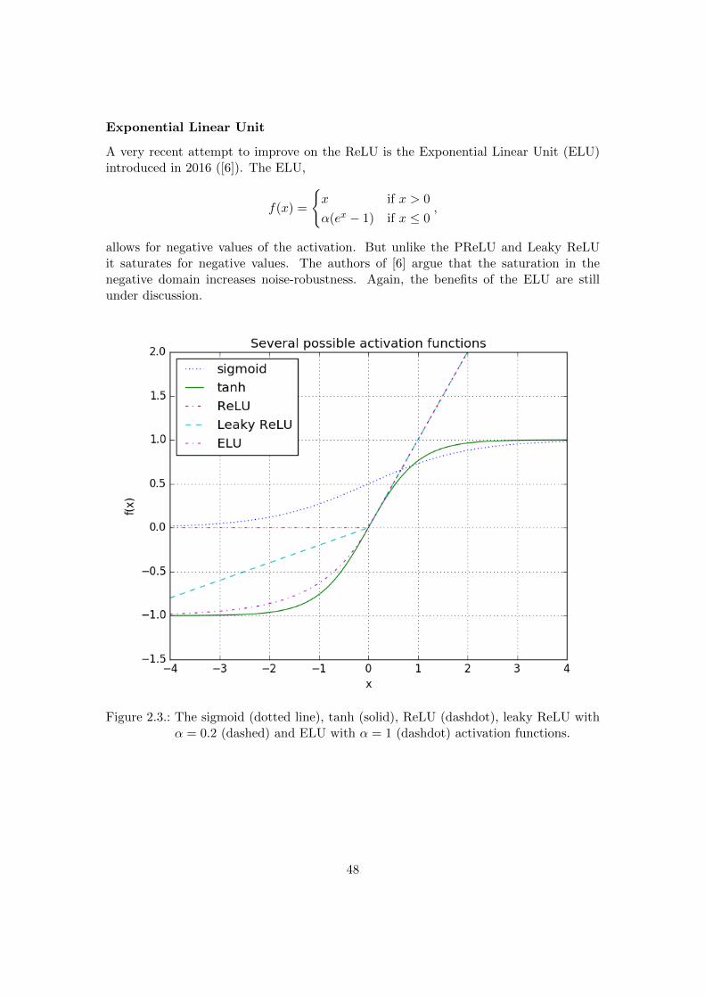
Exponential Linear Unit
A very recent attempt to improve on the ReLU is the Exponential Linear Unit (ELU)introduced in 2016 ([6]). The ELU,
f(x) =
x if x > 0
α(ex − 1) if x ≤ 0,
allows for negative values of the activation. But unlike the PReLU and Leaky ReLUit saturates for negative values. The authors of [6] argue that the saturation in thenegative domain increases noise-robustness. Again, the benefits of the ELU are stillunder discussion.
Figure 2.3.: The sigmoid (dotted line), tanh (solid), ReLU (dashdot), leaky ReLU withα = 0.2 (dashed) and ELU with α = 1 (dashdot) activation functions.
48

2.6. Weight initialization
Because an artificial neural network learns by adapting the weights and biases, theinitialization of these parameters is very important. A wrong initialization may lead tovery slow learning or no convergence at all, e.g. in the case of ReLU activation if themajority of neurons is dead after initializing or for sigmoidal functions if many neuronsinitialize in the tails.For a long time, people working with artificial neural networks used heuristic initializa-tion methods. Most commonly initializing the biases at zero and drawing each weightindependently from a normal distribution. By drawing them this way, they are all dif-ferent and centered around zero, improving the learning speed in the case of a tanhactivation function. The normal distribution was sometimes truncated to prevent largeweights, which can drive the neuron into saturation upon initialization. Because thevariance of the activation of layer l scales with dl−1, the number of neurons in the layerbefore it (see derivation below, equation (2.13)), the standard deviation of the the dis-tribution from which the weights are drawn is often taken to be inversely proportionalto the square root of dl−1. A similar scaling, but with dl, the number of neurons inlayer l, happens when updating the weights during backpropagation. For artificial neu-ral networks with symmetric activation function, Glorot and Bengio [10] introduced the‘Xavier’ initialization method in 2010. Compromising between reducing the variance ofthe output and the variance of the weights when backpropagating, their method comes
down to drawing the weights independently from a Uniform[−√6√
dl−1+dl,
√6√
dl−1+dl] distri-
bution. The Xavier method is still widely used, but more recently He et al. (2015 [13])used a reasoning similar to Glorot and Bengio to find an initialization method especiallyfor ReLU, LReLU and PReLU networks. We will explain the derivation of their methodbelow.
2.6.1. ReLU initialization
Just as the Xavier method, the ReLU weight initialization of [13] aims to prevent thescaling of the variance of the output when forward propagating, and the variance in theweights when backpropagating. This is especially important when working with deepand large network structures. We will do the derivation for a Leaky ReLU network(2.11), because setting α = 0 will cover the case of the ReLU.
Variance when forward propagating
Recall from Section 2.1 that the weighted input of layer l with dl nodes in a neuralnetwork is given by z(l) = W (l)a(l−1) + b(l), where z(l),b(l) ∈ Rdl , a(l−1) ∈ Rdl−1 andW (l) ∈ Rdl×dl−1 . The activation of this layer was defined as a(l) = σ(z(l)), where σ isthe activation function that is applied element-wise.We start with initializing the biases to zero, b(l) = 0, and for now take the weights,the entries of W (l), iid symmetrically around zero. In [13] the assumption is made thatthe entries of a(l−1) are also iid and a(l−1) and w(l) are independent. Because we are in
49
the initialization phase and no learning has taken place yet, the second assumption isreasonable. However, the independence of the elements in a(l−1) seems to be invalid in aneural network where every node in layer l− 1 is connected to every node in layer l− 2.Fortunately, they are identically distributed and because of the zero mean independently
initialized weights, the elements w(l)ji a
(l−1)i , i = 1, . . . , dl−1, have zero covariance among
each other and we can still split the variance of a sum into the sum of variances.The variance of weighted input j of layer l is given by
Var(z(l)j ) = Var
dl−1∑i=1
w(l)ji a
(l−1)i
=
dl−1∑i=1
Var(w(l)ji a
(l−1)i )
= dl−1Var(w(l)j1 a
(l−1)1 )
= dl−1
(Var(w
(l)j1 )Var(a
(l−1)1 ) + Var(w
(l)j1 )(Ea(l−1)1
)2+ Var(a
(l−1)1 )
(Ew(l)
j1
)2)= dl−1Var(w
(l)j1 )E
[(a
(l−1)1 )2
](2.12)
To calculate the expectation of the square of the activation, we need to realize that
a(l−1)1 = σ(z
(l−1)1 ). Because the biases initialization at 0 and the zero centered symmet-
rical weights, we see that z(l−1)1 is also symmetrically distributed around zero. Let us
denote its density function by fz. Then by symmetry
E[(a
(l−1)1 )2
]= E
[σ(z
(l−1)1 )2
]=
∫ 0
−∞fz(x)α2x2 dx+
∫ ∞0
fz(x)x2 dx
=1
2(1 + α2)E
[(z(l−1)1
)2]=
1
2(1 + α2)Var(z
(l−1)1 ).
Plugging this into equation (2.12) gives
Var(z(l)j ) =
1
2(1 + α2)dl−1Var(w
(l)j1 )Var(z
(l−1)1 ). (2.13)
In an artificial neural network with L layers and linear output function, we thereforefind that the variance of the output is
Var(yj) = Var(z(L)j ) = Var(z
(1)1 )
L∏l=2
(1
2(1 + α2)dl−1Var(w
(l)j1 )
)
= d0Var(x1)Var(w(1)j1 )
L∏l=2
(1
2(1 + α2)dl−1Var(w
(l)j1 )
),
50

where d0 is the number of inputs of the network. The last equality is because the input
layer does not apply any activation function, hence z(1)j is just the sum of the weights
times network inputs. Because the aim of the initialization method is to make sure thatthe variance of the input is not magnified or diminished exponentially in the output, theweights should be initialized such that
1
2(1 + α2)dl−1Var(w
(l)ji ) = 1, (2.14)
for all l, j, i. The method therefore suggests all weights to be initialized independentlyfrom a normal distribution with zero mean and variance 2/(dl−1(1 + α2)) to reduce theeffect of the number of neurons on the variance of the output. To be precise, we shouldhave chosen the variance for the weights in the first layer to be 1/d0, however, the authorsof [13] argue that dividing by a factor 1
2(1 + α2) will not be a big problem, since it onlyappears in one of the layers.
Variance when backpropagating
To avoid diminishing or magnification of the gradients when doing backpropagation, weargue along the same lines, but deviate a little from [13].Recall from equation (2.8) that
δ(l)j = σ′(z
(l)j )
dl+1∑i=1
w(l+1)ij δ
(l+1)i . (2.15)
In our case, σ′(x) = 1 if x ≥ 0 and σ′(x) = α when x < 0. Again we make assumptions
of independence between the weights wl+1ij and δ
(l+1)j and σ′(z
(l)j ). As in the case of
forward propagation, due to the symmetrical mean-zero initialization of the weights, z(l)j
is symmetrically distributed around 0. This means that E[σ′(z(l)j )2] = 1
2(1 + α2), thesame factor as showed up before. By the iid assumptions, taking the expectation ofequation (2.15) results in
E[δ(l)j ] = E[σ′(z
(l)j )]
dl+1∑i=1
E[w(l+1)ij ]E[δ
(l+1)i ] = 0.
Therefore, the variance becomes
Var(δ(l)j ) = E[
(δ(l)j
)2] = E[σ′(z
(l)j )2]E
dl+1∑i=1
w(l+1)ij δ
(l+1)i
2=
1
2(1 + α2)dl+1E[
(w
(l+1)1j
)2]E[(δ(l+1)1
)2]
=1
2(1 + α2)dl+1Var(w
(l+1)1j )Var(δ
(l+1)1 ),
51
a similar kind of iterative expression as in the forward propagation case! Now, for anetwork with L layers, we find in the first layer
Var(δ1j ) = Var(δ(L)1 )
L∏l=2
(1
2(1 + α2)dlVar(w
(l)1j )
). (2.16)
To mitigate effects on the variance of the error due to the number of neurons and layers,we can choose the weights such that
1
2(1 + α2)dlVar(w
(l)ij ) = 1, (2.17)
for all l, j, i. The difference between this case and the forward propagation case is thefactor dl instead of dl−1. In this case it would result in a normal distribution with meanzero and variance 2/(dl(1 + α2)).The authors of [13] note that it does not matter much whether one uses equation (2.14)or equation (2.17) to choose the variance of the weights. This is especially true whenthe layers are designed with the same number of nodes. In case one uses equation (2.14)and initializes the weights from a normal distribution with zero mean and variance2/(dl−1(1+α2)), the product term in equation (2.16) becomes dL/d1. Because this termis not dependent on the number of layers in the network, making the network deeper willnot have exponential effects on the variance. In [13] it is also empirically verified thatin both cases the neural networks converge to the correct target function. In practice,most networks are chosen to initialize according to equation (2.14).
2.7. Reduction of overfitting
Because every node in layer l of a neural network is connected to every other node inlayer l−1, the number of trainable parameters in even a relatively small network is fairlylarge. To illustrate this, a neural network with four hidden layers with fifty neurons ineach of them has a total of 9000 weights and 224 biases that have to be optimized tomatch the targets on the data. And there are many networks that are much larger. Inimage recognition tasks, neural networks with 5 to 60 million learnable parameters arenot uncommon [37]. This means that there is a serious risk of overfitting if the amountof training data is small. In that case, the network might learn noise in the data insteadof just the underlying trends. Such an overfitted network will perform very well on thetraining data, but poorly on unseen data (with different noise) and is therefore likely tohave a big error when used on a new data set. This makes it very important to keep trackof possible overfitting during training. When overfitting does occur, the easiest way tocombat it, is to reduce the size of the network (less layers and hidden neurons, thusless weights and biases), or to collect more training data. However, sometimes smallernetworks fail to capture complex relationships and more data is not available. In thesecases, there are many other methods to reduce or signal overfitting. In this section wewill only discuss the methods used or considered in the simulations in Chapter 3.
52

Separating training, validation and test data
Splitting the available data set is probably the method to signal overfitting that is mosteasy to implement. From the initial data set, roughly two-thirds is used as the trainingdata. The remaining data is split in half: one part validation data, one part test data.The network is trained on the training data. After each epoch, the network will berun on the validation data. Because the network did not train on the validation data,the error on this data set is likely to be bigger than on the training data. However ifthe difference is too large, it is probable that the model is overfitting the training data.Another indication that overfitting is happening is when the error on the training datadecreases, but the error on the validation data starts to increase.When determining the optimal network structure, there are more parameters to choosethan just the weights and biases. These are the so-called meta-parameters. Possiblemeta-parameters are the number of hidden layers, the number of hidden nodes per layer,the learning rate, the slope on the negative axis for Leaky ReLU activation functions,and so on. Other choices that have to be made when designing a network structureare the activation functions, the output function and the optimization and initializationmethods. Because looking at a network’s performance on the validation data and adapt-ing the meta-parameters to increase performance is also a form of ‘learning’, even in thisprocess there is a risk of overfitting. To see if this indeed is the case, the test data wasleft untouched. Only in the end, after the final network architecture has been selected,the network is run on the test data. This data set should therefore only be used once,and just to signal if there has been ‘manual’ overfitting on the validation data.A problem with this method of separating data arises when the data set is too small tosplit the data and train the network properly on the training data. Splitting on smalldatasets also increases the risk of ending up with a validation or training set that isnot representative of the whole data set. When selecting a network model with smalldatasets, an alternative method is k-fold cross-validation. The dataset is split into kparts of equal size. Then, k − 1 of these sets will be selected and used as training data.The remaining set is used as validation set. This is done k times, each time with adifferent set used as validation data. The validation error is taken as the average overthe k validation errors. This way, all of the data is used to train on and select a networkstructure. The size of k depends on the application and the amount of data, but typicallyk is taken to be ten.
Early stopping
Closely related to the method of separating training, test and validation data, is themethod of early stopping. Splitting the data will help signal overfitting. Early stoppingsimply means stopping the training when there are indications that overfitting mightoccur. This way the network will stop training when it has learned the most generalfeatures, but before it starts learning peculiarities or noise in the training data.
53

Regularization
A different approach to combat overfitting, is weight regularization. This method addsan extra term to the cost function, reducing the size of the weights. A common regu-larization term is the sum of the squared weights. In the case of cross-entropy, the costfunction becomes
C = −dL∑i=1
ti log(yi) +λ
2
∑w
w2,
where λ is called the regularization parameter. Since the training algorithm aims tominimize the cost function, adding this extra term will force the weights to be smaller.If the weights are smaller, the network output will change less when the input valueschange. Hence, fluctuations due to noise will have a smaller effect on the output. Thealgorithm will increase the size of a weight only when it significantly reduces the originalcost function. Note that the regularization parameter λ is also a meta-parameter that hasto be selected. Often regularization is used together with the other methods discussedin this section.
54

3. Simulations
The goal of this project was to use artificial neural networks to create a new prepaymentmodel to estimate prepayment probablities for groups of clients. The first section ofthis chapter describes what data was used to predict mortgage prepayments and how anoptimal network architecture was chosen. In the second section, the performance of theselected model is stated. All calculations were done in Python. To be able to work withartificial neural networks, Google’s open-source software library TensorFlow r0.12 wasused.
3.1. Method
We will first describe the data collection and pre-processing. We will explain shortlyhow to price the prepayment option and then a short description of the model selectionis given.
3.1.1. Data collection
The mortgage data used in the simulations is a small selection of the mortgage datafrom ABN AMRO. Because client data is very sensitive information, clients with similarmortgages are grouped into so-called buckets which are entirely anonymized. Againdue to data sensitivity, we only had access to 12 000 buckets to create our ‘portfolio’when writing this thesis. The mortgage start dates for the buckets range from 1970to 2016 and the interest reset dates from 2017 up to 2046. Besides the start and enddates, each bucket contains information about the interest rate on the loan (coupon),the amortization type, whether the client is an employee of ABN AMRO or not, if themortgage was ABN AMRO main brand or not, if the mortgage has a reconsider option,the length of the fixed interest period (term) and the amount of money of all clientsin the buckets combined (face amount). The face amount was not used to train thenetwork, only to price the prepayment option (Subsection 3.1.3).The components of the input data concerning the classification of a bucket into more thantwo classes, being amortization type (bullet, level, linear) and season, were presented inso-called ‘one-hot encoding’. For the amortization type, this means that it is transformedinto an array of length three, with a one on the location of its type and zeros elsewhere.For example for a bullet bucket, the amortization type is [1, 0, 0]. If the classeswhere given as a scalar with different values, say 1=bullet, 2=level, 3=linear, then levelwould be the average of bullet and linear, which is not the case. To remove these wrong‘closeness’ implications in the data, one-hot encoding is used. Every element of the
55
amortization type and season has its own input neuron, and the network can thereforebe trained without wrong preconceptions in the data. This brings the total number ofinput variables to 24: ten explanatory variables from which two in one-hot encoding andan indicator such that the network knows when a mortgage has a reconsider option.To calculate the HPI ratio, the HPI for each month from 1995 to 2016 in the Netherlandswas taken from Statistics Netherlands (CBS)1. For the 20 buckets with start dates before1995, the HPI of January 1995 was used to calculate the HPI ratio. From 2012 onward,the ABN AMRO HPI forecast was used. This forecasts predicts the HPI for each monthup to the end of 2044.To be able to progress the portfolio through time and calculate the interest incentives,short rate scenarios were run. As mentioned in Section 1.3, the mortgage rates are swaprates plus a service spread. To find the size of the service spread, we took the currentmortgage rates from the ABN AMRO website and compared them to the ICE swaprates2 with the same maturities. The mortgage maturities offered by ABN AMRO are1, 2, 3, 5, 6, 7, 10, 12, 15, 17, 20, 25 and 30 years.The Nelson-Siegel-Svensson parameters were taken from the ECB website3 for 1 De-cember 2016, from which the initial instantaneous forward curve and the zero couponbond prices were constructed as described in Subsection 1.3.3. The one-factor Hull-White model was then chosen to match the initial term structure in the way describedin Subsection 1.3.2.As a sanity check for the simulated short rates, a large amount of sample paths wasgenerated. As described in Subsection 1.3.1 about the Hull-White model, the short rateis normally distributed with mean and variance at time t given by
E[r(t)] = α(t), Var(r(t)) =σ2
2a
(1− e−2at
).
It turns out that the sample mean and sample variance are very close to the theoreti-cal mean and variance in all combinations of parameters tried. Plotting the empiricaldistribution function against the theoretical cumulative distribution function (Matlabnormplot), Figure 3.1, also shows normality of the generated sample paths.Confident that the generated short rate sample paths are correct, we generated 100sample paths of monthly swap rates up to 10 years in the future, with maturities thatare offered by ABN AMRO for mortgage loans. Using these and the HPI forecast, moredata was generated from the initial sample by simply progressing the portfolio throughtime with time steps of 7 months on each sample path (thus updating the remaininginterest period, interest incentive, loan age, penalty proxy, HPI ratio and season eachtime step). We chose time steps of 7 months to keep the size of the data manageableand make sure every month appears in the sampled data, which is important, since theseason is an explanatory variable. To reduce the amount of samples that are very alike,
1Base year 2010, http://statline.cbs.nl/Statweb/?LA=en2https://www.theice.com/iba/historical-data3https://www.ecb.europa.eu/stats/financial_markets_and_interest_rates/euro_area_yield_
curves/html/index.en.html
56
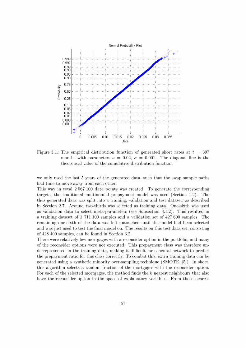
Figure 3.1.: The empirical distribution function of generated short rates at t = 397months with parameters a = 0.02, σ = 0.001. The diagonal line is thetheoretical value of the cumulative distribution function.
we only used the last 5 years of the generated data, such that the swap sample pathshad time to move away from each other.This way in total 2 567 100 data points was created. To generate the correspondingtargets, the traditional multinomial prepayment model was used (Section 1.2). Thethus generated data was split into a training, validation and test dataset, as describedin Section 2.7. Around two-thirds was selected as training data. One-sixth was usedas validation data to select meta-parameters (see Subsection 3.1.2). This resulted ina training dataset of 1 711 100 samples and a validation set of 427 600 samples. Theremaining one-sixth of the data was left untouched until the model had been selectedand was just used to test the final model on. The results on this test data set, consistingof 428 400 samples, can be found in Section 3.2.There were relatively few mortgages with a reconsider option in the portfolio, and manyof the reconsider options were not executed. This prepayment class was therefore un-derrepresented in the training data, making it difficult for a neural network to predictthe prepayment ratio for this class correctly. To combat this, extra training data can begenerated using a synthetic minority over-sampling technique (SMOTE, [5]). In short,this algorithm selects a random fraction of the mortgages with the reconsider option.For each of the selected mortgages, the method finds the k nearest neighbours that alsohave the reconsider option in the space of explanatory variables. From those nearest
57

neighbours, a sample of size N is drawn. For each of these N selected points, a newreconsider sample is created with explanatory variables equal to a random spot on theline between the original point and the selected neighbour.It turned out that this was beneficial for the performance of the neural network whenonly a subset of the data was used to train on. When training on a set of 2400 bucketsand the data points corresponding to the time evolution on 20 short rate sample paths,using the SMOTE algorithm on 50% of the reconsider mortgages with k = 1 and N = 1improved the prediction performance of the reconsider class. This smaller dataset wasused to roughly select the form of the final model.In the final model with the full data set derived from all 12 000 buckets, the network per-formed best without SMOTEd data. Apparently there were already sufficient reconsideroptions in the larger dataset to take this class into account.The magnitude of the different components of the data was very different. For example,the interest period start data is in the MATLAB date format, which is a number of theorder 105, while interest incentive is a percentage. To prevent the network from focusingthe learning process on the very large input values, it is recommended to normalize thedifferent inputs (e.g. in [11]). Therefore, we calculated the mean and standard deviationin the training set of each input type. Then, for the training, validation and test data,we used these to normalize the inputs. It is important to use the training data mean andstandard deviation to scale the test and validation data, because the validation data,test data and possible real-life datasets when applying the model may not contain thesame kind of samples in the same amount as the training data. After scaling, all inputtypes are of similar size such that the network is not biased towards the input with thelargest magnitude.
3.1.2. Model selection
Since the network aims to predict the prepayment probabilities over 6 classes, the net-work needs to have 6 output neurons. The total number of different inputs per bucketsis 24, so the network has 24 input neurons. We first select the output function and costfunction. Then number of hidden layers and the number of neurons per layer. Afterthat, the optimal activation function and learning rate are chosen. All decisions involveda lot of trial and error on the smaller data set with 2400 buckets (with extra SMOTEreconsider buckets). On this smaller set, the most promising network structures wereselected. It is convenient to do this on the smaller set, because of the smaller trainingtime (approximately 15 minutes). However, we can only judge the performance of anynetwork structure on the full data set. On a small dataset, it is difficult to measure theperformance of larger networks, because they are more likely to be overfitted. There-fore, to select the final model, the most promising candidates were also tried on the fulldataset of 12 000 buckets. Of course, the networks were trained on the training dataand performance was measured on the validation data. Training on this large datasettook slightly less than two hours, but the exact training time depended on the size ofthe network. The test data was left untouched. Surprisingly, on the full dataset therewere no signs of overfitting. Therefore, we did not apply regularization by penalizing
58

large weights (as described in Section 2.7).
Output and cost function
Even though estimating the prepayment probabilities per prepayment class is in fact aregression problem, we noticed that using the cross-entropy cost function in combinationwith softmax output function performed significantly better than minimizing the meansquared error (both with linear output as with softmax output function). This is mostlikely due to the fact that there is a big difference in magnitude of the six prepaymentclasses. By the nature of the MSE, minimizing it will focus on absolute differencesbetween the network output and the targets,
∂
∂yj
(1
2‖y − t‖2
)= yj − tj .
This means that a big difference in magnitude of the output neurons will lead to lessoptimization to minimize the error of the smaller output nodes. In our case, for example,the prepayment probabilities for the category relocation are roughly between 10−4 and10−2, while the magnitude of the reconsider probability may exceed 0.15. This differencemakes it difficult for the MSE to converge on the relocation class.On the other hand, the cross-entropy error will take into account the relative error,
∂
∂yj
(dL∑i=1
ti log(yi)
)=tjyj,
thus paying more attention to the smaller output neurons. In an attempt to fix thisproblem for the MSE, we tried dividing each component of the squared error by theaverage of the target ti, resulting in a derivative of
∂
∂yj
(1
2
dL∑i=1
(yi − ti)2
ti
)=yi − titi
.
Minimizing this weighted MSE outperformed the normal MSE in predicting the smallerprepayment classes correctly. However, because the cross-entropy error still resulted infaster convergence we chose to work with cross-entropy and softmax output. However,we only used the cross-entropy error in the optimization. To document the predictionerror, we will still use the MSE and also look at the relative error per prepayment class,because it is more insightful.
Optimization method and number of hidden layers and hidden neurons
On the smaller data set, it was immediately clear that the Adam optimization method,discussed in Subsection 2.3.3, yielded the best network performance. We therefore choseto work with this optimizer. Even though the article introducing Adam is still in preprint,this optimization method is already widely used throughout the field of neural networks.
59

The networks that showed the most promising results on the smaller dataset, consistedof either 1 hidden layer with with around 125 neurons or 4 hidden layers with 50 neuronseach. Therefore, we explored several network architectures close to these two shapes onthe large dataset. In the tests, a Leaky ReLU activation function (α = 0.2), softmaxoutput and CE cost function were used. The number of epochs may vary due to earlystopping (Section 2.7), but was set to 200 if no stopping occurred. To reduce the impactof the initialization and random effects, the average over 5 training sessions is taken.Some of the results are listed in Table 3.1.
Results on validation data
hidden layers xnodes
MSE (×10−8)
1×125 5.6831×130 7.6154×50 2.7084×60 23.894×100 2.3275×50 5.9297×50 5.20410×35 8.085
Table 3.1.: The MSE on the validation data of the full data set for networks with LeakyReLU activation function, learning rate 0.001, softmax output and CE costfunction, averaged over 5 training sessions.
Activation function
To find the best performing activation function, we used a network with 4 hidden layersof 50 hidden neurons each. Some results on the validation data are listed in Table 3.2.
Results on validation data
Activation function MSE (×10−8)
LReLU α = 0.01 4.219LReLU α = 0.1 9.345LReLU α = 0.2 2.708LReLU α = 0.3 3.483PReLU 3.896ReLU 5.780ELU 9.100
Table 3.2.: The MSE on the validation data of the full data set for networks with 4hidden layers with 50 nodes, learning rate 0.001, softmax output and CEcost function, averaged over 5 training sessions.
60
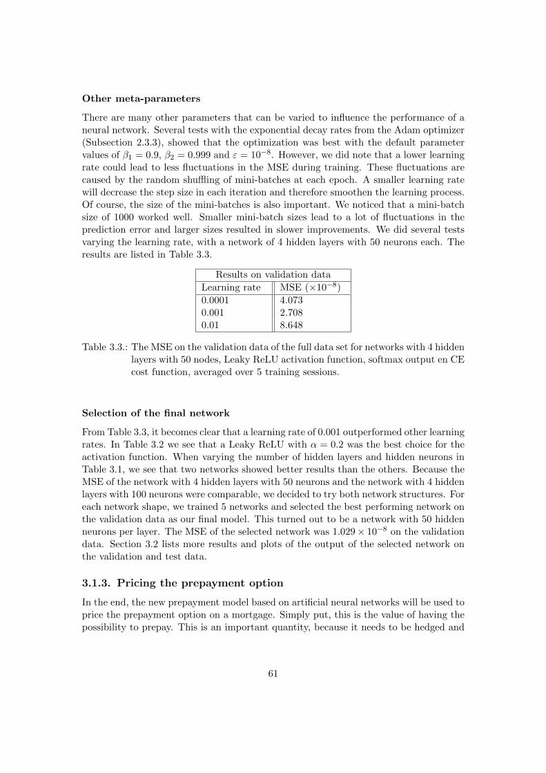
Other meta-parameters
There are many other parameters that can be varied to influence the performance of aneural network. Several tests with the exponential decay rates from the Adam optimizer(Subsection 2.3.3), showed that the optimization was best with the default parametervalues of β1 = 0.9, β2 = 0.999 and ε = 10−8. However, we did note that a lower learningrate could lead to less fluctuations in the MSE during training. These fluctuations arecaused by the random shuffling of mini-batches at each epoch. A smaller learning ratewill decrease the step size in each iteration and therefore smoothen the learning process.Of course, the size of the mini-batches is also important. We noticed that a mini-batchsize of 1000 worked well. Smaller mini-batch sizes lead to a lot of fluctuations in theprediction error and larger sizes resulted in slower improvements. We did several testsvarying the learning rate, with a network of 4 hidden layers with 50 neurons each. Theresults are listed in Table 3.3.
Results on validation data
Learning rate MSE (×10−8)
0.0001 4.0730.001 2.7080.01 8.648
Table 3.3.: The MSE on the validation data of the full data set for networks with 4 hiddenlayers with 50 nodes, Leaky ReLU activation function, softmax output en CEcost function, averaged over 5 training sessions.
Selection of the final network
From Table 3.3, it becomes clear that a learning rate of 0.001 outperformed other learningrates. In Table 3.2 we see that a Leaky ReLU with α = 0.2 was the best choice for theactivation function. When varying the number of hidden layers and hidden neurons inTable 3.1, we see that two networks showed better results than the others. Because theMSE of the network with 4 hidden layers with 50 neurons and the network with 4 hiddenlayers with 100 neurons were comparable, we decided to try both network structures. Foreach network shape, we trained 5 networks and selected the best performing network onthe validation data as our final model. This turned out to be a network with 50 hiddenneurons per layer. The MSE of the selected network was 1.029× 10⁻⁸ on the validationdata. Section 3.2 lists more results and plots of the output of the selected network onthe validation and test data.
3.1.3. Pricing the prepayment option
In the end, the new prepayment model based on artificial neural networks will be used toprice the prepayment option on a mortgage. Simply put, this is the value of having thepossibility to prepay. This is an important quantity, because it needs to be hedged and
61

is used in the calculations of the penalty on the prepayment classes curtailment highand refinancing. We can calculate the price of the prepayment option by calculatingthe difference between the value of the interest payments (coupon times face amount atthe specific time) on a bucket with prepayments and without prepayments. All futureinterest payments have to be discounted to determine the present value of the mortgageloan with and without prepayments.To quantify the performance of the neural network compared to the multinomial prepay-ment model, we calculate the value of the interest payments for mortgage loans withoutprepayment, with prepayment as predicted by the multinomial model and as predictedby the neural network. To do this, scenarios are generated as described in Subsection3.1.1. Portfolios are progressed through time and the discounted interest cash flows arecalculated for the three cases. Because the outstanding loan in a bucket is gigantic andalso differs per bucket, we will look at the price of the prepayment option relative to thevalue of the mortgage without prepayments.
3.2. Results
In this section we will state and discuss the results of the model selected in Subsection3.1.2 on the test data. This dataset has not been used in any way in earlier stages. Theexpectation is therefore that the network will perform slightly worse on this data setcompared to its performance on the validation data.The best performing network achieved a mean squared error on the validation data of1.029× 10−8, while the error on the training data was 9.333× 10⁻⁹. Plotting the MSEon both training and validation data during training on a logarithmic scale, results inFigure 3.2.As we can see, the error fluctuates a lot due to the stochastic shuffling of mini-batches.However, by applying the early stopping method we are able to stop training when theMSE is at a minimum. The large fluctuations could point to a mini-batch size that istoo small or a learning rate that is too large. However as the experiments in Subsection3.1.2 describe, varying these did not improve the approximations. Another way to trackthe effectivity of a network is to look at the values of the activations per layer. If toomany activations are negative, the network will learn slowly from that point on dueto the smaller gradient of the Leaky ReLU activation function in the negative domain.Histograms of the average activations per neuron in each layer are shown in Figure 3.3.As we can see, the first two layers show many activations in the positive domain, thus thelearnable part of the Leaky ReLU. In the last two layers, activations tend to accumulatearound 0. This is not optimal, but because we are using a Leaky ReLU neuron, it is nota real obstacle if we want to continue learning, since we chose the negative slope to beα = 0.2; sufficient to recover from dying neurons.To visualize the performance of the network on the validation data, we can plot thenetwork predictions for a couple of buckets and compare them to the targets. This isdepicted in Figure 3.4.These plots show that the prepayment probabilities are predicted well in most cases.
62

Figure 3.2.: The MSE on logarithmic scale of the prepayment predictions of a neuralnetwork with 4 hidden layers with 50 hidden neurons each, Leaky ReLU(α = 0.2) activation function and softmax output. The green line is theMSE on the training data, the blue line on the validation data.
This also shows from the relative error per prepayment class on the validation data,presented in Table 3.4.Another way to visualize the results is by using scatter plots. This is done in Figure 3.5.As we can see, the predictions of the neural network agree very well with the targets.Especially if taken into account that there are 1 711 100 data points in the training dataplot and 427 600 in the validation data plot.Finally we are allowed to use the test data. It turned out that the model did indeedperform worse on the test data, having a MSE of 3.995× 10⁻⁸. The relative errors perprepayment class are given in Table 3.5.As we can see, the average relative errors per prepayment class are the same as those onthe validation data. The scatter plot on the test data is shown in Figure 3.6.As we can see, there are slightly more outliers in the scatter plot of the test data, butagain, taking into account that there are 428 400 data points in the scatter plot, the
63

Figure 3.3.: Histograms of the average activations in each layer for the neural networkprepayment model on the training data.
result is satisfying since the neural network seems to be able to capture the generalrelation between the explanatory variables and the target prepayment predictions.When using the model to calculate the price of the prepayment options on mortgages,we generated another 200 short rate sample paths and evaluated 200 buckets. We foundan average difference of 0.42 % compared to the prepayment options priced with themultinomial model.
64

refinancing relocation reconsider curt. high curt. low no event
0.51 % 0.58 % 1.00% 0.56 % 1.02 % 0.0098 %
Table 3.4.: The average relative error per prepayment class of the neural network on thevalidation data.
refinancing relocation reconsider curt. high curt. low no event
0.51 % 0.58 % 1.00% 0.56 % 1.02 % 0.0098 %
Table 3.5.: The average relative error per prepayment class of the neural network on thetest data.
Figure 3.4.: Four plots of the predicted prepayment probability per prepayment class(blue) compared to the target prepayment probabilities (red) on randombuckets. On the y-axis we see the prepayment probabilities, on the x-axisthe prepayment categories number as numbered in Section 1.1 (category 6:no event is left out since it is determined by the other 5 and is a lot largerthan the other probabilities). The lines coincide almost perfectly.
65
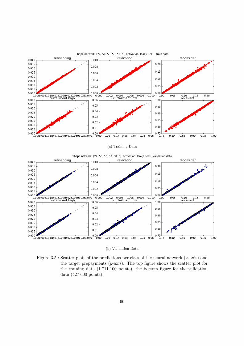
(a) Training Data
(b) Validation Data
Figure 3.5.: Scatter plots of the predictions per class of the neural network (x-axis) andthe target prepayments (y-axis). The top figure shows the scatter plot forthe training data (1 711 100 points), the bottom figure for the validationdata (427 600 points).
66
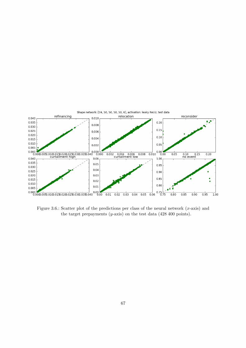
Figure 3.6.: Scatter plot of the predictions per class of the neural network (x-axis) andthe target prepayments (y-axis) on the test data (428 400 points).
67

4. Conclusion
It has become clear from the results in Section 3.2, that the selected artificial neuralnetwork with 4 hidden layers of 50 neurons each was able to capture the underlyingrelation between the explanatory variables and the generated prepayment targets. Thisdoes vouch for the use of these kind of networks in prepayment modelling. However, wemust note that the errors were still large.We stress the importance of using enough data during the training phase of a network,as the errors might have been smaller if a larger number of different short rate samplepaths had been present in the training data. Another important thing to keep in mindis that if a network is supposed to perform in extreme situations, also a number ofdata points in this extreme domain should be added to the training data. This is vital,because networks are poor extrapolators and it is especially difficult to predict theiroutcome on data that is very different from the data they were trained on. One optionthat could be considered is using a neural network based model in combination witha traditional multinomial prepayment model. The neural network will function on thenormal domain, but in extreme scenarios that were not included in the training datathe multinomial model could take over. This also has the benefit that it is easier tounderstand the influence of input data on the output of the multinomial model.Although the estimation errors on the prepayment probabilities look small, even a smallerror can have big consequences because very large amounts of money are involved. Forthat reason, it is important to keep improving the model and keep training it on largeand recent datasets. For some other suggested directions of further research to improvethe models performance, see Section 5.2.Unfortunately, we did not have access to the real prepayment data. This means thatwe cannot draw any conclusions about the performance and applicability of the neuralnetwork based prepayment model on the real dataset. However, the estimation of theprepayment probabilities was accurate on the generated targets. This is promising. Theactual relation between the explanatory variables and the prepayment probabilities islikely to be a lot more complex than the one described by the multinomial prepaymentmodel. Because of the theoretical capacities of artificial neural networks to approximatevery complex functions it is likely that neural networks have the potential to be betterpredictors of prepayment than the current multinomial prepayment model. Especiallybecause large amounts of prepayment data have been collected and could be used fortraining in the future. Because of this potential of a model based on a neural network,we encourage further research in its applications to this and other models within ABNAMRO.We will expatiate on these recommendations in Section 5.1.
68
5. Discussion and Further Research
In the first section of this chapter, we discuss the general and problem specific advantagesand disadvantages of the use of neural networks in risk modelling. Section 5.2 suggestssome improvements to the selected model that might be promising. In Section 5.3 wewill shortly review the process of writing this thesis.
5.1. Advantages and disadvantages of artificial neuralnetworks
There are several advantages and disadvantages in the use of artificial neural networks.Below, we will summarize a few of them.
Data-driven
One of the main characteristics of artificial neural networks is that they will learn solelyfrom the data they are trained on. As we have shown in Section 2.2, they are universalapproximators and therefore, if a function describing the relation between the input dataand the targets exists, they are theoretically capable of approximating this function. Tobe able to train well, large quantities of data are necessary. This can be a restriction,but in this case of mortgage prepayments it is not. The selection of 12.000 bucketsavailable in writing this thesis, is just a tiny fraction of the total amount of data onmortgages. During training, the network may discover relations that the modeller is notyet aware of and no restrictive assumptions on the data are necessary to be convincedthat a neural network can capture the sought after relation. One only has to select anetwork architecture and have large amounts of data. The training will take care ofthe rest. Once trained, the network will be immediately applicable to new situations.However, it should be stressed that a neural network can only learn what it is shown.To be able to handle extreme situations such as stress tests, it should be trained on datawith explanatory variables in this extreme domain. If there is no training data availablein a certain domain, the network cannot be expected to extrapolate well as it is simplynot taught how to do so.That the network learns what it is shown, is also something one has to be careful withfor another reason. Especially if neural network output is used to make decisions about(individual) clients, it is very important to consider what kind of relations the network isallowed to find. If you feed it data including the ethnicity of clients, the network is verylikely to include this data in its decisions and might develop racist tendencies. In thiscase it is obviously not right to include ethnicity, but sometimes other apparently more
69

harmless input data may lead the network to similar results. If for example the addressof the client is used as an input parameter, the network might favour one neighbourhoodover the other. If one of these neighbourhoods has a high concentration of specific ethnicgroup, the results are virtually the same. Accidentally racist (or sexist) algorithmsappeared before with purely data-driven algorithms (e.g. [22]), and should serve as awarning. Think carefully about what explanatory variables you want the network tobase its decisions on and be aware of the possible consequences of feeding all availabledata to a neural network and let it figure out what to do by itself.
Rapidly developing field of research
New articles suggesting improvements on the shape of neural networks, the activationfunction, optimization method, weight initialization method and so on, seem to appearalmost every day. Considering the achievements already made with the current tech-niques, this is an indication that the performance of neural networks will increase in thecoming years. That is, if one keeps up with all the developments. In a field of researchthat moves this fast, the state-of-the-art models from this year may already be outdatednext year. This will force the modeller to constantly stay up to date with the mostrecent articles and try the new methods in his models. This can make working withneural networks time consuming, despite the fact that the concept is easily understood.However, we strongly recommend doing so. Using the ReLU weight initialization [13],introduced in 2015, and the Adam optimizer [16], introduced in 2017, greatly improvedthe performance of our neural network compared to older methods.
Other observations
When working with neural networks in risk modelling, several other factors have to betaken into account. One of those is that a network needs to be retrained regularly asnew data becomes available. The financial markets and client behaviour are dynamical,and their behaviour may change from year to year. Recent data should be added tothe training data and old irrelevant data (e.g. through regulatory changes) should beremoved.Another property of neural networks that became clear in doing this research, is thatthere is some randomness in how well a network learns. Performance may vary even whentraining on the same data and using the same validation data. To mitigate the variancein network results, an easy solution is to train several networks and pick the one thatperforms best on the validation data. The selected network should then be tested on thetest data to see whether it performs accordingly and did not just by chance match thevalidation data well. Another procedure one can consider is called ensemble averaging([12]). In this method, multiple neural networks are trained on the same dataset. Then,instead of using only one of the networks, a weighted average of the outputs is used. Theweights are determined by the performance of the individual networks on the validationdata (or can even be optimized using another neural network). In this thesis, we choseto work with just one neural network. However, each of the discarded networks may
70

have learned a different aspect of the training data, so if the estimation problem is morecomplex or if there are different classes of input data, ensemble averaging may be worthinvestigating.The last thing we want to touch upon in this section is what some call the ‘black box’property of neural networks. Input data goes in and the network gives output, butwhat happens in between is very difficult to decipher. This is because of the highlynon-linear form of the transformation of input data and the large amounts of weightsand biases (in our relatively small four hidden-layer network already 9224). This makesit difficult to track the impact of changing one of the input variables, meaning that aneural network trained for a specific problem can in most cases not tell the user generalrules regarding its decision-making. One could evaluate the output of the network on asurface of explanatory variables to visualize the impact of different inputs, but in highdimensional settings this is not very insightful. The only way to comfort the user (andpossible regulators) is to show the networks performance on test datasets.
5.2. Further research
In this section we will describe some possible improvements of the selected model, whichwe were not able to try due to time constraints.Because the data used to price the prepayment option was newly generated and thereforeunseen by the network, the error on the prepayment option might have been reduced bya larger number of different short rate sample paths in the training data. This could havereduced the probability of ‘surprising’ sample paths in the pricing of the option. Thisstresses the importance of a large training data set, so that the network is even moreable to capture the underlying general relation between explanatory variables and theprepayment probabilities. We are also aware of the fact that we trained the network onpredicting the prepayment probabilities, and not on predicting the correct value of theprepayment option. Although these two are closely related, it would be interesting tosee if a network is able to directly price the prepayment option, without first calculatingthe individual prepayment probabilities per category.Another observation when looking at the results in Section 3.2, is that we barely seesigns of overfitting. This is good, but it is also an indication that even larger networks(if necessary with regularization) can be applied to this problem. However, trying largernetworks did not yield better approximation results with our dataset. This could eithermean that the general relation between input and output is already captured by thisnetwork structure or that there is insufficient data to try larger networks. Whenever thetraining dataset will be taken bigger (which will be the case when working with the realprepayment data), we therefore encourage experimenting with larger network structures.
5.3. Review of the process
After choosing the subject of this research at ABN AMRO, I had a very pleasant timeworking there and being part of the team. I also got the possibility of doing the large
71

computations necessary to train neural networks on their server. I had a lot of freedomto determine my own working schedule and working hours. My daily supervisor, BastianWemmenhove, helped me to determine the direction of this research during our meetingsand would point me in the right direction when I needed it. Therefore, I would like tothank ABN AMRO and Bastian in particular for the support and encouragements duringthis research. I also want to thank Peter Spreij for his feedback on earlier versions ofthis thesis. Below I will reflect on some of the difficulties I encountered in the processof writing and doing research.One of the greatest difficulties was the unavailability of data. As mentioned in Subsection3.1.1, client data is difficult to get by. Even when anonymized and grouped in buckets,it was not possible to get the real prepayment data for this research. Therefore, targetshad to be created using the existing multinomial prepayment model. This means thatthe results only reflect the networks ability to replicate the other model. Even though itis encouraging that it could to a reasonable extent, before we can draw any conclusionsabout the applicability of this model, it should be trained and tested on real prepaymentdata.Another challenge in writing this thesis was that I was forced to use an older versionof TensorFlow (r0.12). Because this is such a rapidly evolving field, it is very useful tohave the most recent version of the software (this currently is r1.12). Because of theolder software, a functionality like early stopping was difficult to implement and savingtrained networks was not possible at all due to a bug. Luckily this has been fixed innewer versions of TensorFlow and I recommend updating the version at ABN AMRO tofacilitate further research in this topic.Because of the many advantages and the potential a model based on a neural networkhas, I encourage further research in the application of these networks to this and othermodels within ABN AMRO. Hopefully this thesis can function as a guide to developinga new prepayment model and help modellers get up to speed in the development ofother neural network models. With the large quantities of data the bank has collected,artificial neural networks definitively have the potential to add value to risk modelling.
72

Popular Summary
In this master thesis, we try to predict part of the risk for a bank when writing out amortgage loan. When a customer takes a mortgage loan of thirty year, but decides topay it back after only ten, the bank loses twenty years of interest payments. If you realizethat ABN AMRO has billions of euros of outstanding mortgage loans, it is not hard tosee why it is important for them to predict how many customers are going to pay backtheir loan before the end of the contract. There are many parameters that can influencethese so-called mortgage prepayments. Among others, think of the difference betweenthe interest rate the client is paying and the interest rate he can get on a new mortgage,the length of the contract or even whether the client is an employee of ABN AMROor not. In our research, we take into account 24 different parameters influencing theprobability of prepayment, among which the three mentioned above. We assume thereexists a function f that maps the data of the loan to the probability of prepayment.Because this is a real-world problem, we do not know what this function looks like orhow complicated it is (it may even change each year!), but we do want to approximateit. This is where the neural networks come into play.Artificial neural networks are booming. A lot of impressive recent developments, rangingfrom self-driving cars to Apple’s Siri, are thanks to these networks. How these artificialneural networks work is actually not so difficult to understand. Artificial neural networksare used as approximators. They can for example approximate the function taking animage of a handwritten number as input and giving the number it represents as output.Or in this thesis, the function taking the mortgage prepayment parameters as input andthe prepayment probability as output.In Figure 2 below we see a schematic representation a neural network. The input entersfrom the left, and the signal flows to the right. Each node in the network takes a weightedsum of all the input it receives, applies a certain function to it and sends it on to allneurons in the next layer. The key to making this neural network approximate the targetfunction, is to make it ‘learn’ the correct weights. It gets to see a lot of input values andmakes predictions. If the prediction was incorrect, all weights are changed a little in thedirection that will make the network give a better prediction next time.This way, the network learns by making mistakes. Much like our own brain! You canimagine that big neural networks with many layers and neurons are able to capture verycomplicated structures in the data. Indeed, it turns out that they are very good atrecognizing patterns in data. In this thesis we explore how we can use this potential topredict prepayment behaviour.
73
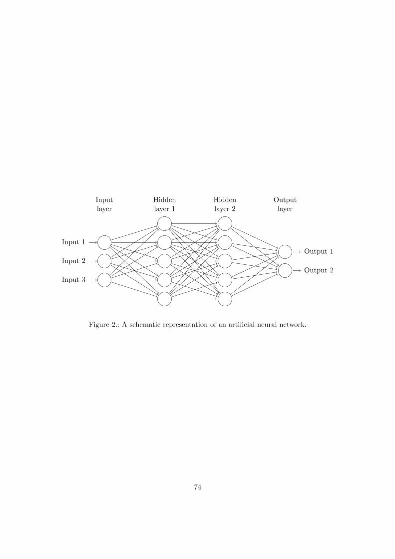
Input 1
Input 2
Input 3
Output 1
Output 2
Hiddenlayer 1
Hiddenlayer 2
Inputlayer
Outputlayer
Figure 2.: A schematic representation of an artificial neural network.
74

Bibliography
[1] R.A. Adams, J.J.F. Fournier, Sobolev Spaces, Academic Press, 2003
[2] C.M. Bishop, Pattern Recognition and Machine Learning, Springer-Verlag NewYork, Inc., 2006
[3] D. Brigo, F. Mercurio, Interest Rate Models - Theory and Practice, Springer-VerlagBerlin Heidelberg, 2007
[4] B. Brosowski, F. Deutsch, An Elementary Proof of the Stone-Weierstrass Theorem,Proceedings of the American Mathematical Society, Vol. 81, No. 1, pp. 89-92, 1981
[5] N.V. Chawla et al., SMOTE: Synthetic Minority Over-sampling Technique, Journalof Artificial Intelligence Research, Vol. 16, pp. 321–357, 2002
[6] D. Clevert, T. Unterthiner, S. Hochreiter, Fast and Accurate Deep Network Learningby Exponential Linear Units (ELUs), Published as a conference paper at ICLR,ArXiv:1511.07289v5, 2016
[7] G. Cybenko, Approximations by Superpositions of Sigmoidal Functions, Mathemat-ics of Control, Signals, and Systems, Vol. 2 (4), pp. 303-314, 1989
[8] W.F. Donoghue, Distributions and Fourier Transforms, Pure and Applied Mathe-matics, Vol. 32, 1969
[9] D. Filipovic, Term-Structure Models, Springer-Verlag Berlin Heidelberg, 2009
[10] X. Glorot, Y. Bengio, Understanding the Difficulty of Training Deep FeedforwardNeural Networks, Journal of Machine Learning Research: Proceedings of MachineLearning Research, Vol 9, pp 249-256, 2010
[11] M.T. Hagan et al., Neural Network Design (2nd Edition), http://hagan.okstate.edu/nnd.html, 2014
[12] S. Haykin, Neural Networks: A Comprehensive Foundation, Prentice Hall, 1998
[13] K. He et al., Delving Deep into Rectifiers: Surpassing Human-Level Performanceon ImageNet Classification, IEEE International Conference on Computer Vision(ICCV), arXiv:1502.01852v1, 2015
[14] K. Hornik, M. Stinchcombe, H. White, Multilayer Feedforward Networks are Uni-versal Approximators, Neural Networks, Vol. 2. pp. 359-366, 1989
75

[15] J.C. Hull, A. White, Pricing Interest Rate Derivative Securities, The Review ofFinancial Studies, Vol. 3 (4), pp. 573-592, 1990
[16] D.P. Kingma, J.L. Ba, ADAM: A Method for Stochastic Optimization, CoRR,preprint arXiv:1412.6980, v9 2017
[17] A. Krizhevsky, I. Sutskever, G.E. Hinton, ImageNet Classification with Deep Convo-lutional Neural Networks, NIPS’12 Proceedings of the 25th International Conferenceon Neural Information Processing Systems, pp. 1097-1105, 2012
[18] B. Kuijvenhoven, B. Maarse, E. Driessen, Dutch Residential Mortgage Interest -Typical Prepayment 7.0 Model, ABN AMRO, 2016
[19] Y. LeCun, Y. Bengio, G.E. Hinton, Deep Learning, Nature, Vol. 521 (7553), pp.436-444, 2015
[20] M. Leshno et al., Multilayer Feedforward Networks with a Nonpolynomial ActivationFunction Can Approximate Any Function, Neural Networks, Vol. 6, pp. 861-867,1993
[21] V.Y. Lin, A. Pinkus, Fundamentality of Ridge Functions, Journal of ApproximationTheory, Vol. 75 (3), pp. 295-311, 1993
[22] S. Lowry, G. Macpherson, A Blot on the Profession, British Medical Journal, Vol.296 (6623), pp 657–658, 1988
[23] A.L. Maas, A.Y. Hannun, A.Y. Ng., Rectifier Nonlinearities Improve Neural Net-work Acoustic Models, Proc. ICML, Vol. 30, 2013
[24] W. McCulloch, W. Pitts, A Logical Calculus of Ideas Immanent in Nervous Activity,Bulletin of Mathematical Biophysics, Vol. 5 (4), pp. 115–133, 1943
[25] C.R. Nelson, A.F. Siegel, Parsimonious Modeling of Yield Curves, The Journal ofBusiness, Vol. 6 (4), pp. 473-489, 1987
[26] M.A. Nielsen, Neural Networks and Deep Learning, Determination Press, 2015
[27] F. Pardoel, Penalty Model, ABN AMRO, 2015
[28] A. Pinkus, Approximation Theory of the MLP Model in Neural Networks, ActaNumerica, Vol. 8, pp 143-195, 1999
[29] A. Pinkus, Density in Approximation Theory, Surveys in Approximation Theory,Vol.1, pp. 1-45, 2005
[30] F. Rosenblatt, The Perceptron: A Probabilistic Model For Information Storage AndOrganization In The Brain, Psychological Review, Vol. 65 (6), pp. 386–408, 1958
[31] S. Ruder, An Overview of Gradient Descent Optimization Algorithms, CoRR,preprint arXiv:1609.04747, 2016
76

[32] W. Rudin, Real and Complex Analysis, McGraw-Hill Book Company, 1987
[33] D.E. Rumelhart, G.E. Hinton, R.J. Williams, Learning Representations by Back-Propagating Errors, Nature, Vol. 323, pp. 533–536, 1986
[34] B.P. Rynne, M.A. Youngson, Linear Functional Analysis, Springer-Verlag London,2008
[35] P.Y. Simard, D. Steinkraus, J.C. Platt, Best Practice for Convolutional NeuralNetworks Applied to Visual Document Analysis, Proceedings ICDAR, pp. 958–9622003
[36] L.E.O. Svensson, Estimating and Interpreting Forward Interest Rates: Sweden 1992-1994, Centre for Economic Policy Research, 1994
[37] C. Szegedy et al., Rethinking the Inception Architecture for Computer Vision,CoRR, preprint arXiv:1512.00567, 2017
[38] B. Vostrecov, M. Kreines, Approximation of Continuous Functions by Superposi-tions of Plane Waves, Dokl. Akad. Nauk SSSR, Vol. 2, pp. 1237– 1240, 1961
77

Appendices
78

A. Additional Theorems and Definitions
In this Appendix we will state theorems (if insightful with proofs) and definitions thatare referenced throughout the text.
A.1. Theorems for Chapter 1
This section will state results that are needed in Chapter 1. We will start with a recapmainly summarizing Chapter 2 in Filipovic ([9]) and Chapter 1 of Brigo and Mercurio([3]). Throughout this section, we assume (Ω,F ,P) to be a probability space withfiltration F = Ftt≥0 satisfying the usual conditions.
Bank account, short rate, discount factor, zero-coupon bond
The most basic definition in interest rates is the bank account. The bank account ormoney-market account satisfies the differential equation
dB(t) = r(t)B(t) dt, B(0) = 1,
such thatB(t) = e
∫ t0 r(s) ds.
Hence B(t) changes risk-free with the (stochastic) short rate r(t). The money-marketaccount is used to define the discount factor, determining the value at time t of moneyavailable at a time T > t. To discount an amount at time T to its value at time t wemultiply by the discount factor
D(t, T ) =B(t)
B(T )= e−
∫ Tt r(s) ds.
A definition closely related to the discount factor is that of the zero-coupon bond (tostress the maturity time T of a zero-coupon bond, it is also called a T -bond). A zero-coupon bond with maturity time T is a contract that pays 1 unit of currency at timeT . The price of this contract at time t < T is denoted by P (t, T ). The differencebetween the discount factor D(t, T ) and the price of a zero-coupon bond P (t, T ) is thatP (t, T ) has to be known at time t, since it is the price of a product, hence P (t, T ) isFt-measurable. While D(t, T ) is FT -measurable, since the future values of the short rateprocess r are not known at time t.If we also assume there exists an equivalent martingale measure Q, meaning that Q ∼ Pand all discounted price processes are martingales under Q, the market is arbitrage free
79

([9] Section 4.3) and the relation between the discount factor and the zero-coupon bondprice becomes
P (t, T ) = EQ
[e−
∫ Tt r(s) ds | Ft
]. (A.1)
Forward rate agreement and derived rates
Another basic financial product is the so-called forward rate agreement (FRA). At time
t, the buyer of this contract sells one T -bond an buys an amount of P (t,T )P (t,S) S-bonds. The
net investment is therefore 0. At time T he has to pay 1 unit of currency according tothe sold T -bond. At time S he receives P (t,T )
P (t,S) units of currency.The definition of this instruments leads to the definition of the simply compounded andthe continuously compounded forward rate. The simply compounded forward rate isdefined as
F (t;T, S) =1
S − T
(P (t, T )
P (t, S)− 1
). (A.2)
This is exactly the simple interest rate which makes a forward rate agreement fair. If weinvest one unit of currency at time T and we receive simple interest on the investment,at time S we have
1 + (S − T )F (t;T, S) =P (t, T )
P (t, S),
exactly the cash flow of the FRA. Simply compounded forward rates are widely used infinance. An important example of a simple forward rate is the London Interbank OfferedRate, in short LIBOR, which is the rate at which banks borrow money from each otherand the rate at which swaps between banks are traded.If we use continuously compounded interest rates, the rate to make the forward rateagreement fair is the rate R(t;T, S) such that
eR(t;T,S)(S−T ) =P (t, T )
P (t, S),
leading to the definition of the continuously compounded forward rate:
R(t;T, S) = − logP (t, S)− logP (t, T )
S − T.
If we remove the ‘forward’ from this rate, we get the definition of the (continuouslycompounded) spot rate for the time interval [t, T ]:
R(t, T ) = R(t; t, T ) = − logP (t, T )
T − t. (A.3)
Also taking T ↓ t yields the short rate:
r(t) = limT↓t
R(t, T ).
80
On the other hand, letting the time interval of the continuously compounded forwardrate go to zero gives the instantaneous forward rate (also often called forward rate):
f(t, T ) = limS↓T
R(t;T, S) = −∂ logP (t, T )
∂T. (A.4)
Note that this also means that r(t) = f(t, t) and P (t, T ) = e−∫ Tt f(t,u) du.
Interest rate swaps
An interest rate swap is a contract that makes it possible for the owner to pay a fixedinterest rate and receive a floating rate or vice versa. Transactions take place at futuredates T0 < T1 < . . . < Tn, where often the assumption of equidistant time points ismade, such that Ti − Ti−1 = δ.A payer interest rate swap is an agreement in which the holder of the swap pays afixed rate K over an agreed amount N , called the principal, and receives a floating rateF over the principal. The floating rate is a forward rate often taken as the LIBORrate. Thus at each payment date Ti, a fixed amount (fixed coupon) δNK has to bepayed, called the fixed leg of the swap. A floating rate δNF (Ti−1, Ti) is received, whereF (Ti−1, Ti) = F (Ti−1, Ti−1, Ti) as defined in equation (A.2). This cash flow is called thefloating leg of the swap. Note that the floating rates F (Ti−1, Ti) are known and fixed attime Ti−1 but the floating leg is received at time Ti.The total cash flow of a payer swap at time Ti therefore is
δN(F (Ti−1, Ti)−K).
To calculate the fair price of the swap at time t < T0, we have to know the time valueof the future cash flows. Using the prices of zero-coupon bonds, we find that the priceof a payer swap at time t equals
Πp(t) = δN
n∑i=1
P (t, Ti)(F (Ti−1, Ti)−K).
This expression can be rewritten to be totally expressed in terms of the prices of zero-coupon bonds. Using the definition of the forward rate (A.2), the floating leg of the swap
has cash flow δNF (Ti−1, Ti) = N(
1P (Ti−1,Ti)
− 1)
at time Ti. The value at time t of one
unit of currency at time Ti simply is the price of the Ti-bond P (t, Ti). The time valueat t of 1
P (Ti−1,Ti)at time Ti can be found by realizing that buying 1
P (Ti−1,Ti)Ti-bonds
at time Ti−1 will yield the same payoff. To be able to buy these, we need to have oneunit of currency available at time Ti−1. But this is exactly the payoff of a P (t, Ti−1)zero-coupon bond. Hence an investment of P (t, Ti−1) at time t will yield a payoff of
1P (Ti−1,Ti)
at time Ti, so we see that the time value at t of 1P (Ti−1,Ti)
at time Ti must be
equal to P (t, Ti−1). We can therefore write the time value at time t of the floating leg
81

cash flow at time Ti as δNF (Ti−1, Ti) = N(P (t, Ti−1)− P (t, Ti)). Using this to rewritethe price of the payer swap yields
Πp(t) = N
(P (t, T0)− P (t, Tn)−Kδ
n∑i=1
P (t, Ti)
).
In the case of a receiver interest rate swap, the owner of the contract pays the floatingleg and receives the fixed leg. This clearly implies that
Πr(t) = −Πp(t).
A swap at time t is called at-the-money (ATM) when the swap rate K is equal to the‘fair rate’: the rate above which Πr(t) = Πp(t) = 0. From the above derived swap prices,we see that the ATM swap rate is
STn(t) =P (t, T0)− P (t, Tn)
δ∑n
i=1 P (t, Ti). (A.5)
In this thesis, swaps are important instruments because the interest rate payed on amortgage loan (mortgage rate) with maturity T is taken as the ATM swap rate for aswap with maturity T plus a certain (service) spread, see equation (1.1).
Feynman-Kac and Affine Term Structure
Let Z ⊂ R be a closed interval with nonempty interior. Consider the stochastic differ-ential equation
dr(t) = b(t0 + t, r(t))dt+ σ(t0 + t, r(t))dW (t), r(0) = r0 (A.6)
where W is a Brownian motion, b, σ : R+ × Z → R are continuous functions and(t0, r0) ∈ R+ × Z. As shorthand for the drift and diffusion terms we write b(t, r) andσ(t, r) respectively. Assume that (A.6) admits a strong solution r. We will state a simpleversion of the Feynman-Kac formula.
Theorem A.1 (Feynman-Kac). Let T > 0 and Φ be a continuous function on Z.Assume that F (t, r) ∈ C1,2([0, T ]×Z) is a solution to the boundary value problem
∂tF (t, r) + b(t, r)∂rF (t, r) +1
2σ2(t, r)∂rrF (t, r)− rF (t, r) = 0, F (T, r) = Φ(r),
(A.7)
on [0, T ]×Z. Then
M(t) = F (t, r(t))e−∫ t0 r(u) du, t ≤ T,
is a local martingale. If furthermore either M is uniformly bounded, or
E[∫ T
0|∂rF (t, r(t))e−
∫ t0 r(u) duσ(t, r(t))|2 dt
]<∞,
82

then M is a martingale. In that case it also holds that
F (t, r(t)) = E[e−
∫ Tt r(u) duΦ(r(T )) | Ft
], t ≤ T.
Proof. See Lemma 5.1 in [9].
Short-rate models provide an affine term-structure, if the T -bond prices are of the form
P (t, T ) = F (t, r;T ) = e−A(t,T )−B(t,T )r(t),
for smooth functions A and B. The Feynman-Kac formula allows us to characterizethese models.
Corollary A.2. A model with short-rate dynamics (A.6) provides an affine term-structure if and only if
b(t, r) = b(t) + β(t)r and σ2(t, r) = a(t) + α(t)r, (A.8)
for continuous functions b, β, a, α and if A and B satisfy the differential equations
∂tA(t, T ) =1
2a(t)B2(t, T )− b(t)B(t, T ), A(T, T ) = 0, (A.9)
∂tB(t, T ) =1
2α(t)B2(t, T )− β(t)B(t, T )− 1, B(T, T ) = 0, (A.10)
for all t ≤ T .
Proof. See Proposition 5.2 in [9].
A.2. Theorems for Chapter 2
This section will state and sometimes prove results that are needed in Chapter 2.
Riesz-Markov-Kakutani Representation Theorem
We start by formulating the Riesz-Markov-Kakutani Representation Theorem (not tobe mistaken with other versions of Riesz Representation Theorems).
Theorem A.3 (Riesz-Markov-Kakutani). Let X be a locally compact Hausdorffspace and T a linear functional on Cc(X), the space of continuous functions with compactsupport. Then there exists a σ-algebra A in X which contains all Borel sets in X and aunique positive Borel measure µ on A such that
T (f) =
∫Xf dµ,
for every f ∈ Cc(X).
Proof. E.g. see Theorem 2.14 in [32].
83

The basis of a dual space
Below we formulate the theorem characterizing a basis of the dual space of a linear space,necessary in the proof of Theorem 2.4. Note that F can be either R or C.
Theorem A.4. Let X be an n-dimensional normed linear space with basis v1, . . . , vn.Then its dual space X ′, the space of linear transformations of X to F, has a basisf1, . . . , fn such that fj(vk) = δjk, for 1 ≤ j, k ≤ n, where δjk is the Kronecker delta.In particular, dimX ′ = dimX.
Proof. See Theorem 5.1 from [34].
The Baire Category Theorem
Below we will state the Baire Category Theorem, necessary in proving Lemma 2.6. Wefirst define the notion of a nowhere dense set.
Definition A.5. Let X be a topological space. We say a set E ⊆ X is nowhere denseif its closure has empty interior.
Theorem A.6 (Baire Category Theorem). Let X be a nonempty complete metricspace. Then X is not the countable union of nowhere dense sets.
Proof. E.g. see Rudin [32].
A countable union of nowhere dense sets is sometimes called a set of the first category.All other subsets of the topological space X are of the second category. This explainsthe name of Theorem A.6, which can be reformulated as: no complete metric space isof the first category.
Mollifiers
There are several definitions of mollifiers. Their essential use is to create sequences ofsmooth functions that approximate a general function by mollification. We give thedefinition from [1].
Definition A.7. Let φ ∈ C∞c (Rn) with properties
(i) φ ≥ 0,
(ii) φ(x) = 0 if |x| ≥ 1,
(iii)∫Rn φ(x) dx = 1.
For ε > 0, the function φε(x) := ε−nφ(x/ε) is called a mollifier. For functions f forwhich the integral converges, the convolution
φε ∗ f(x) =
∫Rn
φε(x− y)f(y) dy,
is called the mollification of f .
84

It is easy to check that φε ∈ C∞c (Rn) and is also nonnegative. Furthermore, it satisfiesφε(x) = 0 if |x| ≥ ε and
∫Rn φε(x) dx = 1. If f is integrable we see that φε ∗ f is in
C∞(Rn).A common function φ to define a mollifier is presented in the next example.
Example A.8. The function
φ(x) =
I−1n e−1/(1−|x|
2) for |x| < 1
0 for |x| ≥ 1,
where In is a normalization factor such that φ satisfies property (iii) in Definition A.7is a commonly used function in mollification.
The approximation result for mollifications used in Proposition 2.10, is Theorem A.9below ([1]).
Theorem A.9. For all ε > 0, let φ and φε be as in Definition A.7. For f ∈ C(Rn),
φε ∗ f(x)→ f(x),
uniformly on compacta as ε→ 0+.
Proof. Let K ⊆ Rn compact and let ε′ > 0. Then, because f is uniformly continuous onK, we can find an ε > 0 such that for all x ∈ K,
|φε ∗ f(x)− f(x)| =∣∣∣∣∫
Rn
φε(x− y)(f(y)− f(x)) dy
∣∣∣∣ ≤ sup|x−y|<ε
|f(y)− f(x)| < ε′,
where we used that φε integrates to unity.
85

B. The Stone-Weierstass Theorem
The formulation of the Stone-Weierstrass theorem and its proof are based on a note byBrosowski and Deutsch [4]. They present a proof that only uses elementary properties ofcompact sets, continuous functions and the Bernoulli inequality, which is stated belowfor completeness.
Proposition B.1 (Bernoulli inequality). If x ≥ −1, then for every n ∈ N we have
(1 + x)n ≥ 1 + nx. (B.1)
We also mention the definition of an algebra of functions.
Definition B.2. Let A be a family of real valued functions on a set X. We say A is analgebra of functions if A is closed under multiplication, addition and scalar multiplica-tion.If A contains the function that is constant 1 (and thus any other constant function bythe properties of an algebra), we say that A contains constants.If A has the property that for every x, y ∈ X with x 6= y there exists a function f ∈ Asuch that f(x) 6= f(y), then we say that A separates points on X.
Theorem B.3 (Stone Weierstrass). Let (X,T ) be a compact topological space. IfA ⊂ C(X) is an algebra that contains constants and separates points, then A is uniformlydense in C(X).
As in [4], we will split the proof into three parts and write ‖ · ‖ for the supremum normon C(X). We will first prove two lemma’s
Lemma B.4. Consider the setup of the Stone-Weierstrass theorem. Let x0 ∈ X and letU be an open neighbourhood of x0. Then there exists an open neighbourhood V ⊆ Uof x0, with the property that for all ε > 0, there exists a f ∈ A such that
(i) 0 ≤ f(x) ≤ 1, for x ∈ X.
(ii) f(x) < ε, for x ∈ V .
(iii) f(x) > 1− ε, for x ∈ X \ U .
Proof. Since A separates points, for every x ∈ X \ U we can find a gx ∈ A such thatgx(x) 6= gx(x0). Next define the function hx = gx− gx(x0) · 1. Then hx(x) 6= hx(x0) = 0.Note that hx ∈ A since A is an algebra and contains constants. Now define px ∈ A bypx := (1/‖h2x‖) · h2x, such that px(x) > 0, px(x0) = 0 and 0 ≤ px ≤ 1 on X.
86

Define U(x) := y ∈ X | px(y) > 0. Then U(x) is an open neighbourhood of x andby compactness of X \ U (closed subset of compact set is compact) we can find a finitenumber of points x1, . . . , xm in X\U such that the above defined open neighbourhoodsU(xi) form a finite open cover of X \ U . Let p = (1/m)
∑mi=1 pxi . Then again p ∈ A,
p(x0) = 0, 0 ≤ p ≤ 1 and p > 0 on X \ U .Since a p is a linear combination of continuous functions on X (A ⊂ C(X)), it attainsa minimum on the compact set X \ U . This means that there exists a 0 < δ < 1 suchthat p ≥ δ on X \ U . Now define V := x ∈ X | p(x) < δ/2. Then V ⊂ U and V is anopen neighbourhood of x0.If we take k to be the smallest integer greater that 1/δ, then k − 1 ≤ 1/δ such thatk ≤ (1 + δ)/δ < 2/δ. But this means that 1 < kδ < 2. Now, for n = 1, 2, . . ., definethe functions qn(x) = (1 − pn(x))k
n. Then qn ∈ A, qn(x0) = 1 and surely 0 ≤ qn ≤ 1.
By definition of the set V , we have for every x ∈ V that kp(x) < kδ/2 < 1. Henceapplication of Bernoulli’s inequality we find for x ∈ V that
qn(x) = (1− pn(x))kn ≥ 1− (kp(x))n ≥ 1− (kδ/2)n → 1.
Implying that qn(x)→ 1 uniformly on V . Similarly, noting that for x ∈ X \ U we havekp(x) ≥ kδ > 1, we find
qn(x) =1
(kp(x))n(1− pn(x))k
n
knpn(x)
≤ 1
(kp(x))n(1− pn(x))k
n
(1 + knpn(x))
≤ 1
(kp(x))n(1− pn(x))k
n
(1 + pn(x))kn
≤ 1
(kδ)n(1− p2n(x))k
n
≤ 1
(kδ)n→ 0,
where we used Bernoulli’s inequality at the second inequality. This in turn implies thatqn → 0 uniformly on X \ U . To conclude, let ε > 0. By the above we can take n largeenough to ensure that qn > 1 − ε on V and qn < ε on X \ U . Taking f = 1 − qn nowyields the result of the lemma.
The next lemma builds on this result and proves a similar result on two disjoint closedsets.
Lemma B.5. Consider the setup of the Stone-Weierstrass theorem. Let A and B betwo disjoint closed subsets of X. Then for each 0 < ε < 1, there exists an f ∈ A suchthat
(i) 0 ≤ f(x) ≤ 1, for x ∈ X.
(ii) f(x) < ε, for x ∈ A.
87

(iii) f(x) > 1− ε, for x ∈ B.
Proof. Define the open set U = X \ B. Since A and B are disjoint, so A ⊂ U , wecan invoke Lemma B.4 for each point x ∈ A to find an open neighbourhood V (x) ofx. Since a closed subset of a compact set is compact, we can find a finite set of pointsx1, . . . , xm in A such that the corresponding V (xi) form an open cover of A. For eachi = 1, . . . ,m, by the properties V (xi), there exist functions fi ∈ A with the propertythat fi < ε/m on V (xi), fi > 1 − ε/m on B = X \ U and 0 ≤ fi ≤ 1 on the wholeof X. Multiplying all these functions, we define f :=
∏mi=1 fi. Clearly f ∈ A and
still 0 ≤ f ≤ 1. Furthermore on ∪mi=1V (xi) we now have f < ε/m ≤ ε, and sinceA ⊂ ∪mi=1V (xi) this property also holds on the whole of A. To show the right behaviourof f on B, we again need Bernoulli’s inequality. On B we have
f =m∏i=1
fi > (1− ε
m)m ≥ 1− ε.
We conclude that the function f satisfies all the required properties.
Now we are ready to prove the main theorem of this section.
Proof of the Stone-Weierstrass theorem. Take f ∈ C(X) and let ε > 0. We will have tofind a g ∈ A such that
‖f − g‖ = supx∈X|f(x)− g(x)| < ε. (B.2)
Without loss of generality we may assume that f ≥ 0. Since if this was not the case,we could find a g for the function f + ‖f‖ and then subtract the constant ‖f‖ (which isfinite by compactness of X and continuity of f) again from both functions. Furthermore,assume ε/2 < 1
3 .Pick n ∈ N such that (n− 1)ε/2 ≥ ‖f‖ and define for j = 0, 1, . . . , n the sets
Aj := x ∈ X | f(x) ≤ (j − 1
3) · ε
2, Bj := x ∈ X | f(x) ≥ (j +
1
3) · ε
2.
Note that A0 = ∅ = Bn and An = X. For all j the sets Aj and Bj are disjoint andclosed and the sets are nested in the sense that A0 ⊂ A1 ⊂ . . . ⊂ An and B0 ⊃ . . . ⊃ Bn.Using Lemma B.5 we can find an gj ∈ A for each j = 0, . . . , n such that 0 ≤ gj ≤ 1 onX, gj < ε/(2n) on Aj and gj > 1− ε/(2n) on Bj . We define the function
g(x) :=ε
2
n∑j=1
gj(x).
Note that g is a linear combination of functions in gi ∈ A hence g ∈ A.Pick any x ∈ X. By the nested structure of the Aj and the continuity of f , there is aj ≥ 1 such that x ∈ Aj \Aj−1, so(
j − 4
3
)· ε
2< f(x) ≤
(j − 1
3
)· ε
2. (B.3)
88

Furthermore, for every i ≥ j we have
gi(x) <ε
2n. (B.4)
Note that equation (B.3) also implies that x ∈ Bi for every i ≤ j − 2, meaning that forall i ≤ j − 2 we have
gi(x) > 1− ε
2n. (B.5)
Using that gi(x) ≤ 1 for all i, that j ≥ 1, ε/2 < 13 and applying equation (B.4) yields
g(x) =ε
2
j−1∑i=0
gi(x) +ε
2
n∑i=j
gi(x)
≤ jε
2+ε
2
ε
2n(n− j + 1)
≤ jε
2+(ε
2
)2≤(j +
1
3
)· ε
2.
Since g(x) ≥ 0, for j = 1 we trivially find g(x) > (j − 43) · ε2 . For j ≥ 2 using equation
(B.5) we get
g(x) ≥ ε
2
j−2∑i=0
gi(x)
> (j − 1)ε
2
(1− ε
2n
)> (j − 1)
ε
2−(ε
2
)2>
(j − 4
3
)ε
2.
Taking into account equation (B.3) we see that
|f(x)− g(x)| ≤ ε
2
((j +
1
3
)−(j − 4
3
))< ε.
Since this holds for every x ∈ X, we conclude that equation (B.2) holds true for this g.This proves the theorem.
89

C. Historical Proof of the UniversalApproximation Theorem
This chapter will treat the Universal Approximation Theorem from the historically veryrelevant article by Hornik, Stinchcombe and White [14], but we will sometimes deviatefrom and expand on results from the article. Following the approach of Hornik et al., wewill first prove the approximation result for neural networks with one hidden layer andone-dimensional linear output in Theorem C.8, then use corollaries from Section 2.2 toextend the result to general neural networks with linear output neurons.
A lot of work has already been done in Section 2.2, to which we will refer regularly.Recall Definition 2.1, introducing the class of one-layer neural networks with one-dimensionallinear output. Because we have to make a strict distinction between activation functionsthat are sigmoidal (Definition C.3) and those that are not, we will use the notation Gfor non-sigmoidal activation functions in this section. We will need an auxiliary class offunctions.
Definition C.1. For any Borel measurable function G : R → R and n ∈ N we definethe class of functions ΣΠn(G) as
f : Rn → R | f(x) =d∑i=1
bi
Li∏k=1
G(Aik(x)); bi ∈ R, Aik ∈ An, Li, d ∈ N
. (C.1)
The first main result of this section will show that ΣΠn(G), for continuous non-constantG, is uniformly dense on compacta in C(Rn), the set of continuous function from Rn toR. It also shows denseness in Mn, the set of measurable functions from Rn to R, withrespect to the Ky Fan metric ρµ, defined in Definition 2.12. This is Theorem C.2 below.The proof of this theorem relies heavily on the Stone-Weierstrass theorem, which can befound in Appendix B.
Theorem C.2. Let n ∈ N and G : R → R be any continuous non-constant function.Then ΣΠn(G) is uniformly dense on compacta in C(Rn) and dense in Mn with respectto the metric ρµ.
Proof. Let K be a compact set in Rn. From the definition of an algebra of functions,Definition B.2, it is clear ΣΠn(G) is an algebra of functions on K. By continuity of G,we also have ΣΠn(G) ⊆ C(Rn). To apply the Stone-Weierstrass theorem, we have tocheck that it also contains constants and separates points. We will start with the first.Since G is non-constant, we can pick b ∈ R such that G(b) 6= 0. Set A(x) = 0 · x + b.Then for all x ∈ K we have G(A(x)) = G(b). We now see that choosing all Aik in
90

equation (C.1) as A(x) yields a constant function that is in ΣΠn(G). Since ΣΠn(G) isan algebra, we conclude that it contains all constant functions.To see that ΣΠn(G) separates points on K, select x, y ∈ K such that x 6= y. Again,since G is not a constant function we can find points a, b ∈ R such that a 6= b andG(a) 6= G(b). Now pick A ∈ An as the affine function with A(x) = a and A(y) = b.Then clearly G(A(x)) 6= G(A(y)). Choosing all Aik in equation (C.1) as A(x) yields afunction that separates x and y. This proves that ΣΠn(G) separates points on K.Now by virtue of the Stone-Weierstrass Theorem, ΣΠn(G) is uniformly dense in the realcontinuous functions on K. Since this argument is valid for any compact K ⊂ Rn, thisshows denseness on compacta in C(Rn).The exact same proof as that of Corollary 2.19 applied to ΣΠn(G), shows that ΣΠn(G)is dense in Mn with respect to ρµ.
In the results above, we are restricted to continuous activation functions G. By assuminga certain type of functions defined below, we can get rid of the continuity restriction.
Definition C.3. A function σ : R→ [0, 1] is called a sigmoidal function if
(i) σ is non-decreasing
(ii) limx→∞ σ(x) = 1
(iii) limx→−∞ σ(x) = 0
For a long time, sigmoidal functions were the most commonly used activation functionsin neural networks.We will now show that the result of Theorem C.2 also holds for ΣΠn(σ) functions, whereσ is a sigmoidal function. We first need another lemma.
Lemma C.4. Let σ be an arbitrary sigmoidal function and let F be a continuoussigmoidal function. Then, for every ε > 0 there exists an H ∈ Σ1(σ) such thatsupx∈R |F (x)−H(x)| < ε.
Proof. Let ε > 0 and without loss of generality assume ε < 1. We will construct thefunction H below.Choose Q ∈ N such that 1/Q < ε/2. Set bi = 1/Q for i = 1, . . . , Q− 1. By the limitingbehaviour of sigmoidal functions, we can pick an M > 0 such that σ(−M) < ε/(2Q)and σ(M) > 1 − ε/(2Q). Furthermore, using the continuity and limiting propertiesof F , define ri = supx : F (x) = i/Q for i = 1, . . . , Q − 1 and set rQ = supx :F (x) = 1− 1/(2Q). Lastly, for r < s, choose Ar,s ∈ A1 as the affine function for whichAr,s(r) = −M and Ar,s(s) = M .Now define
H(x) :=
Q−1∑i=1
biσ(Ari,ri+1(x)).
By construction H ∈ Σ1(σ), and on each of the intervals (−∞, r1], (r1, r2], . . . , (rQ,∞)it holds that |F (x)−H(x)| < ε.
91

Theorem C.5. For every n ∈ N, every sigmoidal function σ and every probabilitymeasure µ on (Rn,B(Rn)), ΣΠn(σ) is uniformly dense on compacta in C(Rn) and densein Mn with respect to the metric ρµ.
Proof. We will first show that every function of the form∏Lk=1 F (Ak(x)), where F is
any continuous sigmoidal function and Ak ∈ An, can be uniformly approximated byfunctions in ΣΠn(σ).Let ε > 0. Since [0, 1]L is compact and the function from RL to R that multiplies theentries of its input vectors is continuous, we can find a δ > 0 such that |xk − yk| < δfor k = 1, . . . , L implies |
∏Lk=1 xk −
∏Lk=1 yk| < ε. By virtue of Lemma C.4 there exists
a function H ∈ Σ1(σ) such that supx∈R |F (x) − H(x)| < δ. Therefore, by the aboveuniform continuity argument
supx∈Rn
|L∏k=1
F (Ak(x))−L∏k=1
H(Ak(x))| < ε.
Recall that this H will be of the form H(x) =∑d
i=1 biσ(A1i (x)) for some d ∈ N, weights
bi and the A1i ∈ A1. Because A1
i Ak ∈ An, we see by multiplying out the sums that∏Lk=1H(Ak(x)) ∈ ΣΠn(σ). We can thus uniformly approximate functions of the form∏Lk=1 F (Ak(x)) by functions in ΣΠn(σ).
Since ΣΠn(F ) functions are linear combinations of functions of the form∏Lk=1 F (Ak(x)),
the above result implies that we can also uniformly approximate ΣΠn(F ) functions withfunctions in ΣΠn(σ). Thus ΣΠn(σ) is uniformly dense in ΣΠn(F ), which in turn byTheorem C.2 is uniformly dense on compacta in C(Rn). The triangle inequality nowshows that ΣΠn(σ) is also uniformly dense on compacta in C(Rn).By Lemma 2.14 ΣΠn(σ) is dense in ΣΠn(F ) with respect to the ρµ metric. ApplyingTheorem C.2 to ΣΠn(F ) and applying the triangle inequality again yields that ΣΠn(σ)is also ρµ-dense in Mn.
To extend the result of this theorem to artificial neural networks, we need two morelemmas.
Lemma C.6. For every sigmoidal function σ, every ε > 0 and M > 0 there exists ahεM ∈ Σ1(σ) such that
supx∈[−M,M ]
|hεM (x)− cos(x)| < ε. (C.2)
Proof. Define the continuous sigmoidal function
F (x) =1 + cos(x+ 3π/2)
21−π/2≤x≤π/2 + 1x>π/2.
We see that F is 0 for small values of x, for x ∈ (−π/2, π/2) it follows the slope of acosine up to the value 1. Note that by taking linear combinations of the functions Fwith shifted arguments, we can precisely get the cosine function on [−M,M ]. In this, we
92

need that we can make F a constant function by shifting the indicator on (−π/2, π/2)out of the interval [−M,M ]. This is illustrated in Figure C.1By Lemma C.4 we can approximate F uniformly arbitrarily well by elements of Σ1(σ).Hence we can also approximate linear combinations of F uniformly since Σ1(σ) is closedunder taking linear combinations. By application of the triangle inequality we now seethat we can find hεM ∈ Σ1(σ) such that equation (C.2) holds.
Figure C.1.: An illustration of the reconstruction of the cosine function on [−5, 5] bylinear combinations of F with shifted arguments. The first graph showsthe function F . The second graph defines the function G(x) := F (x +π/2)−F (x−π/2). The third graph shows the cosine shape by adding threefunctions G and the fourth graph compares the cosine function (red dottedline) with an affine transformation of the function in graph three. Note thatF (x+ 10) is the constant function with value 1.
Lemma C.7. For any sigmoidal function σ, any compact K ⊂ Rn, any function g :Rn → R of the form
g(x) =
d∑i=1
bi cos(Ai(x)),
with d ∈ N, bi ∈ R, Ai ∈ An, and for any ε > 0, there exists an f ∈ Σn(σ) such thatsupx∈K |g(x)− f(x)| < ε.
93

Proof. Since continuous functions assume there minimum and maximum on a compactset, we can choose an M > 0 such that −M ≤ Ai ≤ M on K for each i = 1, . . . ,m.
Define ε′ = ε(∑d
i=1 |bi|)−1
. Then by Lemma C.6, we can find a function hε′M ∈ Σ1(σ)
such that supx∈[−M,M ] |hε′M (x) − cos(x)| < ε′. Define f(x) =
∑di=1 bih
ε′M (Ai(x)). Then
for x ∈ K by the triangle inequality
|f(x)− g(x)| ≤d∑i=1
|bi||hε′M (Ai(x))− cos(Ai(x))| < ε′
d∑i=1
|bi| = ε.
Since hε′M ∈ Σ1(σ) and Ai ∈ An, we see hε
′M Ai ∈ Σn(σ). Because f is a linear
combination of these functions we conclude f ∈ Σn(σ).
The choice to approximate the cosine function in Lemmas C.6 and C.7 seems arbitrary.In the proof of Theorem C.8 below, we shall see that this choice useful because it ispossible to write a product of two cosines as a sum of two cosines. This allows us tomove from ΣΠn functions to the class of neural networks Σn. Of course, this product-to-sum property also holds for the sine function, showing that there are other possibleways to arrive at Theorem C.8, the main result of this section for one-layer single linearoutput neural network.
Theorem C.8. For every n ∈ N, every sigmoidal function σ and every probabilitymeasure µ on (Rn,B(Rn)), Σn(σ) is uniformly dense on compacta in C(Rn) and densein Mn with respect to the metric ρµ.
Proof. We will first show the denseness on compacta in C(Rn). By Theorem C.2 theclass of functions ΣΠn(cos), is uniformly dense on compacta in C(Rn). Functions ofthis class are of the form
∑di=1 bi
∏Lik=1 cos(Aik(x)), for bi ∈ R, Aik ∈ An and Li, d ∈ N.
Recall the trigonometric identity 2 cos(x) cos(y) = cos(a + b) + cos(a − b). Using thisidentity repeatedly, all functions in ΣΠn(cos) can be written as functions of the form∑d′
i=1 b′i cos(A′i(x)) for some b′i ∈ R, d′ ∈ N and A′i ∈ An. Application of Lemma C.7
shows that Σn(σ) is uniformly dense on compacta in ΣΠn(cos). The triangle inequalitynow yields the result.Proving that Σn(σ) is ρµ-dense in Mn follows easily from the other results. Given thatΣn(σ) is uniformly dense on compacta in C(Rn), application of Lemma 2.14 yields thatΣn(σ) is also ρµ dense in C(Rn). Since by Lemma 2.18 C(Rn) is dense in Mn, simpleuse of the triangle inequality now shows that Σn(σ) is dense in Mn with respect to theρµ-metric.
Corollaries 2.22 and 2.24 extend the result of Theorem C.8 to neural networks Σn,mL (σ)
from Rn → Rm with L layers.These results show that artificial neural networks with sigmoidal activation functionsare capable of approximating any measurable function from Rn to Rm, with any desiredprecision. Early proofs like this one of the Universal Approximation Theorem for artifi-cial neural networks were very important for the acceptation of neural networks in fieldsbeyond experimental computer science.
94


![Arti cial Intelligence Ph.D. Quali er Study Guide [Rev. 6 ... · Arti cial Intelligence Ph.D. Quali er Study Guide [Rev. 6/18/2014] The Arti cial Intelligence Ph.D. Quali er covers](https://img.pdfslide.us/doc/110x75/5ceb255c88c9931e1e8dfc4e/arti-cial-intelligence-phd-quali-er-study-guide-rev-6-arti-cial-intelligence.jpg)