Embed Size (px)
Citation preview

Using Actuate BIRT Java Components

Information in this document is subject to change without notice. Examples provided are fictitious. No part of this document may be reproduced or transmitted in any form, or by any means, electronic or mechanical, for any purpose, in whole or in part, without the express written permission of Actuate Corporation.
© 1995 - 2015 by Actuate Corporation. All rights reserved. Printed in the United States of America.
Contains information proprietary to:Actuate Corporation, 951 Mariners Island Boulevard, San Mateo, CA 94404
www.actuate.com
The software described in this manual is provided by Actuate Corporation under an Actuate License agreement. The software may be used only in accordance with the terms of the agreement. Actuate software products are protected by U.S. and International patents and patents pending. For a current list of patents, please see http://www.actuate.com/patents.
Actuate Corporation trademarks and registered trademarks include:Actuate, ActuateOne, the Actuate logo, Archived Data Analytics, BIRT, BIRT 360, BIRT Analytics, The BIRT Company, BIRT Content Services, BIRT Interactive Crosstabs, BIRT for Statements, BIRT iHub, BIRT Metrics Management, BIRT Performance Analytics, Collaborative Reporting Architecture, e.Analysis, e.Report, e.Reporting, e.Spreadsheet, Encyclopedia, Interactive Viewing, OnPerformance, The people behind BIRT, Performancesoft, Performancesoft Track, Performancesoft Views, Report Encyclopedia, Reportlet,X2BIRT, and XML reports.
Actuate products may contain third-party products or technologies. Third-party trademarks or registered trademarks of their respective owners, companies, or organizations include: Mark Adler and Jean-loup Gailly (www.zlib.net): zLib. Adobe Systems Incorporated: Flash Player, Source Sans Pro font. Amazon Web Services, Incorporated: Amazon Web Services SDK. Apache Software Foundation (www.apache.org): Ant, Axis, Axis2, Batik, Batik SVG library, Commons Command Line Interface (CLI), Commons Codec, Commons Lang, Commons Math, Crimson, Derby, Hive driver for Hadoop, Kafka, log4j, Pluto, POI ooxml and ooxml-schema, Portlet, Shindig, Struts, Thrift, Tomcat, Velocity, Xalan, Xerces, Xerces2 Java Parser, Xerces-C++ XML Parser, and XML Beans. Daniel Bruce (www.entypo.com): Entypo Pictogram Suite. Castor (www.castor.org), ExoLab Project (www.exolab.org), and Intalio, Inc. (www.intalio.org): Castor. Alessandro Colantonio: CONCISE. Day Management AG: Content Repository for Java. Eclipse Foundation, Inc. (www.eclipse.org): Babel, Data Tools Platform (DTP) ODA, Eclipse SDK, Graphics Editor Framework (GEF), Eclipse Modeling Framework (EMF), Jetty, and Eclipse Web Tools Platform (WTP). Dave Gandy: Font Awesome. Gargoyle Software Inc.: HtmlUnit. GNU Project: GNU Regular Expression. Groovy project (groovy.codehaus.org): Groovy. Guava Libraries: Google Guava. HighSlide: HighCharts. headjs.com: head.js. Hector Project: Cassandra Thrift, Hector. Jason Hsueth and Kenton Varda (code.google.com): Protocole Buffer. H2 Database: H2 database. Groovy project (groovy.codehaus.org): Groovy. IDAutomation.com, Inc.: IDAutomation. IDRsolutions Ltd.: JBIG2. InfoSoft Global (P) Ltd.: FusionCharts, FusionMaps, FusionWidgets, PowerCharts. Matt Inger (sourceforge.net): Ant-Contrib. Matt Ingenthron, Eric D. Lambert, and Dustin Sallings (code.google.com): Spymemcached. International Components for Unicode (ICU): ICU library. JCraft, Inc.: JSch. jQuery: jQuery. Yuri Kanivets (code.google.com): Android Wheel gadget. LEAD Technologies, Inc.: LEADTOOLS. The Legion of the Bouncy Castle: Bouncy Castle Crypto APIs. Bruno Lowagie and Paulo Soares: iText. MetaStuff: dom4j. Microsoft Corporation (Microsoft Developer Network): CompoundDocument Library. Mozilla: Mozilla XML Parser. MySQL Americas, Inc.: MySQL Connector. Netscape Communications Corporation, Inc.: Rhino. nullsoft project: Nullsoft Scriptable Install System. OOPS Consultancy: XMLTask. OpenSSL Project: OpenSSL. Oracle Corporation: Berkeley DB, Java Advanced Imaging, JAXB, JDK, Jstl, Oracle JDBC driver. PostgreSQL Global Development Group: pgAdmin, PostgreSQL, PostgreSQL JDBC driver. Progress Software Corporation: DataDirect Connect XE for JDBC Salesforce, DataDirect JDBC, DataDirect ODBC. Quality Open Software: Simple Logging Facade for Java (SLF4J), SLF4J API and NOP. Rogue Wave Software, Inc.: Rogue Wave Library SourcePro Core, tools.h++. Sam Stephenson (prototype.conio.net): prototype.js. Sencha Inc.: Ext JS, Sencha Touch. Shibboleth Consortium: OpenSAML, Shibboleth Identity Provider. Matteo Spinelli: iscroll. StAX Project (stax.codehaus.org): Streaming API for XML (StAX). SWFObject Project (code.google.com): SWFObject. ThimbleWare, Inc.: JMemcached. Twittr: Twitter Bootstrap. VMWare: Hyperic SIGAR. Woodstox Project (woodstox.codehaus.org): Woodstox Fast XML processor (wstx-asl). World Wide Web Consortium (W3C)(MIT, ERCIM, Keio): Flute, JTidy, Simple API for CSS. XFree86 Project, Inc.: (www.xfree86.org): xvfb. ZXing Project (code.google.com): ZXing.
All other brand or product names are trademarks or registered trademarks of their respective owners, companies, or organizations.
Document No. 141215-2-771311 February 26, 2014
i
ContentsAbout Using Actuate BIRT Java Components . . . . . . . . . . . . . . . . . . . . . . vii
Part 1Introducing Actuate Java Components
Chapter 1Introducing Actuate Java Components . . . . . . . . . . . . . . . . . . . . . . . . . . . . 3Using Actuate Java Components . . . . . . . . . . . . . . . . . . . . . . . . . . . . . . . . . . . . . . . . . . . . . . . . . . . . . 4About Actuate Deployment Kits . . . . . . . . . . . . . . . . . . . . . . . . . . . . . . . . . . . . . . . . . . . . . . . . . . . . . 5
Chapter 2Managing files and folders . . . . . . . . . . . . . . . . . . . . . . . . . . . . . . . . . . . . . . 7Getting started with Actuate Java Components . . . . . . . . . . . . . . . . . . . . . . . . . . . . . . . . . . . . . . . . 8
Navigating BIRT Deployment Kit . . . . . . . . . . . . . . . . . . . . . . . . . . . . . . . . . . . . . . . . . . . . . . . . . . 9About the banner . . . . . . . . . . . . . . . . . . . . . . . . . . . . . . . . . . . . . . . . . . . . . . . . . . . . . . . . . . . . . . . 10About the side menu . . . . . . . . . . . . . . . . . . . . . . . . . . . . . . . . . . . . . . . . . . . . . . . . . . . . . . . . . . . . 10About the main display area . . . . . . . . . . . . . . . . . . . . . . . . . . . . . . . . . . . . . . . . . . . . . . . . . . . . . 10Browsing the documents page . . . . . . . . . . . . . . . . . . . . . . . . . . . . . . . . . . . . . . . . . . . . . . . . . . . 10Getting detailed information about files and folders . . . . . . . . . . . . . . . . . . . . . . . . . . . . . . . . . 10Working with files . . . . . . . . . . . . . . . . . . . . . . . . . . . . . . . . . . . . . . . . . . . . . . . . . . . . . . . . . . . . . . 12Deleting a file . . . . . . . . . . . . . . . . . . . . . . . . . . . . . . . . . . . . . . . . . . . . . . . . . . . . . . . . . . . . . . . . . . 13
Using filters . . . . . . . . . . . . . . . . . . . . . . . . . . . . . . . . . . . . . . . . . . . . . . . . . . . . . . . . . . . . . . . . . . . . . . 13Filtering items on a documents page . . . . . . . . . . . . . . . . . . . . . . . . . . . . . . . . . . . . . . . . . . . . . . 13Removing filter selections . . . . . . . . . . . . . . . . . . . . . . . . . . . . . . . . . . . . . . . . . . . . . . . . . . . . . . . 14
Chapter 3Running jobs . . . . . . . . . . . . . . . . . . . . . . . . . . . . . . . . . . . . . . . . . . . . . . . . 15Running a job . . . . . . . . . . . . . . . . . . . . . . . . . . . . . . . . . . . . . . . . . . . . . . . . . . . . . . . . . . . . . . . . . . . . 16
Running a BIRT report job . . . . . . . . . . . . . . . . . . . . . . . . . . . . . . . . . . . . . . . . . . . . . . . . . . . . . . . 16Using parameters . . . . . . . . . . . . . . . . . . . . . . . . . . . . . . . . . . . . . . . . . . . . . . . . . . . . . . . . . . . . . . . . . 16
Understanding parameter types . . . . . . . . . . . . . . . . . . . . . . . . . . . . . . . . . . . . . . . . . . . . . . . . . . 17Using multiple-value parameters . . . . . . . . . . . . . . . . . . . . . . . . . . . . . . . . . . . . . . . . . . . . . . . . . 18Using a dynamic filter operator . . . . . . . . . . . . . . . . . . . . . . . . . . . . . . . . . . . . . . . . . . . . . . . . . . 18
Part 2Using Actuate Viewers
Chapter 4Introducing Actuate viewers . . . . . . . . . . . . . . . . . . . . . . . . . . . . . . . . . . . . 25About Actuate viewers . . . . . . . . . . . . . . . . . . . . . . . . . . . . . . . . . . . . . . . . . . . . . . . . . . . . . . . . . . . . 26
ii
Using Actuate Viewer . . . . . . . . . . . . . . . . . . . . . . . . . . . . . . . . . . . . . . . . . . . . . . . . . . . . . . . . . . . . . .27Using Interactive Viewer . . . . . . . . . . . . . . . . . . . . . . . . . . . . . . . . . . . . . . . . . . . . . . . . . . . . . . . . . . .27Comparing the viewers . . . . . . . . . . . . . . . . . . . . . . . . . . . . . . . . . . . . . . . . . . . . . . . . . . . . . . . . . . . . .28
Chapter 5Editing and formatting a report . . . . . . . . . . . . . . . . . . . . . . . . . . . . . . . . . 31About editing and formatting options . . . . . . . . . . . . . . . . . . . . . . . . . . . . . . . . . . . . . . . . . . . . . . . .32Formatting report data based on conditions . . . . . . . . . . . . . . . . . . . . . . . . . . . . . . . . . . . . . . . . . . .32
Specifying a condition . . . . . . . . . . . . . . . . . . . . . . . . . . . . . . . . . . . . . . . . . . . . . . . . . . . . . . . . . . .34Comparing to a literal value . . . . . . . . . . . . . . . . . . . . . . . . . . . . . . . . . . . . . . . . . . . . . . . . . . . .35Comparing to a value in another column . . . . . . . . . . . . . . . . . . . . . . . . . . . . . . . . . . . . . . . . .35
Specifying multiple conditional formatting rules . . . . . . . . . . . . . . . . . . . . . . . . . . . . . . . . . . . .37Working with data formats . . . . . . . . . . . . . . . . . . . . . . . . . . . . . . . . . . . . . . . . . . . . . . . . . . . . . . . . .37
About standard data formats . . . . . . . . . . . . . . . . . . . . . . . . . . . . . . . . . . . . . . . . . . . . . . . . . . . . .38Applying a standard number format . . . . . . . . . . . . . . . . . . . . . . . . . . . . . . . . . . . . . . . . . . . .38Applying a standard date-and-time format . . . . . . . . . . . . . . . . . . . . . . . . . . . . . . . . . . . . . . .39Applying a standard Boolean format . . . . . . . . . . . . . . . . . . . . . . . . . . . . . . . . . . . . . . . . . . . .40Applying a standard string format . . . . . . . . . . . . . . . . . . . . . . . . . . . . . . . . . . . . . . . . . . . . . .41
About custom formats . . . . . . . . . . . . . . . . . . . . . . . . . . . . . . . . . . . . . . . . . . . . . . . . . . . . . . . . . . .41Defining a custom number format . . . . . . . . . . . . . . . . . . . . . . . . . . . . . . . . . . . . . . . . . . . . . .41Defining a custom date-and-time format . . . . . . . . . . . . . . . . . . . . . . . . . . . . . . . . . . . . . . . . .42Defining a custom string format . . . . . . . . . . . . . . . . . . . . . . . . . . . . . . . . . . . . . . . . . . . . . . . .43
Reverting to default formats . . . . . . . . . . . . . . . . . . . . . . . . . . . . . . . . . . . . . . . . . . . . . . . . . . . . . .44Copying a format to other columns . . . . . . . . . . . . . . . . . . . . . . . . . . . . . . . . . . . . . . . . . . . . . . . .44
Chapter 6Exporting report data and content . . . . . . . . . . . . . . . . . . . . . . . . . . . . . . 47About exporting options . . . . . . . . . . . . . . . . . . . . . . . . . . . . . . . . . . . . . . . . . . . . . . . . . . . . . . . . . . . .48Exporting content . . . . . . . . . . . . . . . . . . . . . . . . . . . . . . . . . . . . . . . . . . . . . . . . . . . . . . . . . . . . . . . . .48
Exporting content to Microsoft Excel . . . . . . . . . . . . . . . . . . . . . . . . . . . . . . . . . . . . . . . . . . . . . . .51Exporting content to Microsoft Word . . . . . . . . . . . . . . . . . . . . . . . . . . . . . . . . . . . . . . . . . . . . . .51Exporting content to Microsoft PowerPoint . . . . . . . . . . . . . . . . . . . . . . . . . . . . . . . . . . . . . . . . .51Exporting content to PDF format . . . . . . . . . . . . . . . . . . . . . . . . . . . . . . . . . . . . . . . . . . . . . . . . . .51Exporting content to PostScript format . . . . . . . . . . . . . . . . . . . . . . . . . . . . . . . . . . . . . . . . . . . . .52Exporting content to Extensible HTML format . . . . . . . . . . . . . . . . . . . . . . . . . . . . . . . . . . . . . .52
Exporting report data . . . . . . . . . . . . . . . . . . . . . . . . . . . . . . . . . . . . . . . . . . . . . . . . . . . . . . . . . . . . . .52
Chapter 7Organizing and modifying data . . . . . . . . . . . . . . . . . . . . . . . . . . . . . . . . . 57About organizing and modifying data . . . . . . . . . . . . . . . . . . . . . . . . . . . . . . . . . . . . . . . . . . . . . . . .58Managing a column . . . . . . . . . . . . . . . . . . . . . . . . . . . . . . . . . . . . . . . . . . . . . . . . . . . . . . . . . . . . . . . .58Sorting data in a column . . . . . . . . . . . . . . . . . . . . . . . . . . . . . . . . . . . . . . . . . . . . . . . . . . . . . . . . . . . .59
Sorting on a single column . . . . . . . . . . . . . . . . . . . . . . . . . . . . . . . . . . . . . . . . . . . . . . . . . . . . . . .60
iii
Sorting on multiple columns . . . . . . . . . . . . . . . . . . . . . . . . . . . . . . . . . . . . . . . . . . . . . . . . . . . . . 60Reverting data to its original order . . . . . . . . . . . . . . . . . . . . . . . . . . . . . . . . . . . . . . . . . . . . . . . . 60
Organizing data in groups . . . . . . . . . . . . . . . . . . . . . . . . . . . . . . . . . . . . . . . . . . . . . . . . . . . . . . . . . 61Grouping data on a date-and-time column . . . . . . . . . . . . . . . . . . . . . . . . . . . . . . . . . . . . . . . . . 61Grouping on multiple columns . . . . . . . . . . . . . . . . . . . . . . . . . . . . . . . . . . . . . . . . . . . . . . . . . . . 63Changing the grouping order . . . . . . . . . . . . . . . . . . . . . . . . . . . . . . . . . . . . . . . . . . . . . . . . . . . . 63
Specifying page breaks . . . . . . . . . . . . . . . . . . . . . . . . . . . . . . . . . . . . . . . . . . . . . . . . . . . . . . . . . . . . 63Inserting a computed column . . . . . . . . . . . . . . . . . . . . . . . . . . . . . . . . . . . . . . . . . . . . . . . . . . . . . . 64
Building an expression . . . . . . . . . . . . . . . . . . . . . . . . . . . . . . . . . . . . . . . . . . . . . . . . . . . . . . . . . . 65Creating a custom expression . . . . . . . . . . . . . . . . . . . . . . . . . . . . . . . . . . . . . . . . . . . . . . . . . . . . 66
Using numbers and dates in a custom expression . . . . . . . . . . . . . . . . . . . . . . . . . . . . . . . . 68Using reserved characters in a custom expression . . . . . . . . . . . . . . . . . . . . . . . . . . . . . . . . 70
Aggregating data . . . . . . . . . . . . . . . . . . . . . . . . . . . . . . . . . . . . . . . . . . . . . . . . . . . . . . . . . . . . . . . . . 70Hiding and displaying report elements . . . . . . . . . . . . . . . . . . . . . . . . . . . . . . . . . . . . . . . . . . . . . . 73
Hiding group details . . . . . . . . . . . . . . . . . . . . . . . . . . . . . . . . . . . . . . . . . . . . . . . . . . . . . . . . . . . . 74Suppressing duplicate values . . . . . . . . . . . . . . . . . . . . . . . . . . . . . . . . . . . . . . . . . . . . . . . . . . . . 75
Filtering data . . . . . . . . . . . . . . . . . . . . . . . . . . . . . . . . . . . . . . . . . . . . . . . . . . . . . . . . . . . . . . . . . . . . . 77Creating a filter . . . . . . . . . . . . . . . . . . . . . . . . . . . . . . . . . . . . . . . . . . . . . . . . . . . . . . . . . . . . . . . . 78Selecting multiple values for a filter condition . . . . . . . . . . . . . . . . . . . . . . . . . . . . . . . . . . . . . . 80Defining multiple filter conditions . . . . . . . . . . . . . . . . . . . . . . . . . . . . . . . . . . . . . . . . . . . . . . . . 81
Working with merged columns . . . . . . . . . . . . . . . . . . . . . . . . . . . . . . . . . . . . . . . . . . . . . . . . . . . . . 85Working with summary tables . . . . . . . . . . . . . . . . . . . . . . . . . . . . . . . . . . . . . . . . . . . . . . . . . . . . . . 85
Chapter 8Modifying charts . . . . . . . . . . . . . . . . . . . . . . . . . . . . . . . . . . . . . . . . . . . . . . 87About charts . . . . . . . . . . . . . . . . . . . . . . . . . . . . . . . . . . . . . . . . . . . . . . . . . . . . . . . . . . . . . . . . . . . . . 88Types of charts . . . . . . . . . . . . . . . . . . . . . . . . . . . . . . . . . . . . . . . . . . . . . . . . . . . . . . . . . . . . . . . . . . . 88
About bar charts . . . . . . . . . . . . . . . . . . . . . . . . . . . . . . . . . . . . . . . . . . . . . . . . . . . . . . . . . . . . . . . 88About column charts . . . . . . . . . . . . . . . . . . . . . . . . . . . . . . . . . . . . . . . . . . . . . . . . . . . . . . . . . . . 89About line charts . . . . . . . . . . . . . . . . . . . . . . . . . . . . . . . . . . . . . . . . . . . . . . . . . . . . . . . . . . . . . . . 90About meter charts . . . . . . . . . . . . . . . . . . . . . . . . . . . . . . . . . . . . . . . . . . . . . . . . . . . . . . . . . . . . . 91About pie charts . . . . . . . . . . . . . . . . . . . . . . . . . . . . . . . . . . . . . . . . . . . . . . . . . . . . . . . . . . . . . . . 92About doughnut charts . . . . . . . . . . . . . . . . . . . . . . . . . . . . . . . . . . . . . . . . . . . . . . . . . . . . . . . . . 93About scatter charts . . . . . . . . . . . . . . . . . . . . . . . . . . . . . . . . . . . . . . . . . . . . . . . . . . . . . . . . . . . . 93About stock charts . . . . . . . . . . . . . . . . . . . . . . . . . . . . . . . . . . . . . . . . . . . . . . . . . . . . . . . . . . . . . . 93About radar charts . . . . . . . . . . . . . . . . . . . . . . . . . . . . . . . . . . . . . . . . . . . . . . . . . . . . . . . . . . . . . 94About difference charts . . . . . . . . . . . . . . . . . . . . . . . . . . . . . . . . . . . . . . . . . . . . . . . . . . . . . . . . . 95About Gantt charts . . . . . . . . . . . . . . . . . . . . . . . . . . . . . . . . . . . . . . . . . . . . . . . . . . . . . . . . . . . . . 95About bubble charts . . . . . . . . . . . . . . . . . . . . . . . . . . . . . . . . . . . . . . . . . . . . . . . . . . . . . . . . . . . . 96About tube, cone, and pyramid charts . . . . . . . . . . . . . . . . . . . . . . . . . . . . . . . . . . . . . . . . . . . . . 96
Modifying charts . . . . . . . . . . . . . . . . . . . . . . . . . . . . . . . . . . . . . . . . . . . . . . . . . . . . . . . . . . . . . . . . . 98Changing chart subtype . . . . . . . . . . . . . . . . . . . . . . . . . . . . . . . . . . . . . . . . . . . . . . . . . . . . . . . . . 98Filtering chart data . . . . . . . . . . . . . . . . . . . . . . . . . . . . . . . . . . . . . . . . . . . . . . . . . . . . . . . . . . . . . 98
iv
Formatting a chart . . . . . . . . . . . . . . . . . . . . . . . . . . . . . . . . . . . . . . . . . . . . . . . . . . . . . . . . . . . . . . .99Drilling up or down data hierarchies in a chart . . . . . . . . . . . . . . . . . . . . . . . . . . . . . . . . . . . . .102Selecting a legend item to hide specific chart data . . . . . . . . . . . . . . . . . . . . . . . . . . . . . . . . . .106Switching views between a chart and a report element . . . . . . . . . . . . . . . . . . . . . . . . . . . . . .106Using the timeline options . . . . . . . . . . . . . . . . . . . . . . . . . . . . . . . . . . . . . . . . . . . . . . . . . . . . . . .107
Chapter 9Analyzing data . . . . . . . . . . . . . . . . . . . . . . . . . . . . . . . . . . . . . . . . . . . . . . 109Introducing cross tabs . . . . . . . . . . . . . . . . . . . . . . . . . . . . . . . . . . . . . . . . . . . . . . . . . . . . . . . . . . . . . 110
About cross tabs . . . . . . . . . . . . . . . . . . . . . . . . . . . . . . . . . . . . . . . . . . . . . . . . . . . . . . . . . . . . . . . 110Obtaining data for a cross tab . . . . . . . . . . . . . . . . . . . . . . . . . . . . . . . . . . . . . . . . . . . . . . . . . . . . 111
Using Interactive Crosstabs . . . . . . . . . . . . . . . . . . . . . . . . . . . . . . . . . . . . . . . . . . . . . . . . . . . . . . . . 111Creating a cross tab . . . . . . . . . . . . . . . . . . . . . . . . . . . . . . . . . . . . . . . . . . . . . . . . . . . . . . . . . . . . . . . 112Modifying cross tab data . . . . . . . . . . . . . . . . . . . . . . . . . . . . . . . . . . . . . . . . . . . . . . . . . . . . . . . . . . 117
Formatting a cross tab . . . . . . . . . . . . . . . . . . . . . . . . . . . . . . . . . . . . . . . . . . . . . . . . . . . . . . . . . . 117Changing the width of a column or height of a row . . . . . . . . . . . . . . . . . . . . . . . . . . . . . . . 118Using themes . . . . . . . . . . . . . . . . . . . . . . . . . . . . . . . . . . . . . . . . . . . . . . . . . . . . . . . . . . . . . . . 119Viewing details for cross tab data . . . . . . . . . . . . . . . . . . . . . . . . . . . . . . . . . . . . . . . . . . . . . . 119Specifying additional display options . . . . . . . . . . . . . . . . . . . . . . . . . . . . . . . . . . . . . . . . . .120
Organizing data in a cross tab . . . . . . . . . . . . . . . . . . . . . . . . . . . . . . . . . . . . . . . . . . . . . . . . . . . .121Sorting data in a cross tab . . . . . . . . . . . . . . . . . . . . . . . . . . . . . . . . . . . . . . . . . . . . . . . . . . . . .121Managing columns in a cross tab . . . . . . . . . . . . . . . . . . . . . . . . . . . . . . . . . . . . . . . . . . . . . . .122Viewing detail or summary data . . . . . . . . . . . . . . . . . . . . . . . . . . . . . . . . . . . . . . . . . . . . . . .125Pivoting a cross tab . . . . . . . . . . . . . . . . . . . . . . . . . . . . . . . . . . . . . . . . . . . . . . . . . . . . . . . . . .127
Inserting calculated data in a cross tab . . . . . . . . . . . . . . . . . . . . . . . . . . . . . . . . . . . . . . . . . . . .127Creating additional aggregate data . . . . . . . . . . . . . . . . . . . . . . . . . . . . . . . . . . . . . . . . . . . . .128Adding a computed measure . . . . . . . . . . . . . . . . . . . . . . . . . . . . . . . . . . . . . . . . . . . . . . . . . .129Working with relative time periods . . . . . . . . . . . . . . . . . . . . . . . . . . . . . . . . . . . . . . . . . . . . .129Using the * to Date and Trailing N * time periods . . . . . . . . . . . . . . . . . . . . . . . . . . . . . . . . .131
Filtering data in a cross tab . . . . . . . . . . . . . . . . . . . . . . . . . . . . . . . . . . . . . . . . . . . . . . . . . . . . . .132Creating a filter at the cross tab level . . . . . . . . . . . . . . . . . . . . . . . . . . . . . . . . . . . . . . . . . . .132Creating a slicer filter . . . . . . . . . . . . . . . . . . . . . . . . . . . . . . . . . . . . . . . . . . . . . . . . . . . . . . . . .134
Working with charts in a cross tab . . . . . . . . . . . . . . . . . . . . . . . . . . . . . . . . . . . . . . . . . . . . . . . .136Displaying a chart . . . . . . . . . . . . . . . . . . . . . . . . . . . . . . . . . . . . . . . . . . . . . . . . . . . . . . . . . . .136Modifying a chart . . . . . . . . . . . . . . . . . . . . . . . . . . . . . . . . . . . . . . . . . . . . . . . . . . . . . . . . . . . .137Formatting a chart . . . . . . . . . . . . . . . . . . . . . . . . . . . . . . . . . . . . . . . . . . . . . . . . . . . . . . . . . . .137
Chapter 10Functions and operators . . . . . . . . . . . . . . . . . . . . . . . . . . . . . . . . . . . . . 139Functions . . . . . . . . . . . . . . . . . . . . . . . . . . . . . . . . . . . . . . . . . . . . . . . . . . . . . . . . . . . . . . . . . . . . . . . .140Functions used in computed column expressions . . . . . . . . . . . . . . . . . . . . . . . . . . . . . . . . . . . . .140% OF . . . . . . . . . . . . . . . . . . . . . . . . . . . . . . . . . . . . . . . . . . . . . . . . . . . . . . . . . . . . . . . . . . . . . . . . . . .140% OF COLUMN . . . . . . . . . . . . . . . . . . . . . . . . . . . . . . . . . . . . . . . . . . . . . . . . . . . . . . . . . . . . . . . . . .140
v
% OF DIFFERENCE . . . . . . . . . . . . . . . . . . . . . . . . . . . . . . . . . . . . . . . . . . . . . . . . . . . . . . . . . . . . . . 141% OF ROW . . . . . . . . . . . . . . . . . . . . . . . . . . . . . . . . . . . . . . . . . . . . . . . . . . . . . . . . . . . . . . . . . . . . . 141% OF TOTAL . . . . . . . . . . . . . . . . . . . . . . . . . . . . . . . . . . . . . . . . . . . . . . . . . . . . . . . . . . . . . . . . . . . . 142ABS( ) . . . . . . . . . . . . . . . . . . . . . . . . . . . . . . . . . . . . . . . . . . . . . . . . . . . . . . . . . . . . . . . . . . . . . . . . . . 142ADD_DAY( ) . . . . . . . . . . . . . . . . . . . . . . . . . . . . . . . . . . . . . . . . . . . . . . . . . . . . . . . . . . . . . . . . . . . . 142ADD_HOUR( ) . . . . . . . . . . . . . . . . . . . . . . . . . . . . . . . . . . . . . . . . . . . . . . . . . . . . . . . . . . . . . . . . . . 143ADD_MINUTE( ) . . . . . . . . . . . . . . . . . . . . . . . . . . . . . . . . . . . . . . . . . . . . . . . . . . . . . . . . . . . . . . . . 143ADD_MONTH( ) . . . . . . . . . . . . . . . . . . . . . . . . . . . . . . . . . . . . . . . . . . . . . . . . . . . . . . . . . . . . . . . . 144ADD_QUARTER( ) . . . . . . . . . . . . . . . . . . . . . . . . . . . . . . . . . . . . . . . . . . . . . . . . . . . . . . . . . . . . . . 144ADD_SECOND( ) . . . . . . . . . . . . . . . . . . . . . . . . . . . . . . . . . . . . . . . . . . . . . . . . . . . . . . . . . . . . . . . . 145ADD_WEEK( ) . . . . . . . . . . . . . . . . . . . . . . . . . . . . . . . . . . . . . . . . . . . . . . . . . . . . . . . . . . . . . . . . . . 145ADD_YEAR( ) . . . . . . . . . . . . . . . . . . . . . . . . . . . . . . . . . . . . . . . . . . . . . . . . . . . . . . . . . . . . . . . . . . . 146BETWEEN( ) . . . . . . . . . . . . . . . . . . . . . . . . . . . . . . . . . . . . . . . . . . . . . . . . . . . . . . . . . . . . . . . . . . . . 146CEILING( ) . . . . . . . . . . . . . . . . . . . . . . . . . . . . . . . . . . . . . . . . . . . . . . . . . . . . . . . . . . . . . . . . . . . . . 147DAY( ) . . . . . . . . . . . . . . . . . . . . . . . . . . . . . . . . . . . . . . . . . . . . . . . . . . . . . . . . . . . . . . . . . . . . . . . . . . 147DIFF_DAY( ) . . . . . . . . . . . . . . . . . . . . . . . . . . . . . . . . . . . . . . . . . . . . . . . . . . . . . . . . . . . . . . . . . . . . 148DIFF_HOUR( ) . . . . . . . . . . . . . . . . . . . . . . . . . . . . . . . . . . . . . . . . . . . . . . . . . . . . . . . . . . . . . . . . . . 148DIFF_MINUTE( ) . . . . . . . . . . . . . . . . . . . . . . . . . . . . . . . . . . . . . . . . . . . . . . . . . . . . . . . . . . . . . . . . 149DIFF_MONTH( ) . . . . . . . . . . . . . . . . . . . . . . . . . . . . . . . . . . . . . . . . . . . . . . . . . . . . . . . . . . . . . . . . 149DIFF_QUARTER( ) . . . . . . . . . . . . . . . . . . . . . . . . . . . . . . . . . . . . . . . . . . . . . . . . . . . . . . . . . . . . . . . 150DIFF_SECOND( ) . . . . . . . . . . . . . . . . . . . . . . . . . . . . . . . . . . . . . . . . . . . . . . . . . . . . . . . . . . . . . . . . 151DIFF_WEEK( ) . . . . . . . . . . . . . . . . . . . . . . . . . . . . . . . . . . . . . . . . . . . . . . . . . . . . . . . . . . . . . . . . . . 151DIFF_YEAR( ) . . . . . . . . . . . . . . . . . . . . . . . . . . . . . . . . . . . . . . . . . . . . . . . . . . . . . . . . . . . . . . . . . . . 152FIND( ) . . . . . . . . . . . . . . . . . . . . . . . . . . . . . . . . . . . . . . . . . . . . . . . . . . . . . . . . . . . . . . . . . . . . . . . . . 152IF( ) . . . . . . . . . . . . . . . . . . . . . . . . . . . . . . . . . . . . . . . . . . . . . . . . . . . . . . . . . . . . . . . . . . . . . . . . . . . . 153IN( ) . . . . . . . . . . . . . . . . . . . . . . . . . . . . . . . . . . . . . . . . . . . . . . . . . . . . . . . . . . . . . . . . . . . . . . . . . . . 154ISNULL( ) . . . . . . . . . . . . . . . . . . . . . . . . . . . . . . . . . . . . . . . . . . . . . . . . . . . . . . . . . . . . . . . . . . . . . . 155LEFT( ) . . . . . . . . . . . . . . . . . . . . . . . . . . . . . . . . . . . . . . . . . . . . . . . . . . . . . . . . . . . . . . . . . . . . . . . . . 155LEN( ) . . . . . . . . . . . . . . . . . . . . . . . . . . . . . . . . . . . . . . . . . . . . . . . . . . . . . . . . . . . . . . . . . . . . . . . . . . 156LIKE( ) . . . . . . . . . . . . . . . . . . . . . . . . . . . . . . . . . . . . . . . . . . . . . . . . . . . . . . . . . . . . . . . . . . . . . . . . . 156LOWER( ) . . . . . . . . . . . . . . . . . . . . . . . . . . . . . . . . . . . . . . . . . . . . . . . . . . . . . . . . . . . . . . . . . . . . . . 157MATCH( ) . . . . . . . . . . . . . . . . . . . . . . . . . . . . . . . . . . . . . . . . . . . . . . . . . . . . . . . . . . . . . . . . . . . . . . 157MOD( ) . . . . . . . . . . . . . . . . . . . . . . . . . . . . . . . . . . . . . . . . . . . . . . . . . . . . . . . . . . . . . . . . . . . . . . . . . 158MONTH( ) . . . . . . . . . . . . . . . . . . . . . . . . . . . . . . . . . . . . . . . . . . . . . . . . . . . . . . . . . . . . . . . . . . . . . . 158NOT( ) . . . . . . . . . . . . . . . . . . . . . . . . . . . . . . . . . . . . . . . . . . . . . . . . . . . . . . . . . . . . . . . . . . . . . . . . . 159NOTNULL( ) . . . . . . . . . . . . . . . . . . . . . . . . . . . . . . . . . . . . . . . . . . . . . . . . . . . . . . . . . . . . . . . . . . . . 159NOW( ) . . . . . . . . . . . . . . . . . . . . . . . . . . . . . . . . . . . . . . . . . . . . . . . . . . . . . . . . . . . . . . . . . . . . . . . . 160QUARTER( ) . . . . . . . . . . . . . . . . . . . . . . . . . . . . . . . . . . . . . . . . . . . . . . . . . . . . . . . . . . . . . . . . . . . . 160RANK( ) . . . . . . . . . . . . . . . . . . . . . . . . . . . . . . . . . . . . . . . . . . . . . . . . . . . . . . . . . . . . . . . . . . . . . . . . 161RATIO . . . . . . . . . . . . . . . . . . . . . . . . . . . . . . . . . . . . . . . . . . . . . . . . . . . . . . . . . . . . . . . . . . . . . . . . . 161RIGHT( ) . . . . . . . . . . . . . . . . . . . . . . . . . . . . . . . . . . . . . . . . . . . . . . . . . . . . . . . . . . . . . . . . . . . . . . . 162ROUND( ) . . . . . . . . . . . . . . . . . . . . . . . . . . . . . . . . . . . . . . . . . . . . . . . . . . . . . . . . . . . . . . . . . . . . . . 163ROUNDDOWN( ) . . . . . . . . . . . . . . . . . . . . . . . . . . . . . . . . . . . . . . . . . . . . . . . . . . . . . . . . . . . . . . . 164
vi
ROUNDUP( ) . . . . . . . . . . . . . . . . . . . . . . . . . . . . . . . . . . . . . . . . . . . . . . . . . . . . . . . . . . . . . . . . . . . .164RUNNINGSUM( ) . . . . . . . . . . . . . . . . . . . . . . . . . . . . . . . . . . . . . . . . . . . . . . . . . . . . . . . . . . . . . . . .165SEARCH( ) . . . . . . . . . . . . . . . . . . . . . . . . . . . . . . . . . . . . . . . . . . . . . . . . . . . . . . . . . . . . . . . . . . . . . .165SQRT( ) . . . . . . . . . . . . . . . . . . . . . . . . . . . . . . . . . . . . . . . . . . . . . . . . . . . . . . . . . . . . . . . . . . . . . . . . .166TODAY( ) . . . . . . . . . . . . . . . . . . . . . . . . . . . . . . . . . . . . . . . . . . . . . . . . . . . . . . . . . . . . . . . . . . . . . . . .167TRIM( ) . . . . . . . . . . . . . . . . . . . . . . . . . . . . . . . . . . . . . . . . . . . . . . . . . . . . . . . . . . . . . . . . . . . . . . . . .167TRIMLEFT( ) . . . . . . . . . . . . . . . . . . . . . . . . . . . . . . . . . . . . . . . . . . . . . . . . . . . . . . . . . . . . . . . . . . . . .168TRIMRIGHT( ) . . . . . . . . . . . . . . . . . . . . . . . . . . . . . . . . . . . . . . . . . . . . . . . . . . . . . . . . . . . . . . . . . . .168UPPER( ) . . . . . . . . . . . . . . . . . . . . . . . . . . . . . . . . . . . . . . . . . . . . . . . . . . . . . . . . . . . . . . . . . . . . . . . .168WEEK( ) . . . . . . . . . . . . . . . . . . . . . . . . . . . . . . . . . . . . . . . . . . . . . . . . . . . . . . . . . . . . . . . . . . . . . . . . .169WEEKDAY( ) . . . . . . . . . . . . . . . . . . . . . . . . . . . . . . . . . . . . . . . . . . . . . . . . . . . . . . . . . . . . . . . . . . . .169YEAR( ) . . . . . . . . . . . . . . . . . . . . . . . . . . . . . . . . . . . . . . . . . . . . . . . . . . . . . . . . . . . . . . . . . . . . . . . . .170Functions used in aggregate calculations . . . . . . . . . . . . . . . . . . . . . . . . . . . . . . . . . . . . . . . . . . . . .170Operators . . . . . . . . . . . . . . . . . . . . . . . . . . . . . . . . . . . . . . . . . . . . . . . . . . . . . . . . . . . . . . . . . . . . . . .172
Operators in computed column expressions . . . . . . . . . . . . . . . . . . . . . . . . . . . . . . . . . . . . . . .172Operators in conditional formatting and filter condition expressions . . . . . . . . . . . . . . . . . .173Operators in relative time period conditions . . . . . . . . . . . . . . . . . . . . . . . . . . . . . . . . . . . . . . .175
Index . . . . . . . . . . . . . . . . . . . . . . . . . . . . . . . . . . . . . . . . . . . . . . . . . . . . . . 181
A b o u t U s i n g A c t u a t e B I R T J a v a C o m p o n e n t s vii
A b o u t U s i n g A c t u a t eB I R T J a v a C o m p o n e n t s
Using Actuate BIRT Java Components includes the following chapters:
■ About Using Actuate BIRT Java Components. This chapter provides an overview of this guide.
■ Part 1. Introducing Actuate Java Components. This part introduces Actuate BIRT Java Components and explains how to mange files and run jobs.
■ Chapter 1. Introducing Actuate Java Components. This chapter explains online reporting and how Actuate Java Components work.
■ Chapter 2. Managing files and folders. This chapter explains how to access Deployment Kit and manage files.
■ Chapter 3. Running jobs. This chapter provides information on generating and viewing documents using Actuate Java Components.
■ Part 2. Using Actuate Viewers. This part contains information about using Actuate BIRT Viewer and Actuate BIRT Interactive Viewer.
■ Chapter 4. Introducing Actuate viewers. This chapter introduces the available viewing environments for BIRT reports, and lists the modification capabilities each environment provides. The chapter also compares features in Actuate Viewer and Interactive Viewer.
■ Chapter 5. Editing and formatting a report. This chapter describes the formatting options in Interactive Viewer: formatting data columns and static text, formatting various types of data, and applying conditional formatting.
■ Chapter 6. Exporting report data and content. This chapter describes the exporting options in the viewers and explains how to export report data to various flat file formats. This chapter also describes exporting report content to various formats such as Word, PowerPoint, Excel, PostScript, PDF, or Extensible HTML using the viewers and Interactive Crosstabs.
viii U s i n g A c t u a t e B I R T J a v a C o m p o n e n t s
■ Chapter 7. Organizing and modifying data. This chapter discusses the functionality Interactive Viewer provides for organizing data, such as sorting data, moving columns, removing duplicate values, creating data groups, performing aggregate calculations and setting page breaks in a report. This chapter also describes how you can insert calculated columns in a report and explains how to build expressions and create custom expressions to create new computed columns. The chapter also describes how you can use Interactive Viewer to specify viewing parameter values, and create filters for data in a report.
■ Chapter 8. Modifying charts. This chapter describes the types of charts in a report and explains how you can modify them using Interactive Viewer. The chapter provides procedures for changing the subtype and formatting of a chart, and also explains how to drill up and down through data hierarchies, drill through hyperlinks, and switch views between a chart and table or cross tab view of data. The chapter also describes gadgets and explains how you can modify them.
■ Chapter 9. Analyzing data. This chapter describes cross tabs and explains how you can use Interactive Viewer to modify the formatting properties of data in a cross tab. The chapter also describes how you can create a cross tab using Interactive Crosstabs, organize data in a cross tab, create computed measures, filter data in a cross tab, and display cross tab data in charts.
■ Chapter 10. Functions and operators. This chapter is a reference for all the functions available in Interactive Viewer and Interactive Crosstabs. The chapter also describes the operators you can use when creating expressions for calculations and filter conditions, as well as creating expressions and filter conditions using relative time periods.

Part 1Introducing Actuate Java Components
PartOne1

C h a p t e r 1 , I n t r o d u c i n g A c t u a t e J a v a C o m p o n e n t s 3
C h a p t e r
1Chapter 1Introducing Actuate Java
ComponentsThis chapter contains the following topics:
■ Using Actuate Java Components
■ About Actuate Deployment Kits
4 U s i n g A c t u a t e B I R T J a v a C o m p o n e n t s
Using Actuate Java ComponentsIn a diverse and global business enterprise, corporations need a way to create, publish, and distribute content on a regular basis to a variety of users. These users require access to information distributed in various network environments, such as the internet, intranets, and extranets.
To meet these requirements, the Actuate business reporting system creates, publishes and distributes reports with executable report files. Actuate Java Components include:
■ Actuate BIRT Viewer to display generated information simultaneously at any location in a network.
■ Actuate BIRT Studio, BIRT Interactive Crosstabs, and Interactive Viewer to edit and update files remotely or locally.
■ BIRT Deployment Kit to organize and publish information that can be regenerated or edited as often as needed
Actuate reports provide an efficient, scalable, highly searchable, and easily updated alternative to static web pages or traditional, paper-based reporting.
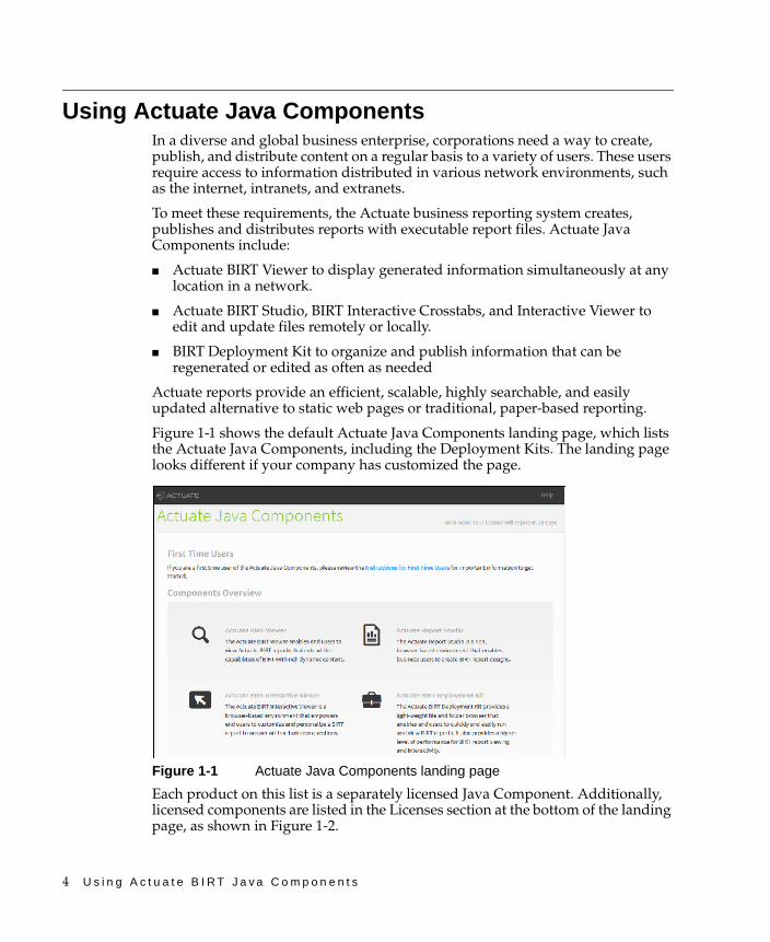
Figure 1-1 shows the default Actuate Java Components landing page, which lists the Actuate Java Components, including the Deployment Kits. The landing page looks different if your company has customized the page.
Figure 1-1 Actuate Java Components landing page
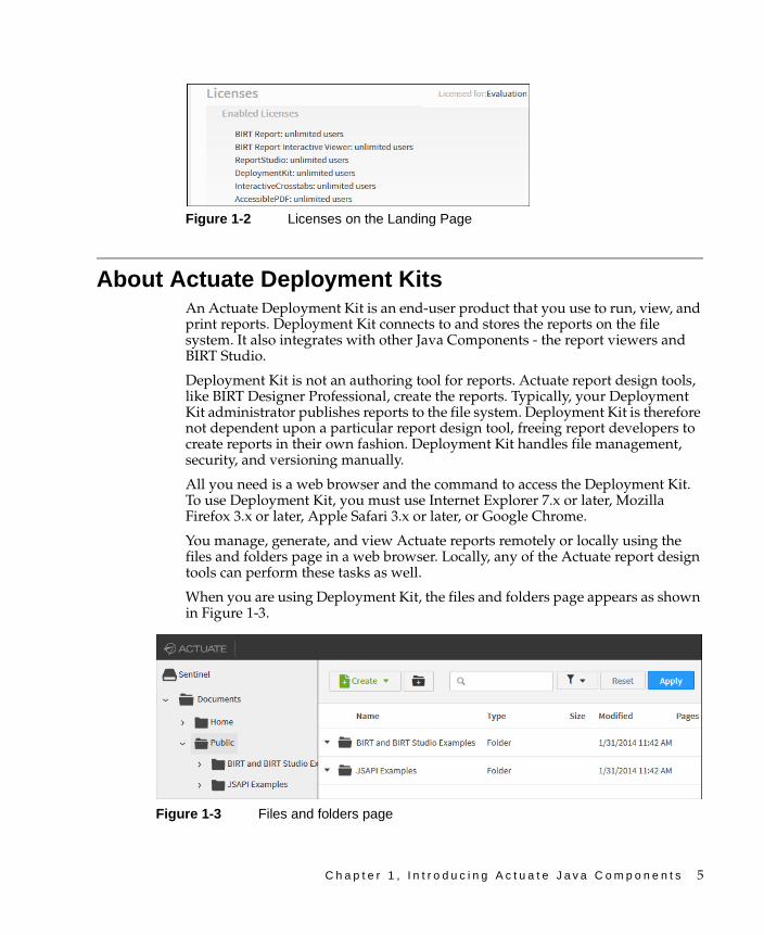
Each product on this list is a separately licensed Java Component. Additionally, licensed components are listed in the Licenses section at the bottom of the landing page, as shown in Figure 1-2.
C h a p t e r 1 , I n t r o d u c i n g A c t u a t e J a v a C o m p o n e n t s 5
Figure 1-2 Licenses on the Landing Page
About Actuate Deployment KitsAn Actuate Deployment Kit is an end-user product that you use to run, view, and print reports. Deployment Kit connects to and stores the reports on the file system. It also integrates with other Java Components - the report viewers and BIRT Studio.
Deployment Kit is not an authoring tool for reports. Actuate report design tools, like BIRT Designer Professional, create the reports. Typically, your Deployment Kit administrator publishes reports to the file system. Deployment Kit is therefore not dependent upon a particular report design tool, freeing report developers to create reports in their own fashion. Deployment Kit handles file management, security, and versioning manually.
All you need is a web browser and the command to access the Deployment Kit. To use Deployment Kit, you must use Internet Explorer 7.x or later, Mozilla Firefox 3.x or later, Apple Safari 3.x or later, or Google Chrome.
You manage, generate, and view Actuate reports remotely or locally using the files and folders page in a web browser. Locally, any of the Actuate report design tools can perform these tasks as well.
When you are using Deployment Kit, the files and folders page appears as shown in Figure 1-3.
Figure 1-3 Files and folders page
6 U s i n g A c t u a t e B I R T J a v a C o m p o n e n t s
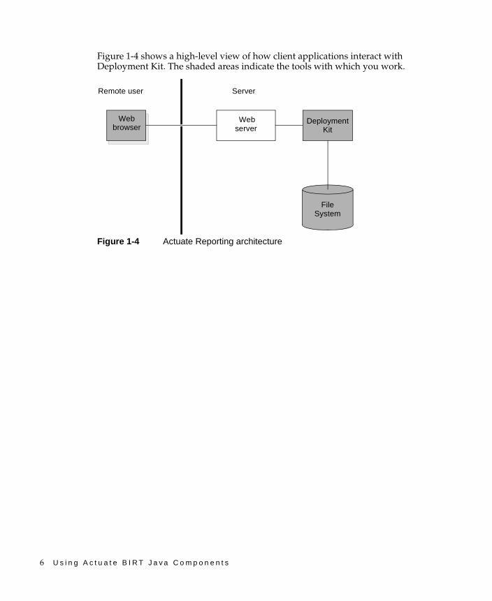
Figure 1-4 shows a high-level view of how client applications interact with Deployment Kit. The shaded areas indicate the tools with which you work.
Figure 1-4 Actuate Reporting architecture
ServerRemote user
Web browser
Web server
Deployment Kit
FileSystem

C h a p t e r 2 , M a n a g i n g f i l e s a n d f o l d e r s 7
C h a p t e r
2Chapter 2Managing files and foldersThis chapter contains the following topics:
■ Getting started with Actuate Java Components
■ Using filters
8 U s i n g A c t u a t e B I R T J a v a C o m p o n e n t s
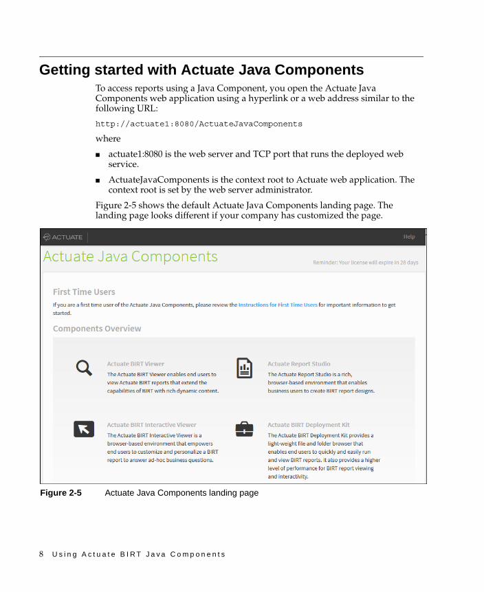
Getting started with Actuate Java ComponentsTo access reports using a Java Component, you open the Actuate Java Components web application using a hyperlink or a web address similar to the following URL:
http://actuate1:8080/ActuateJavaComponents
where
■ actuate1:8080 is the web server and TCP port that runs the deployed web service.
■ ActuateJavaComponents is the context root to Actuate web application. The context root is set by the web server administrator.
Figure 2-5 shows the default Actuate Java Components landing page. The landing page looks different if your company has customized the page.
Figure 2-5 Actuate Java Components landing page
C h a p t e r 2 , M a n a g i n g f i l e s a n d f o l d e r s 9
Each product on this list is a separately licensed Java Component. How you access files depends upon which licenses you have:
■ If you have purchased a Deployment Kit License, you can access reports using a Deployment Kit link.
■ If you have not purchased a license for a Deployment Kit but purchased a license for BIRT Studio, BIRT Interactive Crosstabs, or BIRT Interactive Viewer, you access the reports using a URL for the Documents page. The Documents page has identical functionality to that of the Deployment Kit Documents page.
■ If you have only purchased a license for BIRT Viewer, you do not have access to the Documents page and only view reports for which you have a direct URL.
This manual uses the BIRT Deployment Kit as an example. The Documents page for each product has the same appearance and functionality. The pages for each Deployment Kit have the same appearance and functionality.
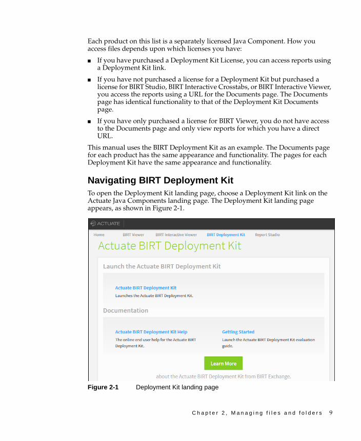
Navigating BIRT Deployment KitTo open the Deployment Kit landing page, choose a Deployment Kit link on the Actuate Java Components landing page. The Deployment Kit landing page appears, as shown in Figure 2-1.
Figure 2-1 Deployment Kit landing page
10 U s i n g A c t u a t e B I R T J a v a C o m p o n e n t s
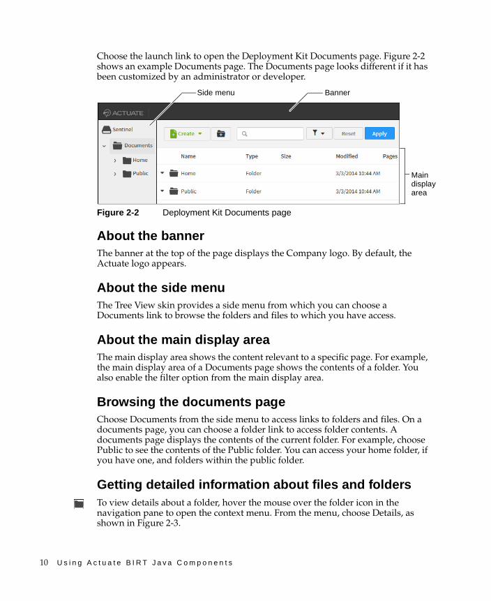
Choose the launch link to open the Deployment Kit Documents page. Figure 2-2 shows an example Documents page. The Documents page looks different if it has been customized by an administrator or developer.
Figure 2-2 Deployment Kit Documents page
About the bannerThe banner at the top of the page displays the Company logo. By default, the Actuate logo appears.
About the side menuThe Tree View skin provides a side menu from which you can choose a Documents link to browse the folders and files to which you have access.
About the main display areaThe main display area shows the content relevant to a specific page. For example, the main display area of a Documents page shows the contents of a folder. You also enable the filter option from the main display area.
Browsing the documents pageChoose Documents from the side menu to access links to folders and files. On a documents page, you can choose a folder link to access folder contents. A documents page displays the contents of the current folder. For example, choose Public to see the contents of the Public folder. You can access your home folder, if you have one, and folders within the public folder.
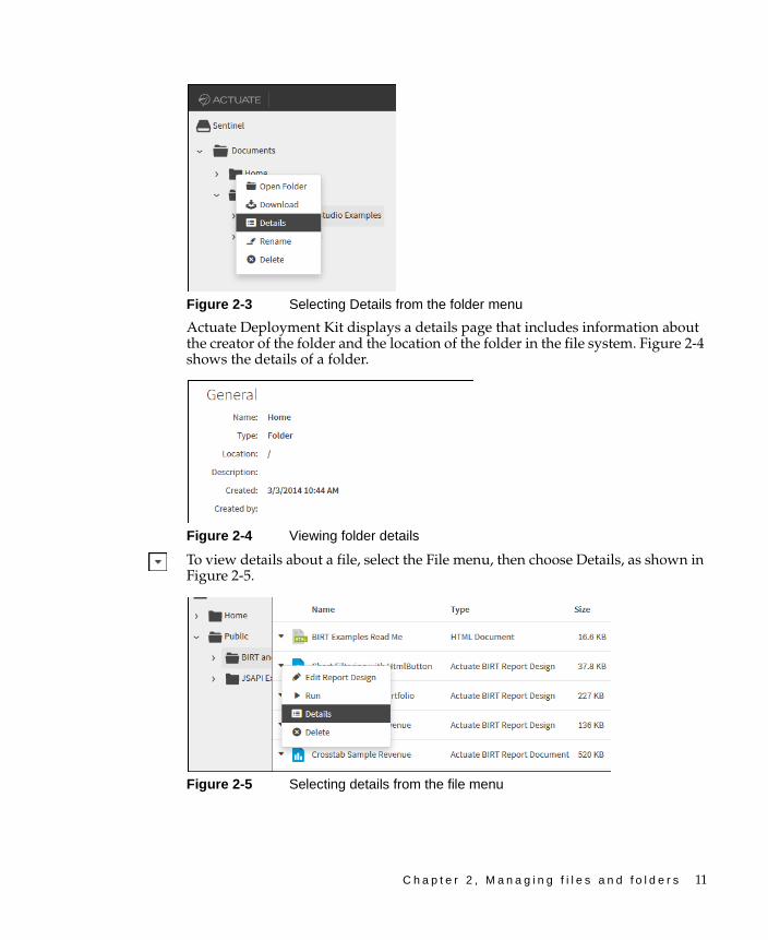
Getting detailed information about files and foldersTo view details about a folder, hover the mouse over the folder icon in the navigation pane to open the context menu. From the menu, choose Details, as shown in Figure 2-3.
Side menu
Main display area
Banner
C h a p t e r 2 , M a n a g i n g f i l e s a n d f o l d e r s 11
Figure 2-3 Selecting Details from the folder menu
Actuate Deployment Kit displays a details page that includes information about the creator of the folder and the location of the folder in the file system. Figure 2-4 shows the details of a folder.
Figure 2-4 Viewing folder details
To view details about a file, select the File menu, then choose Details, as shown in Figure 2-5.
Figure 2-5 Selecting details from the file menu
12 U s i n g A c t u a t e B I R T J a v a C o m p o n e n t s
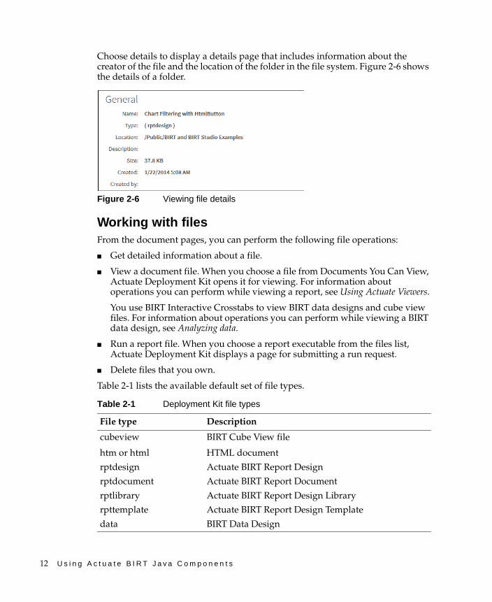
Choose details to display a details page that includes information about the creator of the file and the location of the folder in the file system. Figure 2-6 shows the details of a folder.
Figure 2-6 Viewing file details
Working with filesFrom the document pages, you can perform the following file operations:
■ Get detailed information about a file.
■ View a document file. When you choose a file from Documents You Can View, Actuate Deployment Kit opens it for viewing. For information about operations you can perform while viewing a report, see Using Actuate Viewers.
You use BIRT Interactive Crosstabs to view BIRT data designs and cube view files. For information about operations you can perform while viewing a BIRT data design, see Analyzing data.
■ Run a report file. When you choose a report executable from the files list, Actuate Deployment Kit displays a page for submitting a run request.
■ Delete files that you own.
Table 2-1 lists the available default set of file types.
Table 2-1 Deployment Kit file types
File type Description
cubeview BIRT Cube View file
htm or html HTML document
rptdesign Actuate BIRT Report Design
rptdocument Actuate BIRT Report Document
rptlibrary Actuate BIRT Report Design Library
rpttemplate Actuate BIRT Report Design Template
data BIRT Data Design
C h a p t e r 2 , M a n a g i n g f i l e s a n d f o l d e r s 13
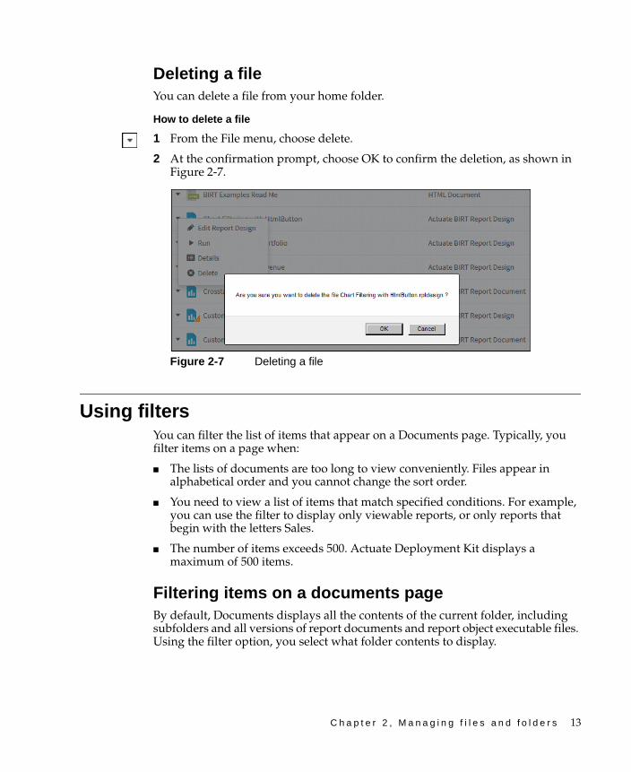
Deleting a fileYou can delete a file from your home folder.
How to delete a file
1 From the File menu, choose delete.
2 At the confirmation prompt, choose OK to confirm the deletion, as shown in Figure 2-7.
Figure 2-7 Deleting a file
Using filtersYou can filter the list of items that appear on a Documents page. Typically, you filter items on a page when:
■ The lists of documents are too long to view conveniently. Files appear in alphabetical order and you cannot change the sort order.
■ You need to view a list of items that match specified conditions. For example, you can use the filter to display only viewable reports, or only reports that begin with the letters Sales.
■ The number of items exceeds 500. Actuate Deployment Kit displays a maximum of 500 items.
Filtering items on a documents pageBy default, Documents displays all the contents of the current folder, including subfolders and all versions of report documents and report object executable files. Using the filter option, you select what folder contents to display.
14 U s i n g A c t u a t e B I R T J a v a C o m p o n e n t s
How to filter items on a documents page
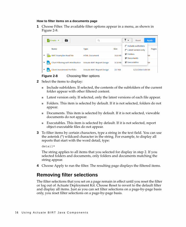
1 Choose Filter. The available filter options appear in a menu, as shown in Figure 2-8.
Figure 2-8 Choosing filter options
2 Select the items to display:
■ Include subfolders. If selected, the contents of the subfolders of the current folder appear with other filtered content.
■ Latest version only. If selected, only the latest versions of each file appear.
■ Folders. This item is selected by default. If it is not selected, folders do not appear.
■ Documents. This item is selected by default. If it is not selected, viewable documents do not appear.
■ Executables. This item is selected by default. If it is not selected, report object executable files do not appear.
3 To filter items by certain characters, type a string in the text field. You can use the asterisk (*) wildcard character in the string. For example, to display all reports that start with the word detail, type:
detail*
The string applies to all items that you selected for display in step 2. If you selected folders and documents, only folders and documents matching the string appear.
4 Choose Apply to run the filter. The resulting page displays the filtered items.
Removing filter selectionsThe filter selections that you set on a page remain in effect until you reset the filter or log out of Actuate Deployment Kit. Choose Reset to revert to the default filter and display all items. Just as you can set filter selections on a page-by-page basis only, you reset filter selections on a page-by-page basis.

C h a p t e r 3 , R u n n i n g j o b s 15
C h a p t e r
3Chapter 3Running jobs
This chapter contains the following topics:
■ Running a job
■ Using parameters
16 U s i n g A c t u a t e B I R T J a v a C o m p o n e n t s
Running a jobYou run a report executable when you want Actuate Deployment Kit to generate a report with the most current data. A report executable file contains compiled code that specifies how the server generates a report and what data it retrieves for the report. A specific run of a report executable or opening of a document file is called a job. You run BIRT Report Design (.rptdesign) files and open BIRT Report Documents (.rptdocument) files using Actuate BIRT Deployment Kit.
When you run a job, Deployment Kit provides some default settings. You change these settings to filter report data by report parameters.
Running a BIRT report job Running a job instructs the server to process a report executable or open a document immediately. When the job successfully finishes, the generated output appears. If the job takes a few minutes to finish, Actuate Deployment Kit displays the completed pages as they become available.
How to run a job
This procedure describes how to run a BIRT report design executable (.rptdesign) file.
1 Navigate to the folder that contains the .rptdesign file.
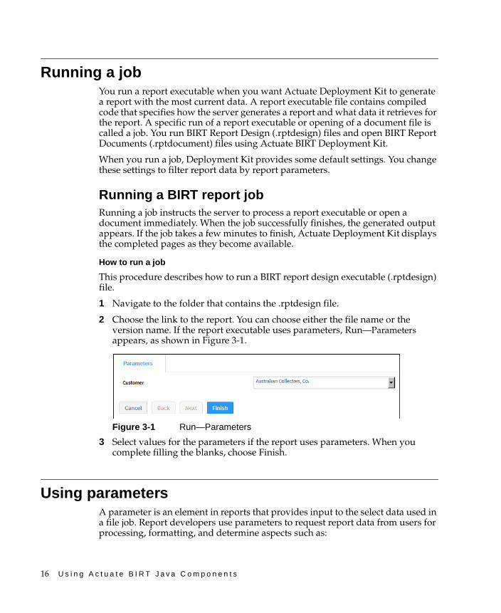
2 Choose the link to the report. You can choose either the file name or the version name. If the report executable uses parameters, Run—Parameters appears, as shown in Figure 3-1.
Figure 3-1 Run—Parameters
3 Select values for the parameters if the report uses parameters. When you complete filling the blanks, choose Finish.
Using parametersA parameter is an element in reports that provides input to the select data used in a file job. Report developers use parameters to request report data from users for processing, formatting, and determine aspects such as:

C h a p t e r 3 , R u n n i n g j o b s 17
■ Which records are retrieved
■ The sorting sequence of the data
■ The output format
If an Actuate file has parameters, the user either sets the parameter values when running the file job, uses the default parameter values, if available, or can use a report parameter file that starts a report and loads the report parameters with predefined values.
Understanding parameter typesThe parameter types are:
■ Single-valueA single-value parameter accepts one value to filter the document data. For example, a report that provides sales information by customer requires the user to select a customer from a list of existing customers.
■ Multiple-valueA multiple-value parameter accepts more than one value to filter the document data. For example, a report that provides sales information of products sold can request the user to select multiple products.
■ OptionalA user can select or group the data presented in a report by typing values or conditions into the optional parameter. If a user does not specify a value for an optional parameter, the document job uses a value chosen by the document designer.
■ RequiredA required parameter must have a value before the document job can run. For example, a report that accesses a database can require a user name and password or require a user to select a city before running a city report. Typically, a document designer supplies a default value for a required parameter.
■ CascadingParameter choices depend on other parameters. For example, a parameter to select from a list of cities is empty until the country is selected first.
■ Dynamic filterA dynamic filter parameter uses an operator and one or more values to retrieve or filter data from a data set. This data appears in the tables, charts, maps, or other presentation formats built into the report.
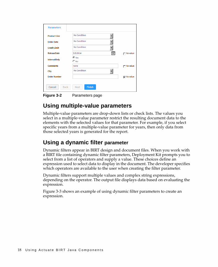
The example in Figure 3-2 shows Parameters prompting input of values for several parameter types.
18 U s i n g A c t u a t e B I R T J a v a C o m p o n e n t s
Figure 3-2 Parameters page
Using multiple-value parameters Multiple-value parameters are drop-down lists or check lists. The values you select in a multiple-value parameter restrict the resulting document data to the elements with the selected values for that parameter. For example, if you select specific years from a multiple-value parameter for years, then only data from those selected years is generated for the report.
Using a dynamic filter parameterDynamic filters appear in BIRT design and document files. When you work with a BIRT file containing dynamic filter parameters, Deployment Kit prompts you to select from a list of operators and supply a value. These choices define an expression used to select data to display in the document. The developer specifies which operators are available to the user when creating the filter parameter.
Dynamic filters support multiple values and complex string expressions, depending on the operator. The output file displays data based on evaluating the expression.
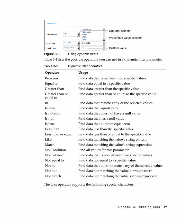
Figure 3-3 shows an example of using dynamic filter parameters to create an expression.
C h a p t e r 3 , R u n n i n g j o b s 19
Figure 3-3 Using dynamic filters
Table 3-1 lists the possible operators you can use in a dynamic filter parameter.
The Like operator supports the following special characters:
Table 3-1 Dynamic filter operators
Operator Usage
Between Find data that is between two specific values
Equal to Find data equal to a specific value
Greater than Find data greater than the specific value
Greater than or equal to
Find data greater than or equal to the specific value
In Find data that matches any of the selected values
Is false Find data that equals zero
Is not null Find data that does not have a null value
Is null Find data that has a null value
Is true Find data that does not equal zero
Less than Find data less than the specific value
Less than or equal Find data less than or equal to the specific value
Like Find data matching the value’s string pattern
Match Find data matching the value’s string expression
No Condition Find all values for this parameter
Not between Find data that is not between two specific values
Not equal to Find data not equal to a specific value
Not in Find data that does not match any of the selected values
Not like Find data not matching the value’s string pattern
Not match Find data not matching the value’s string expression
Custom value
Operator selector
Predefined value selector
20 U s i n g A c t u a t e B I R T J a v a C o m p o n e n t s
■ % matches zero or more characters. For example, %ace% matches any value that contains the string ace, such as Ace Corporation, Facebook, Kennedy Space Center, and MySpace.
■ _ matches exactly one character. For example, t_n matches tan, ten, tin, and ton. It does not match teen or tn.
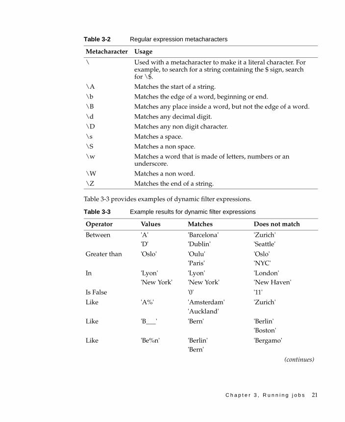
The Match operator is case sensitive and supports special metacharacters that can be combined to form text patterns called regular expressions. Metacharacters can be combined to form complex matches. For example, using ^H.*(Gifts|Collectables)$ to search through a list of company names matches all companies whose name starts with the letter H, has one or more letters after H and includes the word Gifts or Collectables at the end of the name.
If you need to match on a metacharacter itself, a backslash (\) followed by the metacharacter causes the search to interpret the metacharacter as a normal character. For example, if $ is part of the data to be found, it must be entered as \$ because $ is a metacharacter.
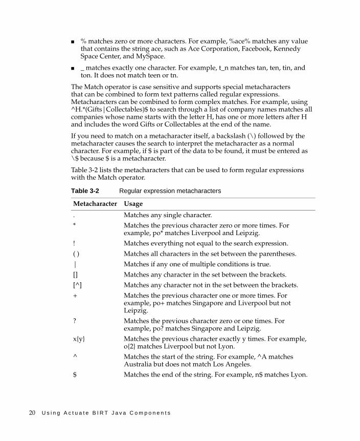
Table 3-2 lists the metacharacters that can be used to form regular expressions with the Match operator.
Table 3-2 Regular expression metacharacters
Metacharacter Usage
. Matches any single character.
* Matches the previous character zero or more times. For example, po* matches Liverpool and Leipzig.
! Matches everything not equal to the search expression.
( ) Matches all characters in the set between the parentheses.
| Matches if any one of multiple conditions is true.
[] Matches any character in the set between the brackets.
[^] Matches any character not in the set between the brackets.
+ Matches the previous character one or more times. For example, po+ matches Singapore and Liverpool but not Leipzig.
? Matches the previous character zero or one times. For example, po? matches Singapore and Leipzig.
x{y} Matches the previous character exactly y times. For example, o{2} matches Liverpool but not Lyon.
^ Matches the start of the string. For example, ^A matches Australia but does not match Los Angeles.
$ Matches the end of the string. For example, n$ matches Lyon.
C h a p t e r 3 , R u n n i n g j o b s 21
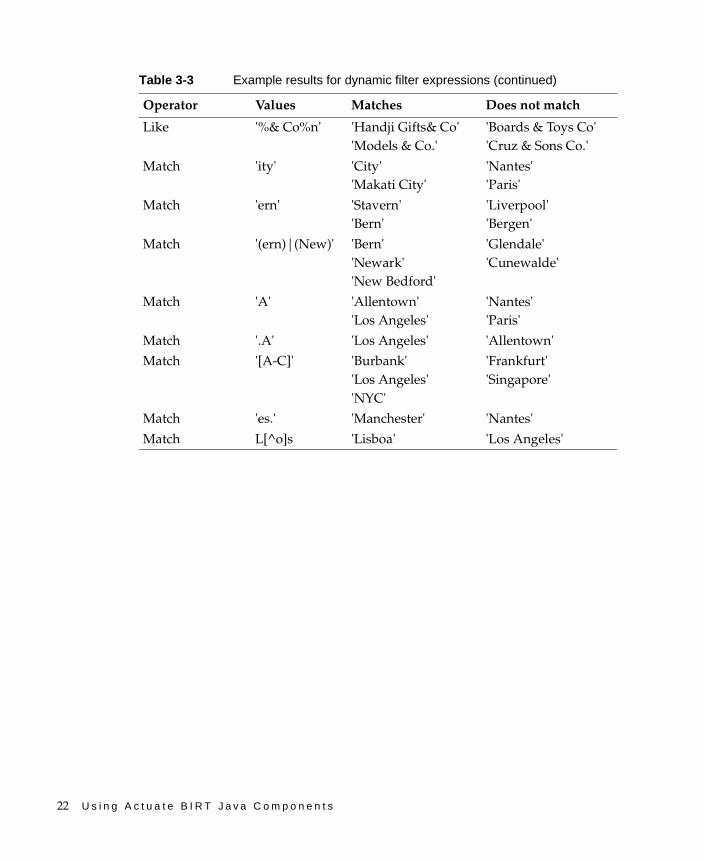
Table 3-3 provides examples of dynamic filter expressions.
\ Used with a metacharacter to make it a literal character. For example, to search for a string containing the $ sign, search for \$.
\A Matches the start of a string.
\b Matches the edge of a word, beginning or end.
\B Matches any place inside a word, but not the edge of a word.
\d Matches any decimal digit.
\D Matches any non digit character.
\s Matches a space.
\S Matches a non space.
\w Matches a word that is made of letters, numbers or an underscore.
\W Matches a non word.
\Z Matches the end of a string.
Table 3-3 Example results for dynamic filter expressions
Operator Values Matches Does not match
Between 'A''D'
'Barcelona''Dublin'
'Zurich''Seattle'
Greater than 'Oslo' 'Oulu''Paris'
'Oslo''NYC'
In 'Lyon''New York'
'Lyon''New York'
'London''New Haven'
Is False '0' '11'
Like 'A%' 'Amsterdam''Auckland'
'Zurich'
Like 'B___' 'Bern' 'Berlin''Boston'
Like 'Be%n' 'Berlin''Bern'
'Bergamo'
(continues)
Table 3-2 Regular expression metacharacters
Metacharacter Usage
22 U s i n g A c t u a t e B I R T J a v a C o m p o n e n t s
Like '%& Co%n' 'Handji Gifts& Co''Models & Co.'
'Boards & Toys Co''Cruz & Sons Co.'
Match 'ity' 'City''Makati City'
'Nantes''Paris'
Match 'ern' 'Stavern''Bern'
'Liverpool''Bergen'
Match '(ern)|(New)' 'Bern''Newark''New Bedford'
'Glendale''Cunewalde'
Match 'A' 'Allentown''Los Angeles'
'Nantes''Paris'
Match '.A' 'Los Angeles' 'Allentown'
Match '[A-C]' 'Burbank''Los Angeles''NYC'
'Frankfurt''Singapore'
Match 'es.' 'Manchester' 'Nantes'
Match L[^o]s 'Lisboa' 'Los Angeles'
Table 3-3 Example results for dynamic filter expressions (continued)
Operator Values Matches Does not match
Part 2Using Actuate Viewers
Part Two2

C h a p t e r 4 , I n t r o d u c i n g A c t u a t e v i e w e r s 25
C h a p t e r
4Chapter 4Introducing
Actuate viewersThis chapter contains the following topics:
■ About Actuate viewers
■ Using Actuate Viewer
■ Using Interactive Viewer
■ Comparing the viewers
26 U s i n g A c t u a t e B I R T J a v a C o m p o n e n t s
About Actuate viewersYou can view BIRT (Business Intelligence Reporting Tools) reports using two web-based viewing environments, Actuate Viewer and Actuate Interactive Viewer. In this document, the term viewers refers to both Actuate Viewer and Interactive Viewer.
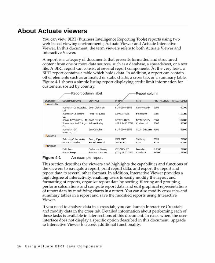
A report is a category of documents that presents formatted and structured content from one or more data sources, such as a database, a spreadsheet, or a text file. A BIRT report can consist of several report components. At the very least, a BIRT report contains a table which holds data. In addition, a report can contain other elements such as animated or static charts, a cross tab, or a summary table. Figure 4-1 shows a simple listing report displaying credit limit information for customers, sorted by country.
Figure 4-1 An example report
This section describes the viewers and highlights the capabilities and functions of the viewers to navigate a report, print report data, and export the report and report data to several other formats. In addition, Interactive Viewer provides a high degree of interactivity, enabling users to easily modify the layout and formatting of reports, organize report data by sorting, filtering and grouping, perform calculations and compute report data, and edit graphical representations of report data by modifying charts in a report. You can also modify cross tabs and summary tables in a report and save the modified reports using Interactive Viewer.
If you need to analyze data in a cross tab, you can launch Interactive Crosstabs and modify data in the cross tab. Detailed information about performing each of these tasks is available in later sections of this document. In cases where the user interface does not display a specific option described in this document, upgrade to Interactive Viewer to access additional functionality.
Report column label Report column
C h a p t e r 4 , I n t r o d u c i n g A c t u a t e v i e w e r s 27
Using Actuate ViewerWhen you generate a report, the primary interface in which you view the report is Actuate Viewer. You can launch Actuate Viewer from any of the following applications:
■ Actuate BIRT Studio
■ Actuate BIRT Designer Professional
■ Actuate Deployment Kit
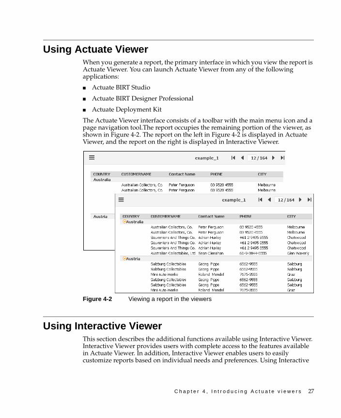
The Actuate Viewer interface consists of a toolbar with the main menu icon and a page navigation tool.The report occupies the remaining portion of the viewer, as shown in Figure 4-2. The report on the left in Figure 4-2 is displayed in Actuate Viewer, and the report on the right is displayed in Interactive Viewer.
Figure 4-2 Viewing a report in the viewers
Using Interactive ViewerThis section describes the additional functions available using Interactive Viewer. Interactive Viewer provides users with complete access to the features available in Actuate Viewer. In addition, Interactive Viewer enables users to easily customize reports based on individual needs and preferences. Using Interactive
28 U s i n g A c t u a t e B I R T J a v a C o m p o n e n t s
Viewer, users can modify the layout of the report, create computed data, move or delete columns, create aggregate data, modify tables displaying summary information, modify charts and graphs, modify data in cross tabs, and rearrange data using simple menu options. You can view and modify a report containing up to 200 pages in Interactive Viewer.
Interactive Viewer operates on a BIRT document file generated from a BIRT design created in BIRT Studio or BIRT Designer Professional. As a result, some properties specified at design time, such as formatting, filters, and so on, cannot be modified using Interactive Viewer. In Interactive Viewer, you can make changes to the BIRT document file, save it as a BIRT design and edit the BIRT design using BIRT Studio and BIRT Designer Professional.
When you purchase the viewers, you have immediate access to Actuate Viewer. To access Interactive Viewer, your system administrator must enable this option on your system, for which you must purchase the Interactive Viewer license.
To view a BIRT report in Interactive Viewer, first view the report using Actuate Viewer. From the main menu, choose Enable Interactivity to launch Interactive Viewer. The menu displays two new options, Undo and Redo, indicating that you are in Interactive Viewer mode. Choose Disable Interactivity from the main menu to return to Actuate Viewer mode.
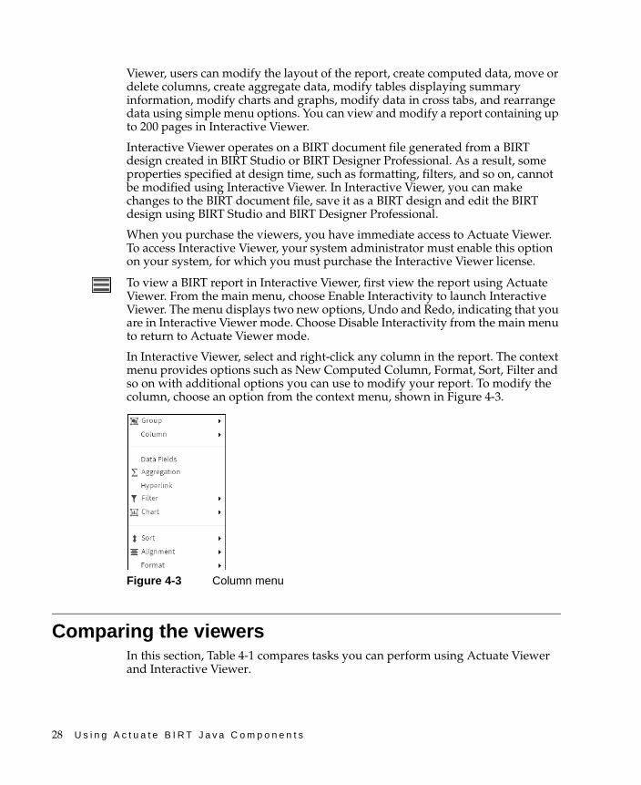
In Interactive Viewer, select and right-click any column in the report. The context menu provides options such as New Computed Column, Format, Sort, Filter and so on with additional options you can use to modify your report. To modify the column, choose an option from the context menu, shown in Figure 4-3.
Figure 4-3 Column menu
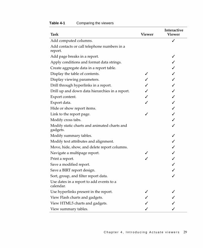
Comparing the viewersIn this section, Table 4-1 compares tasks you can perform using Actuate Viewer and Interactive Viewer.
C h a p t e r 4 , I n t r o d u c i n g A c t u a t e v i e w e r s 29
Table 4-1 Comparing the viewers
Task Viewer Interactive
Viewer
Add computed columns. ✓
Add contacts or call telephone numbers in a report.Add page breaks in a report. ✓
Apply conditions and format data strings. ✓
Create aggregate data in a report table. ✓
Display the table of contents. ✓ ✓
Display viewing parameters. ✓ ✓
Drill through hyperlinks in a report. ✓ ✓
Drill up and down data hierarchies in a report. ✓ ✓
Export content. ✓ ✓
Export data. ✓ ✓
Hide or show report items. ✓
Link to the report page. ✓ ✓
Modify cross tabs. ✓
Modify static charts and animated charts and gadgets.
✓
Modify summary tables. ✓
Modify text attributes and alignment. ✓
Move, hide, show, and delete report columns. ✓
Navigate a multipage report. ✓ ✓
Print a report. ✓ ✓
Save a modified report. ✓
Save a BIRT report design. ✓
Sort, group, and filter report data. ✓
Use dates in a report to add events to a calendar.Use hyperlinks present in the report. ✓ ✓
View Flash charts and gadgets. ✓ ✓
View HTML5 charts and gadgets. ✓ ✓
View summary tables. ✓ ✓

30 U s i n g A c t u a t e B I R T J a v a C o m p o n e n t s
C h a p t e r 5 , E d i t i n g a n d f o r m a t t i n g a r e p o r t 31
C h a p t e r
5Chapter 5Editing and formatting
a reportThis chapter contains the following topics:
■ About editing and formatting options
■ Formatting report data based on conditions
■ Working with data formats
32 U s i n g A c t u a t e B I R T J a v a C o m p o n e n t s
About editing and formatting optionsInteractive Viewer provides you with the flexibility to modify the presentation properties of reports. This section discusses the editing and formatting options available to you.
You can use the context menu in a column in Interactive Viewer to define new font properties and change text alignment for a selected report column, or for the report table. You can also specify these style properties for one column, and copy the style to other columns. You can highlight report data based on certain defined conditions and format data strings depending on the type of data in a column. For example, you can format data strings into currency, telephone number, postal code, date-and-time, or decimal formats.
How to select and format a report element
In a report table, you can format column headers as well as data in the columns. Select and right-click the element, then choose the formatting option from the menu that appears.
Select and right-click a column header and choose a formatting option from the context menu. To select data for formatting, select and right-click the column. A box appears, highlighting the selected element and displaying the menu of available options.
Formatting report data based on conditionsWhen you format data in a selected column, the format applies to all the values. Often, it is useful to change the format of data when a certain condition is true. For example, you can display sales numbers in red if the value is a negative number and in black if the value is a positive number. Conditional formatting is the formatting of data according to defined conditions.
You also can change the format of data in a column according to the values in another column. For example, in a report showing customer names and the number of days each customer’s invoice is past due, you can highlight in blue any customer name that has an invoice past-due value between 60 and 90 days. Then, you can highlight in red and bold any customer name that has an invoice past-due value greater than 90 days.
To apply conditional formatting, you create a rule defining when and how to change the appearance of data. You can apply conditional formats only to data in columns. The rule consists of the condition that must be true, and the text attributes to apply to column entries that satisfy the condition. You can define up to three conditions or rules for a single column and remove or modify conditional formatting for a column.
C h a p t e r 5 , E d i t i n g a n d f o r m a t t i n g a r e p o r t 33
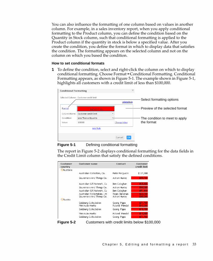
You can also influence the formatting of one column based on values in another column. For example, in a sales inventory report, when you apply conditional formatting to the Product column, you can define the condition based on the Quantity in Stock column, such that conditional formatting is applied to the Product column if the quantity in stock is below a specified value. After you create the condition, you define the format in which to display data that satisfies the condition. The formatting appears on the selected column and not on the column on which you based the condition.
How to set conditional formats
1 To define the condition, select and right-click the column on which to display conditional formatting. Choose Format➛Conditional Formatting. Conditional Formatting appears, as shown in Figure 5-1. The example shown in Figure 5-1, highlights all customers with a credit limit of less than $100,000.
Figure 5-1 Defining conditional formatting
The report in Figure 5-2 displays conditional formatting for the data fields in the Credit Limit column that satisfy the defined conditions.
Figure 5-2 Customers with credit limits below $100,000
The condition to meet to apply the format
Preview of the selected format
Select formatting options
34 U s i n g A c t u a t e B I R T J a v a C o m p o n e n t s
2 In Conditional Formatting, create a rule specifying the following information, then choose OK:
■ The format to apply, such as bold style. Choose Format to select formatting options.
■ The condition that must be true to apply the format, such as Credit Limit Less than or Equal to 100000.
Specifying a conditionThe condition in a conditional formatting rule is an If expression that must evaluate to True. For example:
If the order total is less than 1000If the customer credit limit is between 100000 and 200000If the sales office is TokyoIf the order date is 7/21/2008
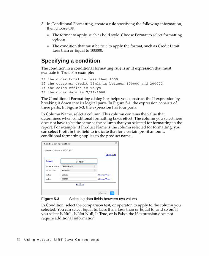
The Conditional Formatting dialog box helps you construct the If expression by breaking it down into its logical parts. In Figure 5-1, the expression consists of three parts. In Figure 5-3, the expression has four parts.
In Column Name, select a column. This column contains the value that determines when conditional formatting takes effect. The column you select here does not have to be the same as the column that you selected for formatting in the report. For example, if Product Name is the column selected for formatting, you can select Profit in this field to indicate that for a certain profit amount, conditional formatting applies to the product name.
Figure 5-3 Selecting data fields between two values
In Condition, select the comparison test, or operator, to apply to the column you selected. You can select Equal to, Less than, Less than or Equal to, and so on. If you select Is Null, Is Not Null, Is True, or Is False, the If expression does not require additional information.
C h a p t e r 5 , E d i t i n g a n d f o r m a t t i n g a r e p o r t 35
If you select an operator that requires a comparison to one or more values, one or more additional fields appear. For example, if you select Less than or Equal to, a third field appears. In this field, type the comparison value. If you select Between or Not Between, a third and fourth field appear. In these fields, type the lower and upper values, respectively, as shown in Figure 5-3.
Comparing to a literal valueThe conditional expression, shown in Figure 5-3 in the previous section, evaluates the Credit Limit column and compares each value to determine if it matches a value between 100000 and 200000. The 100000 and 200000 values are literal values that you type.
Alternatively, you can select a value from the list of values in the Credit Limit column. Selecting from a list of values is useful if the comparison value is a customer name and you do not know the exact customer names, or if the comparison value is a date and you do not know the date format to type. If the comparison value is a date, Interactive Viewer also provides a calendar tool, which you can use to select a date.
How to select a comparison value from a list of values
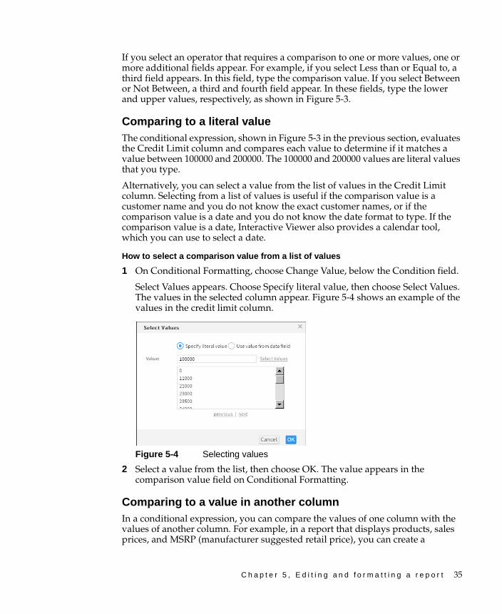
1 On Conditional Formatting, choose Change Value, below the Condition field.
Select Values appears. Choose Specify literal value, then choose Select Values. The values in the selected column appear. Figure 5-4 shows an example of the values in the credit limit column.
Figure 5-4 Selecting values
2 Select a value from the list, then choose OK. The value appears in the comparison value field on Conditional Formatting.
Comparing to a value in another columnIn a conditional expression, you can compare the values of one column with the values of another column. For example, in a report that displays products, sales prices, and MSRP (manufacturer suggested retail price), you can create a
36 U s i n g A c t u a t e B I R T J a v a C o m p o n e n t s
conditional formatting rule that compares the sale price and MSRP of each product, and highlight the names of the products whose sales price is greater than MSRP.
How to compare to a value in another column
1 On Conditional Formatting, choose Change Value, below the Condition field.
2 On Select values, select Use value from data field. A list of columns used in the report appears.
3 Select a column from the list, then choose OK. The column name appears in the comparison value field on Conditional Formatting.
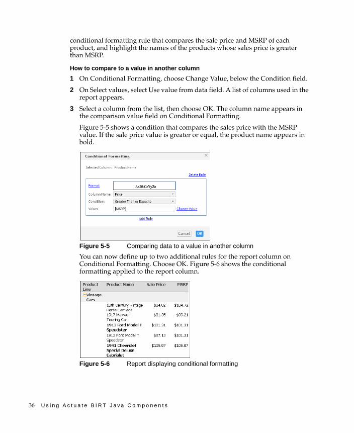
Figure 5-5 shows a condition that compares the sales price with the MSRP value. If the sale price value is greater or equal, the product name appears in bold.
Figure 5-5 Comparing data to a value in another column
You can now define up to two additional rules for the report column on Conditional Formatting. Choose OK. Figure 5-6 shows the conditional formatting applied to the report column.
Figure 5-6 Report displaying conditional formatting
C h a p t e r 5 , E d i t i n g a n d f o r m a t t i n g a r e p o r t 37
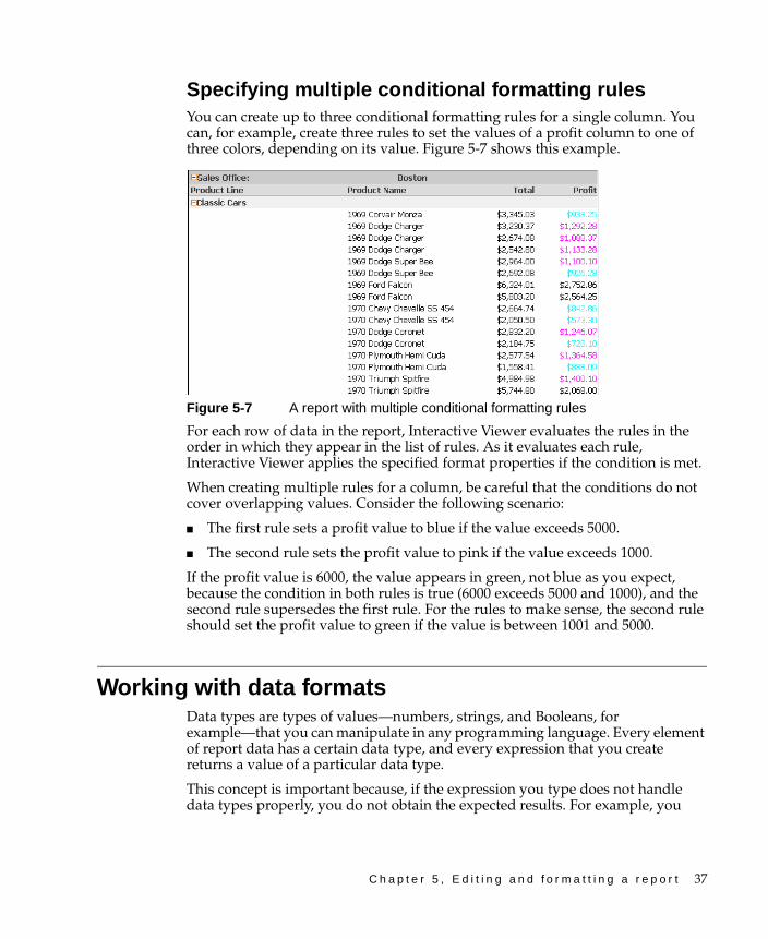
Specifying multiple conditional formatting rulesYou can create up to three conditional formatting rules for a single column. You can, for example, create three rules to set the values of a profit column to one of three colors, depending on its value. Figure 5-7 shows this example.
Figure 5-7 A report with multiple conditional formatting rules
For each row of data in the report, Interactive Viewer evaluates the rules in the order in which they appear in the list of rules. As it evaluates each rule, Interactive Viewer applies the specified format properties if the condition is met.
When creating multiple rules for a column, be careful that the conditions do not cover overlapping values. Consider the following scenario:
■ The first rule sets a profit value to blue if the value exceeds 5000.
■ The second rule sets the profit value to pink if the value exceeds 1000.
If the profit value is 6000, the value appears in green, not blue as you expect, because the condition in both rules is true (6000 exceeds 5000 and 1000), and the second rule supersedes the first rule. For the rules to make sense, the second rule should set the profit value to green if the value is between 1001 and 5000.
Working with data formatsData types are types of values—numbers, strings, and Booleans, for example—that you can manipulate in any programming language. Every element of report data has a certain data type, and every expression that you create returns a value of a particular data type.
This concept is important because, if the expression you type does not handle data types properly, you do not obtain the expected results. For example, you
38 U s i n g A c t u a t e B I R T J a v a C o m p o n e n t s
cannot perform mathematical calculations on numbers if they are of string type, and you cannot convert values in a date field to uppercase characters.
If you type an expression to manipulate a data field, make sure you verify its type, particularly if the data consists of numbers. Numbers can be of string type or numeric type. For example, databases typically store postal codes and telephone numbers as strings. Item quantities or prices are always of numeric type so that you can manipulate the data mathematically. IDs such as customer IDs, or order IDs are usually of numeric type so that the application can store them in numeric order, such as 1, 2, 3, 10, 11, rather than in alphanumeric order, such as 1, 10, 11, 2, 3.
To view the data type of a column, select the column and choose Format➛Format Data from the context menu. The name of the dialog box that appears tells you the type of data in the column. For example, if you select the credit limit column, the dialog box that appears is called Number column format.
When working with multiple columns containing the same data type, you can use Interactive Viewer to specify a format for the data in one column, and copy the format to other columns. This section also explains how to copy formatting properties.
About standard data formatsInteractive Viewer provides common data formats to change how numbers appear. You can, for example, display numbers with or without decimal values, in scientific notation, as a percentage, or as currency with the appropriate symbol. Sometimes, even though a column displays numbers, the data can have a string data type. Postal codes, for example, are frequently stored as string data. Numeric formats do not apply to numbers of string type. When you work with merged columns, select each column from the drop-down list of columns in the merged column, and define a new format each time, based on the column’s data type.
Applying a standard number formatTable 5-1 shows the standard number formats that Interactive Viewer supports. The examples in the table reflect the English (United States) locale. If you work in a different locale, the data displays differently. For example, a number that appears as 1352.45 in the English (United States) locale appears as 1352,45 in the French (France) locale.
Table 5-1 Standard number formats
Format Example of data display
General Number 6066.45 or 6066.5 or 6067, depending on the original value. This format displays up to two decimal places. Whole numbers and numbers with one or two decimal places appear in their original format.
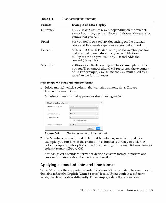
C h a p t e r 5 , E d i t i n g a n d f o r m a t t i n g a r e p o r t 39
How to apply a standard number format
1 Select and right-click a column that contains numeric data. Choose Format➛Format Data.
Number column format appears, as shown in Figure 5-8.
Figure 5-8 Setting number column format
2 On Number column format, in Format Number as, select a format. For example, you can format the credit limit column as currency in dollars ($). Select the appropriate options from the remaining drop-down lists on Number column format. Choose OK.
You can select a standard format or define a custom format. Standard and custom formats are described in the next sections.
Applying a standard date-and-time formatTable 5-2 shows the supported standard date-and-time formats. The examples in the table reflect the English (United States) locale. If you work in a different locale, the date displays differently. For example, a date that appears as
Currency $6,067.45 or ¥6067 or 6067€, depending on the symbol, symbol position, decimal place, and thousands separator values that you set.
Fixed 6067 or 6067.5 or 6,067.45, depending on the decimal place and thousands separator values that you set.
Percent 45% or 45.8% or %45, depending on the symbol position and decimal place values that you set. This format multiplies the original value by 100 and adds the percent (%) symbol.
Scientific 2E04 or 2.67E04, depending on the decimal place value you set. The number after the E represents the exponent of 10. For example, 2.67E04 means 2.67 multiplied by 10 raised to the fourth power.
Table 5-1 Standard number formats
Format Example of data display
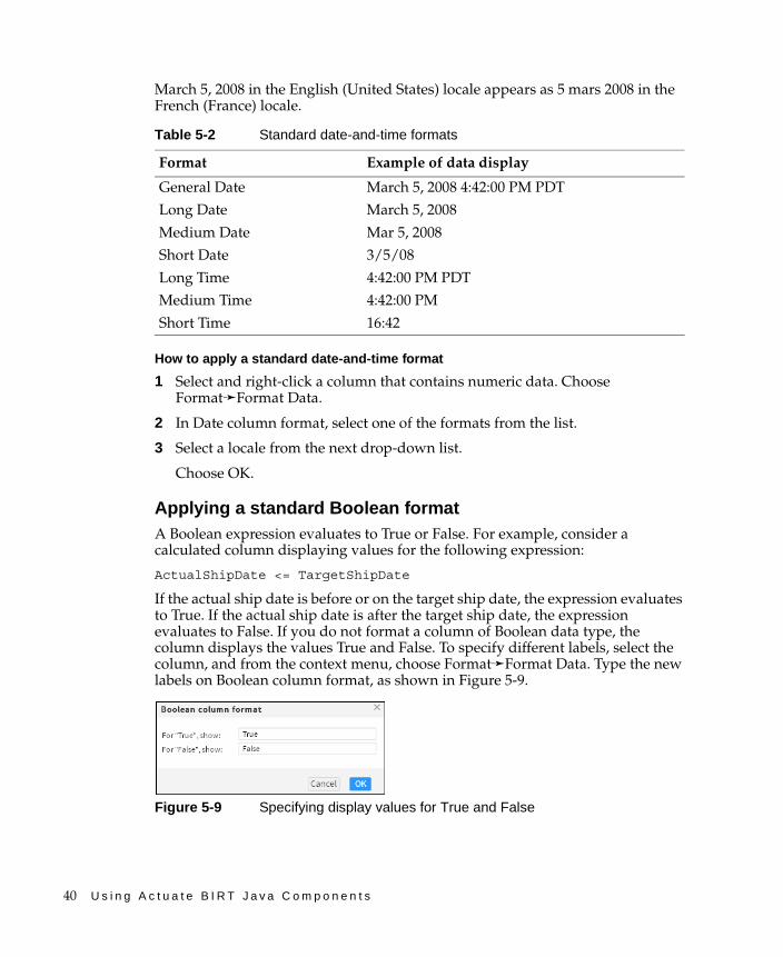
40 U s i n g A c t u a t e B I R T J a v a C o m p o n e n t s
March 5, 2008 in the English (United States) locale appears as 5 mars 2008 in the French (France) locale.
How to apply a standard date-and-time format
1 Select and right-click a column that contains numeric data. Choose Format➛Format Data.
2 In Date column format, select one of the formats from the list.
3 Select a locale from the next drop-down list.
Choose OK.
Applying a standard Boolean formatA Boolean expression evaluates to True or False. For example, consider a calculated column displaying values for the following expression:
ActualShipDate <= TargetShipDate
If the actual ship date is before or on the target ship date, the expression evaluates to True. If the actual ship date is after the target ship date, the expression evaluates to False. If you do not format a column of Boolean data type, the column displays the values True and False. To specify different labels, select the column, and from the context menu, choose Format➛Format Data. Type the new labels on Boolean column format, as shown in Figure 5-9.
Figure 5-9 Specifying display values for True and False
Table 5-2 Standard date-and-time formats
Format Example of data display
General Date March 5, 2008 4:42:00 PM PDT
Long Date March 5, 2008
Medium Date Mar 5, 2008
Short Date 3/5/08
Long Time 4:42:00 PM PDT
Medium Time 4:42:00 PM
Short Time 16:42
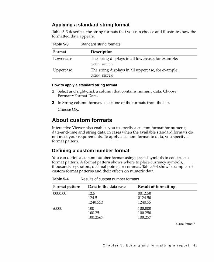
C h a p t e r 5 , E d i t i n g a n d f o r m a t t i n g a r e p o r t 41
Applying a standard string formatTable 5-3 describes the string formats that you can choose and illustrates how the formatted data appears.
How to apply a standard string format
1 Select and right-click a column that contains numeric data. Choose Format➛Format Data.
2 In String column format, select one of the formats from the list.
Choose OK.
About custom formatsInteractive Viewer also enables you to specify a custom format for numeric, date-and-time and string data, in cases when the available standard formats do not meet your requirements. To apply a custom format to data, you specify a format pattern.
Defining a custom number formatYou can define a custom number format using special symbols to construct a format pattern. A format pattern shows where to place currency symbols, thousands separators, decimal points, or commas. Table 5-4 shows examples of custom format patterns and their effects on numeric data.
Table 5-3 Standard string formats
Format Description
Lowercase The string displays in all lowercase, for example:john smith
Uppercase The string displays in all uppercase, for example:JOHN SMITH
Table 5-4 Results of custom number formats
Format pattern Data in the database Result of formatting
0000.00 12.5124.51240.553
0012.500124.501240.55
#.000 100100.25100.2567
100.000100.250100.257
(continues)

42 U s i n g A c t u a t e B I R T J a v a C o m p o n e n t s
Defining a custom date-and-time formatYou can define a custom date-and-time format using special symbols, shown in Table 5-5, to construct a format pattern. Use custom date formatting only for reports viewed in a single locale. Custom formats always display dates in the format you set, which can be inappropriate in other locales. For example, if you use the format MM-dd-yy, the date January 10, 2006 always appears as 01-10-06, regardless of the locale in which you view the report. For locales that customarily display dates in date-month-year format, Interactive Viewer interprets the date 01-10-06 as October 1, 2006.
$#,### 2000.0020000.00
$2,000$20,000
ID # 15 ID 15
Table 5-5 Symbols for defining custom date-and-time formats
Symbol Description Example
yy Short year 08
yyyy Long year 2008
MM Month as a number 07
MMM Short month name Jul
MMMM Full month name July
d Day in month 10
W Week in month 2
w Week in year 28
DD Day in year 192
E Short day of week Thu
EEEE Long day of week Thursday
H Hour in day (0 - 23) 0
k Hour in day (1 - 24) 24
K Hour in AM/PM (0 - 11) 0
h Hour in AM/PM (1 - 12) 12
a AM/PM 12:00:00AM
mm Minutes 30
ss Seconds 55
Table 5-4 Results of custom number formats (continued)
Format pattern Data in the database Result of formatting
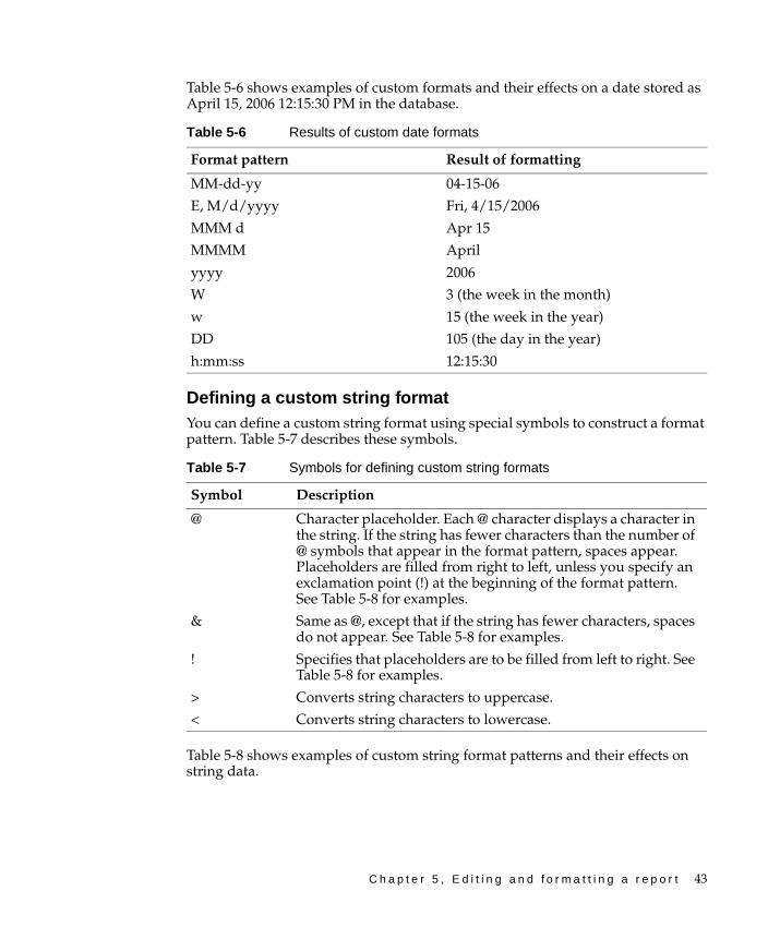
C h a p t e r 5 , E d i t i n g a n d f o r m a t t i n g a r e p o r t 43
Table 5-6 shows examples of custom formats and their effects on a date stored as April 15, 2006 12:15:30 PM in the database.
Defining a custom string formatYou can define a custom string format using special symbols to construct a format pattern. Table 5-7 describes these symbols.
Table 5-8 shows examples of custom string format patterns and their effects on string data.
Table 5-6 Results of custom date formats
Format pattern Result of formatting
MM-dd-yy 04-15-06
E, M/d/yyyy Fri, 4/15/2006
MMM d Apr 15
MMMM April
yyyy 2006
W 3 (the week in the month)
w 15 (the week in the year)
DD 105 (the day in the year)
h:mm:ss 12:15:30
Table 5-7 Symbols for defining custom string formats
Symbol Description
@ Character placeholder. Each @ character displays a character in the string. If the string has fewer characters than the number of @ symbols that appear in the format pattern, spaces appear. Placeholders are filled from right to left, unless you specify an exclamation point (!) at the beginning of the format pattern. See Table 5-8 for examples.
& Same as @, except that if the string has fewer characters, spaces do not appear. See Table 5-8 for examples.
! Specifies that placeholders are to be filled from left to right. See Table 5-8 for examples.
> Converts string characters to uppercase.
< Converts string characters to lowercase.
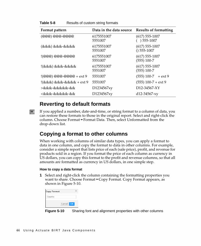
44 U s i n g A c t u a t e B I R T J a v a C o m p o n e n t s
Reverting to default formatsIf you applied a number, date-and-time, or string format to a column of data, you can restore these formats to those in the original report. Select and right-click the column. Choose Format➛Format Data. Then, select Unformatted from the drop-down list.
Copying a format to other columnsWhen working with columns of similar data types, you can apply a format to data in one column, and copy the format to data in other columns. For example, consider a simple report that lists price of each (sale price), profit, and revenue for products sold in a region. If you format the price of each column as currency in US dollars, you can copy this format to the profit and revenue columns, so that all amounts are formatted as currency in US dollars, in one simple step.
How to copy a data format
1 Select and right-click the column containing the formatting properties you want to share. Choose Format➛Copy Format. Copy Format appears, as shown in Figure 5-10.
Figure 5-10 Sharing font and alignment properties with other columns
Table 5-8 Results of custom string formats
Format pattern Data in the data source Results of formatting
(@@@) @@@-@@@@ 61755510075551007
(617) 555-1007( ) 555-1007
(&&&) &&&-&&&& 61755510075551007
(617) 555-1007() 555-1007
!(@@@) @@@-@@@@ 61755510075551007
(617) 555-1007(555) 100-7
!(&&&) &&&-&&&& 61755510075551007
(617) 555-1007(555) 100-7
!(@@@) @@@-@@@@ + ext 9 5551007 (555) 100-7 + ext 9
!(&&&) &&&-&&&& + ext 9 5551007 (555) 100-7 + ext 9
>&&&-&&&&&-&& D1234567xy D12-34567-XY
<&&&-&&&&&-&& D1234567xy d12-34567-xy
C h a p t e r 5 , E d i t i n g a n d f o r m a t t i n g a r e p o r t 45
2 Select the column to which you want to copy the current formatting properties. To select multiple columns, press Ctrl, then select each column.
Choose OK. The report displays the copied formatting properties in the specified columns.

46 U s i n g A c t u a t e B I R T J a v a C o m p o n e n t s

C h a p t e r 6 , E x p o r t i n g r e p o r t d a t a a n d c o n t e n t 47
C h a p t e r
6Chapter 6Exporting report data
and contentThis chapter contains the following topics:
■ About exporting options
■ Exporting content
■ Exporting report data
48 U s i n g A c t u a t e B I R T J a v a C o m p o n e n t s
About exporting optionsThe viewers enable you to export report data, report content, and elements such as charts, cross tabs, or summary tables, to various formats. You can export data to several flat file formats that can be read by Excel. In addition, the viewers and Interactive Crosstabs provide various emitters to enable you to export content in a report table and other report elements to formats such as Excel, Word, PowerPoint, PostScript, and PDF.
When you export content or report elements to other formats, each emitter such as the PDF emitter or the Excel emitter provides several options that you can select to maintain the existing properties of the exported content, enabling users to easily perform additional analysis on the exported output. For example, when you export an element such as a cross tab to Excel, the Excel emitter supports exporting the content as a pivot table. This feature is specifically useful for sharing content with users without access to the viewers, who can still analyze the output in Excel. You can also export an existing Flash chart to PDF format. The PDF emitter embeds the chart in the output file, retaining existing animation properties. You can modify the output file, based on the options available in that application. This section discusses the exporting options available when exporting report data or report content.
Exporting contentYou can export an entire report, as well as each individual report element, such as a chart, summary table, or cross tab, to several different formats. Exporting content to one of these formats creates a file that can be used by other applications in addition to viewers.
Using viewers and Interactive Crosstabs, you can export report content to the following file formats:
■ Microsoft Excel (.xls and .xlsx)
■ PDF (.pdf)
■ PostScript (.ps)
■ Microsoft Word (.doc and .docx)
■ Microsoft PowerPoint (.ppt and .pptx)
■ Extensible HTML (.xhtml)
Table 6-1 describes the exporting options available when exporting to each output format.
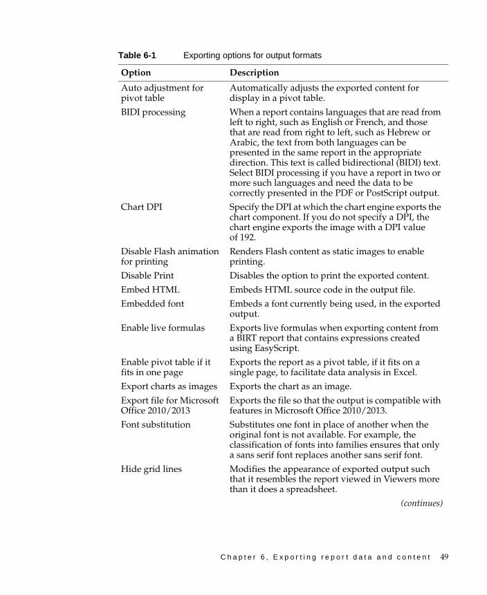
C h a p t e r 6 , E x p o r t i n g r e p o r t d a t a a n d c o n t e n t 49
Table 6-1 Exporting options for output formats
Option Description
Auto adjustment for pivot table
Automatically adjusts the exported content for display in a pivot table.
BIDI processing When a report contains languages that are read from left to right, such as English or French, and those that are read from right to left, such as Hebrew or Arabic, the text from both languages can be presented in the same report in the appropriate direction. This text is called bidirectional (BIDI) text. Select BIDI processing if you have a report in two or more such languages and need the data to be correctly presented in the PDF or PostScript output.
Chart DPI Specify the DPI at which the chart engine exports the chart component. If you do not specify a DPI, the chart engine exports the image with a DPI value of 192.
Disable Flash animation for printing
Renders Flash content as static images to enable printing.
Disable Print Disables the option to print the exported content.
Embed HTML Embeds HTML source code in the output file.
Embedded font Embeds a font currently being used, in the exported output.
Enable live formulas Exports live formulas when exporting content from a BIRT report that contains expressions created using EasyScript.
Enable pivot table if it fits in one page
Exports the report as a pivot table, if it fits on a single page, to facilitate data analysis in Excel.
Export charts as images Exports the chart as an image.
Export file for Microsoft Office 2010/2013
Exports the file so that the output is compatible with features in Microsoft Office 2010/2013.
Font substitution Substitutes one font in place of another when the original font is not available. For example, the classification of fonts into families ensures that only a sans serif font replaces another sans serif font.
Hide grid lines Modifies the appearance of exported output such that it resembles the report viewed in Viewers more than it does a spreadsheet.
(continues)
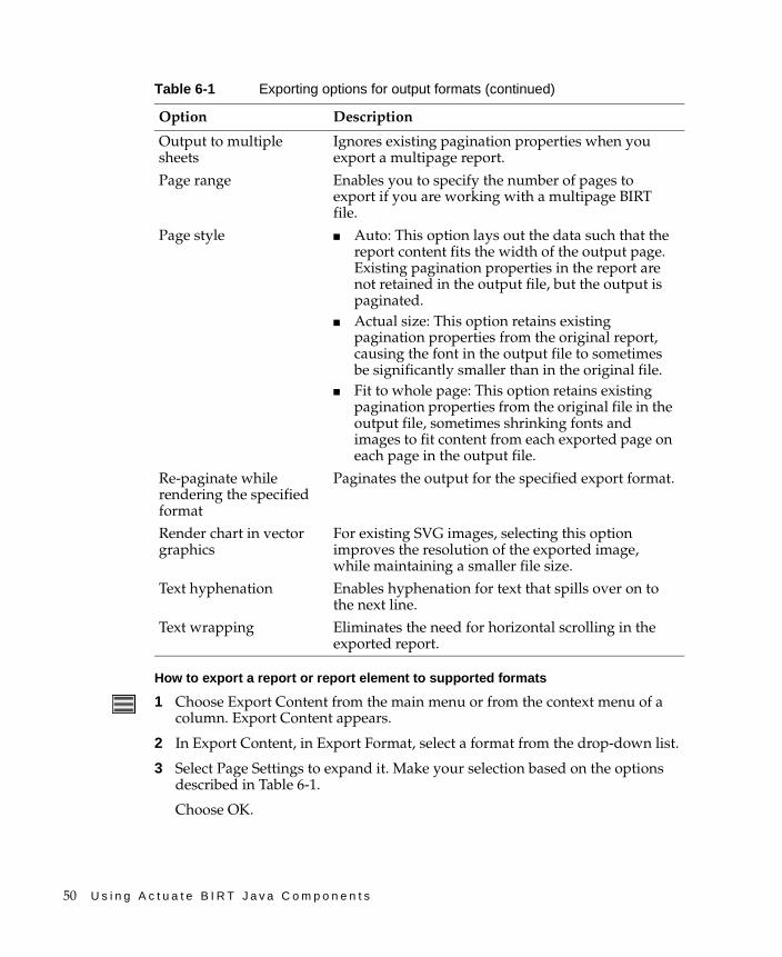
50 U s i n g A c t u a t e B I R T J a v a C o m p o n e n t s
How to export a report or report element to supported formats
1 Choose Export Content from the main menu or from the context menu of a column. Export Content appears.
2 In Export Content, in Export Format, select a format from the drop-down list.
3 Select Page Settings to expand it. Make your selection based on the options described in Table 6-1.
Choose OK.
Output to multiple sheets
Ignores existing pagination properties when you export a multipage report.
Page range Enables you to specify the number of pages to export if you are working with a multipage BIRT file.
Page style ■ Auto: This option lays out the data such that the report content fits the width of the output page. Existing pagination properties in the report are not retained in the output file, but the output is paginated.
■ Actual size: This option retains existing pagination properties from the original report, causing the font in the output file to sometimes be significantly smaller than in the original file.
■ Fit to whole page: This option retains existing pagination properties from the original file in the output file, sometimes shrinking fonts and images to fit content from each exported page on each page in the output file.
Re-paginate while rendering the specified format
Paginates the output for the specified export format.
Render chart in vector graphics
For existing SVG images, selecting this option improves the resolution of the exported image, while maintaining a smaller file size.
Text hyphenation Enables hyphenation for text that spills over on to the next line.
Text wrapping Eliminates the need for horizontal scrolling in the exported report.
Table 6-1 Exporting options for output formats (continued)
Option Description
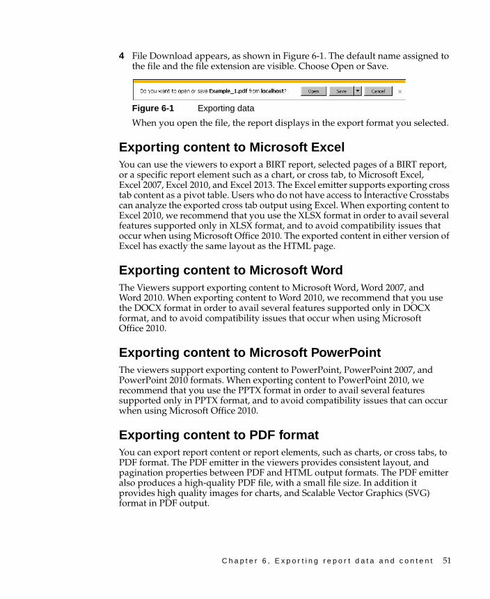
C h a p t e r 6 , E x p o r t i n g r e p o r t d a t a a n d c o n t e n t 51
4 File Download appears, as shown in Figure 6-1. The default name assigned to the file and the file extension are visible. Choose Open or Save.
Figure 6-1 Exporting data
When you open the file, the report displays in the export format you selected.
Exporting content to Microsoft ExcelYou can use the viewers to export a BIRT report, selected pages of a BIRT report, or a specific report element such as a chart, or cross tab, to Microsoft Excel, Excel 2007, Excel 2010, and Excel 2013. The Excel emitter supports exporting cross tab content as a pivot table. Users who do not have access to Interactive Crosstabs can analyze the exported cross tab output using Excel. When exporting content to Excel 2010, we recommend that you use the XLSX format in order to avail several features supported only in XLSX format, and to avoid compatibility issues that occur when using Microsoft Office 2010. The exported content in either version of Excel has exactly the same layout as the HTML page.
Exporting content to Microsoft WordThe Viewers support exporting content to Microsoft Word, Word 2007, and Word 2010. When exporting content to Word 2010, we recommend that you use the DOCX format in order to avail several features supported only in DOCX format, and to avoid compatibility issues that occur when using Microsoft Office 2010.
Exporting content to Microsoft PowerPointThe viewers support exporting content to PowerPoint, PowerPoint 2007, and PowerPoint 2010 formats. When exporting content to PowerPoint 2010, we recommend that you use the PPTX format in order to avail several features supported only in PPTX format, and to avoid compatibility issues that can occur when using Microsoft Office 2010.
Exporting content to PDF formatYou can export report content or report elements, such as charts, or cross tabs, to PDF format. The PDF emitter in the viewers provides consistent layout, and pagination properties between PDF and HTML output formats. The PDF emitter also produces a high-quality PDF file, with a small file size. In addition it provides high quality images for charts, and Scalable Vector Graphics (SVG) format in PDF output.
52 U s i n g A c t u a t e B I R T J a v a C o m p o n e n t s
You can also export Flash charts to PDF format. When you export Flash charts to PDF format, the viewers support embedding the exported element in the PDF file, enabling you to easily interact with the Flash elements. Flash charts retain their animation properties when exported to PDF format.
When you print an exported Flash chart, the embedded file in the PDF document, must first be viewed in order for it to appear on the printed page. In a multipage report with Flash content on several pages, view each page, so that the embedded Flash elements load, and then print the required pages for the Flash content to be visible in the printed output. If you do not view the pages before printing the file, the Flash content is not visible in the printed output, for pages that were not viewed.
Exporting content to PostScript formatWhen you export content to PostScript format, the PostScript emitter displays the content in the output file, almost exactly the same way as it will appear when printed.
Exporting content to Extensible HTML formatExtensible HTML (XHTML) is the next generation of HTML, compliant with XML (Extensible Markup Language) standards. The XHTML emitter is specifically useful when users need to provide accessibility options for the exported content. XHTML (Extensible Hypertext Markup Language) format enables users to access the content from a wide range of applications, other than a desktop or browser, and is extremely easy to update and maintain.
Exporting report dataYou export report data to extract some or all of the data from a report, to use the data in another document or format. For example, you can export customer sales data from a previous quarter, then use the numbers in a spreadsheet to create a forecast for an upcoming quarter. Data displayed in a table is a result set from the report table’s data source. Actuate Viewers enable you to export these result sets in the flat-file formats described in this section.
The viewers support the ability to export report data as a comma-separated values (.csv) file, a pipe-separated values (.psv) file, a tab-separated values (.tsv) file, or a semicolon-separated values (.ssv) file. These files store data in a flat file format, which Excel can read. The difference between these formats is the character used as the data delimiter, which can be a comma, pipe, tab, or semicolon. You choose a format to export report data based on the requirements of the application to which you export the data, and the purpose for which you plan to use the exported data.
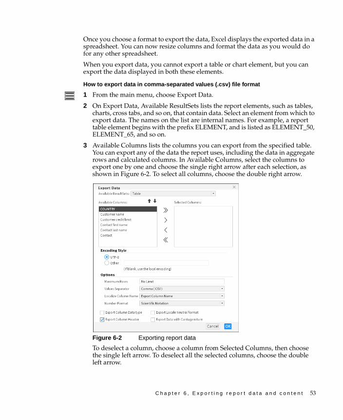
C h a p t e r 6 , E x p o r t i n g r e p o r t d a t a a n d c o n t e n t 53
Once you choose a format to export the data, Excel displays the exported data in a spreadsheet. You can now resize columns and format the data as you would do for any other spreadsheet.
When you export data, you cannot export a table or chart element, but you can export the data displayed in both these elements.
How to export data in comma-separated values (.csv) file format
1 From the main menu, choose Export Data.
2 On Export Data, Available ResultSets lists the report elements, such as tables, charts, cross tabs, and so on, that contain data. Select an element from which to export data. The names on the list are internal names. For example, a report table element begins with the prefix ELEMENT, and is listed as ELEMENT_50, ELEMENT_65, and so on.
3 Available Columns lists the columns you can export from the specified table. You can export any of the data the report uses, including the data in aggregate rows and calculated columns. In Available Columns, select the columns to export one by one and choose the single right arrow after each selection, as shown in Figure 6-2. To select all columns, choose the double right arrow.
Figure 6-2 Exporting report data
To deselect a column, choose a column from Selected Columns, then choose the single left arrow. To deselect all the selected columns, choose the double left arrow.
54 U s i n g A c t u a t e B I R T J a v a C o m p o n e n t s
4 In Encoding Style, select UTF-8, or specify a style in Other. If you do not specify a style, Actuate Viewer uses the local encoding style.
5 In Miscellaneous, specify the following information:
■ In Maximum Rows, type the maximum number of data rows to export. To export all the data rows in the report, accept the default value of No Limit.
■ In Values Separator, choose the Comma (CSV) delimiter.
■ In Localize Column Name, select an option from the following:
❏ Select Export Column Name to export the column name specified in the data source.
❏ Select Export Column Display Name to export the column name specified in the report design.
■ In Number format, do one of the following:
❏ Choose Scientific Notation.
❏ Choose Unformatted.
6 You can select the following additional options to export column data type, export the data in locale neutral format, and export the column header.
■ When you export report data to a flat file format, such as comma-separated values (.csv) format, tab-separated values (.tsv) format, pipe-separated values (.psv) format, or semicolon-separated values format, select Export Column Data Type to include the data type information in the flat file. In the following example, the second line identifies the type of data in the file:
FirstName, LastName, AccountID STRING, STRING, INT "Doe", Jane", 1234 …
■ When you export report data that contains date-and-time values, format these values according to the syntax in the current locale, by default. If no locale is configured, then the viewers use the US locale as the default. For example, if you export the date 01/10/2009 in the original format, it can be interpreted as January 10, 2009 or October 1, 2009, depending on whether the locale is US or France. On Export Data, select Export Locale Neutral Format to export report data without considering locale information, so that the date is interpreted correctly in every locale.
■ When you select Export Column Header, viewers export the column header in addition to the data in the column. The spreadsheet displays each exported column below the corresponding column header.
■ When you select Export Data With Carriage Return, viewers export the data using a Carriage Return (CR) character for each line break.
Choose OK.
C h a p t e r 6 , E x p o r t i n g r e p o r t d a t a a n d c o n t e n t 55
7 On File Download, the default name and the file extension of the spreadsheet file appear.
Choose Save.
8 On Save As, complete the following tasks:
1 In Save in, navigate to the folder in which you want to save the file.
2 In File name, change the name of the file. Choose Save. The comma-separated values (.csv) file appears in the new location.
When you open the file, the output data appears as an editable Microsoft Excel worksheet. You can expand the columns to view all the data.
Use the same process to export data to pipe-separated values (.psv) files, tab-separated values (.tsv) files, and semicolon-separated values (.ssv) files.

56 U s i n g A c t u a t e B I R T J a v a C o m p o n e n t s
C h a p t e r 7 , O r g a n i z i n g a n d m o d i f y i n g d a t a 57
C h a p t e r
7Chapter 7Organizing and modifying
dataThis chapter contains the following topics:
■ About organizing and modifying data
■ Managing a column
■ Sorting data in a column
■ Organizing data in groups
■ Specifying page breaks
■ Inserting a computed column
■ Aggregating data
■ Hiding and displaying report elements
■ Filtering data
■ Working with merged columns
■ Working with summary tables
58 U s i n g A c t u a t e B I R T J a v a C o m p o n e n t s
About organizing and modifying dataInteractive Viewer enables you to organize report data in several ways. You can change the width of columns, and move and remove columns to improve presentation or change the order of data in a report. You can sort data in a column in ascending or descending order, organize data columns into groups, and create computed columns. You can create aggregate data such as sums, standard deviations, rankings, and differences. You can also use Interactive Viewer to change group and column headers, and to customize pagination in a multipage report by defining page breaks before or after groups.
You can hide columns, as well as report elements based on your needs. You can also hide duplicate data rows in a column, or a group. You can use Interactive Viewer to create calculations to count items in a warehouse or provide more complex financial data, such as tracking stock portfolio performance over time.
Oftentimes, a report or report element provides more information than you need. You can display specific rows of a report by using a filter. For example, instead of listing all customer sales, you can create a filter to list only the sales data for a particular week or a specific region. Filtering data helps you work effectively with large amounts of data. This document describes how to perform each of these tasks.
Managing a columnThis section describes how to use Interactive Viewer to change the order of columns in a report, delete report columns that are not necessary, hide existing columns, and display hidden columns. When you delete a column from the report, you cannot insert it back into the report design at a later time. If you might have a need for data in the column later on, you can hide the column, and display it whenever necessary. You can optimize the layout of a report by adjusting the width of report columns according to the space occupied by column data.
How to reorder columns
1 Select and right-click the column. Choose Column➛Reorder Columns. Arrange Columns appears, as shown in Figure 7-1.
2 In Available Columns, select the column to move. Choose the up or down arrow on the right until the column is in the correct position. Moving a column up in the list, moves it to the left in the report. Moving a column down in the list, moves it to the right in the report.
Choose OK.
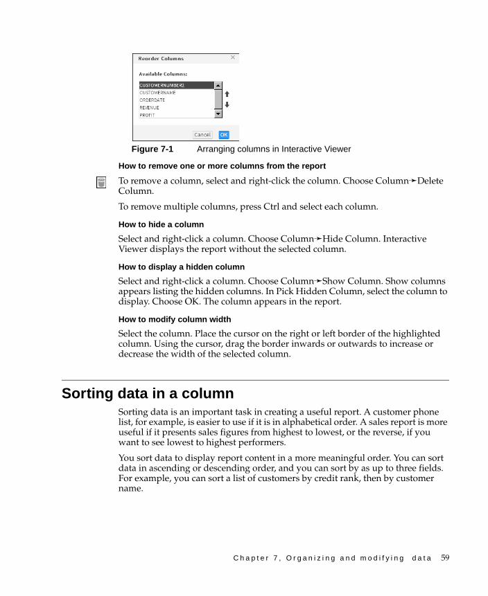
C h a p t e r 7 , O r g a n i z i n g a n d m o d i f y i n g d a t a 59
Figure 7-1 Arranging columns in Interactive Viewer
How to remove one or more columns from the report
To remove a column, select and right-click the column. Choose Column➛Delete Column.
To remove multiple columns, press Ctrl and select each column.
How to hide a column
Select and right-click a column. Choose Column➛Hide Column. Interactive Viewer displays the report without the selected column.
How to display a hidden column
Select and right-click a column. Choose Column➛Show Column. Show columns appears listing the hidden columns. In Pick Hidden Column, select the column to display. Choose OK. The column appears in the report.
How to modify column width
Select the column. Place the cursor on the right or left border of the highlighted column. Using the cursor, drag the border inwards or outwards to increase or decrease the width of the selected column.
Sorting data in a columnSorting data is an important task in creating a useful report. A customer phone list, for example, is easier to use if it is in alphabetical order. A sales report is more useful if it presents sales figures from highest to lowest, or the reverse, if you want to see lowest to highest performers.
You sort data to display report content in a more meaningful order. You can sort data in ascending or descending order, and you can sort by as up to three fields. For example, you can sort a list of customers by credit rank, then by customer name.
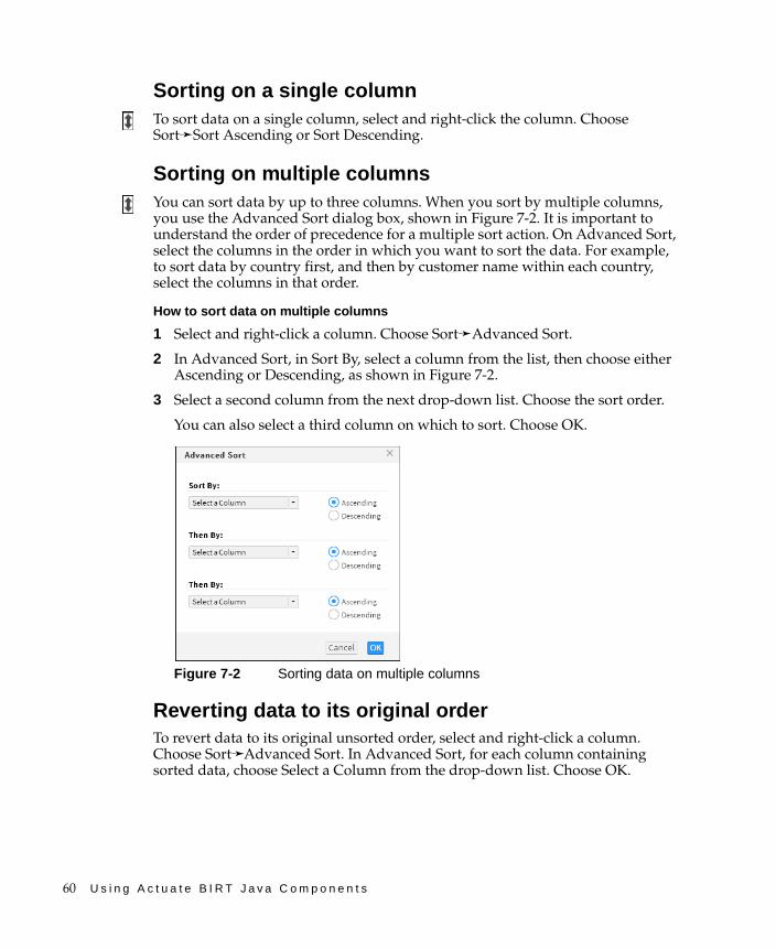
60 U s i n g A c t u a t e B I R T J a v a C o m p o n e n t s
Sorting on a single columnTo sort data on a single column, select and right-click the column. Choose Sort➛Sort Ascending or Sort Descending.
Sorting on multiple columnsYou can sort data by up to three columns. When you sort by multiple columns, you use the Advanced Sort dialog box, shown in Figure 7-2. It is important to understand the order of precedence for a multiple sort action. On Advanced Sort, select the columns in the order in which you want to sort the data. For example, to sort data by country first, and then by customer name within each country, select the columns in that order.
How to sort data on multiple columns
1 Select and right-click a column. Choose Sort➛Advanced Sort.
2 In Advanced Sort, in Sort By, select a column from the list, then choose either Ascending or Descending, as shown in Figure 7-2.
3 Select a second column from the next drop-down list. Choose the sort order.
You can also select a third column on which to sort. Choose OK.
Figure 7-2 Sorting data on multiple columns
Reverting data to its original orderTo revert data to its original unsorted order, select and right-click a column. Choose Sort➛Advanced Sort. In Advanced Sort, for each column containing sorted data, choose Select a Column from the drop-down list. Choose OK.
C h a p t e r 7 , O r g a n i z i n g a n d m o d i f y i n g d a t a 61
Organizing data in groups Sorting is typically only one of the tasks you perform when organizing data in a report. It is common for reports to present data that is organized into meaningful groups, especially reports that contain large amounts of data. Data groups contain related data rows. Organizing data in groups makes it easier to compare and analyze information.
A report that groups data provides a more effective way to view data. When you group data, you can:
■ Add subtotals, counts, averages, or other aggregate information at the beginning or end of each group.
■ Insert a page break before or after each group to start each data group on a new page.
■ Hide the details of each group to view a summary report.
In addition, Interactive Viewer performs the following actions when you group data:
■ Removes duplicate values for each group.
■ Sorts the values of each group. For example, a country group displays the countries in alphabetical order.
■ Generates a table of contents that displays the values of every group when you view the finished report in the viewers. The table of contents allows you to navigate to specific locations in the report. This feature is particularly useful when a report contains many pages.
How to group data
Select and right-click the column that contains the values to group. Choose Group➛Add Group.
If the column you selected contains string or numeric data, Interactive Viewer groups the data by each unique value in the column. If the column you selected contains date-and-time data, additional grouping options appear.
Grouping data on a date-and-time columnWhen you group data on a date-and-time column, you have an additional option to group the data by a specific time interval, which is the typical option. You can organize a shipping report, for example, showing shipment data by month or by quarter, rather than by individual date.
Figure 7-3 shows three reports that contain the same data.
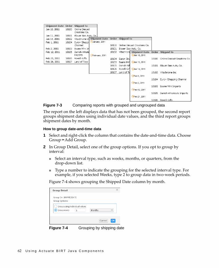
62 U s i n g A c t u a t e B I R T J a v a C o m p o n e n t s
Figure 7-3 Comparing reports with grouped and ungrouped data
The report on the left displays data that has not been grouped, the second report groups shipment dates using individual date values, and the third report groups shipment dates by month.
How to group date-and-time data
1 Select and right-click the column that contains the date-and-time data. Choose Group➛Add Group.
2 In Group Detail, select one of the group options. If you opt to group by interval:
■ Select an interval type, such as weeks, months, or quarters, from the drop-down list.
■ Type a number to indicate the grouping for the selected interval type. For example, if you selected Weeks, type 2 to group data in two-week periods.
Figure 7-4 shows grouping the Shipped Date column by month.
Figure 7-4 Grouping by shipping date
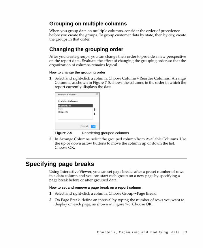
C h a p t e r 7 , O r g a n i z i n g a n d m o d i f y i n g d a t a 63
Grouping on multiple columnsWhen you group data on multiple columns, consider the order of precedence before you create the groups. To group customer data by state, then by city, create the groups in that order.
Changing the grouping orderAfter you create groups, you can change their order to provide a new perspective on the report data. Evaluate the effect of changing the grouping order, so that the organization of columns remains logical.
How to change the grouping order
1 Select and right-click a column. Choose Column➛Reorder Columns. Arrange Columns, as shown in Figure 7-5, shows the columns in the order in which the report currently displays the data.
Figure 7-5 Reordering grouped columns
2 In Arrange Columns, select the grouped column from Available Columns. Use the up or down arrow buttons to move the column up or down the list. Choose OK.
Specifying page breaksUsing Interactive Viewer, you can set page breaks after a preset number of rows in a data column and you can start each group on a new page by specifying a page break before or after grouped data.
How to set and remove a page break on a report column
1 Select and right-click a column. Choose Group➛Page Break.
2 On Page Break, define an interval by typing the number of rows you want to display on each page, as shown in Figure 7-6. Choose OK.

64 U s i n g A c t u a t e B I R T J a v a C o m p o n e n t s
Figure 7-6 Setting a page break on a data column
3 To delete an existing page break, type 0 in the Interval field. Choose OK.
How to set and remove a page break on a grouped column
1 Select and right-click a grouped column. Choose Group➛Page Break. Page Break appears, as shown in Figure 7-7.
Figure 7-7 Setting a page break before or after groups
2 You can set a page break for every group, or for every group except the first or last groups. Choose OK.
3 To delete an existing page break, select None in Before group or After group. Choose OK.
Inserting a computed columnTo display calculated data in a report, you create a computed column, such as the Total column in the report shown in Figure 7-8. In the example, you need to calculate the Total because the original report does not provide this data.
Figure 7-8 Report with computed column
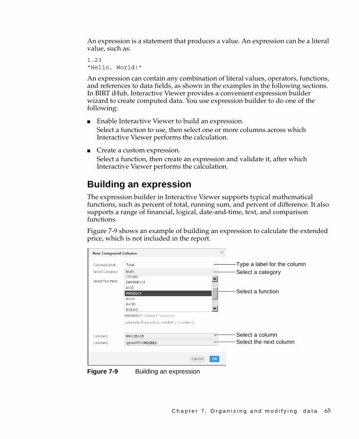
C h a p t e r 7 , O r g a n i z i n g a n d m o d i f y i n g d a t a 65
An expression is a statement that produces a value. An expression can be a literal value, such as:
1.23"Hello, World!"
An expression can contain any combination of literal values, operators, functions, and references to data fields, as shown in the examples in the following sections. In BIRT iHub, Interactive Viewer provides a convenient expression builder wizard to create computed data. You use expression builder to do one of the following:
■ Enable Interactive Viewer to build an expression.Select a function to use, then select one or more columns across which Interactive Viewer performs the calculation.
■ Create a custom expression.Select a function, then create an expression and validate it, after which Interactive Viewer performs the calculation.
Building an expressionThe expression builder in Interactive Viewer supports typical mathematical functions, such as percent of total, running sum, and percent of difference. It also supports a range of financial, logical, date-and-time, text, and comparison functions.
Figure 7-9 shows an example of building an expression to calculate the extended price, which is not included in the report.
Figure 7-9 Building an expression
Select a function
Select a column
Type a label for the column
Select the next column
Select a category
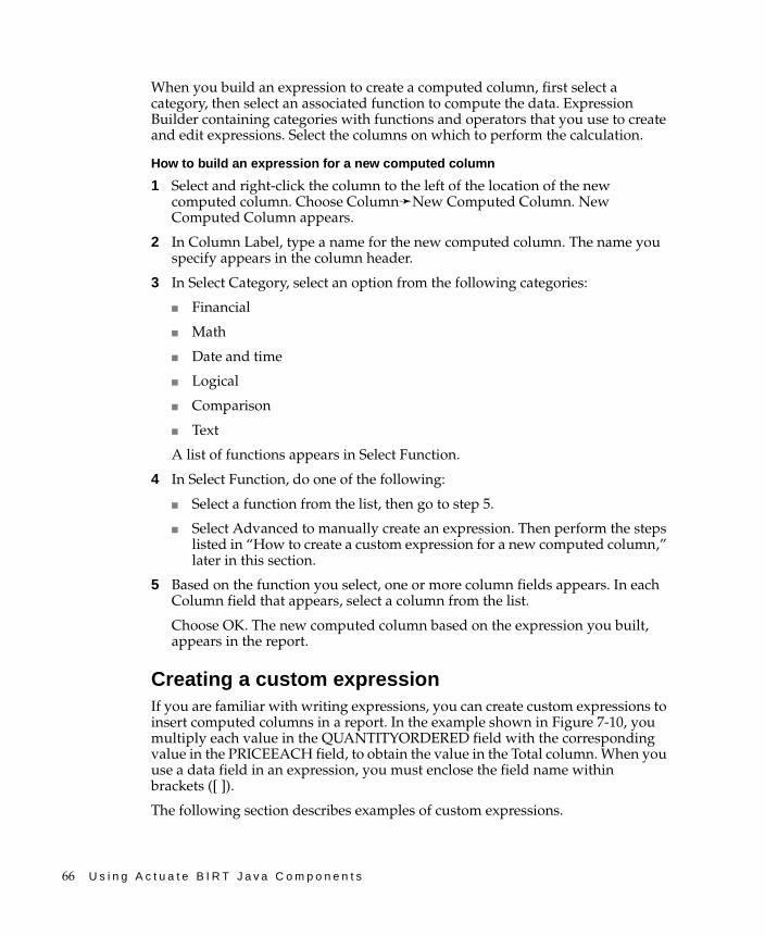
66 U s i n g A c t u a t e B I R T J a v a C o m p o n e n t s
When you build an expression to create a computed column, first select a category, then select an associated function to compute the data. Expression Builder containing categories with functions and operators that you use to create and edit expressions. Select the columns on which to perform the calculation.
How to build an expression for a new computed column
1 Select and right-click the column to the left of the location of the new computed column. Choose Column➛New Computed Column. New Computed Column appears.
2 In Column Label, type a name for the new computed column. The name you specify appears in the column header.
3 In Select Category, select an option from the following categories:
■ Financial
■ Math
■ Date and time
■ Logical
■ Comparison
■ Text
A list of functions appears in Select Function.
4 In Select Function, do one of the following:
■ Select a function from the list, then go to step 5.
■ Select Advanced to manually create an expression. Then perform the steps listed in “How to create a custom expression for a new computed column,” later in this section.
5 Based on the function you select, one or more column fields appears. In each Column field that appears, select a column from the list.
Choose OK. The new computed column based on the expression you built, appears in the report.
Creating a custom expressionIf you are familiar with writing expressions, you can create custom expressions to insert computed columns in a report. In the example shown in Figure 7-10, you multiply each value in the QUANTITYORDERED field with the corresponding value in the PRICEEACH field, to obtain the value in the Total column. When you use a data field in an expression, you must enclose the field name within brackets ([ ]).
The following section describes examples of custom expressions.
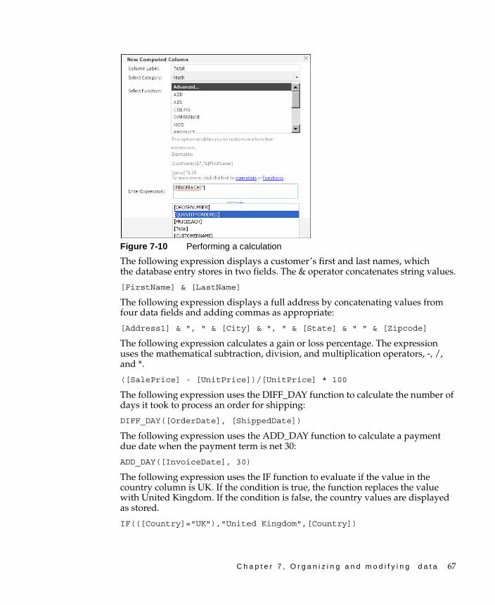
C h a p t e r 7 , O r g a n i z i n g a n d m o d i f y i n g d a t a 67
Figure 7-10 Performing a calculation
The following expression displays a customer’s first and last names, which the database entry stores in two fields. The & operator concatenates string values.
[FirstName] & [LastName]
The following expression displays a full address by concatenating values from four data fields and adding commas as appropriate:
[Address1] & ", " & [City] & ", " & [State] & " " & [Zipcode]
The following expression calculates a gain or loss percentage. The expression uses the mathematical subtraction, division, and multiplication operators, -, /, and *.
([SalePrice] - [UnitPrice])/[UnitPrice] * 100
The following expression uses the DIFF_DAY function to calculate the number of days it took to process an order for shipping:
DIFF_DAY([OrderDate], [ShippedDate])
The following expression uses the ADD_DAY function to calculate a payment due date when the payment term is net 30:
ADD_DAY([InvoiceDate], 30)
The following expression uses the IF function to evaluate if the value in the country column is UK. If the condition is true, the function replaces the value with United Kingdom. If the condition is false, the country values are displayed as stored.
IF(([Country]="UK"),"United Kingdom",[Country])
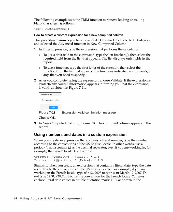
68 U s i n g A c t u a t e B I R T J a v a C o m p o n e n t s
The following example uses the TRIM function to remove leading or trailing blank characters, as follows:
TRIM([CustomerName])
How to create a custom expression for a new computed column
This procedure assumes you have provided a Column Label, selected a Category, and selected the Advanced function in New Computed Column.
1 In Enter Expression, type the expression that performs the calculation:
■ To use a data field in the expression, type the left bracket ([), then select the required field from the list that appears. The list displays only fields in the report.
■ To use a function, type the first letter of the function, then select the function from the list that appears. The functions indicate the arguments, if any, that you need to specify.
2 After you complete typing the expression, choose Validate. If the expression is syntactically correct, Information appears informing you that the expression is valid, as shown in Figure 7-11.
Figure 7-11 Expression valid confirmation message
Choose OK.
3 In New Computed Column, choose OK. The computed column appears in the report.
Using numbers and dates in a custom expressionWhen you create an expression that contains a literal number, type the number according to the conventions of the US English locale. In other words, use a period (.), not a comma (,) as the decimal separator, even if you are working in, for example, the French locale. For example:
Correct: ([Quantity] * [Price]) * 1.5Incorrect: ([Quantity] * [Price]) * 1,5
Similarly, when you create an expression that contains a literal date, type the date according to the conventions of the US English locale. For example, if you are working in the French locale, type 03/12/2007 to represent March 12, 2007. Do not type 12/03/2007, which is the convention for the French locale. You must enclose literal date values in double quotation marks (" "), as shown in the
C h a p t e r 7 , O r g a n i z i n g a n d m o d i f y i n g d a t a 69
following expression that calculates the number of days from the order date to Christmas:
DIFF_DAY([OrderDate], "12/25/08")
How to add days to an existing date value
To create a column that displays date values that are greater than the date values in another column, complete the following steps.
1 Select and right-click a column. Choose Column➛New Computed Column. New Computed Column appears.
2 In Column Label, type a name for the calculated column. For example, type Forecast Shipping Date.
3 In Enter Expression, type the letter A. A list appears, displaying functions that begin with A.
4 Choose ADD_DAY(date, daysToAdd).
5 For the first argument, type a left bracket ([) and select the date column from the list. For example, select Order Date.
6 For the second argument, type the number of days to add. In this case, type 7.
7 Validate the expression and choose OK. The calculated column appears in the report. For every value in the Order Date column, the calculated column displays a date seven days later than the order date.
How to subtract date values in a calculated column
The following section describes how to display the difference between two date values.
1 Select and right-click a column. Choose Column➛New Computed Column. New Computed Column appears.
2 In Column Label, type a name for the calculated column. For example, for a calculation that subtracts the actual shipping date from the date requested, type Shipping Delay.
3 In Enter Expression, type the letter d. A list appears, displaying functions that begin with d.
4 Choose DIFF_DAY(date1, date2).
5 For the first argument, type a left bracket ([) and select the first date column from the list. For example, select Date Requested.
6 For the second argument, type a left bracket ([) and select the second date column from the list. For example, select Actual Shipping Date.
7 Validate the expression and choose OK. The calculated column appears in the report, displaying the difference between the two dates.
70 U s i n g A c t u a t e B I R T J a v a C o m p o n e n t s
Using reserved characters in a custom expressionSome characters are reserved for internal use and have a special meaning. For example, Interactive Viewer uses brackets to denote a data field. The following characters are reserved in Interactive Viewer:
[]?' (single quotation mark)
If the name of a data field contains a reserved character, Interactive Viewer encloses the reserved character in single quotes (') when you select the data field for use in an expression, for example '['. If the name of a data field is OBSOLETE?, Interactive Viewer changes it to [OBSOLETE'?'] in the expression. If you type [OBSOLETE?] in the expression, the dialog box displays an error message.
To minimize syntax errors, select the field from the list in the New Computed Column dialog box and allow the software to construct the expression, instead of typing it yourself. The following examples shows the appearance of data fields containing reserved characters in the New Computed Column dialog box. The examples show both versions of the names, the changed name and the original name with reserved characters, as follows:
[ORDER'''S STATUS] - ORDER'S STATUS[PRODUCTCODE'['4-digit']'] - PRODUCTCODE[4-digit][OBSOLETE'?'] - OBSOLETE?
Aggregating dataOne of the useful features in a report is the ability to display summary, or aggregate, data. Aggregating data involves performing a calculation on a set of values. For a simple listing report that does not organize data in groups, you can perform aggregate calculations on values in a selected column, across all the data rows in a table. For example, consider a report that has a column calculating price*quantity. You can use the sum of the calculations in this column to obtain the total price of all items. You can create up to three aggregations for each report column.
When you aggregate data, you choose whether the aggregation appears in the table header or footer. If the column is grouped, you can display the aggregate value in the group header or footer. The report in Figure 7-12 displays aggregate data for the Total and the Profit columns at the end, or footer, of the table.
In a report that organizes data in groups, you can perform aggregations for each group of data rows, and for all the data rows in the table. In the example report shown in Figure 7-13, the aggregate data appears at the footer of each group.
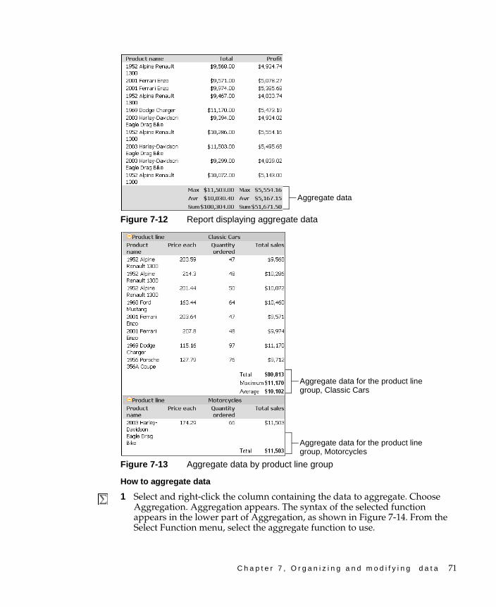
C h a p t e r 7 , O r g a n i z i n g a n d m o d i f y i n g d a t a 71
Figure 7-12 Report displaying aggregate data
Figure 7-13 Aggregate data by product line group
How to aggregate data
1 Select and right-click the column containing the data to aggregate. Choose Aggregation. Aggregation appears. The syntax of the selected function appears in the lower part of Aggregation, as shown in Figure 7-14. From the Select Function menu, select the aggregate function to use.
Aggregate data
Aggregate data for the product line group, Classic Cars
Aggregate data for the product line group, Motorcycles
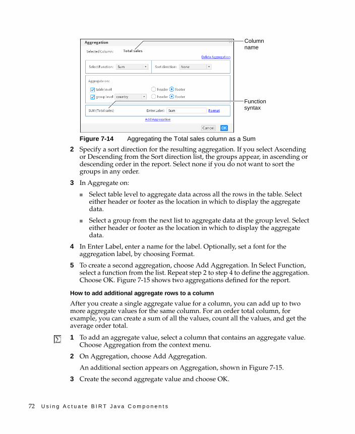
72 U s i n g A c t u a t e B I R T J a v a C o m p o n e n t s
Figure 7-14 Aggregating the Total sales column as a Sum
2 Specify a sort direction for the resulting aggregation. If you select Ascending or Descending from the Sort direction list, the groups appear, in ascending or descending order in the report. Select none if you do not want to sort the groups in any order.
3 In Aggregate on:
■ Select table level to aggregate data across all the rows in the table. Select either header or footer as the location in which to display the aggregate data.
■ Select a group from the next list to aggregate data at the group level. Select either header or footer as the location in which to display the aggregate data.
4 In Enter Label, enter a name for the label. Optionally, set a font for the aggregation label, by choosing Format.
5 To create a second aggregation, choose Add Aggregation. In Select Function, select a function from the list. Repeat step 2 to step 4 to define the aggregation. Choose OK. Figure 7-15 shows two aggregations defined for the report.
How to add additional aggregate rows to a column
After you create a single aggregate value for a column, you can add up to two more aggregate values for the same column. For an order total column, for example, you can create a sum of all the values, count all the values, and get the average order total.
1 To add an aggregate value, select a column that contains an aggregate value. Choose Aggregation from the context menu.
2 On Aggregation, choose Add Aggregation.
An additional section appears on Aggregation, shown in Figure 7-15.
3 Create the second aggregate value and choose OK.
Column name
Function syntax
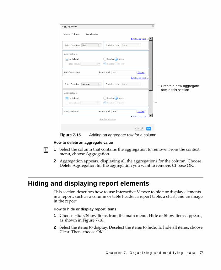
C h a p t e r 7 , O r g a n i z i n g a n d m o d i f y i n g d a t a 73
Figure 7-15 Adding an aggregate row for a column
How to delete an aggregate value
1 Select the column that contains the aggregation to remove. From the context menu, choose Aggregation.
2 Aggregation appears, displaying all the aggregations for the column. Choose Delete Aggregation for the aggregation you want to remove. Choose OK.
Hiding and displaying report elementsThis section describes how to use Interactive Viewer to hide or display elements in a report, such as a column or table header, a report table, a chart, and an image in the report.
How to hide or display report items
1 Choose Hide/Show Items from the main menu. Hide or Show Items appears, as shown in Figure 7-16.
2 Select the items to display. Deselect the items to hide. To hide all items, choose Clear. Then, choose OK.
Create a new aggregate row in this section

74 U s i n g A c t u a t e B I R T J a v a C o m p o n e n t s
Figure 7-16 Hiding or displaying report items
Hiding group detailsWhen you work with a report that organizes data in groups, you can change the report to a summary report by hiding the group details. Hiding details, particularly for a report that runs into hundreds of pages, helps you display key information at a glance.
In a report containing multiple groups, it is sometimes useful to hide the details for a specific group if you do not want to display all the information at the same time. Figure 7-17 shows two reports that contain the same data. The report on the left shows all details. The report on the right hides the details within each product line group.
Figure 7-17 Comparing reports showing and hiding product details
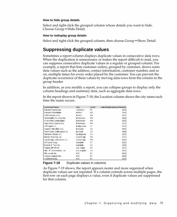
C h a p t e r 7 , O r g a n i z i n g a n d m o d i f y i n g d a t a 75
How to hide group details
Select and right-click the grouped column whose details you want to hide. Choose Group➛Hide Detail.
How to redisplay group details
Select and right-click the grouped column, then choose Group➛Show Detail.
Suppressing duplicate valuesSometimes a report column displays duplicate values in consecutive data rows. When the duplication is unnecessary or makes the report difficult to read, you can suppress consecutive duplicate values in a regular or grouped column. For example, a report that lists customer orders, grouped by customer, shows some data values such as the address, contact information, customer number, and so on, multiple times for every order placed by the customer. You can prevent the duplicate occurrence of these values by moving data rows from the column to the group header.
In addition, as you modify a report, you can collapse groups to display only the column headings and summary data, such as aggregate data rows.
In the report shown in Figure 7-18, the Location column shows the city name each time the name occurs.
Figure 7-18 Duplicate values in columns
As Figure 7-19 shows, the report appears neater and more organized when duplicate values are not repeated. If a column extends across multiple pages, the first row on each page displays a value, even if duplicate values are suppressed for that column.
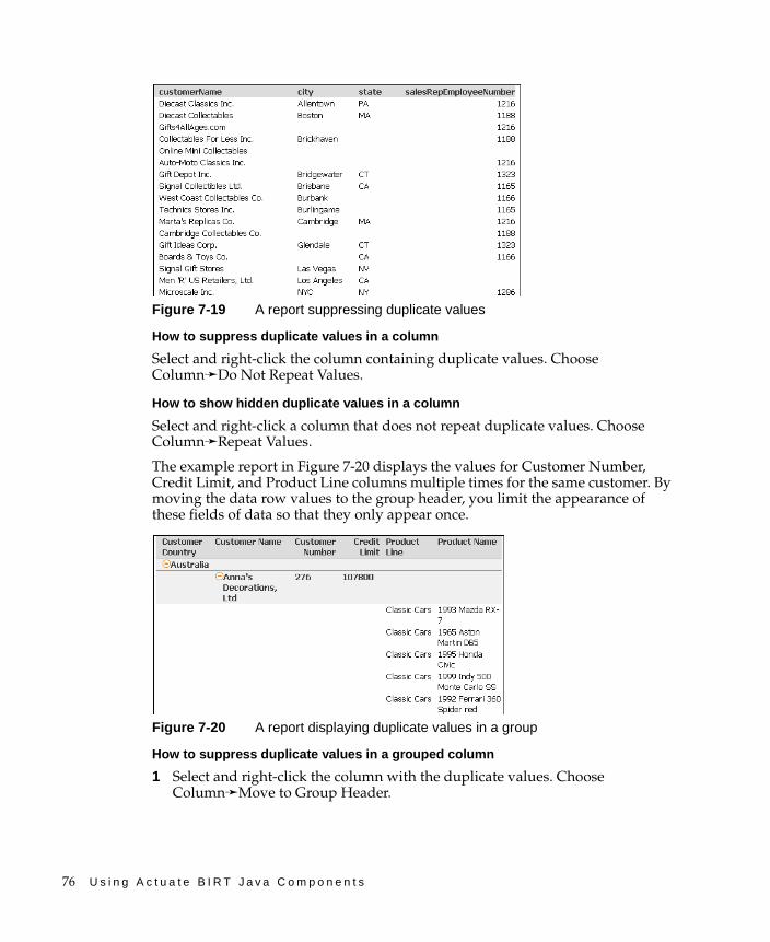
76 U s i n g A c t u a t e B I R T J a v a C o m p o n e n t s
Figure 7-19 A report suppressing duplicate values
How to suppress duplicate values in a column
Select and right-click the column containing duplicate values. Choose Column➛Do Not Repeat Values.
How to show hidden duplicate values in a column
Select and right-click a column that does not repeat duplicate values. Choose Column➛Repeat Values.
The example report in Figure 7-20 displays the values for Customer Number, Credit Limit, and Product Line columns multiple times for the same customer. By moving the data row values to the group header, you limit the appearance of these fields of data so that they only appear once.
Figure 7-20 A report displaying duplicate values in a group
How to suppress duplicate values in a grouped column
1 Select and right-click the column with the duplicate values. Choose Column➛Move to Group Header.

C h a p t e r 7 , O r g a n i z i n g a n d m o d i f y i n g d a t a 77
2 On Move to Group Header, as shown in Figure 7-21, perform the following tasks:
■ Select the group to which you want to move the data values, if the report contains more than one group.
■ Select the header row to which Interactive Viewer can move the data values.
Figure 7-21 Selecting a group header
Repeat this step for each report column for which you want to move data rows to the group header. Choose OK. The value from the first data row in each group appears in each group header. The Customer Number, Credit Limit, and Product Line columns display a single data row for each Customer Name group header, as shown in Figure 7-22.
Figure 7-22 Displaying a report showing suppressed duplicate values
Filtering dataFiltering enables you to present the information that answers specific business questions, such as which sales representatives generated the top ten sales accounts, which products generated the highest profit in the last quarter, which customers have not made a purchase in the past 90 days, and so on.
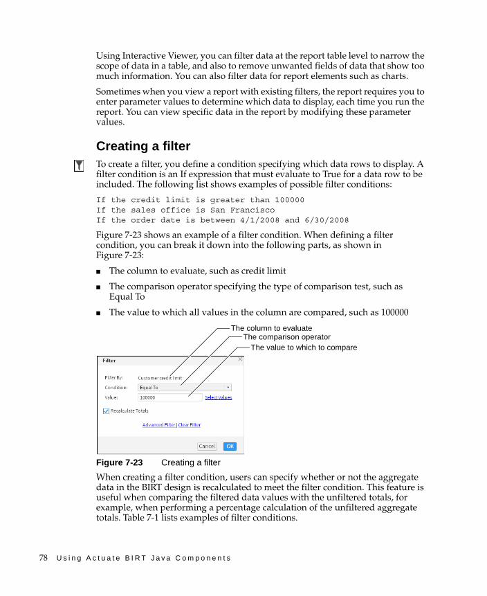
78 U s i n g A c t u a t e B I R T J a v a C o m p o n e n t s
Using Interactive Viewer, you can filter data at the report table level to narrow the scope of data in a table, and also to remove unwanted fields of data that show too much information. You can also filter data for report elements such as charts.
Sometimes when you view a report with existing filters, the report requires you to enter parameter values to determine which data to display, each time you run the report. You can view specific data in the report by modifying these parameter values.
Creating a filterTo create a filter, you define a condition specifying which data rows to display. A filter condition is an If expression that must evaluate to True for a data row to be included. The following list shows examples of possible filter conditions:
If the credit limit is greater than 100000If the sales office is San FranciscoIf the order date is between 4/1/2008 and 6/30/2008
Figure 7-23 shows an example of a filter condition. When defining a filter condition, you can break it down into the following parts, as shown in Figure 7-23:
■ The column to evaluate, such as credit limit
■ The comparison operator specifying the type of comparison test, such as Equal To
■ The value to which all values in the column are compared, such as 100000
Figure 7-23 Creating a filter
When creating a filter condition, users can specify whether or not the aggregate data in the BIRT design is recalculated to meet the filter condition. This feature is useful when comparing the filtered data values with the unfiltered totals, for example, when performing a percentage calculation of the unfiltered aggregate totals. Table 7-1 lists examples of filter conditions.
The value to which to compare The comparison operator
The column to evaluate
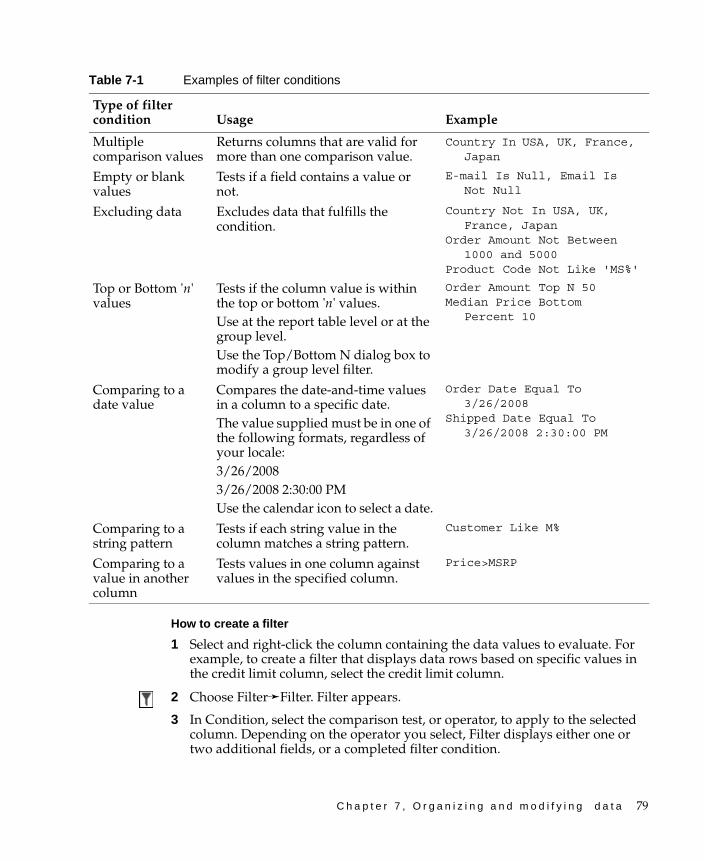
C h a p t e r 7 , O r g a n i z i n g a n d m o d i f y i n g d a t a 79
How to create a filter
1 Select and right-click the column containing the data values to evaluate. For example, to create a filter that displays data rows based on specific values in the credit limit column, select the credit limit column.
2 Choose Filter➛Filter. Filter appears.
3 In Condition, select the comparison test, or operator, to apply to the selected column. Depending on the operator you select, Filter displays either one or two additional fields, or a completed filter condition.
Table 7-1 Examples of filter conditions
Type of filter condition Usage Example
Multiple comparison values
Returns columns that are valid for more than one comparison value.
Country In USA, UK, France, Japan
Empty or blank values
Tests if a field contains a value or not.
E-mail Is Null, Email Is Not Null
Excluding data Excludes data that fulfills the condition.
Country Not In USA, UK, France, Japan
Order Amount Not Between 1000 and 5000
Product Code Not Like 'MS%'
Top or Bottom 'n' values
Tests if the column value is within the top or bottom 'n' values. Use at the report table level or at the group level. Use the Top/Bottom N dialog box to modify a group level filter.
Order Amount Top N 50Median Price Bottom
Percent 10
Comparing to a date value
Compares the date-and-time values in a column to a specific date.The value supplied must be in one of the following formats, regardless of your locale:3/26/20083/26/2008 2:30:00 PMUse the calendar icon to select a date.
Order Date Equal To 3/26/2008
Shipped Date Equal To 3/26/2008 2:30:00 PM
Comparing to a string pattern
Tests if each string value in the column matches a string pattern.
Customer Like M%
Comparing to a value in another column
Tests values in one column against values in the specified column.
Price>MSRP

80 U s i n g A c t u a t e B I R T J a v a C o m p o n e n t s
4 If you select an operator that requires a comparison value, you can specify the value in one of the following ways:
■ Type the value.
■ Choose Select Values to select from a list of existing data values. Figure 7-24 shows how you can select a credit limit value of 11000 from the list of possible credit limit values. Use the Previous and Next buttons to navigate the list of values that appears.
■ Select or deselect Recalculate Totals based on whether you want the aggregate data in the report to be modified or not. Choose OK.
Choose OK to apply the filter. If the report or report element such as chart, contains no data that matches the filter condition, Interactive Viewer does not display any data. Make sure you test the filter by applying it and viewing the resulting report.
Figure 7-24 Selecting a value for the filter condition
When you create a filter condition on a column containing Float or Double data type, the In or Equal to operators do not work as expected in Java-based applications. To make sure you obtain the results you expect, do one of the following:
■ When using the In operator in a filter condition specified on a computed column, make sure you round the values in the column to a specified number of digits. For example, the following expression rounds the value obtained by three decimal places:
ROUND([dbo_ITEMS:PRICEQUOTE]*[dbo_ITEMS:QUANTITY]*0.001, 3)
■ Use the Between operator in filter conditions in place of the Equal to operator.
Selecting multiple values for a filter conditionSometimes you need to view a wider range of data, such as sales details for several sales offices, not only for a single office, as shown in Figure 7-25.
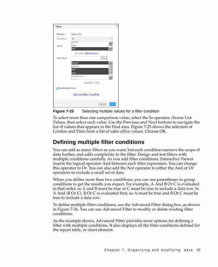
C h a p t e r 7 , O r g a n i z i n g a n d m o d i f y i n g d a t a 81
Figure 7-25 Selecting multiple values for a filter condition
To select more than one comparison value, select the In operator, choose List Values, then select each value. Use the Previous and Next buttons to navigate the list of values that appears in the Find area. Figure 7-25 shows the selection of London and Paris from a list of sales office values. Choose OK.
Defining multiple filter conditionsYou can add as many filters as you want, but each condition narrows the scope of data further, and adds complexity to the filter. Design and test filters with multiple conditions carefully. As you add filter conditions, Interactive Viewer inserts the logical operator And between each filter expression. You can change this operator to Or. You can also add the Not operator to either the And or Or operators to exclude a small set of data.
When you define more than two conditions, you can use parentheses to group conditions to get the results you expect. For example, A And B Or C is evaluated in that order, so A and B must be true or C must be true to include a data row. In A And (B Or C), B Or C is evaluated first, so A must be true and B Or C must be true to include a data row.
To define multiple filter conditions, use the Advanced Filter dialog box, as shown in Figure 7-26. You can use Advanced Filter to modify or delete existing filter conditions.
As the example shows, Advanced Filter provides more options for defining a filter with multiple conditions. It also displays all the filter conditions defined for the report table, or chart element.
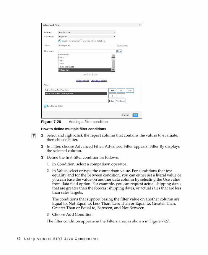
82 U s i n g A c t u a t e B I R T J a v a C o m p o n e n t s
Figure 7-26 Adding a filter condition
How to define multiple filter conditions
1 Select and right-click the report column that contains the values to evaluate, then choose Filter.
2 In Filter, choose Advanced Filter. Advanced Filter appears. Filter By displays the selected column.
3 Define the first filter condition as follows:
1 In Condition, select a comparison operator.
2 In Value, select or type the comparison value. For conditions that test equality and for the Between condition, you can either set a literal value or you can base the value on another data column by selecting the Use value from data field option. For example, you can request actual shipping dates that are greater than the forecast shipping dates, or actual sales that are less than sales targets.
The conditions that support basing the filter value on another column are Equal to, Not Equal to, Less Than, Less Than or Equal to, Greater Than, Greater Than or Equal to, Between, and Not Between.
3 Choose Add Condition.
The filter condition appears in the Filters area, as shown in Figure 7-27.
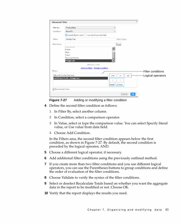
C h a p t e r 7 , O r g a n i z i n g a n d m o d i f y i n g d a t a 83
Figure 7-27 Adding or modifying a filter condition
4 Define the second filter condition as follows:
1 In Filter By, select another column.
2 In Condition, select a comparison operator.
3 In Value, select or type the comparison value. You can select Specify literal value, or Use value from data field.
4 Choose Add Condition.
In the Filters area, the second filter condition appears below the first condition, as shown in Figure 7-27. By default, the second condition is preceded by the logical operator, AND.
5 Choose a different logical operator, if necessary.
6 Add additional filter conditions using the previously outlined method.
7 If you create more than two filter conditions and you use different logical operators, you can use the Parentheses buttons to group conditions and define the order of evaluation of the filter conditions.
8 Choose Validate to verify the syntax of the filter conditions.
9 Select or deselect Recalculate Totals based on whether you want the aggregate data in the report to be modified or not. Choose OK.
10 Verify that the report displays the results you need.
Logical operatorsFilter conditions
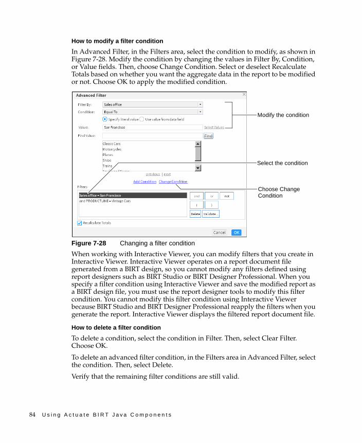
84 U s i n g A c t u a t e B I R T J a v a C o m p o n e n t s
How to modify a filter condition
In Advanced Filter, in the Filters area, select the condition to modify, as shown in Figure 7-28. Modify the condition by changing the values in Filter By, Condition, or Value fields. Then, choose Change Condition. Select or deselect Recalculate Totals based on whether you want the aggregate data in the report to be modified or not. Choose OK to apply the modified condition.
Figure 7-28 Changing a filter condition
When working with Interactive Viewer, you can modify filters that you create in Interactive Viewer. Interactive Viewer operates on a report document file generated from a BIRT design, so you cannot modify any filters defined using report designers such as BIRT Studio or BIRT Designer Professional. When you specify a filter condition using Interactive Viewer and save the modified report as a BIRT design file, you must use the report designer tools to modify this filter condition. You cannot modify this filter condition using Interactive Viewer because BIRT Studio and BIRT Designer Professional reapply the filters when you generate the report. Interactive Viewer displays the filtered report document file.
How to delete a filter condition
To delete a condition, select the condition in Filter. Then, select Clear Filter. Choose OK.
To delete an advanced filter condition, in the Filters area in Advanced Filter, select the condition. Then, select Delete.
Verify that the remaining filter conditions are still valid.
Select the condition
Modify the condition
Choose Change Condition
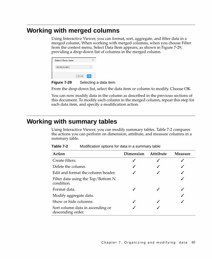
C h a p t e r 7 , O r g a n i z i n g a n d m o d i f y i n g d a t a 85
Working with merged columnsUsing Interactive Viewer, you can format, sort, aggregate, and filter data in a merged column, When working with merged columns, when you choose Filter from the context menu, Select Data Item appears, as shown in Figure 7-29, providing a drop-down list of columns in the merged column.
Figure 7-29 Selecting a data item
From the drop-down list, select the data item or column to modify. Choose OK.
You can now modify data in the column as described in the previous sections of this document. To modify each column in the merged column, repeat this step for each data item, and specify a modification action.
Working with summary tablesUsing Interactive Viewer, you can modify summary tables. Table 7-2 compares the actions you can perform on dimension, attribute, and measure columns in a summary table.
Table 7-2 Modification options for data in a summary table
Action Dimension Attribute Measure
Create filters. ✓ ✓ ✓
Delete the column. ✓ ✓ ✓
Edit and format the column header. ✓ ✓ ✓
Filter data using the Top/Bottom N condition.
✓
Format data. ✓ ✓ ✓
Modify aggregate data. ✓
Show or hide columns. ✓ ✓ ✓
Sort column data in ascending or descending order.
✓ ✓

86 U s i n g A c t u a t e B I R T J a v a C o m p o n e n t s
C h a p t e r 8 , M o d i f y i n g c h a r t s 87
C h a p t e r
8Chapter 8Modifying charts
This chapter contains the following topics:
■ About charts
■ Types of charts
■ Modifying charts
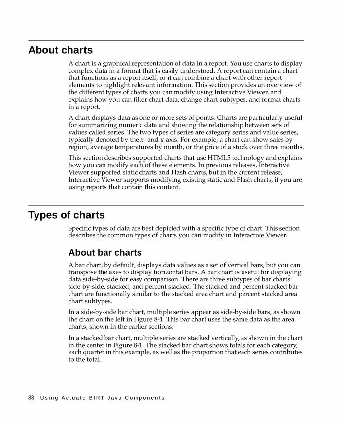
88 U s i n g A c t u a t e B I R T J a v a C o m p o n e n t s
About chartsA chart is a graphical representation of data in a report. You use charts to display complex data in a format that is easily understood. A report can contain a chart that functions as a report itself, or it can combine a chart with other report elements to highlight relevant information. This section provides an overview of the different types of charts you can modify using Interactive Viewer, and explains how you can filter chart data, change chart subtypes, and format charts in a report.
A chart displays data as one or more sets of points. Charts are particularly useful for summarizing numeric data and showing the relationship between sets of values called series. The two types of series are category series and value series, typically denoted by the x- and y-axis. For example, a chart can show sales by region, average temperatures by month, or the price of a stock over three months.
This section describes supported charts that use HTML5 technology and explains how you can modify each of these elements. In previous releases, Interactive Viewer supported static charts and Flash charts, but in the current release, Interactive Viewer supports modifying existing static and Flash charts, if you are using reports that contain this content.
Types of chartsSpecific types of data are best depicted with a specific type of chart. This section describes the common types of charts you can modify in Interactive Viewer.
About bar chartsA bar chart, by default, displays data values as a set of vertical bars, but you can transpose the axes to display horizontal bars. A bar chart is useful for displaying data side-by-side for easy comparison. There are three subtypes of bar charts: side-by-side, stacked, and percent stacked. The stacked and percent stacked bar chart are functionally similar to the stacked area chart and percent stacked area chart subtypes.
In a side-by-side bar chart, multiple series appear as side-by-side bars, as shown the chart on the left in Figure 8-1. This bar chart uses the same data as the area charts, shown in the earlier sections.
In a stacked bar chart, multiple series are stacked vertically, as shown in the chart in the center in Figure 8-1. The stacked bar chart shows totals for each category, each quarter in this example, as well as the proportion that each series contributes to the total.
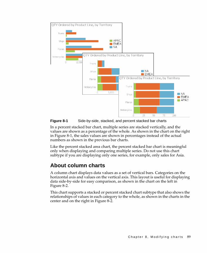
C h a p t e r 8 , M o d i f y i n g c h a r t s 89
Figure 8-1 Side-by-side, stacked, and percent stacked bar charts
In a percent stacked bar chart, multiple series are stacked vertically, and the values are shown as a percentage of the whole. As shown in the chart on the right in Figure 8-1, the sales values are shown in percentages instead of the actual numbers as shown in the previous bar charts.
Like the percent stacked area chart, the percent stacked bar chart is meaningful only when displaying and comparing multiple series. Do not use this chart subtype if you are displaying only one series, for example, only sales for Asia.
About column chartsA column chart displays data values as a set of vertical bars. Categories on the horizontal axis and values on the vertical axis. This layout is useful for displaying data side-by-side for easy comparison, as shown in the chart on the left in Figure 8-2.
This chart supports a stacked or percent stacked chart subtype that also shows the relationships of values in each category to the whole, as shown in the charts in the center and on the right in Figure 8-2.
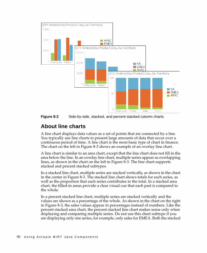
90 U s i n g A c t u a t e B I R T J a v a C o m p o n e n t s
Figure 8-2 Side-by-side, stacked, and percent stacked column charts
About line chartsA line chart displays data values as a set of points that are connected by a line. You typically use line charts to present large amounts of data that occur over a continuous period of time. A line chart is the most basic type of chart in finance. The chart on the left in Figure 8-3 shows an example of an overlay line chart.
A line chart is similar to an area chart, except that the line chart does not fill in the area below the line. In an overlay line chart, multiple series appear as overlapping lines, as shown in the chart on the left in Figure 8-3. The line chart supports stacked and percent stacked subtypes.
In a stacked line chart, multiple series are stacked vertically, as shown in the chart in the center in Figure 8-3. The stacked line chart shows totals for each series, as well as the proportion that each series contributes to the total. In a stacked area chart, the filled-in areas provide a clear visual cue that each part is compared to the whole.
In a percent stacked line chart, multiple series are stacked vertically and the values are shown as a percentage of the whole. As shown in the chart on the right in Figure 8-3, the sales values appear in percentages instead of numbers. Like the percent stacked area chart, the percent stacked line chart makes sense only when displaying and comparing multiple series. Do not use this chart subtype if you are displaying only one series, for example, only sales for EMEA. Both the stacked

C h a p t e r 8 , M o d i f y i n g c h a r t s 91
line chart and the percent stacked line chart are not as effective as their area chart counterparts.
Figure 8-3 Overlay, stacked, and percent stacked line charts
In addition, as the example shows, a user can easily misinterpret the data in a stacked line chart. There is no obvious indication that the top line shows the total sales amount for each quarter, and the middle line shows the difference in the sales amount between EMEA and APAC.
About meter chartsA meter chart displays a value as a needle pointer on a semicircle, called a dial. As Figure 8-4 shows, a meter chart resembles a speedometer, with tick marks and numbers showing a range of values. A meter chart supports standard and superimposed subtypes.
The standard meter chart typically creates a dashboard effect, which is visually compelling. A standard meter chart displays multiple values in multiple dials, where each dial displays a single value, as shown in the chart on the left in Figure 8-4. The chart in this example displays quantities ordered by product line. A superimposed meter chart displays multiple values in a single dial, as shown in the chart on the right in Figure 8-5. Use the superimposed meter chart type when there are few values to display and when each value is distinct. Duplicate values result in overlapping needles. The data used in the example is better suited for display in a standard meter chart. Because the same data displays too many values in the superimposed meter chart on the left in Figure 8-5, it is not easy to
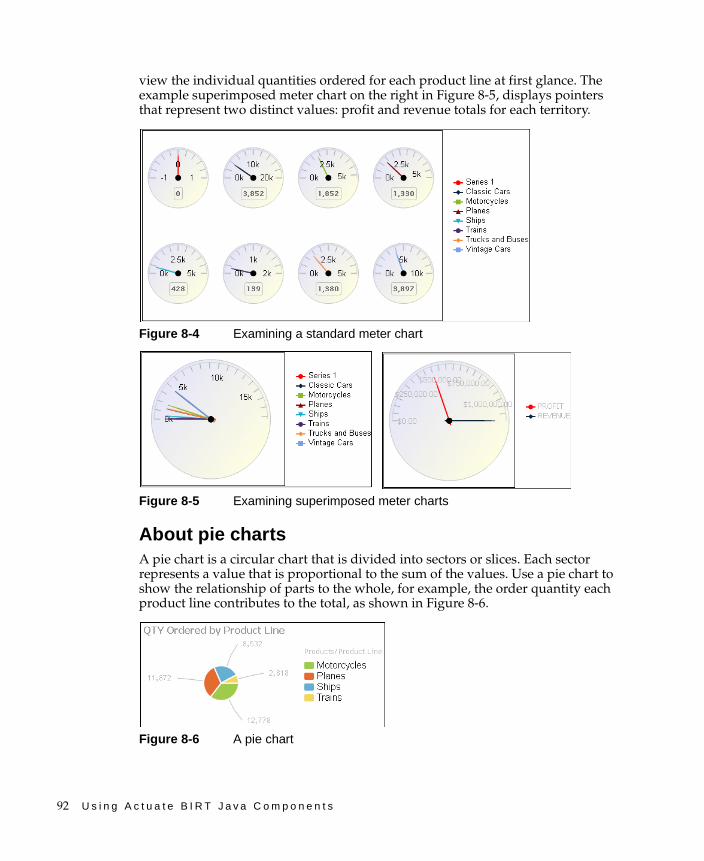
92 U s i n g A c t u a t e B I R T J a v a C o m p o n e n t s
view the individual quantities ordered for each product line at first glance. The example superimposed meter chart on the right in Figure 8-5, displays pointers that represent two distinct values: profit and revenue totals for each territory.
Figure 8-4 Examining a standard meter chart
Figure 8-5 Examining superimposed meter charts
About pie chartsA pie chart is a circular chart that is divided into sectors or slices. Each sector represents a value that is proportional to the sum of the values. Use a pie chart to show the relationship of parts to the whole, for example, the order quantity each product line contributes to the total, as shown in Figure 8-6.
Figure 8-6 A pie chart
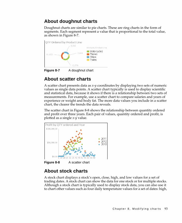
C h a p t e r 8 , M o d i f y i n g c h a r t s 93
About doughnut chartsDoughnut charts are similar to pie charts. These are ring charts in the form of segments. Each segment represent a value that is proportional to the total value, as shown in Figure 8-7.
Figure 8-7 A doughnut chart
About scatter chartsA scatter chart presents data as x-y coordinates by displaying two sets of numeric values as single data points. A scatter chart typically is used to display scientific and statistical data, because it shows if there is a relationship between two sets of measurements. For example, use a scatter chart to compare salaries and years of experience or weight and body fat. The more data values you include in a scatter chart, the clearer the trends the data reveals.
The scatter chart in Figure 8-8 shows the relationship between quantity ordered and profit over three years. Each pair of values, quantity ordered and profit, is plotted as a single x-y value.
Figure 8-8 A scatter chart
About stock chartsA stock chart displays a stock’s open, close, high, and low values for a set of trading dates. A stock chart can show the data for one stock or for multiple stocks. Although a stock chart is typically used to display stock data, you can also use it to chart other values such as four daily temperature values for a set of dates: high,
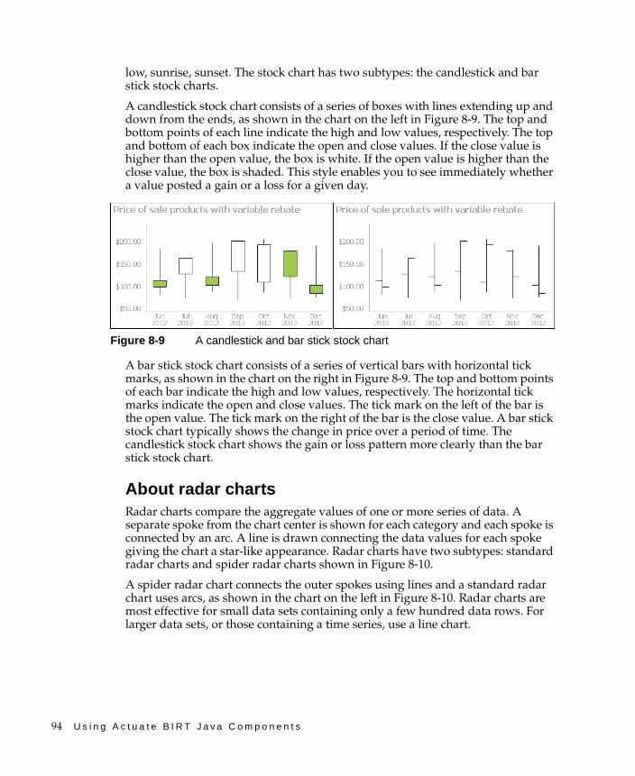
94 U s i n g A c t u a t e B I R T J a v a C o m p o n e n t s
low, sunrise, sunset. The stock chart has two subtypes: the candlestick and bar stick stock charts.
A candlestick stock chart consists of a series of boxes with lines extending up and down from the ends, as shown in the chart on the left in Figure 8-9. The top and bottom points of each line indicate the high and low values, respectively. The top and bottom of each box indicate the open and close values. If the close value is higher than the open value, the box is white. If the open value is higher than the close value, the box is shaded. This style enables you to see immediately whether a value posted a gain or a loss for a given day.
A bar stick stock chart consists of a series of vertical bars with horizontal tick marks, as shown in the chart on the right in Figure 8-9. The top and bottom points of each bar indicate the high and low values, respectively. The horizontal tick marks indicate the open and close values. The tick mark on the left of the bar is the open value. The tick mark on the right of the bar is the close value. A bar stick stock chart typically shows the change in price over a period of time. The candlestick stock chart shows the gain or loss pattern more clearly than the bar stick stock chart.
About radar chartsRadar charts compare the aggregate values of one or more series of data. A separate spoke from the chart center is shown for each category and each spoke is connected by an arc. A line is drawn connecting the data values for each spoke giving the chart a star-like appearance. Radar charts have two subtypes: standard radar charts and spider radar charts shown in Figure 8-10.
A spider radar chart connects the outer spokes using lines and a standard radar chart uses arcs, as shown in the chart on the left in Figure 8-10. Radar charts are most effective for small data sets containing only a few hundred data rows. For larger data sets, or those containing a time series, use a line chart.
Figure 8-9 A candlestick and bar stick stock chart
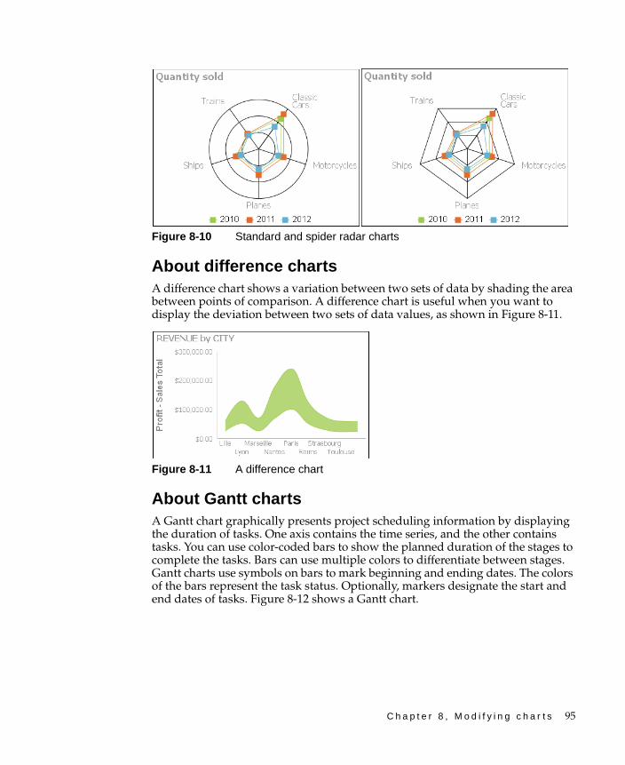
C h a p t e r 8 , M o d i f y i n g c h a r t s 95
Figure 8-10 Standard and spider radar charts
About difference chartsA difference chart shows a variation between two sets of data by shading the area between points of comparison. A difference chart is useful when you want to display the deviation between two sets of data values, as shown in Figure 8-11.
Figure 8-11 A difference chart
About Gantt chartsA Gantt chart graphically presents project scheduling information by displaying the duration of tasks. One axis contains the time series, and the other contains tasks. You can use color-coded bars to show the planned duration of the stages to complete the tasks. Bars can use multiple colors to differentiate between stages. Gantt charts use symbols on bars to mark beginning and ending dates. The colors of the bars represent the task status. Optionally, markers designate the start and end dates of tasks. Figure 8-12 shows a Gantt chart.
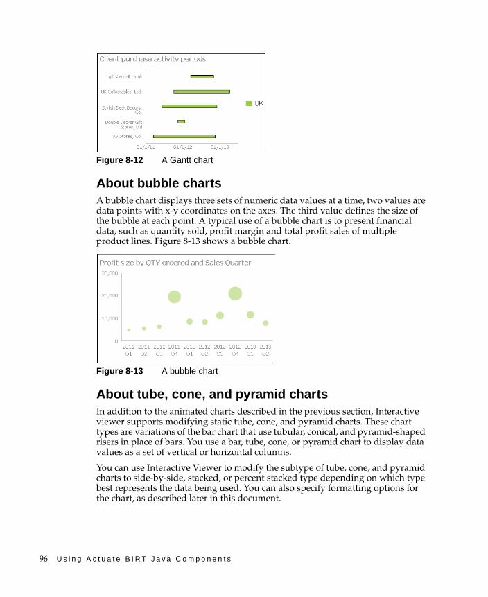
96 U s i n g A c t u a t e B I R T J a v a C o m p o n e n t s
Figure 8-12 A Gantt chart
About bubble chartsA bubble chart displays three sets of numeric data values at a time, two values are data points with x-y coordinates on the axes. The third value defines the size of the bubble at each point. A typical use of a bubble chart is to present financial data, such as quantity sold, profit margin and total profit sales of multiple product lines. Figure 8-13 shows a bubble chart.
Figure 8-13 A bubble chart
About tube, cone, and pyramid chartsIn addition to the animated charts described in the previous section, Interactive viewer supports modifying static tube, cone, and pyramid charts. These chart types are variations of the bar chart that use tubular, conical, and pyramid-shaped risers in place of bars. You use a bar, tube, cone, or pyramid chart to display data values as a set of vertical or horizontal columns.
You can use Interactive Viewer to modify the subtype of tube, cone, and pyramid charts to side-by-side, stacked, or percent stacked type depending on which type best represents the data being used. You can also specify formatting options for the chart, as described later in this document.
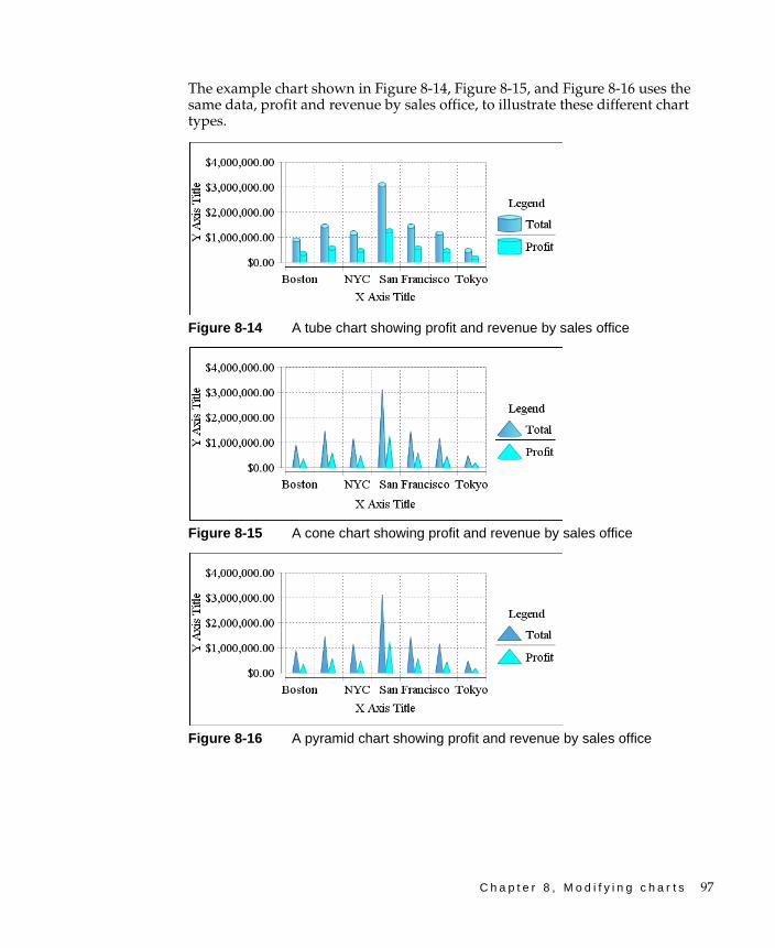
C h a p t e r 8 , M o d i f y i n g c h a r t s 97
The example chart shown in Figure 8-14, Figure 8-15, and Figure 8-16 uses the same data, profit and revenue by sales office, to illustrate these different chart types.
Figure 8-14 A tube chart showing profit and revenue by sales office
Figure 8-15 A cone chart showing profit and revenue by sales office
Figure 8-16 A pyramid chart showing profit and revenue by sales office
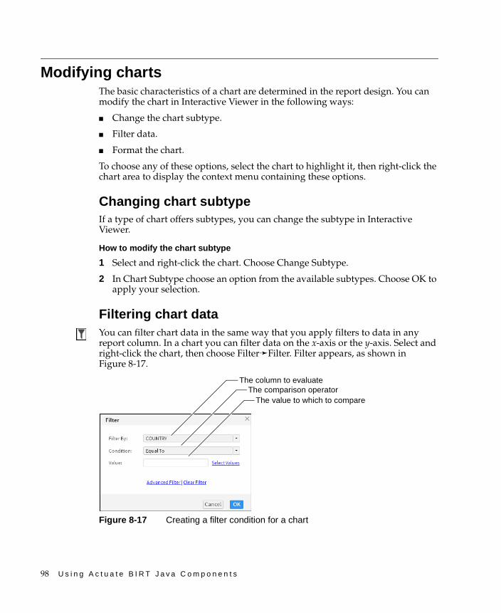
98 U s i n g A c t u a t e B I R T J a v a C o m p o n e n t s
Modifying chartsThe basic characteristics of a chart are determined in the report design. You can modify the chart in Interactive Viewer in the following ways:
■ Change the chart subtype.
■ Filter data.
■ Format the chart.
To choose any of these options, select the chart to highlight it, then right-click the chart area to display the context menu containing these options.
Changing chart subtypeIf a type of chart offers subtypes, you can change the subtype in Interactive Viewer.
How to modify the chart subtype
1 Select and right-click the chart. Choose Change Subtype.
2 In Chart Subtype choose an option from the available subtypes. Choose OK to apply your selection.
Filtering chart dataYou can filter chart data in the same way that you apply filters to data in any report column. In a chart you can filter data on the x-axis or the y-axis. Select and right-click the chart, then choose Filter➛Filter. Filter appears, as shown in Figure 8-17.
Figure 8-17 Creating a filter condition for a chart
The value to which to compareThe comparison operator
The column to evaluate
C h a p t e r 8 , M o d i f y i n g c h a r t s 99
Complete the steps to create one or more filter conditions as described in a previous section of this document, based on which data is displayed on the axes of the chart.
When filtering a Gantt chart, the value set as the task label and the value by which legend items are grouped can impact the filtered data displayed. For example, in a Gantt chart displaying order processing times, if the task label is set to Country and the legend is grouped by product line, specifying a filter on the country column appears to display data for the selected country. However, because the tasks are aggregated by product line, each bar in the Gantt chart contains data aggregated by product line for several countries, even though the task label displays the name of a single country specified in the filter condition. So although the filtered data is accurate, it can appear confusing to the user.
Formatting a chartCharts include many different visual elements, as shown in Figure 8-18. You can customize the appearance of many of these elements using Interactive Viewer. To clarify the presentation of data, or to create a more pleasing composition, you can rearrange the layout of the chart. Some of the formatting for a chart, such as the colors of the bars in a bar chart and the background color of the chart, are defined in the original report, and cannot be modified. When viewing the report you can modify the fonts and font sizes of the chart title and axis labels, and the height and width of the chart. You can hide axis labels, place labels at an angle relative to the axis, and hide the legend or determine where to display the legend in relation to the chart. Depending on the type of chart you are working with, you can also transpose the axes in some cases.
Figure 8-18 displays the elements of a basic bar chart that you can format using Interactive Viewer. In this example, the category series consists of a set of regions, and the value series consists of a set of sales figure values.
As mentioned in an earlier section, a chart organizes data points into value sets called series. Series can be of two types—a category series and a value series. The category series typically determines what text, numbers, or dates you see on the x-axis. The value series typically determines the text, numbers, or dates on the y-axis. A value axis positions data relative to the axis marks. The value of a data point determines where it appears on a value axis. You do not plot text on a value axis. In most charts with axes, the x-axis is the category axis, and the y-axis is a value axis.
The plotting options available for the x- and y-axes can differ in name and function, depending on the chart type. For example, when you modify a meter chart, which has no axes, you define the position of a needle on the dial instead of defining the y-axis. When you modify a pie chart, you define the size of the slices instead of the y-axis.
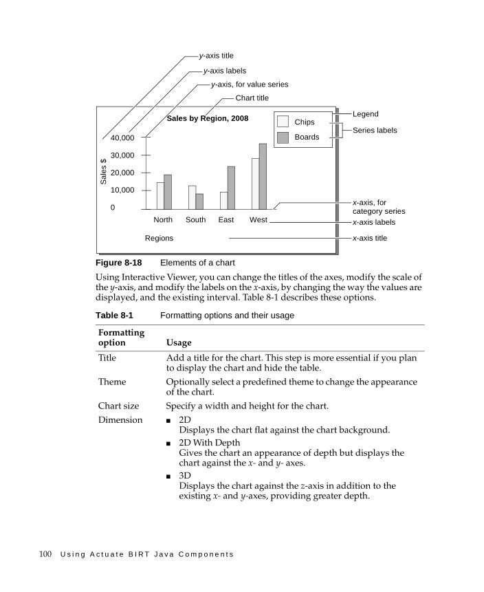
100 U s i n g A c t u a t e B I R T J a v a C o m p o n e n t s
Figure 8-18 Elements of a chart
Using Interactive Viewer, you can change the titles of the axes, modify the scale of the y-axis, and modify the labels on the x-axis, by changing the way the values are displayed, and the existing interval. Table 8-1 describes these options.
Table 8-1 Formatting options and their usage
Formatting option Usage
Title Add a title for the chart. This step is more essential if you plan to display the chart and hide the table.
Theme Optionally select a predefined theme to change the appearance of the chart.
Chart size Specify a width and height for the chart.
Dimension ■ 2DDisplays the chart flat against the chart background.
■ 2D With DepthGives the chart an appearance of depth but displays the chart against the x- and y- axes.
■ 3DDisplays the chart against the z-axis in addition to the existing x- and y-axes, providing greater depth.
Sales by Region, 2008 Chips
Boards40,000
30,000
20,000
10,000
0
Regions
North South East West
Sal
es $
Chart title
x-axis title
x-axis labels
y-axis, for value series
x-axis, for category series
y-axis labels
y-axis title
Legend
Series labels
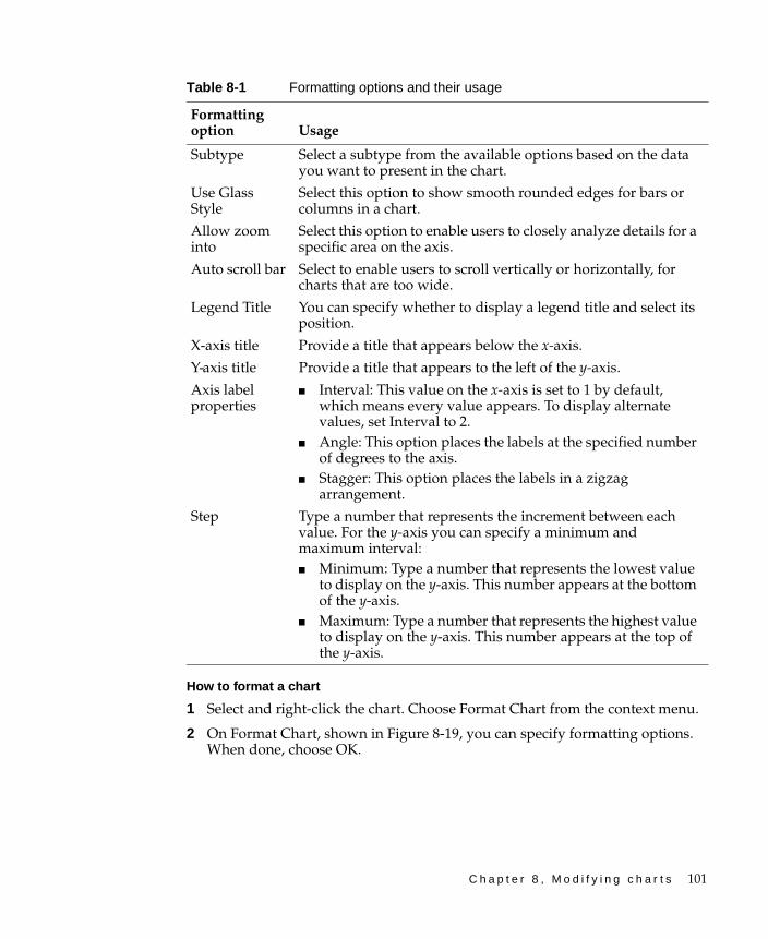
C h a p t e r 8 , M o d i f y i n g c h a r t s 101
How to format a chart
1 Select and right-click the chart. Choose Format Chart from the context menu.
2 On Format Chart, shown in Figure 8-19, you can specify formatting options. When done, choose OK.
Subtype Select a subtype from the available options based on the data you want to present in the chart.
Use Glass Style
Select this option to show smooth rounded edges for bars or columns in a chart.
Allow zoom into
Select this option to enable users to closely analyze details for a specific area on the axis.
Auto scroll bar Select to enable users to scroll vertically or horizontally, for charts that are too wide.
Legend Title You can specify whether to display a legend title and select its position.
X-axis title Provide a title that appears below the x-axis.
Y-axis title Provide a title that appears to the left of the y-axis.
Axis label properties
■ Interval: This value on the x-axis is set to 1 by default, which means every value appears. To display alternate values, set Interval to 2.
■ Angle: This option places the labels at the specified number of degrees to the axis.
■ Stagger: This option places the labels in a zigzag arrangement.
Step Type a number that represents the increment between each value. For the y-axis you can specify a minimum and maximum interval:■ Minimum: Type a number that represents the lowest value
to display on the y-axis. This number appears at the bottom of the y-axis.
■ Maximum: Type a number that represents the highest value to display on the y-axis. This number appears at the top of the y-axis.
Table 8-1 Formatting options and their usage
Formatting option Usage
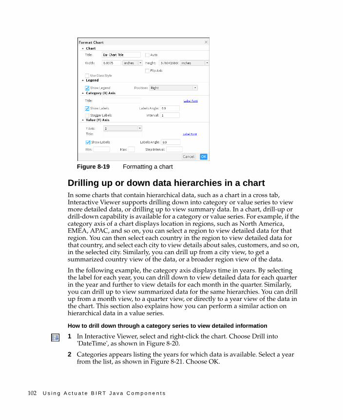
102 U s i n g A c t u a t e B I R T J a v a C o m p o n e n t s
Figure 8-19 Formatting a chart
Drilling up or down data hierarchies in a chartIn some charts that contain hierarchical data, such as a chart in a cross tab, Interactive Viewer supports drilling down into category or value series to view more detailed data, or drilling up to view summary data. In a chart, drill-up or drill-down capability is available for a category or value series. For example, if the category axis of a chart displays location in regions, such as North America, EMEA, APAC, and so on, you can select a region to view detailed data for that region. You can then select each country in the region to view detailed data for that country, and select each city to view details about sales, customers, and so on, in the selected city. Similarly, you can drill up from a city view, to get a summarized country view of the data, or a broader region view of the data.
In the following example, the category axis displays time in years. By selecting the label for each year, you can drill down to view detailed data for each quarter in the year and further to view details for each month in the quarter. Similarly, you can drill up to view summarized data for the same hierarchies. You can drill up from a month view, to a quarter view, or directly to a year view of the data in the chart. This section also explains how you can perform a similar action on hierarchical data in a value series.
How to drill down through a category series to view detailed information
1 In Interactive Viewer, select and right-click the chart. Choose Drill into 'DateTime', as shown in Figure 8-20.
2 Categories appears listing the years for which data is available. Select a year from the list, as shown in Figure 8-21. Choose OK.
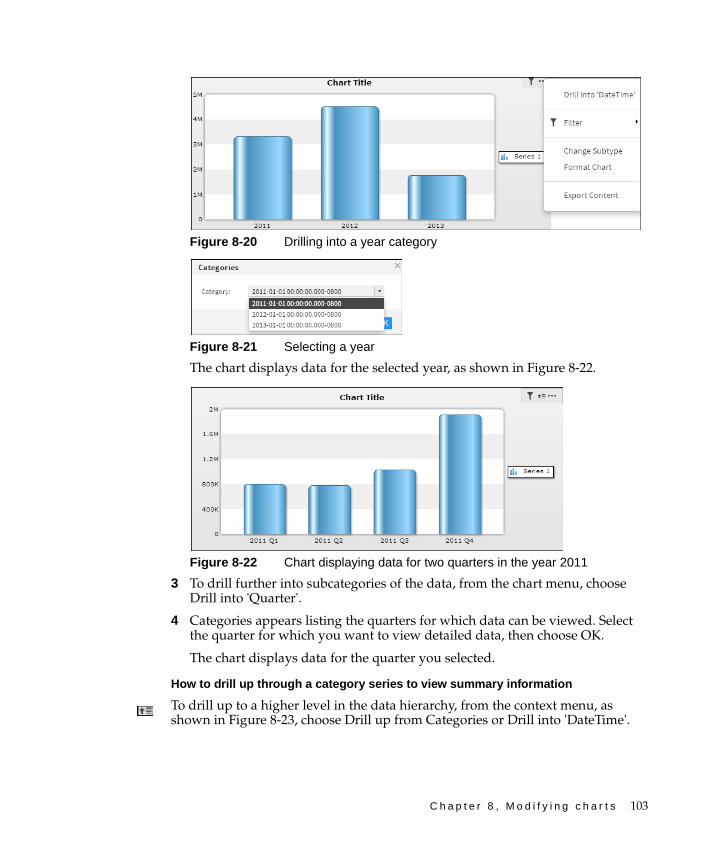
C h a p t e r 8 , M o d i f y i n g c h a r t s 103
Figure 8-20 Drilling into a year category
Figure 8-21 Selecting a year
The chart displays data for the selected year, as shown in Figure 8-22.
Figure 8-22 Chart displaying data for two quarters in the year 2011
3 To drill further into subcategories of the data, from the chart menu, choose Drill into 'Quarter'.
4 Categories appears listing the quarters for which data can be viewed. Select the quarter for which you want to view detailed data, then choose OK.
The chart displays data for the quarter you selected.
How to drill up through a category series to view summary information
To drill up to a higher level in the data hierarchy, from the context menu, as shown in Figure 8-23, choose Drill up from Categories or Drill into 'DateTime'.
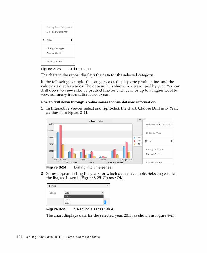
104 U s i n g A c t u a t e B I R T J a v a C o m p o n e n t s
Figure 8-23 Drill-up menu
The chart in the report displays the data for the selected category.
In the following example, the category axis displays the product line, and the value axis displays sales. The data in the value series is grouped by year. You can drill down to view sales by product line for each year, or up to a higher level to view summary information across years.
How to drill down through a value series to view detailed information
1 In Interactive Viewer, select and right-click the chart. Choose Drill into 'Year,' as shown in Figure 8-24.
Figure 8-24 Drilling into time series
2 Series appears listing the years for which data is available. Select a year from the list, as shown in Figure 8-25. Choose OK.
Figure 8-25 Selecting a series value
The chart displays data for the selected year, 2011, as shown in Figure 8-26.
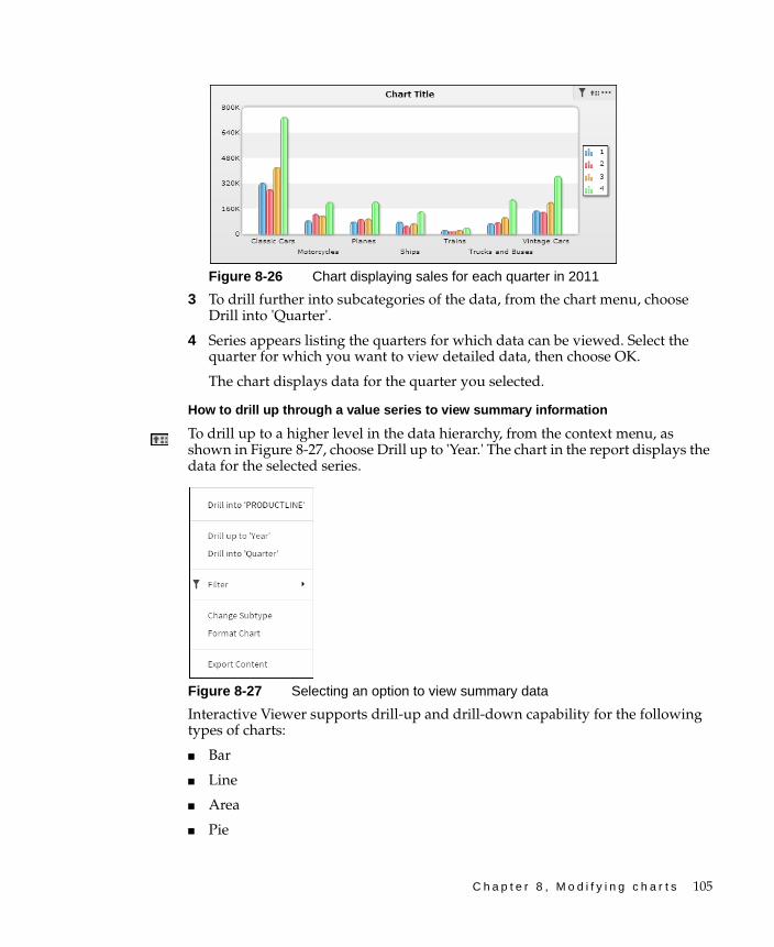
C h a p t e r 8 , M o d i f y i n g c h a r t s 105
Figure 8-26 Chart displaying sales for each quarter in 2011
3 To drill further into subcategories of the data, from the chart menu, choose Drill into 'Quarter'.
4 Series appears listing the quarters for which data can be viewed. Select the quarter for which you want to view detailed data, then choose OK.
The chart displays data for the quarter you selected.
How to drill up through a value series to view summary information
To drill up to a higher level in the data hierarchy, from the context menu, as shown in Figure 8-27, choose Drill up to 'Year.' The chart in the report displays the data for the selected series.
Figure 8-27 Selecting an option to view summary data
Interactive Viewer supports drill-up and drill-down capability for the following types of charts:
■ Bar
■ Line
■ Area
■ Pie
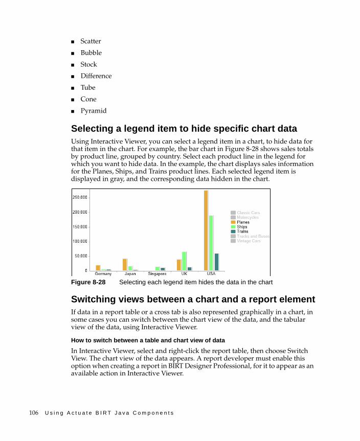
106 U s i n g A c t u a t e B I R T J a v a C o m p o n e n t s
■ Scatter
■ Bubble
■ Stock
■ Difference
■ Tube
■ Cone
■ Pyramid
Selecting a legend item to hide specific chart dataUsing Interactive Viewer, you can select a legend item in a chart, to hide data for that item in the chart. For example, the bar chart in Figure 8-28 shows sales totals by product line, grouped by country. Select each product line in the legend for which you want to hide data. In the example, the chart displays sales information for the Planes, Ships, and Trains product lines. Each selected legend item is displayed in gray, and the corresponding data hidden in the chart.
Figure 8-28 Selecting each legend item hides the data in the chart
Switching views between a chart and a report elementIf data in a report table or a cross tab is also represented graphically in a chart, in some cases you can switch between the chart view of the data, and the tabular view of the data, using Interactive Viewer.
How to switch between a table and chart view of data
In Interactive Viewer, select and right-click the report table, then choose Switch View. The chart view of the data appears. A report developer must enable this option when creating a report in BIRT Designer Professional, for it to appear as an available action in Interactive Viewer.

C h a p t e r 8 , M o d i f y i n g c h a r t s 107
If you are working with a cross tab, choose Switch View from the context menu. You can also further analyze the data in a cross tab by choosing the Analyze option from the context menu. The cross tab appears in Interactive Crosstabs if you have purchased this licensed option.
Similarly, to switch back to the table view, select and right-click the chart, then choose Switch View. The table or cross tab view of the data appears.
Using the timeline optionsIn Interactive viewer, if your chart contains a time range selector or a time line slider bar you can view specific time intervals in area, bar, column, difference, line, scatter, and stock charts. Figure 8-29 shows a chart displaying the time range selector and bottom slider.
Figure 8-29 Enabling the timeline option in a column chart
The time range selector appears below the chart title and enables you to view details in small time intervals, year to date, one year, in addition to all the values displayed in the chart. The time range slider appears at the bottom of the chart and enables you to select a time period by sliding a bar to the beginning or end of the time period. When the category is a time field, you can select the time range selector and bottom slider.

108 U s i n g A c t u a t e B I R T J a v a C o m p o n e n t s
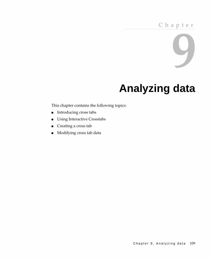
C h a p t e r 9 , A n a l y z i n g d a t a 109
C h a p t e r
9Chapter 9Analyzing data
This chapter contains the following topics:
■ Introducing cross tabs
■ Using Interactive Crosstabs
■ Creating a cross tab
■ Modifying cross tab data
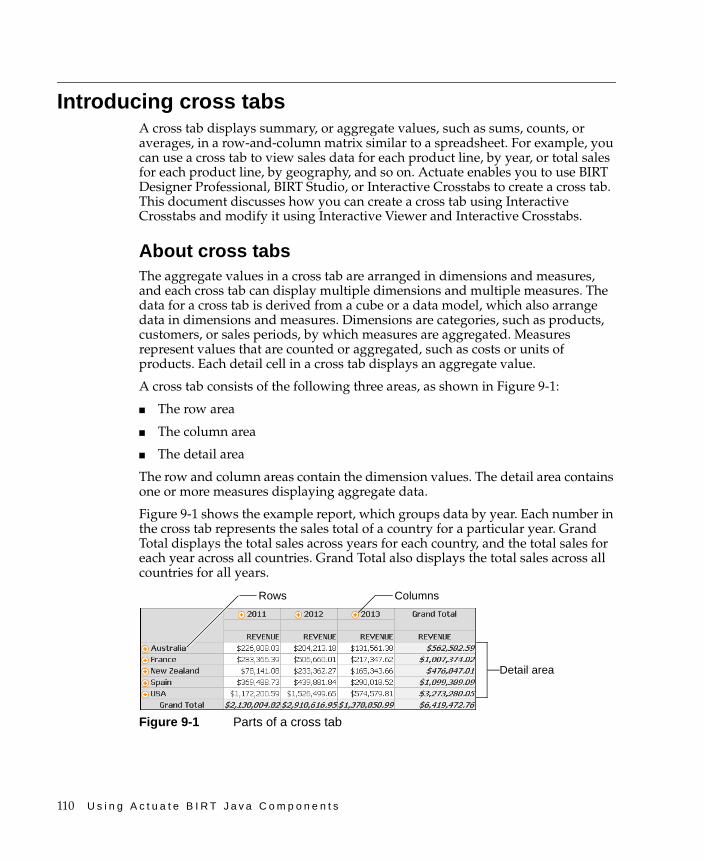
110 U s i n g A c t u a t e B I R T J a v a C o m p o n e n t s
Introducing cross tabsA cross tab displays summary, or aggregate values, such as sums, counts, or averages, in a row-and-column matrix similar to a spreadsheet. For example, you can use a cross tab to view sales data for each product line, by year, or total sales for each product line, by geography, and so on. Actuate enables you to use BIRT Designer Professional, BIRT Studio, or Interactive Crosstabs to create a cross tab. This document discusses how you can create a cross tab using Interactive Crosstabs and modify it using Interactive Viewer and Interactive Crosstabs.
About cross tabsThe aggregate values in a cross tab are arranged in dimensions and measures, and each cross tab can display multiple dimensions and multiple measures. The data for a cross tab is derived from a cube or a data model, which also arrange data in dimensions and measures. Dimensions are categories, such as products, customers, or sales periods, by which measures are aggregated. Measures represent values that are counted or aggregated, such as costs or units of products. Each detail cell in a cross tab displays an aggregate value.
A cross tab consists of the following three areas, as shown in Figure 9-1:
■ The row area
■ The column area
■ The detail area
The row and column areas contain the dimension values. The detail area contains one or more measures displaying aggregate data.
Figure 9-1 shows the example report, which groups data by year. Each number in the cross tab represents the sales total of a country for a particular year. Grand Total displays the total sales across years for each country, and the total sales for each year across all countries. Grand Total also displays the total sales across all countries for all years.
Figure 9-1 Parts of a cross tab
Detail area
Rows Columns
C h a p t e r 9 , A n a l y z i n g d a t a 111
Obtaining data for a cross tabIn BIRT iHub and later releases, a cross tab obtains data from a BIRT data object containing a cube or data model. A cube is a multidimensional data structure optimized for analysis. A data model consists of several data sets in a data object linked by joins. Both cubes and data models organize data in dimensions, measures, and attributes. Dimensions can contain multilevel hierarchies, enabling users to drill down to view detailed information or drill up to view summary information for each level within the hierarchy. For example, a time dimension can provide the ability to display data by day, week, month, quarter, or year. The time dimension also supports storing data in the time periods a data object developer specifies. A geographical dimension can provide the ability to display data by region, country, state, or city, enabling the user to view high level summary information or details for each dimension level.
Query optimization in a data model offers better performance than a cube. A data model also provides you with more flexibility in your choice of dimensions and measures.
Using Interactive CrosstabsUsing Interactive Crosstabs, you can add, remove, reorganize, and customize the data in a cross tab to examine relationships and trends. Interactive cross tabs provides you with the ability to drill down into dimension levels to display detail data, drill up to display summary data, filter, group, and sort data in a cross tab, perform calculations, create aggregate data, and display cross tab data in a grid or in a chart. These actions enable you to gather business intelligence information such as a product’s sales over a period of time, which products sell more or less by geography, how many units of a product shipped in a specific month, and so on.
You can launch Interactive Crosstabs in the following ways:
■ Navigate to a BIRT data object store (.data) file containing a cube or data model in the iHub volume. Choose the file and select an available cube or data model. Interactive Crosstabs launches displaying the selected data source. You can now create a cross tab.
■ Obtain a URL link from your report developer or system administrator to supported BIRT cube view (.cubeview) files or BIRT data object store (.data) files containing a cube or data model. In Interactive Crosstabs, you can modify the BIRT cube view file or create a cross tab using the BIRT data object store (.data) file.
■ Launch Interactive Crosstabs when viewing a cross tab in other applications such as BIRT Studio or Interactive Viewer. You can view and modify cross tabs
112 U s i n g A c t u a t e B I R T J a v a C o m p o n e n t s
in BIRT cube view (.cubeview) files, BIRT design (.rptdesign) files, and BIRT document (.rptdocument) files.
■ Use Actuate JavaScript API to access Interactive Crosstabs embedded in a web page by a developer. For more information see Actuate BIRT Java Components Developer Guide.
When you create a cross tab either in BIRT Designer Professional, BIRT Studio, or Interactive Crosstabs, you can use Interactive Viewer or Interactive Crosstabs to modify the cross tab. You can use either application to format cross tab data to change the appearance of specific values, display detail information for data values to view summary information at a glance, or modify a chart. You can also export cross tab content to other formats such as Excel, Word, PowerPoint, PostScript, PDF or XHTML. If you save a cross tab using Interactive Crosstabs or Interactive Viewer, you can save the cross tab as a BIRT cube view (.cubeview) file, a BIRT design (.rptdesign) file, or a BIRT document (.rptdocument) file. If you open a cross tab in BIRT Studio and modify it using Interactive Crosstabs, you must save the cross tab as a BIRT design file. You can print a cross tab using Interactive Viewer.
Creating a cross tabTo create a cross tab, you need access to a BIRT data object containing a cube or data model in the volume. When you populate a cross tab in Interactive Crosstabs, the default view available is the grid or tabular view. You can switch to chart view to display the same data graphically in a chart based on HTML5 technology. The default chart type is a column chart. You can change this to a chart type more suited for the data in your cross tab as described in later sections of this document.
When you create a cross tab, you choose the dimension, attribute, and measure fields to display. For dimension fields containing date-and-time data, you also specify a grouping interval. For measure fields, you specify a function based on which the aggregate value in each detail cell is calculated. You can also specify whether to display subtotals or grand totals, or both, and the location.
How to create a cross tab using Interactive Crosstabs
1 Obtain the Visualization Platform URL and login information from your system administrator. Login to Visualization Platform.
2 In the volume, in the navigation pane select the Resources folder. Select a BIRT data object store (.data) file containing a cube or data model to use for the cross tab. The example in this procedure uses the sample data object store file, Classic Models.data.
3 Select Data appears. In Available Data, select a cube or data model from the list. Figure 9-2 shows the selection of Data Model.
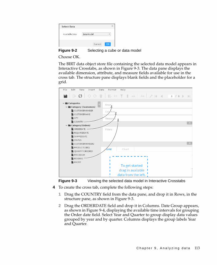
C h a p t e r 9 , A n a l y z i n g d a t a 113
Figure 9-2 Selecting a cube or data model
Choose OK.
The BIRT data object store file containing the selected data model appears in Interactive Crosstabs, as shown in Figure 9-3. The data pane displays the available dimension, attribute, and measure fields available for use in the cross tab. The structure pane displays blank fields and the placeholder for a grid.
Figure 9-3 Viewing the selected data model in Interactive Crosstabs
4 To create the cross tab, complete the following steps:
1 Drag the COUNTRY field from the data pane, and drop it in Rows, in the structure pane, as shown in Figure 9-3.
2 Drag the ORDERDATE field and drop it in Columns. Date Group appears, as shown in Figure 9-4, displaying the available time intervals for grouping the Order date field. Select Year and Quarter to group display data values grouped by year and by quarter. Columns displays the group labels Year and Quarter.
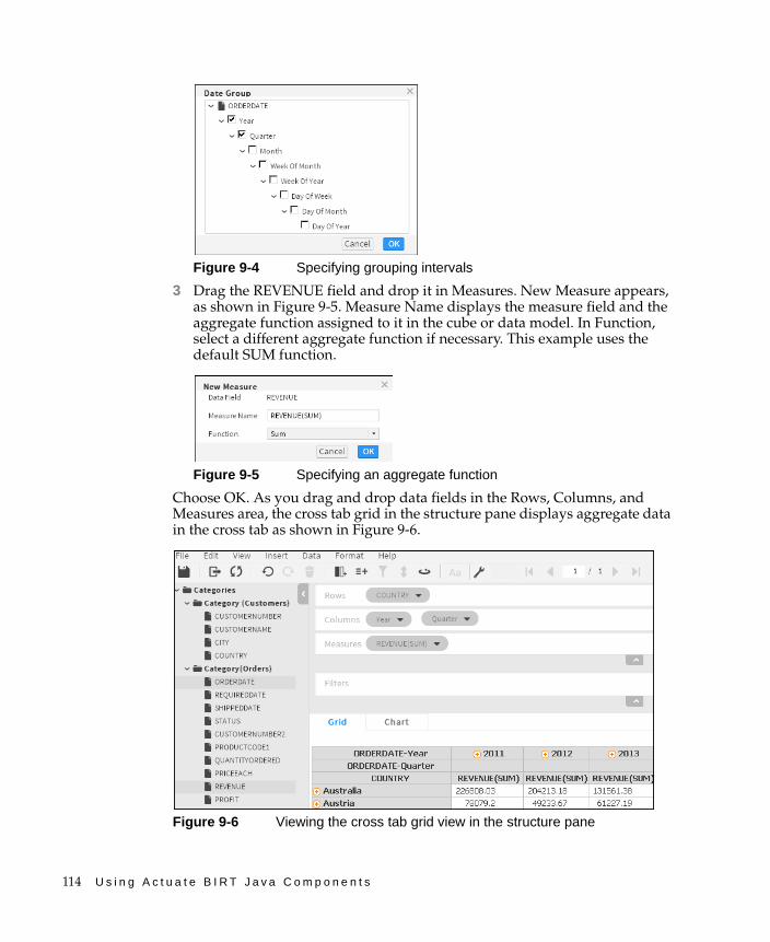
114 U s i n g A c t u a t e B I R T J a v a C o m p o n e n t s
Figure 9-4 Specifying grouping intervals
3 Drag the REVENUE field and drop it in Measures. New Measure appears, as shown in Figure 9-5. Measure Name displays the measure field and the aggregate function assigned to it in the cube or data model. In Function, select a different aggregate function if necessary. This example uses the default SUM function.
Figure 9-5 Specifying an aggregate function
Choose OK. As you drag and drop data fields in the Rows, Columns, and Measures area, the cross tab grid in the structure pane displays aggregate data in the cross tab as shown in Figure 9-6.
Figure 9-6 Viewing the cross tab grid view in the structure pane
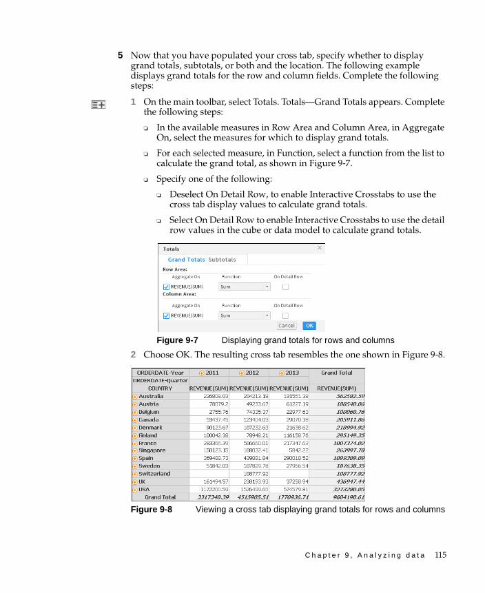
C h a p t e r 9 , A n a l y z i n g d a t a 115
5 Now that you have populated your cross tab, specify whether to display grand totals, subtotals, or both and the location. The following example displays grand totals for the row and column fields. Complete the following steps:
1 On the main toolbar, select Totals. Totals—Grand Totals appears. Complete the following steps:
❏ In the available measures in Row Area and Column Area, in Aggregate On, select the measures for which to display grand totals.
❏ For each selected measure, in Function, select a function from the list to calculate the grand total, as shown in Figure 9-7.
❏ Specify one of the following:
❏ Deselect On Detail Row, to enable Interactive Crosstabs to use the cross tab display values to calculate grand totals.
❏ Select On Detail Row to enable Interactive Crosstabs to use the detail row values in the cube or data model to calculate grand totals.
Figure 9-7 Displaying grand totals for rows and columns
2 Choose OK. The resulting cross tab resembles the one shown in Figure 9-8.
Figure 9-8 Viewing a cross tab displaying grand totals for rows and columns
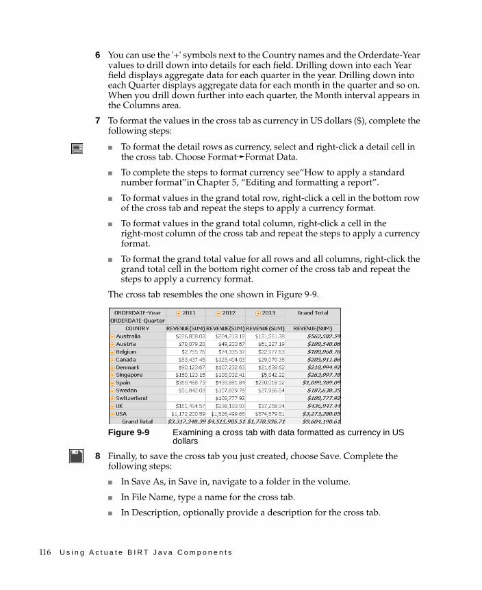
116 U s i n g A c t u a t e B I R T J a v a C o m p o n e n t s
6 You can use the '+' symbols next to the Country names and the Orderdate-Year values to drill down into details for each field. Drilling down into each Year field displays aggregate data for each quarter in the year. Drilling down into each Quarter displays aggregate data for each month in the quarter and so on. When you drill down further into each quarter, the Month interval appears in the Columns area.
7 To format the values in the cross tab as currency in US dollars ($), complete the following steps:
■ To format the detail rows as currency, select and right-click a detail cell in the cross tab. Choose Format➛Format Data.
■ To complete the steps to format currency see“How to apply a standard number format”in Chapter 5, “Editing and formatting a report”.
■ To format values in the grand total row, right-click a cell in the bottom row of the cross tab and repeat the steps to apply a currency format.
■ To format values in the grand total column, right-click a cell in the right-most column of the cross tab and repeat the steps to apply a currency format.
■ To format the grand total value for all rows and all columns, right-click the grand total cell in the bottom right corner of the cross tab and repeat the steps to apply a currency format.
The cross tab resembles the one shown in Figure 9-9.
Figure 9-9 Examining a cross tab with data formatted as currency in US dollars
8 Finally, to save the cross tab you just created, choose Save. Complete the following steps:
■ In Save As, in Save in, navigate to a folder in the volume.
■ In File Name, type a name for the cross tab.
■ In Description, optionally provide a description for the cross tab.
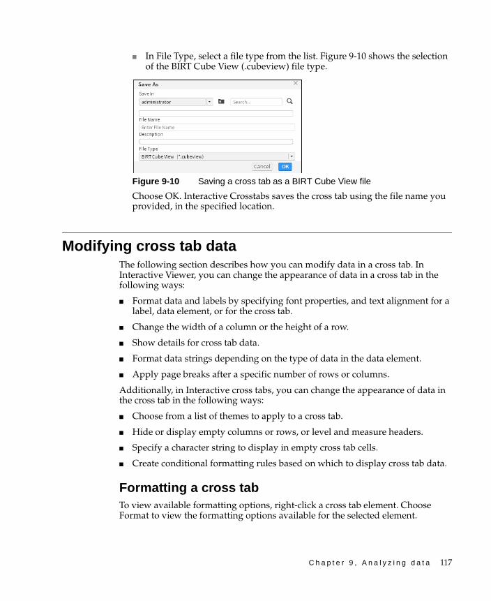
C h a p t e r 9 , A n a l y z i n g d a t a 117
■ In File Type, select a file type from the list. Figure 9-10 shows the selection of the BIRT Cube View (.cubeview) file type.
Figure 9-10 Saving a cross tab as a BIRT Cube View file
Choose OK. Interactive Crosstabs saves the cross tab using the file name you provided, in the specified location.
Modifying cross tab dataThe following section describes how you can modify data in a cross tab. In Interactive Viewer, you can change the appearance of data in a cross tab in the following ways:
■ Format data and labels by specifying font properties, and text alignment for a label, data element, or for the cross tab.
■ Change the width of a column or the height of a row.
■ Show details for cross tab data.
■ Format data strings depending on the type of data in the data element.
■ Apply page breaks after a specific number of rows or columns.
Additionally, in Interactive cross tabs, you can change the appearance of data in the cross tab in the following ways:
■ Choose from a list of themes to apply to a cross tab.
■ Hide or display empty columns or rows, or level and measure headers.
■ Specify a character string to display in empty cross tab cells.
■ Create conditional formatting rules based on which to display cross tab data.
Formatting a cross tabTo view available formatting options, right-click a cross tab element. Choose Format to view the formatting options available for the selected element.
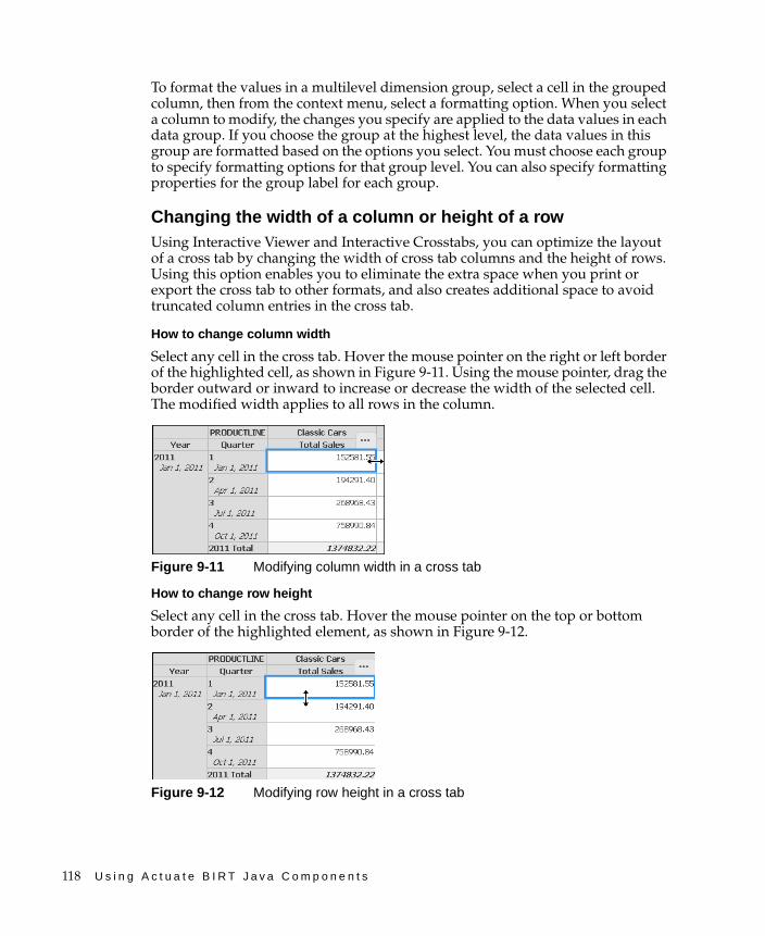
118 U s i n g A c t u a t e B I R T J a v a C o m p o n e n t s
To format the values in a multilevel dimension group, select a cell in the grouped column, then from the context menu, select a formatting option. When you select a column to modify, the changes you specify are applied to the data values in each data group. If you choose the group at the highest level, the data values in this group are formatted based on the options you select. You must choose each group to specify formatting options for that group level. You can also specify formatting properties for the group label for each group.
Changing the width of a column or height of a rowUsing Interactive Viewer and Interactive Crosstabs, you can optimize the layout of a cross tab by changing the width of cross tab columns and the height of rows. Using this option enables you to eliminate the extra space when you print or export the cross tab to other formats, and also creates additional space to avoid truncated column entries in the cross tab.
How to change column width
Select any cell in the cross tab. Hover the mouse pointer on the right or left border of the highlighted cell, as shown in Figure 9-11. Using the mouse pointer, drag the border outward or inward to increase or decrease the width of the selected cell. The modified width applies to all rows in the column.
Figure 9-11 Modifying column width in a cross tab
How to change row height
Select any cell in the cross tab. Hover the mouse pointer on the top or bottom border of the highlighted element, as shown in Figure 9-12.
Figure 9-12 Modifying row height in a cross tab

C h a p t e r 9 , A n a l y z i n g d a t a 119
Using the mouse pointer, drag the border up or down to increase or decrease the height of the selected element. The modified height applies to the entire row.
Using themesYou can modify themes in a cross tab using Interactive Crosstabs. Themes are optional. Interactive Crosstabs provides a set of predefined themes, but you can also use custom themes, if they exist. A developer creates a theme library, a library (.rptlibrary) file, using BIRT Designer Professional, and publishes it to the Resources folder in the Encyclopedia volume, for example:
/Resources/ThemesReportItems3.rptlibrary
A library can include multiple themes if the library developer chooses to provide users with different style options to apply to cross tabs.
How to specify a theme for a cross tab
In Interactive Crosstabs, choose Format➛Theme. Select a theme from the menu that appears.
A cross tab displaying the Grayscale theme is shown in Figure 9-13.
Figure 9-13 Viewing the grayscale theme in a cross tab
Viewing details for cross tab dataDisplaying detail tooltip information is specifically useful if you are analyzing data in a large cross tab where you cannot simultaneously view the column heading, row heading, and data cell in your browser window.
To view details, right-click any cell in the detail area, and choose Show Detail Tooltip. A tooltip displays the column and row-level details, the measure value, and which aggregate function applies for the selected cell, as shown in Figure 9-14.
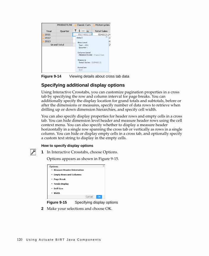
120 U s i n g A c t u a t e B I R T J a v a C o m p o n e n t s
Figure 9-14 Viewing details about cross tab data
Specifying additional display optionsUsing Interactive Crosstabs, you can customize pagination properties in a cross tab by specifying the row and column interval for page breaks. You can additionally specify the display location for grand totals and subtotals, before or after the dimensions or measures, specify number of data rows to retrieve when drilling up or down dimension hierarchies, and specify cell width.
You can also specify display properties for header rows and empty cells in a cross tab. You can hide dimension level header and measure header rows using the cell context menu. You can also specify whether to display a measure header horizontally in a single row spanning the cross tab or vertically as rows in a single column. You can hide or display empty cells in a cross tab, and optionally specify a custom text string to display in the empty cells.
How to specify display options
1 In Interactive Crosstabs, choose Options.
Options appears as shown in Figure 9-15.
Figure 9-15 Specifying display options
2 Make your selections and choose OK.

C h a p t e r 9 , A n a l y z i n g d a t a 121
Organizing data in a cross tabUsing Interactive Crosstabs you can organize cross tab data in the following ways:
■ Sort data in a column in ascending or descending order.
■ Add, remove, or reorder attribute, dimension, and measure columns.
■ Pivot the cross tab, which transposes the columns and rows axes.
■ Drill down to display details or drill up to display summary information.
The following section describes these actions in more detail.
Sorting data in a cross tabYou can sort data in a cross tab to display the content in a meaningful order. A sales cross tab is more useful if it presents sales figures from highest to lowest, or the reverse, if you want to see lowest-to-highest performers. The default sort order in a cross tab displays data sorted by dimension values. The column-and-row heading values, which are dimensions, appear in ascending order.
Compare the cross tabs in Figure 9-16. The cross tab on the left displays sales revenues for products by alphabetically sorted country names. The cross tab on the right displays the same data, with sales revenues sorted from the highest to lowest in the grand total column.
Figure 9-16 Comparing cross tabs that contain sorted data
Interactive Crosstabs supports sorting values in a column or row. For dimension-level groups, you can specify a sort order for fields in the hierarchy. For example, you can specify an ascending or descending sort order for the time period hierarchy of year and quarter, as shown in Figure 9-17.
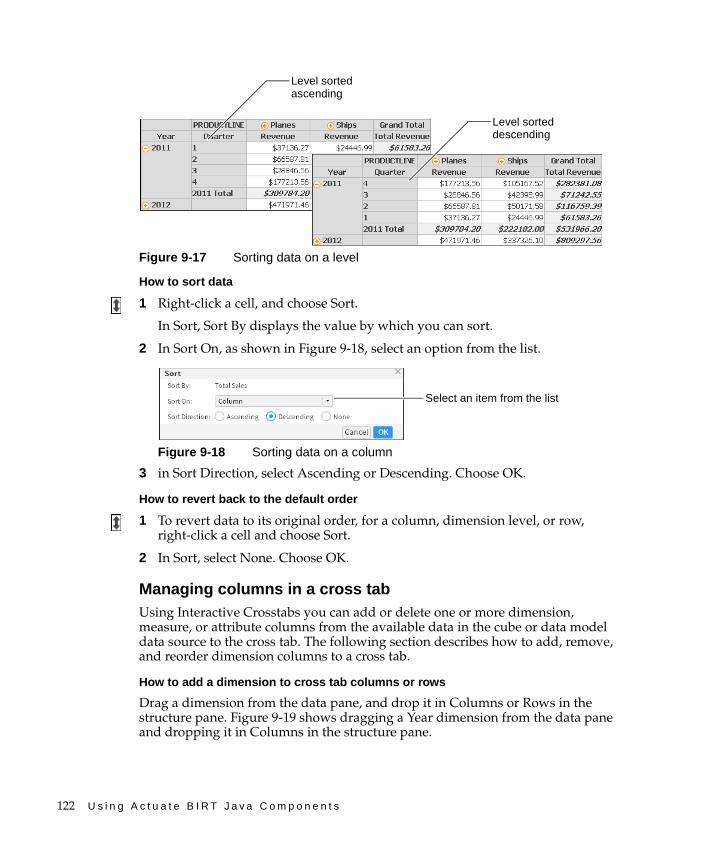
122 U s i n g A c t u a t e B I R T J a v a C o m p o n e n t s
Figure 9-17 Sorting data on a level
How to sort data
1 Right-click a cell, and choose Sort.
In Sort, Sort By displays the value by which you can sort.
2 In Sort On, as shown in Figure 9-18, select an option from the list.
Figure 9-18 Sorting data on a column
3 in Sort Direction, select Ascending or Descending. Choose OK.
How to revert back to the default order
1 To revert data to its original order, for a column, dimension level, or row, right-click a cell and choose Sort.
2 In Sort, select None. Choose OK.
Managing columns in a cross tabUsing Interactive Crosstabs you can add or delete one or more dimension, measure, or attribute columns from the available data in the cube or data model data source to the cross tab. The following section describes how to add, remove, and reorder dimension columns to a cross tab.
How to add a dimension to cross tab columns or rows
Drag a dimension from the data pane, and drop it in Columns or Rows in the structure pane. Figure 9-19 shows dragging a Year dimension from the data pane and dropping it in Columns in the structure pane.
Level sorted ascending
Level sorted descending
Select an item from the list
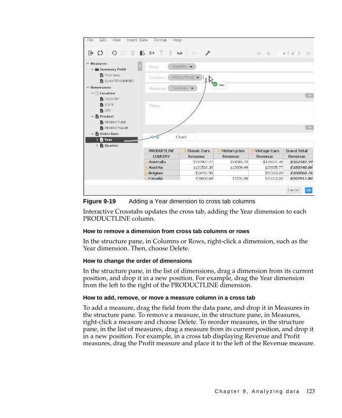
C h a p t e r 9 , A n a l y z i n g d a t a 123
Figure 9-19 Adding a Year dimension to cross tab columns
Interactive Crosstabs updates the cross tab, adding the Year dimension to each PRODUCTLINE column.
How to remove a dimension from cross tab columns or rows
In the structure pane, in Columns or Rows, right-click a dimension, such as the Year dimension. Then, choose Delete.
How to change the order of dimensions
In the structure pane, in the list of dimensions, drag a dimension from its current position, and drop it in a new position. For example, drag the Year dimension from the left to the right of the PRODUCTLINE dimension.
How to add, remove, or move a measure column in a cross tab
To add a measure, drag the field from the data pane, and drop it in Measures in the structure pane. To remove a measure, in the structure pane, in Measures, right-click a measure and choose Delete. To reorder measures, in the structure pane, in the list of measures, drag a measure from its current position, and drop it in a new position. For example, in a cross tab displaying Revenue and Profit measures, drag the Profit measure and place it to the left of the Revenue measure.
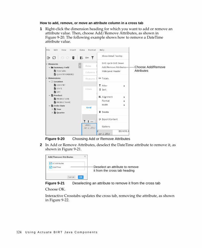
124 U s i n g A c t u a t e B I R T J a v a C o m p o n e n t s
How to add, remove, or move an attribute column in a cross tab
1 Right-click the dimension heading for which you want to add or remove an attribute value. Then, choose Add/Remove Attributes, as shown in Figure 9-20. The following example shows how to remove a DateTime attribute value.
Figure 9-20 Choosing Add or Remove Attributes
2 In Add or Remove Attributes, deselect the DateTime attribute to remove it, as shown in Figure 9-21.
Figure 9-21 Deselecting an attribute to remove it from the cross tab
Choose OK.
Interactive Crosstabs updates the cross tab, removing the attribute, as shown in Figure 9-22.
Choose Add/Remove Attributes
Deselect an attribute to remove it from the cross tab heading
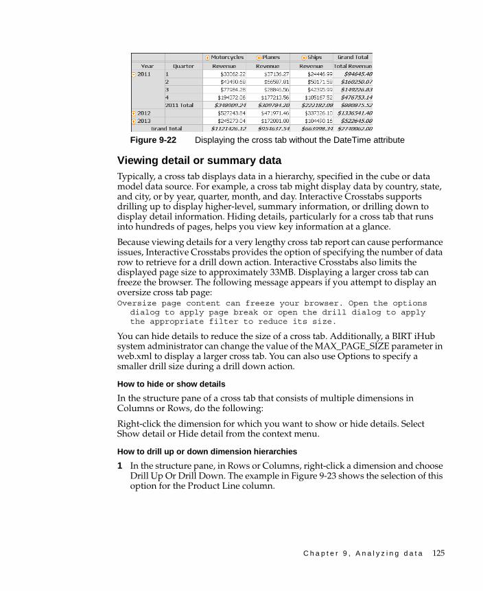
C h a p t e r 9 , A n a l y z i n g d a t a 125
Figure 9-22 Displaying the cross tab without the DateTime attribute
Viewing detail or summary dataTypically, a cross tab displays data in a hierarchy, specified in the cube or data model data source. For example, a cross tab might display data by country, state, and city, or by year, quarter, month, and day. Interactive Crosstabs supports drilling up to display higher-level, summary information, or drilling down to display detail information. Hiding details, particularly for a cross tab that runs into hundreds of pages, helps you view key information at a glance.
Because viewing details for a very lengthy cross tab report can cause performance issues, Interactive Crosstabs provides the option of specifying the number of data row to retrieve for a drill down action. Interactive Crosstabs also limits the displayed page size to approximately 33MB. Displaying a larger cross tab can freeze the browser. The following message appears if you attempt to display an oversize cross tab page:Oversize page content can freeze your browser. Open the options
dialog to apply page break or open the drill dialog to apply the appropriate filter to reduce its size.
You can hide details to reduce the size of a cross tab. Additionally, a BIRT iHub system administrator can change the value of the MAX_PAGE_SIZE parameter in web.xml to display a larger cross tab. You can also use Options to specify a smaller drill size during a drill down action.
How to hide or show details
In the structure pane of a cross tab that consists of multiple dimensions in Columns or Rows, do the following:
Right-click the dimension for which you want to show or hide details. Select Show detail or Hide detail from the context menu.
How to drill up or down dimension hierarchies
1 In the structure pane, in Rows or Columns, right-click a dimension and choose Drill Up Or Drill Down. The example in Figure 9-23 shows the selection of this option for the Product Line column.
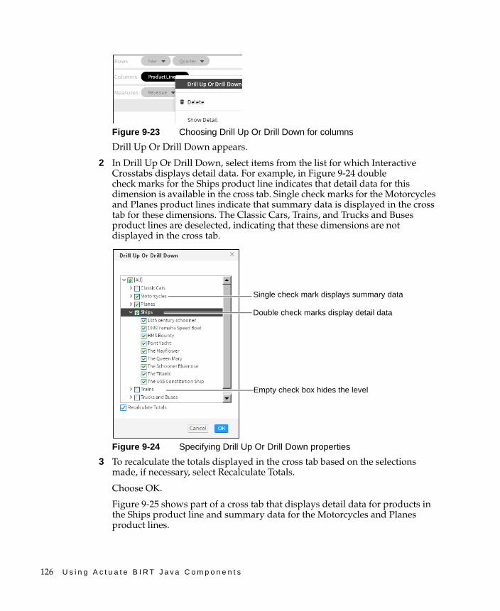
126 U s i n g A c t u a t e B I R T J a v a C o m p o n e n t s
Figure 9-23 Choosing Drill Up Or Drill Down for columns
Drill Up Or Drill Down appears.
2 In Drill Up Or Drill Down, select items from the list for which Interactive Crosstabs displays detail data. For example, in Figure 9-24 double check marks for the Ships product line indicates that detail data for this dimension is available in the cross tab. Single check marks for the Motorcycles and Planes product lines indicate that summary data is displayed in the cross tab for these dimensions. The Classic Cars, Trains, and Trucks and Buses product lines are deselected, indicating that these dimensions are not displayed in the cross tab.
Figure 9-24 Specifying Drill Up Or Drill Down properties
3 To recalculate the totals displayed in the cross tab based on the selections made, if necessary, select Recalculate Totals.
Choose OK.
Figure 9-25 shows part of a cross tab that displays detail data for products in the Ships product line and summary data for the Motorcycles and Planes product lines.
Double check marks display detail data
Single check mark displays summary data
Empty check box hides the level
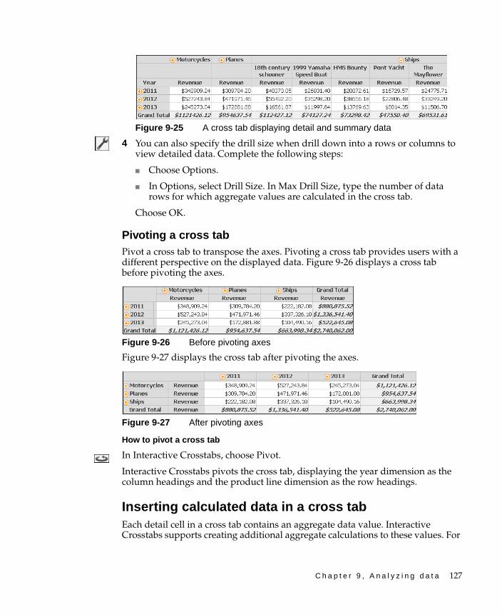
C h a p t e r 9 , A n a l y z i n g d a t a 127
Figure 9-25 A cross tab displaying detail and summary data
4 You can also specify the drill size when drill down into a rows or columns to view detailed data. Complete the following steps:
■ Choose Options.
■ In Options, select Drill Size. In Max Drill Size, type the number of data rows for which aggregate values are calculated in the cross tab.
Choose OK.
Pivoting a cross tabPivot a cross tab to transpose the axes. Pivoting a cross tab provides users with a different perspective on the displayed data. Figure 9-26 displays a cross tab before pivoting the axes.
Figure 9-26 Before pivoting axes
Figure 9-27 displays the cross tab after pivoting the axes.
Figure 9-27 After pivoting axes
How to pivot a cross tab
In Interactive Crosstabs, choose Pivot.
Interactive Crosstabs pivots the cross tab, displaying the year dimension as the column headings and the product line dimension as the row headings.
Inserting calculated data in a cross tabEach detail cell in a cross tab contains an aggregate data value. Interactive Crosstabs supports creating additional aggregate calculations to these values. For
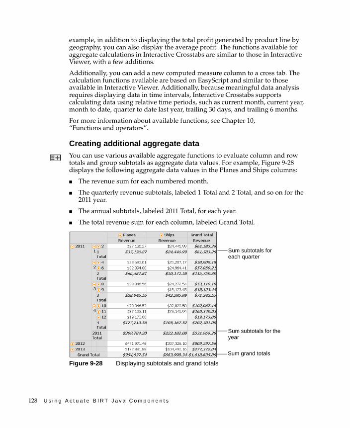
128 U s i n g A c t u a t e B I R T J a v a C o m p o n e n t s
example, in addition to displaying the total profit generated by product line by geography, you can also display the average profit. The functions available for aggregate calculations in Interactive Crosstabs are similar to those in Interactive Viewer, with a few additions.
Additionally, you can add a new computed measure column to a cross tab. The calculation functions available are based on EasyScript and similar to those available in Interactive Viewer. Additionally, because meaningful data analysis requires displaying data in time intervals, Interactive Crosstabs supports calculating data using relative time periods, such as current month, current year, month to date, quarter to date last year, trailing 30 days, and trailing 6 months.
For more information about available functions, see Chapter 10, “Functions and operators”.
Creating additional aggregate dataYou can use various available aggregate functions to evaluate column and row totals and group subtotals as aggregate data values. For example, Figure 9-28 displays the following aggregate data values in the Planes and Ships columns:
■ The revenue sum for each numbered month.
■ The quarterly revenue subtotals, labeled 1 Total and 2 Total, and so on for the 2011 year.
■ The annual subtotals, labeled 2011 Total, for each year.
■ The total revenue sum for each column, labeled Grand Total.
Figure 9-28 Displaying subtotals and grand totals
Sum grand totals
Sum subtotals for each quarter
Sum subtotals for the year

C h a p t e r 9 , A n a l y z i n g d a t a 129
You can display the grand totals and subtotals on columns and rows either before or after the detail values. You can use the Options dialog box to specify the location of grand totals and subtotals in the cross tab.
Adding a computed measureTo display computed data in a cross tab, you can create a column that displays calculated data based on an expression that Interactive Crosstabs evaluates. For a complete list of supported functions and their descriptions, see Chapter 10, “Functions and operators”.
Working with relative time periodsBecause analysis of stock performance, revenue, or productivity is typically meaningful only if it can be measured over time, such as by day, week, month, quarter, or year, Interactive Crosstabs supports several useful relative time period functions. For example, a cross tab can display revenue data for a particular month, quarter, or year. Figure 9-29 displays sales revenue by region by quarter for two years.
Figure 9-29 Displaying sales revenue by region by quarter for two years
Displaying data by relative time periods supports, for example, the comparison of current data with past data of the same period. Figure 9-30 shows profit year-to-date 2013 values, using the date 11/30/2013, and the comparable year-to-date values for the previous year for France, Japan, and the UK.
Figure 9-30 Displaying profit year-to-date in 2013 and previous year-to-date
How to create a calculation using a relative time period
1 In Interactive Crosstabs, choose New Computed Measure. Computed Measure appears.
2 In Computed Measure, shown in Figure 9-31, complete the following steps. The procedure can differ based on the selected category and time period.
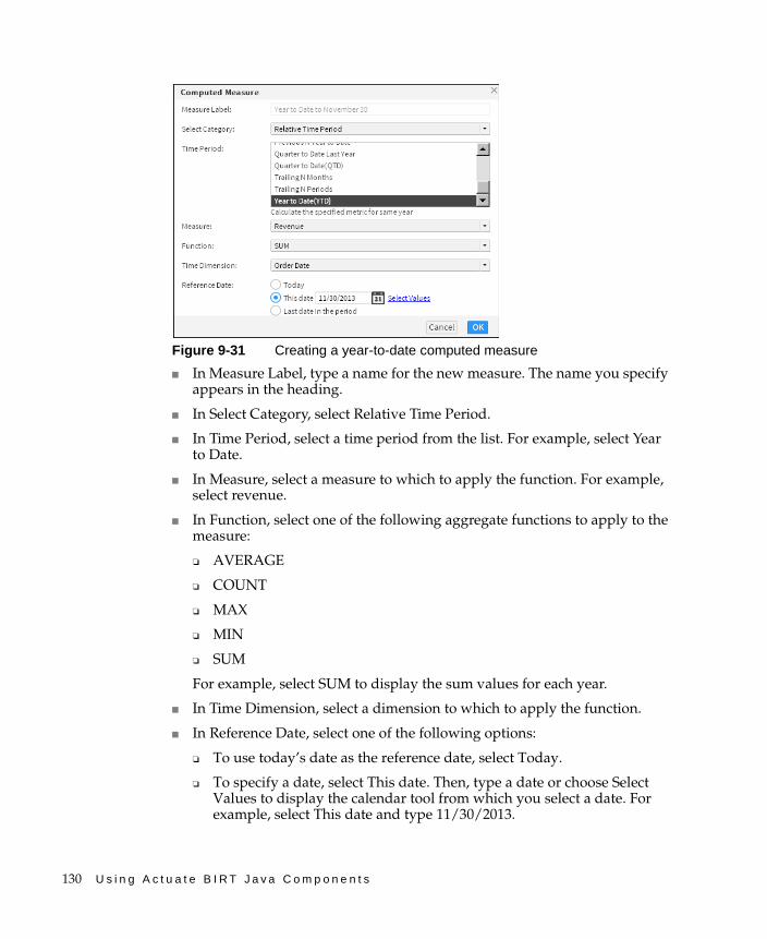
130 U s i n g A c t u a t e B I R T J a v a C o m p o n e n t s
Figure 9-31 Creating a year-to-date computed measure
■ In Measure Label, type a name for the new measure. The name you specify appears in the heading.
■ In Select Category, select Relative Time Period.
■ In Time Period, select a time period from the list. For example, select Year to Date.
■ In Measure, select a measure to which to apply the function. For example, select revenue.
■ In Function, select one of the following aggregate functions to apply to the measure:
❏ AVERAGE
❏ COUNT
❏ MAX
❏ MIN
❏ SUM
For example, select SUM to display the sum values for each year.
■ In Time Dimension, select a dimension to which to apply the function.
■ In Reference Date, select one of the following options:
❏ To use today’s date as the reference date, select Today.
❏ To specify a date, select This date. Then, type a date or choose Select Values to display the calendar tool from which you select a date. For example, select This date and type 11/30/2013.
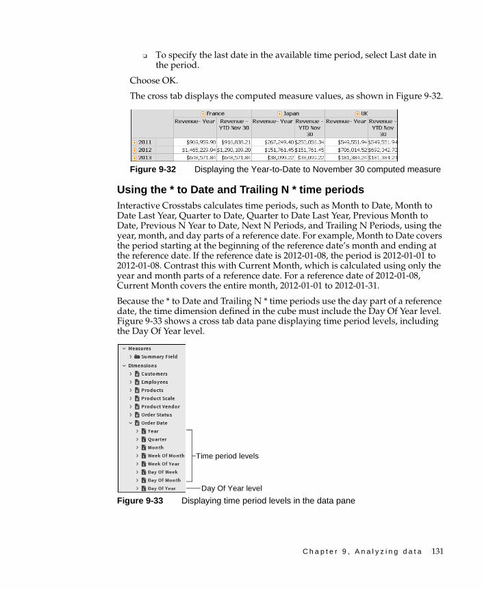
C h a p t e r 9 , A n a l y z i n g d a t a 131
❏ To specify the last date in the available time period, select Last date in the period.
Choose OK.
The cross tab displays the computed measure values, as shown in Figure 9-32.
Figure 9-32 Displaying the Year-to-Date to November 30 computed measure
Using the * to Date and Trailing N * time periodsInteractive Crosstabs calculates time periods, such as Month to Date, Month to Date Last Year, Quarter to Date, Quarter to Date Last Year, Previous Month to Date, Previous N Year to Date, Next N Periods, and Trailing N Periods, using the year, month, and day parts of a reference date. For example, Month to Date covers the period starting at the beginning of the reference date’s month and ending at the reference date. If the reference date is 2012-01-08, the period is 2012-01-01 to 2012-01-08. Contrast this with Current Month, which is calculated using only the year and month parts of a reference date. For a reference date of 2012-01-08, Current Month covers the entire month, 2012-01-01 to 2012-01-31.
Because the * to Date and Trailing N * time periods use the day part of a reference date, the time dimension defined in the cube must include the Day Of Year level. Figure 9-33 shows a cross tab data pane displaying time period levels, including the Day Of Year level.
Figure 9-33 Displaying time period levels in the data pane
Day Of Year level
Time period levels
132 U s i n g A c t u a t e B I R T J a v a C o m p o n e n t s
If the time dimension in the cube does not include the Day Of Year level, and you use a * to Date or a Next N * or Trailing N * time period in a relative time period calculation, the measures display the wrong results. Month to Date returns the same results as Current Month, Quarter to Date returns the same results as Current Quarter, and so on. In other words, the day part of the reference date has no effect.
Filtering data in a cross tabIn Interactive Crosstabs, you can create filter conditions at the cross tab level to narrow the scope of data displayed and make the cross tab easier to use. You can also create filters for dimensions and measures present in the cross tab’s cube or data model, but not in use in the cross tab.
Using filters can limit the ability to drill up or down to view summary or drill detail data in a cross tab. When you create a filter condition, take into consideration the data values you need to view and the trends or relationships that you aim to analyze. If you need to save a cube view (.cubeview) file or a BIRT document (.rptdocument) file, and share it with other users for analysis, consider how any filters you applied can limit the ability for others to drill up or drill down the data hierarchy.
When you apply a filter condition, select Recalculate Totals to enable Interactive Crosstabs to recalculate totals for the filtered data. If you want to retain existing totals for comparison with the filtered cross tab data, deselect Recalculate Totals. In this case, the cross tab displays columns and rows based on the filters you apply, but the original totals for the unfiltered data remain.
Creating a filter at the cross tab levelWhen you create a filter condition in Interactive Crosstabs, you specify the dimension, measure, row, or column, to evaluate, select a comparison operator, and specify a value to which to compare, as you did when creating a filter in Interactive Viewer. Defining a filter condition at the cross tab level displays only a subset of data retrieved from the cube or data model data source.
You can also create a slicer filter condition for dimension or measure data fields in the cube or data model data source that are not in use in the cross tab. Slicer filters limit the data retrieved from the cube or data model. This filter is specifically useful when working with cubes or data models containing large amounts of data.
For more information about comparison operators to use when you create filter condition expressions, see Chapter 10, “Functions and operators”.
How to create a filter at the cross tab level
You can use this procedure to create a filter condition using an attribute, dimension, or measure value from the cross tab.
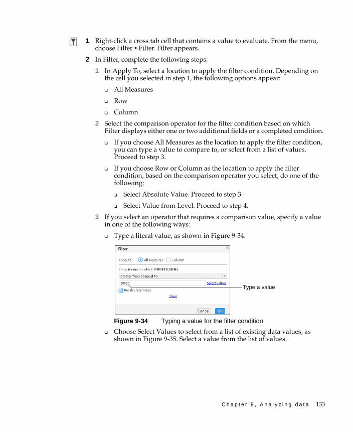
C h a p t e r 9 , A n a l y z i n g d a t a 133
1 Right-click a cross tab cell that contains a value to evaluate. From the menu, choose Filter➛Filter. Filter appears.
2 In Filter, complete the following steps:
1 In Apply To, select a location to apply the filter condition. Depending on the cell you selected in step 1, the following options appear:
❏ All Measures
❏ Row
❏ Column
2 Select the comparison operator for the filter condition based on which Filter displays either one or two additional fields or a completed condition.
❏ If you choose All Measures as the location to apply the filter condition, you can type a value to compare to, or select from a list of values. Proceed to step 3.
❏ If you choose Row or Column as the location to apply the filter condition, based on the comparison operator you select, do one of the following:
❏ Select Absolute Value. Proceed to step 3.
❏ Select Value from Level. Proceed to step 4.
3 If you select an operator that requires a comparison value, specify a value in one of the following ways:
❏ Type a literal value, as shown in Figure 9-34.
Figure 9-34 Typing a value for the filter condition
❏ Choose Select Values to select from a list of existing data values, as shown in Figure 9-35. Select a value from the list of values.
Type a value
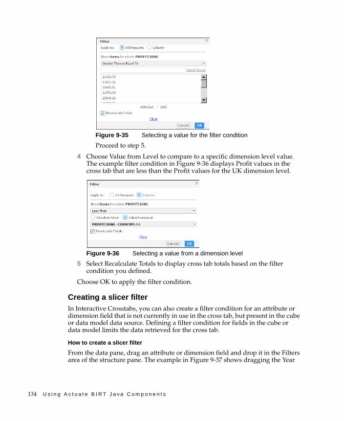
134 U s i n g A c t u a t e B I R T J a v a C o m p o n e n t s
Figure 9-35 Selecting a value for the filter condition
Proceed to step 5.
4 Choose Value from Level to compare to a specific dimension level value. The example filter condition in Figure 9-36 displays Profit values in the cross tab that are less than the Profit values for the UK dimension level.
Figure 9-36 Selecting a value from a dimension level
5 Select Recalculate Totals to display cross tab totals based on the filter condition you defined.
Choose OK to apply the filter condition.
Creating a slicer filterIn Interactive Crosstabs, you can also create a filter condition for an attribute or dimension field that is not currently in use in the cross tab, but present in the cube or data model data source. Defining a filter condition for fields in the cube or data model limits the data retrieved for the cross tab.
How to create a slicer filter
From the data pane, drag an attribute or dimension field and drop it in the Filters area of the structure pane. The example in Figure 9-37 shows dragging the Year
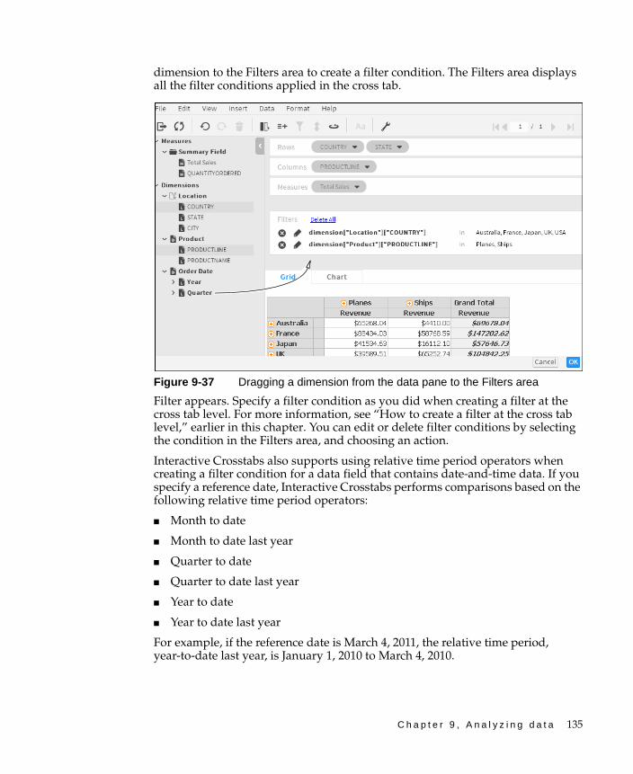
C h a p t e r 9 , A n a l y z i n g d a t a 135
dimension to the Filters area to create a filter condition. The Filters area displays all the filter conditions applied in the cross tab.
Figure 9-37 Dragging a dimension from the data pane to the Filters area
Filter appears. Specify a filter condition as you did when creating a filter at the cross tab level. For more information, see “How to create a filter at the cross tab level,” earlier in this chapter. You can edit or delete filter conditions by selecting the condition in the Filters area, and choosing an action.
Interactive Crosstabs also supports using relative time period operators when creating a filter condition for a data field that contains date-and-time data. If you specify a reference date, Interactive Crosstabs performs comparisons based on the following relative time period operators:
■ Month to date
■ Month to date last year
■ Quarter to date
■ Quarter to date last year
■ Year to date
■ Year to date last year
For example, if the reference date is March 4, 2011, the relative time period, year-to-date last year, is January 1, 2010 to March 4, 2010.
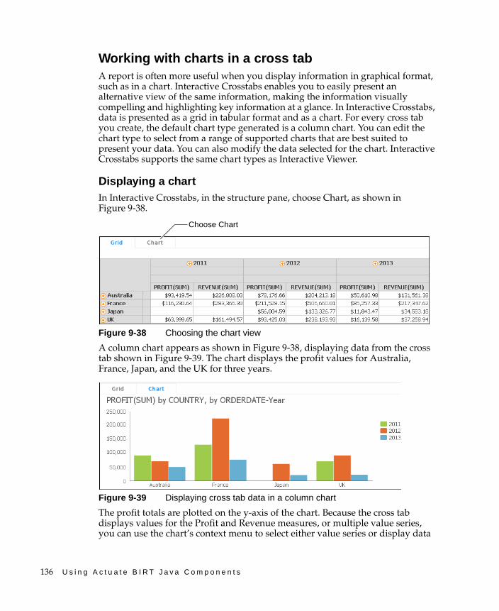
136 U s i n g A c t u a t e B I R T J a v a C o m p o n e n t s
Working with charts in a cross tabA report is often more useful when you display information in graphical format, such as in a chart. Interactive Crosstabs enables you to easily present an alternative view of the same information, making the information visually compelling and highlighting key information at a glance. In Interactive Crosstabs, data is presented as a grid in tabular format and as a chart. For every cross tab you create, the default chart type generated is a column chart. You can edit the chart type to select from a range of supported charts that are best suited to present your data. You can also modify the data selected for the chart. Interactive Crosstabs supports the same chart types as Interactive Viewer.
Displaying a chartIn Interactive Crosstabs, in the structure pane, choose Chart, as shown in Figure 9-38.
Figure 9-38 Choosing the chart view
A column chart appears as shown in Figure 9-38, displaying data from the cross tab shown in Figure 9-39. The chart displays the profit values for Australia, France, Japan, and the UK for three years.
Figure 9-39 Displaying cross tab data in a column chart
The profit totals are plotted on the y-axis of the chart. Because the cross tab displays values for the Profit and Revenue measures, or multiple value series, you can use the chart’s context menu to select either value series or display data
Choose Chart
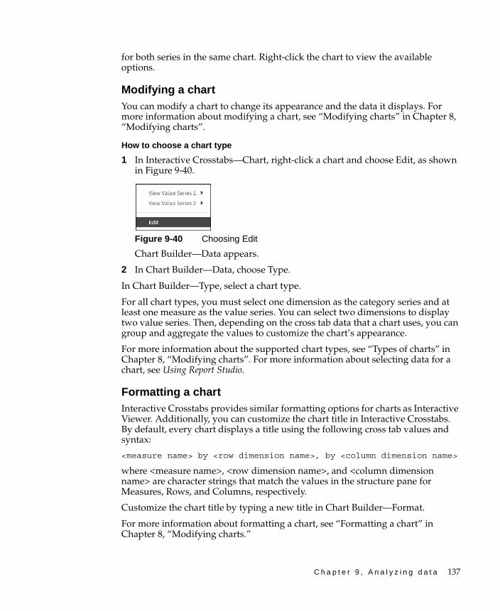
C h a p t e r 9 , A n a l y z i n g d a t a 137
for both series in the same chart. Right-click the chart to view the available options.
Modifying a chartYou can modify a chart to change its appearance and the data it displays. For more information about modifying a chart, see “Modifying charts” in Chapter 8, “Modifying charts”.
How to choose a chart type
1 In Interactive Crosstabs—Chart, right-click a chart and choose Edit, as shown in Figure 9-40.
Figure 9-40 Choosing Edit
Chart Builder—Data appears.
2 In Chart Builder—Data, choose Type.
In Chart Builder—Type, select a chart type.
For all chart types, you must select one dimension as the category series and at least one measure as the value series. You can select two dimensions to display two value series. Then, depending on the cross tab data that a chart uses, you can group and aggregate the values to customize the chart’s appearance.
For more information about the supported chart types, see “Types of charts” in Chapter 8, “Modifying charts”. For more information about selecting data for a chart, see Using Report Studio.
Formatting a chartInteractive Crosstabs provides similar formatting options for charts as Interactive Viewer. Additionally, you can customize the chart title in Interactive Crosstabs. By default, every chart displays a title using the following cross tab values and syntax:
<measure name> by <row dimension name>, by <column dimension name>
where <measure name>, <row dimension name>, and <column dimension name> are character strings that match the values in the structure pane for Measures, Rows, and Columns, respectively.
Customize the chart title by typing a new title in Chart Builder—Format.
For more information about formatting a chart, see “Formatting a chart” in Chapter 8, “Modifying charts.”

138 U s i n g A c t u a t e B I R T J a v a C o m p o n e n t s

C h a p t e r 1 0 , F u n c t i o n s a n d o p e r a t o r s 139
C h a p t e r
10Chapter 10Functions and operators
This chapter contains the following topics:
■ Functions
■ Functions used in computed column expressions
■ Functions used in aggregate calculations
■ Operators
140 U s i n g A c t u a t e B I R T J a v a C o m p o n e n t s
FunctionsThis section is a complete reference to all of the functions in Interactive Viewer, Interactive Crosstabs, and BIRT Studio. This reference organizes the functions into two sections based on those used in expressions when creating a computed column and functions that are used to perform aggregate calculations.
Functions used in computed column expressionsThe following list of functions appear when you create expressions to compute column data. Each function entry includes a general description of the function, its syntax, the arguments to the function, the result the function returns, and an example that shows typical usage. Use this reference to find information about a function that you want to use when you insert a computed column to display calculated data in a BIRT design.
% OFCalculates the percentage value of a selected measure compared to a selected base group value.
Category Math
Measure Select a measure name from the list.
% Base Select a base group from the list.
Returns For the selected measure, Interactive Crosstabs calculates the percentage of the base group total and displays the percentage value.
Example For example, compare a cross tab revenue value to the grand total of all revenue values, using the following calculation:
(<cross tab revenue value>/<cross tab revenue grand total>) * 100%
% OF COLUMNCalculates the percentage of the column total for each measure value in each column.
Category Math
Measure Select a measure name from the list.
C h a p t e r 1 0 , F u n c t i o n s a n d o p e r a t o r s 141
Returns For each measure in each column, Interactive Crosstabs calculates the percentage of the column total and displays the percentage value. The sum of percent-of-column values in each column is 100%.
Example In Measure, select the sales revenue measure. Interactive Crosstabs displays a percentage value in the cell next to each sales revenue value. The percentage value equals the sales revenue value divided by the column sum, and multiplied by 100%, as follows:
(<sales revenue value>/<column sum>) * 100%
% OF DIFFERENCECalculates the percentage of the difference between measure values.
Category Math
Measure Select the first measure name from the list.
Measure Select the second measure name from the list.
Returns Interactive Crosstabs calculates the percentage of the difference between the second measure and the first measure, as follows:
((measureB - measureA)/measureA) * 100%
Interactive Crosstabs displays the percentage of the difference in the cross tab cells.
% OF ROWCalculates the percentage of the row total for each measure in each row.
Category Math
Measure Select a measure name from the list.
Returns For each measure in each row, Interactive Crosstabs calculates the percentage of the row total and displays the percentage value, as follows:
(<measure value>/<row sum>) * 100%
The sum of percent-of-row values in each row is 100%.
Example In Measure, select the sales revenue measure. Interactive Crosstabs displays a percentage value in the cell next to each sales revenue value. The percentage value equals the sales revenue value divided by the row total, and multiplied by 100%.
142 U s i n g A c t u a t e B I R T J a v a C o m p o n e n t s
% OF TOTALCalculates the percentage of the cross tab grand total for each measure in each column and row.
Category Math
Measure Select a measure name from the list.
Returns For each measure in each column and row, Interactive Crosstabs calculates the percentage of the cross tab grand total and displays the percent value, as follows
(<measure value>/<cross tab grand total>) * 100%
The sum of all percent-of-total values in the cross tab is 100%.
Example In Measure, select the sales revenue measure. Interactive Crosstabs displays a percentage value in the cell next to each sales revenue value. The percentage value equals the sales revenue value, divided by the row total, and multiplied by 100%.
ABS( )Returns the absolute value of a number without regard to its sign. For example, 6 is the absolute value of 6 and -6.
Syntax ABS(num)
Argument numThe number, or numeric expression that specifies the number, for which you want to find the absolute value.
Returns A number that represents the absolute value of num.
Example The following example returns the absolute value for each number in the TemperatureCelsius data field:
ABS([TemperatureCelsius])
ADD_DAY( )Adds a specified number of days to a date value.
Syntax ADD_DAY(date, daysToAdd)
Arguments dateThe date or date expression that represents the start date.
C h a p t e r 1 0 , F u n c t i o n s a n d o p e r a t o r s 143
daysToAddThe number of days to add to the start date. If you specify a negative number, the result appears to subtract the number from the start date.
Returns The date value that results from adding the specified number of days to the start date.
Example The following example adds 15 days to each date value in the InvoiceDate data field:
ADD_DAY([InvoiceDate], 15)
ADD_HOUR( )Adds a specified number of hours to a date value.
Syntax ADD_HOUR(date, hoursToAdd)
Arguments dateThe date or date expression that represents the start date. If a start date does not have a time value, the function assumes the time is midnight, 12:00 AM.
hoursToAddThe number of hours to add to the start date. If you specify a negative number, the result appears to subtract the number from the start date.
Returns The date-and-time value that results from adding the specified number of hours to the start date.
Example The following example adds eight hours to each date value in the ShipDate data field:
ADD_HOUR([ShipDate], 8)
ADD_MINUTE( )Adds a specified number of minutes to a date value.
Syntax ADD_MINUTE(date, minutesToAdd)
Arguments dateThe date or date expression that represents the start date. If a start date does not have a time value, the function assumes the time is midnight, 12:00 AM.
minutesToAddThe number of minutes to add to the start date. If you specify a negative number, the result appears to subtract the number from the start date.
Returns The date-and-time value that results from adding the specified number of minutes to the start date.
144 U s i n g A c t u a t e B I R T J a v a C o m p o n e n t s
Example The following example subtracts 30 minutes from each date in the StartTime data field:
ADD_MINUTE([StartTime], -30)
ADD_MONTH( )Adds a specified number of months to a date value.
Syntax ADD_MONTH(date, monthsToAdd)
Arguments dateThe date or date expression that represents the start date.
monthsToAddThe number of months to add to the start date. If you specify a negative number, the result appears to subtract the number from the start date.
Returns The date value that results from adding the specified number of months to the start date. This function always returns a valid date. If necessary, the day part of the resulting date is adjusted downward to the last day of the resulting month in the resulting year. For example, if you add one month to 1/31/08, ADD_MONTH( ) returns 2/29/08, not 2/31/08 or 2/28/08, because 2008 is a leap year.
Example The following example adds two months to each date value in the InitialRelease data field:
ADD_MONTH([InitialRelease], 2)
ADD_QUARTER( )Adds a specified number of quarters to a date value.
Syntax ADD_QUARTER(date, quartersToAdd)
Arguments dateThe date or date expression that represents the start date.
quartersToAddThe number of quarters to add to the start date. If you specify a negative number, the result appears to subtract the number from the start date.
Returns The date value that results from adding the specified number of quarters to the start date. A quarter is equal to three months. For example, if you add two quarters to 9/22/08, ADD_QUARTER( ) returns 3/22/09.
C h a p t e r 1 0 , F u n c t i o n s a n d o p e r a t o r s 145
Example The following example adds two quarters to each date value in the ForecastClosing data field:
ADD_QUARTER([ForecastClosing], 2)
ADD_SECOND( )Adds a specified number of seconds to a date value.
Syntax ADD_SECOND(date, secondsToAdd)
Arguments dateThe date or date expression that represents the start date. If a start date does not have a time value, the function assumes the time is midnight, 12:00 AM.
secondsToAddThe number of seconds to add to the start date. If you specify a negative number, the result appears to subtract the number from the start date.
Returns The date-and-time value that results from adding the specified number of seconds to the start date.
Example The following example adds 30 seconds to each date value in the StartTime data field:
ADD_SECOND([StartTime], 30)
ADD_WEEK( )Adds a specified number of weeks to a date value.
Syntax ADD_WEEK(date, weeksToAdd)
Arguments dateThe date or date expression that represents the start date.
weeksToAddThe number of weeks to add to the start date. If you specify a negative number, the result appears to subtract the number from the start date.
Returns The date value that results from adding the number of weeks to the start date.
Example The following example adds two weeks to each date value in the OrderDate data field:
ADD_WEEK([OrderDate], 2)
146 U s i n g A c t u a t e B I R T J a v a C o m p o n e n t s
ADD_YEAR( )Adds a specified number of years to a date value.
Syntax ADD_YEAR(date, yearsToAdd)
Arguments dateThe date or date expression that represents the start date.
yearsToAddThe number of years to add to the start date. If you specify a negative number, the result appears to subtract the number from the start date.
Returns The date value that results from adding the number of years to the start date.
Example The following example adds five years to each date value in the HireDate data field:
ADD_YEAR([HireDate], 5)
BETWEEN( )Tests if a value is between two specified values.
Syntax BETWEEN(value, upperBound, lowerBound)
Arguments valueThe value to test. The value can be a string, numeric, or date value.
upperBoundThe first value in the range of values to which to compare. String and date values must be enclosed in double quotation marks (" ").
lowerBoundThe second value in the range of values to which to compare. String and date values must be enclosed in double quotation marks (" ").
Returns True if value is between upperBound and lowerBound, or equal to upperBound or lowerBound; returns false otherwise.
Examples The following example tests each value in the SalesTotal data field to see if the value is between 10000 and 20000:
BETWEEN([SalesTotal], 10000, 20000)
The following example tests each value in the CustomerName data field to see if the value is between A and M:
BETWEEN([CustomerName], "A", "M")
C h a p t e r 1 0 , F u n c t i o n s a n d o p e r a t o r s 147
The following example tests each value in the ReceiptDate data field to see if the value is between 10/01/07 and 12/31/07:
BETWEEN([ReceiptDate], "10/01/07 12:00 AM", "12/31/07 12:00 AM")
The following example uses BETWEEN( ) in conjunction with the IF( ) and ADD_DAY( ) functions to calculate a shipment date. If an orderDate value is in December 2007 (between 12/1/07 and 12/31/07), add five days to the orderDate value. If an orderDate value is in a month other than December, add three days to the orderDate value.
IF((BETWEEN([orderDate], "12/1/07 12:00 AM", "12/31/07 12:00 AM")), (ADD_DAY([orderDate], 5)), (ADD_DAY([orderDate], 3)))
CEILING( )Rounds a number up to the nearest specified multiple.
Syntax CEILING(num, significance)
Arguments numThe numeric value to round up.
significanceThe multiple up to which to round num.
Returns The number that results from the rounding. If num is an exact multiple of significance, no rounding occurs.
Examples CEILING( ) is commonly used to round up prices. For example, to avoid dealing with pennies, if the Price value is 20.52, CEILING( ) returns 20.55. You can round prices in a Price data field up to the nearest nickel with the following expression:
CEILING([Price], 0.05)
If the Price value is 20.52, CEILING( ) returns 20.60. If the Price value is 20.40, CEILING( ) returns 20.40. No rounding occurs because 20.40 is already a multiple of 0.1. The following example rounds prices up to the nearest dime:
CEILING([Price], 0.1)
The following example rounds prices up to the nearest dollar. If the Price value is 20.30, CEILING( ) returns 21.0.
CEILING([Price], 1)
DAY( )Returns a number from 1 to 31 that represents the day of the month.
148 U s i n g A c t u a t e B I R T J a v a C o m p o n e n t s
Syntax DAY(date)
Argument dateThe date or date expression from which you want to extract the day.
Returns The number of the day of the month for the specified date value.
Example The following example gets the number of the day for each date value in the ShipDate data field:
DAY([ShipDate])
DIFF_DAY( )Calculates the number of days between two date values.
Syntax DIFF_DAY(date1, date2)
Arguments date1The first date or date expression to use in the calculation.
date2The second date or date expression to use in the calculation.
Returns The number of days between date1 and date2.
Example The following example calculates the number of days between each value in the invoiceDate data field and each value in the paymentDate data field:
DIFF_DAY([invoiceDate],[paymentDate])
The results show how long it takes to pay invoices.
The following example calculates the number of days from an order date to Christmas:
DIFF_DAY([orderDate], "12/25/08")
The following example calculates the number of days from the current date to Christmas. TODAY( ) is a function that returns the current date:
DIFF_DAY(TODAY(), "12/25/08")
DIFF_HOUR( )Calculates the number of hours between two date values.
Syntax DIFF_HOUR(date1, date2)
Arguments date1The first date or date expression to use in the calculation. If the date does not have a time value, the function assumes the time is midnight, 12:00 AM.
C h a p t e r 1 0 , F u n c t i o n s a n d o p e r a t o r s 149
date2The second date or date expression to use in the calculation. If the date does not have a time value, the function assumes the time is midnight, 12:00 AM.
Returns The number of hours between date1 and date2.
Example The following example calculates the number of hours between each value in the startTime data field and each value in the finishTime data field:
DIFF_HOUR([startTime],[finishTime])
The following example calculates the number of hours from the current date to Christmas. NOW( ) is a function that returns the current date and time. If you supply a literal date as an argument, you must include the time value, as shown in the following example:
DIFF_HOUR(NOW(), "12/25/08 12:00 AM")
DIFF_MINUTE( )Calculates the number of minutes between two date values.
Syntax DIFF_MINUTE(date1, date2)
Arguments date1The first date or date expression to use in the calculation. If the date does not have a time value, the function assumes the time is midnight, 12:00 AM.
date2The second date or date expression to use in the calculation. If the date does not have a time value, the function assumes the time is midnight, 12:00 AM.
Returns The number of minutes between date1 and date2.
Example The following example calculates the number of minutes between each value in the startTime data field and each value in the finishTime data field:
DIFF_MINUTE([startTime],[finishTime])
The following example calculates the number of minutes from the current date to Christmas. NOW( ) is a function that returns the current date and time. If you supply a literal date as an argument, you must include the time value, as shown in the following example:
DIFF_MINUTE(NOW(), "12/25/08 12:00 AM")
DIFF_MONTH( )Calculates the number of months between two date values.
150 U s i n g A c t u a t e B I R T J a v a C o m p o n e n t s
Syntax DIFF_MONTH(date1,date2)
Arguments date1The first date or date expression to use in the calculation.
date2The second date or date expression to use in the calculation.
Returns The number of months between date1 and date2. The function calculates the difference by subtracting the month number of date1 from the month number of date2. For example, if date1 is 8/1/08 and date2 is 8/31/08, DIFF_MONTH( ) returns 0. If date1 is 8/25/08 and date2 is 9/5/08, DIFF_MONTH( ) returns 1.
Example The following example calculates the number of months between each value in the askByDate data field and each value in the ShipByDate data field:
DIFF_MONTH([askByDate],[shipByDate])
The following example calculates the number of months from each value in the hireDate data field to the end of the year:
DIFF_MONTH([hireDate], "1/1/09")
DIFF_QUARTER( )Calculates the number of quarters between two date values.
Syntax DIFF_QUARTER(date1, date2)
Arguments date1The first date or date expression to use in the calculation.
date2The second date or date expression to use in the calculation.
Returns The number of quarters between date1 and date2. DIFF_QUARTER calculates the difference by subtracting the month number of date1 from the month number of date2. A difference of three months is equal to one quarter. For example, if date1 is 8/1/08 and date2 is 10/31/08, DIFF_QUARTER( ) returns 0. If date1 is 8/25/08 and date2 is 11/5/08, DIFF_QUARTER( ) returns 1.
Example The following example calculates the number of quarters between each value in the PlanClosing data field and each value in the ActualClosing data field:
DIFF_QUARTER([PlanClosing],[ActualClosing])
The following example calculates the number of quarters from each value in the orderDate data field to the end of the year:
DIFF_QUARTER([orderDate], "1/1/09")
C h a p t e r 1 0 , F u n c t i o n s a n d o p e r a t o r s 151
DIFF_SECOND( )Calculates the number of seconds between two date values.
Syntax DIFF_SECOND(date1, date2)
Arguments date1The first date or date expression to use in the calculation. If the date does not have a time value, the function assumes the time is midnight, 12:00 AM.
date2The second date or date expression to use in the calculation. If the date does not have a time value, the function assumes the time is midnight, 12:00 AM.
Returns The number of seconds between date1 and date2.
Example The following example calculates the number of seconds between each value in the startTime data field and each value in the finishTime data field:
DIFF_SECOND([startTime],[finishTime])
The following example calculates the number of seconds from the current date to Christmas. NOW( ) is a function that returns the current date and time. If you supply a literal date as an argument, you must include the time value, as shown in the following example:
DIFF_SECOND(NOW(), "12/24/08 12:00 AM")
DIFF_WEEK( )Calculates the number of weeks between two date values.
Syntax DIFF_WEEK(date1, date2)
Arguments date1The first date or date expression to use in the calculation.
date2The second date or date expression to use in the calculation.
Returns The number of weeks between date1 and date2. The function calculates the difference by subtracting the week number of date1 from the week number of date2. For example, if date1 is 1/3/08 (week 1 of the year), and date2 is 1/7/08 (week 2 of the year), DIFF_WEEK( ) returns 1.
Example The following example calculates the number of weeks between each value in the askByDate data field and each value in the shipByDate data field:
DIFF_WEEK([askByDate],[shipByDate])
152 U s i n g A c t u a t e B I R T J a v a C o m p o n e n t s
The following example calculates the number of weeks from each value in the orderDate data field to the end of the year:
DIFF_WEEK([orderDate], "1/1/09")
DIFF_YEAR( )Calculates the number of years between two date values.
Syntax DIFF_YEAR(date1, date2)
Arguments date1The first date or date expression to use in the calculation.
date2The second date or date expression to use in the calculation.
Returns The number of years between date1 and date2. The function calculates the difference by subtracting the year number of date1 from the year number of date2. For example, if date1 is 1/1/08 and date2 is 12/31/08, DIFF_YEAR( ) returns 0. If date1 is 11/25/08 and date2 is 1/5/09, DIFF_YEAR( ) returns 1.
Example The following example calculates the number of years between each value in the HireDate data field and each value in the TerminationDate data field:
DIFF_YEAR([HireDate],[TerminationDate])
The following example calculates the number of years from each value in the HireDate data field to the current date. TODAY( ) is a function that returns the current date:
DIFF_YEAR([HireDate], TODAY())
FIND( )Finds the location of a substring in a string.
Syntax FIND(strToFind, str)
FIND(strToFind, str, startPosition)
Arguments strToFindThe substring to search for. The search is case-sensitive.
strThe string in which to search.
startPositionThe position in str where the search starts.
C h a p t e r 1 0 , F u n c t i o n s a n d o p e r a t o r s 153
Returns The numerical position of the substring in the string. The first character of a string starts at 1. If the substring is not found, FIND( ) returns 0.
Example The following example searches for the substring, Ford, in each ProductName value:
FIND("Ford", [ProductName])
If the product name is 1969 Ford Falcon, FIND( ) returns 6.
The following example searches for the first hyphen (-) in each product code:
FIND("-", [ProductCode])
If the product code is ModelA-1234-567, FIND( ) returns 7.
The following example uses FIND( ) in conjunction with the LEFT( ) function to display the characters that precede the hyphen in a product code. The LEFT( ) function extracts a substring of a specified length, starting from the first character. In this example, the length of the substring to display is equal to the numerical position of the hyphen character.
LEFT([ProductCode], FIND("-", [ProductCode]))
If the product code is ModelA-1234, LEFT( ) returns the following string:
ModelA
IF( )Returns one value if a specified condition evaluates to TRUE, or another value if the condition evaluates to FALSE.
Syntax IF(condition, doIfTrue, doIfFalse)
Arguments conditionThe condition to test.
doIfTrueThe value to return if condition evaluates to TRUE.
doIfFalseThe value to return if condition evaluates to FALSE.
Returns Returns the doIfTrue value if condition is TRUE or the doIfFalse value if condition is FALSE.
Example The following example calculates and displays different discount amounts based on the value in the Total data field. If the Total value is greater than 5000, the discount is 15%. Otherwise, the discount is 10%.
IF([Total]>5000, [Total]*15%, [Total]*10%)
154 U s i n g A c t u a t e B I R T J a v a C o m p o n e n t s
The following example uses IF( ) in conjunction with the BETWEEN( ) and ADD_DAY( ) functions to calculate a shipment date. If an orderDate value is in December 2007 (between 12/1/07 and 12/31/07), add five days to the orderDate value. If a orderDate value is in a month other than December, add three days to the orderDate value.
IF((BETWEEN([orderDate], "12/1/07 12:00 AM", "12/31/07 12:00 AM")), (ADD_DAY([orderDate], 5)), (ADD_DAY([orderDate], 3)))
The following example checks each value in the Office data field. If the value is Boston, San Francisco, or NYC, the computed column displays U.S. If the value is something other than Boston, San Francisco, or NYC, the computed column displays Europe and Asia Pacific.
IF([Office]="Boston" OR [Office]="San Francisco" OR [Office]="NYC", "U.S.", "Europe and Asia Pacific")
IN( )Tests if a value is equal to a value in a list.
Syntax IN(value, check1,..., checkN)
Arguments valueThe value to test. The value can be a string, numeric, or date value.
check1, ..., checkNThe value or values to which to compare.
Returns True if value is equal to one of the check values; returns false otherwise.
Example The following example tests if New Haven, Baltimore, or Cooperstown are values in the city data field. If any one of the cities is in the data field, IN( ) returns true.
IN([city], "New Haven", "Baltimore", "Cooperstown")
The following example tests if 9/15/08 or 9/30/08 are values in the payDate data field. If you supply a literal date as an argument, you must include the time value, as shown in the following example:
IN([payDate], "9/15/08 12:00 AM", "9/30/08 12:00 AM")
The following example uses IN( ) in conjunction with the IF( ) function to test if Ships or Trains are values in the ProductLine data field. If Ships or Trains is a value in the field, the computed column displays Discontinued Item; otherwise, the product line value is displayed as it appears in the field.
IF(IN([ProductLine], "Ships", "Trains"),"Discontinued Item", [ProductLine])
C h a p t e r 1 0 , F u n c t i o n s a n d o p e r a t o r s 155
ISNULL( )Tests if a value in a specified data field is a null value. A null value means that no value exists.
Syntax ISNULL(value)
Argument valueThe data field in which to check for null values.
Returns True if a value in the specified data field is a null value; returns false otherwise.
Example The following example uses ISNULL( ) in conjunction with the IF( ) function to test for null values in the BirthDate data field. If there is a null value, the computed column displays No date specified; otherwise the BirthDate value is displayed.
IF(ISNULL([BirthDate]), "No date specified", [BirthDate])
LEFT( )Extracts a substring from a string, starting from the leftmost, or first, character.
Syntax LEFT(str)
LEFT(str, n)
Arguments strThe string from which to extract a substring.
nThe number of characters to extract, starting from the first character.
Returns A substring of a specific length:
■ If you omit n, the number of characters to extract, the function returns the first character only.
■ If n is zero, the function returns an empty string.
■ If n is greater than the length of the string, the function returns the entire string.
Example The following example displays the first letter of each name in the CustomerName data field:
LEFT([CustomerName])
The following example uses the LEFT( ) and FIND( ) functions to display the characters that precede the hyphen in a product code:
LEFT([ProductCode], FIND("-", [ProductCode]))

156 U s i n g A c t u a t e B I R T J a v a C o m p o n e n t s
If the product code is ModelA-1234, LEFT( ) returns the following string:
ModelA
LEN( )Counts the number of characters in a string.
Syntax LEN(str)
Argument strThe string expression to evaluate.
Returns The number of characters in the specified string.
Example The following example returns the length of each value in the ProductCode data field:
LEN([ProductCode])
The following example uses LEN( ) in conjunction with the RIGHT( ) and FIND( ) functions to display the characters that appear after the hyphen in a product code. RIGHT( ) extracts a substring of a specified length, starting from the last character. In this example, the length of the entire string returned by LEN( ) minus the length up to the hyphen is the number of characters to display.
RIGHT( [PRODUCTNAME], LEN([PRODUCTNAME] ) - (FIND("-" ,[PRODUCTNAME] )))
If the product code is ModelA-Ford, RIGHT( ) returns the following string:
A-Ford
LIKE( )Tests if a string matches a pattern.
Syntax LIKE(str, pattern)
strThe string to evaluate.
patternThe string pattern to match. You must enclose the pattern in double quotation marks (" "). The match is case-sensitive. You can use the following special characters in a pattern:
■ A percent character (%) matches zero or more characters. For example, %ace% matches any string value that contains the substring ace, such as Facebook,
C h a p t e r 1 0 , F u n c t i o n s a n d o p e r a t o r s 157
and MySpace. It does not match Ace Corporation because this string contains a capital A, and not the lowercase a.
■ An underscore character (_) matches exactly one character. For example, t_n matches tan, ten, tin, and ton. It does not match teen or tn.
To match a literal percent (%), underscore (_), precede those characters with two backslash (\\) characters. For example, to see if a string contains M_10, specify the following pattern:
"%M\\_10%"
Returns True if the string matches the pattern; returns false otherwise.
Example The following example returns true for values in the customerName field that start with D:
LIKE([customerName], "D%")
The following example returns true for productCode values that contain the substring Ford:
LIKE([productCode], "%Ford%")
The following example uses two LIKE( ) expressions to look for the substrings "Ford" or "Chevy" in each ProductName value. If a product name contains either substring, the computed column displays U.S. Model; otherwise, it displays Imported Model.
IF(((LIKE([ProductName], "%Ford%") = TRUE) OR (LIKE([ProductName], "%Chevy%") = TRUE)), "U.S. model", "Imported Model")
LOWER( )Converts all letters in a string to lowercase.
Syntax LOWER(str)
Argument strThe string to convert to lowercase.
Returns The specified string in all lowercase letters.
Example The following example displays all the string values in the productLine data field in lowercase:
LOWER([productLine])
MATCH( )Returns a Boolean indicating whether a pattern exists within a string.
158 U s i n g A c t u a t e B I R T J a v a C o m p o n e n t s
Syntax MATCH(source, pattern)
Arguments sourceThe string to evaluate.
patternThe string pattern to match. The pattern uses ECMAScript (JavaScript) syntax, as defined in Section 15.10 of Standard ECMA-262.
Returns True if the pattern matches, false otherwise.
Example The following example uses ECMAScript syntax in the pattern to detect any set of characters followed by the letter C, and returns true:
MATCH("ABC",".*C")
The following example checks whether the string starts with the letter X, followed by any single character, and ending with C. It returns false:
MATCH("ABC","X.C")
MOD( )Returns the modulo value for a number and a divisor.
Syntax MOD(number, divisor)
Arguments numberThe number from which to derive the mod value.
divisorThe divisor for the mod function.
Returns Returns the remainder value of number divided by divisor.
Example The following example computes the remainder of PriceEstimate data field divided by 12, returning an integer. For example, if the PriceEstimate value is 27365, MOD( ) returns 5.
MOD([PriceEstimate], 12)
MONTH( )Returns the month for a specified date value.
Syntax MONTH(date)
MONTH(date, option)
Arguments dateThe date or date expression whose month to get.
C h a p t e r 1 0 , F u n c t i o n s a n d o p e r a t o r s 159
optionA number that represents the month format to return. Use one of the following values:
■ 1 to get the month as a number from 1 to 12.
■ 2 to get the full month name, for example, January. The result is locale-specific.
■ 3 to get the abbreviated month name, for example, Jan. The result is locale-specific.
If you omit option, MONTH( ) returns the month as a number.
Returns The month for a specified date value.
Example The following example returns the month (1 – 12) for each value in the ShipDate data field:
MONTH([ShipDate])
The following example returns the full month name for each ShipDate value:
MONTH([ShipDate], 2)
NOT( )Negates a Boolean expression.
Syntax NOT(expression)
Argument expressionThe Boolean value or expression to negate.
Returns True if the expression evaluates to FALSE, and false if the expression evaluates to TRUE.
Example The following example uses NOT( ) in conjunction with the IF( ) and LIKE( ) functions. It tests if the value in the State data field is not CA. If the value is not CA, it returns the value of the Markup data field multiplied by 10%. If the value is CA it returns the value of the Markup data field multiplied by 15%:
IF(NOT(LIKE([State], "CA")),[Markup]*10%,[Markup]*15%)
The previous IF( ) statement is semantically equivalent to the following statement:
IF(LIKE([State], "CA"),[Markup]*15%,[Markup]*10%)
NOTNULL( )Tests if a value in a specified data field is a non-null value.
160 U s i n g A c t u a t e B I R T J a v a C o m p o n e n t s
Syntax NOTNULL(value)
Argument valueThe data field in which to check for non-null values.
Returns True if a value in the specified data field is not a null value; returns false otherwise.
Example The following example uses NOTNULL( ) in conjunction with the IF( ) function to test for non-null values in the BirthDate data field. If there is a non-null value, the BirthDate value is displayed; otherwise the string "No date specified" is displayed.
IF(NOTNULL([BirthDate]), [BirthDate], "No date specified")
NOW( )Returns the current date and time.
Syntax NOW( )
Returns The current date and time. For example:
Sep 23, 2008 11:56 AM
Example The following example uses the DIFF_MINUTE( ) and NOW( ) functions to calculate the number of minutes from the current date and time to Christmas:
DIFF_MINUTE(NOW(), "12/25/08 12:00 AM")
QUARTER( )Returns the quarter number for a specified date value.
Syntax QUARTER(date)
Arguments dateThe date or date expression whose quarter number to get.
Returns A number from 1 to 4 that represents the quarter for a specified date value. Quarter 1 starts in January.
Example The following example displays the quarter number for each value in the CloseDate data field:
QUARTER([CloseDate])
The following example displays a string—Q1, Q2, Q3, or Q4—for each value in the CloseDate data field:
"Q" & QUARTER([CloseDate])
C h a p t e r 1 0 , F u n c t i o n s a n d o p e r a t o r s 161
RANK( )Returns the rank of a value in a set of values. The rank of a value ranges from 1 to the number of values in the set. If two values are identical, they have the same rank.
Syntax RANK(expr)
RANK(expr, ascending, groupLevel)
Arguments exprThe expression that specifies the values to evaluate. The field can be of string, numeric, or date type.
ascendingUse one of the following values:
■ 0 to rank values in descending order. In descending order, the highest value is ranked 1, and the lowest value is equal to the number of values in the set.
■ 1 to rank values in ascending order. In ascending order, the lowest value is ranked 1, and the highest value is equal to the number of values in the set.
If you omit the ascending argument, RANK( ) assumes 0 (descending order).
groupLevelThe numeric index of the group whose values to use in the calculation. 0 indicates the table, 1 indicates the first group, 2 indicates the second group, and so on. If you do not supply a value for groupLevel, the function performs the calculation over all the values in the table.
Returns A number that represents the rank of a value in the specified data field in the table or in the specified group.
Example The following example ranks each value in the Score data field. The ranking is performed over all the values in the table.
RANK([Score])
The following example ranks each value in the Score data field in ascending order. The ranking is performed over all the values in each group at the second level.
RANK([Score], 1, 2)
RATIOReturns the ratio, MeasureA/MeasureB.
Category Math

162 U s i n g A c t u a t e B I R T J a v a C o m p o n e n t s
Measure Select the first measure name from the list.
Measure Select the second measure name from the list.
Returns Interactive Crosstabs divides the first measure value by the second measure value and displays the ratio value.
Example In a product line column, display a revenue column and a customer count column. Use the computed measure, Ratio, to divide revenue by the number of customers. Display the ratio in a Ratio of Revenue to CustomerCount column, as shown in Figure 10-1. Where the results of division by zero or an empty value occurs, NaN indicates the ratio value is not a number.
Figure 10-1 Displaying computed ratio values
RIGHT( )Extracts a substring from a string, starting from the rightmost, or last, character.
Syntax RIGHT(str)
RIGHT(str, n)
Arguments strThe string from which to extract a substring.
nThe number of characters to extract, starting from the last character.
Returns A substring of a specific length.
■ If you omit n, the number of characters to extract, the function returns the last character only.
■ If n is zero, the function returns an empty string.
■ If n is greater than the length of the string, the function returns the entire string.
C h a p t e r 1 0 , F u n c t i o n s a n d o p e r a t o r s 163
Example The following example displays the last four characters of each value in the ProductCode data field:
RIGHT([ProductCode], 4)
The following example uses RIGHT( ) in conjunction with the LEN( ) and FIND( ) functions to display the characters that appear after the hyphen in a product code. This example assumes that the number of characters after the hyphen varies. Therefore, the length of the entire string (returned by LEN( )) minus the length up to the hyphen (returned by FIND( )) is the number of characters to display.
RIGHT([ProductCode], (LEN([ProductCode]) - FIND("-" , [ProductCode])))
If the product code is ModelA-Ford, RIGHT( ) returns Ford. If the product code is ModelB-Toyota, RIGHT( ) returns Toyota.
ROUND( )Rounds a number to a specified number of digits.
Syntax ROUND(num)
ROUND(num, dec)
Arguments numThe number to round.
decThe number of digits up to which to round num. If you omit dec, ROUND( ) assumes 0.
Returns A number rounded to a specified number of digits.
Example The following example rounds the numbers in the PriceEstimate data field to return an integer. For example, if the PriceEstimate value is 1545.50, ROUND( ) returns 1546. If the PriceEstimate value is 1545.25, ROUND( ) returns 1545.
ROUND([PriceEstimate])
The following example rounds the numbers in the PriceEstimate data field to one decimal place. For example, if the PriceEstimate value is 1545.56, ROUND( ) returns 1545.6. If the PriceEstimate value is 1545.23, ROUND( ) returns 1545.2.
ROUND([PriceEstimate], 1)
The following example rounds the numbers in the PriceEstimate data field to one digit to the left of the decimal point. For example, if the PriceEstimate value is 1545.56, ROUND( ) returns 1550. If the PriceEstimate value is 1338.50, ROUND( ) returns 1340.
ROUND([PriceEstimate], -1)
164 U s i n g A c t u a t e B I R T J a v a C o m p o n e n t s
ROUNDDOWN( )Rounds a number down to a specified number of digits.
Syntax ROUNDDOWN(num)
ROUNDDOWN(num, dec)
Arguments numThe number to round down.
decThe number of digits up to which to round num down. If you omit dec, ROUND( ) assumes 0.
Returns A number rounded down to a specified number of digits.
Example The following example rounds down the numbers in the PriceEstimate data field to return an integer. For example, if the PriceEstimate value is 1545.25, ROUNDDOWN( ) returns 1545. If the PriceEstimate value is 1545.90, ROUNDDOWN( ) returns 1545.
ROUNDDOWN([PriceEstimate])
The following example rounds down the numbers in the PriceEstimate data field to one decimal place. For example, if the PriceEstimate value is 1545.56, ROUNDDOWN( ) returns 1545.5. If the PriceEstimate value is 1545.23, ROUNDDOWN( ) returns 1545.2.
ROUNDDOWN([PriceEstimate], 1)
The following example rounds the numbers in the PriceEstimate data field down to one digit to the left of the decimal point. For example, if the PriceEstimate value is 1545.56, ROUNDDOWN( ) returns 1540. If the PriceEstimate value is 1338.50, ROUNDDOWN( ) returns 1330.
ROUNDDOWN([PriceEstimate], -1)
ROUNDUP( )Rounds a number up to a specified number of digits.
Syntax ROUNDUP(num)
ROUNDUP(num, dec)
Arguments numThe number to round up.
C h a p t e r 1 0 , F u n c t i o n s a n d o p e r a t o r s 165
decThe number of digits up to which to round num up. If you omit dec, ROUND( ) assumes 0.
Returns A number rounded up to a specified number of digits.
Example The following example rounds up the numbers in the PriceEstimate data field to return an integer. For example, if the PriceEstimate value is 1545.25, ROUNDUP( ) returns 1546. If the PriceEstimate value is 1545.90, ROUNDUP( ) returns 1546.
ROUNDUP([PriceEstimate])
The following example rounds up the numbers in the PriceEstimate data field to one decimal place. For example, if the PriceEstimate value is 1545.56, ROUNDUP( ) returns 1545.6. If the PriceEstimate value is 1545.23, ROUNDUP( ) returns 1545.3.
ROUNDUP([PriceEstimate], 1)
The following example rounds up the numbers in the PriceEstimate data field to one digit to the left of the decimal point. For example, if the PriceEstimate value is 1545.56, ROUNDUP( ) returns 1550. If the PriceEstimate value is 1338.50, ROUNDUP( ) returns 1340.
ROUNDUP([PriceEstimate], -1)
RUNNINGSUM( )Calculates a running sum for each data row. A running sum is a total accumulated from row to row.
Syntax RUNNINGSUM(expr)
Arguments exprThe expression that specifies the values to use in the calculation. The data type must be numeric.
Returns A cumulative total for each row.
Example The following example calculates a running sum for each value in the LineItemTotal. For example, if the LineItemTotal field contains 50, 75, 80, 90, and 95, RUNNINGSUM( ) returns 50, 125, 205, 295, and 390 for each row, respectively.
RUNNINGSUM([LineItemTotal])
SEARCH( )Finds the location of a substring in a string. The substring can contain wildcard characters.

166 U s i n g A c t u a t e B I R T J a v a C o m p o n e n t s
Syntax SEARCH(pattern, str)
SEARCH(pattern, str, startPosition)
Arguments patternThe string pattern to search for. You must enclose the pattern in double quotation marks (" "). You can use the following special characters in a pattern:
■ An asterisk ( * ) matches zero or more characters, including spaces. For example, t*n matches tn, tin, and teen.
■ A question mark (?) matches exactly one character. For example, t?n matches tan, ten, tin, and ton. It does not match teen or tn.
strThe string in which to search.
startPositionThe position in str where the search starts.
Returns The numerical position of the string pattern in the string. The first character of a string starts at 1. If the substring is not found, SEARCH( ) returns 0.
Example The following example searches for the string pattern, S*A, in each product code. If the product name is KBS5412A, SEARCH( ) returns 3.
SEARCH("S*A", [ProductCode])
The following example uses SEARCH( ) in conjunction with the LEFT( ) function to display the characters that precede the first space character in a product name. The LEFT( ) function extracts a substring of a specified length, starting from the first character. In this example, the length of the substring to display is equal to the numerical position of the space character.
LEFT([ProductName], SEARCH(" ", [ProductName]))
If the product name is 1969 Ford Falcon, the expression returns 1969.
SQRT( )Calculates the square root of a number.
Syntax SQRT(num)
Argument numThe number, or numeric expression that specifies the number, for which you want to find the square root. The number must be a positive number.
Returns A number that is the square root of num.
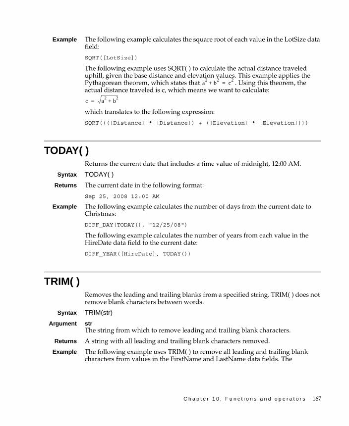
C h a p t e r 1 0 , F u n c t i o n s a n d o p e r a t o r s 167
Example The following example calculates the square root of each value in the LotSize data field:
SQRT([LotSize])
The following example uses SQRT( ) to calculate the actual distance traveled uphill, given the base distance and elevation values. This example applies the Pythagorean theorem, which states that . Using this theorem, the actual distance traveled is c, which means we want to calculate:
which translates to the following expression:
SQRT((([Distance] * [Distance]) + ([Elevation] * [Elevation])))
TODAY( )Returns the current date that includes a time value of midnight, 12:00 AM.
Syntax TODAY( )
Returns The current date in the following format:
Sep 25, 2008 12:00 AM
Example The following example calculates the number of days from the current date to Christmas:
DIFF_DAY(TODAY(), "12/25/08")
The following example calculates the number of years from each value in the HireDate data field to the current date:
DIFF_YEAR([HireDate], TODAY())
TRIM( )Removes the leading and trailing blanks from a specified string. TRIM( ) does not remove blank characters between words.
Syntax TRIM(str)
Argument strThe string from which to remove leading and trailing blank characters.
Returns A string with all leading and trailing blank characters removed.
Example The following example uses TRIM( ) to remove all leading and trailing blank characters from values in the FirstName and LastName data fields. The
a2 b2+ c2
=
c a2 b2+=

168 U s i n g A c t u a t e B I R T J a v a C o m p o n e n t s
expression uses the & operator to concatenate each trimmed FirstName value with a space, then with each trimmed LastName value.
TRIM([FirstName]) & " " & TRIM([LastName])
TRIMLEFT( )Removes the leading blanks from a specified string.
Syntax TRIMLEFT(str)
Arguments strThe string from which to remove the leading blank characters.
Returns A string with all leading blank characters removed.
Example The following example concatenates a literal string with each value in the customerName data field. TRIMLEFT( ) removes all blank characters preceding the customerName value so that there are no extra blank characters between the literal string and the customerName value.
"Customer name: " & TRIMLEFT([customerName])
TRIMRIGHT( )Removes the trailing blanks from a specified string.
Syntax TRIMRIGHT(str)
Argument strThe string from which to remove the trailing blank characters.
Returns A string with all trailing blank characters removed.
Example The following example concatenates each value in the Comment data field with a semicolon, then with a value in the Action data field. TRIMRIGHT( ) removes all blank characters after the Comment value so that there are no extra blank characters between the Comment string and the semicolon.
TRIMRIGHT([Comment]) & "; " & [Action]
UPPER( )Converts all letters in a string to uppercase.
Syntax UPPER(str)
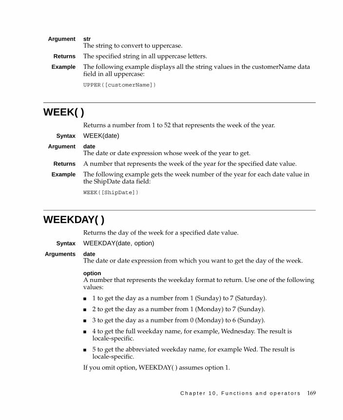
C h a p t e r 1 0 , F u n c t i o n s a n d o p e r a t o r s 169
Argument strThe string to convert to uppercase.
Returns The specified string in all uppercase letters.
Example The following example displays all the string values in the customerName data field in all uppercase:
UPPER([customerName])
WEEK( )Returns a number from 1 to 52 that represents the week of the year.
Syntax WEEK(date)
Argument dateThe date or date expression whose week of the year to get.
Returns A number that represents the week of the year for the specified date value.
Example The following example gets the week number of the year for each date value in the ShipDate data field:
WEEK([ShipDate])
WEEKDAY( )Returns the day of the week for a specified date value.
Syntax WEEKDAY(date, option)
Arguments dateThe date or date expression from which you want to get the day of the week.
optionA number that represents the weekday format to return. Use one of the following values:
■ 1 to get the day as a number from 1 (Sunday) to 7 (Saturday).
■ 2 to get the day as a number from 1 (Monday) to 7 (Sunday).
■ 3 to get the day as a number from 0 (Monday) to 6 (Sunday).
■ 4 to get the full weekday name, for example, Wednesday. The result is locale-specific.
■ 5 to get the abbreviated weekday name, for example Wed. The result is locale-specific.
If you omit option, WEEKDAY( ) assumes option 1.
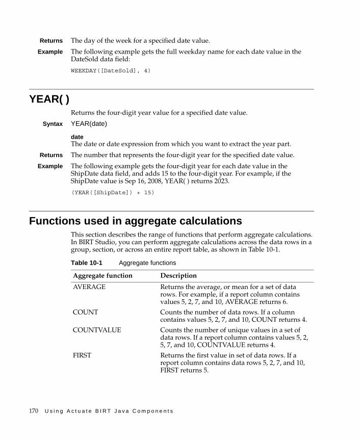
170 U s i n g A c t u a t e B I R T J a v a C o m p o n e n t s
Returns The day of the week for a specified date value.
Example The following example gets the full weekday name for each date value in the DateSold data field:
WEEKDAY([DateSold], 4)
YEAR( )Returns the four-digit year value for a specified date value.
Syntax YEAR(date)
dateThe date or date expression from which you want to extract the year part.
Returns The number that represents the four-digit year for the specified date value.
Example The following example gets the four-digit year for each date value in the ShipDate data field, and adds 15 to the four-digit year. For example, if the ShipDate value is Sep 16, 2008, YEAR( ) returns 2023.
(YEAR([ShipDate]) + 15)
Functions used in aggregate calculationsThis section describes the range of functions that perform aggregate calculations. In BIRT Studio, you can perform aggregate calculations across the data rows in a group, section, or across an entire report table, as shown in Table 10-1.
Table 10-1 Aggregate functions
Aggregate function Description
AVERAGE Returns the average, or mean for a set of data rows. For example, if a report column contains values 5, 2, 7, and 10, AVERAGE returns 6.
COUNT Counts the number of data rows. If a column contains values 5, 2, 7, and 10, COUNT returns 4.
COUNTVALUE Counts the number of unique values in a set of data rows. If a report column contains values 5, 2, 5, 7, and 10, COUNTVALUE returns 4.
FIRST Returns the first value in set of data rows. If a report column contains data rows 5, 2, 7, and 10, FIRST returns 5.
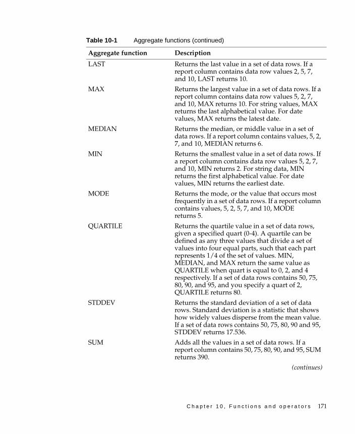
C h a p t e r 1 0 , F u n c t i o n s a n d o p e r a t o r s 171
LAST Returns the last value in a set of data rows. If a report column contains data row values 2, 5, 7, and 10, LAST returns 10.
MAX Returns the largest value in a set of data rows. If a report column contains data row values 5, 2, 7, and 10, MAX returns 10. For string values, MAX returns the last alphabetical value. For date values, MAX returns the latest date.
MEDIAN Returns the median, or middle value in a set of data rows. If a report column contains values, 5, 2, 7, and 10, MEDIAN returns 6.
MIN Returns the smallest value in a set of data rows. If a report column contains data row values 5, 2, 7, and 10, MIN returns 2. For string data, MIN returns the first alphabetical value. For date values, MIN returns the earliest date.
MODE Returns the mode, or the value that occurs most frequently in a set of data rows. If a report column contains values, 5, 2, 5, 7, and 10, MODE returns 5.
QUARTILE Returns the quartile value in a set of data rows, given a specified quart (0-4). A quartile can be defined as any three values that divide a set of values into four equal parts, such that each part represents 1/4 of the set of values. MIN, MEDIAN, and MAX return the same value as QUARTILE when quart is equal to 0, 2, and 4 respectively. If a set of data rows contains 50, 75, 80, 90, and 95, and you specify a quart of 2, QUARTILE returns 80.
STDDEV Returns the standard deviation of a set of data rows. Standard deviation is a statistic that shows how widely values disperse from the mean value. If a set of data rows contains 50, 75, 80, 90 and 95, STDDEV returns 17.536.
SUM Adds all the values in a set of data rows. If a report column contains 50, 75, 80, 90, and 95, SUM returns 390.
(continues)
Table 10-1 Aggregate functions (continued)
Aggregate function Description
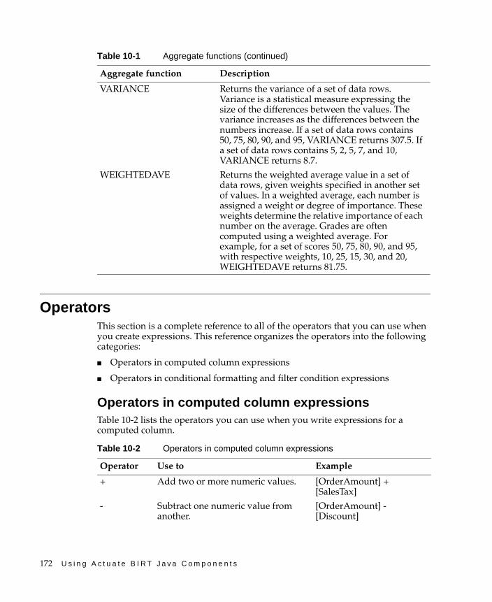
172 U s i n g A c t u a t e B I R T J a v a C o m p o n e n t s
OperatorsThis section is a complete reference to all of the operators that you can use when you create expressions. This reference organizes the operators into the following categories:
■ Operators in computed column expressions
■ Operators in conditional formatting and filter condition expressions
Operators in computed column expressionsTable 10-2 lists the operators you can use when you write expressions for a computed column.
VARIANCE Returns the variance of a set of data rows. Variance is a statistical measure expressing the size of the differences between the values. The variance increases as the differences between the numbers increase. If a set of data rows contains 50, 75, 80, 90, and 95, VARIANCE returns 307.5. If a set of data rows contains 5, 2, 5, 7, and 10, VARIANCE returns 8.7.
WEIGHTEDAVE Returns the weighted average value in a set of data rows, given weights specified in another set of values. In a weighted average, each number is assigned a weight or degree of importance. These weights determine the relative importance of each number on the average. Grades are often computed using a weighted average. For example, for a set of scores 50, 75, 80, 90, and 95, with respective weights, 10, 25, 15, 30, and 20, WEIGHTEDAVE returns 81.75.
Table 10-1 Aggregate functions (continued)
Aggregate function Description
Table 10-2 Operators in computed column expressions
Operator Use to Example
+ Add two or more numeric values. [OrderAmount] + [SalesTax]
- Subtract one numeric value from another.
[OrderAmount] - [Discount]

C h a p t e r 1 0 , F u n c t i o n s a n d o p e r a t o r s 173
Operators in conditional formatting and filter condition expressionsTable 10-3 lists the operators you can use when you create expressions for conditional formatting and filter conditions.
* Multiply numeric values. [Price] * [Quantity]
/ Divide numeric values. [Profit]/12
^ Raise a numeric value to a power. [Length]^2
% Specify a percent. [Price] * 80%
= Test if two values are equal. IF([ProductName] = "1919 Ford Falcon", "Discontinued Item", [ProductName])
> Test if one value is greater than another value.
IF([Total] > 5000, [Total]*15%, [Total]*10%)
< Test if one value is less than another value.
IF([SalePrice] < [MSRP], "Below MSRP", "Above MSRP")
>= Test if one value is greater than or equal to another value.
IF([Total] >= 5000, [Total]*15%, [Total]*10%)
<= Test if one value is less than or equal to another value.
IF([SalePrice] <= [MSRP], "Below or equal to MSRP", "Above MSRP")
<> Test if two values are not equal. IF([Country] <> "USA", "Imported product", "Domestic product")
AND Test if two or more conditions are true.
IF(([Gender] = "Male" AND [Salary] >= 150000 AND [Age] < 50), "Match found", "No match")
OR Test if any one of multiple conditions is true.
IF(([City] = "Boston") OR ([City] = "San Francisco"), "U.S.", "Europe and Asia")
& Concatenate string values. [FirstName] & " " & [LastName]
Table 10-2 Operators in computed column expressions
Operator Use to Example
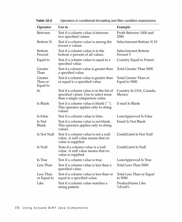
174 U s i n g A c t u a t e B I R T J a v a C o m p o n e n t s
Table 10-3 Operators in conditional formatting and filter condition expressions
Operator Use to Example
Between Test if a column value is between two specified values.
Profit Between 1000 and 2000
Bottom N Test if a column value is among the lowest n values.
SalesAmount Bottom N 10
Bottom Percent
Test if a column value is in the bottom n percent of all values.
SalesAmount Bottom Percent 5
Equal to Test if a column value is equal to a specified value.
Country Equal to France
Greater Than
Test if a column value is greater than a specified value.
Total Greater Than 5000
Greater Than or Equal to
Test if a column value is greater than or equal to a specified value.
Total Greater Than or Equal to 5000
In Test if a column value is in the list of specified values. Use to select more than a single comparison value.
Country In USA, Canada, Mexico
Is Blank Test if a column value is blank (" "). This operator applies only to string values.
E-mail Is Blank
Is False Test if a column value is false. LoanApproved Is False
Is Not Blank
Test if a column value is not blank. This operator applies only to string values.
Email Is Not Blank
Is Not Null Test if a column value is not a null value. A null value means that no value is supplied.
CreditLimit Is Not Null
Is Null Tests if a column value is a null value. A null value means that no value is supplied.
CreditLimit Is Null
Is True Test if a column value is true. LoanApproved Is True
Less Than Test if a column value is less than a specified value.
Total Less Than 5000
Less Than or Equal to
Test if a column value is less than or equal to a specified value.
Total Less Than or Equal to 5000
Like Test if a column value matches a string pattern.
ProductName Like %Ford%
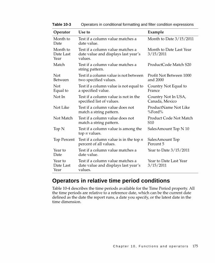
C h a p t e r 1 0 , F u n c t i o n s a n d o p e r a t o r s 175
Operators in relative time period conditionsTable 10-4 describes the time periods available for the Time Period property. All the time periods are relative to a reference date, which can be the current date defined as the date the report runs, a date you specify, or the latest date in the time dimension.
Month to Date
Test if a column value matches a date value.
Month to Date 3/15/2011
Month to Date Last Year
Test if a column value matches a date value and displays last year’s values.
Month to Date Last Year 3/15/2011
Match Test if a column value matches a string pattern.
ProductCode Match S20
Not Between
Test if a column value is not between two specified values.
Profit Not Between 1000 and 2000
Not Equal to
Test if a column value is not equal to a specified value.
Country Not Equal to France
Not In Test if a column value is not in the specified list of values.
Country Not In USA, Canada, Mexico
Not Like Test if a column value does not match a string pattern.
ProductName Not Like %Ford%
Not Match Test if a column value does not match a string pattern.
Product Code Not Match S10
Top N Test if a column value is among the top n values.
SalesAmount Top N 10
Top Percent Test if a column value is in the top n percent of all values.
SalesAmount Top Percent 5
Year to Date
Test if a column value matches a date value.
Year to Date 3/15/2011
Year to Date Last Year
Test if a column value matches a date value and displays last year’s values.
Year to Date Last Year 3/15/2011
Table 10-3 Operators in conditional formatting and filter condition expressions
Operator Use to Example
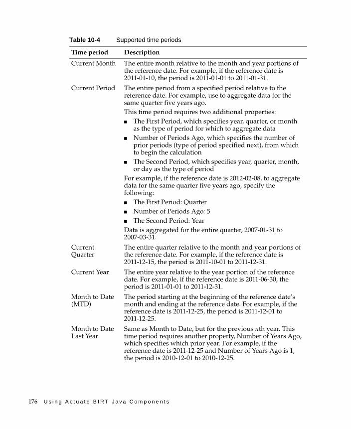
176 U s i n g A c t u a t e B I R T J a v a C o m p o n e n t s
Table 10-4 Supported time periods
Time period Description
Current Month The entire month relative to the month and year portions of the reference date. For example, if the reference date is 2011-01-10, the period is 2011-01-01 to 2011-01-31.
Current Period The entire period from a specified period relative to the reference date. For example, use to aggregate data for the same quarter five years ago.This time period requires two additional properties:■ The First Period, which specifies year, quarter, or month
as the type of period for which to aggregate data■ Number of Periods Ago, which specifies the number of
prior periods (type of period specified next), from which to begin the calculation
■ The Second Period, which specifies year, quarter, month, or day as the type of period
For example, if the reference date is 2012-02-08, to aggregate data for the same quarter five years ago, specify the following:■ The First Period: Quarter■ Number of Periods Ago: 5■ The Second Period: YearData is aggregated for the entire quarter, 2007-01-31 to 2007-03-31.
Current Quarter
The entire quarter relative to the month and year portions of the reference date. For example, if the reference date is 2011-12-15, the period is 2011-10-01 to 2011-12-31.
Current Year The entire year relative to the year portion of the reference date. For example, if the reference date is 2011-06-30, the period is 2011-01-01 to 2011-12-31.
Month to Date (MTD)
The period starting at the beginning of the reference date’s month and ending at the reference date. For example, if the reference date is 2011-12-25, the period is 2011-12-01 to 2011-12-25.
Month to Date Last Year
Same as Month to Date, but for the previous nth year. This time period requires another property, Number of Years Ago, which specifies which prior year. For example, if the reference date is 2011-12-25 and Number of Years Ago is 1, the period is 2010-12-01 to 2010-12-25.
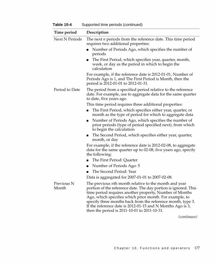
C h a p t e r 1 0 , F u n c t i o n s a n d o p e r a t o r s 177
Next N Periods The next n periods from the reference date. This time period requires two additional properties:■ Number of Periods Ago, which specifies the number of
periods■ The First Period, which specifies year, quarter, month,
week, or day as the period in which to begin the calculation
For example, if the reference date is 2012-01-01, Number of Periods Ago is 1, and The First Period is Month, then the period is 2012-01-01 to 2012-01-31.
Period to Date The period from a specified period relative to the reference date. For example, use to aggregate data for the same quarter to date, five years ago.This time period requires three additional properties:■ The First Period, which specifies either year, quarter, or
month as the type of period for which to aggregate data■ Number of Periods Ago, which specifies the number of
prior periods (type of period specified next), from which to begin the calculation
■ The Second Period, which specifies either year, quarter, month, or day
For example, if the reference date is 2012-02-08, to aggregate data for the same quarter up to 02-08, five years ago, specify the following:■ The First Period: Quarter■ Number of Periods Ago: 5■ The Second Period: YearData is aggregated for 2007-01-01 to 2007-02-08.
Previous N Month
The previous nth month relative to the month and year portion of the reference date. The day portion is ignored. This time period requires another property, Number of Months Ago, which specifies which prior month. For example, to specify three months back from the reference month, type 3. If the reference date is 2012-01-15 and N Months Ago is 3, then the period is 2011-10-01 to 2011-10-31.
(continues)
Table 10-4 Supported time periods (continued)
Time period Description
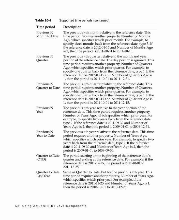
178 U s i n g A c t u a t e B I R T J a v a C o m p o n e n t s
Previous N Month to Date
The previous nth month relative to the reference date. This time period requires another property, Number of Months Ago, which specifies which prior month. For example, to specify three months back from the reference date, type 3. If the reference date is 2012-01-15 and Number of Months Ago is 3, then the period is 2011-10-01 to 2011-10-15.
Previous N Quarter
The previous nth quarter relative to the month and year portion of the reference date. The day portion is ignored. This time period requires another property, Number of Quarters Ago, which specifies which prior quarter. For example, to specify one quarter back from the reference date, type 1. If the reference date is 2012-03-15 and Number of Quarters Ago is 1, then the period is 2011-10-01 to 2011-12-31.
Previous N Quarter to Date
The previous nth quarter relative to the reference date. This time period requires another property, Number of Quarters Ago, which specifies which prior quarter. For example, to specify one quarter back from the reference date, type 1. If the reference date is 2012-03-15 and Number of Quarters Ago is 1, then the period is 2011-10-01 to 2011-12-15.
Previous N Year
The previous nth year relative to the year portion of the reference date. This time period requires another property, Number of Years Ago, which specifies which prior year. For example, to specify two years back from the reference date, type 2. If the reference date is 2011-09-30 and Number of Years Ago is 2, then the period is 2009-01-01 to 2009-12-31.
Previous N Year to Date
The previous nth year relative to the reference date. This time period requires another property, Number of Years Ago, which specifies which prior year. For example, to specify two years back from the reference date, type 2. If the reference date is 2011-09-30 and Number of Years Ago is 2, then the period is 2009-01-01 to 2009-09-30.
Quarter to Date (QTD)
The period starting at the beginning of the reference date’s quarter and ending at the reference date. For example, if the reference date is 2011-12-25, the period is 2011-10-01 to 2011-12-25.
Quarter to Date Last Year
Same as Quarter to Date, but for the previous nth year. This time period requires another property, Number of Years Ago, which specifies which prior year. For example, if the reference date is 2011-12-25 and Number of Years Ago is 1, then the period is 2010-10-01 to 2010-12-25.
Table 10-4 Supported time periods (continued)
Time period Description
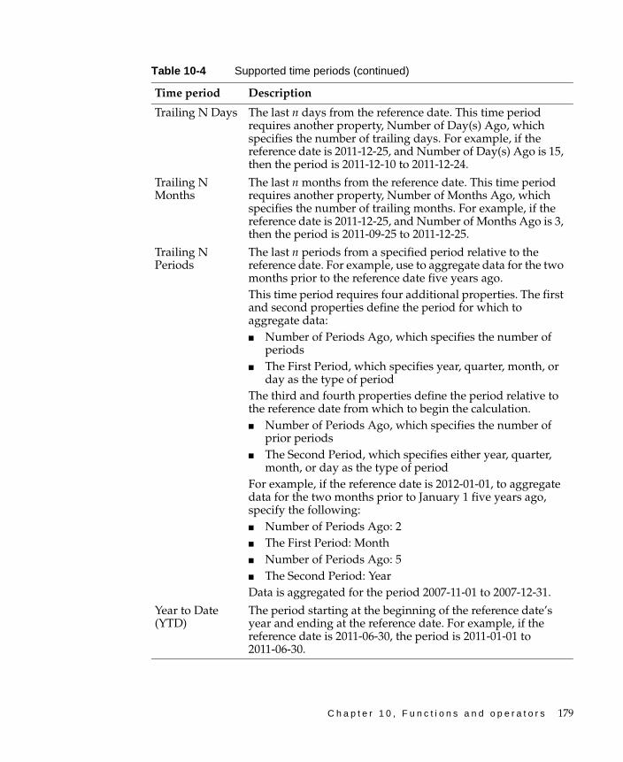
C h a p t e r 1 0 , F u n c t i o n s a n d o p e r a t o r s 179
Trailing N Days The last n days from the reference date. This time period requires another property, Number of Day(s) Ago, which specifies the number of trailing days. For example, if the reference date is 2011-12-25, and Number of Day(s) Ago is 15, then the period is 2011-12-10 to 2011-12-24.
Trailing N Months
The last n months from the reference date. This time period requires another property, Number of Months Ago, which specifies the number of trailing months. For example, if the reference date is 2011-12-25, and Number of Months Ago is 3, then the period is 2011-09-25 to 2011-12-25.
Trailing N Periods
The last n periods from a specified period relative to the reference date. For example, use to aggregate data for the two months prior to the reference date five years ago.This time period requires four additional properties. The first and second properties define the period for which to aggregate data:■ Number of Periods Ago, which specifies the number of
periods■ The First Period, which specifies year, quarter, month, or
day as the type of periodThe third and fourth properties define the period relative to the reference date from which to begin the calculation.■ Number of Periods Ago, which specifies the number of
prior periods■ The Second Period, which specifies either year, quarter,
month, or day as the type of periodFor example, if the reference date is 2012-01-01, to aggregate data for the two months prior to January 1 five years ago, specify the following:■ Number of Periods Ago: 2■ The First Period: Month■ Number of Periods Ago: 5■ The Second Period: YearData is aggregated for the period 2007-11-01 to 2007-12-31.
Year to Date (YTD)
The period starting at the beginning of the reference date’s year and ending at the reference date. For example, if the reference date is 2011-06-30, the period is 2011-01-01 to 2011-06-30.
Table 10-4 Supported time periods (continued)
Time period Description

180 U s i n g A c t u a t e B I R T J a v a C o m p o n e n t s
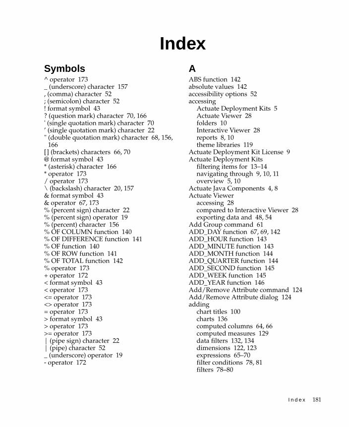
I n d e x 181
IndexSymbols^ operator 173_ (underscore) character 157, (comma) character 52; (semicolon) character 52! format symbol 43? (question mark) character 70, 166' (single quotation mark) character 70’ (single quotation mark) character 22" (double quotation mark) character 68, 156,
166[] (brackets) characters 66, 70@ format symbol 43* (asterisk) character 166* operator 173/ operator 173\ (backslash) character 20, 157& format symbol 43& operator 67, 173% (percent sign) character 22% (percent sign) operator 19% (percent) character 156% OF COLUMN function 140% OF DIFFERENCE function 141% OF function 140% OF ROW function 141% OF TOTAL function 142% operator 173+ operator 172< format symbol 43< operator 173<= operator 173<> operator 173= operator 173> format symbol 43> operator 173>= operator 173| (pipe sign) character 22| (pipe) character 52_ (underscore) operator 19- operator 172
AABS function 142absolute values 142accessibility options 52accessing
Actuate Deployment Kits 5Actuate Viewer 28folders 10Interactive Viewer 28reports 8, 10theme libraries 119
Actuate Deployment Kit License 9Actuate Deployment Kits
filtering items for 13–14navigating through 9, 10, 11overview 5, 10
Actuate Java Components 4, 8Actuate Viewer
accessing 28compared to Interactive Viewer 28exporting data and 48, 54
Add Group command 61ADD_DAY function 67, 69, 142ADD_HOUR function 143ADD_MINUTE function 143ADD_MONTH function 144ADD_QUARTER function 144ADD_SECOND function 145ADD_WEEK function 145ADD_YEAR function 146Add/Remove Attribute command 124Add/Remove Attribute dialog 124adding
chart titles 100charts 136computed columns 64, 66computed measures 129data filters 132, 134dimensions 122, 123expressions 65–70filter conditions 78, 81filters 78–80
182 U s i n g A c t u a t e B I R T J a v a C o m p o n e n t s
adding (continued)formatting rules 32, 34, 37page breaks 58, 63
addition 171Advanced Filter dialog box 81, 82, 84Advanced Sort command 60Advanced Sort dialog box 60aggregate data 128
adding 71, 72calculating values for 170comparing 94deleting 73displaying 70, 75, 110entering labels for 72exporting 53grouping data and 70recalculating 78
aggregate functions 71listed 170
Aggregate on property 72aggregating data 70–73aggregation 137Aggregation command 71Aggregation dialog box 71, 72, 73Alignment command 138analyzing data 48, 61AND operator 83, 173Angle option (charts) 101animation properties 48Any Of operator 81applications 6Arrange Columns dialog box 58, 63ascending sort order 60, 122asterisk (*) character 166attributes
filtering 133Auto format option 138AVERAGE function 170axes values (charts)
filtering 98plotting 99
Bbackground colors 99backslash (\) character 20, 22, 157banner (Actuate Development Kit) 10
bar charts 88bar colors 99bar stick stock chart subtypes 94BETWEEN function 146Between operator 19, 174BIDI text 49BIRT data design 12BIRT data designs 12BIRT Deployment Kit 9, 16
See Actuate Deployment KitsBIRT Designer Professional
applying themes and 119BIRT Interactive Crosstabs 4BIRT Interactive Viewer 4, 9BIRT reports 16
See also reportsBIRT Studio 4, 9
applying themes and 119BIRT Viewer 4blank characters 167, 168Boolean column format dialog box 40Boolean data type 40Boolean expressions 40, 153, 157, 159Bottom N operator 174Bottom Percent operator 174brackets ([]) characters 66, 70browser-based tools
See also web browsersbubble charts 96buttons 18
Ccalculated data 53, 64, 129, 140calculations 70, 129candlestick stock chart subtypes 94capitalization 168case 157, 168case sensitivity
pattern matching 156category series 88, 99, 102CEILING function 147changing
chart subtypes 98chart titles 137charts 88, 98cross tabs 117
I n d e x 183
default settings 16filter conditions 84reports 27, 32sort order 13summary tables 85
character filters 14character formats 41, 43character patterns 19character strings. See stringscharacters
as literal values 20converting to lowercase 43converting to uppercase 43counting 156creating expressions and 70finding matching 156, 157, 166flat file formats and 52, 54QBE expressions and 19removing leading or trailing 167, 168
Chart Builder 136chart elements 53chart legends 101, 102, 106chart reports 88Chart size option 100Chart Subtype dialog box 98chart subtypes 101chart titles 100, 101, 137chart types 88, 137chart views 106charts
applying themes to 100changing 98creating 136, 137displaying data and 88displaying multiple value series in 137displaying small sets of values in 91, 94drilling through 102editing 88exporting 51overlapping series in 90selecting subtype 101showing percentages in 89, 90showing relationships in 92, 93showing scheduling information in 95showing scientific or statistical data 93showing side-by-side series in 88stacking series in 88, 90
tracking financial data and 96tracking stock data and 93viewing 136viewing series values in 101, 107
check boxes 18Classic Models.data file 112closing values 94colors 32, 99column areas (cross tabs) 110column charts 89column headers
collapsing data groups and 75exporting data and 54selecting 32
column menu icon 28columns
accessing toolbar for 28adding computed measures to 129adding dimensions to cross tab 122, 123aggregating data and 70, 71, 72applying conditional formats to 34, 37comparing values in 35, 36copying formats for 44deleting 58, 59displaying calculated data and 129displaying data type of 38displaying hidden 59exporting specific 53filtering data in 133filtering merged 85formatting data in 32, 38generating summary values for 128grouping data and 61, 63, 118grouping on multiple 63hiding 59pivoting 127removing aggregate data from 73removing dimensions from 123resizing 59, 118selecting 32setting page breaks for 63sorting data in 60sorting multiple 60sorting values in 121, 122suppressing duplicate values in 75, 76testing values in 174
comma (,) character 52
184 U s i n g A c t u a t e B I R T J a v a C o m p o n e n t s
comma-separated values files 52comparison operators 34, 79, 82
filters and 133comparisons
aggregate values 94filtering data and 133grouping data and 61literal values 35multiple columns and 35multiple values and 35, 81
computed column names 66computed columns
building expressions for 65, 66, 68calculating values for 140, 172creating 64, 66
Computed Measure dialog 129computed measures
creating 129displaying calculated data and 129generating values for 130
concatenation 67concatenation operator 173conditional expressions 34, 35, 153conditional format operators 173conditional formatting 32–37Conditional Formatting command 33Conditional Formatting dialog box 33, 34, 35conditional formatting rules 32, 34, 37conditions
calculating values and 153comparing data and 34, 35, 82testing 173
cone charts 96Copy Format command 44Copy Format dialog box 44copying
formats 44COUNT function 170COUNTVALUE function 170creating
charts 136, 137computed columns 64, 66computed measures 129expressions 65–70filter conditions 78, 81, 133filters 78–80, 132, 134formatting rules 32, 34, 37
reports 5cross tab elements 117cross tabs
adding dimensions 122, 123calculating values in 129changing 117displaying data and 110displaying details about 119drilling through 125exporting 48, 51formatting data in 117formatting in 117hiding elements in 125, 126organizing data in 121pivoting data in 127reducing the size of 125resizing columns and rows in 118size limitation for 125switching views for 107viewing 110
.csv files 52CSV files 52cube view files 12cubes 110Currency format 39currency values 39, 41current date and time 160, 167customizing
charts 98, 99, 137cross tabs 117date-and-time formats 42numeric formats 41reports 27string formats 43summary tables 85
Ddashboard gadgets 52dashboards 16, 91data
aggregating 70–73, 137analyzing 48, 61displaying 58, 59, 88, 125, 126exporting 52–55filtering 17, 18, 58, 85, 98formatting 32, 38

I n d e x 185
grouping 17, 61–63hiding 74, 125, 126organizing 58, 61, 121restoring original order of 60retrieving 16, 18selecting 32showing relationships among 92, 93showing trends in 93sorting 59, 59–60, 72, 121–122viewing information about 119viewing unexpected values for 37
data cubes 110data fields
adding to expressions 70testing for null values in 155
data hierarchies 125data hierarchy levels 121data points 88, 93, 99data ranges 146data rows
calculating running totals for 165counting 170returning first value in 170returning largest value in 171returning last value in 171returning mean value in 170returning most frequent value in 171returning smallest value in 171returning unique values for 170returning variance value for 172showing quartile value for 171
data seriesdisplaying relationship between 93displaying relationship to whole 92displaying values 101, 107drilling through 102, 104, 105hiding 106overlapping multiple 90plotting data and 88, 99showing distinct values for 91showing high and low values 94showing open and close values 94showing percentage of whole 89, 90showing side-by-side comparisons of 88showing variation between 95stacking multiple 88, 90
data sources 26filtering data in 17, 18retrieving data from 16, 18
data type export options 54data types 37Date column format dialog box 40date expressions 175date values
adding days to 69, 142adding months to 144adding quarters to 144adding time values to 143, 145adding weeks to 145adding years to 146as literals 68calculating days between 148calculating months between 149calculating quarters between 150calculating time values between 148, 149,
151calculating weeks between 151calculating years between 152comparing 35creating charts and 95exporting data and 54formatting 42–43grouping 61, 62plotting 99restoring default formats for 44returning current 160, 167returning month for 158returning quarter in 160returning weekdays for 147, 169returning weeks for 169returning year for 170subtracting 69
date-and-time format symbols 42date-and-time formats 39, 40, 42date-and-time functions 67DAY function 147Day Of Year level 131days
adding to date values 69, 142calculating number of 148returning number in month 147returning specific 169
186 U s i n g A c t u a t e B I R T J a v a C o m p o n e n t s
decimal separators 68decimal values 38, 41default settings 16default values 17Delete Column command 59deleting
aggregate data 73blank characters 167, 168columns 58, 59dimensions 123filter conditions 84filter selections 14page breaks 64report files 13
delimiter characters 52, 54deployment kits. See Actuate Deployment
Kitsdescending sort order 60, 122designs 5, 16detail areas (cross tabs) 110detail data 74, 75, 125details icon 10deviation 95dials 91DIFF_DAY function 67, 69, 148DIFF_HOUR function 148DIFF_MINUTE function 149DIFF_MONTH function 149DIFF_QUARTER function 150DIFF_SECOND function 151DIFF_WEEK function 151DIFF_YEAR function 152difference charts 95dimensions 110
adding to cross tabs 122, 123deleting 123filtering values in 133plotting data and 137reordering 123sorting 121, 122
Disable Interactivity command 28displaying
aggregate values 70, 75, 110BIRT data designs 12calculated values 64, 128, 129, 140charts 106, 136
columns 59cross tabs 110cube view files 12data 58, 59, 88, 125, 126distinct values 91filter conditions 81hidden values 76numeric values 38PDF output 52report elements 73report files 10, 13, 14reports 5, 16, 26, 28series values 101, 107subfolders 14summary values 171table of contents 61tables 106tooltips 119unique values 170XHTML documents 52
distinct values 91Do Not Repeat Values command 76documentation vii, 9documents 14, 16
See also reportsdisplaying data and 26exporting specific pages 51
Documents link 10Documents page 9, 10, 13double quotation mark (") character 68, 156,
166doughnut charts 93DPI settings
AFP output 49Drill Down command 125Drill Up command 125Drill Up Or Drill Down dialog 126drilling 125drilling actions
standard charts 102, 104, 105drop-down lists 18duplicate values
hiding 75, 76meter charts and 91
dynamic filter operators 18dynamic filter parameters 18
I n d e x 187
Ee.reports
See also reportsemitters 48Enable Interactivity command 28Encoding Style property 54Equal to operator 19, 174Excel emitters 48Excel formats
exporting report content and 48, 51, 52, 54Excel spreadsheets 48executable files 4, 14, 16exponents 39Export Column Data Type option 54Export Column Display Name option 54Export Column Header option 54Export Column Name option 54Export Content dialog box
PDF output formats and 50Export Data command 53Export Data dialog box 53Export Data With Carriage Return option 54Export Locale Neutral Format option 54export options 48exporting
cross tabs 48, 51data 52–55Flash charts 52Flash gadgets 52images 51report content 48–52specific report pages 51standard charts 51
exporting restrictions 53expression builder 65expressions 18, 19
adding 65–70adding reserved characters to 70aggregating data and 71calculating data values and 65, 140, 172creating 65–70creating computed columns and 66, 68creating computed measures and 130field names in 66filtering data and 78, 82, 173formatting data and 34, 35, 40, 173
literal values in 68negating Boolean 159returning unexpected values from 37See also QBE expressionsselecting values for 35verifying data types in 38verifying syntax of 68
extensible HTML formats 48, 52
Ffield names 66, 70fields
adding to expressions 70creating expressions and 65, 66displaying specific set of 78sorting data and 59testing for null values in 155
file links 16file lists 13file menu 11file systems 5file types 12files
See also specific typeaccessing 10deleting 13displaying 10, 13, 14exporting and 48, 52, 54filtering 14managing 5saving output 51selecting 16
files and folders page 5See also Documents page
Filter command 133filter conditions
adding 78changing 84creating 133creating multiple 81deleting 84displaying 81grouping 81, 83selecting multiple values for 80, 82
Filter dialog 133Filter dialog box 79, 81, 84
188 U s i n g A c t u a t e B I R T J a v a C o m p o n e n t s
filter expressions 18, 19, 173Filter icon 133Filter options 10filtering
data 17, 18, 58, 85, 98items on Deployment Kit pages 13–14
filters 14creating 78–80, 132, 134removing 84setting on merged columns 85testing 80
filters selections 14financial data 96FIND function 152FIRST function 170Fixed format 39Flash charts 88
exporting 48, 52printing 52
Flash gadgetsexporting 52printing 52
flat file formatsexporting report content and 48, 52, 54
folder links 10folders
accessing 10displaying 14filtering contents 14removing files from 13viewing contents 10, 13, 14viewing details about 10, 11
Font command 138Font dialog box 138font size 99fonts 99footers 72Format Chart command 101Format Chart dialog box 101Format command 117, 138Format Data command 38format patterns 41, 42, 43formats
copying 44creating multiple rules for 37defining custom 41, 42, 43exporting report data and 48, 52
selecting standard 38, 39, 41setting conditions for 32–37
formattingBoolean values 40data 32, 38text 32, 41–43
formatting options 34, 117formatting rules 32, 34, 37function categories (expression builder) 65functions 66, 68, 140
mathematical operations and 130
Ggadgets 52
exporting data only 52–55Gantt charts 95General Date format 40General Number format 38generating reports 16glass styles (charts) 101Greater Than operator 174Greater than operator 19Greater Than or Equal to operator 174Greater than or equal to operator 19Group Details dialog box 62group footers 72group headers 72, 75, 76grouping
data 61–63filter conditions 83
grouping data 17grouping intervals 62groups 128, 137
aggregating data and 70, 72changing order of 63collapsing and expanding 75displaying data and 61displaying date-and-time values in 61, 62formatting cross tabs and 118hiding detail data in 74, 75hiding duplicate values in 75, 76removing page breaks from 64selecting multiple columns and 63setting page breaks for 63sorting values in 72
GUIs. See graphical user interfaces
I n d e x 189
Hheaders
displaying aggregate data in 72suppressing duplicate values and 75, 76
Hide Column command 59Hide Detail command 75Hide or Show Items dialog box 73hiding
detail data 74, 75, 125, 126duplicate values 75, 76HTML5 chart series data 106items in reports 59, 73summary data 126
hierarchies 125hierarchy levels 121home folders 10horizontal bar charts 88hours
adding to date values 143calculating number of 148
HTML formatsexporting report content and 51exporting reports and 48, 52
HTML5 chartshiding data in 106
IIf expressions 34IF function 67, 153images
exporting 51immediate jobs 16IN function 154In operator 19, 174input 16Interactive Crosstabs
calculating data values and 128hiding data and 126
interactive features 26Interactive Viewer 4, 9
accessing 28calculating data and 65changing reports and 32, 58compared to Actuate Viewer 28customizing charts and 88, 98displaying date values and 42
displaying reports and 27, 58displaying summary tables and 85exporting data and 48filtering data and 78formatting data and 37, 38, 44grouping data and 61hiding duplicate values and 75hiding report elements and 73starting 28
Interval option (charts) 101interval types (groups) 62Is Blank operator 174Is False operator 174Is false operator 19Is Not Blank operator 174Is Not Null operator 174Is not null operator 19Is Null operator 174Is null operator 19Is True operator 174Is true operator 19ISNULL function 155
JJava Components. See Actuate Java
Componentsjobs 16
Llabels
adding aggregate data and 72adding calculated data and 66creating computed measures and 130formatting chart 99selecting 32
landing pages 4, 9LAST function 171leading characters 167, 168LEFT function 155legend titles (charts) 101legends 102, 106LEN function 156Less Than operator 174Less than operator 19Less than or equal operator 19Less Than or Equal to operator 174
190 U s i n g A c t u a t e B I R T J a v a C o m p o n e n t s
levels 121libraries (theme) 119library files 119licenses 9, 28LIKE function 156Like operator 19, 174line charts 90links 9, 10, 16listing reports 70lists 13, 18, 35
testing for values in 154literal characters 157literal values 20, 35, 68locales
creating computed columns and 68exporting data and 54formatting date-and-time values for 39, 42formatting numeric values for 38viewing bidirectional text and 49
logical functions 67logical operators 83Long Date format 40Long Time format 40LOWER function 157lowercase characters 41, 43, 157Lowercase format 41
MMATCH function 157Match operator 19, 175matching character patterns 156, 157, 166mathematical functions 130mathematical operations 67, 172MAX function 171MAX_PAGE_SIZE parameter 125measures 110
creating computed 129filtering data in 133plotting data and 137
MEDIAN function 171Medium Date format 40Medium Time format 40menus 10metacharacters 19meter charts 91, 99MIN function 171
minutesadding to date values 143calculating number of 149
MOD function 158MODE function 171modulus 158MONTH function 158Month to Date Last Year operator 175Month to Date operator 175months
adding to date values 144calculating number of 149returning 158
Move to Group Header command 76Move to Group Header dialog box 77multipage reports 28, 58multiple sort actions 60multiple-value parameters 17, 18
Nnames
reserved characters in 70naming
computed columns 66naming computed measures 130negating Boolean expressions 159networked environments 4New Computed Column command 66New Computed Column dialog box 66New Computed Measure icon 129No Condition operator 19None setting 122non-null values 159, 174Not Between operator 175Not between operator 19Not Equal to operator 175Not equal to operator 19NOT function 159Not In operator 175Not in operator 19Not Like operator 175Not like operator 19Not Match operator 175Not match operator 19NOTNULL function 159NOW function 160
I n d e x 191
null values 155, 174Number column format dialog box 39numeric data types 38numeric formats 38, 39, 41numeric values
aggregating 170as literals 68calculating percentage of 140, 141, 142calculating ratio for 161calculating running totals for 165calculating square root of 166comparing 35displaying 38formatting 38–41grouping 61plotting 99restoring default formats for 44returning absolute 142returning difference between 141returning modulo value for 158rounding 147, 163, 164showing relationship between 88
OOn Detail Row option 115online documentation. See documentationopening
Actuate Deployment Kits 9Actuate Viewer 27document files 16Interactive Viewer 28Java Components application 8
opening values 94operators 133
calculating data and 66comparing data and 34filter expressions 18filtering data and 82types listed 172
optional parameters 17OR operator 173output 16output formats
bidirectional text and 49exporting report data and 48, 52
Oversize page limitation 125
PPage Break command 63Page Break dialog box 63, 64page breaks 58, 63pagination 51, 58parameter types 17parameters
filtering data with 18retrieving data and 78retrieving data with 16, 18running jobs and 16setting values for 17
Parameters page 16, 17passwords 17pattern matching 19, 156, 157, 166PDF emitters 48, 51PDF formats
bidirectional printing and 49exporting Flash objects and 48, 52exporting report content and 48, 50, 51
% OF COLUMN function 140% OF DIFFERENCE function 141% OF function 140% OF ROW function 141% OF TOTAL function 142percent (%) character 156Percent format 39percent stacked chart subtypes 89, 90percentages 39, 67, 173
displaying calculated data and 140, 141, 142
pie charts 92, 99pipe (|) character 52pipe-separated values files 52, 54Pivot icon 127pivoting cross tabs 127PostScript emitters 52PostScript formats
bidirectional printing and 49exporting and 48, 52
PowerPoint formatsexporting and 48, 51
predefined themes (charts) 100predefined values 17presentations 32
192 U s i n g A c t u a t e B I R T J a v a C o m p o n e n t s
printingFlash objects 52
project scheduling information 95properties
animation 48exporting data and 48, 51formatting data and 32
PSV files 52, 54public folders 10publishing themes 119pyramid charts 96
QQUARTER function 160quarters 144, 150, 160QUARTILE function 171queries. See QBE expressionsquestion mark (?) character 70, 166quotation mark characters. See double
quotation mark; single quotation mark characters
Rradar charts 94radio buttons 18range of values 146, 161RANK function 161RATIO function 161Recalculate Totals option 132recalculating aggregate data 78regular expressions 19relationships (data) 92, 93removing
dimensions 123Reorder Columns command 58, 63Repeat Values command 76report components 26report designs 5, 16report documents 14, 16
displaying data and 26exporting specific pages 51
report elements 26, 32, 73report emitters 48report executables. See report object
executable filesreport file types 12
report filesSee also specific typeaccessing 10deleting 13displaying 10, 13, 14exporting and 48, 52, 54filtering 14managing 5selecting 16
report items 73report library files 119report object executable files 14
See also executable filesreport parameter values files 17report parameters. See parametersreport viewers 4, 26, 28
See also specific viewerreporting tasks 28reports
accessing 8, 10adding aggregate data to 70adding calculated data to 66, 70changing 32controlling content of 58creating 5customizing 27displaying 5, 16, 26, 28distributing information and 4exporting content 48–52exporting data 52–55filtering data and 80generating 16grouping data and 61, 63, 74hiding data in 74hiding items in 59, 73removing page breaks from 64retrieving data for 16, 18running 16setting page breaks for 58, 63viewing data in 58, 80
repository 5requests. See jobsrequired parameters 17reserved characters 70resizing
columns 59, 118rows 118
I n d e x 193
result sets 52return values 37, 65RIGHT function 162ROUND function 163ROUNDDOWN function 164rounding 147, 163, 164ROUNDUP function 164row areas (cross tabs) 110rows
aggregating data and 70, 72calculating running totals for 165counting 170displaying specific set of 58, 79exporting specific 54filtering data in 133generating summary values for 128grouping data and 61hiding duplicate values in 75, 76pivoting 127resizing 118returning first value in 170returning largest value in 171returning last value in 171returning mean value in 170returning most frequent value in 171returning smallest value in 171returning unique values for 170returning variance value for 172setting page breaks for 63showing quartile value for 171sorting values in 121, 122
.rox files. See report object executable files
.rptdesign files. See report designs
.rptdocument files. See report documentsRun page 16run requests. See jobsrunning
jobs 16reports 16
running totals 165RUNNINGSUM function 165
Ssaving
PDF output 51scalable vector graphics 51
scatter charts 93scheduling information 95Scientific format 39scroll bars 101SEARCH function 165searching
data sources 19searching text strings 152, 165seconds
adding to date values 145calculating number of 151
sectors (pie charts) 92Select Data Item dialog box 85Select Values dialog box 35Select Values link 133semicolon (;) character 52semicolon-separated values files 52, 54series
displaying relationship between 93displaying relationship to whole 92displaying values 101, 107overlapping multiple 90showing distinct values for 91showing high and low values 94showing open and close values 94showing percentage of whole 89, 90showing side-by-side comparisons of 88showing variation between 95stacking multiple 88, 90
Short Date format 40Short Time format 40Show Column command 59Show Detail command 75Show Detail Tooltip command 119side menu 10side-by-side bar chart subtypes 88single quotation mark (') character 70single quotation mark (’) character 22single-value parameters 17slider bars (charts) 107Sort command 122Sort dialog 122sort order 13, 59, 60, 122sorting data 59, 59–60, 72, 121–122special characters 156, 166spider radar chart subtypes 94spreadsheets 48
194 U s i n g A c t u a t e B I R T J a v a C o m p o n e n t s
SQRT function 166square root 166SSV files 52, 54stacked chart subtypes 88, 89, 90Stagger option (charts) 101standard deviation 171standard meter chart subtypes 91starting
Actuate Viewer 27Interactive Viewer 28
STDDEV function 171Step option (charts) 101stock charts 93String column format dialog box 41string data types 38string format symbols 43string formats 41, 43string patterns 156, 157, 166strings
comparing values for 35concatenating 67, 173converting to lowercase 43, 157converting to uppercase 43, 168counting characters in 156finding substrings in 152, 165formatting values 32, 38grouping data and 61matching characters in 156, 157matching set of characters in 19removing blank characters in 167, 168restoring default formats for 44returning length of 156returning substrings in 155, 162
subfolders 14submitting jobs 16substrings
extracting 155, 162finding location of 152, 165
subtotals 61, 128SUM function 171summary data 70, 88, 110, 171
calculating percentages of 140, 141, 142displaying 128, 129drilling through 125hiding 126
summary reports 61, 74
summary tablescustomizing 85
superimposed meter chart subtypes 91suppressing duplicate values 76SVG formats 51Switch View command 106syntax errors (expressions) 70
Ttab character 52table elements 53table footers 70, 72table headers 70, 72table of contents 61table views 106tables
aggregating data and 70, 72displaying 106exporting specific columns in 53, 54exporting specific rows in 54formatting data in 32hiding columns in 59hiding duplicate values in 75, 76removing aggregate data from 73resizing columns in 59selecting columns in 32selecting report elements in 32
tab-separated values files 52, 54text
formatting 32, 41–43plotting 99restoring default formats for 44
text files 52, 54text patterns 19theme libraries 119themes
creating charts and 100time formats 39, 40, 42time functions 67time line slider bars (charts) 107time range selectors (charts) 107time values
adding to date values 143, 145calculating number of 148, 149, 151creating charts and 90, 95, 107exporting data and 54
I n d e x 195
formatting 42–43grouping 61, 62restoring default formats for 44returning current 160, 167
titles 100, 137TODAY function 167toolbars 28tooltips 119Top N operator 175Top Percent operator 175totals 78, 165
displaying 128returning percentage of 140, 141, 142
trailing characters 167, 168trends 93TRIM function 167TRIMLEFT function 168TRIMRIGHT function 168TSV files 52, 54tube charts 96Type page (Chart Builder) 137types. See data types
Uunderscore (_) character 157Unformatted format option 44Unformatted option 138unique values 170unscheduled jobs 16upgrades 26UPPER function 168uppercase characters 41, 43, 168Uppercase format 41URLs 8user names 17user selection lists 18
Vvalue series 88, 99, 104, 105values
See also dataassigning to parameters 17calculating 70, 129comparing 35, 61, 81determining rank 161determining variance in 172
determining weighted average for 172displaying distinct 91displaying unique 170formatting Boolean 40formatting on 33, 34, 35, 37grouping data and 61hiding duplicate 75, 76negating Boolean 159retrieving specific 18returning difference between 141returning from expressions 37, 65returning largest 171returning median 171returning most frequent 171returning percentages for 140, 141, 142returning ratio for 161returning smallest 171returning unexpected 37selecting 35showing over time 90showing relationship between 88showing relationships between 93showing variation between 95testing for non-null 159testing if null 155testing range of 146
VARIANCE function 172viewers 4, 26, 28
See also specific viewerviewing
aggregate values 70, 75, 110BIRT data designs 12calculated values 64, 128, 129, 140charts 106, 136columns 59cross tabs 110cube view files 12data 58, 59, 88, 125, 126distinct values 91filter conditions 81hidden values 76numeric values 38PDF output 52report elements 73report files 10, 13, 14reports 5, 16, 26, 28series values 101, 107
196 U s i n g A c t u a t e B I R T J a v a C o m p o n e n t s
viewing (continued)subfolders 14summary values 171table of contents 61tables 106tooltips 119unique values 170XHTML documents 52
viewing environments 26views, switching between 106
Wweb browsers 5web.xml 125WEEK function 169WEEKDAY function 169weekdays
adding to date values 69, 142calculating number of 148returning number in month 147returning specific 169
weeksadding to date values 145calculating number of 151returning 169
WEIGHTEDAVE function 172wildcard characters 14, 156, 166Word document formats 48, 51
Xx-axis labels 101x-axis titles 101x-axis values 99XHTML emitters 52XHTML formats 48, 52xls formats 48xlsx formats 48, 51
Yy-axis labels 101y-axis titles 101y-axis values 99, 101YEAR function 170Year to Date Last Year operator 175Year to Date operator 175years
adding to date values 146calculating number of 152returning 170