USING A DYNAMIC ARTIFICIAL NEURAL NETWORK · PDF fileperceptrón multicapa y un modelo ARCH para pronosticar la varianza condicional ... modelos no lineales; heterocedasticidad. Using

Revista Ingenierías Universidad de Medellín

Revista Ingenierías Universidad de Medellín, vol. 12, No. 22 pp. 127 - 136 - ISSN 1692 - 3324 - enero-junio de 2013/204 p. Medellín, Colombia

USING A DYNAMIC ARTIFICIAL NEURAL NETWORK FOR FORECASTING THE VOLATILITY OF A FINANCIAL TIME SERIES*

Juan D. Velásquez**

Sarah Gutiérrez1***

Carlos J. Franco****

Recibido: 08/02/2012Aceptado: 07/05/2013

ABSTRACTThe ability to obtain accurate volatility forecasts is an important issue for the

financial analyst. In this paper, we use the DAN2 model, a multilayer perceptron and an ARCH model to predict the monthly conditional variance of stock prices. The results show that DAN2 model is more accurate for predicting in-sample and out-of-sample variance that the other considered models for the used dataset. Thus, the value of this neural network as a predictive tool is demonstrated.

Keywords: Volatility forecast; prediction; nonlinear models; heteroskedasticity.

* Artículo de investigación científica y tecnológica.** Doctor en Ingeniería, Área de Sistemas Energéticos, Universidad Nacional de Colombia, Medellín, Colombia (2009); Magíster en Ingeniería

de Sistemas, Universidad Nacional de Colombia, Medellín, Colombia (1997); Profesor Asociado de la Universidad Nacional de Colombia (sede Medellín, Colombia).. Dirección de correspondencia: Universidad Nacional de Colombia. Facultad de Minas. Medellín, Colombia. Correo electrónico: [email protected]. Autor de correspondencia.

*** Ingeniera de Sistemas, Universidad Nacional de Colombia, sede Medellín, Colombia (2011) Dirección de correspondencia: Universidad Nacional de Colombia. Facultad de Minas. Medellín, Colombia. Correo electrónico: [email protected]

**** Doctor en Ingeniería-Área Sistemas Energéticos, Universidad Nacional de Colombia, sede Medellín, Colombia (2002); Magíster en Aprove-chamiento de Recursos Hidráulicos, Universidad Nacional de Colombia, sede Medellín, Colombia (1996). Profesor Asociado de la Universidad Nacional de Colombia (sede Medellín, Colombia). Dirección de correspondencia: Universidad Nacional de Colombia. Facultad de Minas. Medellín, Colombia. Correo electrónico: [email protected].

128 Juan D. Velásquez - Sarah Gutiérrez - Carlos J. Franco

Universidad de Medellín

USO DE UNA RED NEURONAL ARTIFICIAL DINÁMICA PARA PRONOSTICAR LA VOLATILIDAD DE UNA SERIE DE TIEMPO

FINANCIERA

RESUMENLa habilidad para obtener pronósticos precisos de la volatilidad es un importante

problema para el analista financiero. En este artículo, se usa el modelo DAN2, un perceptrón multicapa y un modelo ARCH para pronosticar la varianza condicional mensual de una acción. Los resultados muestran que el modelo DAN2 es más pre-ciso para pronosticar las varianzas dentro-de-la-muestra y fuera-de-la-muestra que los otros modelos considerados para el conjunto de datos utilizado. Así, el valor de esta red neuronal como herramienta predictiva es demostrado.

Palabras clave: pronóstico de la volatilidad; modelos no lineales; heterocedasticidad.

129Using a dynamic artificial neural network for forecasting the volatility of a financial time series


INTRODUCTION The ability to obtain accurate volatility forecasts is an important issue for the financial analyst, due to the necessity of performing risk management, evaluating option prices and conducting hedging strategies [1-6]. Since the seminal work of Engle [7], several heteroskedastic parametric models have been proposed for representing the struc-ture of volatility in return series, including: the GARCH model of Bollerslev [8], the A-GARCH, NA-GARCH and V-GARCH models of Engle and Ng [9], the Quadratic ARCH model of Sentana [10], the A-PARCH of Ding, Granger and Engle [11], and the Augmented GARCH model of Duan [12], among others.

All of previous models are parametric and their equation is predefined, such that, it is only necessary to estimate suitable values for the param-eters. However, this is only an approach to the real dynamics of the variance in the studied times series and the use of artificial neural networks has been gain popularity for forecasting volatility in the last two decades; this is due to their capacity of learning the “hidden” relationships in the data without the necessity of supposing a particular parametric mod-el. Several representative works about this topic are described as follows; Malliaris and Salchenberger [13] forecast the implied volatility of S&P100 using a multilayer perceptron; Ormoneit and Neuneier [14] compare the performance of multilayer percep-trons and density estimating neural network when the volatility and the returns of the German Stock Index DAX are predicted. Donalson and Kamstra [15] propose a new hybrid model for conditional volatility by adding a multilayer perceptron and a GJR-GARCH model; the proposed model is used to forecast the volatility of stock volatility in S&P500, NIKKEY, FTSE and TSEC international market indices outperforming GJR, GARCH and EGARCH models. González–Miranda and Burgess [16] predict the implied volatility from the Ibex35 index option using a multilayer perceptron neural network concluding that neural networks ordinary

dominates traditional linear models on the basis of out-of-sample dataset. Meissner and Kawano [17] train four types of artificial neural networks (mul-tilayer perceptron, radial basis functions network, probabilistic and generalized regression neural net-works) for forecasting the implied volatility of prices for ten high-tech stocks using as inputs the same data required for the Black-Scholes model; Meiss-ner and Kawano [17] find that the performance of multilayer perceptrons is significantly better than the Black-Scholes model. Wang [18] uses the volatility forecasts obtained using a GARCH, GJR-GARCH and Grey-GJR–GARCH models as inputs for a multilayer perceptron. Tseng, Cheng, Wang and Peng [19] use a perceptron neural network to forecast the Taiwan stock index option prices us-ing the same inputs required for the Black-Scholes model. Lin and Yeh [20] use a backpropagation neural network (multilayer perceptron) to forecast Taiwan stock index option prices using, as in previ-ous cases, the same inputs of Black-Scholes model. Dhar, Agrawal, Singhal, Singh and Murmu [21] study the forecasting ability of multilayer percep-tron neural networks whose inputs are the same summands in classical volatility models.

Recently, a new dynamic neural network for time series forecasting, called DAN2, was proposed by Ghiassi and Saidane [22]; Ghiassi, Saidane and Zimbra [23] conclude that DAN2 is more accurate than other neural network models when several nonlinear benchmark time series are forecasted; similar conclusions are reported by Ghiassi, Said-ane and Zimbra [24] and Velásquez and Franco [25] in real world applications. However, there are not published experiences about the use of DAN2 for forecasting the historical volatility of financial time series.

The aim of this paper is to compare the accu-racy of DAN2, ARCH and multilayer perceptron neural network models when the volatility of a benchmark return series is forecasted. The remain-der of this paper is organized as follows. Section



2 outlines the DAN2 model and the dataset used for the experiment; next, we present the empirical results in Section 3. Finally, Section 4 presents the conclusions.

1 MATERIALS AND METHODS

1.1 ARCH model

In his seminal work, Engle [7] introduces the au-toregressive conditional heteroskedasticity (ARCH) model of order P for forecasting the conditional variance, σ2

t, of the return, rt, as a function of previous squared shocks, e2

t–p:

2 20

1

(1)P

t p t pp

eσ ω ω −=

= + ∑and the return is:

(2)t t t tr c e c σ ε= + = +

where E(rt) = c, with c ≠ 0. εt is a random variable following a normal standard distribution. Several conditions are imposed to the parameters ωp (p = 0, …, P) to ensure that the unconditional variance of et is finite and positive.

1.2 DAN2 model for time series prediction

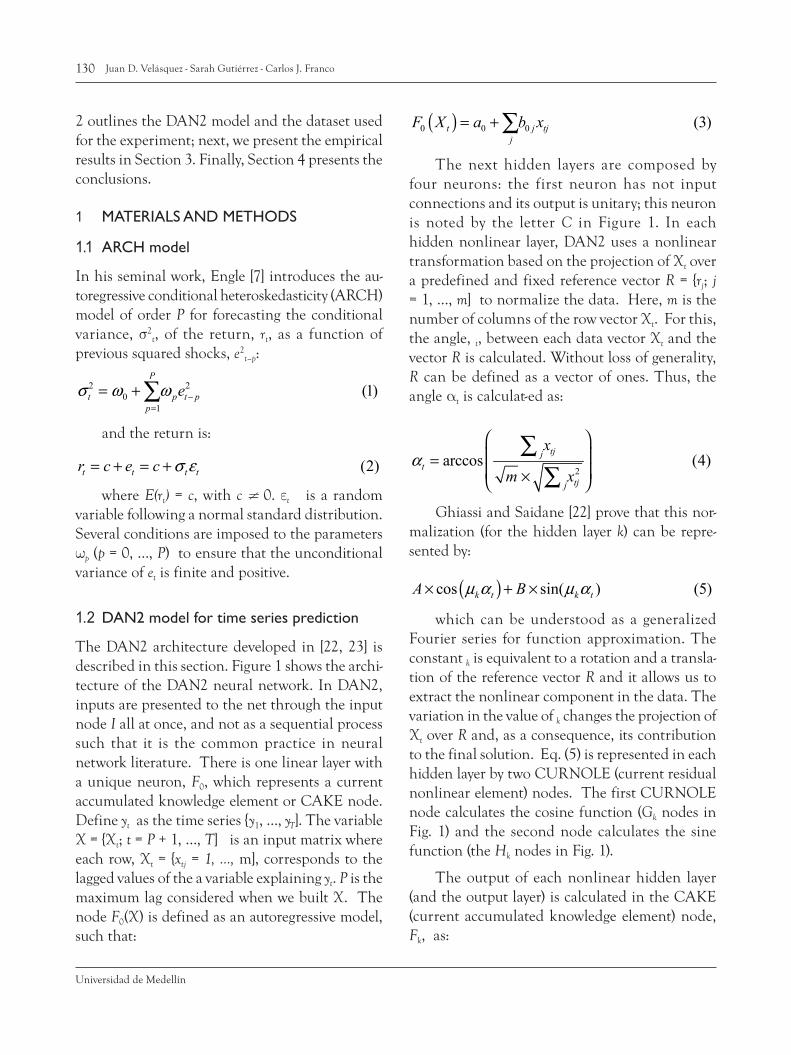
The DAN2 architecture developed in [22, 23] is described in this section. Figure 1 shows the archi-tecture of the DAN2 neural network. In DAN2, inputs are presented to the net through the input node I all at once, and not as a sequential process such that it is the common practice in neural network literature. There is one linear layer with a unique neuron, F0, which represents a current accumulated knowledge element or CAKE node. Define yt as the time series {y1, …, yT]. The variable X = {Xt; t = P + 1, …, T] is an input matrix where each row, Xt = {xtj = 1, …, m], corresponds to the lagged values of the a variable explaining yt. P is the maximum lag considered when we built X. The node F0(X) is defined as an autoregressive model, such that:

( )0 0 0 (3)t j tjj

F X a b x= + ∑The next hidden layers are composed by

four neurons: the first neuron has not input connections and its output is unitary; this neuron is noted by the letter C in Figure 1. In each hidden nonlinear layer, DAN2 uses a nonlinear transformation based on the projection of Xt over a predefined and fixed reference vector R = {rj; j = 1, …, m] to normalize the data. Here, m is the number of columns of the row vector Xt. For this, the angle, t, between each data vector Xt and the vector R is calculated. Without loss of generality, R can be defined as a vector of ones. Thus, the angle αt is calculat-ed as:

2arccos (4)

tjjt

tjj

x

m xα

= ×

∑∑

Ghiassi and Saidane [22] prove that this nor-malization (for the hidden layer k) can be repre-sented by:

( )cos sin( ) (5)k t k tA Bµ α µ α× + ×

which can be understood as a generalized Fourier series for function approximation. The constant k is equivalent to a rotation and a transla-tion of the reference vector R and it allows us to extract the nonlinear component in the data. The variation in the value of k changes the projection of Xt over R and, as a consequence, its contribution to the final solution. Eq. (5) is represented in each hidden layer by two CURNOLE (current residual nonlinear element) nodes. The first CURNOLE node calculates the cosine function (Gk nodes in Fig. 1) and the second node calculates the sine function (the Hk nodes in Fig. 1).

The output of each nonlinear hidden layer (and the output layer) is calculated in the CAKE (current accumulated knowledge element) node, Fk, as:



( ) ( ) ( )( )

1 cos

sin (6)k t k k k t k k t

k k t

F X a b F X c

d

µ α

µ α−= + + +

where ak represents the weight associated to the C node; ck and dk are the weights associated to the CURNOLE nodes; Fk–1(Xt) is the output of the previous layer, and it is weighted by bk. Eq. (6) defines that the result of each layer is a weighted sum of the knowledge accumulated in the previous layer, Fk–1(Xt), the nonlinear transformation of Xt (Gk and Hk nodes) and a constant (the C node).

1.3 DAN2 model for volatility forecasting

DAN2 for time series prediction is described by equations (3), (4) and (6). It is straight forward to use DAN2 to predict the conditional volatility of returns following the same idea of ARCH models in eq. (1). For this, we assume that:

( ){ }

2

2

max{ , }

; 1, , , 0 (7)t K t

t t p

F X with

X e p P

σ δ

δ−

=

= = … >

Where K is the number of layers of DAN2; δ is a tolerance parameters to ensure that the condi-tional variance is always positive.

1.4 Intel data set

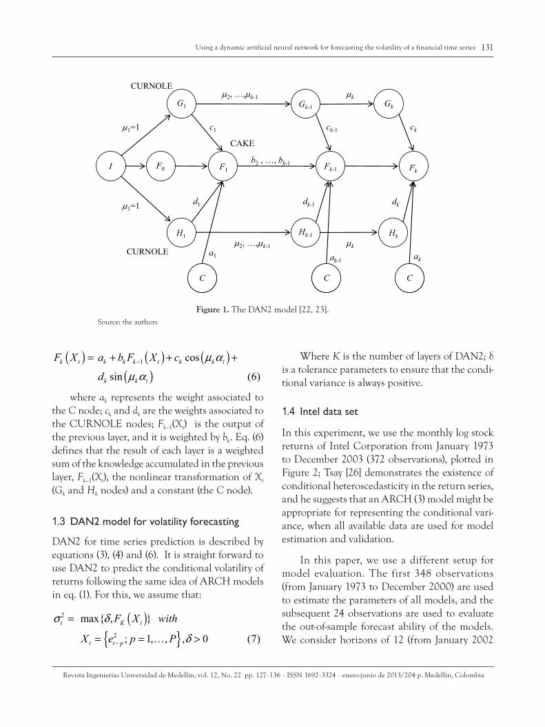
In this experiment, we use the monthly log stock returns of Intel Corporation from January 1973 to December 2003 (372 observations), plotted in Figure 2; Tsay [26] demonstrates the existence of conditional heteroscedasticity in the return series, and he suggests that an ARCH (3) model might be appropriate for representing the conditional vari-ance, when all available data are used for model estimation and validation.

In this paper, we use a different setup for model evaluation. The first 348 observations (from January 1973 to December 2000) are used to estimate the parameters of all models, and the subsequent 24 observations are used to evaluate the out-of-sample forecast ability of the models. We consider horizons of 12 (from January 2002

F0

CC CC CC

I

CURNOLE

CURNOLE

CAKE

b2 , …, bk-1F1 Fk-1 Fk

G1 Gk-1 Gk

HkHk-1H1

1=1

1=1

2, …,k-1

2, …,k-1

k

k

dkdk-1d1

a1 ak-1 ak

ckck-1c1

Figure 1. The DAN2 model [22, 23].Source: the authors



to December 2002) and 24 (from January 2002 to December 2003) months ahead.

2 RESULTS AND DISCUSSION In this section, we present and discuss the ob-tained results. The parameters for all models were estimated by maximizing the natural logarithm of the likelihood function of shocks:

22

21

( )log log 22

1 log (8)2

Tt

tt P t

T PL

e

π

σσ= +

−= −

− + ∑

In eq. (8), T is the number of observations used for parameter estimation. The performance of the considered models is measured using two criteria: the sum of squared errors (SSE):

22 2 (9)t tSSE e σ= −∑

And the sum of absolute errors:

2 2 (10)t tSAE e σ= −∑with et = rt – c. Here, rt are the monthly log

stock returns, c is a constant, et are the residuals or shocks, and σ2

t are the forecasted variances. Since the actual variance is unobservable, we use e2

t as a proxy in equations (9) and (10). Following the work of Tsay [25], we use the first three lags as inputs for all considered models.

In our work, we consider several DAN2 con-figurations differing in the number of processing layers and the same inputs for all models; thus, we train models from one to four hidden layers. Obtained results are summarized in Table 1. As benchmark models, we use an ARCH model and a multilayer perceptron neural network (MLP) using the same inputs of DAN2. We train a MLP with H = 1, 2, 3 and 4 neurons in the hidden layer, and

Figure 2. Monthly log stock returns of Intel Corporation from January 1973 to December 2003.Source: the authors



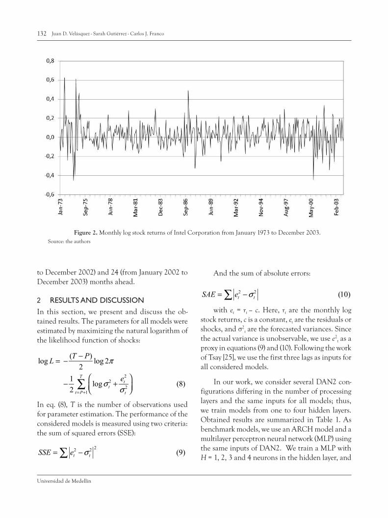
we prefer the model with lower values of SSE (SAE) for the forecast horizon.

Our analysis is the following:

• MLP is better than the ARCH model in pre-dict the variance of the studied time series; for training and forecasting horizons, artificial neural networks have lower values of SSE (SAE) than ARCH model; we consider that it is an indirect evidence that the presence of a nonlinear deterministic behavior that is not captured by the ARCH model.

• Parameter estimation by maximizing the log L function in eq. (8) is not equivalent to minimize the in-sample sum of squared forecast errors; this is due to the necessity of estimating the c parameter in eq. (2) together the parameters of the variance model. As is expected, the log L function increases con-

ModelTraining SSE

(SAE)

Forecasting SSE (SAE)12 months

ahead

Forecasting SSE (SAE)24 months

ahead

ARCH0.5053

(6.4482)0.0223 (0.3501)

0.0256 (0.5121)

MLP (H = 2)0.4859

(6.2605)0.0172

(0.3017)0.0210

(0.4911)

DAN2 (K=1)0.5142

(6.3792)0.0178

(0.3187)0.0210

(0.4795)

DAN2 (K=2)* 0.4707 (6.1693)

0.0201 (0.3560)

0.0225 (0.4729)

DAN2 (K=3)0.4885 (6.1972)

* 0.0148 (0.2809)

* 0.0185 (0.4440)

DAN2 (K=4)0.4658 (0.6913)

0.0205 (0.3253)

0.0227 (0.4414)

* Minimum values

Table 1. Obtained results

Source: the authors

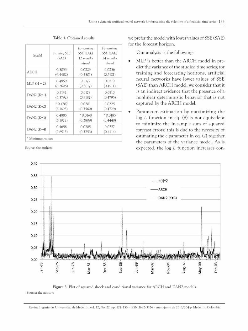
Figure 3. Plot of squared shock and conditional variance for ARCH and DAN2 models.Source: the authors



tinuously with the number of processing layers for the DAN2 model (224.83, 231.84, 234.32, 239.43 for K = 1, …, 4 respectively); however, the SSE calculated for the fitting sample does not decrease continuously with the number of layers; we found a local maximum of SSE forK = 3. Possibly, it is due to assumption of c ≠ 0 in eq. (2).

• DAN2 has better training and forecasting SSE respect to competitive models (ARCH and MLP). We prefer the DAN2 (K = 3) model, considering only forecast errors. The improve-ment gains in forecasting SSE by the DAN2 model are 67% and 72% when we consider the ARCH model as the reference model.

Finally, we plot the squared shocks and the con-ditional variance forecasts obtained with ARCH and DAN2 (K = 3) models (Figure 3) for the entire dataset. DAN2 seems to follow better the changes in the values of shocks than the ARCH model; in addition, forecasted values seem to be very different for both models.

3 CONCLUSIONSIn this paper, we use an artificial neural network with dynamic architecture to predict the volatility of Intel Corporation returns and we compare the obtained results with the predictions calculated using an ARCH model and a multilayer percep-tron neural network. The comparative assessment against the traditional models shows that DAN2 is more accurate. The obtained results encourage further research about the use of this new kind of neural network for forecasting volatility in financial time series.

There are several ways to extend this research. First, it is necessary to evaluate model performance for other return series; second; we do not con-sider the use of exogenous variables to explain the changes in volatility; and third, it is necessary to determinate if DAN2 would be valuable for fore-casting implied volatility in option pricing.

REFERENCES

[1] S.A. Hamid and Z. Iqbal, “Using neural networks for forecasting volatility of S&P 500 index futures prices”, Journal of Business Research, vol. 57, no. 10, pp. 1116-1125, 2004.

[2] L.-B. Tang, L.-X. Tang and H.-Y. Sheng, ”Forecasting volatility based on wavelet support vector machine”. Expert Systems with Applications, vol. 36, no. 2, part 2, pp. 2901-2909, 2009.

[3] T.E. Day and C.M. Lewis, “The behavior of the volatil-ity implicit in the prices of stock index options”. Journal of Financial Economics, vol. 22, no. 1, pp. 103–122, 1988.

[4] C.R. Harvey and R.E. Whaley, “S&P100 index option volatility”. Journal of Finance, vol. 46, no. 4, pp. 1551-1561, 1991.

[5] J. Hull and A. White, “The pricing of options on assets with stochastic volatilities”. Journal of Finance, vol. 42, no. 2, pp. 281-300, 1987.

[6] J.M. Poterba, and L.H. Summers, “The persistence of volatility and stock market fluctuations”. American Economic Review, vol. 76, no. 5, pp. 1142–1151, 1986.

[7] R.F. Engle, “Autoregressive conditional heteroskedastic-ity with estimates of the variance of United Kingdom inflations”. Econometrica, vol. 50, no. 4, pp. 987-1007, 1982.

[8] T. Bollerslev, “Generalized autoregressive conditional heteroskedasticity”. Journal of Econometrics, vol. 31, no. 3, pp. 307-327, 1986.

[9] R.F. Engle, and V. Ng, “Measuring and testing the impact of news on volatility”. Journal of Finance, vol. 48, no. 5, pp. 1747-1778, 1993.

[10] E. Sentana, “Quadratic ARCH models”. Review of Economic Studies, vol. 62, no. 4, pp. 639-661, 1995.

[11] Z. Ding, C.W.J. Granger and R.F. Engle, “A long memory property of stock market returns and a new model”. Journal of Empirical Finance, vol. 1, no. 1, pp. 83-106, 1993.

[12] J.C. Duan, “Augmented GARCH(P, Q) process and its diffusion limit”. Journal of Econometrics, vol. 79, no. 1, pp. 97-127, 1997.

[13] M. Malliaris and L. Salchenberger, “Using neural networks to forecast the S&P100 implied volatility”. Neurocomputing, vol. 10, no. 2, 183-195, 1996.

[14] D. Ormoneit, and R. Neuneier, “Experiments in pre-dicting the German Stock Index DAX with density



estimating neural networks”. Proc 1996 Conf Comput Intell Financ Eng (CIFEr), pp. 66–71, 1996.

[15] R.G. Donaldson and M. Kamstra, “An artificial neural network-GARCH model for international stock return volatility”. Journal of Empirical Evidence, vol. 4, no. 1, pp. 17-46, 1997.

[16] F. Gonzáles-Miranda and N. Burgess, “Modeling market volatilities: the neural network perspective”. European Journal of Finance, vol. 3, no. 2, pp. 137-57, 1997.

[17] G. Meissner and N. Kawano, “Capturing the volatil-ity smile of options on high-tech stocks-a combined GARCH-neural network approach”. Journal of Econom-ics and Finance, vol. 25, no. 3, pp. 276-293, 2001.

[18] Y.–H. Wang, “Nonlinear neural network forecasting model for stock index option price: hybrid GJR-GARCH approach”. Expert Systems with Applications, vol. 36, no. 1, pp. 564-570, 2009.

[19] C.-H. Tseng, S.-T. Cheng, Y.-H. Wang and J.-T. Peng, “Ar-tificial neural network model of the hybrid EGARCH volatility of the Taiwan stock index option prices”. Physica A, vol. 387, no. 13, pp. 3192-3200, 2008.

[20] C.-T. Lin and H.-Y. Yeh, “Empirical of the Taiwan stock index option price forecasting model – applied artificial

neural network”. Applied Economics, vol. 41, no. 15, pp. 1965-1972, 2009.

[21] J. Dhar, P. Agrawal, V. Singhal, A. Singh and R.Kr. Murmu, “Comparative Study of Volatility Forecasting between ANN and Hybrid Models for Indian Market”. International Research Journal of Finance and Economics, vol 45, pp. 68-79, 2010.

[22] M. Ghiassi and H. Saidane, “A dynamic architecture for artificial neural networks”. Neurocomputing, vol. 63, no. 2, pp. 397-413, 2005.

[23] M. Ghiassi, H. Saidane and D. K. Zimbra, “A dynamic artificial neural network model for forecasting time series events”. International Journal of Forecasting, vol. 21, no. 2, pp. 341-362, 2005.

[24] M. Ghiassi, D. K. Zimbra and H. Saidane, “Medium term system load forecasting with dynamic artificial neural network model”. Electric Power Systems Research, vol. 76, no. 5, pp. 302-316, 2006.

[25] J.D. Velásquez and C.J. Franco, “Prediction of the prices of electricity contracts using a neuronal network with dynamic architecture”. Innovar Journal, vol. 20, no. 36, pp. 7-14, 2010.

[26] R.S. Tsay, “Analysis of Financial Time Series”. Wiley-Interscience, 2010.

Documents

USING A DYNAMIC ARTIFICIAL NEURAL NETWORK · PDF fileperceptrón multicapa y un modelo ARCH para pronosticar la varianza condicional ... modelos no lineales; heterocedasticidad. Using