USER’S GUIDE TO

Fuzzy-Set / Qualitative Comparative Analysis

Charles C. Ragin Department of Sociology

University of California, Irvine Irvine, CA

cragin@uci.edu

Assisted by: Tyson Patros

Sarah Ilene Strand Claude Rubinson

July 2017 fsQCA and this manual are updated every few months.

Both can be downloaded from www.fsqca.com.

Based on: fsQCA 3.0 Copyright © 1999-2003, Charles Ragin and Kriss Drass Copyright © 2004-2017, Charles Ragin and Sean Davey

CONTENTS Chapter 1. Data Files A) Opening a Data File ………………………………………………………... 1 B) Opening Data Files of Various Formats ………………...…………………. 1 Excel SPSS Stata

Word / Notepad C) Saving File Options ………………………………………………………… 2 D) Opening fsQCA Data in Other Formats …………………………………... 3 SPSS Stata

Excel Chapter 2. Data Editor A) Entering Data ………………………………………………………………. 5 Variable Names Number of Cases B) Editing Data ………………………………………………………………... 7 Add / Delete Variables …………………………………………………... 7 Compute Variables………………………………………………………. 11 Recode Variables ………………………………………………………... 11 1) Recode Variables Into Same Variables 2) Recode Variables Into Different Variables Calibrating Fuzzy Sets..………………………………….………………. 13 Add / Insert Cases ……………………………………………………….. 15 Delete Cases ……………………………………………………………... 15 Select Cases If …………………………………………………………… 16 C) Working with Output ………………………………………………………. 17 Printing Documents Saving Results Chapter 3. Basic Procedures, Descriptive Statistics, and Graphs A) Necessary Conditions ……………………………………………………... 18 Obtaining Necessary Conditions Sample Output

B) Set Coincidence ………………………………………………………….... 20 Obtaining Set Coincidence Sample Output C) Subset/Superset Analysis …………………………………………………. 21 Obtaining Subset/Superset Analysis Sample Output

D) Descriptives ………………………………………………………………. 23 Obtaining Descriptive Statistics Sample Output E) XY Plot …………………………………………………………………… 24 Obtaining XY Plots Sample Output Chapter 4. Crisp-Set Analysis

A) Basic Concepts …………………………………………………………... 27 1) Use of Binary Data 2) Boolean Negation 3) Use of Truth Tables to Represent Data 4) Groupings 5) Boolean Addition 6) Boolean Multiplication 7) Combinatorial Logic Minimization …………………………………………………….………… 31 1) Use of Prime Implicants ………………………………………...…… 33 2) Use of De Morgan’s Law ……………………………………………. 35 3) Necessary and Sufficient Causes …………………………………….. 36 B) Data ………………………………………………………………………... 37 C) Analysis ……………………………………………………………………. 37 Truth Table Algorithm……………………………………………………. 38 Specify Analysis …………………………………………………………. 41 Standard Analysis ………………………………………………………... 42 Limited Diversity and Counterfactual Analysis …………………………. 42 Chapter 5. Fuzzy-Set Analysis

A) Operations on Fuzzy Sets………………………………………...……. 46

Logical AND Logical OR Negation B) Fuzzy Sets, Necessity, and Sufficiency (Fuzzy Subset Relation)……... 48 C) Using the Fuzzy Truth Table Algorithm…………………………….…. 50 D) Data and Analysis..……………………………………………………. 50 E) “Specify Analysis” Option …………………………………..……..….. 55 F) “Standard Analysis” Option ………………………….………………... 56 G) Output for “Specify Analysis” Option ………………………………… 57 H) Output for “Standard Analysis” Option ……………………………….. 59 G) Consistency and Coverage …………………………………………….. 60

Page 1

Chapter 1. DATA FILES A) Opening a Data File FsQCA opens with the following window:

From the menu choose:

File Open

In the Open File dialog box, select the file you want to open. Click Open. B) Opening Data Files of Various Formats Data files come in a wide variety of formats, and the software is designed to handle the following:

• Comma-separated values (*.csv) or comma-delimited file, produced by Excel and other spreadsheet software

Page 2

• Space separated (*.txt) space delimited file, can be created in WORD or other word processing software and saved as text only

• Tab separated (*.dat) tab delimited file, can be created using SPSS and other

statistical software packages

• Raw data files (*.raw) generated by Stata (extension can be changed to *.csv if saved in the comma-delimited format).

The recommended formats are *.csv (Excel) and *.dat (SPSS). Please note that fsQCA makes the following assumptions about the structure of *.csv, *.dat and *.txt data files. First, and most important, fsQCA assumes that the cells in the first row of the spreadsheet contain variable names for their respective columns. Second, fsQCA assumes that the data begin in the second row of the spreadsheet and that each case is a single row. Finally, fsQCA assumes that each column contains cells of the same type of data. Data types can vary across columns, but they must be consistent within columns. Please remember to use very simple variables names, using only alphanumeric characters with no embedded punctuation or spaces. For example, “GNP1990” is OK, but “GNP 1990” and “GNP-1990” are not. • Opening / Saving data originally created in Excel: Save the Excel file in *.csv (Comma Separated Values) format. Make sure that the first row of the Excel data spreadsheet contains the variable names. Open in fsQCA. • Opening / Saving data originally created in SPSS: Save the SPSS file in *.dat (tab delimited) format or *.csv (Comma Separated Values) format. SPSS will ask you whether you want to “Write variable names to file.” Do not uncheck this option. • Opening / Saving data originally created in Stata: Save the Stata file in *.dta format and then go to File, Export, and choose file as Comma-separated data. In the new window, insert the file name for “Write to the file,” then for “Delimiter” choose Comma-separated format, and click Submit. In some versions of Stata you may need to rename the new *.dta file as a *.csv file. • Opening / Saving data originally created in Word / Notepad: Enter the data delimited by spaces. Make sure that the first line contains the variable names, also separated by spaces. Save the file in a *.txt (Text only) format, TXT (Text with Line Breaks), TXT (MS-DOS), or TXT (MS-DOS with Line Breaks). Open in fsQCA. C) Saving File Options From the menu choose:

File

Page 3

Save… The modified data file is saved, overwriting the previous version of the file of the same name and location. Or: To save a new data file or save data in a different format, from the menu choose: File Save As… The file will save in *.csv (Comma Separated Values) format. Enter a filename for the new data file. D) Opening fsQCA Data in Other Formats Once you have your data in the fsQCA program and have completed some preliminary analyses, you have the option to either edit the data in fsQCA (see Chapter 2), or edit your data with the help of software packages you may be more familiar with (e.g., SPSS or Excel). Similarly, you can either display the data graphically with the fsQCA program (see Chapter 3), or turn to SPSS, Stata or Excel for more elaborate graphical representations. If you choose SPSS, Stata or Excel for these operations, you need to save the fsQCA file and transfer it to the program of your choice. SPSS

In order to open fsQCA data in SPSS, save the fsQCA data spreadsheet in Comma-separated values (*.csv) or comma-delimited file. Make sure that the string variables in the fsQCA data file are written without spaces in between them (no embedded spaces are allowed)

In SPSS choose:

File Open Data… Open the fsQCA file you have just saved. SPSS will ask you several questions regarding your file. Check the following options: Does you text file match a predefined format? No How are your variables arranged? Delimited Are variable names included at the top of your file? Yes Line number that contains variable names 1 What is the decimal symbol? Period The first case of data begins with line number? 2 How are your cases represented? Each line represents a case How many cases do you want to import? All of the cases

Page 4

Which delimiters appear between variables? Comma What is the text qualifier? None Would you like to save this file format for future Y/N use? Would you like to paste the syntax? No Then click FINISH You can now edit the data and display it graphically in SPSS. In order to transfer the SPSS file back to fsQCA, see Chapter 1) B) SPSS. Stata In order to open fsQCA data in Stata, save the fsQCA data spreadsheet in Comma-

separated values (*.csv) or comma-delimited file. Make sure that the string variables in the fsQCA data file are written without spaces in between them (no embedded spaces are allowed)

In Stata, choose

File Import Text data created by a spreadsheet In the new window, browse for your *.csv file and, for “Delimiter,” choose

Comma-delimited data. You can now edit and use the data in Stata.

In order to transfer the Stata file back to fsQCA, see Chapter 1) B) Stata.

Excel

In order to open fsQCA data in Excel, save the fsQCA data spreadsheet in comma separated format (*.csv). Make sure that the string variables in the fsQCA data file are written without spaces in between them (no embedded spaces).

In Excel choose: File Open… Open the fsQCA file you have just saved. You can now edit the data and display it graphically in Excel. In order to transfer the Excel file back to fsQCA, see above.

Page 5

Chapter 2. DATA EDITOR A) Entering Data (creating a data file from scratch, in fsQCA) From the menu choose:

Variables Add… The Add Variable window will open.

Enter the variable name. The following rules apply to variable names:

• The length of the name cannot exceed fifteen characters. • Each variable name must be unique; duplication is not allowed. • Variable names are not case sensitive. The names NEWVAR, NewVAR and

newvar are all considered identical. • Variable names cannot include spaces or hyphens or punctuation. • Only alphanumeric characters may be used (0-9, a-Z)

Add the variable by clicking the OK button.

In addition to adding new variables, you can delete variables by highlighting the variable and clicking

Variables Delete… Now, from the menu choose: Cases Add…

Page 6

Note: In general, fsQCA is able to process a large number of cases. Yet, a main feature of fsQCA is that it deals with combinations of causal conditions; thus, adding more variables will influence computational time more than adding more cases. The number of possible combinations is 2 to the k power, where k is the number of causal conditions. As a rule of thumb, 10 or fewer causal conditions (i.e., 1024 possible combinations) is not a problem in terms of computational time. When dealing with more than 10 conditions, it is just a matter of the amount of time you are willing to wait for the program to do the analyses. Most applications use three to eight causal conditions. Enter the number of cases of your data set, press the Ok button, and the Data Sheet window will appear:

Enter the data values. You can enter data in any order. You can enter data by case or

by variable, for selected areas or individual cells. The active cell is highlighted with a darker color. When you select a cell and enter a data value, the value is displayed in the cell editor under the menu bar. Values can be numeric or string. Data values are not recorded until after you press Enter.

Before closing the Data Sheet you need to save it in order not to lose the entered

information.

Page 7

B) Editing Data

Add / Delete Variables

In order to add variables to an already existing Data Sheet, choose:

Variables Add…

Enter the variable name and press the OK button. In order to delete existing variables in the Data Sheet, highlight a cell in the variable

column you want deleted and choose: Variables

Delete…

Compute Variables

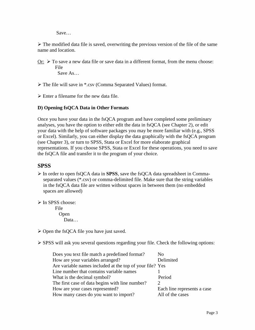
In order to compute new variables out of existing ones or numeric or logical expressions, choose:

Variables Compute…

The following window will open (with the names of the variables in your data file listed in the window on the left). [This chapter will use the example of countries with weak class voting from Ragin (2005)]:

Page 8

Type the name of a single target variable. It can be an existing variable or a new variable to be added to the working data file. Do not use a single letter as a variable name (e.g., “X”). This will cause the compute function to crash. Follow the variable

name guidelines on page 8.

To build an expression, either paste components into the Expression field or type directly in the Expression field (the window below the new variable field). 1) Arithmetic Operators

+ Addition. The preceding term is added to the following term.

Both terms must be numeric. - Subtraction. The following term is subtracted from the preceding

term. Both terms must be numeric. * Multiplication. The preceding and the following term are

multiplied. Both terms must be numeric. / Division. The preceding term is divided by the following term.

Both terms must be numeric, and the second must not be 0.

2) Relational Operators < Logical Less Than. True (=1) for numeric terms if the preceding

term is less than the following term. True for string terms if the preceding term appears earlier than the following term in the collating sequence (in alphabetical order). This operator is normally used only in a logical condition.

> Logical Greater Than. True (=1) for numeric terms if the

preceding term is greater than the following term. True for string terms if the preceding term appears later than the following term in the collating sequence (in alphabetical order). This operator is normally used only in a logical condition.

<= Logical Less Than Or Equal. True (=1) for numeric terms if the

preceding term is less or equal than the following term. True for string terms if the preceding term appears earlier than the following term in the collating sequence (in alphabetical order), or if the two are equal. This operator is normally used only in a logical condition.

>= Logical Greater Than Or Equal. True (=1) for numeric terms if

the preceding term is greater or equal than the following term. True for string terms if the preceding term appears later than the

Page 9

following term in the collating sequence (in alphabetical order), or if the two are equal. This operator is normally used only in a logical condition.

== Logical Equality. True (=1) for terms that are exactly equal. If

string terms are of unequal length, the shorter term is padded on the right with spaces before the comparison. This operator is normally used only in a logical condition.

!= Logical Inequality. True (=1) for terms that are not exactly equal.

If string terms are of unequal length, the shorter term is padded on the right with spaces before the comparison. This operator is normally used only in a logical condition.

&& Logical And. True (=1) if both the preceding and the following

term are logically true. The terms may be logical or numeric; numeric terms greater than 0 are treated as true. This operator is normally used only in a logical condition.

|| Logical Or. True if either the preceding or the following term are

logically true. The terms may be logical or numeric; numeric terms greater than 0 are treated as true. This operator is normally used only in a logical condition. This operator only works by pasting the symbol into the Expression Field.

~ Logical Not. True if the following term is false. 1 – (numeric

term). This operator is normally used only in a logical condition. 3) Arithmetic Functions

abs (x) Returns the absolute value of x, which must be numeric. acos (x) Returns the arc cosine (inverse function of cosine) of radians,

which must be a numeric value between 0 and 1, measured in radians.

asin (x) Returns the arc sine (inverse function of sine) of radians, which

must be a numeric value between 0 and 1, measured in radians. atan (x) Returns the arc tangent (inverse function of tangent) of radians,

which must be a numeric value, measured in radians. ceil (x) Returns the integer that results from rounding x up (x must be

numeric). Example: ceil (2.5) = 3.0

Page 10

calibrate Transforms an interval or ratio scale variable into a fuzzy set; see below for details.

cos (x) Return the cosine of radians, which must be a numeric value,

measured in radians. cosh (x) Returns the hyperbolic cosine [(ex + e-x)/2] of radians, which must

be a numeric value, measured in radians. X cannot exceed the value of 230.

exp (x) Returns e raised to the power x, where e is the base of the natural

logarithms and x is numeric. Large values of x (x > 230) produce results that exceed the capacity of the machine.

floor (x) Returns the integer that results from rounding x down (x must be

numeric). Example: floor (2.5) = 2.0

fmod (x,y) Returns the remainder when x is divided by modulus (y). Both

arguments must be numeric, and modulus must not be 0.

fuzzyand (x,…,) Returns the minimum of two or more fuzzy sets. Example: fuzzyand (1.0, 0.1) = 0.1

fuzzyor (x,…,) Returns the maximum of two or more fuzzy sets. Example: fuzzyor (1.0, 0.1) = 1.0 fuzzynot (x) Returns the negation (1-x) of fuzzy sets (same as Logical Not ‘~’). Example: fuzzynot (0.8) = 0.2 int (x) Returns the integer part of x. Numbers are rounded down to the

nearest integer. log (x) Returns the base-e logarithm of x, which must be numeric and

greater than 0. log10 (x) Returns the base-10 logarithm of x, which must be numeric and

greater than 0. pow (x,y) Returns the preceding term raised to the power of the following

term. If the preceding term is negative, the following term must be an integer. This operator can produce values too large or too small for the computer to process, particularly if the following term (the exponent) is very large or very small.

Page 11

round (x) Returns the integer that results from rounding x, which must be numeric. Numbers ending in .5 exactly are rounded away from 0.

Example: round (2.5) = 3.0 sin (x) Returns the sine of radians, which must be a numeric value,

measured in radians. sinh (x) Returns the hyperbolic sine [(ex - e-x)/2] of radians, which must be

a numeric value, measured in radians. X cannot exceed the value of 230.

square (x) Returns the square of x, which must be numeric. sqrt (x) Returns the positive square root of x, which must be numeric and

not negative. tan (x) Returns the tangent [sine/cosine] of radians, which must be a

numeric value, measured in radians. tanh (x) Returns the hyperbolic tangent [(ex – e-x) / (ex + e-x)] of radians,

which must be a numeric value, measured in radians. 4) Other Operators

( ) Grouping. Operators and functions within parentheses are evaluated before operators and functions outside the parentheses.

" Quotation Mark. Used to indicate the values of string variables. Example: Compute if….: Variable == “NA” SYSMIS System Missing. Used when selecting subsets of cases. Example: Select if...: Variable == SYSMISS Clear Deletes the text in the Expression Field.

Recode Variables You can modify data values by recoding them. This is particularly useful for collapsing or combining categories. You can recode the values within existing variables, or you can create new variables based on the recorded values of existing variables. 1) Recode Into Same Variables reassigns the values of existing variables or collapses

ranges of existing values into new values. You can recode numeric and string variables. You can recode single or multiple variables – they do not have to be all the same type. You can recode numeric and string variables together.

In order to recode the values of a variable choose:

Page 12

Variables Recode… The following window will open:

Select the recode existing variables option, a window with your existing variables will

open. Select the variables you want to recode (numeric or string). Optionally, you can define a subset of cases to recode. You can define values to recode using the Old Values and New Values windows. Old Value(s). The value(s) to be recoded. You can recode single values, ranges of

values, and missing values. Ranges cannot be selected for string variables, since the concept does not apply to string variables. Ranges include their endpoints and any user-missing values that fall within the range.

New Value. The single value into which each old value or range of values is recoded.

You can enter a value or assign the missing value. Add your specifications to the list on the right. 2) Recode Into Different Variables reassigns the values of existing variables or

collapses ranges of existing values into new values for a new variable.

Page 13

• You can recode numeric and string variables.

• You can recode numeric variables into string variables and vice versa.

In order to recode the values of an old variable into a new variable, do the same as above and choose: Variables

Recode… The following window will appear:

Select code new variable as well as the existing variable you want to recode from the

drop-down Based on menu. Enter an output (new) variable name. Specify how to recode values. Calibrating Fuzzy Sets In order to transform conventional ratio and interval scale variables into fuzzy sets, it is necessary to calibrate them, so that the variables match or conform to external standards. Most social scientists are content to use uncalibrated measures, which simply show the positions of cases relative to each other. Uncalibrated measures, however, are clearly inferior to calibrated measures. For example, with an uncalibrated measure of democracy it is possible to know that one country is more democratic than another or more democratic than average, but still not know if it is more a democracy or an autocracy.

Page 14

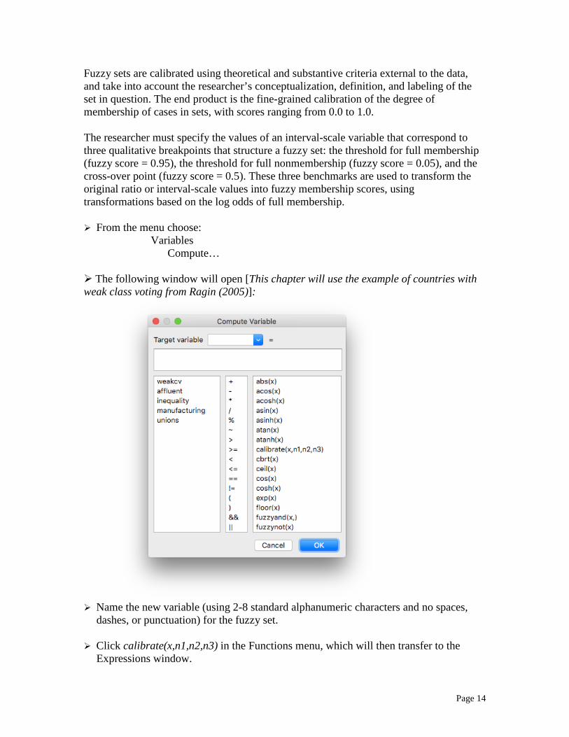
Fuzzy sets are calibrated using theoretical and substantive criteria external to the data, and take into account the researcher’s conceptualization, definition, and labeling of the set in question. The end product is the fine-grained calibration of the degree of membership of cases in sets, with scores ranging from 0.0 to 1.0. The researcher must specify the values of an interval-scale variable that correspond to three qualitative breakpoints that structure a fuzzy set: the threshold for full membership (fuzzy score = 0.95), the threshold for full nonmembership (fuzzy score = 0.05), and the cross-over point (fuzzy score = 0.5). These three benchmarks are used to transform the original ratio or interval-scale values into fuzzy membership scores, using transformations based on the log odds of full membership. From the menu choose:

Variables Compute… The following window will open [This chapter will use the example of countries with weak class voting from Ragin (2005)]:

Name the new variable (using 2-8 standard alphanumeric characters and no spaces,

dashes, or punctuation) for the fuzzy set. Click calibrate(x,n1,n2,n3) in the Functions menu, which will then transfer to the

Expressions window.

Page 15

Edit the expression calibrate(,,,), for example, “calibrate(manf,25,10,2).” Here, manf

is the name of an existing interval or ratio scale variable already in the file, which you can transfer from the Variables menu on the left. The first number is the value of oldvar that corresponds to the threshold for full membership in the target set (0.95), the second number is value of oldvar that corresponds to the cross-over point (0.5) in the target set, and the third number is the value of oldvar that corresponds to the threshold for nonmembership in the target set (0.05).

Click “OK.” Check the data spreadsheet to make sure the fuzzy scores correspond to the original

values in the manner intended. It may be useful to sort the variable in descending or ascending order, by clicking on the variable name in the column heading. The result is a fine-grained calibration of the degree of membership of cases in sets, with scores ranging from 0 to 1.

Add / Insert Cases In order to add cases into an already existing data sheet, choose: Cases Add… The following window will appear:

Enter the number of cases you want to add to the existing number of cases. The

additional case(s) will appear at the end (bottom) of the data spreadsheet. Delete Cases In order to delete single cases from an already existing data sheet, highlight the case

that you want to delete and choose: Cases Delete…

Page 16

The following window will appear:

With this function you can only delete one case at a time. The program will ask you whether you want to delete the case in which you have

highlighted a cell in the data sheet. Select Cases If Select Cases If provides several methods for selecting a subgroup of cases based on criteria that include variables and complex expressions, like: - Variable values and ranges - Arithmetic expressions - Logical expressions - Functions Unselected cases remain in the data file but are excluded from analysis. Unselected cases are indicated by a faded appearance in the data spreadsheet. In order to select a subset of cases for analysis, choose: Cases Select If… The following window will open:

Page 17

Specify the criteria for selecting cases. If the result of a conditional expression is true, the case is selected. If the result of a

conditional expression is false or missing, the case is not selected. Most conditional expressions use one or more of the six relational operators (<, >,

<=, >=, ==, !=) on the calculator pad. Conditional expressions can include variable names, constants, arithmetic operators,

numeric and other functions, logical variables, and relational operators. Note: “Select If” works best when it is univariate. For example, if you want to use the

“Select If” function combining two logical statements, e.g., both a logical AND and a logical NOT, try creating a new variable (with compute or recode) that reflects your selection criteria and then use the new variable with “Select If.”

If you want to reverse your selection, choose: Cases Cancel Selection… C) Working with Output When you run a procedure, the results are displayed in the fsQCA window. You can use scroll up and down the window to browse the results.

Page 18

In order to print output, choose: File Print Results… Your computer specific printer options window will appear, in which you can specify

your printing options. The output is written in monospace New Courier (10) in order allow simple transport

between programs. Therefore, if you open the *.out file in SPSS or some other program, the numbers in the tables will be slightly dislocated, unless you specify the appropriate font.

Output may also be copied and pasted into Word, Wordpad, Text, or other files. In order to save results, choose: File

Save Results... fsQCA will save results in *.txt (plain text) format. Chapter 3. BASIC STATISTICS AND GRAPHS [This chapter will use the example of countries with weak class voting from Ragin (2005).] Necessary Conditions The Necessary Conditions procedure produces consistency and coverage scores for individual conditions and/or specified substitutable conditions. In order to analyze necessary conditions, choose: Analyze Necessary Conditions…

Page 19

The following window will open…

Select the outcome in the drop-down Outcome menu. Then select a condition from

the drop-down Add Conditions menu and then transfer it to the Conditions box on the right-hand side of the Dialog window. You can specify substitutable necessary conditions using logical or (+).

Once you’ve entered the specifications, click OK and the analysis will be displayed.

Page 20

In this context, consistency indicates the degree to which the causal condition is a superset of the outcome; coverage indicates the empirical relevance of a consistent superset. Set Coincidence The Set Coincidence procedure assesses the degree of overlap of two or more sets. In order to analyze the coincidence of two or more sets, choose: Analyze Set Coincidence… The following window will open…

Page 21

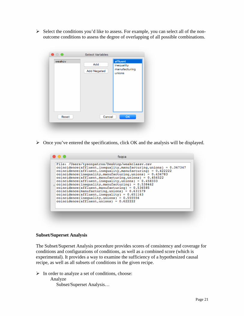
Select the conditions you’d like to assess. For example, you can select all of the non-outcome conditions to assess the degree of overlapping of all possible combinations.

Once you’ve entered the specifications, click OK and the analysis will be displayed.

Subset/Superset Analysis The Subset/Superset Analysis procedure provides scores of consistency and coverage for conditions and configurations of conditions, as well as a combined score (which is experimental). It provides a way to examine the sufficiency of a hypothesized causal recipe, as well as all subsets of conditions in the given recipe. In order to analyze a set of conditions, choose: Analyze Subset/Superset Analysis…

Page 22

The following window will open:

Select the outcome variable and click Set. Then choose the causal conditions and

click Add or Add Negated, depending on your expectations.

Once you’ve entered the specifications, click OK and the following window will

open:

Page 23

Once you’ve run the analysis, you can choose to save the results to a file in *.csv

format, or send the result to the output window. The following shows the results in the output window

Descriptives The Descriptives procedure displays univariate summary statistics for specified conditions in a single table. In order to obtain descriptive statistics, choose: Analyze Statistics

Page 24

Descriptives… Select one or more conditions from the Variables column and transfer them into the

Descriptives column. Click Ok. The output window will show your descriptive statistics:

The first line of your output will state the file name and the procedure you have chosen

(Descriptive Statistics). The columns in the descriptives table indicate the following:

1. The variable chosen (Variable) 2. The mean value (Mean) 3. The standard deviation (Std. Dev.) 4. The lowest value of the variable (Minimum) 5. The highest value of the variable (Maximum) 6. The number of cases (N Cases) 7. The number of missing cases (Missing)

Graphs XY Plot In order to produce a XY Plot, choose: Graphs XY Plot... The following window will open:

Page 25

Select a variable to define the values on the X Axis shown in the chart. Select a variable to define the values on the Y Axis shown in the chart. You can also add more information by choosing a Case ID Variable. This variable

will not be represented in the graph, but you can determine its value by moving the cursor to a particular point in the graph after you’ve plotted the graph. For example, the Case ID variable could be a string variable with the names of the countries in the data set. Once plotted, it is possible to move the cursor to any point in the plot, and a window will appear with the case name and the x and y values of the point.

Once you have entered the specifications, click the Plot button and the plot will be

displayed:

Page 26

The numbers below the “Plot” button show set-theoretic consistency scores. The upper

line shows the degree to which the data plotted are consistent with X ≤ Y (X is a subset of Y). The lower line shows the degree to which the data plotted are consistent with X ≥ Y (Y is a subset of X). If one of these two numbers indicates high consistency, the other can be interpreted as a coverage score. For example, if the number in the upper line is .91 and the number in the lower line is .63, these calculations indicate that the data are largely consistent with the argument that X is a subset of Y and its coverage of Y is 63%. That is, X accounts for 63% of the sum of the memberships in Y.

You can negate variables in the graph by clicking on the negate option next to the

variable name. This feature will subtract the fuzzy-set value of this variable from 1. Example: Inequality = .4; negation of Inequality = .6. [Same as ‘~’ and ‘fuzzynot(x)’]

You can copy the graph as an image and paste it into Word, Text, or other files.

Page 27

4. CRISP-SET ANALYSIS This part of the manual refers to the analysis of dichotomous social data reflecting the memberships of cases in conventional, crisp sets. In-depth discussions of this method can be found in The Comparative Method (Ragin 1987), in chapter 5 of Fuzzy-Set Social Science (Ragin 2000). The data analytic strategy used here is known as qualitative comparative analysis, or QCA. QCA is based on Boolean algebra, where a case is either in or out of a set, and QCA uses binary-coded data, with 1 indicating membership and 0 indicating nonmembership. QCA using conventional, crisp sets is also known as csQCA. A) Basic Concepts

An explicit algebraic basis for qualitative comparison exists in Boolean algebra. Also known as the algebra of logic and as the algebra of sets, Boolean algebra was developed in the mid-nineteenth century by George Boole. The Boolean principles used in qualitative comparative analysis are quite simple. Seven aspects of Boolean algebra are essential for the algorithms and are presented here in rough sequence, with more difficult concepts following simpler concepts. 1) Use of binary data There are two conditions or states in Boolean algebra: true (or present) and false (or absent). These two states are represented in base 2: 1 indicates presence; 0 indicates absence. The typical Boolean-based comparative analysis addresses the presence/absence of conditions under which a certain outcome is obtained (that is, is true). Thus, in a Boolean analysis of social data all variables, causal conditions and outcome, must be nominal-scale measures, preferably binary. Interval-scale measures are transformed into multi-category nominal-scale measures. Nominal-scale measures with more than two categories are represented with several binary variables. 2) Boolean negation In Boolean logic, negation switches membership scores from 1 to 0 and from 0 to 1. The negation of the crisp set of males, for example, is the crisp set of not males. If a case has a Boolean score of 1 in the set of males, then it has a Boolean score of 0 in the set of not males. 3) Use of truth table to represent data In order to use Boolean algebra as a technique of qualitative comparison, it is necessary to reconstruct a raw data matrix as a truth table. The idea behind a truth table is simple. Once the data have been recoded into nominal-scale variables and represented in binary form (as 1's and 0's), it is necessary only to sort the data into their different combinations of values on the casual conditions. Each logical combination of values on the causal conditions is represented as one row of the truth table. Once this part of the truth table is constructed, each row is assigned an output value (a score of 1 or 0 on the outcome) based on the scores of the cases which share that combination of input values (that

Page 28

combination of scores on the causal conditions). Thus, both the different combinations of input values (causal conditions) and their associated output values (the outcome) are summarized in a truth table. Truth tables have as many rows as there are logically possible combinations of values on the causal conditions. If there are three binary causal conditions, for example, the truth table will contain 23 = 8 rows, one for each logically possible combination of three presence/absence conditions. The truth table for a moderate-sized data set with three binary conditions and one binary outcome (with 1 = present and 0 = absent) is shown in Table 1. Technically, there is no reason to include the frequency of each combination as part of the truth table. These values are included in the examples to remind the reader that each row is not a single case but a summary of all the cases with a certain combination of input values. In this respect, a row of a truth table is like a cell from a multiway cross-classification of several categorical independent variables. Table 1: Hypothetical Truth Table Showing Three Causes of Regime Failure Condition Regime Failure Number

of Instances

conflict death cia failure

0 1 0 0 1 1 0 1

0 0 1 0 1 0 1 1

0 0 0 1 0 1 1 1

0 1 1 1 1 1 1 1

9 2 3 1 2 1 1 3

conflict = Conflict between older and younger military officers death = Death of a powerful dictator cia = CIA dissatisfaction with the regime 4) Groupings Just as it is possible to calculate the logically possible number of combinations (2k), it is also possible to calculate the number of logically possible groupings. The formula is 3k-1, where k again is the number of attributes (33 -1 = 26). Table 2 shows the 26 logically possible groupings of the three dichotomies presented in Table 1. Using the formula just described, the 26 possible groupings are formed as follows: 8 involve combinations of three attributes, 12 involve combinations of two attributes, and six involve single attributes. Table 2: Groupings Using Three Dichotomies (from Table 1)

Page 29

Initial Configuration (8 combinations of three

aspects)

Groupings involving combinations of two aspects

(12)

Groupings evolving a single aspect (6)

conflict • death • cia conflict • death • ~cia conflict • ~death • cia

conflict • ~death • ~cia ~conflict • death • cia

~conflict • ~death • cia conflict • death • ~cia

~conflict • ~death • ~cia

conflict • death conflict • ~death

~conflict • ~death ~conflict • death

conflict • cia conflict • ~cia ~conflict • cia

~conflict • ~cia death • cia

death • ~cia ~death • cia

~death • ~cia

conflict ~conflict

death ~death

cia ~cia

5) Boolean Addition In Boolean algebra, if A + B = Z, and A = 1 and B = 1, then Z = 1. In other words, 1 + 1 = 1. The basic idea in Boolean addition is that if any of the additive terms is satisfied (present), then the outcome is true (occurs). Addition in Boolean algebra is equivalent to the logical operator OR. (In this discussion uppercase OR is used to indicate logical OR.) Thus, the above statement A + B = Z becomes: if A equals 1 OR B equals 1, then Z equals 1. The best way to think of this principle is in logical terms, not arithmetically. For example, there might be several things a person could do to lose his or her job. It does not matter how many of these things the person does. If the employee does any one (or all) of them, he or she will be fired. Doing two of them will not cause one employee to be more fired than another employee who does only one of them. Fired is fired, a truly qualitative state. This example succinctly illustrates the nature of Boolean addition: satisfy any one of the additive conditions and the expected outcome follows. Consider the collapse of military regimes. Assume that there are three general conditions that cause military regimes to fall: sharp conflict between older and younger military officers (conflict), death of a powerful dictator (death), or CIA dissatisfaction with the regime (cia). Any one of these three conditions may be sufficient to prompt a collapse. The truth table for a number of such regimes in different countries is shown in Table 1 (with 1 = present and 0 = absent). Each combination of causes produces either regime failure or an absence of regime failure – there are no contradictory rows.

The "simplified" Boolean equation

failure = conflict + death + cia

Page 30

expresses the relation between the three conditions and regime failure simply and elegantly for both negative and positive instances. Simply stated: if any one (or any two or all three) of these conditions obtains, then the regime will fall. 6) Boolean Multiplication Boolean multiplication differs substantially from normal multiplication. Boolean multiplication is relevant because the typical social science application of Boolean algebra concerns the process of simplifying expressions known as "sums of products." A product is a particular combination of causal conditions. The data on collapsed military regimes from Table 1 can be represented in "primitive" (that is, unreduced) sums-of-products form as follows:

failure = conflict • ~death • ~cia + ~conflict • death • ~cia + ~conflict • ~death • cia + conflict • death • ~cia + conflict • ~death • cia + ~conflict • death • cia + conflict • death • cia

Each of the seven terms represents a combination of causal conditions found in at least one instance of regime failure. The different terms are products because they represent intersections of conditions (conjunctures of causes and absences of causes). The equation shows the different primitive combinations of conditions that are linked to the collapse of military regimes. Boolean multiplication, like Boolean addition, is not arithmetic. The expression conflict • ~death • ~cia does not mean that the value of conflict (1) is multiplied by the value of death (0) and by the value of cia (0) to produce a result value of 0. It means simply that a presence of conflict is combined with an absence of death and an absence of cia. The total situation, failure = conflict • ~death • ~cia, occurs in the data twice. This conjunctural character of Boolean multiplication shapes the interpretation of the primitive sums-of-products equation presented above: failure (regime failure) occurs if any of seven combinations of three causes is obtained. In Boolean algebra addition indicates logical OR and multiplication indicates logical AND. The three causes are ANDed together in different ways to indicate different empirical configurations. These intersections are ORed together to form an unreduced, sums-of-products equation describing the different combinations of the three causes linked to regime collapse. 7) Combinatorial Logic Boolean analysis is combinatorial by design. In the analysis of regime failures presented above, it appears from casual inspection of only the first four rows of the truth table (Table 1) that if any one of the three causes is present, then the regime will collapse. While it is tempting to take this shortcut, the route taken by Boolean analysis is much

Page 31

more exacting of the data. This is because the absence of a cause has the same logical status as the presence of a cause in Boolean analysis. As noted above, Boolean multiplication indicates that presence and absence conditions are combined, that they intersect. Consider the second row of the truth table (Table 1), which describes the two instances of military regime failure linked to causal configuration conflict • ~death • ~cia. Simple inspection suggests that in this case failure (regime failure) resulted from the first cause, conflict. But notice that if the investigator had information on only this row of the truth table, and not on any of the other instances of regime failure, he or she might conclude that conflict causes failure only if causes death and cia are absent. This is what the conflict • ~death • ~cia combination indicates. This row by itself does not indicate whether conflict would cause failure in the presence of death or cia or both. All the researcher knows from these two instances of conflict • ~death • ~cia is that for conflict to cause failure, it may be necessary for the other conditions (death and cia) to be absent. From a Boolean perspective, it is entirely plausible that in the presence of one or both of these other conditions (say, configuration conflict • ~death • cia), failure may not result. To return to the original designations, it may be that in the presence of CIA meddling (cia), conflict between junior and senior officers (conflict) will dissipate as the two factions unite to oppose the attempt by outsiders to dictate events. To push this argument further, assume the investigator had knowledge of only the first four rows of the truth table. The data would support the idea that the presence of any one of the three conditions causes failure, but again the data might indicate that conflict causes failure only when death and cia are absent (conflict • ~death • ~cia); death causes failure only when conflict and cia are absent (~conflict • death • ~cia), and so on. A strict application of combinatorial logic requires that these limitations be placed on conclusions drawn from a limited variety of cases. This feature of combinatorial logic is consistent with the idea that cases, especially their causally relevant features, should be viewed holistically. The holistic character of the Boolean approach is consistent with the orientation of qualitative scholars in comparative social science who examine different causes in context. When the second row of the truth table (Table 1) is examined, it is not interpreted as instances of failure caused by conflict, but as instances of failure caused by conflict • ~death • ~cia. Thus, in Boolean-based qualitative comparison, causes are not viewed in isolation but always within the context of the presence and absence of other causally relevant conditions. Minimization The restrictive character of combinatorial logic seems to indicate that the Boolean approach simply compounds complexity on top of complexity. This is not the case. There are simple and straightforward rules for simplifying complexity – for reducing primitive expressions and formulating more succinct Boolean statements. The most fundamental of these rules is:

Page 32

If two Boolean expressions differ in only one causal condition yet produce the same outcome, then the causal condition that distinguishes the two expressions can be considered irrelevant and can be removed to create a simpler, combined expression. Essentially this minimization rule allows the investigator to take two Boolean expressions that differ in only one term and produce a combined expression. For example, conflict • ~death • ~cia and conflict • death • ~cia, which both produce outcome failure, differ only in death; all other elements are identical. The minimization rule stated above allows the replacement of these two terms with a single, simpler expression: conflict • ~cia. In other words, the comparison of these two rows, conflict • ~death • ~cia and conflict • death • ~cia, as wholes indicates that in instances of conflict • ~cia, the value of death is irrelevant. The condition death may be either present or absent; failure will still occur. The logic of this simple data reduction parallels the logic of experimental design. Only one causal condition, death, varies and no difference in outcome is detected (because both conflict • ~death • ~cia and conflict • death • ~cia are instances of failure). According to the logic of experimental design, death is irrelevant to failure in the presence of conflict • ~cia (that is, holding these two conditions constant). Thus, the process of Boolean minimization mimics the logic of experimental design. It is a straightforward operationalization of the logic of the ideal social scientific comparison. This process of logical minimization is conducted in a bottom-up fashion until no further stepwise reduction of Boolean expressions is possible. Consider again the data on military regime failures presented above. Each of the rows with one cause present and two absent can be combined with rows with two causes present and one absent because all these rows have the same outcome (failure) and each pair differs in only one causal condition: conflict • ~death • ~cia combines with conflict • death • ~cia to produce conflict • ~cia. conflict • ~death • ~cia combines with conflict • ~death • cia to produce conflict • ~death. ~conflict • death • ~cia combines with conflict • death • ~cia to produce death • ~cia. ~conflict • death • ~cia combines with ~conflict • death • cia to produce ~conflict • death. ~conflict • ~death • cia combines with conflict • ~death • cia to produce ~death • cia. ~conflict • ~death • cia combines with ~conflict • death • cia to produce ~conflict • cia. Similarly, each of the rows with two causes present and one absent can be combined with the row with all three present: conflict • death • ~cia combines with conflict • death • cia to produce conflict • death. conflict • ~death • cia combines with conflict • death • cia to produce conflict • cia. ~conflict • death • cia combines with conflict • death • cia to produce death • cia. Further reduction is possible. Note that the reduced terms produced in the first round can be combined with the reduced terms produced in the second round to produce even simpler expressions:

Page 33

conflict • ~death combines with conflict • death to produce conflict. conflict • ~cia combines with conflict • cia to produce conflict. ~conflict • death combines with conflict • death to produce death. death • ~cia combines with death • cia to produce death. ~conflict • cia combines with conflict • cia to produce cia. ~death • cia combines with death • cia to produce cia. Although tedious, this simple process of minimization produces the final, reduced Boolean equation: failure = conflict + death + cia True enough, this was obvious from simple inspection of the entire truth table, but the problem presented was chosen for its simplicity. The example directly illustrates key features of Boolean minimization. It is bottom-up. It seeks to identify ever wider sets of conditions (that is, simpler combinations of causal conditions) for which an outcome is true. And it is experiment-like in its focus on pairs of configurations differing in only one cause. 1) Use of “prime implicants” A further Boolean concept that needs to be introduced is the concept of implication. A Boolean expression is said to imply another if the membership of the second term is a subset of the membership of the first. For example, a implies a • ~b • ~c because a embraces all the members of a • ~b • ~c (that is, a • ~b • ~c is a subset of a). This concept is best understood by example. If a indicates economically dependent countries, b indicates the presence of heavy industry, and c indicates centrally coordinated economies, a embraces all dependent countries while a • ~b • ~c embraces all dependent countries that lack both centrally coordinated economies and heavy industry. Clearly the membership of a • ~b • ~c is included in the membership of a. Thus, a implies a • ~b • ~c. The concept of implication, while obvious, provides an important tool for minimizing primitive sums-of-products expressions. Consider the hypothetical truth table shown in Table 3, which summarizes data on three causal conditions thought to affect the success of strikes already in progress (success): a booming market for the product produced by the strikers (market), the threat of sympathy strikes by workers in associated industries (threat), and the existence of a large strike fund (fund). The Boolean equation for success (successful strikes) showing unreduced (primitive) Boolean expressions is success = market • ~threat • fund + ~market • threat • ~fund +

market • threat • ~fund + market • threat • fund

Page 34

Table 3: Hypothetical Truth Table Showing Three Causes of Successful Strikes

Condition Success Frequency Market Threat fund success

1 0 1 1 1 0 0 0

0 1 1 1 0 0 1 0

1 0 0 1 0 1 1 0

1 1 1 1 0 0 0 0

6 5 2 3 9 6 3 4

The first step in the Boolean analysis of these data is to attempt to combine as many compatible rows of the truth table as possible. (Note that this part of the minimization process uses rows with an output value of 1, strike succeeded.) This first phase of the minimization of the truth table produces the following partially minimized Boolean equation, which in effect turns a primitive Boolean equation with four three-variable terms into an equation with three two-variable terms: market • threat • fund combines with market • ~threat • fund to produce market • fund. market • threat • fund combines with market • threat • ~fund to produce market • threat. market • threat • ~fund combines with ~market • threat • ~fund to produce threat • ~fund.

success = market • fund + market • threat + threat • ~fund

Product terms such as those in the preceding equation which are produced using this simple minimization rule—combine rows that differ on only one cause if they have the same output values—are called prime implicants. Usually, each prime implicant covers (that is, implies) several primitive expressions (rows) in the truth table. In the partially minimized equation given above, for example, prime implicant market • fund covers two primitive Boolean expressions listed in the truth table: market • threat • fund and market • ~threat • fund. This partially reduced Boolean expression illustrates a common finding in Boolean analysis: often there are more reduced expressions (prime implicants) than are needed to cover all the original primitive expressions. Prime implicant market • threat implies primitive terms market • threat • fund and market • threat • ~fund, for example, yet these two primitive terms are also covered by market • fund and threat • ~fund, respectively. Thus, market • threat may be redundant from a purely logical point of view; it may not be an essential prime implicant. In order to determine which prime implicants are logically essential, a minimization device known as a prime implicant chart is used. Minimization of the prime implicant chart is the second phase of Boolean minimization.

Page 35

Briefly stated, the goal of this second phase of the minimization process is to "cover" as many of the primitive Boolean expressions as possible with a logically minimal number of prime implicants. This objective derives from a straightforward desire for non-redundancy. The prime implicant chart maps the links between prime implicants and primitive expressions. The prime implicant chart describing these links in the data on strike outcomes is presented in Table 4. Simple inspection indicates that the smallest number of prime implicants needed to cover all of the original primitive expressions is two. (For very complex prime implicant charts, sophisticated computer algorithms are needed; see Mendelson 1970, Roth 1975, and McDermott 1985.) Prime implicants market • fund and threat • ~fund cover all four primitive Boolean expressions. Analysis of the prime implicant chart, therefore, leads to the final reduced Boolean expression containing only the logically essential prime implicants:

success = market • fund + threat • ~fund

This equation states simply that successful strikes occur when there is a booming market for the product produced by the workers AND a large strike fund (market • fund) or when there is the threat of sympathy strikes by workers in associated industries combined with a low strike fund (threat • ~fund). (Perhaps the threat of sympathy strikes is taken seriously only when the striking workers badly need the support of other workers.) Table 4: Prime Implicant Chart Showing Coverage of Original Terms by Prime Implicants (Hypothetical Strike Data)

Primitive Expressions

market • threat •

fund

market • ~threat •

fund

market • threat • ~fund

~market • threat • ~fund

Prime Implicants

market • fund X X market • threat X X threat • ~fund X X

These simple procedures allow the investigator to derive a logically minimal equation describing the different combinations of conditions associated with an outcome. The final, reduced equation shows the two (logically minimal) combinations of conditions that cause successful strikes and thus provides an explicit statement of multiple conjunctural causation. 2) Use of De Morgan's Law The application of De Morgan's Law is straightforward. Consider the solution to the hypothetical analysis of successful strikes presented above: success = market • fund + threat • ~fund. Elements that are coded present in the reduced equation (say, market in the term market • fund) are recoded to absent, and elements that are coded absent (say,

Page 36

~fund in the term threat • ~fund) are recoded to present. Next, logical AND is recoded to logical OR, and logical OR is recoded to logical AND. Applying these two rules, success = market • fund + threat • ~fund becomes: ~success = (~market + ~fund)• (~threat + fund)

= ~market • ~threat + ~market • fund + ~threat • ~fund

According to this equation, strikes fail when (1) the market for the relevant product is not booming AND there is no serious threat of sympathy strikes, (2) the market for a product is not booming AND there is a large strike fund, OR (3) there is no threat of sympathy strikes AND only a small strike fund. (The combination ~market • fund—nonbooming market and large strike fund, which seems contradictory—may suggest an economic downturn after a period of stability. In this situation a shutdown might be welcomed by management.) De Morgan’s Law produces the exact negation of a given logical equation. If there are “remainder” combinations in the truth table and they are used as “don’t cares,” then the results of the application of De Morgan Law will yield a logical statement that is not the same as the analysis of the absence of the outcome. Likewise, if the remainders are defined as “false” in the initial analysis, then the application of De Morgan’s Law to the solution (of positive cases) will yield a logical statement that embraces not only the negative cases, but also the remainders. 3) Necessary and Sufficient Causes A cause is defined as necessary if it must be present for an outcome to occur. A cause is defined as sufficient if by itself it can produce a certain outcome. This distinction is meaningful only in the context of theoretical perspectives. No cause is necessary, for example, independent of a theory that specifies it as a relevant cause. Neither necessity nor sufficiency exists independently of theories that propose causes. Necessity and sufficiency are usually considered together because all combinations of the two are meaningful. A cause is both necessary and sufficient if it is the only cause that produces an outcome and it is singular (that is, not a combination of causes). A cause is sufficient but not necessary if it is capable of producing the outcome but is not the only cause with this capability. A cause is necessary but not sufficient if it is capable of producing an outcome in combination with other causes and appears in all such combinations. Finally, a cause is neither necessary nor sufficient if it appears only in a subset of the combinations of conditions that produce an outcome. In all, there are four categories of causes (formed from the cross-tabulation of the presence/absence of sufficiency against the presence/absence of necessity).

Page 37

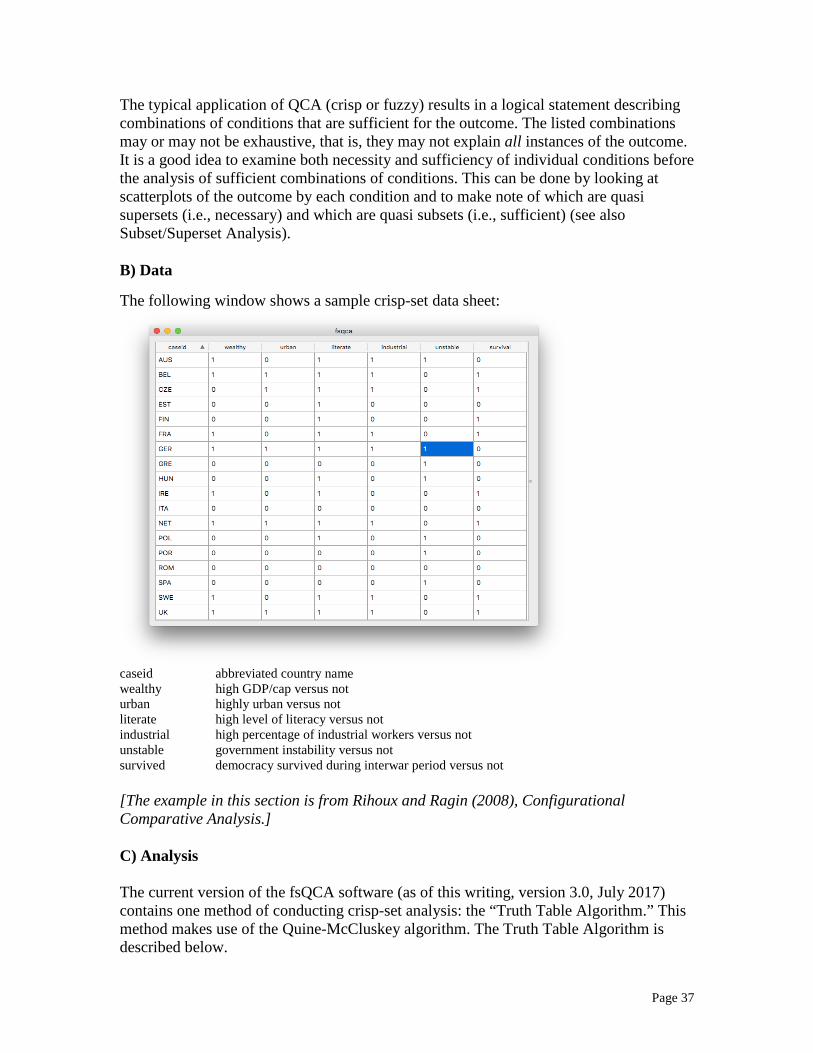
The typical application of QCA (crisp or fuzzy) results in a logical statement describing combinations of conditions that are sufficient for the outcome. The listed combinations may or may not be exhaustive, that is, they may not explain all instances of the outcome. It is a good idea to examine both necessity and sufficiency of individual conditions before the analysis of sufficient combinations of conditions. This can be done by looking at scatterplots of the outcome by each condition and to make note of which are quasi supersets (i.e., necessary) and which are quasi subsets (i.e., sufficient) (see also Subset/Superset Analysis). B) Data The following window shows a sample crisp-set data sheet:

caseid abbreviated country name wealthy high GDP/cap versus not urban highly urban versus not literate high level of literacy versus not industrial high percentage of industrial workers versus not unstable government instability versus not survived democracy survived during interwar period versus not [The example in this section is from Rihoux and Ragin (2008), Configurational Comparative Analysis.] C) Analysis The current version of the fsQCA software (as of this writing, version 3.0, July 2017) contains one method of conducting crisp-set analysis: the “Truth Table Algorithm.” This method makes use of the Quine-McCluskey algorithm. The Truth Table Algorithm is described below.

Page 38

Truth Table Algorithm Two important tasks structure the application of the crisp-set truth table algorithm: (1) The assessment of the distribution of cases across different logically possible combinations of causal conditions. And (2) the assessment of the consistency of the evidence for each causal combination with the argument that the cases with this combination of conditions constitute a subset of the cases with the outcome. That is, they share the outcome in question The truth table algorithm involves a two-step analytic procedure. The first step consists of creating a truth table spreadsheet from the raw data, which primarily involves specifying the outcome and causal conditions to include in the analysis. The second step consists of preparing the truth table spreadsheet for analysis, by selecting both a frequency threshold and a consistency threshold. In order to create the truth table spreadsheet, choose: Analyze Truth Table Algorithm… The following window will open, listing the variables in your file:

Identify and highlight the case aspect you want to explain and transfer it into the

Outcome field by clicking Set. Select a preliminary list of causal conditions by highlighting one at a time and clicking

Add to move them over one by one to the Causal Conditions field. Check the box next to “Show solution cases in output” and choose the variable that is

your caseID.

Page 39

Click on the Okay button and the following window containing the full truth table will appear:

The truth table will have 2k rows (where k represents the number of causal conditions),

reflecting all possible combinations of causal conditions (scroll down to see all possible combinations). The 1s and 0s represent full membership and zero membership for each condition, respectively. For each row, a value for each of the following variables is created:

number the number of cases displaying the combination of conditions raw consist. the proportion of cases in each truth table row that display the outcome. PRI consist. an alternative measure of consistency (developed for fuzzy sets) based on

a quasi proportional reduction in error calculation. In crisp set analyses this will be equal to raw consist.

SYM consist. an alternative measure of consistency for fuzzy sets based on a symmetrical version of PRI consistency.

Note that the column labeled as the outcome (survived in this example) is blank. It is up to the investigator to determine the outcome for each configuration using the following procedure. The researcher must begin by developing a rule for classifying some combinations

(rows) as relevant and others as irrelevant, based on their frequency. This is accomplished by selecting a frequency threshold based on the number of cases in each row, shown in the number column. When the total number of cases in an analysis is relatively small, the frequency threshold should be 1 or 2. When the total N is large,

Page 40

however, a more substantial threshold should be used. It is very important to examine the distribution of cases across causal combinations.

Configurations (rows) can be sorted by their frequency (descending or ascending) by

clicking the heading of the number column. After sorting rows and selecting a frequency threshold, delete all rows that do not meet

the threshold. If the cases have been sorted in a descending order according to number, click on the first case that falls below the threshold then select

Edit Delete current row to last row… If cases have not been sorted then those cases that do not meet the threshold can be deleted individually by selecting the row the choosing Edit Delete current row… The next step is to distinguish configurations that are subsets of the outcome from

those that are not. For crisp sets, this determination is made using the measure of set-theoretic consistency reported in the raw consist column. Values below 0.75 indicate substantial inconsistency. It is useful to sort the consistency scores in descending order to evaluate their distribution (this should be done after removing rows that fail to meet the frequency threshold). Sorting is accomplished by clicking the raw consist. column label.

Identify any gaps in the upper range of consistency that might be useful for

establishing a consistency threshold. Keep in mind that it is always possible to examine several different thresholds and assess the consequences of lowering and raising the consistency cut-off.

It is now necessary to indicate which configurations can be considered subsets of the

outcome and which cannot (see also alternative method below). Input a 1 in the outcome column (survived in this example) for each configuration whose consistency level meets and/or exceeds the threshold. Input a 0 in the outcome column for each configuration whose consistency level does not meet the consistency threshold.

Alternatively, one can use the “Delete and code” function to automate this process.

Select: Edit Delete and code… In the first field, the frequency threshold is selected. The default number of cases is 1, but may be changed by typing the selected frequency threshold into the field. In the second field, the consistency threshold is selected. The default consistency is 0.8, but this may be changed by typing the selected consistency threshold into the field.

Page 41

Click “OK.” The program will delete rows where the frequency threshold is not met, and will code the outcome as 0 or 1 depending on the selected consistency threshold. The following window displays the truth table that would appear after

1. applying a frequency threshold of 1 to the data and eliminating configurations that do not have any observations (6 configurations)

2. selecting a consistency threshold of 0.9 and placing a 1 in the survived column for configurations with 0.90 consistency or greater (4 configurations) and a 0 for cases with lower consistency (6 configurations)

From here, there are two possibilities for the analysis: specifying a single analysis versus deriving the three “standard” analyses (complex, parsimonious, and intermediate). Clicking the “Standard Analyses” button (which gives the three solutions) is the recommended procedure. i) Specify Analysis Option Once the truth table is constructed (before clicking “Standard Analyses”) select

Specify Analysis to bring up the Truth Table Analysis Window. In the Specify panel setting Positive cases to “True” and all the others to “False” will

yield the “most complex” solution. This window appears as:

Page 42

To derive the most parsimonious solution, set Positive cases to “True,” Negative Cases

to “False”, and Remainders to “Don’t Cares.” Please note: When the algorithm for selecting prime implicants cannot fully reduce the

truth table, the Prime Implicant Window will appear and the user must select the prime implicants to be used, based on theoretical and substantive knowledge. This window is most likely to pop open when the program is deriving the parsimonious solution, but could happen for all three solutions. (See below in Fuzzy-Set Analysis for a description of how this window operates.)

To perform the analysis, click the Okay button and the output will appear in the output

window. ii) Standard Analyses Option Once the truth table is fully constructed, select Standard Analyses. Standard Analyses

automatically provides the user with the complex, parsimonious, and intermediate solutions. “Standard Analyses” is the recommended procedure, as this is the only way to derive the intermediate solution. To derive the intermediate solution, the software conducts counterfactual analyses based on information about causal conditions supplied by the user.

Limited Diversity and Counterfactual Analysis One of the most challenging aspects of comparative research is the simple fact that researchers work with relatively small Ns. Investigators often confront "more variables than cases," a situation that is greatly complicated the fact that comparativists typically focus on combinations of case aspects – how aspects of cases fit together configurationally. For example, a researcher interested in a causal argument specifying an intersection of four causal conditions ideally should consider all sixteen logically possible combinations of these

Page 43

four conditions in order to provide a thorough assessment of this argument. Naturally occurring social phenomena, however, are profoundly limited in their diversity. The empirical world almost never presents social scientists all the logically possible combinations of causal conditions relevant to their arguments (as shown with hypothetical data in Table 1 below). While limited diversity is central to the constitution of social and political phenomena, it also severely complicates their analysis. Table 1: Truth table with four causal conditions (A, B, C, and D) and one outcome (Y)

A B C D Y* no no no no no no no no yes ? no no yes no ? no no yes yes ? no yes no no no no yes no yes no no yes yes no ? no yes yes yes no yes no no no ? yes no no yes ? yes no yes no ? yes no yes yes ? yes yes no no yes yes yes no yes yes yes yes yes no ? yes yes yes yes ?

* Rows with "?" in the Y column lack cases – the outcome cannot be determined. As a substitute for absent combinations of causal conditions, comparative researchers often engage in "thought experiments" (Weber [1905] 1949). That is, they imagine counterfactual cases and hypothesize their outcomes, using their theoretical and substantive knowledge to guide their assessments. Because QCA uses truth tables to assess cross-case patterns, this process of considering counterfactual cases (i.e., absent combinations of causal conditions) is explicit and systematic. In fact, this feature of QCA is one of its key strengths. However, the explicit consideration of counterfactual cases and the systematic incorporation of the results of such assessments into statements about cross-case patterns are relatively new to social science. The specification of best practices with respect to QCA and counterfactual analysis, therefore, is essential. Consider an example (not based on Table 1 above). A researcher postulates, based on existing theory, that causal conditions A, B, C, and D are all linked in some way to outcome Y. That is, it is the presence of these conditions, not their absence, which should be linked to the presence of the outcome. The empirical evidence indicates that many instances of Y are coupled with the presence of causal conditions A, B, and C, along with the absence of condition D (i.e., A⋅B⋅C⋅d Y). The researcher suspects, however, that all that really matters is having the first three causes, A, B and C. In order for A⋅B⋅C to generate Y, it is

Page 44

not necessary for D to be absent. However, there are no observed instances of A, B, and C combined with the presence of D (i.e., no observed instances of A⋅B⋅C⋅D). Thus, the decisive empirical case for determining whether the absence of D is an essential part of the causal mix (with A⋅B⋅C) simply does not exist. Through counterfactual analysis (i.e., a thought experiment), the researcher could declare this hypothetical combination (A⋅B⋅C⋅D) to be a likely instance of the outcome (Y). That is, the researcher might assert that A⋅B⋅C⋅D, if it existed, would lead to Y. This counterfactual analysis would allow the following logical simplification: A⋅B⋅C⋅d + A⋅B⋅C⋅D Y A⋅B⋅C⋅(d + D) Y A⋅B⋅C Y How plausible is this simplification? The answer to this question depends on the state of the relevant theoretical and substantive knowledge concerning the connection between D and Y in the presence of the other three causal conditions (A⋅B⋅C). If the researcher can establish, on the basis of existing knowledge, that there is every reason to expect that the presence of D should contribute to outcome Y under these conditions (or conversely, that the absence of D should not be a contributing factor), then the counterfactual analysis just presented is plausible. In other words, existing knowledge makes the assertion that A⋅B⋅C⋅D Y an "easy" counterfactual, because it involves the addition of a redundant cause (D) to a configuration which is believed to be linked to the outcome (A⋅B⋅C). One strength of QCA is that it not only provides tools for deriving the two endpoints of the complexity/parsimony continuum, it also provides tools for specifying intermediate solutions. Consider the truth table presented in Table 1, which uses A, B, C, and D as causal conditions and Y as the outcome. Assume, as before, that existing theoretical and substantive knowledge maintains that it is the presence of these causal conditions, not their absence, which is linked to the outcome. The results of the analysis barring counterfactuals (i.e., the complex solution) reveals that combination A⋅B⋅c explains Y. The analysis of this same evidence permitting any counterfactual that will yield a more parsimonious result (i.e., the parsimonious solution) is that A by itself accounts for the presence of Y. Conceive of these two results as the two endpoints of the complexity/parsimony continuum, as follows: A⋅B⋅c A Observe that the solution privileging complexity (A⋅B⋅c) is a subset of the solution privileging parsimony (A). This follows logically from the fact that both solutions must cover the rows of the truth table with Y present; the parsimonious solution also incorporates some of the remainders as counterfactual cases and thus embraces additional rows. Along the complexity/parsimony continuum are other possible solutions to this same truth table, for example, the combination A⋅B. These intermediate solutions are produced when different subsets of the remainders used to produce the parsimonious solution are incorporated into the results. These intermediate solutions constitute subsets

Page 45

of the most parsimonious solution (A in this example) and supersets of the solution allowing maximum complexity (A⋅B⋅c). The subset relation between solutions is maintained along the complexity/parsimony continuum. The implication is that any causal combination that uses at least some of the causal conditions specified in the complex solution (A⋅B⋅c) is a valid solution of the truth table as long as it contains all the causal conditions specified in the parsimonious solution (A). It follows that there are two valid intermediate solutions to the truth table: A⋅B A⋅B⋅c A⋅c A Both intermediate solutions (A⋅B) and (A⋅c) are subsets of the solution privileging parsimony and supersets of the solution privileging complexity. The first (A⋅B) permits counterfactuals A⋅B⋅C⋅D and A⋅B⋅C⋅d as combinations linked to outcome Y. The second permits counterfactuals A⋅b⋅c⋅D and A⋅b⋅c⋅d. The relative viability of these two intermediate solutions depends on the plausibility of the counterfactuals that have been incorporated into them. The counterfactuals incorporated into the first intermediate solution are "easy" because they are used to eliminate c from the combination A⋅B⋅c, and in this example, existing knowledge supports the idea that it is the presence of C, not its absence, which is linked to outcome Y. The counterfactuals incorporated into the second intermediate solution, however, are "difficult" because they are used to eliminate B from A⋅B⋅c. According to existing knowledge the presence of B should be linked to the presence of outcome Y. The principle that only easy counterfactuals should be incorporated supports the selection of A⋅B as the optimal intermediate solution. This solution is the same as the one that a conventional case-oriented researcher would derive from this evidence, based on a straightforward interest in combinations of causal conditions that are (1) shared by the positive cases (or at least a subset of the positive cases), (2) believed to be linked to the outcome, and (3) not displayed by negative cases. After Standard Analysis is selected, a window for guiding the derivation of the

intermediate solution will appear. Here, the researcher must select how each causal condition should theoretically contribute to the outcome, as described above. If the condition should contribute to the outcome when present, select “Present.” If the condition should contribute to the outcome when absent, select “Absent.” If the condition could contribute to the outcome when it is present OR absent, select “Present or Absent.” If all conditions are coded “Present of Absent” then the intermediate solution will be identical to the complex solution.

Page 46

Please note: When the algorithm for selecting prime implicants cannot fully reduce the

truth table, the Prime Implicant Window will appear and the user must select the prime implicants to be used, based on theoretical and substantive knowledge. This window is most likely to pop open when the program is deriving the parsimonious solution, but could happen for all three solutions. (See below in Fuzzy-Set Analysis for a description of how this window operates.)

To perform the analysis, click OK and the complex, intermediate, and parsimonious

solutions will appear in the output window. The output window will clearly label each of the solutions, and begin with complex, then parsimonious, and then intermediate.

5. FUZZY-SET ANALYSIS This part of the manual addresses the use of fuzzy sets, discussed in depth in Fuzzy-Set Social Science (Ragin, 2000) and Redesigning Social Inquiry (Ragin, 2008). Instead of allowing only two mutually exclusive states, membership and nonmembership, fuzzy sets extend crisp sets by permitting membership scores in the interval between 0 and 1. There are many ways to construct fuzzy sets. Three common ways are:

four-value fuzzy sets (0, .33, .67, 1) six-value fuzzy sets (0, .2, .4, .6, .8, 1) and continuous fuzzy sets (any value ≥ 0 and ≤ 1)

Page 47

There is one fuzzy-set algorithm, the “truth table” algorithm, which has proven to be the most robust approach. The truth table algorithm is described in Redesigning Social Inquiry (Ragin 2008) and also in Configurational Comparative Methods (Rihoux and Ragin 2008). A) Operations on Fuzzy Sets The logical operations AND and OR are used in the fuzzy-set algorithms but are different from the use in crisp-sets. What follows is an introduction of the common operations: logical AND, logical OR and negation. Logical AND. With fuzzy sets, logical AND is accomplished by taking the minimum membership score of each case in the sets that are intersected. For example, if a country’s membership in the set of poor countries is .34 and its membership in the set of democratic countries is .91, its membership in the set of countries that are poor and democratic is the smaller of these two scores, .34. Logical OR. Two or more sets also can be joined through logical OR – the union of sets. For example, a researcher might be interested in countries that are “developed” OR “democratic” based on the conjecture that these two conditions might offer equivalent bases for some outcome (e.g., bureaucracy-laden government). Conventionally, crisp categories would be used to compile a complete list of countries that are “developed or democratic” (i.e., countries that have one or both characteristics). With fuzzy sets, the researcher focuses on the maximum of each case’s memberships in the component sets. That is, membership in the set formed from the union of two or more component sets is the maximum value of the case’s memberships in the component sets. Thus, if a country has a score of .15 in the set of democratic countries and a score of .93 in the set of developed countries, it has a score of .93 in the set of countries that are “democratic or developed.” Negation. As with crisp sets, fuzzy sets can be negated. In crisp set logic, negation switches membership scores from 1 to 0 and from 0 to 1. This simple mathematical principle holds in fuzzy algebra as well. The relevant numerical values are not restricted to the Boolean values 0 and 1 but extend to values between 0 and 1 as well. To calculate the membership of a case in the negation of fuzzy set A, simply subtract its membership in set A from 1, as follows: Fuzzy membership in set not A = 1 – fuzzy membership in set A. This can be displayed as ~Ai = 1 – Ai, where the subscript “i” indicates the “ith” case, the set “not A” is represented as ~A, and the symbol “~” denotes negation. Thus, for example, if the United States has a membership score of .79 in the set of “democratic countries,” it has a score of .21 in the set of “not democratic countries.” B) Fuzzy Sets, Necessity, and Sufficiency (Fuzzy Subset Relation)

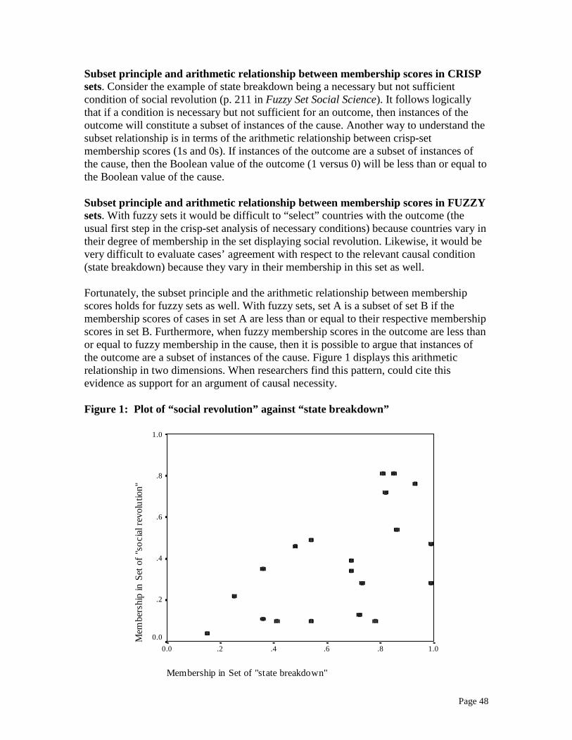
Page 48

Subset principle and arithmetic relationship between membership scores in CRISP sets. Consider the example of state breakdown being a necessary but not sufficient condition of social revolution (p. 211 in Fuzzy Set Social Science). It follows logically that if a condition is necessary but not sufficient for an outcome, then instances of the outcome will constitute a subset of instances of the cause. Another way to understand the subset relationship is in terms of the arithmetic relationship between crisp-set membership scores (1s and 0s). If instances of the outcome are a subset of instances of the cause, then the Boolean value of the outcome (1 versus 0) will be less than or equal to the Boolean value of the cause. Subset principle and arithmetic relationship between membership scores in FUZZY sets. With fuzzy sets it would be difficult to “select” countries with the outcome (the usual first step in the crisp-set analysis of necessary conditions) because countries vary in their degree of membership in the set displaying social revolution. Likewise, it would be very difficult to evaluate cases’ agreement with respect to the relevant causal condition (state breakdown) because they vary in their membership in this set as well. Fortunately, the subset principle and the arithmetic relationship between membership scores holds for fuzzy sets as well. With fuzzy sets, set A is a subset of set B if the membership scores of cases in set A are less than or equal to their respective membership scores in set B. Furthermore, when fuzzy membership scores in the outcome are less than or equal to fuzzy membership in the cause, then it is possible to argue that instances of the outcome are a subset of instances of the cause. Figure 1 displays this arithmetic relationship in two dimensions. When researchers find this pattern, could cite this evidence as support for an argument of causal necessity. Figure 1: Plot of “social revolution” against “state breakdown”

Membership in Set of "state breakdown"

1.0.8.6.4.20.0

Mem

bers

hip

in S

et o

f "so

cial

revo

lutio

n"

1.0

.8

.6

.4

.2

0.0

Page 49

The evaluation of sufficiency can be seen as a test of whether the cases displaying the causal conditions form a subset of the cases displaying the outcome. As shown above, another way to understand the subset relationship is in terms of the arithmetic relation between membership scores. In order to argue that a cause or causal combination is a sufficient for the outcome, the fuzzy membership scores in the cause should be less than or equal to the fuzzy membership scores in the outcome. Consider the following example taken from Fuzzy-Set Social Science, p. 236ff. Figure 2 displays the arithmetic relationship between the sufficient causal combinations (~cross-class • ~multiracial) against the outcome (ideological conflict). The upper-triangular plot shown in Figure 2 is a direct reflection of the fact that membership scores in the fuzzy set “race and class homogeneity” are less than or equal to membership scores in the fuzzy set “ideological conflict.” Note the important difference between the application of the subset principle to the assessment of sufficiency and its applications to the assessment of necessity. To demonstrate necessity the researcher must show that the outcome is a subset of the cause. To support an argument of sufficiency, the researcher must demonstrate that the cause is a subset of the outcome. Figure 2: Plot of “ideological conflict” against “race and class homogeneity”

Membership in "rac e and class homogeneity"

1.0.8.6.4.20.0

Mem

bser

ship

in "i

doel

ogic

al co

nflic

t"

1.0

.8

.6

.4

.2

0.0

Page 50

C) Using the Fuzzy Truth Table Algorithm This method for analyzing fuzzy sets using Truth Tables was introduced in version 2.0 of fsQCA. It is described in detail in Ragin’s (2008) Redesigning Social Inquiry: Fuzzy Sets and Beyond and in Rihoux and Ragin’s (2008) Configurational Comparative Methods: Qualitative Comparative Analysis (QCA) and Related Techniques. The fuzzy truth table algorithm can be conceptualized as a bridge with three pillars. The first pillar is the direct correspondence that exists between the rows of a crisp truth table and the coordinates of the corners of the vector space defined by fuzzy set causal conditions (see Ragin 2000). The second pillar is the assessment of the distribution of cases across different logically possible combinations of causal conditions (or sectors of the vector space). Some sectors of the vector space may have many cases with strong membership while other sectors may have cases with only weak membership. The third pillar is the assessment of the consistency of the evidence for each causal combination with the argument that it is a fuzzy subset of the outcome. The truth table algorithm involves establishing these three pillars to construct a crisp truth table, at which point the analysis proceeds similar to the crisp algorithm. This section will explain the steps involved in recording the results of multiple fuzzy set analyses in a crisp truth table and then analyzing that table. Data Fuzzy set data can be imported from other programs or created in fsQCA, as described in Chapters 1 and 2. This chapter will use the example of countries with weak class voting from Ragin (2005). The table below depicts the data sheet:

ID Country Identifier

Page 51

affluent Affluent inequality Substantial Income Inequality manufacturing Strong Manufacturing Sector unions Strong Unions weakcv Weak Class Voting Interval and ratio scale data can be converted to fuzzy set membership scores using the “calibrate” procedure described in Chapter 2 of the manual (Data Editor) and in Ragin (2008). Analysis The truth table algorithm incorporates a two-stage analytic procedure. The first step consists of creating a truth table from the fuzzy data, which includes specifying the outcome for each configuration and determining which configurations to include in the analysis. The second step involves specifying the causal conditions and outcomes to minimize. These steps must be performed in conjunction and both must be performed for each separate analysis. In order to specify the sets to be used in the analysis, choose: Analyze Truth Table Algorithm… The following window will open:

Page 52

Identify and highlight the variable you want to use as the outcome and transfer it into the Outcome field by clicking Set.

Choose causal conditions one at a time and click them over to the Causal Conditions

field by clicking Add. Check the box next to “Show solution cases in output” and choose the variable that

signifies your caseIDs. Click on the Okay button and the following window containing the truth table will

appear:

The truth table will have 2k rows (where k represents the number of causal conditions),

reflecting all possible combinations of causal conditions. The 1s and 0s indicate the different corners of the vector space defined by the fuzzy set causal conditions. For each row, a value for each of the following variables is created:

number the number of cases with greater than 0.5 membership in that corner of the vector space. Shown in parentheses is the cumulative percentage of cases, beginning with the most populated sector of the vector space

Page 53

raw consist. the degree to which membership in that corner of the vector space is a consistent subset of membership in the outcome. (For crisp sets, this is the proportion of cases in a given crisp truth table row that display the outcome.)

PRI consist. an alternative measure of consistency for fuzzy sets based on a quasi proportional reduction in error calculation. (In crisp sets this will be equal to raw consist).

SYM consist. an alternative measure of consistency for fuzzy sets based on a symmetrical version of PRI consistency.

Note that the column labeled as the outcome (weakcv in this example) is blank. It is up to the investigator to determine the outcome for each configuration and to enter it into the spreadsheet using the following procedure. The researcher must begin by developing a rule for classifying some configurations

(vector spaces corners) as relevant and others as irrelevant, based on the number of cases residing in each sector of the vector space defined by the causal conditions. This is accomplished by selecting a frequency threshold based on the number of cases with greater than 0.5 membership in each configuration, as shown in the number column. When the total N (number of cases) is relatively small, the frequency threshold should be 1 or 2. When the total N is large, a more substantial threshold should be used. It is very important to examine the distribution of cases across conditions, to identify the most populated sectors of the vector space. In general, the configurations selected should capture at least 75-80% of the cases.

Cases can be sorted by their frequency (ascending or descending) by clicking on the

number column heading. After sorting and selecting a threshold, delete all rows that do not meet the threshold.

If the cases have been sorted in a descending order according to number, click on the first case that falls below the threshold and then choose:

Edit Delete current row to last row… If cases have not been sorted then those cases that do not meet the threshold can be deleted individually by selecting the row and then choosing: Edit Delete current row… The next step is to distinguish configurations that are consistent subsets of the outcome

from those that are not. This determination is made using the measures of set-theoretic consistency reported in the raw consist, PRI, and/or SYM columns. Values below 0.80 in the raw consist column indicate substantial inconsistency. It is useful to sort the consistency scores in descending order to evaluate their distribution (this should be done after removing rows that fail to meet the frequency threshold). Sorting is

Page 54

accomplished by clicking on the raw consist, PRI, or SYM column heading (make sure the arrow, which appears when you click on the column heading, is pointing down).

Identify any gaps in the upper range of consistency that might be useful for establishing a consistency threshold. Keep in mind that it is always possible to examine several different thresholds and assess the consequences of lowering and raising the consistency cut-off. It is now necessary to indicate which configurations exhibit the outcome and which do

not. Place a 1 in the outcome column (weakcv in this example) for each configuration whose consistency level meets and/or exceeds the threshold. Place a 0 in the outcome column for each configuration whose consistency level does not meet the consistency threshold.

Alternatively, use the “Delete and code” function to automate this process. Select: Edit Delete and code… In the first field, the frequency threshold is selected. The default number of cases is 1, but may be changed by typing the selected frequency threshold into the field. In the second field, the consistency threshold (raw consist.) is selected. The default consistency is 0.8, but this may be changed by typing the selected consistency threshold into the field. Click “OK.” The program will delete rows where the frequency threshold is not met, and will code the outcome as 0 or 1 depending on the selected consistency threshold. The following window displays the truth table that would appear after

1. applying a frequency threshold of 1 to the data and eliminating configurations that do not have any observations (8 configurations) 2. selecting a consistency threshold of 0.8 and placing a 1 in the weakcv column for configurations with 0.8 consistency or greater (5 configurations) and a 0 for cases

with lower consistency (3 configurations)

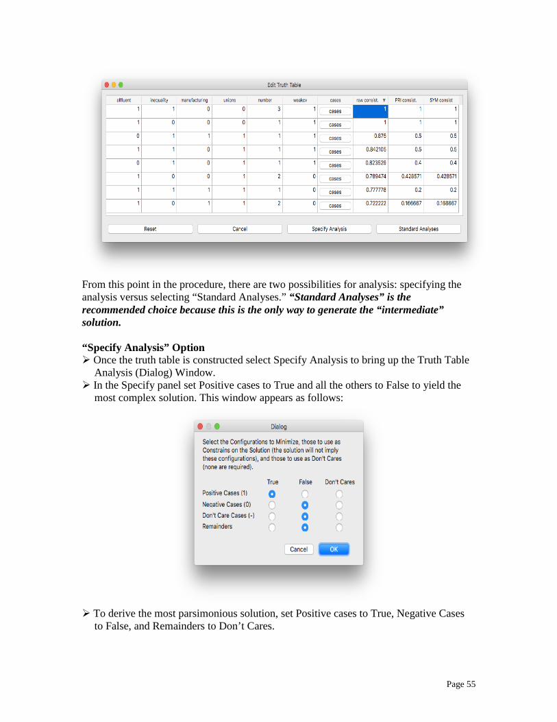
Page 55

From this point in the procedure, there are two possibilities for analysis: specifying the analysis versus selecting “Standard Analyses.” “Standard Analyses” is the recommended choice because this is the only way to generate the “intermediate” solution. “Specify Analysis” Option Once the truth table is constructed select Specify Analysis to bring up the Truth Table

Analysis (Dialog) Window. In the Specify panel set Positive cases to True and all the others to False to yield the

most complex solution. This window appears as follows:

To derive the most parsimonious solution, set Positive cases to True, Negative Cases

to False, and Remainders to Don’t Cares.

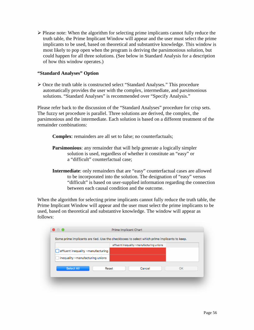
Page 56

Please note: When the algorithm for selecting prime implicants cannot fully reduce the truth table, the Prime Implicant Window will appear and the user must select the prime implicants to be used, based on theoretical and substantive knowledge. This window is most likely to pop open when the program is deriving the parsimonious solution, but could happen for all three solutions. (See below in Standard Analysis for a description of how this window operates.)

“Standard Analyses” Option Once the truth table is constructed select “Standard Analyses.” This procedure

automatically provides the user with the complex, intermediate, and parsimonious solutions. “Standard Analyses” is recommended over “Specify Analysis.”

Please refer back to the discussion of the “Standard Analyses” procedure for crisp sets. The fuzzy set procedure is parallel. Three solutions are derived, the complex, the parsimonious and the intermediate. Each solution is based on a different treatment of the remainder combinations: Complex: remainders are all set to false; no counterfactuals; Parsimonious: any remainder that will help generate a logically simpler solution is used, regardless of whether it constitute an “easy” or a “difficult” counterfactual case; Intermediate: only remainders that are “easy” counterfactual cases are allowed to be incorporated into the solution. The designation of “easy” versus “difficult” is based on user-supplied information regarding the connection between each causal condition and the outcome. When the algorithm for selecting prime implicants cannot fully reduce the truth table, the Prime Implicant Window will appear and the user must select the prime implicants to be used, based on theoretical and substantive knowledge. The window will appear as follows:

Page 57

Prime implicants (PIs) are product terms that are produced using minimization rules (e.g. rules that combine rows that differ on only one cause if they have the same output value). For example: ABC combines with AbC to produce AC. AC, therefore, is the prime implicant that covers the two primitive Boolean expressions ABC and AbC. In other words, ABC and AbC are subsets of AC, or AC implies ABC and AbC. Often, though, there are more reduced prime implicants than are needed to cover all the original primitive expressions and the user has the option to choose from among those that are “logically tied” using the prime implicant chart. (For a more comprehensive discussion of the use of Prime Implicants, refer to The Comparative Method page 95.)

To choose prime implicants (PIs), the program employs an algorithm that attempts to reduce the table until no further simplification is possible, beginning with essential PIs (which uniquely cover specific rows in the truth table) that must appear in the solution. If the algorithm is run and the table cannot be fully reduced, the user may select the PIs to be used, based on theoretical and substantive knowledge. The Prime Implicant Chart tab displays the possible prime implicants for the user to choose. Each column in the chart represents a different truth table row that is covered by more than one prime implicant. The “Data” field across the top displays the truth table row in question (the one that needs to be covered). The “Prime” field on the left-hand side describes the PI that the user may select. Each row in the chart represents one PI that may be selected. A PI is selected by clicking on the cell in the first column.

After clicking on the desired cell or cells, press OK to run the analysis.

D) Output for “Specify Analysis” Option Once the truth table has been minimized, the main window will show you the following output. The output shown is for the most complex solution, obtained by using the “Specify Analysis” option as described above.

Page 58

The first part of the output describes the data of the Truth Table Analysis. The first two rows indicate the file directory and the model you specified. Then, the output displays what kind of algorithm you used.

The last part of the output shows the Truth Table Solution of your analysis. First, frequency and consistency cutoffs are listed. This is followed by the solution(s). When the “Specify Analysis” option is selected, there will be one Truth Table Solution section. When “Standard Analyses” is selected, three solution sections will be provided (complex, parsimonious and intermediate). In this example, the solution for the most complex solution was reported, with weak class voting as a product of three configurations.

The first two lines list the frequency and consistency cutoffs. The consistency cutoff will list the lowest consistency value above the cut-off value specified by the user. Here, 0.8 was given as the consistency cutoff, and the lowest actual value above 0.8 was 0.823529. The solution provides a line for each separate path to the outcome (in this example three paths exist). The output also computes the consistency and coverage for each solution term and the solution as a whole (these computations are discussed below). The output for the most parsimonious solution of this same truth table is:

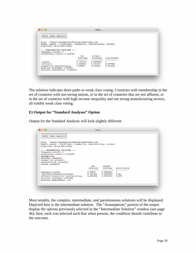
Page 59

The solution indicates three paths to weak class voting. Countries with membership in the set of countries with not-strong unions, or in the set of countries that are not affluent, or in the set of countries with high income inequality and not strong manufacturing sectors, all exhibit weak class voting. E) Output for “Standard Analyses” Option Output for the Standard Analysis will look slightly different:

Most notably, the complex, intermediate, and parsimonious solutions will be displayed. Depicted here is the intermediate solution. The “Assumptions” portion of the output display the options previously selected in the “Intermediate Solution” window (see page 46); here, each was selected such that when present, the condition should contribute to the outcome.

Page 60

In this solution, weak class voting is a product of three pathways – high membership in the set of affluent countries and weak membership in the set of countries with strong unions; weak membership in the set of affluent countries, high membership in the set of unequal countries, and high membership in the set of countries with strong unions; as well as high membership in the set of affluent countries, high membership in the set of unequal countries, and weak membership in the set of manufacturing countries. F) Consistency and Coverage The output includes measures of coverage and consistency for each solution term and for the solution as a whole. Consistency (with sufficiency) measures the degree to which solution terms and the solution as a whole are subsets of the outcome. Coverage measures how much of the outcome is covered (or explained) by each solution term and by the solution as a whole. These measures are computed by examining the original fuzzy data set in light of the solution (composed of one or more solution terms). The degree to which cases in the original dataset have membership in each solution term and in the outcome form the basis of consistency and coverage measures. More specifically, consider the following data table with three causal conditions (A, B, and C) and an outcome (Y) all measured as fuzzy sets. Causal Condition Membership

Outcome Membership Solution Membership Consistency Calculations

A B C Y A*B A*C A*B + A*C CA*B CA*C CA*B + A*C

.8 .9 .8 .9 .8 .8 .8 .8 .8 .8

.6 .7 .4 .8 .6 .4 .6 .6 .4 .6

.6 .7 .2 .7 .6 .2 .6 .6 .2 .6

.6 .6 .3 .7 .6 .3 .6 .6 .3 .6

.8 .3 .7 .8 .3 .7 .7 .3 .7 .7

.6 .1 .7 .9 .1 .6 .6 .1 .6 .6

.7 .4 .2 .3 .4 .2 .4 .3 .2 .3

.2 .9 .9 .1 .2 .2 .2 .1 .1 .1

.1 .6 .2 .2 .1 .1 .1 .1 .1 .1

.2 .1 .7 .3 .1 .2 .2 .1 .2 .2

.3 .1 .3 .3 .1 .3 .3 .1 .3 .3

.1 .2 .3 .2 .1 .1 .1 .1 .1 .1 Sum: 6.2 4.0 4.1 5.2 3.8 4.0 5.0

The relevant output for this analysis is shown below. The solution is comprised of two terms: A*B + A*C. To calculate consistency and coverage, several intermediate values must be calculated first. Membership in the outcome (ΣY) is the sum of outcome membership scores across all cases in the data. A case’s membership in each solution term is computed as the minimum of the cases membership in each causal condition of the term. Membership in the first solution term (ΣA*B) is the sum of membership in that solution term across all cases. Similarly, membership in the second solution term (ΣA*C) is the sum of membership in that solution term across all cases. Membership in the

Page 61

solution (Σ (A*B + A*C) is defined as the maximum of a case’s membership across the solution terms. raw unique coverage coverage consistency ---------- ---------- ----------- A*B+ 0.612903 0.161290 0.950000 A*C 0.645161 0.193548 0.975610 solution coverage: 0.806452 solution consistency: 0.961538

Consistency measures the degree to which membership in each solution term is a subset of the outcome. Consistency is computed by first computing the consistency of each case. For any solution term, a case is consistent if membership in the solution term is less than or equal to membership in the outcome. If a case’s membership in the solution term is greater than its membership in the outcome (i.e., it is inconsistent), then the case is given a score that equals its membership in the outcome. These scores are then summed (yielding Σ CA*B) and divided by the sum of memberships in the solution term (ΣA*B). Thus, consistency for the first solution term is Σ CA*B / ΣA*B = 3.8/4 = .95 and for the second solution term is 4.0/4.1 = .976. Solution Consistency measures the degree to which membership in the solution (the set of solution terms) is a subset of membership in the outcome. The maximum of each case’s membership across solution terms max(A*B + A*C) is compared to membership in the outcome. If membership in the solution is less than or equal to membership in the outcome, then the case is given a score that equals its membership in the solution term. If membership in the solution term if greater than membership in the outcome (i.e., if it is inconsistent), then the case is given the outcome scores (the lower of the two scores). These scores are summed and then divided by the sum of memberships in the solution term (Σ C(A*B + A*C) / Σ(A*B + A*C). The consistency for the solution in this example is 5.0/5.2 = .962. Solution coverage measures the proportion of memberships in the outcome that is explained by the complete solution. The consistent membership scores are summed across cases and then divided by the sum of the membership in the outcome: (ΣC(A*B + A*C) / ΣY) = 5/6.2 = .806. Raw coverage measures the proportion of memberships in the outcome explained by each term of the solution. Raw coverage is computed for each solution term from the original data by dividing the sum of consistent membership in the solution term by the sum of membership in the outcome. Raw coverage for the first solution term is ΣCA*B / ΣY = 3.8/6.2 = .613 and for the second term is 4.0/6.2 = .645. Unique coverage measures the proportion of memberships in the outcome explained solely by each individual solution term (memberships that are not covered by other solution terms). This is computed by first removing the term from the solution and computing solution coverage. In this example, solution coverage after removing the first

Page 62

solution term (ΣCA*B) is simply ΣCA*C (with n solution terms the reduced solution will contain n-1 solution terms). The reduced coverage term is then divided by the full solution coverage and subtracted from the raw coverage to give the unique coverage for the omitted solution term. For the first solution term (ΣCA*B) unique coverage equals: (ΣC(A*B + A*C) / ΣY) - (ΣCA*C / ΣY) = (5.0/6.2) – (4.0/6.2) = .161. Unique coverage for the second term equals (5.0/6.2) – (3.8/6.2) = .194.