Embed Size (px)
Citation preview

.
User's Guide for the Emissions Modeling System for Hazardous Air Pollutants (EMS-HAP) Version 3.0

This page intentionally blank

EPA-454/B-03-006
August 2004
User's Guide for the Emissions Modeling System for Hazardous Air Pollutants (EMS-HAP) Version 3.0
By:
Madeleine Strum, Ph.D. U.S. Environmental Protection Agency
Office of Air Quality Planning and Standards Emissions, Monitoring and Analysis Division
Research Triangle Park, NC
And, Under Contract to the U.S. Environmental Protection Agency,
Richard Mason* and James Thurman, Ph.D. CSC
Contract No. IAG47939482-01 Work Order No. 22.4
*Currently with the National Oceanic and Atmospheric Agency (NOAA) on Assignment to the U.S. EPA, Office of Air Quality Planning and Standards, Emissions, Monitoring and Analysis
Division
U.S. Environmental Protection Agency Office of Air Quality Planning and Standards Emissions, Monitoring and Analysis Division
Research Triangle Park, North Carolina

DISCLAIMER
The information in this document has been reviewed in accordance with the U.S. EPA administrative review policies and approved for publication. Mention of trade names or commercial products does not constitute endorsement or recommendation for their use. The following trademarks appear in this document: UNIX is a registered trademark of AT&T Bell Laboratories. SAS® is a registered trademark of SAS Institute. SUN is a registered trademark of Sun Microsystems, Inc.

TABLE OF CONTENTS
CHAPTER 1 Introduction .......................................................................................................... 1-1
1.1 What is EMS-HAP? ....................................................................................................... 1-1 1.2 Who are the users of EMS-HAP? .................................................................................. 1-3
1.3 What are the main features of EMS-HAP?.................................................................... 1-3 1.4 Why does EMS-HAP Version 3.0 support two inventory formats for non-point
sources? .......................................................................................................................... 1-8 1.5 How do I prepare my inventories for EMS-HAP if I am starting with the NEI? .......... 1-9 1.6 How do I use this guide?.............................................................................................. 1-10 1.7 Quick-start for ASPEN: Instructions for using EMS-HAP to prepare emission
inputs for the ASPEN model........................................................................................ 1-11 1.8 Quick-start for ISCST3: Instructions for using EMS-HAP to prepare emission
inputs for the ISCST3 model........................................................................................ 1-15 CHAPTER 2 County Emissions Processing: The County Point and Aircraft Extraction Program (COPAX)....................................................................................................................... 2-1
2.1 What is the function of COPAX? .................................................................................. 2-2 2.1.1 COPAX allocates county- level emissions, such as aircraft, to specific locations 2-5
2.1.2 COPAX prepares the allocated emissions for the point source processing programs.................................................................................................................. 2-6
2.1.3 COPAX assigns the additional variables needed to process the allocated emissions (e.g., aircraft) as ISCST3 area sources when processing data for ISCST3 only............................................................................................................ 2-8
2.1.4 If the county-level inventory contains both onroad and nonroad sources, COPAX splits the inventory into onroad and nonroad inventories ........................ 2-9 2.1.5 For non-point processing, COPAX assigns a spatial surrogate for each source
category for subsequent spatial allocation............................................................ 2-10 2.1.6 For non-point processing, COPAX gap fills or reassigns a code to each source
category for matching to temporal profiles........................................................... 2-11 2.2 How do I run COPAX?................................................................................................ 2-12
2.2.1 Prepare your county- level source inventory for input into COPAX................... 2-12 2.2.2 Prepare your point source inventory for input into COPAX .............................. 2-14 2.2.3 Determine whether you need to modify the ancillary input files for COPAX ... 2-16 2.2.4 Prepare your batch file ........................................................................................ 2-19 2.2.5 Execute COPAX ................................................................................................. 2-21
2.3 How do I know my run of COPAX was successful? ................................................... 2-21 2.3.1 Check your SAS® log file ................................................................................... 2-21 2.3.2 Check your SAS® list file ................................................................................... 2-22 2.3.3 Check other output files from COPAX............................................................... 2-23
CHAPTER 3 Point Source Processing: The Data Quality Assurance Program (PtDataProc) .. 3-1
3.1 What is the function of PtDataProc? .............................................................................. 3-2 3.1.1 PtDataProc quality assures point source location data ......................................... 3-5

TABLE OF CONTENTS (continued)
ii
3.1.2 PtDataProc quality assures stack parameters; defaults if missing or out-of-range........................................................................................................... 3-12
3.1.3 PtDataProc removes inventory variables and records not necessary for further processing (inventory windowing) ....................................................................... 3-13
3.2 How do I run PtDataProc? ............................................................................................ 3-14 3.2.1 Prepare your point source inventory for input into PtDataProc.......................... 3-14 3.2.2 Determine whether you need to modify the ancillary input files for
PtDataProc ............................................................................................................ 3-18 3.2.3 Prepare your batch file ........................................................................................ 3-19 3.2.4 Execute PtDataProc............................................................................................. 3-23
3.3 How do I know my run of PtDataProc was successful?. .............................................. 3-24 3.3.1 Check your SAS® log file .................................................................................... 3-24 3.3.2 Check your SAS® list file .................................................................................... 3-24 3.3.3 Check other output files from PtDataProc ........................................................... 3-25
CHAPTER 4 Point Source Processing: The Model-Specific Program (PtModelProc)............. 4-1
4.1 What is the function of PtModelProc? ........................................................................... 4-2 4.1.1 PtModelProc selects pollutants, groups and/or partitions pollutants, and assigns
model-specific pollutant characteristics.................................................................. 4-3 4.1.2 PtModelProc speciates pollutants by inventory source characteristics (MACT,
SCC, or SIC codes) ................................................................................................. 4-4 4.1.3 PtModelProc assigns urban/rural dispersion parameters when processing data for
ASPEN only............................................................................................................ 4-5 4.1.4 PtModelProc assigns vent type and building parameters ..................................... 4-5
4.2 How do I run PtModelProc? ...................................................................................... 4-7 4.2.1 Prepare your point source inventory for input into PtModelProc ......................... 4-7 4.2.2 Determine whether you need to modify the ancillary input files for
PtModelProc.......................................................................................................... 4-10 4.2.3 Modify the General HAP table input files .......................................................... 4-12 4.2.4 Modify the Specific HAP table input file ........................................................... 4-19 4.2.5 Prepare your batch file ........................................................................................ 4-23 4.2.6 Execute PtModelProc.......................................................................................... 4-25
4.3 How do I know my run of PtModelProc was successful? ........................................... 4-25 4.3.1 Check your SAS® log file ................................................................................... 4-25 4.3.2 Check your SAS® list file ................................................................................... 4-26 4.3.3 Check other output files from PtModelProc ....................................................... 4-26
CHAPTER 5 Point Source Processing: The Temporal Allocation Program (PtTemporal) ..... 5-1
5.1 What is the function of PtTemporal? ......................................................................... 5-2 5.1.1 PtTemporal assigns a temporal profile to each emission record............................ 5-5 5.1.2 PtTemporal uses the hourly profiles to produce eight 3-hour emission rates when
processing data for ASPEN only ............................................................................ 5-5

TABLE OF CONTENTS (continued)
iii
5.1.3 PtTemporal uses the hourly, day, and seasonal profiles to produce 288 emission rates when processing data for ISCST3 only .......................................................... 5-6
5.2 How do I run PtTemporal ............................................................................................ 5-10 5.2.1 Prepare your point source inventory for input into PtTemporal......................... 5-10 5.2.2 Determine whether you need to modify the ancillary input files for
PtTemporal............................................................................................................ 5-15 5.2.3 Modify the temporal allocation factor file (keyword TAF) ................................ 5-16 5.2.4 Modify the cross-reference files used to link inventory records to the temporal
allocation factor file (ancillary file keywords SCCLINK, SICLINK, and MACTLINK). ....................................................................................................... 5-17
5.2.5 Prepare your batch file ........................................................................................ 5-17 5.2.6 Execute PtTemporal............................................................................................ 5-19
5.3 How Do I Know My Run of PtTemporal Was Successful? ........................................ 5-19 5.3.1 Check your SAS® log file ................................................................................... 5-19 5.3.2 Check your SAS® list file ................................................................................... 5-19 5.3.3 Check other output files from PtTemporal ......................................................... 5-19
CHAPTER 6 Point Source Processing: The Growth and Control Program (PtGrowCntl) ...... 6-1
6.1 What is the function of PtGrowCntl? ........................................................................... 6-2 6.1.1 PtGrowCntl determines a projection scenario for each record in the PROJECT
ancillary file ............................................................................................................ 6-4 6.1.2 For each scenario, PtGrowCntl assigns and applies growth factors to project
emissions due to growth ......................................................................................... 6-6 6.1.3 For each scenario, PtGrowCntl assigns MACT-based emission reduction
information ............................................................................................................. 6-7 6.1.4 For each scenario, PtGrowCntl assigns user-defined emission reduction
information .......................................................................................................... 6-10 6.1.5 For each scenario, PtGrowCntl combines MACT-based and user-defined
emission reduction information and applies to grown emissions to project emissions for that scenario .................................................................................... 6-13
6.2 How do I run PtGrowCntl? .......................................................................................... 6-16 6.2.1 Prepare your point source inventory for input into PtGrowCntl......................... 6-16 6.2.2 Determine whether you need to modify the ancillary input files for
PtGrowCntl ........................................................................................................... 6-20 6.2.3 Modify the growth factor input files (GFSITE, GFMACT, GFSIC, and
GFSCC)................................................................................................................. 6-22 6.2.4 Modify the MACT-based emission reduction information files (MACTGEN
and SPECFILE) .................................................................................................... 6-23 6.2.5 Develop the user-defined emission reduction information files (USERFILE
and CNTYUR) ...................................................................................................... 6-24 6.2.6 Prepare your batch file ........................................................................................ 6-24 6.2.7 Execute PtGrowCntl ........................................................................................... 6-27

TABLE OF CONTENTS (continued)
iv
6.3 How Do I Know My Run of PtGrowCntl Was Successful? ........................................ 6-27 6.3.1 Check your SAS® log file ................................................................................... 6-27 6.3.2 Check your SAS® list file ................................................................................... 6-27 6.3.3 Check other output files from PtGrowCntl......................................................... 6-28
CHAPTER 7 Point Source Processing: The Final Format Program For ASPEN (PtFinal_ASPEN)......................................................................................................................... 7-1
7.1 What is the function of PtFinal_ASPEN?...................................................................... 7-2 7.1.1 PtFinal_ASPEN assigns ASPEN source groups used in the ASPEN model
output ..................................................................................................................... 7-4 7.1.2 PtFinal_ASPEN converts temporally allocated emissions from tons/year to
grams/second for each of the eight 3-hour periods................................................. 7-5 7.1.3 PtFinal_ASPEN creates ASPEN input files, a column formatted text file and
a SAS® file ........................................................................................................... 7-5 7.2 How do I run PtFinal_ASPEN? ................................................................................ 7-7
7.2.1 Prepare your point source inventory for input into PtF inal_ASPEN ................. 7-7 7.2.2 Determine whether you need to modify the ancillary input files for
PtFinal_ASPEN ................................................................................................. 7-10 7.2.3 Modify the source group assignment files (ancillary file keywords MACTGRP,
SCCGRP, and SICGRP) .................................................................................... 7-10 7.2.4 Prepare your batch file ......................................................................................... 7-11 7.2.5 Execute PtFinal_ASPEN ..................................................................................... 7-13
7.3 How do I know my run of PtFinal_ASPEN was successful? ................................ 7-13 7.3.1 Check your SAS® log file ................................................................................... 7-13 7.3.2 Check your SAS® list file ................................................................................... 7-14 7.3.3 Check other output files from PtFinalASPEN .................................................... 7-14
CHAPTER 8 Point Source Processing: The Final Format Program For ISCST3 (PtFinal_ISCST3) ........................................................................................................................ 8-1
8.1 What is the function of PtFinal_ISCST3? .................................................................... 8-2 8.1.1 PtFinal_ISCST3 assigns source groups used in the ISCST3 model output ........ 8-4 8.1.2 PtFinal_ISCST3 assigns default release parameters in order to model fugitive
sources and horizontal stacks as ISCST3 volume sources .................................. 8-5 8.1.3 PtFinal_ISCST3 assigns available particulate size and gas deposition data by
pollutant or by combination of SCC and pollutant ................................................ 8-6 8.1.4 PtFinal_ISCST3 removes emission sources outside your modeling domain ... 8-7 8.1.5 PtFinal_ISCST3 assigns available emission source elevation data .................... 8-8 8.1.6 PtFinal_ISCST3 assigns source identification codes needed for the ISCST3 SO
pathway section files ............................................................................................ 8-9 8.1.7 PtFinal_ISCST3 converts temporally allocated emissions from tons/hour to the
necessary units for each source for each of the 288 emission rates ..................... 8-9 8.1.8 PtFinal_ISCST3 adjusts UTM coordinates of emission sources ........................ 8-10

TABLE OF CONTENTS (continued)
v
8.1.9 PtFinal_ISCST3 creates SO pathway section of the ISCST3 run stream and include files........................................................................................................... 8-11
8.2 How do I run PtFinal_ISCST3? ................................................................................... 8-13 8.2.1 Prepare your point source inventory for input into PtFinal_ISCST3 ................. 8-13 8.2.2 Determine whether you need to modify the ancillary input files for
PtFinal_ISCST3 .................................................................................................... 8-15 8.2.3 Modify the source group assignment files (ancillary file keywords MACTGRP,
SCCGRP, and SICGRP) ...................................................................................... 8-16 8.2.4 Develop the particle size distribution, gas deposition, and terrain elevation files
(ancillary files DEFPART, SCCPART, DEFGAS, and ELEVDAT) .................. 8-17 8.2.5 Prepare your batch file ........................................................................................ 8-17 8.2.6 Execute PtFinal_ISCST3 ............................................................................. 8-20
8.3 How Do I Know My Run of PtFinal_ISCST3 Was Successful? ................................. 8-21 8.3.1 Check your SAS® log file ................................................................................... 8-21 8.3.2 Check your SAS® list file ................................................................................... 8-21 8.3.3 Check other output files from PtFinal_ISCST3 ............................................ 8-21
CHAPTER 9 County-Level Non-Point and Mobile Source Processing: The County-Level Source Processor (CountyProc) ................................................................................................... 9-1
9.1 What is the Function of CountyProc? ............................................................................. 9-2 9.1.1 CountyProc determines overall program flow and file outputs based on user
options ..................................................................................................................... 9-5 9.1.2 CountyProc selects pollutants, groups and/or partitions pollutants, and assigns
their characteristics, and speciates pollutants by inventory source......................... 9-7 9.1.3 CountyProc assigns source groups and source type ............................................ 9-8 9.1.4 CountyProc spatially allocates county- level emissions (if necessary) ............... 9-10 9.1.5 CountyProc temporally allocates emissions (if necessary)................................. 9-14 9.1.6 CountyProc assigns ASPEN-specific modeling parameters- for ASPEN
processing only ..................................................................................................... 9-16 9.1.7 CountyProc projects emissions to (a) future year(s) ........................................... 9-16 9.1.8 CountyProc converts temporally allocated emissions from tons/year to
grams/second for each of the eight 3-hour periods when processing data for ASPEN only........................................................................................................................ 9-25
9.1.9 CountyProc creates ASPEN input files, column formatted text and SAS® files when processing data for ASPEN only................................................................. 9-25
9.1.10 CountyProc creates the SAS® file used as input to CountyFinal when processing data for ISCST3 .................................................................................................... 9-27
9.1.11 CountyProc creates SAS® file when processing county-level projected emissions data (GCFLAG=0) ................................................................................................ 9-27
9.2 How do I run CountyProc? ........................................................................................... 9-28 9.2.1 Prepare your non-point and mobile source emission inventory files for input into
CountyProc............................................................................................................ 9-28

TABLE OF CONTENTS (continued)
vi
9.2.2 Determine whether you need to modify the ancillary input files for CountyProc............................................................................................................ 9-29
9.2.3 Modify the HAP table input files ...................................................................... 9-33 9.2.4 Modify the files that assign non-point and mobile source categories to source
groups and source type (EMISBINS and CNTYUR) ........................................... 9-34 9.2.5 Modify the source category-to-spatial surrogate cross-reference (SURRXREF)
and optionally, the file that provides spatial surrogate descriptions (SURRDESC) ....................................................................................................... 9-35
9.2.6 Modify the temporal allocation factor file (TAFFILE) .................................... 9-35 9.2.7 Modify the growth factors and emission reduction information files ............... 9-36 9.2.8 Prepare your batch file ........................................................................................ 9-37 9.2.9 Execute CountyProc............................................................................................ 9-40
9.3 How Do I Know My Run of CountyProc Was Successful? ......................................... 9-40 9.3.1 Check your SAS® log file .................................................................................. 9-40 9.3.2 Check your SAS® list file .................................................................................. 9-41 9.3.3 Check other output files ...................................................................................... 9-44
CHAPTER 10 County-Level Non-Point and Mobile Source Processing: The Final Format Program (CountyFinal) For ISCST3 .......................................................................................... 10-1
10.1 What is the function of CountyFinal? .......................................................................... 10-2 10.1.1 CountyFinal assigns default release parameters to emission sources ............... 10-4 10.1.2 CountyFinal assigns available pollutant-specific particle size and gas
deposition data ..................................................................................................... 10-5 10.1.3 CountyFinal assigns available emission source elevation data......................... 10-5 10.1.4 CountyFinal converts each of the 288 temporally allocated emission rates and
baseline emissions to grams/sec- m2 ................................................................... 10-6 10.1.5 CountyFinal removes emission sources that are outside of modeling domain..10-7 10.1.6 CountyFinal assigns source identification codes needed for the ISCST3 SO
pathway section files ........................................................................................... 10-7 10.1.7 CountyFinal calculates UTM coordinates for the tract-level approach and
adjusts UTM coordinates of emission sources for both approaches ................... 10-7 10.1.8 CountyFinal creates include files for the SO pathway section of the ISCST3
run stream............................................................................................................ 10-8 10.1.9 CountyFinal creates text files containing source identification information
for the source groups for inclusion in the SO pathway section of the ISCST3 run stream.......................................................................................................... 10-10
10.2 How do I run CountyFinal? ..................................................................................... 10-10 10.2.1 Prepare your point source inventory for input into CountyFinal.................... 10-10 10.2.2 Determine whether you need to modify the ancillary input files for
CountyFinal....................................................................................................... 10-12 10.2.3 Develop the particle size distribution, gas deposition, terrain elevation, and tract
vertices files (DEFPART, DEFGAS, ELEVDAT and TRACTFILE )............. 10-11

TABLE OF CONTENTS (continued)
vii
10.2.4 Prepare your batch file .................................................................................... 10-13 10.2.5 Execute CountyFinal....................................................................................... 10-15
10.3 How Do I Know My Run of CountyFinal Was Successful? ................................... 10-15 10.3.1 Check your SAS® log file ............................................................................... 10-15 10.3.2 Check your SAS® list file ............................................................................... 10-15 10.3.3 Check other output files from CountyFinal .................................................... 10-16
References ....................................................................................................................................R-1 Appendix A EMS-HAP Ancillary File Formats ......................................................................... A-1 Appendix B EMS-HAP Sample Batch Files ...............................................................................B-1 Appendix C EMS-HAP Ancillary File Development................................................................. C-1

This page intentionally blank

ix
LIST OF TABLES Table 2-1. Variables Assigned to Point Sources Extracted from County- level Emissions ........ 2-7 Table 2-2. Additional Variables Required to Process Allocated County-level Emissions as ISCST3 Area Sources ............................................................................................ 2-9 Table 2-3. Required Variables in COPAX County-level SAS® Input File when Source Inventory is Non-Point (keyword EMISTYPE=AR).............................................. 2-13 Table 2-4. Required Variables in COPAX County-level SAS® Input File when Source Inventory is Nonroad or Onroad Mobile (keyword EMISTYPE=MV)................... 2-13 Table 2-5. Variables Required in COPAX Input Point Source Inventory SAS® File ............. 2-15 Table 2-6. Additional Variables Required for COPAX Input Point Source Inventory SAS® File when Processing ISCST3 Area or Volume Sources ........................................ 2-16 Table 2-7. Ancillary Input File Keywords for COPAX when Processing Non-point Emissions (keyword EMISTYPE = AR)................................................................................... 2-18 Table 2-8. Ancillary Input File Keywords for COPAX when Processing Nonroad Mobile Emissions (keyword EMISTYPE = MV) .............................................................. 2-19 Table 2-9. Keywords in the COPAX Batch File for Either ASPEN or ISCST3 ...................... 2-20 Table 3-1. PtDataProc Functions for QA of Point Source Location Data ................................. 3-5 Table 3-2. Assignment of LLPROB Diagnostic Flag Variable .................................................. 3-7 Table 3-3. Resolutions in Discrepancy Between Alternate and Inventory FIPS Code (Processing for ASPEN only) .................................................................................. 3-10 Table 3-4. Assignment of Diagnostic Flag Variables LFLAG and FIPFLAG (Processing for ASPEN only) ........................................................................................................... 3-11 Table 3-5. Assignment of Stack Parameter Defaulting Diagnostic Flag Variables.................. 3-13 Table 3-6. Variables Required for PtDataProc Input Point Source Inventory SAS® File ........ 3-16 Table 3-7. Additional Variables for PtDataProc Input Point Source Inventory SAS® File when Processing ISCST3 Area or Volume Sources ............................................... 3-17 Table 3-8. Ancillary Input File Keywords for PtDataProc ....................................................... 3-18 Table 3-9. Keywords for Selecting PtDataProc Functions ....................................................... 3-19 Table 3-10. Keywords in the PtDataProc Batch File When Processing Data for ASPEN ....... 3-20 Table 3-11. Keywords in the PtDataProc Batch File When Processing Data for ISCST3 ....... 3-22 Table 3-12. Additional QA Files Created by PtDataProc ......................................................... 3-25 Table 4-1. Hierarchy for Applying Speciation Information ...................................................... 4-5 Table 4-2. Assignment of Vent Type Variable for ASPEN Model............................................ 4-6 Table 4-3. Assignment of Default Building Height and Width for the ISCST3 Model............. 4-7 Table 4-4. Variables in the PtModelProc Input Point Source Inventory SAS® File when Processing Data for ASPEN ..................................................................................... 4-8 Table 4-5. Variables in the PtModelProc Input Point Source Inventory SAS® File when Processing Data for ISCST3 ..................................................................................... 4-9 Table 4-6. Ancillary Input File Keywords for PtModelProc .................................................... 4-11 Table 4-7. Structure of the General HAP Table ........................................................................ 4-14 Table 4-8. Sample Entries in a General HAP Table ................................................................. 4-15 Table 4-9. Directions for Partitioning or Grouping of Inventory Species ................................ 4-16 Table 4-10. Using the FACTOR Variable in the General HAP Table to Adjust Emissions .... 4-18

LIST OF TABLES (continued)
x
Table 4-11. Structure of the Specific HAP Table (keyword SPECHAP) ................................. 4-20 Table 4-12. Sample Entries in the Specific HAP Table (keyword SPECHAP) ....................... 4-21 Table 4-13. How to add records to the specific HAP table to speciate the grouped and partitioned pollutants resulting from PtModelProc’s application of the general HAP table .............................................................................................................. 4-22 Table 4-14. Example of using the SPECFX factor to Speciate Chromium Compound (CAS=136) Emissions When SIC=2431 ............................................................... 4-23 Table 4-15. Sample Entries in the Specific HAP Table (keyword SPECHAP) ....................... 4-24 Table 4-16. Keywords in the PtModelProc Batch File when Processing Data for ISCST3 ..... 4-24 Table 5-1. Variables in the PtTemporal Input Point Source Inventory SAS® File when Processing Data for ASPEN ................................................................................... 5-12 Table 5-2. Variables in the PtTemporal Input Point Source Inventory SAS® File when Processing Data for ISCST3 ................................................................................... 5-14 Table 5-3. Additional Required Variables in the PtTemporal Input Point Source Inventory SAS® File when Processing Seasona l-Hourly Data for ISCST3 ............ 5-15 Table 5-4. Ancillary Input File Keywords for PtTemporal ...................................................... 5-16 Table 5-5. Keywords in the PtTemporal Batch File when Processing Data for Either ASPEN or ISCST3 .................................................................................................. 5-18 Table 6-1. Information in the PROJECT File and Sample Values ............................................. 6-5 Table 6-2. Growth Factor Application Information and Order of Precedence ........................... 6-6 Table 6-3. Order of Precedence for MACT-based Emission Reduction Information.............. 6-10 Table 6-4. User-defined Emission Reduction Information and Order of Precedence .............. 6-12 Table 6-5. Assignment of Primary and Additional Reduction Variables ................................. 6-14 Table 6-6. Summary of Equations Used to Apply Primary Emission Reduction Information.6-15 Table 6-7. Summary of Equations used to Apply Additional Emission Reduction Information.............................................................................................................. 6-16 Table 6-8. Variables in the PtGrowCntl Input Point Source Inventory SAS® File when Processing Data for ASPEN ................................................................................... 6-17 Table 6-9. Variables in the PtGrowCntl Input Point Source Inventory SAS® File when Processing Data for ISCST3 ................................................................................... 6-19 Table 6-10. Ancillary Input File Keywords for PtGrowCntl.................................................... 6-21 Table 6-11. Regional Assignment of Growth Factors in the Growth Factor Files ................... 6-22 Table 6-12. Batch File Keywords in the PtGrowCntl for Either ASPEN or ISCST3 ............... 6-25 Table 6-13. PROJECT File Keywords for Selecting PtGrowCntl Functions ........................... 6-26 Table 7-1. Assignment of Source Groups for ASPEN model Using Source Type..................... 7-4 Table 7-2. Variables in the PtFinal_ASPEN Input Point Source Inventory SAS® File ............. 7-8 Table 7-3. Ancillary Input File Keywords for PtFinal_ASPEN ............................................... 7-10 Table 7-4. Keywords for Selecting PtFinal_ASPEN Functions ............................................... 7-11 Table 7-5. Keywords in the PtFinal_ASPEN Batch File .......................................................... 7-12 Table 7-6. Variables Added to Input Inventory in Creating the PtFinal_ASPEN Output Point Source Inventory SAS® File ................................................................................... 7-14 Table 7-7. PtFinal_ASPEN Output ASCII File Variables ........................................................ 7-15

xi
Table 8-1. Assignment of Source Groups for the ISCST3 model .............................................. 8-4 Table 8-2. Default ISCST3 Volume Source Release Parameters Assigned to Fugitive and Horizontal Emission Release Types .......................................................................... 8-6 Table 8-3. ISCST3 Deposition Algorithms and Required Information...................................... 8-6 Table 8-4. Modeling Grid Information Required by PtFinal_ISCST3 to Assign Grid Cell When Using Grid Cell Approach............................................................................... 8-7 Table 8-5. ISCST3 SO Pathway Run Stream Include Files...................................................... 8-12 Table 8-6. ISCST3 SO Pathway Include File Names ............................................................... 8-12 Table 8-7. Variables in the PtFinal_ISCST3 Input Point Source Inventory SAS® File ........... 8-13 Table 8-8. Ancillary Input File keywords for PtFinal_ISCST3 ................................................ 8-16 Table 8-9. Keywords for Selecting PtFinal_ISCST3 Functions ............................................... 8-18 Table 8-10. Keywords in the PtFinal_ISCST3 Batch File......................................................... 8-19 Table 8-11. Variables Added to Input Inventory in Creating the PtFinal_ISCST3 Output Point Source Inventory SAS® File ......................................................................... 8-23 Table 9-1. How Projection Options (PROJECT file contents) Affect CountyProc Program Flow ........................................................................................................................ 9-6 Table 9-2. Information in the PROJECT File and Sample Values ........................................... 9-19 Table 9-3. Specification of User-defined Emission Reduction Information and Order of Precedence ............................................................................................................... 9-22 Table 9-4. Assignment of Primary and Additional Control Variables ..................................... 9-23 Table 9-5. Equations Used to Apply Primary and Additional Emission Reduction Information ............................................................................................................. 9-24 Table 9-6. Variables in the CountyProc Input Non-point Source Inventory SAS® File........... 9-28 Table 9-7. Variables in the CountyProc Input Mobile Source Inventory SAS® File ............... 9-29 Table 9-8. Ancillary Input File Keywords (in the Batch File) for CountyProc ........................ 9-30 Table 9-9. Ancillary Input File Keywords in the PROJECT File for CountyProc ................... 9-32 Table 9-10. Keywords in the CountyProc Batch File ................................................................ 9-38 Table 9-11. PROJECT File Keywords for Selecting CountyProc Functions ............................ 9-39 Table 9-12. CountyProc Output File Names (located in the OUTFILES directory) ................. 9-45 Table 9-13. Format of CountyProc ASCII Data File Created when Processing Data For ASPEN ................................................................................................................... 9-46 Table 9-14. Variables Contained in CountyProc Core SAS® Output File Created When Processing Data For ASPEN ................................................................................ 9-47 Table 9-15. Variables Contained in CountyProc Extended SAS® Output File When Processing Data For ASPEN ................................................................................. 9-48 Table 9-16. Variables Contained in CountyProc Core SAS® Output File Created When Processing Data For ISCST3 ................................................................................. 9-49 Table 9-17. Variables Contained in CountyProc Extended SAS® Output File When Processing Data For ISCST3 ................................................................................. 9-50 Table 9-18. Variables Contained in CountyProc Extended SAS® Output File When Projecting County-Level Emissions (GCFLAG=0).............................................. 9-51 Table 10-1. Default ISCST3 Area Source Release Parameters and Source Dimensions ......... 10-4 Table 10-2. ISCST3 Deposition Algorithms and Required Information.................................. 10-5 Table 10-3. ISCST3 SO Pathway Run Stream Include Files.................................................... 10-9

LIST OF TABLES (continued)
xii
Table 10-4. ISCST3 Include File Names .................................................................................. 10-9 Table 10-5. Text File Names Containing Emission Source Groupings .................................. 10-10 Table 10-6. Variables in the CountyFinal Input Inventory SAS® File ................................... 10-11 Table 10-7. Ancillary Input File Keywords for CountyFinal ................................................. 10-12 Table 10-8. Keywords for Selecting CountyFinal Functions ................................................. 10-13 Table 10-9. Keywords in the CountyFinal Batch File ............................................................ 10-14 Table 10-10.Variables in the CountyFinal Output SAS® File ................................................. 10-17

xiii
LIST OF FIGURES Figure 1-1. Overview of EMS-HAP Processing for ASPEN ..................................................... 1-5 Figure 1-2. Overview of EMS-HAP Processing for ISCST3 ..................................................... 1-7 Figure 2-1. COPAX Flowchart when Processing for ASPEN and ISCST3 ............................... 2-1 Figure 2-2. COPAX Flowchart when Processing Data for ASPEN ........................................... 2-3 Figure 2-3. COPAX Flowchart when Processing Data for ISCST3 ........................................... 2-4 Figure 2-4. Example of Allocating Commercial Aircraft County-level Emissions to Discrete Locations for Point Source Processing ........................................................................................ 2-6 Figure 2-5. Relationship of ISCST3 Area Source Parameters to Center of Source ................. 2-17 Figure 3-1. Overview of PtDataProc within EMS-HAP Point Source Processing..................... 3-1 Figure 3-2. PtDataProc Flowchart when Processing Data for ASPEN ...................................... 3-3 Figure 3-3. PtDataProc Flowchart when Processing Data for ISCST3 ...................................... 3-4 Figure 4-1. Overview of PtModelProc within EMS-HAP Point Source Processing .................. 4-1 Figure 4-2. PtModelProc Flowcharts when Processing Data for ASPEN and ISCST3 ............. 4-2 Figure 5-1. Overview of PtTemporal within EMS-HAP Point Source Processing .................... 5-1 Figure 5-2. PtTemporal Flowchart when Processing Data for ASPEN...................................... 5-3 Figure 5-3. PtTemporal Flowchart when Processing Data for ISCST3 ...................................... 5-4 Figure 6-1. Overview of PtGrowCntl within EMS-HAP Point Source Processing..................... 6-1 Figure 6-2. PtGrowCntl Flowchart when Processing Data for ASPEN and ISCST3................. 6-3 Figure 7-1. Overview of PtFinal_ASPEN within EMS-HAP Point Source Processing ............ 7-1 Figure 7-2. PtFinal_ASPEN Flowchart ...................................................................................... 7-3 Figure 8-1. Overview of PtFinal_ISCST3 within EMS-HAP Point Source Processing ............ 8-1 Figure 8-2. PtFinal_ISCST3 Flowchart ...................................................................................... 8-3 Figure 8-3. PtFinal_ISCST3 Sample SO Pathway Section Output of the ISCST3 Runstream for Benzene (SAROAD = 45201) ........................................................................... 8-21 Figure 9-1. Overview of CountyProc within EMS-HAP for County-level Non-point and Mobile Source Procession for ASPEN and ISCST3 ................................................................... 9-1 Figure 9-2. CountyProc Flow chart when Procession Data for ASPEN.................................... 9-3 Figure 9-3. CountyProc Flow chart when Procession Data for ISCST3 ................................... 9-4 Figure 9-4. The Spatial Allocation Process in CountyProc ..................................................... 9-12 Figure 9-5. Non-point and Mobile Source Temporal Emissions Processing Flowchart when Processing Data for ASPEN ...................................................................................................... 9-15 Figure 9-6. Non-point and Mobile Source Temporal Emissions Processing Flowchart when Processing Data for ISCST3 ...................................................................................................... 9-15 Figure 9-7. Non-point and Mobile Source Growth and Control Projection Flowchart ........... 9-18 Figure 10-1. Overview of CountyFinal within EMS-HAP for County-level Non-point and Mobile Source Processing.......................................................................................................... 10-1 Figure 10-2. CountyFinal Flowchart........................................................................................ 10-3

xiv
DEFINITION OF ACRONYMS
AIRS EPA’s Aerometric Information Retrieval System AMS AIRS Area and Mobile System source category code for area and mobile sources
of emissions ASPEN Assessment System for Population Exposure Nationwide CAS Chemical Abstract Service EMS-HAP The Emission Modeling System for Hazardous Air Pollutants EPA United States Environmental Protection Agency ISCST3 Industrial Source Complex Short Term Model, Version 3 HAP Hazardous Air Pollutant, as defined by Section 112 of the Clean Air Act MACT Maximum Available Control Technology standards for HAP, established under
Section 112 of the Clean Air Act NAICS North American Industry Classification System NEI EPA’s National Emission Inventory NIF EPA’s NEI Input Format NTI EPA’s National Toxics Inventory OAQPS EPA’s Office of Air Quality Planning and Standards ORD EPA’s Office of Research and Development OTAQ EPA’s Office of Transportation and Air Quality SAROAD Air pollution chemical species classification system used in EPA’s initial data
base for “Storage and Retrieval of Aerometric Data” SIC Standard Industrial Classification code used for Federal economic statistics SCC AIRS Source Classification Code used for point sources of emissions SAF Spatial Allocation Factor TAF Temporal Allocation Factor

1-1
CHAPTER 1 Introduction
1.1 What is EMS-HAP? The Emissions Modeling System for Hazardous Air Pollutants (EMS-HAP) Version 3.0 is a series of computer programs, henceforth referred to as EMS-HAP, that process emission inventory data for toxic air pollutants for subsequent air quality modeling. EMS-HAP prepares the emission inputs for either the Assessment System for Population Exposure Nationwide (ASPEN) dispersion model1 or the Industrial Source Complex Short Term Version 3 (ISCST3) dispersion model.2 In addition, EMS-HAP allows you to project base-year emissions to future years for use in these air quality models. LEMS-HAP Version 3.0 code and the instructions presented in this user’s guide completely replace EMS-HAP Version 2.0. However, Appendicies D and E of the EMS-HAP Version 2.0 User’s Guide (EPA-454/B-02-001) supplement the information provided in this user’s guide. In particular, they describe the origin of some of the data supplied with EMS-HAP, and they describe national and local scale modeling applications. The key improvements in Version 3.0 are:
• the capability to run multiple projection scenarios in a single run, • the capability for chemical speciation by source category, • the generalization of the airport allocation routine so that, given the proper inputs, any
county-level source in the non-point or nonroad inventory could be assigned coordinates and modeled with the point sources
• an algorithm to use the tract-level surrogates provided with EMS-HAP for spatial allocation for the ISCST3 model and prepare the tract-level emissions as polygonal ISCST3-area sources representing the size and shape of the corresponding tracts.
In addition, an updated set of spatial surrogate ratio files is supplied with Version 3.0 to allocate county-level emissions to census tracts (based on the 2000 census) across the nation. The U.S. Environmental Protection Agency’s Office of Air Quality Planning and Standards (EPA/OAQPS), referred to hereafter as “we”, developed EMS-HAP to facilitate multiple runs of ASPEN or ISCST3 and to analyze multiple emission reduction scenarios. The EMS-HAP/ASPEN system has been used to estimate annual average ambient air quality concentrations of multiple toxic pollutants emitted from a large number of sources at a large scale (i.e., nationwide) as part of a national scale air toxics assessment.3 The EMS-HAP/ISCST3 system has been used to estimate annual ambient air quality concentrations of toxic pollutants emitted from a large number of sources on an urban scale.4 We have tailored EMS-HAP Version 3.0 to process either the July 2001 version of the 1996 National Toxics Inventory (NTI), or, Version 3 of the 1999 National Emissions Inventory (NEI).

1-2
However, you can use it for any emission inventory following the instructions in this guide. The 1996 NTI (July 2001 version) was the first comprehensive model-ready national inventory of toxics, containing site-specific estimates of hazardous air pollutants (HAPs)5, and was used in the 1996 National Scale Assessment (www.epa.gov/ttn/atw/nata). The toxics inventory, now called the National Emission Inventory (NEI), has undergone some significant formatting changes to utilize the NEI input format (NIF) version 3.0 (www.epa.gov/ttn/chief/nif/index.html). See Section 1.4 for more information on this aspect of EMS-HAP. To process data for the ASPEN and ISCST3 models, EMS-HAP Version 3.0:
C checks inventory location data, converts to latitude/longitude coordinates for ASPEN or UTM coordinates for ISCST3, defaults missing or out-of-range data for ASPEN, removes inventory records with missing or out-of-range location data when processing for ISCST3;
C checks inventory stack parameter data and defaults missing or out-of-range data; C identifies point sources, when processing for ISCST3, as one of three ISCST3 source
types: ISCST3 point, ISCST3 volume, and ISCST3 area; C groups and/or partitions individual pollutant species (e.g., groups lead oxide, lead nitrate
into a lead group; partitions lead chromate into lead and chromium groups); C where desired, further speciates individual pollutants (e.g., chromium and compounds
into hexavalent chromium) by inventory MACT, SIC, or SCC code; C facilitates the selection of pollutants and pollutant groups for modeling; C assigns building heights and widths to certain stacks; C spatially allocates county-level stationary and mobile source emissions to the census tract
level for ASPEN and to grid cells or census tracts for ISCST3 using spatial surrogates such as population;
C allocates certain county-level sources to particular locations (e.g., airports) to be modeled as point sources in ASPEN or, when processing for ISCST3, as ISCST3 area sources with specific southwest corner, horizontal and vertical dimensions and angle;
C temporally allocates annual emission rates to annually averaged (i.e., same rate for every day of the year) 3-hour emission rates to account for diurnal patterns of emissions when processing for ASPEN;
C temporally allocates annual emissions to seasonal and day-type specific hourly emission rates to account for diurnal, day-of-week and seasonal patterns in emissions and imparts a a day-type variation to MOBILE6.2-based seasonal and hourly emissions when processing for ISCST3;
C assigns reactivity and particulate size classes to the pollutants when processing for ASPEN, to allow ASPEN to simulate decay and deposition;
C assigns particle size distributions, scavenging coefficients, gas deposition parameters, and elevation data when processing for ISCST3;
C produces emission files formatted for direct input into the ASPEN model or, when processing for ISCST3, produces the Source (SO) pathway (emission-related inputs) of an ISCST3 run stream.

1-3
In addition, for either the ASPEN or ISCST3 model, EMS-HAP projects base-year emissions to future years, accounting for growth and emission reductions resulting from emission reduction scenarios such as the implementation of the Maximum Achievable Control Technology (MACT) standards. 1.2 Who are the users of EMS-HAP? This user’s guide is intended for members of the engineering or scientific community who would like to understand the technical issues that arise in the interface between a toxic air pollutant emission inventory with a multitude of emission sources and the ASPEN and ISCST3 air quality dispersion models that estimate air quality concentrations. Potential users of EMS-HAP are: 1) EPA engineers or scientists conducting a national scale assessment for toxic air pollutants using the ASPEN model, 2) EPA/state/local engineers or scientists conducting an urban scale assessment of toxic air pollutants using the ISCST3 model, and 3) EPA/state/local engineers or scientists interested in projecting toxic emissions to future years for planning purposes. Hereafter, we use the term “you” to reference the EMS-HAP user. 1.3 What are the main features of EMS-HAP? EMS-HAP is written in the SAS® programming language and is designed to run on any UNIX® workstation in which SAS® has been installed. EMS-HAP requires all emission inventory input data to be SAS® formatted. EMS-HAP can process four types of emission data: (1) point source data whereby emission sources are associated with specific geographic coordinates; (2) “non-point” source data whereby stationary source emissions are reported at the county level; (3) mobile source data (both nonroad and onroad) whereby emission sources are also reported at the county level; and (4) MOBILE6.2 post-processed data (i.e., road segment links) for use in ISCST3 model processing where only day-type temporal allocation is required. Note we use the term “non-point” inventory to describe what was formerly referred to as the area source inventory so as not to conflict with the regulatory term “area source” which we use to describe a type of stationary source based on its size as defined in the Clean Air Act. Non-point sources are stationary sources inventoried at the county-level such as “Solvent Utilization; Surface Coating; Architectural Coatings; Total: All Solvent Types.” Unlike EMS-HAP Version 2.0, we no longer use the term “area” in the name of the EMS-HAP programs used for processing the non-point inventory.

1-4
To process data for the ASPEN model, you use five point source programs, and two non-point and mobile source programs: Point Source Programs 1. PtDataProc – The Data Quality Assurance Program, Chapter 3 2. PtModelProc - The Model-Specific Program, Chapter 4 3. PtTemporal - The Temporal Allocation Program, Chapter 5 4. PtGrowCntl - The Growth and Control Program, Chapter 6 5. PtFinal_ASPEN - The Final Format Program for ASPEN, Chapter 7 Non-point and Mobile Source Programs 1. COPAX - The COunty, Point and Aircraft eXtraction Program, Chapter 2 2. CountyProc - The County Source Processor, Chapter 9 Note that COPAX is used for non-point and nonroad mobile source emission processing, but is not used for onroad mobile source processing. Figure 1-1 provides a general overview of EMS-HAP data processing for the ASPEN model. As you can see, the program PtGrowCntl is optional, used only when you want to project the point source inventory to a future year.

1-5
Figure 1-1. Overview of EMS-HAP Processing for ASPENSolid box represents EMS-HAP program; dotted box represents emission file
COPAX
PtDataProc
PtModelProc
PtTemporal
PtGrowCntl
PtFinal_ASPEN
CountyProc
optional *
Allocated to point (e.g., aircraft) emission data, possibly
appended with point source emission file*, to be processed
as point sources for ASPEN
Non-point or nonroad source emission file
ASPEN non-point or nonroad source
emission files
ASPEN point source emission files
Point source emission file*
ASPEN onroad mobile source emission files
CountyProc
Onroad mobile source emission file
Onroad Mobile Source Emissions Processing
County-level to
Point Source Emissions
Processing (e.g.,
aircraft)
Non-point or Nonroad Mobile Source Emissions Processing
Non-point or nonroad source emission file, excluding allocated (e.g., aircraft)
emission data
Point Source Emissions Processing
OR
* -User decides if point source emissions are appended to
allocated (e.g., aircraft) emissions extracted from the
non-point and nonroad mobile inventories
Non-point or nonroad source emission file, excluding allocated (e.g., aircraft)
emission data
Allocated to point (e.g., aircraft) emission data, possibly
appended with point source emission file*, to be processed
as point sources for ASPEN

1-6
To process data for the ISCST3 model, you use many of the same EMS-HAP programs used for ASPEN, and some additional programs. For ISCST3 processing, there are five point source programs, and three non-point and mobile source programs: Point Source Programs (Note that these programs also process ISCST3 area and volume sources that are associated with specific geographic coordinates -such as the allocated aircraft emission records that are produced by COPAX) 1. PtDataProc – The Data Quality Assurance Program, Chapter 3 2. PtModelProc - The Model-Specific Program, Chapter 4 3. PtTemporal - The Temporal Allocation Program, Chapter 5 4. PtGrowCntl - The Growth and Control Program, Chapter 6 5. PtFinal_ISCST3 - The Final Format Program for ISCST3, Chapter 8 Non-point and Mobile Source Programs 1. COPAX - The COunty, Point and Aircraft eXtraction Program, Chapter 2 2. CountyProc - The County Source Processor, Chapter 9 3. CountyFinal - The County Source Final Format Program for ISCST3, Chapter 10 Note that COPAX, is used for non-point and nonroad mobile source emissions processing, but not onroad mobile processing Figure 1-2 provides a general overview of EMS-HAP data processing for the ISCST3 model. As you can see, the program PtGrowCntl is optional, used only when you want to project the point source inventory to a future year.

1-7
Figure 1-2. Overview of EMS-HAP Processing for ISCST3Solid box represents EMS-HAP program; dotted box represents emission file
COPAX
PtDataProc
PtModelProc
PtTemporal
PtGrowCntl
PtFinal_ISCST3
CountyProc
optional*
Non-point or nonroad source emission file
Point source emission file*
(including optional ISCST3 area and volume sources)
CountyProc
Onroad mobile source emission file
Onroad Mobile Source Emissions Processing
County-level to
Point Source Emissions
Processing (e.g.,
aircraft)
Non-point or Nonroad Mobile Source Emissions Processing
Non-point or nonroad source emission file, excluding allocated (e.g., aircraft)
emission data
Point Source Emissions Processing
OR
* -User decides if point source emissions are appended to
allocated (e.g., aircraft) emissions extracted from the
non-point and nonroad mobile inventories
Non-point or nonroad source emission file, excluding allocated (e.g., aircraft)
emission data
Allocated to point (e.g., aircraft) emission data to be processed as ISCST3 area sources, possibly
appended with point source emission file*
ISCST3 SO pathway of run stream section for ISCST3 point, volume,
and non-gridded ISCST3 area sources
CountyFinalCountyFinal
Include files for the SO pathway section of the ISCST3 run
stream for grid cell or tract-level
non-point or nonroad sources
Include files for the SO pathway
section of the ISCST3 run
stream for grid cell or tract-level
onroad mobile sources
Allocated to point (e.g., aircraft) emission data to be processed as ISCST3 area sources, possibly
appended with point source emission file*

1-8
In addition to the SAS® code for the different programs, EMS-HAP includes ancillary input files in either SAS® or ASCII text format. An ancillary file is any data file you input to the program other than your emission inventory. Generally, the SAS® ancillary files are those that you are not expected to change when running EMS-HAP. For example, one SAS® ancillary file contains the latitude and longitude of the centroid of each census tract. The spatial allocation factor files are also in SAS® format. However, when running EMS-HAP for the ISCST3 model using the grid cell allocation approach, you would need to change these spatial allocation factor files every time you choose a different domain (for an urban scale assessment). You would likely need to use a geographic information system (which is not part of EMS-HAP) to develop these files. The text ancillary files are those that you may choose to change in order to tailor the emission processing to your specific needs. For example, the HAP table file (ASCII text format) allows you to select the particular HAPs to model. You can model all of the HAPs in your inventory or any subset of HAPs by modifying this file. 1.4 Why does EMS-HAP Version 3.0 support two inventory formats for non-point
sources? When EMS-HAP was first developed (i.e., Versions 1.1 and 2.0), it was tailored to a specific inventory: an early version of the 1996 NTI. In this user’s guide, we refer to this inventory as the “July 2001 version of the 1996 NTI.” The July 2001 version of the 1996 NTI was used (along with EMS-HAP Version 2.0) for the National Scale Assessment performed for 1996 (www.epa.gov/ttn/atw/nata). The main issue with this inventory format was that for non-point sources, the source category could only be uniquely characterized by the source category name. The other identifying codes (SCC, AMS, SIC and MACT) were available and EMS-HAP Version 2.0 used them for temporal and spatial emission processing, but none of these codes could be used to uniquely characterize all of the source categories in the inventory. Currently, the inventory containing HAP emissions is the NEI for HAPs, and it uses the SCC as the unique category identifier in the non-point, nonroad and onroad inventories. Note that the SCC subsumes the AMS code, as the HAP inventory no longer uses these codes separately. Thus, the “July 2001 version of the 1996 NTI” is an obsolete inventory with an obsolete inventory format. Nonetheless, we chose, in EMS-HAP Version 3.0 to retain the flexibility of allowing the user to process an inventory of this format. We felt that if we ever had to process that obsolete inventory again, we would want the ability to use EMS-HAP Version 3.0. As a result, the code for EMS-HAP Version 3.0 and this user’s guide are longer than they would have been if we had simply removed the ability to use EMS-HAP Version 3.0 with the July 2001 version of the 1996 NTI or an inventory formatted like it. Because we anticipate you will not be using this obsolete inventory nor an inventory formatted like it, we recommend you focus on instructions and file formats pertaining to the currently formatted inventory which we denote as the “1999 NEI-formatted” and utilize the options we recommend for processing this inventory.

1-9
1.5 How do I prepare my inventories for EMS-HAP if I am starting with the NEI? Each chapter in this user’s guide (except this one) provides information about a specific EMS-HAP program, including the requirements for your input emission inventory and a table showing the variables required. For most programs, the output inventory from a previous program serves as the input to the next program. For example, you use the output of PtDataProc to input into PtModelProc. However, you must prepare an initial SAS® formatted inventory for the first EMS-HAP programs you run. We describe the particular requirements needed for these initial input inventories in the chapters pertaining to these programs. For example, in Chapter 2, Section 2.2.2, “Prepare your point source inventory for input into COPAX,” discusses the requirements for the point source inventory and includes a table (Table 2-5) that describes the specific variables required. This section tells you how to meet the requirements for the initial input inventories, if you are using the NEI as your inventory data source. For point sources, you will need to create two variables.
• SITE_ID variable. Concatenate the following two data elements from the point source NEI: 5-character “state and county FIPS code” and “State Facility Identifier.” Separate these by a hyphen. Note that in lieu of “State Facility Identifier” you can choose to use other facility identifiers offered in the NEI (when it gets updated with other unique identifiers.)
• EMRELPID variable. Concatenate the following three data elements from the point source NEI: “Emission Unit ID,” “Process ID,” and “Emission Release Point ID,” Separate each of these by a hyphen.
Descriptions of these data elments can be found in the NEI input format (NIF) at http://www.epa.gov/ttn/chief/nif/index.html. You will also need to convert stack diameter and stack height to meters, stack velocity to meters per second, and exit gas temperature to degrees Kelvin. All other variables in the EMS-HAP inventory SAS® files for point, non-point, nonroad and onroad sources match variables by similar names in the NEI or can be readily determined based on the description provided in the inventory input tables presented in this user’s guide. For example, in Table 2-5, the point source variable “CAS” would be the same as the NIF Version 3.0 “POLLUTANT CODE.” Finally, with the exception of the onroad link emission data described in Chapter 5, you must input annual emissions to EMS-HAP in the units of tons per year. Thus, if, for a particular emission source, emissions are reported separately for each month of the year, you must sum up all months in the year to get an annual emission total and make sure the units are tons per year.

1-10
1.6 How do I use this guide? This guide describes the programs that comprise EMS-HAP, and gives instructions on how to use each of them to create ASPEN emission input files or the SO pathway section of an ISCST3 run stream for base year or projected year inventories of your choice. Sections 1.7 and 1.8 provide “quick start” instructions, including options for setting up your directories and an order for running the programs. This guide is not specific to any one input inventory. For example, you are not limited to using the 1996 NTI (July 2001 version) or 1999 NEI version 3 final (July 2003) to run EMS-HAP. You need only make sure your input inventory meets the requirements described within each program. We present the programs in the order we choose to use them. Chapter 2 describes the COPAX program. Chapters 3 through 8 describe the point source processing programs. Chapters 9 and 10 describe the programs for county-level non-point, nonroad mobile and onroad mobile source processing. Each chapter describes the function of the program, how to run the program, all required ancillary input files and emission inventory data requirements, and how to evaluate the output to determine if the data were processed successfully. In this guide, all SAS® programs are named without their “.sas” extensions. All ancillary files are referred to by their batch file keyword names rather than by the actual name of the file that we provide with the programs. Appendix A presents the file formats of the ancillary input files. Appendix B contains sample batch files for running the EMS-HAP programs. Appendix C discusses how we developed the ancillary files supplied with EMS-HAP Version 3.0 – many of these files were developed for EMS-HAP Version 2.0, and we refer you to Appendicies D and E in the EMS-HAP Version 2.0 User’s Guide for these situations. We provide, with EMS-HAP, the ancillary files we used to produce the 1999 ASPEN modeling inventory based on the 1999 NEI version 3 final (July 2003) for the 1999 National Scale Air Toxics Assessment. Because the final assessment will not have been completed at the publication of this guide, the actual ancillary files may have changed. See www.epa.gov/ttn/chief/emch for updates to ancillary files. Separate user’s guides are available for the ASPEN model1 and the ISCST3 model2. Users familiar with these models’ input requirements will have a better understanding of EMS-HAP.

1-11
1.7 Quick-start for ASPEN: Instructions for using EMS-HAP to prepare emission inputs for the ASPEN model
Programs Directory Contents: EMS-HAP programs
Ancillary Files Directory Contents: All ASCII and SAS ancillary files
Point Processing Directory Initial Contents: Batch files for all point source programs (e.g., PtDataProc, PtModelProc, etc.); point source inventory input for COPAX. Once you run COPAX for non-point and nonroad processing, this directory will contain the point source outputs from these COPAX runs. Execute the point source program batch files in this directory. Direct the output of all point source programs (using appropriate keywords in the batchfile) to this directory except for PtFinal_ASPEN, which you direct to the Point Outputs Sub-directory (box to the right).
FOR ASPEN STEP 1: SET UP DIRECTORIES. EMS-HAP programs provide a great deal of flexibility for you to have numerous directories (to organize input files, output files, ancillary files, etc.). Here’s an optional directory structure for you to get started: Directory Structure Option 1: Use this structure if you choose to process allocated county-level point sources together with the original point sources.
Nonroad Processing Directory Initial Contents: Batch files for COPAX and CountyProc for the nonroad run; nonroad inventory input for COPAX Execute COPAX batch file for nonroad in this directory. Direct the county-level nonroad output to this directory, direct the point source output to the Point Processing Directory. Execute CountyProc batch file for nonroad sources in this directory. Direct all CountyProc outputs to the Nonroad Outputs Sub-directory (box to the right).
Non-point Processing Directory Initial Contents: Batch files for COPAX and CountyProc for the non-point run; non-point input to COPAX. Execute COPAX batch file for non-point in this directory. Direct the county-level non-point output to this directory, direct the point source output to the Point Processing Directory. Execute CountyProc batch file for non-point sources in this directory. Direct all CountyProc outputs to the Non-point Outputs Sub-directory (box to the right).
Onroad Processing Directory Initial Contents: Batch file for CountyProc for the onroad run; onroad inventory that you input into CountyProc. Execute CountyProc batch file for onroad sources in this directory. Direct all CountyProc outputs to the Onroad Outputs Sub-directory (box to the right).
Non-point Outputs Sub-Directory Initial Contents: Nothing Final Contents: All outputs from CountyProc (non-point run)
Onroad Outputs Sub-Directory Initial Contents: Nothing Final Contents: All outputs from CountyProc (onroad run)
Nonroad Outputs Sub-Directory Initial Contents: Nothing Final Contents: All outputs from CountyProc (nonroad run)
Point Outputs Sub-DirectoryInitial Contents: Nothing Final Contents: All outputs from PtFinal_ASPEN

1-12
Programs Directory Contents: EMS-HAP programs
Ancillary Files Directory Contents: All ASCII and SAS ancillary files
Point Processing Directory Initial Contents: Batch files for all point source programs (e.g., PtDataProc, PtModelProc, etc.); point source inventory that you input into PtDataProc. Execute the point source program batch files in this directory. Direct the output of all point source programs (using appropriate keywords in the batchfile) to this directory except for PtFinal_ASPEN, which you direct to the Point Output Sub-directory (box to the right).
Directory Structure Option 2: Use this structure if you choose to process allocated county-level point sources separately from the original point sources.
Nonroad Processing Directory Initial Contents: Batch files for COPAX and CountyProc for the nonroad run; nonroad inventory input for COPAX Execute COPAX batch file for nonroad in this directory. Direct the county-level nonroad output to this directory, direct the point source output to the Nonroad Allocated Sources directory. Execute CountyProc batch file for nonroad sources in this directory. Direct all CountyProc outputs to the Nonroad Outputs Sub-directory (box to the right).
Non-point Processing Directory Initial Contents: Batch files for COPAX and CountyProc for the non-point run; non-point inventory input to COPAX. Execute COPAX batch file for non-point in this directory. Direct the county-level non-point output to this directory, direct the point source output to the Non-point Allocated Sources Processing Directory. Execute CountyProc batch file for non-point sources in this directory. Direct all CountyProc outputs to the Non-point Outputs Sub-directory (box to the right).
Onroad Processing Directory Initial Contents: Batch file for CountyProc for the onroad run; onroad inventory that you input into CountyProc. Execute CountyProc batch file for onroad sources in this directory. Direct all CountyProc outputs to the Onroad Outputs Sub-directory (box to the right).
Non-point Outputs Sub-Directory Initial Contents: Nothing Final Contents: All outputs from CountyProc (non-point run)
Onroad Outputs Sub-Directory Initial Contents: Nothing Final Contents: All outputs from CountyProc (onroad run)
Nonroad Outputs Sub-Directory Initial Contents: Nothing Final Contents: All outputs from CountyProc (nonroad run)
Point Outputs Sub-Directory Initial Contents: Nothing Final Contents: All outputs from PtFinal_ASPEN (point sources)
Nonroad Allocated Sources Processing Directory Initial Contents: Batch files for point source programs Execute point source batch files for allocated nonroad sources in this directory. Direct the output of all point source programs (using appropriate keywords in the batch file) to this directory except for PtFinal_ASPEN, which you direct to the Nonroad Allocated Sources Output Sub-directory (box to the right).
Nonroad Allocated Sources Outputs Sub-Directory Initial Contents: Nothing Final Contents: All outputs from PtFinal_ASPEN (nonroad allocated sources)
Non-point Allocated Sources Processing Directory Initial Contents: Batch files for point source programs Execute point source batch files for allocated non-point sources in this directory. Direct the output of all point source programs (using appropriate keywords in the batch file) to this directory except for PtFinal_ASPEN, which you direct to the Non-point Allocated Sources Output Sub-directory (box to the right).
Non-point Allocated Sources Outputs Sub-Directory Initial Contents: Nothing Final Contents: All outputs from PtFinal_ASPEN (non-point allocated sources)
FOR ASPEN STEP 1: SET UP DIRECTORIES… continued

1-13
FOR ASPEN STEP 2: PROCESS COUNTY-LEVEL EMISSIONS FOR POSSIBLE ALLOCATION TO POINT SOURCES Run COPAX (Chapter 2) This program creates allocated-to-point from county-level (e.g., airport-related) emissions by allocating the nonroad mobile or non-point county-level emissions to specific locations provided in ancillary files. The current ancillary files include only airport locations. For the non-point inventory, COPAX also matches spatial surrogates to non-point source categories. Perform this step two times: once for nonroad and once for non-point inventories. If you choose to process all point sources together (i.e., original point plus allocated point) in Step 3, then run COPAX as follows: Run 1: Input original nonroad and original point source inventory, output point (allocated nonroad plus original point) and county-level nonroad (the county-level nonroad contains all sources that were not allocated to point). Run 2: Input the point source output from run 1 (allocated nonroad plus original point) and the non-point inventory. 1. Prepare non-point or nonroad mobile source inventory and, if concatenating point source emissions with
allocated (e.g., aircraft) emissions, point source inventory (Section 2.2.1 and 2.2.2) 2. Prepare ancillary files (Section 2.2.3 and see “List of Figures and Tables” in Appendix A) 3. Prepare batch file (Section 2.2.4 and Appendix B: Figure B-1 for nonroad, Figure B-3 for non-point) 4. Execute batch file and check results (Sections 2.2.5 and 2.3) FOR ASPEN STEP 3: PROCESS POINT SOURCE EMISSIONS Perform this up to three times if you choose to process the point source allocated emissions (e.g., airport-related) output from COPAX for nonroad mobile or non-point emissions separately from the non-allocated (i.e., original) point source emissions Run PtDataProc (Chapter 3)This program provides quality assurance and augmentation (if necessary) of point source locations and stack parameters and reduces the inventory size by removing nonessential variables. 1. Prepare point source inventory for input or use point source output inventory of COPAX. (Section 3.2.1) 2. Prepare ancillary files (Section 3.2.2 and see “List of Figures and Tables” in Appendix A) 3. Prepare batch file (Section 3.2.3 and Appendix B Figure B-4) 4. Execute batch file and check results (Sections 3.2.4 and 3.3) Run PtModelProc (Chapter 4) This program manages the list of pollutants, groups/partitions them, and prepares ASPEN-specific parameters. 1. Use output inventory of PtDataProc for input (Section 4.2.1) 2. Prepare ancillary files (Sections 4.2.2 - 4.2.4 and see “List of Figures and Tables” in Appendix A) 3. Prepare batch file (Section 4.2.5 and Appendix B Figure B-6) 4. Execute batch file and check results (Sections 4.2.6 and 4.3) Run PtTemporal (Chapter 5)This program temporally allocates annual emissions for use with ASPEN. 1. Use output inventory of PtModelProc for input (Section 5.2.1) 2. Prepare ancillary files (Sections 5.2.2 - 5.2.4 and see “List of Figures and Tables” in Appendix A) 3. Prepare batch file (Section 5.2.5 and Appendix B Figure B-8) 4. Execute batch file and check results (Sections 5.2.6 and 5.3) Run PtGrowCntl *OPTIONAL* (Chapter 6) This optional program will project the temporally allocated emissions to a future year. 1. Use output inventory of PtTemporal for input (Section 6.2.1) 2. Prepare ancillary files (Sections 6.2.2 - 6.2.5 and see “List of Figures and Tables” in Appendix A) 3. Prepare batch file (Section 6.2.6 and Appendix B Figure B-10) 4. Execute batch file and check results (Sections 6.2.7 and 6.3) Run PtFinal_ASPEN (Chapter 7) This program assigns source groups and creates the ASPEN input files and other output text SAS files that contain the information in the ASPEN input files. 1. Use output inventory of PtTemporal or PtGrowCntl for input (Section 7.2.1) 2. Prepare ancillary files (Sections 7.2.2 - 7.2.3 and see “List of Figures and Tables” in Appendix A) 3. Prepare batch file (Section 7.2.4 and Appendix B Figure B-11) 4. Execute batch file and check results (Sections 7.2.5 and 7.3)
***Conduct below processing separately for HAPs and precursors to HAPs***

1-14
FOR ASPEN STEP 4: PROCESS NON-POINT COUNTY-LEVEL EMISSIONS These are the stationary source emissions inventoried at the county level after processing through COPAX (step 2) Run CountyProc (Chapter 9) This program performs pollutant grouping/partitioning, prepares ASPEN-specific modeling parameters, spatially and temporally allocates emissions, performs projections (optional), and prepares ASPEN input files and other SAS and text files containing information in the ASPEN input files, and more detailed level information, if desired. 1. Use output county-level non-point inventory from COPAX (step 2) for input (Section 9.2.1) 2. Prepare ancillary files (Sections 9.2.2 - 9.2.7 and see “List of Figures and Tables” in Appendix A) 3. Prepare batch file (Section 9.2.8 and Appendix B Figure B-14) 4. Execute batch file and check results (Sections 9.2.9 and 9.3) FOR ASPEN STEP 5: PROCESS MOBILE (ON AND NON) COUNTY-LEVEL EMISSIONS Run CountyProc (Chapter 9) -NOTE: You will likely need to run this separately for nonroad and onroad inventories as discussed in 2.1.4. You will likely not run the projection option unless you develop the necessary input files.This program performs pollutant grouping/partitioning, prepares ASPEN-specific modeling parameters, spatially and temporally allocates emissions, assigns source groups, performs projections (optional), and prepares ASPEN input files and other SAS and text files containing information in the ASPEN input files, and more detailed level information, if desired. 1. For nonroad mobile: Use output county-level nonroad inventory from COPAX (step 2) for input (Section
9.2.1), for onroad mobile: Prepare onroad emissions inventory for input (Section 9.2.1). 2. Prepare ancillary files (Sections 9.2.2 - 9.2.7 and see “List of Figures and Tables” in Appendix A) 3. Prepare batch file (Section 9.2.8 and Appendix B Figure B-14) 4. Execute batch file and check results (Sections 9.2.9 and 9.3)

1-15
1.8 Quick-start for ISCST3: Instructions for using EMS-HAP to prepare a emissions inputs for the ISCST3 model
Programs Directory Contents: EMS-HAP programs
Ancillary Files Directory Contents: All ASCII and SAS ancillary files
Point Processing Directory Initial Contents: Batch files for all point source programs (e.g., PtDataProc, PtModelProc, etc.); point source inventory input for COPAX (nonroad run). Once you run COPAX for non-point and nonroad processing, this directory will contain the point source outputs from these COPAX runs. Execute the point source program batch files in this directory. Direct the output of all point source programs (using appropriate keywords in the batchfile) to this directory except for PtFinal_ISCST3, which you direct to the Point Outputs Sub-directory (box to the right).
FOR ISCST3 STEP 1: SET UP DIRECTORIES. EMS-HAP programs provide a great deal of flexibility for you to have numerous directories (input files, output files, ancillary files, etc.). Here’s an optional directory structure for you to get started: Directory Structure Option 1: Use this structure if you choose to process allocated county-level point sources together with the original point sources.
Nonroad Processing Directory Initial Contents: Batch files for COPAX and CountyProc for the nonroad run; nonroad inventory input for COPAX Execute COPAX batch file in this directory using the original point source and the nonroad inventory. Direct the county-level nonroad output to this directory, and the point source output to the Point Processing Directory. Execute CountyProc and CountyFinal batch files for nonroad in this directory from COPAX Direct all CountyProc outputs to this directory and CountyFinal outputs to the Nonroad Outputs Sub-directory (box to the right).
Non-point Processing Directory Initial Contents: Batch files for COPAX and CountyProc for the non-point run; non-point input to COPAX. Execute COPAX batch file for non-point in this directory using the point source output from COPAX (nonroad run) and the non-point inventory. Direct the county-level non-point output to this directory, and the point source output to the Point Processing Directory. Execute CountyProc and CountyFinal batch files for non-point sources in this directory. Direct all CountyProc outputs to this directory and all CountyFinal outputs to the Non-point Outputs Sub-directory (box to the right).
Onroad* Processing Directory Initial Contents: Batch file for CountyProc for the onroad run; onroad inventory that you input into CountyProc. Execute CountyProc and CountyFinal batch files for onroad sources in this directory. Direct all CountyProc outputs to this directory and all CountyFinal outputs to the Onroad Outputs Sub-directory (box to the right).
Non-point Outputs Sub-Directory Initial Contents: Nothing Final Contents: All outputs from CountyFinal (non-point run)
Onroad Outputs Sub-Directory Initial Contents: Nothing Final Contents: All outputs from CountyFinal (onroad run)
Nonroad Outputs Sub-Directory Initial Contents: Nothing Final Contents: All outputs from CountyFinal (nonroad run)
Point Outputs Sub-Directory Initial Contents: Nothing Final Contents: All outputs from PtFinal_ISCST3
* Directory structure presented here is for gridded (not link-based) sources

1-16
Programs Directory Contents: EMS-HAP programs
Ancillary Files Directory Contents: All ASCII and SAS ancillary files
Point Processing Directory Initial Contents: Batch files for all point source programs (e.g., PtDataProc, PtModelProc, etc.); point source inventory that you input into PtDataProc. Execute the point source program batch files in this directory. Direct the output of all point source programs (using appropriate keywords in the batch file) to this directory except for PtFinal_ISCST3, which you direct to the Point Outputs Sub-directory (box to the right).
Directory Structure Option 2: Use this structure if you choose to process allocated county-level point sources separately from the original point sources.
Nonroad Processing Directory Initial Contents: Batch files for COPAX, CountyProc and CountyFinal for the nonroad run; nonroad inventory input for COPAX Execute COPAX batch file for nonroad in this directory. Direct the county-level nonroad output to this directory, direct the point source output to the Nonroad Allocated Sources directory. Execute CountyProc and CountyFinal batch files for nonroad sources in this directory. Direct all CountyProc outputs to this directory and all CountyFinal outputs to the Nonroad Outputs Sub-directory (box to the right).
Non-point Processing Directory Initial Contents: Batch files for COPAX, CountyProc and CountyFinal for the non-point run; non-point input to COPAX. Execute COPAX batch file for non-point in this directory. Direct the county-level non-point output to this directory, direct the point source output to the Allocated Non-Point Sources Processing Directory. Execute CountyProc batch file for non-point sources in this directory. Direct all CountyProc outputs to this directory and all CountyFinal outputs to the Non-point Outputs Sub-directory (b h i h )
Onroad* Processing Directory Initial Contents: Batch files for CountyProc and CountyFinal for the onroad run; onroad inventory that you input into CountyProc. Execute CountyProc abd CountyFinal batch files for onroad sources in this directory. Direct all CountyProc outputs to this directory and all CountyFinal outputs to the Onroad Outputs Sub-directory (box to the right).
Non-point Outputs Sub-Directory Initial Contents: Nothing Final Contents: All outputs from CountyFinal (non-point allocated sources run)
Onroad Outputs Sub-Directory Initial Contents: Nothing Final Contents: All outputs from CountyFinal (onroad run)
Nonroad Outputs Sub-Directory Initial Contents: Nothing Final Contents: All outputs from CountyFinal (nonroad)
Point Outputs Sub-Directory Initial Contents: Nothing Final Contents: All outputs from PtFinal_ISCST3 (point sources)
Nonroad Allocated Sources Processing Directory Initial Contents: Batch files for point source programs Execute point source program batch files for allocated nonroad sources in this directory. Direct the output of all point source programs to this directory except for PtFinal_ISCST3, which you direct to the Nonroad Allocated Sources Output Sub-directory (box to the right).
Nonroad Allocated Sources Outputs Sub-Directory Initial Contents: Nothing Final Contents: All outputs from PtFinal_ISCST3 (nonroad allocated sources run)
Non-point Allocated Sources Processing Directory Initial Contents: Batch files for Point source Programs Execute point source program batch files for allocated non-point sources in this directory. Direct the output of all point source programs (using appropriate keywords in the batch file) to this directory except for PtFinal_ISCST3, which you direct to the Non-point Allocated Sources Outputs Sub-directory (box to the
Non-point Allocated Sources Outputs Sub-Directory Initial Contents: Nothing Final Contents: All outputs from PtFinal_ISCST3 (non-point allocated sources)
FOR ISCST3 STEP 1: SET UP DIRECTORIES… continued
* Directory structure here is for gridded (i.e., not link-based sources)

1-17
FOR ISCST3 STEP 2: PROCESS COUNTY-LEVEL EMISSIONS FOR POSSIBLE ALLOCATION TO POINT SOURCES Run COPAX (Chapter 2) This program creates allocated-to-point from county-level (e.g., airport-related) emissions by allocating the nonroad mobile or non-point county-level emissions to specific locations provided in ancillary files. Additionally, this program creates these to be modeled as ISCST3-area sources by appending the appropriate dimensions and release parameters to these allocated sources. For non-point inventory, COPAX also matches spatial surrogates to non-point source categories. Perform this step two times: once for nonroad and once for non-point inventories. If you choose to process all point sources together (i.e., original point plus allocated point) in Step 3, then run COPAX as follows: Run 1: Input original nonroad and original point source inventory, output point (allocated nonroad plus original point) and county-level nonroad (the county-level nonroad contains all sources that were not allocated to point). Run 2: Input the point source output from run 1 (allocated nonroad plus original point) and the non-point inventory. 1. Prepare non-point or nonroad mobile source inventory and, if concatenating point source emissions with
allocated (e.g. aircraft) emissions, point source inventory (Sections 2.2.1 and 2.2.2) 2. Prepare ancillary file (Section 2.2.3 and see “List of Figures and Tables” in Appendix A) 3. Prepare batch file (Section 2.2.4 and Appendix B Figure B-2) 4. Execute batch file and check results (Sections 2.2.5 and 2.3) FOR ISCST3 STEP 3: PROCESS POINT SOURCE EMISSIONS Perform this up to three times if you choose to process the allocated (e.g, airport-related) emissions (output from COPAX for nonroad mobile or non-point emissions) separately from the original point source emissions Run PtDataProc (Chapter 3) This program provides quality assurance of point source locations and stack parameters and augmentation (if necessary) of stack parameters. It also reduces the inventory size by removing unessential variables. 1. Prepare point source inventory for input or use point source output inventory of COPAX. (Section 3.2.1) 2. Prepare ancillary files (Section 3.2.2 and see “List of Figures and Tables” in Appendix A) 3. Prepare batch file (Section 3.2.3 and Appendix B Figure B-5) 4. Execute batch file and check results (Sections 3.2.4 and 3.3) Run PtModelProc (Chapter 4) This program manages the list of pollutants, groups/partitions them, and prepares ISCST3-specific parameters. 1. Use output inventory of PtDataProc for input (Section 4.2.1) 2. Prepare ancillary files (Sections 4.2.2 - 4.2.4 and see “List of Figures and Tables” in Appendix A) 3. Prepare batch file (Section 4.2.5 and Appendix B Figure B-7) 4. Execute batch file and check results (Sections 4.2.6 and 4.3) Run PtTemporal (Chapter 5)This program temporally allocates annual emissions for use with ISCST3. 1. Use output inventory of PtModelProc for input (Section 5.2.1) 2. Prepare ancillary files (Sections 5.2.2 - 5.2.4 and see “List of Figures and Tables” in Appendix A) 3. Prepare batch file (Section 5.2.5 and Appendix B Figure B-9) 4. Execute batch file and check results (Sections 5.2.6 and 5.3) Run PtGrowCntl *OPTIONAL* (Chapter 6) This optional program will project the temporally allocated emissions to a future year. 1. Use output inventory of PtTemporal for input (Section 6.2.1) 2. Prepare ancillary files (Sections 6.2.2 - 6.2.5 and see “List of Figures and Tables” in Appendix A) 3. Prepare batch file (Section 6.2.6 and Appendix B Figure B-10) 4. Execute batch file and check results (Sections 6.2.7 and 6.3) Run PtFinal_ISCST3 (Chapter 8)This program assigns source groups and creates the SO Pathway section of the ISCST3 run stream and an output SAS® file that contains the information in the SO Pathway section of the run stream. 1. Use output inventory of PtTemporal or PtGrowCntl for input (Section 8.2.1) 2. Prepare ancillary files (Sections 8.2.2 - 8.2.4 and see “List of Figures and Tables” in Appendix A) 3. Prepare batch file (Section 8.2.5 and Appendix B Figure B-12 and Figure B-13) 4. Execute batch file and check results (Sections 8.2.5 and 8.3)

1-18
FOR ISCST3 STEP 4: PROCESS NON-POINT SOURCE EMISSIONS These are the stationary source emissions inventoried at the county level after processing through COPAX (step 2) Run CountyProc (Chapter 9)This program performs pollutant grouping/partitioning, prepares ISCST3-specific modeling parameters, spatially and temporally allocates emissions, performs projections (optional), and assigns source groups. 1. Use output county-level non-point inventory from COPAX (step 2) for input (Section 9.2.1) 2. Prepare ancillary files (Sections 9.2.2 - 9.2.7 and see “List of Figures and Tables” in Appendix A) 3. Prepare batch file (Section 9.2.8 and Appendix B Figure B-15 or Figure B-16) 4. Execute batch file and check results (Sections 9.2.9 and 9.3) Run CountyFinal (Chapter 10) -Note: You will need (after running this program) to create the SO Pathway Section of the ISCST3 run stream by using the output files from this program in conjunction with the SO Pathway Section created by PtFinal_ISCST3. This program prepares ISCST3-specific parameters and creates include text files for use in creating the SO Pathway Section of the ISCST3 run stream.
1. Use output SAS non-point inventory from CountyProc for input (Section 10.2.1) 2. Prepare ancillary files (Sections 10.2.2 - 10.2.3 and see “List of Figures and Tables” in Appendix A) 3. Prepare batch file (Section 10.2.4 and Appendix B Figure B-17 or Figure B-18) 4. Execute batch file and check results (Sections10.2.5 and 10.3)
FOR ISCST3 STEP 5: PROCESS MOBILE SOURCE EMISSIONS Run CountyProc (Chapter 9) -Note: You will likely need to run this separately for nonroad and onroad inventories as discussed in 2.1.4. You will likely not run the projection option unless you develop the necessary input files.This program performs pollutant grouping/partitioning, prepares ISCST3-specific modeling parameters, spatially and temporally allocates emissions, performs projections (optional), and assigns source groups. 1. For nonroad mobile: Use output county-level nonroad inventory from COPAX (step 2) for input (Section
9.2.1), for onroad mobile: Prepare onroad emissions inventory for input (Section 9.2.1). 2. Prepare ancillary files (Sections 9.2.2 - 9.2.7 and see “List of Figures and Tables” in Appendix A) 3. Prepare batch file (Section 9.2.8 and Appendix B Figure B-15 or Figure B-16)
4. Execute batch file and check results (Sections 9.2.9 and 9.3) Run CountyFinal (Chapter 10) -Note: You will likely need to run this program separately for nonroad and onroad inventories. You will also need (after running this program) to create the SO Pathway Section of the ISCST3 run stream by using the output files from this program in conjunction with the SO Pathway Section created by PtFinal_ISCST3. This program prepares ISCST3-specific parameters and creates include text files for use in creating the SO Pathway Section of the ISCST3 run stream.
1. Use output SAS® onroad or nonroad or total mobile inventory from CountyProc for input (Section 10.2.1) 2. Prepare ancillary files (Sections 10.2.2 - 10.2.3 and see “List of Figures and Tables” in Appendix A) 3. Prepare batch file (Section 10.2.4 and Appendix B Figure B-17 or Figure B-18) 4. Execute batch file and check results (Sections10.2.5 and 10.3)

2-1
CHAPTER 2 County Emissions Processing
The County Point and Aircraft Extraction Program (COPAX)
The flowcharts below (Figure 2-1) show how COPAX fits into EMS-HAP. COPAX is the first program you run in EMS-HAP, and the county-level (mobile or non-point) and point source inventories you input to COPAX are your initial inventories. You must run this program for the non-point inventory to prepare it for subsequent EMS-HAP programs. You will likely want to run it for nonroad sources. You don’t need to run COPAX for onroad sources, unless your onroad and nonroad inventories are in a single mobile file. As seen in the figure (right hand side) you can run COPAX for county inventories only, without appending the point source inventory to the allocated point source emissions. You use the point source output inventory from COPAX as the input to PtDataProc (Chapter 3) and the county-level output inventory (consisting of unallocated sources) as the input to CountyProc (Chapter 9).
COPAX
Point source emission file,
including discretely
allocated sources extracted from county-level emission data
County-level source emission file,
excluding discretely allocated sources extracted from county-level emission data
Point source emission file
County-level (mobile or non-point) source
emission file
Flowchart for processing point source emissions with emissions extracted and allocated from the county-level inventory
Flowchart for processing emissions extracted and allocated from the county-level inventory separately from other point source emissions
COPAXOR
To point source processing: starting with PtDataProc
To county-level (non-point or mobile) source
processing: starting with CountyProc
To point source processing: starting with PtDataProc
To county-level (non-point or
mobile) source processing: starting with CountyProc
Figure 2-1. COPAX Flowchart when Processing for ASPEN and ISCST3
Point source emission file,
consisting only of discretely
allocated sources extracted from county-level emission data
County-level source emission file,
excluding discretely allocated sources
extracted from county-level emission data
County-level (mobile or non-point) source
emission file

2-2
2.1 What is the function of COPAX? COPAX allows you to model airport-related emissions (e.g., aircraft emissions from the nonroad inventory or aviation gas distribution from the non-point inventory) as discrete sources located at airports instead of spatially allocated mobile sources. As discussed in Section 2.1.1, EMS-HAP includes ancillary files to extract county-level airport-related emissions and allocate them to airports. Although the COPAX code is sufficiently general to extract other county-level sources, such as landfills, you need to provide the ancillary file(s) that provide the geographic coordinates and allocation factors associated with the other sources you want to extract. When processing data for the ASPEN model, COPAX prepares these allocated emissions as point sources, and when processing for the ISCST3 model, COPAX prepares them as discretely located (i.e., not gridded) ISCST3 area sources with the necessary dimensions and release parameters you provide. We built this capability into EMS-HAP because airport location data were readily available on a national level, and you may be able to obtain locations of other county-level source categories, such as landfills, for a local scale modeling assessment. We felt that modeling these emissions at their locations, as opposed to spatially allocating them to census tracts or grid cells, would result in better ambient concentration estimates from either of the models. If you don’t have any extractable sources in your non-point inventory, you must still run COPAX, because in addition to extracting those emissions that can be discretely allocated, COPAX prepares the non-point inventory for the subsequent EMS-HAP program called CountyProc (Chapter 9). You don’t need to run COPAX for nonroad or onroad mobile inventories, if you follow the instructions in CountyProc for preparing the inventory input file. COPAX performs the functions listed below:
C COPAX allocates county-level emissions, such as aircraft, to specific locations C COPAX prepares the allocated emissions for the point source processing programs C COPAX assigns the additional variables needed to process the allocated emissions (e.g.,
aircraft) as ISCST3 area sources when processing data for ISCST3 only C If the county-level inventory contains both onroad and nonroad sources, COPAX splits
the inventory into onroad and nonroad inventories C For non-point processing, COPAX assigns a spatial surrogate to each non-point source
category for subsequent spatial allocation C For non-point processing, COPAX gap fills or reassigns a code to each source category
for matching to temporal profiles

2-3
Figures 2-2 and 2-3 show flowcharts of COPAX when processing data for ASPEN and ISCST3, respectively. The following sections describe the above bullets.
Reads keywords
Figure 2-2. COPAX Flowchart when Processing Data for ASPEN
Appends unallocated extracted emission records to county-level source inventory file
Appends discretely allocated sources, extracted
from county-level emissions, to point source inventory file or creates
separate file
Reads county-level source inventory; extracts and allocates emissions to discrete locations within
county
Creates variables required for processing discretely
allocated extracted emissions as ASPEN point sources
Point source file containing only discretely allocated sources extracted from county-level
emissions (keyword OUTPOINT); ready for PtDataProc (Chapter 3)
County-level source file including unallocated extracted
emissions (keyword OUTCNTY); ready for CountyProc (Chapter 9)
Point source inventory file
(optional input: keyword INPOINT)
Point source file containing both original point sources and discretely
allocated point sources extracted from county-level emissions
(keyword OUTPOINT); ready for PtDataProc (Chapter 3)
OR
Batch file containing keywords e.g., file names and locations, program options
If non-point inventory (keyword EMISTYPE=AR), assigns spatial
surrogates and ensures a code is available to match every record to a temporal profile;
If mobile inventory (keyword EMISTYPE=MV), ensures distinct onroad
and nonroad emissions files are output.
County-level source emissions file (keyword INCOUNTY)
Allocation cross-reference file (keyword AIRPXREF)
Allocation extraction file(s) (keyword AP_AF) County-level source
inventory file without discretely
allocated emissions
Unallocated extracted emissions records
Allocated extracted emissions
records
Keyword ADD2PT = 1
Keyword A
DD
2PT = 0
Cross-reference/spatial surrogate files (keywords: MACT2SCC, SIC2SCC, SCC2AMS, SURRXREF)
Temporal allocation factor file (keyword TAFFILE)
If non-point inventory: keyword EMISTYPE=AR

2-4
Reads keywords
Figure 2-3. COPAX Flowchart when Processing Data for ISCST3
Appends unallocated extracted emission records to county-level source inventory file
Appends discretely allocated sources, extracted
from county-level emissions, to point source inventory file or creates
separate file
Reads county-level source inventory; extracts and allocates emissions to discrete locations within
county
Creates variables required for processing discretely
allocated extracted emissions as ISCST3 area sources
Point source file containing only discretely allocated ISCST3 area sources extracted from
county-level emissions (keyword OUTPOINT); ready
for PtDataProc (Chapter 3)
County-level source file including unallocated extracted
emissions (keyword OUTCNTY); ready for CountyProc (Chapter 9)
Point source inventory file
(optional input: keyword INPOINT)
Point source file containing both original point sources and discretely
allocated ISCST3 area sources extracted from county-level
emissions (keyword OUTPOINT); ready for PtDataProc (Chapter 3)
OR
Batch file containing keywords e.g., file names and locations, program options
If non-point inventory (keyword EMISTYPE=AR), assigns spatial
surrogates and ensures a code is available to match every record to a temporal profile;
If mobile inventory (keyword EMISTYPE=MV), ensures distinct onroad
and nonroad emissions Files are output.
County-level source emissions file (keyword INCOUNTY)
Allocation cross-reference file (keyword AIRPXREF)
Allocation extraction file(s) (keyword AP_AF) County-level source
inventory file without discretely
allocated emissions
Unallocated extracted emissions records
Allocated extracted emissions records
Keyword ADD2PT = 1
Keyword ADD2PT = 0
Cross-reference/spatial surrogate files (keywords: MACT2SCC, SIC2SCC, SCC2AMS, SURRXREF)
Temporal allocation factor file (keyword TAFFILE)
If non-point inventory: keyword EMISTYPE=AR
ISCST3 area source release parameter file (optional input:
keyword ISCAREA)

2-5
2.1.1 COPAX allocates county-level emissions, such as aircraft, to specific locations
COPAX uses a cross-reference text file (keyword AIRPXREF) and a set of allocation extraction SAS® files (keyword AP_AF, followed by a numeric code), to extract county-level emissions, such as aircraft, and locate them. COPAX extracts these sources based on either the AMS code when processing an inventory formatted like the 1996 NTI (July 2001 version), or SCC code when processing an inventory formatted like the 1999 NEI. COPAX determines which inventory format it is processing by checking for the existence of the AMS code. To ensure proper processing of county-level emissions, an inventory formatted like the 1999 NEI should not contain a variable called AMS. AIRPXREF, the allocation cross-reference file, contains a list of each county-level AMS or SCC to be allocated, and links each one to an integer (between zero and 99), which indicates the particular allocation extraction SAS® file to use for allocating the emissions from that particular AMS or SCC. Allocation extraction SAS® files, (keyword AP_AFXX, where the suffix XX is the integer assigned in the cross-reference file), contain allocation factors to apportion the county-level emissions for the particular AMS or SCC to discrete emission source locations within each county. In each AP_AFXX file, the sum of allocation factors for all discrete emission source locations within a particular county is 1, and the geographic coordinates represent the centroid location of the particular emission source. The combination of AIRPXREF and the AP_AFXX files allows for county and source-specific discrete allocations. If your allocation extraction files do not contain discrete locations for sources in particular counties where county-level emissions are present in the inventory, then COPAX will append these unallocated sources back into the county-level inventory with the other SCCs that are not in the allocation cross-reference file. COPAX outputs this county-level inventory and names it using the keyword OUTCNTY (see Table 2.9 in Section 2.2.4). We supply four airport allocation extraction files to apportion 1999 NEI airport-related emissions to individual airports:
• AP_AF1: general aviation-related sources such as aircraft emissions from general aviation and aviation gas distribution (a non-point inventory source which is more closely associated with general aviation than commercial aviation).
• AP_AF2: commercial aviation-related sources such as aircraft emissions from commercial aviation, and airport ground support equipment.
• AP_AF3: air taxi-related sources such as aircraft emissions from air taxis. • AP_AF4: military aviation-related sources such as aircraft emissions from military
aircraft. We also supply the allocation cross-reference file for processing the 1999 NEI which EMS-HAP uses to link inventory SCCs to the above four files. See Appendix A for the format of these files, and Appendix C for information on the actual file names and their development. Note that for the 1999 NEI, both nonroad and non-point inventories contain airport-related emissions.

2-6
We now provide an example of how COPAX uses these files. For processing the 1999 NEI, commercial aircraft (SCC=2275020000) is assigned a code of 2 in the cross-reference file. Thus, the allocation extraction file named with a numeral 2 at the end, e.g., AP_AF2, contains the locations, airport descriptions, and allocation factors for apportioning commercial aircraft emissions to discrete airports in each county. Figure 2-4 provides an example of how COPAX extracts and allocates Butte County, CA (FIPS code = 06007) benzene (CAS=71432) commercial aircraft (SCC=2275020000) emissions using the information from the AP_AF2 file. As seen in Figure 2-4, COPAX allocates slightly more than half (55%) of Butte County, CA commercial aircraft emissions to Chico Municipal Airport (LOCID = CIC) and the remainder to Oroville Municipal Airport (LOCID=OVE).
Sample County-level Emission Inventory Record (keyword INCOUNTY) FIPS SCC CAS EMIS
06007 2275020000 71432 0.1
Sample Record in Allocation Cross-reference Ancillary Text File (keyword AIRPXREF) SCC code Description
2275020000 2 Commercial Aircraft, Total Sample Records in Allocation Extraction Ancillary SAS® File (AP_AF2 = keyword AP_AF
with code ‘2’ suffix appended from AIRPXREF) LOCID FIPS SITENAME FAC_TYPE LON LAT AP_AF2 STATE COUNTY
CIC 06007 Chico Muni AIRPORT -121.85071 39.79728 0.55* CA Butte County OVE 06007 Oroville Muni AIRPORT -121.62178 39.48623 0.45* CA Butte County *rounded for the purpose of this example
Resulting Sample Records, (not all variables listed) of Extracted and Allocated Sources (keyword OUTPOINT)
FIPS SCC CAS EMIS X Y SITE_ID EMRELPID SRC_TYPE XY_TYPE06007 227502000 71432 0.055* -121.85071 39.79728 COPAX06007-CIC COPAX06007-CIC2275020000 nonroad LATLON 06007 227502000 71432 0.045* -121.62178 39.48623 COPAX06007-OVE COPAX06007-OVE2275020000 nonroad LATLON *rounded for the purpose of this example Figure 2-4. Example of Allocating Commercial Aircraft County-level Emissions to Discrete
Locations for Point Source Processing 2.1.2 COPAX prepares the allocated emissions for the point source processing programs COPAX creates the variables required by EMS-HAP to process the allocated emission records through the EMS-HAP point source programs. In ASPEN, these will be modeled as point sources, and in ISCST3, as distinctly located (as opposed to gridded) ISCST3 area sources. Table 2-1 shows the list of variables COPAX assigns along with the source of the data or the value assigned. COPAX also creates the MACT, SIC, ZIP_CODE, UTM_Z, CNTL_EFF and the stack parameter variables (described in Table 2-5) and sets their values to missing. EMS-HAP’s point source processing programs require these variables to be present in the input inventory SAS® data set.

2-7
The missing stack parameters for allocated emissions will be defaulted by either SCC code, or by global defaults when you run the first point source processing program, PtDataProc (Chapter 3). When processing allocated emissions for the ISCST3 model, stack parameters are assigned but not used; instead, because all allocated emissions are ISCST3 area sources (see Section 2.1.3), area source release parameters are used. EMS-HAP assigns stack parameters to allocated emissions for the ASPEN model because ASPEN requires stack parameters for all point source emission records. Note that when processing data for ASPEN in PtModelProc (Chapter 4), all allocated emissions will be assigned a vent type of non-stacked, which tells the ASPEN model not to perform plume rise calculations for these emissions.
Table 2-1. Variables Assigned to Point Sources Extracted from County-level Emissions
Variable Name
Data Description (units or values are in parentheses)
Source of Data or Value Assigned
EMIS pollutant emissions value (tons/year) based on county-level source inventory EMIS variable and allocation factor from allocation extraction ancillary file (AP_AFXX)
EMRELPID code identifying a unique combination of site (e.g., airport) and emission source category at that site
concatenation of SITE_ID and SCC (AMS if inventory is 1996 NTI, July 2001 version)
EMRELPTY physical configuration code of release point ‘AP’
SCC EPA source category code identifying the process
AMS variable if processing 1996 NTI (July 2001 version) county-level emissions;
SCC variable if processing 1999 NEI-like emissions.
SITE_ID code identifying a unique location (e.g., airport) in the AP_AF file
concatenation of ‘COPAX,’ FIPS variable, and LOCID variable in the allocation extraction file
SRC_TYPE description of the emission source ‘nonroad’ if county-level inventory is nonroad mobile;
‘non-point’ if county-level inventory is non-point
X longitude (decimal degrees) allocation extraction file LON variable
XY_TYPE type of coordinate system used (LAT/LON or UTM)
‘LATLON’
Y latitude (decimal degrees) allocation extraction file LAT variable After creating the necessary variables for allocated records, COPAX then either appends the records to the rest of the point source inventory or creates a separate file containing the records. You select which of the approaches you will use by specifying a value for keyword ADD2PT in the batch file (see Table 2-9 in Section 2.2.4). COPAX names the output point source inventory using the keyword OUTPOINT.

2-8
There are several considerations in deciding whether or not to append your newly created (allocated) point sources to the original inventoried (non-allocated) point sources. Having them in a separate file enables you to run allocated point sources through the point source programs separately from the non-allocated point sources. Appending them will reduce the amount of programs you’ll need to run, since you’ll only have to run the point source processing programs one time (for all point sources together). You can append allocated sources from non-point and nonroad county-level inventories by running COPAX twice. In the first run, you input the point and non-point inventories into COPAX and you choose to append the allocated non-point to the original point. In the second run, you feed the nonroad county-level inventory with the point source output of the first run (containing point and allocated non-point) into COPAX. For the second run, the keyword INPOINT has the same value as the keyword OUTPOINT from the first run. The point source inventory resulting from the second run will contain original inventoried point sources and allocated non-point and nonroad sources. When running for ISCST3, we recommend that you append all allocated and original point sources together in order to reduce the number of “include” files (see Chapter 8) created by PtFinal_ISCST3, and to avoid having to modify the SO Pathway section of the ISCST3 run stream file to account for two point source runs.
2.1.3 COPAX assigns the additional variables needed to process the allocated emissions (e.g., aircraft) as ISCST3 area sources when processing data for ISCST3 only
When processing data for the ISCST3 model, COPAX prepares the allocated emissions as ISCST3 area sources as opposed to ISCST3 point sources (which are basically stacks). In EMS-HAP, however, they are still considered as point sources because they are associated with specific geographic coordinates. An ISCST3 area source is used to model a low-level or ground-level emission release with no plume rise. The source is described as a rectangular area located by the coordinates of the southwest corner and a rational angle relative to that vertex. To model the allocated sources as discretely located ISCST3 area sources, the ISCST3 model requires the additional variables listed in Table 2-2. These parameters include ISCST3 area source dimensions and release parameter data. You provide COPAX source dimensions and release parameter data in a cross-reference file (keyword ISCAREA). ISCAREA cross-references this information to the LOCID variable in the allocation extraction SAS® file. For example, ISCAREA should contain dimensions and release parameter data for all of the airports in your modeling domain based on their LOCID. COPAX will apply these parameters to the records in the inventory that it allocated to those airports. If you do not provide LOCID-specific dimensions or release parameters in the ISCAREA file, then COPAX will assign them to default values you provide in the batch file (see Table 2-9).

2-9
Table 2-2. Additional Variables Required to Process Allocated County-level Emissions as ISCST3 Area Sources
Variable
Name Data Description
(units or values are in parentheses) Source of Data or Value Assigned
AANGLE orientation angle of rectangle for ISCST3 area sources (degrees clockwise from North –see Figure 2-5 for an illustration)
user-supplied, ISCAREA cross- reference file or batch file for default
AINPLUM initial vertical dimension of plume for ISCST3 area source (meters)
user-supplied, ISCAREA cross- reference file or batch file for default
ARELHGT release height above ground for ISCST3 area sources (meters)
user-supplied, ISCAREA cross- reference file or batch file for default
AXLEN length of X side of rectangle for ISCST3 area sources (meters)
user-supplied, ISCAREA cross- reference file or batch file for default
AYLEN length of Y side of rectangle for ISCST3 area sources (meters)
user-supplied, ISCAREA cross- reference file or batch file for default
ISCTYPE ISCST3 source type (iscpoint, iscvolume, or iscarea) iscarea
2.1.4 If the county-level inventory contains both onroad and nonroad sources, COPAX splits the inventory into onroad and nonroad inventories
If the county-level emissions are mobile and contain both onroad and nonroad sources, in addition to obtaining an output file of county-level emissions (keyword OUTCNTY), COPAX splits the mobile source inventory into onroad and nonroad inventories based on the inventory SCC or AMS code, depending on the format of the inventory being used. You probably won’t need this function. We included it because the July 2001 version of the 1996 NTI mobile source emissions file included onroad and nonroad emissions in a combined file. When processing for this inventory version, COPAX renames the AMS variable as the SCC variable. If the first 3 characters of the SCC are 220 or 223, then the emission records are written into the onroad file (last two characters of the file name are ‘on’); records having all other SCC codes are written to the nonroad emissions file (last two characters are ‘of’). If the mobile file does not contain both onroad and nonroad emissions, then only one output file, with a name equal to the batch file keyword OUTCNTY (see Table 2-9 in Section 2.2.4) is created. COPAX creates separate onroad and nonroad emission inventories to allow these inventories to be processed separately in CountyProc (Chapter 9). You will likely want to process these inventories separately through CountyProc because it is the only way to assign different pollutant characteristics such as coarse/fine particulate matter splits for onroad and nonroad sources. Many metals, for example, have different coarse/fine particulate matter splits for onroad and nonroad sources. To use different splits, you need to specify a different general HAP table when you run CountyProc. You do this by running CountyProc separately for each inventory, each time using a different general HAP table. The general HAP table is one of the ancillary files for

2-10
CountyProc, and is discussed in greater detail in Chapters 4 and 9.
2.1.5 For non-point processing, COPAX assigns a spatial surrogate for each source category for subsequent spatial allocation
COPAX assigns spatial surrogates to county-level sources in the non-point inventory for subsequent spatial allocation of these county-level emissions to census tracts or grid cells. COPAX determines whether the input inventory is non-point based on the keyword EMISTYPE (see Table 2-9). If EMISTYPE=AR, then COPAX considers the inventory to be non-point. Note that spatial surrogates are assigned to the nonroad inventory in CountyProc, and that the actual spatial allocation of the county-level emissions to census tracts or grid cells occurs in CountyProc (see Section 9.1.4 in Chapter 9). COPAX assigns surrogates to non-point source categories through the use of ancillary cross-reference files that you input to the program (see Section 2.2.3 for directions on how you would modify the files we’ve supplied with EMS-HAP). Each record provides the spatial surrogate code that should be used for the applicable emission inventory code. If COPAX can’t assign a spatial surrogate to a particular record in the inventory (because either the source category has no codes or the codes it has are not contained in your ancillary files) then COPAX prints out a warning in your output SAS® list file. When running an inventory through CountyProc, any record that has no surrogate assigned will be assigned a user-defined default surrogate (see Section 9.1.4). Appendix C provides a list and description of the spatial surrogates in the EMS-HAP ancillary files for ASPEN processing for year 2000 census tracts, and describes how these data were developed. Although emission processors usually assign spatial surrogates to source categories extracted from the 10-digit AMS or SCC code, the July 2001 version of the 1996 NTI could not support this approach, and thus required a more complicated system. Because we originally designed EMS-HAP based on the 2001 version of the 1996 NTI and decided to keep EMS-HAP Version 3 backward compatible with this obsolete inventory, EMS-HAP can assign spatial surrogates to non-point source categories using a variety of codes that may be in the non-point source inventory.
July 2001 version of the 1996 NTI, only The non-point emission sources in the July 2001 version of the 1996 NTI inventory are best described by their category names; however, we chose to design EMS-HAP to assign surrogates by the various codes in that inventory. Thus, the following codes can be used for assigning surrogates: the MACT code, the SIC code, the SCC code or the AMS code. We designed EMS-HAP to use these other codes in addition to AMS for two reasons. First, in the 1996 NTI (July 2001 version), the 10-digit AMS code is missing for some non-point source categories; in these cases the categories will have a non-missing MACT, SIC or SCC code. Second, these codes

2-11
(MACT, SIC, SCC) tend to be more specific than the AMS code that is in this inventory, and are therefore more useful for assigning spatial surrogates. When a specific non-point NTI source category contains multiple codes, COPAX uses the following hierarchy to select the spatial surrogate: MACT code, SIC code, SCC code, and AMS code. We determined that this hierarchy provided the best match of non-point source category to available spatial surrogates for the July 2001 version of the 1996 NTI, because of the level of detail provided in that inventory by the different classification codes. Generally, we found that the MACT category code provided the most detail, followed by the SIC, SCC, and AMS codes.
1999 NEI formatted Non-point Emissions The later 1999 NEI-formatted non-point emission sources are most accurately described by the inventory SCC. Each unique category has a unique SCC. Nonetheless, you still have the option to assign spatial surrogates by MACT and SIC code first. We advise you, however, not to use this option. You can accomplish this by not supplying MACT and SIC-based surrogate cross-reference files to COPAX. If the source-category-name variable (CAT_NAME, which is optional for an inventory formatted like the 1999 NEI) is present in your non-point inventory, it will be retained in the COPAX county-level output file (keyword OUTCNTY), and it will be displayed in the surrogate assignment summaries provided in the list file (see Section 2.3.2).
2.1.6 For non-point processing, COPAX gap fills or reassigns a code to each source category for matching to temporal profiles
COPAX assigns a code to be used for cross-referencing with temporal profile information for non-point sources. COPAX determines whether the inventory you provide is non-point through the keyword EMISTYPE (see Table 2-9). As with spatial surrogate assignments, EMS-HAP uses the various codes (MACT, SIC, SCC, and, if using the July 2001 version of the 1996 NTI, the AMS code) that may be populated in the inventory to match inventory records with temporal profiles.
July 2001 version of the 1996 NTI, only When processing the July 2001 version of the 1996 NTI, you will likely utilize MACT, SIC, and AMS cross-reference files to obtain (and possibly overwrite) inventory AMS codes because the inventory AMS codes are less detailed than the other inventory category codes. For example, if the user cross-references Stationary Turbines (MACT code 0108), to an AMS code of 2100000000, the inventory AMS will be assigned (or reassigned) 2100000000; a temporal profile, based on this code, will be assigned in CountyProc (see Section 9.1.5). The AMS is the least specific assignment of the hierarchy. If a record has only a value for the inventory AMS, and no other code, then the assigned AMS will equal the inventory AMS. If a particular source category has no codes, or the codes it has are not contained in your cross-reference files, then COPAX assigns the AMS a value of 7777777. CountyProc will assign this category (AMS) a uniform temporal profile.

2-12
1999 NEI formatted Non-point Emissions
Because the 1999 NEI SCCs are complete in coverage, you don’t need to overwrite inventory SCCs with SCCs cross-referenced with MACT and SIC codes. Nonetheless, you still have the option to reassign SCCs by SCC-cross-referenced MACT and SIC code first. We recommend, however, not to use this option, and you can accomplish this by not supplying MACT and SIC-based surrogate cross-reference files to COPAX. If you use an inventory formatted like the 1999 NEI, but a particular SCC has no codes, then COPAX assigns the SCC a value of 7777777. CountyProc will assign this SCC a uniform temporal profile.
Matching to Temporal Profiles COPAX also reads in the temporal allocation factor (keyword TAF) ancillary input file, and gives you diagnostic information in your list file (see Section 2.3.2) regarding how the profiles in the TAF file match to the assigned AMS (NTI) or SCC (NEI) codes. If there are source categories with no temporal allocation factor assignments, COPAX provides a warning that these sources will be assigned a uniform temporal profile. Note that different TAF files are used when processing data for ASPEN than for ISCST3 (see keyword TAF in Table 2-9). 2.2 How do I run COPAX? 2.2.1 Prepare your county-level source inventory for input into COPAX Your county-level source inventory must meet the following requirements: C It must be in SAS® file format; C Your non-point inventory data must contain the variables listed in Table 2-3 as directed by
the data description, with units and formats as provided. Note that: o Some of these variables are needed for subsequent county-level source programs
in EMS-HAP; o Non-point processing requires the MACT and SIC variables; o The CAT_NAME variable is required for only 1996 NTI non-point processing,
but it is useful for the EMS-HAP summaries if present in an inventory formatted like the 1999 NEI;
o The AMS variable should not be present in an inventory formatted like the 1999 NEI;
o All data records should be uniquely identifiable by using the combination of the FIPS code, SCC (1999 NEI-based) or CAT_NAME (July 2001 version of the 1996 NTI), and pollutant code (variable name CAS);
C Your nonroad inventory must contain, at a minimum, the variables listed in Table 2-4; with units and formats as provided. All data records should be uniquely identifiable by using the

2-13
combination of the FIPS code, SCC (1999 NEI-based) or AMS (July 2001 version of the 1996 NTI), and pollutant code (variable name CAS);
Table 2-3. Required Variables in COPAX County-level SAS® Input File when Source
Inventory is Non-Point (keyword EMISTYPE=AR)
Variable Name
Data Description (Required units or values are in parentheses)
Type*
AMS AMS 10-digit category code. Can only be present when processing the July 2001 version of the 1996 NTI; otherwise, cannot be present.
A10
CAS unique pollutant code A10 CAT_NAME county-level source emissions category name. Not needed unless processing the
July 2001 version of the 1996 NTI. A50
EMIS emissions (tons/year) N FIPS 5-digit FIPS code (state and county combined) A5 MACT MACT code A7 SIC Standard Industrial Classification (SIC) Code A4 SCC EPA source category code identifying the process A10 * Ax = character string of length x, N = numeric
Table 2-4. Required Variables in COPAX County-level SAS® Input File when Source Inventory is Nonroad or Onroad Mobile (keyword EMISTYPE=MV)
Variable Name Data Description
(Required units or values are in parentheses) Type*
AMS or SCC , depending on whether you’re using 1999 NEI-like inventory or July 2001 version of 1996 inventory
AMS: 10-digit area or mobile source category code. This is required only when processing the July 2001 version of the 1996 NTI. This variable should not be present when processing an inventory formatted like the 1999 NEI. SCC: EPA source category code (1999 NEI) identifying the category. This code is required only when processing an inventory formatted like the 1999 NEI.
A10
CAS unique pollutant code A10 CAT_NAME county-level source emissions category name. Not needed unless
processing the July 2001 version of the 1996 NTI. A50
EMIS emissions (tons/year) N FIPS 5-digit FIPS code (state and county combined) A5 * Ax = character string of length x, N = numeric

2-14
2.2.2 Prepare your point source inventory for input into COPAX You need to prepare your point source inventory for input to COPAX only if you choose to append the allocated emissions to it (see keyword ADD2PT in Table 2-9 of Section 2.2.4); otherwise you can skip to Section 2.2.3. When processing data for ISCST3, please note the following: $ You have the option of including ISCST3 volume sources and ISCST3 area sources in your
point source inventory. An ISCST3 volume source is used to model emission releases from various industrial sources, such as building roof monitors, multiple vents, and conveyor belts. An ISCST3 area source is used to model low-level or ground-level emission releases with no plume rise, such as storage piles, slag dumps, lagoons, landfills, or airports. An ISCST3 area source can also be used to model onroad mobile emissions by assigning the emissions to rectangular road segments.
$ You can include building parameters in your point source inventory. See the last three bullets below on how to include these when processing for ISCST3. Your point source inventory must meet the following requirements: C It must be in SAS® file format. C To complete all point source programs, your data must contain the variables in Table 2-5
with units and values as provided. Additional variables can be present, and will be included in the output inventory of COPAX.
C All data records must be uniquely identifiable by using the combination of the site ID (SITE_ID), pollutant code (CAS), and emission release point ID (EMRELPID). If you are starting with the 1999 NEI, see Section 1.5 for directions on how to achieve this.
C All stack parameters within a group of records identified by the site ID (SITE_ID), and emission release point ID (EMRELPID) must be the same.
C When processing data for ISCST3, if you choose to model some of your sources as ISCST3 volume sources, your inventory must include the ISCST3 source type variable ISCTYPE (which must be ‘iscvolume’), and release parameter variables VOLHGT, SIGMAX, and SIGMAY as listed in Table 2-6.
C When processing data for ISCST3, if you choose to model some of your sources as ISCST3 area sources, your inventory must include the ISCST3 source type variable ISCTYPE (which must be ‘iscarea’), and release parameter variables ARELHGT and AXLEN as listed in Table 2-6. Release parameter variables AYLEN, AANGLE, and AINPLUM are optional. The geographic coordinates in your inventory should represent the center of the area source.
C When processing data for ISCST3, if you choose to include building parameters in your point source inventory, then building height must be specified by a variable called BLDH, and building width by BLDW, and they both must be expressed in meters.

2-15
Table 2-5. Variables Required in COPAX Input Point Source Inventory SAS® File
Variable Name
Data Description (Required units or values are in parentheses)
Type*
CAS unique pollutant code A10
CNTL_EFF baseline control efficiency, expressed as a percentage N
EMIS pollutant emissions value (tons/year) N
EMRELPID code identifying a unique emission point within a site A50
EMRELPTY physical configuration code of release point (01=fugitive; 02=vertical stack; 03=horizontal stack, 04=goose neck, 05=vertical with rain cap, 06=downward-facing vent, 99=missing)
A4
FIPS 5-digit FIPS code (state and county combined) A5
MACT MACT code A7
SCC EPA source category code identifying the process A10
SIC Standard Industrial Classification (SIC) code for the site A4
SITE_ID code identifying a unique site A25
SRC_TYPE description of the emission source at the site (i.e., ‘nonroad’ for allocated nonroad or combined onroad and nonroad mobile county-level emissions; ‘area’ for allocated non-point county-level emissions). If you choose to define source groups by this variable as explained in 7.1.1 or 8.1.1, or run PtGrowCntl (Chapter 6) then it must have the value of ‘major’ or ‘area’ for non-allocated emissions.
A15
STACKDIA diameter of stack (meters) N
STACKHT height of stack (meters) N
STACKVEL velocity of exhaust gas stream (meters per second) N
STKTEMP temperature of exhaust gas stream (Kelvin) N
UTM_Z universal transverse mercator (UTM) zone N
X longitude (decimal degrees or degrees, minutes, seconds with no separating characters) or UTM easting (meters or kilometers)
N
XY_TYPE type of coordinate system used (LAT/LON or UTM) A7
Y latitude (decimal degrees or degrees, minutes, seconds with no separating characters) or UTM northing (meters or kilometers)
N
ZIP_CODE zip code of site A12
* Ax = character string of length x, N = numeric

2-16
Table 2-6. Additional Variables Required for COPAX Input Point Source Inventory SAS® File when Processing ISCST3 Area or Volume Sources
Required variables are in bold Variable
Name Data Description
(Required units or values are in parentheses) Type*
AANGLE orientation angle of rectangle for ISCST3 area sources (degrees from North) N
AINPLUM initial vertical dimension of plume for ISCST3 area source (meters) N
ARELHGT release height above ground for ISCST3 area sources (meters) N
AXLEN length of X side of rectangle for ISCST3 area sources (meters) N
AYLEN length of Y side of rectangle for ISCST3 area sources (meters) N
ISCTYPE ISCST3 source type (iscpoint, iscvolume, or iscarea) A9
SIGMAX initial lateral dimension of volume source (meters) N
SIGMAZ initial vertical dimension of volume source (meters) N
VOLHGT release height above ground for volume source (meters) N * Ax = character string of length x, N = numeric 2.2.3 Determine whether you need to modify the ancillary input files for COPAX An ancillary file is any data file you input to the program other than your emission inventory. Tables 2-7 and 2-8 list the ancillary files used when processing non-point and mobile (either nonroad or combined onroad and nonroad) inventories, respectively. Appendix A contains ancillary file formats, and Appendix C discusses the development of ancillary files supplied with EMS-HAP. The ancillary file represented by keyword AIRPXREF and the set of AP_AFXX (where XX is an integer) files that are supplied with EMS-HAP contain data needed to model airport-related emissions at specific airport locations as discussed in 2.1.1. If you choose to add locations for other emission sources (e.g., ports, gas stations and landfills), then make sure for each AP_AFXX file, that: 1) the geographic coordinates represent the center of the emission source; 2) the allocation factors for multiple emission sources in a particular county sum to 1; and 3) the LOCID variable is unique across all AP_AFXX files. You must also modify the AIRPXREF file to link the appropriate inventory SCC codes to the appropriate new AP_AFXX files you develop. When processing for ISCST3, you will need to supply your own ISCAREA file. As discussed previously in 2.1.3, this file links ISCST3 area source size/angle and release parameters to discretely allocated sources extracted from the county-level inventory. Discretely allocated sources are assigned a value for LOCID from the appropriate AP_AF file used for the allocation; you must assign the parameters based on this LOCID variable. The particular parameters you must assign, for each LOCID in your domain, are: release height

(ARELHGT), length of the x-side of the area (AXLEN), length of the y-side of the area (AYLEN), orientation angle for the rectangular area in degrees from North, (AANGLE), and initial vertical dimension of the area source plume (AINPLUM). Figure 2-5 demonstrates how PtFinal_ISCST3 (see 8.1.8) obtains the southwest corner of ISCST3 area sources when you assign the AANGLE, AXLEN, and AYLEN parameters to each LOCID in the ISCAREA file. The dot in each case represents the coordinates, obtained from the AP_AFXX files, that COPAX assigns each allocated ISCST3 area source. Notice in Case A and Case C, that the same ISCST3 area source can be represented differently depending on how you assign AXLEN, AYLEN, and
AANGLE. It is always simshape of the ISCST3 area ssource not exceed 100:1 (e If you’ve not included the(keyword ISCAREA), thendefaults in the batch file (s You likely won’t need to mor gap-fill codes (keywordgenerally used only for thereplace non-point SCC codonly want to use them if yo
N
Y
N
N
.
aylen
aylen
axlen
aylen
axlen
aangle = 30
Figure 2-5. Relationship
aangle = 120
aangle = 30
.
.
Case A
Case B
Case C
2-17
plest to keep the AANGLE less than 90 degrees, regardless of the ource. Finally, it is important that the aspect ratio of your ISCST3 .g., if axlen=25 meters, aylen must be between 0.25 and 2500 meters). proper LOCID’s in the ISCST3 area source release parameter file COPAX will assign them default parameters. You supply the ee Table 2-9).
odify the non-point ancillary cross-reference files used to overwrite s MACT2SCC, SIC2SCC, and SCC2AMS in Table 2-9) as they are July 2001 version of the 1996 NTI. Although they can be used to es in an inventory file with characteristics like the 1999 NEI, you will u think the SCC codes in your inventory are inadequate.
Xaxlen
of ISCST3 Area Source Parameters to Center of Source

2-18
Table 2-7. Ancillary Input File Keywords for COPAX when Processing Non-point Emissions (keyword EMISTYPE = AR)
File Keyword and format
Purpose Need to Modify Files Supplied with EMS-HAP?
AP_AF
(SAS®)
Multiple files AP_AFXX (where XX is an integer assigned in the allocation cross-reference file) provide discrete locations and allocation factors for allocating county-level emission sources by SCC (1999 NEI-based) or AMS (NTI) code. Four of these files are provided with EMS-HAP.
You can develop additional files (start with XX=5) if you obtain allocation factors and coordinates for a particular source type. For example, if you have data on gas station locations/relative sizes and want to allocate county-level gas station emissions to these locations.
AIRPXREF
(Text)
Assigns particular inventory SCCs (1999 NEI-based) or AMS codes (NTI) to a number “#” that refers to an allocation factor (keyword AP_AF) file.
Add records to this file if you obtain allocation factors and coordinates for a particular source type as described above.
ISCAREA
(Text)
Used for ISCST3 processing only; assigns ISCST3 release parameters to allocated sources, linked to LOCID in AP_AFXX files discussed above. If you’ve not included the proper LOCID’s in the ISCST3 area source release parameter file (keyword ISCSAREA), then COPAX will assign them default, as opposed to LOCID-specific, parameters.
You will have to develop this file, as the dimensional information (length of X side, length of Y side and angle) for each of the allocated sources are specific to sources in your modeling domain.
SURRXREF
(Text)
Assigns each SCC (1999 NEI-based) or AMS (NTI) code in the non-point emission inventory to a particular spatial surrogate code.
If you choose to change spatial surrogate assignments or have SCC or AMS codes in your inventory not included in this file.
MACT2SCC
(Text)
Generally don’t use except for processing the July 2001 version of 1996 NTI; assigns spatial surrogates and codes for temporal allocation by MACT code.
If you choose to change spatial surrogate or SCC or AMS assignments or have MACT codes in your inventory not included in this file.
SCC2AMS
(Text)
Generally don’t use except for processing the July 2001 version of 1996 NTI; assigns spatial surrogates and AMS codes for temporal allocation by SCC code.
If you choose to change spatial surrogate or AMS assignments or have SCC codes in your inventory not included in this file.
SIC2SCC
(Text)
Generally don’t use except for processing the July 2001 version of 1996 NTI; assigns spatial surrogates codes for temporal allocation by SIC code.
If you choose to change spatial surrogate or SCC or AMS assignments or have SIC codes in your inventory not included in this file.
TAFFILE
(Text)
ASPEN file: Provides temporal profiles containing 24 hourly temporal allocation factors (TAFs) for an average day by SCC and/or AMS codes.
ISCST3 file: Provides temporal profiles containing seasonal allocation factors, day-type allocation factors, and hourly allocation factors by SCC and/or AMS codes.
When additional SCC-specific temporal factors become available.

2-19
Table 2-8. Ancillary Input File Keywords for COPAX when Processing Nonroad Mobile
Emissions (keyword EMISTYPE = MV)
File Keyword
(Format)
Purpose Need to Modify Files Supplied with EMS-HAP?
AP_AF
(SAS®)
Multiple files AP_AFXX (where XX is an integer assigned in the allocation cross-reference file) provide discrete locations and allocation factors for allocating county-level emission sources by SCC (1999 NEI-based) or AMS (NTI) code. Four of these files are provided with EMS-HAP.
You can develop additional files (start with XX=5) if you obtain allocation factors and coordinates for a particular source type. For example, if you have data on port locations/relative sizes and want to allocate county-level commercial marine vessel emissions to these locations.
AIRPXREF
(Text)
Assigns particular inventory SCCs (1999 NEI-based) or AMS codes (1996 NTI) to a number “#” that refers to an allocation factor (keyword AP_AF) file.
Add records to this file if you obtain allocation factors and coordinates for a particular source type as described above.
ISCAREA
(Text)
Used for ISC processing only; assigns ISCST3 release parameters to allocated sources, linked to LOCID in keyword AP_AF files. If you’ve not included the proper LOCID’s in the ISCST3 area source release parameter file (keyword ISCSAREA), then COPAX will assign them default, as opposed to LOCID-specific, parameters.
You will have to develop this file, as the dimensional information (length of X side, length of Y side and angle) for each of the allocated sources are specific to your modeling domain.
2.2.4 Prepare your batch file The batch file serves two purposes: (1) allows you to pass “keywords” such as file names and locations, program options, and run identifiers to the program, and (2) sets up the execute statement for the program. Sample batch files for COPAX for ASPEN and ISCST3 for use in processing the 1999 NEI nonroad mobile emissions are shown in Figures B-1 and B-2, respectively, of Appendix B. A sample batch file for COPAX for ASPEN non-point emissions 1996 NTI (July 2001 version) processing is shown in Figure B-3 of Appendix B. The best way to prepare your batch file is to copy one of the samples we provide and modify it to fit your needs. Specify your keywords Table 2-9 describes the keywords required in the batch file. Use keywords to locate and name all input and output files. Filename extensions are never given in the batch files. Use the keyword ADD2PT to select whether to append the allocated emissions records to the input point source file. Section 2.1.2 (last paragraph) discusses the implications of your selection for ADD2PT.

2-20
Table 2-9. Keywords in the COPAX Batch File for Either ASPEN or ISCST3 Keyword Description of Value Inventory File Directories POINT Name of directory containing the point source inventory SAS® files (both input and output) COUNTY Name of directory containing the county-level (e.g., nonroad or non-point) inventory SAS® files
(both input and output) Input Inventory Files INPOINT Input point source inventory SAS® file name INCOUNTY Input county-level source inventory SAS® file name Ancillary Files REFDIR Name of directory containing the ancillary files AIRPXREF Allocation cross-reference text file name AP_AF Allocation extraction (SAS®) files, prefix only, and without code number appended ISCAREAa ISCST3 area source dimensions and release parameter (assigned to allocated sources) assignment
text file name MACT2SCCb,c MACT-based spatial surrogate assignments & codes to match to temporal profiles text file name SIC2SCCb,c SIC-based spatial surrogate assignments & codes to match to temporal profiles text file name SCC2AMSb,c SCC-based spatial surrogate assignments & codes to match to temporal profiles text file name SURRXREFb Spatial surrogate assignments by AMS (1996 NTI) or SCC (1999 NEI) text file name TAFFILEb Temporal profile text file, prefix only (note that different files are used for ASPEN data processing
and ISCST3 data processing) Default ISCST3 area source release parameters for allocated emissions DEFXLENa Default length of x side of airports (in the east-west direction if DEFANGLE is 0 degrees) in
meters; applied to airports not in file ISCAREA DEFYLENa Default length of y side of airports (in the north-south direction if DEFANGLE is 0 degrees) in
meters; applied to airports not in file ISCAREA DEFANGLEa Default orientation angle of airports (in degrees from north, measured positive in the clockwise
direction), applied to airports not in file ISCAREA DEFRELHTa Default release height above ground of airports in meters, applied to airports not in file ISCAREA DEFINPLMa Default initial vertical dimension of airports in meters, applied to airports not in file ISCAREA Program Options EMISTYPE Type of county-level inventory (AR=non-point, MV=nonroad or combined onroad + nonroad ) MODEL ASPEN=process data for ASPEN model; ISC=process data for ISCST3 model ADD2PT 1=append the allocated emissions records to the input point source inventory file (filename will be
the value of the keyword OUTPOINT) 0=create an output file containing only the allocated emissions (filename will be the value of the keyword OUTPOINT)
Output Inventory Files OUTPOINT Output point source inventory SAS® file name, prefix only OUTCNTY Output county-level source inventory SAS® file name, prefix only. If county-level input contains
both onroad + nonroad sources, two additional files, containing just onroad and nonroad emissions, will be created with filenames that contain “_on” and “_of” appended to the value of OUTCNTY
a -used only when processing data for ISCST3; b -used only when processing non-point data; c –we recommend that you use these only when processing the July 2001 version of the 1996 NTI non-point data

2-21
COPAX does not require a value for every keyword for all execution scenarios. For example, the ISCAREA, DEFXLEN, DEFYLEN, DEFANGLE, DEFRELHT, and DEFINPLM keywords are not used for ASPEN processing and the keywords MACT2SCC, SIC2SCC, SCC2AMS, SURRXREF, and TAFFILE are not used for mobile inventory processing (keyword EMISTYPE = MV). However, it is easier to create COPAX batch files for different execution scenarios if all keywords are at least present in an existing batch file. The following keywords require valid entries for every COPAX execution and can therefore never be regarded as mere placeholders: COUNTY, POINT, INCOUNTY, REFDIR, AIRPXREF, AP_AF, MODEL, ADD2PT (if equal to 1 then a valid entry for INPOINT is required), OUTPOINT, and OUTCNTY. A keyword with no assignment (or assigned the literal NONE) will simply result in COPAX ignoring all processing related to that keyword. Prepare the execute statement The last line in the batch file runs the COPAX program. In the sample batch files provided in Figures B-1, B-2, and B-3 of Appendix B, you will see a line preceding the run line that creates a copy of the COPAX code with a unique name. It is this version of the program that is then executed in the last line. If you do this, the log and list files created by this run can be identified by this unique name. If you don’t do this and run the program under a general name, every run of COPAX will create a log and list file that will replace any existing files of the same name. You may find that you need to assign a special area on your hard disk to use as workspace when running COPAX. In the sample batch file, a work directory is defined on the last line following the execution of COPAX. For example, the command ‘sas COPAX_NEImob.sas -work /data/work15/dyl/’ assigns a SAS® work directory in the “/data/work15/dyl” directory. The directory you reference must be created prior to running the program. 2.2.5 Execute COPAX There are two ways to execute the batch file. One way is to type ‘source’ and then the batch file name. Alternatively, first set the permission on the file to ‘execute.’ You do this by using the UNIX chmod command and adding the execute permission to yourself, as the owner of the file, to anyone in your user group, and/or to anyone on the system. For example, ‘chmod u+x COPAX.bat’ gives you permission to execute the batch file. Refer to your UNIX manual for setting other permissions. After you have set the file permission, you can execute the batch file by typing the file name on the command line, for example, ‘COPAX.bat’. 2.3 How do I know my run of COPAX was successful? 2.3.1 Check your SAS® log file You need to review the output log file to check for errors or other flags indicating incorrect processing. This review should include searching the log files for occurrences of the strings

2-22
“ERROR”, “WARNING”, “not found”, and “uninitialized”. These can indicate problems with input files or other errors. You can also look at the number of records in the input mobile and point source inventory files and compare it to the number of records in the output mobile and point source inventory files. You should be able to account for the number of records in each file according the manner in which you chose to execute COPAX (i.e., value assigned to ADD2PT). 2.3.2 Check your SAS® list file The list file created when COPAX is executed contains information to assist in quality assurance. The information in this file is listed below: C Contents of the allocation cross-reference file (AIRPXREF). C Warning containing records in AIRPXREF that are not found in the county-level inventory. C County-level and emission category-level emission totals and record counts of extracted
sources that cannot be allocated; these sources will be appended back into the county-level inventory.
C Warning containing FIPS and emissions where sum of allocation factors in AP_AFXX do not equal 1.0. You must go back and fix the AP_AFXX file to ensure conservation of mass (emissions).
C List of ISCST3 area source release parameters in the ISCAREA file that are not used in the COPAX run (when processing data for ISCST3 only). This may indicate a problem with the value of the LOCID variable you used in ISCAREA.
C List of first 10 allocated (airport or other extracted) sites (to get all of the allocated sites, you could analyze the point source output file discussed in Section 2.3.3 together with the allocation factor ancillary files).
C Pollutant-level and state-level emissions totals and record counts of extracted and allocated emissions that will be processed through the EMS-HAP point source programs (starting with PtDataProc in Chapter 3).
C For non-point inventory processing, list of all non-point source category combinations. For an inventory formatted like the 1999 NEI, this includes SCC, SIC, and MACT; for the July 2001 version of the 1996 NTI this includes AMS, SCC, SIC, and MACT. The CAT_NAME variable also appears in the NTI output and will appear in NEI output if the variable is present in the input data.
C For non-point inventory processing, list of spatial surrogates assigned. C For non-point inventory processing, warning message if there were source categories with no
spatial surrogate assignments. C For non-point inventory processing, all AMS (1996 NTI only), SCC, SIC, and MACT code
combinations, with assigned AMS (1996 NTI) or SCC (1999 NEI-based) codes and spatial surrogates. Up to five tables: sorted by category name, AMS (1996 NTI only), SIC, SCC, and MACT codes.
C For non-point inventory processing, warning message if there were source categories with no temporal allocation factor assignments, with a note that these categories will be assigned a

2-23
uniform temporal profile in CountyProc. C For non-point inventory processing, county-level output CAS-level emissions totals. C For non-point inventory processing, county-level output source category (AMS/SCC)
frequencies. C For non-point inventory processing, county-level output state-level emissions totals and
record counts. C Source category (SCC or AMS–level) emission totals (county-level and point together)
before and after COPAX execution. C If county-level data is mobile, CAS-level output summary of total, onroad (if mobile
inventory contains both onroad and nonroad emissions), and nonroad emissions. 2.3.3 Check other output files from COPAX You should check for the existence of both the output point and county-level source inventory files, named by keywords OUTPOINT and OUTCNTY, respectively (as indicated in Table 2-9). These files will serve as the inputs to the next point (PtDataProc, Chapter 3) and county-level (CountyProc, Chapter 9) source processing programs you run.

2-24
This page intentionally blank

3-1
CHAPTER 3
Point Source Processing The Data Quality Assurance Program (PtDataProc)
The flowcharts below (Figure 3-1) show how PtDataProc fits into EMS-HAP’s point source processing for the ASPEN and ISCST3 models. The point source inventory you input to PtDataProc is the output from COPAX (Chapter 2), or it is your initial point source inventory. You use the output inventory from PtDataProc as the input to PtModelProc (Chapter 4).
PtDataProc
PtModelProc
PtTemporal
PtGrowCntl
PtFinal_ASPEN
OR
Point source emissions
ASPEN point source emissionfiles
PtFinal_ISCST3
ISCST3 SO pathway of run stream section for ISCST3
point, volume and area sources
Flowchart for ASPEN Processing Flowchart for ISCST3 Processing
Point source emissions
ORPtGrowCntl
PtTemporal
PtModelProc
PtDataProc
Figure 3-1. Overview of PtDataProc within EMS-HAP Point Source Processing

3-2
3.1 What is the function of PtDataProc? The Data Quality Assurance Program (PtDataProc) prepares the point source emission inventory for modeling by assuring that each record contains valid geographic coordinates and reasonable stack parameters. You must run this program if you are preparing your emissions for subsequent air quality modeling using ASPEN or ISCST3. If you are only interested in projecting emissions to future years, you don’t need to run PtDataProc. You control which of the three functions listed below are performed in any given execution of PtDataProc (see Table 3-9 in Section 3.2.3 for details how to do this).
C PtDataProc quality assures point source location data C PtDataProc quality assures stack parameters; defaults if missing or out-of-range C PtDataProc removes inventory variables and records not necessary for further processing
(inventory windowing) Figure 3-2 shows the flowchart of PtDataProc when processing data for ASPEN, and Figure 3-3 shows the flowchart of PtDataProc when processing data for ISCST3. The following sections describe the above bullets.

3-3
Reads keywordsBatch file containing keywords e.g., file names
and locations, program options
Figure 3-2. PtDataProc Flowchart when Processing Data for ASPEN
Point source inventory file (keyword INSAS) PtDataProc: MACRO LOCATE
Determines location in latitude and longitude coordinates. Performs limited quality assurance checks. Attempts to determine default location for records without sufficient location information. Determines state/county FIPS code from coordinates and attempts to resolve any discrepancies between inventory FIPS code and coordinate-based FIPS code.
PtDataProc: MACRO WINDDATA Removes all records with zero emissions values and all records with missing latitude and longitude coordinates
County polygon file (keyword POLYGONS)
County map file (keyword MAP_INDX)
PtDataProc: MACRO SETVAR Removes all variables not essential for further EMS-HAP point source processing except for those specified within the variable list file
Variable list file (keyword VARLIST)
County data file (keyword CNTYCENT)
Zip code file (keyword ZIP)
Random Tract List File (keyword TRACTS)
Tract Information File (keyword TRCTINFO)
PtDataProc: MACRO STACK Defaults missing or out-of-range stack parameters using SCC-based, SIC-based, or global defaults, depending on program options
SCC-based default stack parameter file (keyword SCCDEFLT)
SIC-based default stack parameter file (keyword SICDEFLT)
Records with out-of-range stack parameters (SAS® dataset STKCHECK)
Output point source inventory file (keyword OUTSAS)
Records with zero emissions (keyword ZEROEMIS)
Records with missing coordinate(s); empty if MACRO LOCATE is run
(keyword NOLOCATE)
Windowed output point source inventory file (keyword FINAL)
Records dropped because a default location could not be determined
(SAS® dataset NOLOCATE)
Records where location was defaulted because of missing or invalid location data
(SAS® dataset DFLTLOC)
Records dropped because discrepancy between location and county FIPS could not be resolved
(SAS® dataset NOMODEL)
Records dropped because location data is missing (SAS® dataset MISSING)

3-4
Figure 3-3. PtDataProc Flowchart when Processing Data for ISCST3
Reads keywordsBatch File Containing Keywords e.g. File Names and Locations, Program
Options
PtDataProc: MACRO LOCATE Determines locations in UTM coordinates. Performs limited quality assurance checks. Removes records with missing coordinates.
PtDataProc: MACRO WINDDATA Removes all records with zero emissions values and all records with missing UTM coordinates
PtDataProc: MACRO SETVAR Removes all variables not essential for further EMS-HAP point source processing except for those specified within the variable list file
PtDataProc: MACRO STACK Defaults missing or out-of-range stack parameters using SCC-based, SIC-based, or global defaults, depending on program options
SCC-based default stack parameter file (keyword SCCDEFLT)
SIC-based default stack parameter file (keyword SICDEFLT)
Variable list file (keyword VARLIST)
Point source inventory file (keyword INSAS)
Records with out-of-range stack parameters (SAS® dataset STKCHECK)
Output point source inventory file (keyword OUTSAS)
Records with zero emissions (keyword ZEROEMIS)
Records with missing coordinate(s); empty if MACRO LOCATE is run
(keyword NOLOCATE)
Windowed output point source inventory file (keyword FINAL)
Records dropped because location data is missing (SAS® dataset MISSING)

3-5
3.1.1 PtDataProc quality assures point source location data PtDataProc performs different locational data quality assurance functions when processing data for ASPEN and ISCST3. When processing data for input into either model, PtDataProc converts the geographic coordinates of each record to the coordinate system appropriate for the model (latitude/longitude for ASPEN, and Universal Transverse Mercator coordinates for ISCST3). PtDataProc determines default geographic coordinates for missing, out-of-range, or inconsistent location data only when processing data for ASPEN. Generally, when you are processing for ISCST3, we expect you have properly characterized the locations of your sources within your local area; therefore, PtDataProc does not attempt to assign default locations. Table 3-1 summarizes the differences in how PtDataProc processes data for ASPEN versus ISCST3.
Table 3-1. PtDataProc Functions for QA of Point Source Location Data
PtDataProc Functions When Processing Data for ASPEN Model
When Processing Data for ISCST3 Model
Calculates geographic coordinates from inventory variables X, Y, and XY_TYPE
Calculates latitude/longitude in decimal degrees. Creates new inventory variables “LAT” and “LON” to store the calculated values. Performs limited quality assurance checks that identify and fix specific problems with coordinates (see Table 3-2).
Calculates Universal Transverse Mercator (UTM) coordinates in meters. Creates new inventory variables “UTMX” and “UTMY” to store the calculated values. Performs limited quality assurance checks that identify and fix specific problems with coordinates (see Table 3-2). Drops records when any location data are missing or zero.
Defaults missing or out-of-range location data
Defaults, where possible. No defaulting done; no checking to see if data are out-of-range.
Checks consistency between geographic coordinates and FIPS code
Checks and resolves inconsistencies, where possible.
No checking done.
The following sections detail the quality assurance functions listed above.
Calculating geographic coordinates from variables X, Y, and XY_TYPE Some records in the point source inventory may have their geographical coordinates expressed in the latitude-longitude coordinate system (XY_TYPE=’LATLON’) and other records may have the Universal Transverse Mercator (UTM) coordinate system (XY_TYPE=’UTM’). When processing data for ASPEN, PtDataProc calculates latitude and longitude in decimal degrees based on the value of the XY_TYPE variable and the values of the X, Y, and UTM_Z variables. The X and Y values for UTM coordinates can be expressed in meters or kilometers, and the

3-6
values for latitude and longitude coordinates can be expressed in decimal degrees or in degrees-minutes-seconds format (excluding decimal point or any other separating characters). Note that when processing data for ASPEN, if you choose not to do PtDataProc’s location quality assurance (i.e., you set the DOLOCATE keyword to 0), then PtDataProc will assume that the X and Y are longitude and latitude, respectively, in decimal degrees and will not do any calculations on these variables. PtDataProc will, however, rename the X variable to LON and the Y variable to LAT. PtDataProc does this renaming because these variable names are required for subsequent EMS-HAP point source programs (ASPEN processing only). This feature allows you to skip location quality assurance in PtDataProc and still create the necessary inventory input variables for PtModelProc (Chapter 4). When processing data for ISCST3, PtDataProc calculates UTM coordinates in meters based on the variable XY_TYPE and the values of X, Y, and UTM_Z. For the ISCST3 model, all UTM coordinates must be expressed relative to one UTM zone for the ISCST3 domain, which you specify in the batch file (see keyword REF_ZONE, Table 3-11 in Section 3.2.3). If the UTM coordinates are expressed relative to a different zone, PtDataProc will recalculate the UTM coordinates relative to the domain zone. PtDataProc performs limited quality assurance checks on the values of the location data (variables X, Y and UTM_Z). Depending on the evaluation of the location data, action is taken to handle the data in a specific way or to correct the data. To assist you in identifying how the data were evaluated, PtDataProc sets the value of the diagnostic flag variable LLPROB accordingly. Table 3-2 presents the location data evaluation, what action is taken, if any, and what value is assigned to the LLPROB variable. You can use the value of LLPROB to see if problems exist in your inventory. It is important to note that only the most recent value for LLPROB will appear if multiple location problems were uncovered. For example, if a site has a value of UTM_Z equal to zero or missing, and XY_TYPE is not equal to “UTM” or “LATLON”, PtDataProc assumes the coordinates represent lat/lon coordinates and assigns LLPROB as “LATLON”; however, if further location analyses show that the X or Y coordinates are negative, PtDataProc will change the X or Y coordinate to positive and re-assign LLPROB as “negative”. In short, the user should compare inventory and PtDataProc coordinates of any records containing an assigned value for LLPROB. Section 3.1.3 explains how to reduce the number of variables in the inventory file using the windowing function, but still retain LLPROB, and any other variables that are not essential for EMS-HAP point source processing. When processing data for ISCST3, records are dropped from the inventory when the inventory location data are incomplete or missing. Specifically, this occurs when the value of either the X or Y variable is missing or when the value of the XY_TYPE variable is ‘UTM’ and the value of the UTM_Z variable is either missing or zero; here, the value of the LLPROB variable is assigned to ‘missing.’ The record is written to a SAS® data set (called “missing”) and is dropped from further processing (i.e., the record will not be modeled in ISCST3). PtDataProc does not check for out-of-range sites when processing data for ISCST3; it is assumed that the user has provided correct coordinates.

3-7
Table 3-2. Assignment of LLPROB Diagnostic Flag Variable
Location Data Evaluation Correction Made to Location Data
Value Assigned to LLPROB variable
X or Y is missing or zero, or, XY_TYPE = ‘UTM’ and UTM_Z value is missing or zero
None; defaulting will be attempted when processing data for ASPENa; data is dropped when processing data for ISCST3b
missing
LAT and LON, as calculated from X, Y and XY_TYPE variables are outside of an area including the contiguous U.S., Alaska, Hawaii, Puerto Rico, and U.S. Virgin Islandsa
None; defaulting will be attempted when processing data for ASPENa
bad_loca
UTM_Z is not missing or not zero; XY_TYPE is not equal to ‘UTM’ or ‘LATLON’
Geographic coordinates are assumed represent UTM coordinates
UTM
XY_TYPE=’UTM’ or geographic coordinates are assumed to represent UTM coordinates and X value is greater than Y value
X and Y values are exchanged flipxy
XY_TYPE=’UTM’ or geographic coordinates are assumed to represent UTM coordinates, and Y value is greater than 10,000 and, therefore, it must be measured in meters
X and Y values are used as they are and are not converted from kilometers to meters
meters
UTM_Z is missing or zero; XY_TYPE is not equal to ‘UTM’ or ‘LATLON’
Geographic coordinates are assumed to be latitude/longitude
LATLON
XY_TYPE=’LATLON’ or geographic coordinates are assumed to represent lat/lon coordinates, and X or Y value is less than zero
Change sign of X or Y value negative
XY_TYPE=’LATLON’ or geographic coordinates are assumed to represent lat/lon coordinates, and Y value is greater than the X value
X and Y values are exchanged flipll
XY_TYPE=’LATLON’ or geographic coordinates are assumed to represent lat/lon coordinates, and X and Y values are not in degrees, minutes, seconds notationa
X and Y values are used as they are and are not converted from degrees, minutes, seconds notation to decimal degrees when processing data for ASPENa
decimala
a evaluation performed and value assigned only when processing data for ASPEN b evaluation performed and value assigned only when processing data for ISCST3

3-8
Defaulting missing or out-of-range location data when processing data for ASPEN only If the location data provided on a record are incomplete or out-of-range (LLPROB=’missing’ or LLPROB=’bad_loc’), PtDataProc defaults the latitude and longitude based on the ZIP code, or, if no ZIP code is provided, on the state and county FIPS code of the site. PtDataProc considers the location out-of-range if the calculated latitude (lat) and longitude (lon) is not: (1) within an area encompassing the contiguous U.S., Puerto Rico, Virgin Islands, including large areas
of water between these areas and part of Northern Mexico (lat > 17.5 and lat < 49.5) and (lon > -126.0 and lon < -64.5); or
(2) within an area encompassing Alaska: (lat > 51.0 and lat < 72.0) and (lon > -179.0 and lon < -129.5); or
(3) within an area encompassing Hawaii: (lat > 18.0 and lat < 23.0) and (lon > -163.0 and lon < -153.0) Note that the above criteria serve to identify only gross errors in geographic coordinates. The default location based on the ZIP code is the centroid latitude and longitude of the ZIP code area. If the record being defaulted to the ZIP code centroid doesn’t have a valid FIPS code, PtDataProc changes it to the FIPS code represented by the ZIP code location. (Note that this will occur as long as the inventory state FIPS, if valid, is consistent with the state FIPS code determined by the ZIP code.) The default location based on the state and county FIPS code is the centroid latitude and longitude of a census tract within the county. PtDataProc selects the census tract from a list (or array) of census tracts contained in the tract array ancillary file (keyword TRACTS). This file provides a user-specified ordering of the census tracts within each county. The particular 1999-based TRACTS ancillary file supplied with EMS-HAP is ordered based on tract size, with the largest tracts in each county listed first. The particular 1996-based TRACTS file supplied with EMS-HAP is ordered randomly. In both files, census tracts with radius less than or equal to 0.5 km are excluded from the list of census tracts. Therefore, if you use these files, no locations will be defaulted to tracts with radius less than or equal to 0.5 km. We chose 0.5 km to prevent the ASPEN model from calculating excessively high concentrations for these small census tracts (resulting from ASPEN’s spatial averaging approach), which are not likely to be real values. For each unique location within a county that needs a default value, PtDataProc runs through the census tract list in the order of the tract array file, assigning a tract centroid location from the list. For example, if five locations need to be defaulted in a particular county, the first location will be defaulted to the first tract centroid that’s within the county from the list. The second location will be defaulted to the second tract centroid on the list for that county, and so on. If there are more coordinates that need defaulting than tracts in that county, PtDataProc will go back to the beginning of the census tract list for that county (following the same order) until all locations have been defaulted. The census tract defaulting methodology ensures that if there are multiple point source locations that need to be defaulted within the same county, they are assigned to as many different tract centroids within the county as possible. Please note that whether you use the randomly ordered 1996-based TRACTS or the tract-size ordered 1999-based TRACTs file, the EMS-HAP defaulting routine would result in the same site being defaulted to different

3-9
locations for the following situation: you run EMS-HAP multiple times using different inventories (e.g., if you remove or add facilities that need to be defaulted). PtDataProc records which approach was used to default a location by setting the value of the diagnostic flag variable LFLAG to either ‘zipcode’ or ‘county’. If LFLAG is assigned as “county” (census tract default), then PtDataProc adds a flag variable DEFLTRCT to the inventory telling you the census tract (centroid) the source is defaulted to. When defaulting by ZIP code, if PtDataProc changes the inventory FIPS code to the ZIP code-based FIPS code, it also sets the value of the diagnostic flag variable FIPFLAG to ‘assigned’. Note that this occurs only if PtDataProc determines that the inventory FIPS code is invalid. You can use the values of these diagnostic flag variables to check which point sources were defaulted, and the method PtDataProc used. Section 3.1.3 explains how to reduce the number of variables in your inventory through the windowing function, but still retain LFLAG, DEFLTRCT, and FIPFLAG, and any other variables that are not essential for EMS-HAP processing. If the state or county FIPS code is invalid, and PtDataProc can’t determine a default location by the ZIP code, the record is written to both a text file (nolocate.txt) and a SAS® data set (nolocate) and is dropped from further processing (i.e., the record will not be modeled in ASPEN).
Checking consistency between geographic coordinates and FIPS code when processing data for ASPEN only
For some sources, there may be a discrepancy in the location information due to errors in the inventory. For example, the latitude and longitude may indicate that the source is located in New York, but the FIPS code indicates Michigan. PtDataProc addresses this situation by:
1. Calculating a latitude/longitude coordinate-based FIPS code, referred to hereafter as the “alternate FIPS,” for each unique set of geographic coordinates in the inventory
2. Determining whether the alternate FIPS matches the inventory FIPS code 3. Resolving the discrepancy when the alternate FIPS doesn’t match the inventory FIPS code PtDataProc resolves discrepancies between coordinates and FIPS code location data as follows:
1. Distance Criterion: PtDataProc computes the distance between the geographical coordinates and the centroid of the county based on the inventory FIPS code. If this distance is less than 5.4 times the county radius, PtDataProc then presumes that the geographical coordinates can possibly be within the county and thus takes no action. We chose 5.4 as a potential worst case. For Monroe County Florida (the county that comprises the Florida Keys), the distance between the farthest point in the county and its centroid is approximately 5.4 times the county radius. This large value ensures that PtDataProc won’t move coordinates that could potentially be within the county represented by the inventory FIPS code.
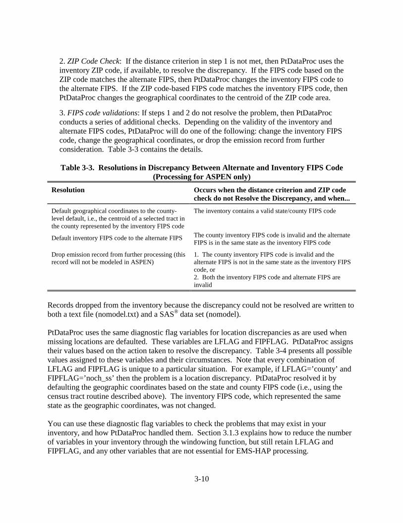
3-10
2. ZIP Code Check: If the distance criterion in step 1 is not met, then PtDataProc uses the inventory ZIP code, if available, to resolve the discrepancy. If the FIPS code based on the ZIP code matches the alternate FIPS, then PtDataProc changes the inventory FIPS code to the alternate FIPS. If the ZIP code-based FIPS code matches the inventory FIPS code, then PtDataProc changes the geographical coordinates to the centroid of the ZIP code area.
3. FIPS code validations: If steps 1 and 2 do not resolve the problem, then PtDataProc conducts a series of additional checks. Depending on the validity of the inventory and alternate FIPS codes, PtDataProc will do one of the following: change the inventory FIPS code, change the geographical coordinates, or drop the emission record from further consideration. Table 3-3 contains the details.
Table 3-3. Resolutions in Discrepancy Between Alternate and Inventory FIPS Code
(Processing for ASPEN only) Resolution Occurs when the distance criterion and ZIP code
check do not Resolve the Discrepancy, and when...
Default geographical coordinates to the county-level default, i.e., the centroid of a selected tract in the county represented by the inventory FIPS code
The inventory contains a valid state/county FIPS code
Default inventory FIPS code to the alternate FIPS The county inventory FIPS code is invalid and the alternate FIPS is in the same state as the inventory FIPS code
Drop emission record from further processing (this record will not be modeled in ASPEN)
1. The county inventory FIPS code is invalid and the alternate FIPS is not in the same state as the inventory FIPS code, or 2. Both the inventory FIPS code and alternate FIPS are invalid
Records dropped from the inventory because the discrepancy could not be resolved are written to both a text file (nomodel.txt) and a SAS® data set (nomodel). PtDataProc uses the same diagnostic flag variables for location discrepancies as are used when missing locations are defaulted. These variables are LFLAG and FIPFLAG. PtDataProc assigns their values based on the action taken to resolve the discrepancy. Table 3-4 presents all possible values assigned to these variables and their circumstances. Note that every combination of LFLAG and FIPFLAG is unique to a particular situation. For example, if LFLAG=’county’ and FIPFLAG=’noch_ss’ then the problem is a location discrepancy. PtDataProc resolved it by defaulting the geographic coordinates based on the state and county FIPS code (i.e., using the census tract routine described above). The inventory FIPS code, which represented the same state as the geographic coordinates, was not changed. You can use these diagnostic flag variables to check the problems that may exist in your inventory, and how PtDataProc handled them. Section 3.1.3 explains how to reduce the number of variables in your inventory through the windowing function, but still retain LFLAG and FIPFLAG, and any other variables that are not essential for EMS-HAP processing.

3-11
Table 3-4. Assignment of Diagnostic Flag Variables LFLAG and FIPFLAG
(Processing For ASPEN only)
Location Data Evaluation Values Assigned to Flag Variables
Geographic coordinates defaulted based on county (i.e., census tract routine) due to invalid coordinates (LLPROB has value of ‘missing’ or ‘bad_loc’)
LFLAG = ‘county’ AND FIPFLAG is not assigned a value
Geographic coordinates defaulted by ZIP code due to invalid coordinates (LLPROB has value of ‘missing’ or ‘bad_loc’) and the inventory FIPS code and ZIP code-based FIPS code agree
LFLAG = ‘zipcode’ AND FIPFLAG is not assigned a value
Geographic coordinates defaulted by ZIP code due to invalid coordinates (LLPROB has value of ‘missing’ or ‘bad_loc’) and inventory FIPS code is reassigned to the ZIP code-based FIPS code. Note: this happens when the inventory FIPS code is invalid and the state as determined by the inventory FIPS code is the same as the state determined by the ZIP code.
LFLAG = ‘zipcode’ AND FIPFLAG = ‘assigned’
Geographic coordinates defaulted based on county to resolve disagreement between inventory FIPS code and alternate FIPS (LLPROB does not have value of ‘missing’ or ‘bad_loc’)
LFLAG = ‘county’ AND FIPFLAG = ‘noch_ss’, when inventory FIPS code and alternate FIPS represent the same state; FIPFLAG = ‘noch_ds’, when inventory FIPS code and alternate FIPS represent different states
Geographic coordinates defaulted by ZIP code to resolve disagreement between inventory FIPS code and alternate FIPS (LLPROB variable does not have value of ‘missing’ or ‘bad_loc’)
LFLAG = ‘zipcode’ AND FIPFLAG = ‘noch_ss’, when inventory FIPS code and alternate FIPS represent the same state; FIPFLAG =‘noch_ds’, when inventory FIPS code and alternate FIPS represent different states
Inventory FIPS code disagrees with alternate FIPS, but the distance criterion is met so no change is made to either FIPS code or lat/lon. (This would likely occur when point source is near a state or county border.)
LFLAG is not assigned a value AND FIPFLAG = ‘noch_ss’, when inventory FIPS code and alternate FIPS represent the same state; FIPFLAG = ‘noch_ds’, when inventory FIPS code and alternate FIPS represent different states
Inventory FIPS code disagrees with alternate FIPS, and is reassigned to the ZIP code-based FIPS code
LFLAG is not assigned a value AND FIPFLAG = ‘ZIP_ss’, when inventory FIPS code and alternate FIPS represent the same state; FIPFLAG = ‘ZIP_ds’, when inventory FIPS code and alternate FIPS represent different states
Inventory FIPS code disagrees with alternate FIPS, and is reassigned to the alternate FIPS
LFLAG is not assigned a value AND FIPFLAG = ‘reloc_ss’, when inventory FIPS code and alternate FIPS represent the same state; FIPFLAG = ‘reloc_ds’, when inventory FIPS code and alternate FIPS represent different states
Discrepancy between Inventory FIPS code and alternate FIPS cannot be resolved
LFLAG is not assigned a value AND FIPFLAG = ‘no_model’

3-12
3.1.2 PtDataProc quality assures stack parameters; defaults if missing or out-of-range PtDataProc checks each record for valid stack parameters and provides defaults to missing or out-of-range data. PtDataProc determines if a non-missing stack parameter is out-of-range by comparing it to the minimum and maximum range values you provide in the batch file (see the “Valid Stack Parameter Ranges” section of Table 3-11 or 3-12 in Section 3.2.5). Because COPAX (Chapter 2) sets the stack parameters for allocated emissions to missing, PtDataProc will default stack parameters for these emission records. PtDataProc defaults missing allocated emission stack parameters the same way it defaults all other missing stack parameters as described below. Note that stack parameters are not used for ISCST3 volume sources or ISCST3 area sources (including allocated emissions processed using COPAX). To process these sources, you must include additional release parameters in your inventory (see Table 3-7 in Section 3.2.1 or, for allocated emissions, see Section 2.1.3). Nonetheless, PtDataProc will check and default point source stack parameters for these sources where missing or out-of-range. PtDataProc will not check or default the ISCST3 area source or volume source release parameters; thus, you must be careful when supplying this information to your inventory. You can choose several ways for PtDataProc to default missing or out-of-range stack parameters by providing the proper keywords in your batch file (see Section 3.2.3 for details). You can have PtDataProc assign default stack parameters using the 8-digit Source Classification Code (SCC)-based and/or 4-digit Standard Industrial Classification (SIC)-based defaults. If you choose either SCC-based or SIC-based defaults, PtDataProc uses ancillary SCC or SIC default files. If you choose both SCC-based and SIC-based defaults, and an inventory record can be matched to values in both default files, the program will use the SCC-based default over the SIC-based one. Some stack parameters may not be addressed by either of these methods (e.g., if an inventory record has no SCC nor SIC) or, you may choose not to use these options. In these cases, PtDataProc uses the following “global” defaulting routine: (1) If the stack parameters are missing, PtDataProc will default them to the global stack parameters you provide in the batch file (see Tables 3-10 or 11), (2) If the stack parameters are outside of the valid range you provide in the batch file, PtDataProc will use either the minimum or maximum range value as the default. The one exception to this global defaulting routine is for horizontal stacks or fugitives (EMRELPTY = ‘03' or ‘01'). If the stack parameters are missing or zero for these, PtDataProc uses the following defaults: stack height of 5 meters, stack diameter of 1 meter, stack temperature of 295 K and stack velocity of 0.5 meters/second. When processing for ISCST3, these stack parameters are not used for horizontal stacks or fugitives, because in the EMS-HAP program PtFinal_ISCST3 converts these sources to ISCST3 volume sources (see Section 8.1.2) and volume source release parameters are used. PtDataProc sets diagnostic flag variables, for each defaulted stack parameter (HTFLAG, DIAFLAG, VELFLAG, and TEMPFLAG), to explain why and how each was defaulted; these

3-13
are summarized in Table 3-5. Section 3.1.3 explains how to reduce the number of variables in your inventory through the windowing function, but still retain these diagnostic variables, and any other variables that are not essential for EMS-HAP processing.
Table 3-5. Assignment of Stack Parameter Defaulting Diagnostic Flag Variables
Default Method
Evaluation of Invalid Stack Parameter
Default Value Assigned
Value Assigned to Diagnostic Flag Variables HTFLAG, DIAFLAG, VELFLAG, and TEMPFLAG
SCC
Parameter is not missing, but is outside of valid parameter range
SCC-based default
Concatenation of the value of DEFFLAG variable* from the SCC default file and ‘out’
Parameter is missing SCC-based default
Concatenation of the value of DEFFLAG variable* from the SCC default file and ‘miss’
SIC
Parameter is not missing, but is outside of valid parameter range
SIC-based default
Concatenation of the value of DEFFLAG variable* from the SIC default file and ‘out’
Parameter is missing SIC-based default
Concatenation of the value of DEFFLAG variable* from the SIC default file and ‘miss’
Neither SCC nor SIC
Parameter is missing Global default ‘default’
Parameter is not missing, but is less than the minimum range value
Minimum range value
‘rangelow’
Parameter is not missing, but is greater than the maximum range value
Maximum range value
‘rangehi’
* the DEFFLAG variable indicates the method used to obtain the default value. See description in SCCDEFLT and SICDEFLT file formats provided in Appendix A.
3.1.3 PtDataProc removes inventory variables and records not necessary for further processing (inventory windowing)
Because point source inventories can be very large, it is useful for further processing of the data through EMS-HAP to reduce the size of the inventory file as much as possible. The PtDataProc program allows you to do this in two ways: (1) by removing nonessential variables from your inventory and (2) by removing nonessential records from your inventory.

3-14
Note that PtDataProc outputs both the windowed and non-windowed inventory. The non-windowed inventory, named by keyword OUTSAS, contains a complete list of variables, including non-essential variables included in your input inventory and non-essential flag variables added by PtDataProc such as LFLAG, FIPFLAG, LLPROB and DEFLTRCT. You would use the windowed inventory for input into PtModelProc; the non-windowed inventory could be used for further analysis of the inventory. Removal of Nonessential Variables To window the inventory, you can choose to have PtDataProc remove all variables except for those required for further processing within EMS-HAP. To do this, set the value of the DOSETVAR keyword to 1 in your batch file (see Table 3-9 in Section 3.2.3). You also have the option of providing PtDataProc with a list of additional variables (e.g., LLPROB, LFLAG, FIPFLAG) to be retained. When processing data for ISCST3, PtDataProc checks for the existence of the optional building dimension variables and the release parameters required to process ISCST3 area sources and volume sources (see Table 3-7). If these variables are present, PtDataProc will automatically retain them in the output inventory. To retain additional variables, set the DOSETVAR and USELIST keywords in your batch file to 1 (one), and provide a list of nonessential variables in an ancillary text file (see the VARLIST keyword in Table 3-8). Removal of Nonessential Records Another way to window the inventory is that you can choose to have PtDataProc remove all records that have geographic coordinates or that have zero emissions. To do this, assign a value of “1” to the DOWINDOW keyword in your batch file. Note that if you choose to have PtDataProc perform the location data quality assurance function, windowing the inventory to remove records without location coordinate data would not be necessary, because these records would have already been removed. You would still, however, need to perform the windowing function if you want to remove records with zero emissions. 3.2 How do I run PtDataProc? 3.2.1 Prepare your point source inventory for input into PtDataProc The point source inventory you use for input into PtDataProc can be your initial point source inventory, or, if you choose to process allocated emissions as point source emissions, it can be the output from COPAX (see Chapter 2). When processing data for ISCST3, please note the following: $ You have the option of including ISCST3 volume sources and ISCST3 area sources in your
point source inventory. An ISCST3 volume source is used to model emission releases from various industrial sources, such as building roof monitors, multiple vents, and conveyor belts. An ISCST3 area source is used to model low level or ground level emission releases with no

3-15
plume rise, such as storage piles, slag dumps, lagoons, landfills, or airports. An ISCST3 area source can also be used to model onroad mobile emissions by assigning the emissions to rectangular road segments.
$ You can include building parameters in your point source inventory. See the last three bullets below on how to include these when processing for ISCST3. Your input point source inventory must meet the following requirements: C It must be in SAS® file format. C To complete all point source programs, your data must contain the variables in Table 3-6
with units and values as provided. Additional variables can be present, and will be included in the output SAS® file. However, you can choose to create an output file with only those variables needed in subsequent EMS-HAP processing programs by choosing the windowing function which was discussed in Section 3.1.3.
C All data records must be uniquely identifiable by using the combination of the site ID (SITE_ID), pollutant code (CAS), and emission release point ID (EMRELPID).
C All stack parameters within a group of records identified by the site ID (SITE_ID), and emission release point ID (EMRELPID) must be the same.
C When processing data for ISCST3, if you choose to model some of your sources as ISCST3 volume sources (as discussed earlier in this section), your inventory must include the ISCST3 source type variable ISCTYPE (which must be ‘iscvolume’), and release parameter variables VOLHGT, SIGMAX, and SIGMAY as listed in Table 3-7.
C When processing data for ISCST3, if you choose to model some of your sources as ISCST3 area sources (as discussed earlier in this section), your inventory must include the ISCST3 source type variable ISCTYPE (which must be ‘iscarea’), and release parameter variables ARELHGT and AXLEN as listed in Table 3-7. Release parameter variables AYLEN, AANGLE, and AINPLUM are optional. The locational coordinates in your inventory should represent the center of the area source.
C When processing data for ISCST3, if you choose to include building parameters in your point source inventory, then building height must be specified by a variable called BLDH, and building width by BLDW, and they both must be expressed in meters.

3-16
Table 3-6. Variables Required for PtDataProc Input Point Source Inventory SAS® File
Variables used by PtDataProc are in bold; other variables listed are used by subsequent point source processing programs. Variable Name Data Description
(Required units or values are in parentheses)Type*
CAS unique pollutant code A10
CNTL_EFF baseline control efficiency, expressed as a percentage N
EMIS pollutant emissions value (tons/year) N
EMRELPID code identifying a unique emission point within a site A50
EMRELPTY physical configuration code of release point (01=fugitive; 02=vertical stack; 03=horizontal stack, 04=goose neck, 05=vertical with rain cap, 06=downward-facing vent, 99=missing, AP=allocated to point during COPAX –e.g., aircraft)
A4
FIPS 5-digit FIPS code (state and county combined) A5
MACT MACT code; if variable name is MACTCODE, PtDataProc will rename as MACT A7
SCC EPA source category code identifying the process A10
SIC Standard Industrial Classification (SIC) code for the site A4
SITE_ID code identifying a unique site A25
SRC_TYPE description of the emission source at the site (i.e., ‘nonroad’ for allocated nonroad or combined onroad and nonroad mobile county-level emissions; ‘area’ for allocated non-point county-level emissions). If you choose to define source groups by this variable as explained in 7.1.1 or 8.1.1, or run PtGrowCntl (Chapter 6) then it must have the value of ‘major’ or ‘area’ for non-allocated emissions.
A15
STACKDIA diameter of stack (meters) N
STACKHT height of stack (meters) N
STACKVEL velocity of exhaust gas stream (meters per second) N
STKTEMP temperature of exhaust gas stream (Kelvin) N
UTM_Z universal transverse mercator (UTM) zone N
X longitude (decimal degrees or degrees, minutes, seconds with no separating characters) or UTM easting (meters or kilometers)
N
XY_TYPE type of coordinate system used (LAT/LON or UTM) A7
Y latitude (decimal degrees or degrees, minutes, seconds with no separating characters) or UTM northing (meters or kilometers)
N
ZIP_CODE ZIP code of site A12 * Ax = character string of length x, N = numeric

3-17
Table 3-7. Additional Variables for PtDataProc Input Point Source Inventory SAS® File When Processing ISCST3 Area or Volume Sources
Required variables are in bold. Variable Name Data Description
(Required units or values are in parentheses) Type*
AANGLE orientation angle of rectangle for ISCST3 area sources (degrees from North) N
AINPLUM initial vertical dimension of plume for ISCST3 area source (meters) N
ARELHGT release height above ground for ISCST3 area sources (meters) N
AXLEN length of X side of rectangle for ISCST3 area sources (meters) N
AYLEN length of Y side of rectangle for ISCST3 area sources (meters) N
ISCTYPE ISCST3 source type (iscvolume or iscarea) A9
SIGMAX initial lateral dimension of volume source (meters) N
SIGMAZ initial vertical dimension of volume source (meters) N
VOLHGT release height above ground for volume source (meters) N * Ax = character string of length x, N = numeric
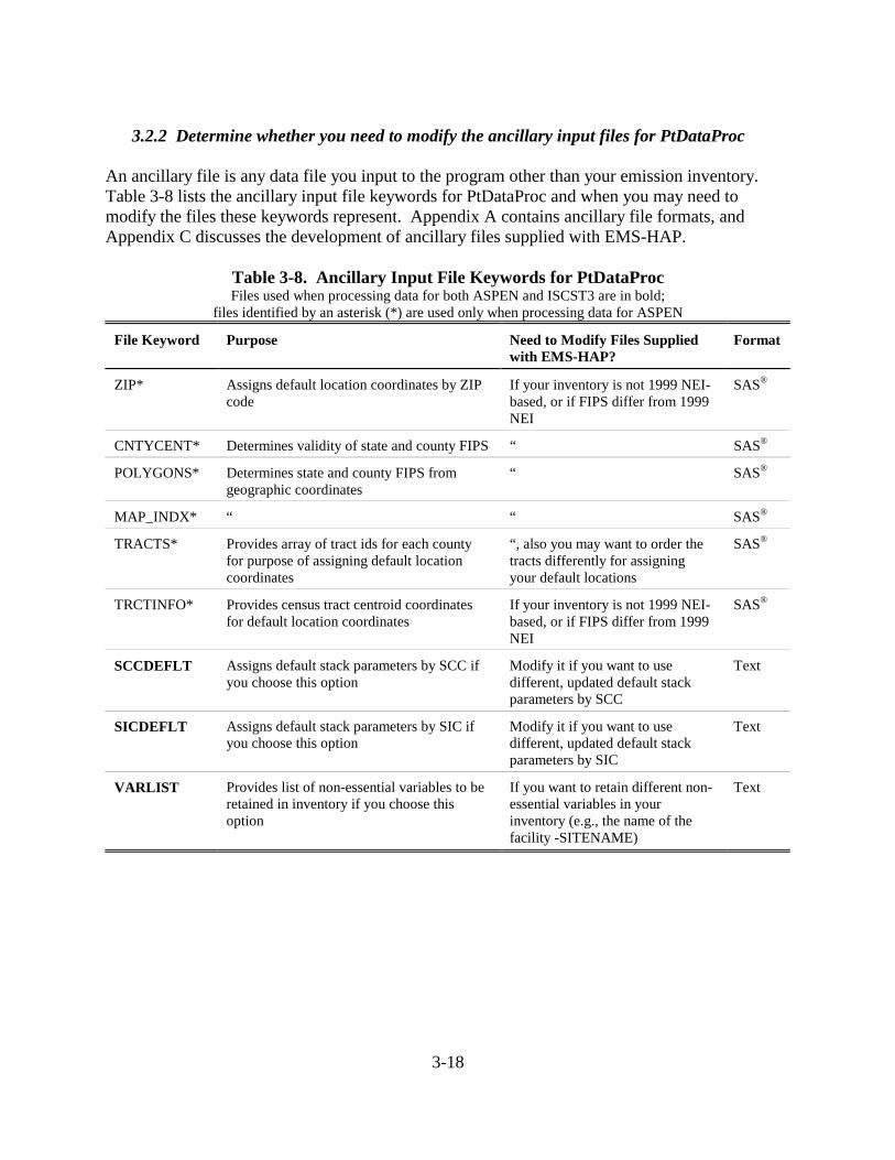
3-18
3.2.2 Determine whether you need to modify the ancillary input files for PtDataProc An ancillary file is any data file you input to the program other than your emission inventory. Table 3-8 lists the ancillary input file keywords for PtDataProc and when you may need to modify the files these keywords represent. Appendix A contains ancillary file formats, and Appendix C discusses the development of ancillary files supplied with EMS-HAP.
Table 3-8. Ancillary Input File Keywords for PtDataProc Files used when processing data for both ASPEN and ISCST3 are in bold;
files identified by an asterisk (*) are used only when processing data for ASPEN File Keyword Purpose Need to Modify Files Supplied
with EMS-HAP? Format
ZIP* Assigns default location coordinates by ZIP code
If your inventory is not 1999 NEI-based, or if FIPS differ from 1999 NEI
SAS®
CNTYCENT* Determines validity of state and county FIPS “ SAS®
POLYGONS* Determines state and county FIPS from geographic coordinates
“ SAS®
MAP_INDX* “ “ SAS®
TRACTS* Provides array of tract ids for each county for purpose of assigning default location coordinates
“, also you may want to order the tracts differently for assigning your default locations
SAS®
TRCTINFO* Provides census tract centroid coordinates for default location coordinates
If your inventory is not 1999 NEI-based, or if FIPS differ from 1999 NEI
SAS®
SCCDEFLT Assigns default stack parameters by SCC if you choose this option
Modify it if you want to use different, updated default stack parameters by SCC
Text
SICDEFLT Assigns default stack parameters by SIC if you choose this option
Modify it if you want to use different, updated default stack parameters by SIC
Text
VARLIST Provides list of non-essential variables to be retained in inventory if you choose this option
If you want to retain different non-essential variables in your inventory (e.g., the name of the facility -SITENAME)
Text

3-19
3.2.3 Prepare your batch file The batch file serves two purposes: (1) allows you to pass “keywords” such as file names and locations, program options, and run identifiers to the program, and (2) sets up the execute statement for the program. Sample batch files for PtDataProc for ASPEN and ISCST3 emissions processing are shown in Figures B-4 and B-5, respectively, of Appendix B. The best way to prepare your batch file is to use one of the samples we provide and modify it to fit your needs. Specify your keywords Table 3-9 shows you how to specify keywords to select which functions you want PtDataProc to perform. For example, if you’ve already calculated your appropriate location coordinates and quality assured them, you may choose not to use this function. For this situation, set the keyword “DOLOCATE” to zero.
Table 3-9. Keywords for Selecting PtDataProc Functions
PtDataProc Function Keyword (values provided cause function to be performed)
Process data for ASPEN model MODEL = ASPEN
Process data for ISCST3 model MODEL = ISC
Quality assurance of location data DOLOCATE = 1
Quality assurance of stack parameters and defaulting of allocated (by COPAX) point source. emission stack parameters
DOSTACK=1
Use SCC based defaults; use global defaults or range defaults if parameters are still missing or out-of-range after SCC default process
DOSCCDEF = 1; DOSICDEF = 0
Use SIC based defaults; use global defaults or range defaults if parameters are still missing or out-of-range after SIC default process
DOSCCDEF = 0; DOSICDEF = 1
Use both SIC and SCC based defaults; use global defaults or range defaults if parameters are still missing or out-of-range (Note: when single record can be defaulted by both SIC and SCC-based defaults, PtDataProc will use the SCC default)
DOSCCDEF = 1; DOSICDEF = 1
Use only global defaults (range defaults if parameters are out of range) DOSICDEF = 0; DOSCCDEF = 0
Window Inventory to reduce variable list DOSETVAR = 1
Specify additional variables to retain on output inventory file USELIST = 1
Don’t retain any non-essential variables on output inventory file USELIST = 0
Window Inventory to exclude zero emissions and non-located records DOWINDOW=1 A complete list of keywords required in the batch file for the ASPEN model is presented in Table 3-10. Keywords required for the ISCST3 model are in Table 3-11. PtDataProc does not

3-20
require a value for every keyword for all execution scenarios. For example, the ZIP, CNTYCENT, MAP_INDX, POLYGONS, TRACTS, and TRACTINFO, keywords are not used for ASPEN processing if DOLOCATE is set to zero (0). However, it is easier to create PtDataProc batch files for different execution scenarios if all keywords are at least present in an existing batch file. Note the sections called “Valid Stack Parameter Ranges” and “Global Stack Parameters” are used to process data for both ASPEN and ISCST3. You supply the values for stack parameter ranges used to determine if a stack parameter is valid. PtDataProc will use the upper or lower bounds of the range as a “range default” if parameters are not defaulted using SCC and/or SIC based defaults. You also supply values for global default stack parameters for missing stack parameters not defaulted by the other methods.
Table 3-10. Keywords in the PtDataProc Batch File when Processing Data for ASPEN
Keyword Description of Value Input Inventory Files IN_DATA Name of directory containing the input inventory SAS® file INSAS Input inventory SAS® file name, prefix of file name only Ancillary Files REFFILE Name of directory containing ancillary files that are SAS® files REFTEXT Name of directory containing ancillary files that text files ZIP ZIP code to FIPS and lat/lon cross-reference SAS® file, prefix only CNTYCENT County FIPS to county centroid location SAS® file, prefix only MAP_INDX SAS® index file that contains information on the POLYGONS ancillary file (see next row),
prefix only POLYGONS Used for state and county FIPS QA, SAS® file, prefix only TRACTS Tract array containing a list of tracts for each County FIPS SAS® file, prefix only TRCTINFO Census tracts to state and county FIPS code, tract centroid, and tract radius correspondence
SAS® file, prefix only SCCDEFLT SCC to default stack parameters correspondence text file, prefix only SICDEFLT SIC to default stack parameters correspondence text file, prefix only VARLIST File containing user’s choice of additional, nonessential variables to be retained in inventory
output file, prefix only Program Options (also see Table 3-9) MODEL ASPEN= process data for ASPEN model DOLOCATE 1= quality assure location data; 0= don’t quality assure them DOSTACK 1= quality assure stack parameters; 0= don’t quality assure them. DOSCCDEF 1= assign default stack parameters by SCC; 0= don’t assign them by SCC DOSICDEF 1= assign default stack parameters by SIC; 0= don’t assign them by SIC DOSETVAR 1= retain variables required for further processing and only those non-essential variables
specified by you, based on value of USELIST and VARLIST 0= retain all variables

Table 3-10. Keywords in the PtDataProc Batch File when Processing Data for ASPEN (continued)
3-21
Keyword Description of Value USELIST 1= use ancillary file (keyword VARLIST) to provide additional non-essential variables to
retain in inventory 0= don’t retain any non-essential variables from the inventory
DOWINDOW 1= remove all records with zero emissions values or records without latitude and longitude values 0= don’t remove records with zero emissions or without latitude and longitude values (note that values without latitude and longitude values will still be removed if you perform the data quality assurance of location data function)
Valid Stack Parameter Ranges DLOWHT Minimum range value for valid stack height (in meters) DHIHT Maximum range value for valid stack height (in meters) DLOWDIA Minimum range value for valid stack diameter (in meters) DHIDIA Maximum range value for valid stack diameter (in meters) DLOWVEL Minimum range value for valid stack velocity (in meters/second) DHIVEL Maximum range value for valid stack velocity (in meters/second) DLOWTEMP Minimum range value for valid stack temperature (in Kelvin) DHITEMP Maximum range value for valid stack temperature (in Kelvin) Global Default Stack Parameters DFLTHT Default stack height (in meters) DFLTDIA Default stack diameter (in meters) DFLTVEL Default stack exit gas velocity (in meters/second) DFLTTEMP Default stack exit gas temperature (in Kelvin) Output files OUTDATA Name of directory containing output inventory SAS® file OUTTEXT Name of directory containing text file of records without latitude/longitude data OUTSAS Output inventory SAS® file name (contains all variables and records), prefix only FINAL Output inventory SAS® file name after windowing, prefix only NOLOCATE Output data SAS® file name containing records without coordinates, prefix only ZEROEMIS Output data SAS® file name containing records with zero emissions values, prefix only

3-22
Table 3-11. Keywords in the PtDataProc Batch File when Processing Data for ISCST3
Keyword Description of Value Input Inventory Files IN_DATA Name of directory containing the input inventory SAS® file INSAS Input inventory SAS® file name, prefix of file name only Ancillary Files REFTEXT Name of directory containing the ancillary files SCCDEFLT SCC to default stack parameters correspondence text file, prefix only SICDEFLT SIC to default stack parameters correspondence text file, prefix only VARLIST File containing user’s choice of additional, nonessential variables to be retained in inventory
output file, prefix only Program Options (also see Table 3-9) MODEL ISC= process data for ISCST3 model DOLOCATE 1= quality assure location data; 0= don’t quality assure them DOSTACK 1= quality assure stack parameters; 0= don’t quality assure them. DOSCCDEF 1= assign default stack parameters by SCC; 0= don’t assign them by SCC DOSICDEF 1= assign default stack parameters by SIC; 0=don’t assign them by SIC DOSETVAR 1= retain variables required for further processing and only those non-essential variables
specified by you, based on the value of USELIST and VARLIST 0= retain all variables
USELIST 1= use ancillary file (keyword VARLIST) to provide additional non-essential variables to retain in inventory 0= don’t retain any non-essential variables from the inventory
DOWINDOW 1= remove all records with zero emissions values or records without latitude and longitude values 0= don’t remove records with zero emissions or without latitude and longitude values (note that values without latitude and longitude values will still be removed if you perform the data quality assurance of location data function)
Valid Stack Parameter Ranges DLOWHT Minimum range value for valid stack height (in meters) DHIHT Maximum range value for valid stack height (in meters) DLOWDIA Minimum range value for valid stack diameter (in meters) DHIDIA Maximum range value for valid stack diameter (in meters) DLOWVEL Minimum range value for valid stack velocity (in meters/second) DHIVEL Maximum range value for valid stack velocity (in meters/second) DLOWTEMP Minimum range value for valid stack temperature (in Kelvin) DHITEMP Maximum range value for valid stack temperature (in Kelvin) Global Default Stack Parameters DFLTHT Default stack height (in meters) DFLTDIA Default stack diameter (in meters) DFLTVEL Default stack exit gas velocity (in meters/second) DFLTTEMP Default stack exit gas temperature (in Kelvin)

Table 3-11. Keywords in the PtDataProc Batch File when Processing Data for ISCST3 (continued)
3-23
Keyword Description of Value Additional Input Data REF_ZONE UTM zone for ISCST3 model domain Output files OUTDATA Name of directory containing output inventory SAS® file OUTTEXT Name of directory containing text file of records without geographic coordinates OUTSAS Output inventory SAS® file name (contains all variables and records), prefix only FINAL Output inventory SAS® file name after windowing NOLOCATE Output data SAS® file name containing records without coordinates, prefix only ZEROEMIS Output data SAS® file name containing records with zero emissions values, prefix only
Prepare the execute statement The last line in the batch file runs the PtDataProc program. In the sample batch files provided in Figures B-4 and B-5 in Appendix B, you will see a line preceding the run line that creates a copy of the PtDataProc code having a unique name. It is this version of the program that is then executed in the last line. If you do this, the log and list files created by this run can be identified by this unique name. If you don’t do this and run the program under a general name, every run of PtDataProc will create a log and a list file that replace any existing files of the same name. You may find that you need to define a special area on your hard disk to use as workspace when running PtDataProc. In the sample batch file, a work directory is defined on the last line following the execution of PtDataProc. The directory you reference here must be created prior to running the program. For example, the statement: ‘sas ptdataproc_061600.sas -work /data/work1/dyl/’ assigns a SAS® work directory in the “/data/work1/dyl” directory. 3.2.4 Execute PtDataProc There are two ways to execute the batch file. One way is to type ‘source’ and then the batch file name. Alternatively, first set the permission on the file to ‘execute.’ You do this by using the UNIX chmod command and adding the execute permission to yourself, as the owner of the file, to anyone in your user group, and/or to anyone on the system. For example, ‘chmod u+x PtDataProc.bat’ gives you permission to execute the batch file. Refer to your UNIX manual for setting other permissions. After you have set the file permission, you can execute the batch file by typing the file name on the command line, for example, ‘PtDataProc.bat’.

3-24
3.3 How do I know my run of PtDataProc was successful? 3.3.1 Check your SAS® log file You need to review the output log file to check for errors or other flags indicating incorrect processing. This review should include searching the log files for occurrences of the strings “ERROR”, “WARNING”, “not found”, and “uninitialized”. These can indicate problems with input files or other errors. You can also look at the number of records in the input inventory file and compare it to the number of records in the output inventory file. The number of records shouldn’t change unless PtDataProc removed records during the quality assurance of the location data or during the windowing of the inventory. If so, you can determine the number of dropped records by summing the records written to the PtDataProc output files containing the records which have been dropped from the inventory (files “nolocate” and “nomodel”) and the SAS® file containing the records with zero emissions (file named by keyword ZEROEMIS). 3.3.2 Check your SAS® list file The list file created when PtDataProc is executed contains information to assist in quality assurance. This file can contain the information listed below. The contents of the list file from a specific run of PtDataProc depend on which functions you choose to have PtDataProc perform. C First 100 sites* requiring location defaulting due to missing or invalid location data (when
processing data for ASPEN only) C First 100 sites* dropped from the inventory because a default location could not be
determined; emission total from all records dropped from inventory (when processing data for ASPEN only)
C First 100 sites* dropped from the inventory because the disagreement between the location and FIPS of the site could not be resolved; emission total from all records dropped from inventory (when processing data for ASPEN only)
C Pollutant and state-level emission totals and record counts after all location defaulting is complete (when processing data for ASPEN only)
C First 100 sites* with out-of-range stack parameters; emission total from all records with out-of-range stack parameters
C Pollutant and state-level emission totals and record counts after defaulting stack parameters * You can analyze the output inventory and additional QA files (Section 3.3.3) to get a complete list of sites with the above-stated problems. We chose 100 of them to be printed out in the list file arbitrarily.

3-25
3.3.3 Check other output files from PtDataProc You should check for the existence of the output inventory file named by keyword FINAL if you chose to window the inventory, or by keyword OUTSAS if you didn’t. While either of these two files can serve as the input to PtModelProc, you’ll likely want to use the file you reduced through the window function (named by keyword FINAL) to minimize the disk space use. PtDataProc also creates SAS® and ASCII formatted output files, shown in Table 3-12, containing information on the location and stack parameters were defaulted or dropped from the inventory.
Table 3-12. Additional QA Files Created by PtDataProc*
QA output files
Function: Quality assurance of location data when processing data for ISCST3
missing all records found to have missing location data; these records are dropped from the inventory
Function: Quality assurance of location data when processing data for ASPEN
dfltloc all records where location was defaulted because of missing or invalid location data
nolocate.txt, nolocate
all records dropped from inventory because a default location could not be determined
nomodel.txt, nomodel
all records dropped from inventory because discrepancy between location and county FIPS could not be resolved
Function: Quality assurance of stack parameters
stkcheck all records where stack parameters are outside a normally anticipated range of values you supply in the “Valid Stack Parameter Ranges” section of Table 3-10 or 3-11
Function: Window inventory to exclude nonzero emissions and unallocated sites
file named by keyword ZEROEMIS
all records dropped from the inventory where emission values are zero
file named by keyword NOLOCATE
all records dropped from inventory because either latitude and/or longitude are missing (Note: if you chose to quality assure the location data, then this file should be empty)
* Note, these files are output only if they contain records; that is, if no records have missing location data, the QA output file “missing” is not written.

3-26
This page intentionally blank

4-1
CHAPTER 4
Point Source Processing The Model-Specific Program (PtModelProc)
The flow charts below (Figure 4-1) show how PtModelProc fits into EMS-HAP’s point source processing for the ASPEN and ISCST3 models. The point source inventory you input to PtModelProc is the output from PtDataProc (Chapter 3). You use the output inventory from PtModelProc as the input to PtTemporal (Chapter 5).
Figure 4-1. Overview of PtModelProc within EMS-HAP Point Source Processing
PtDataProc
PtModelProc
PtTemporal
PtGrowCntl
PtFinal_ASPEN
OR
Point source emissions
ASPEN point source emission files
PtFinal_ISCST3
ISCST3 SO pathway of run stream section for
ISCST3 point, volume and area sources
Flowchart for ASPEN Processing Flowchart for ISCST3 Processing
Point source emissions
ORPtGrowCntl
PtTemporal
PtDataProc
PtModelProc
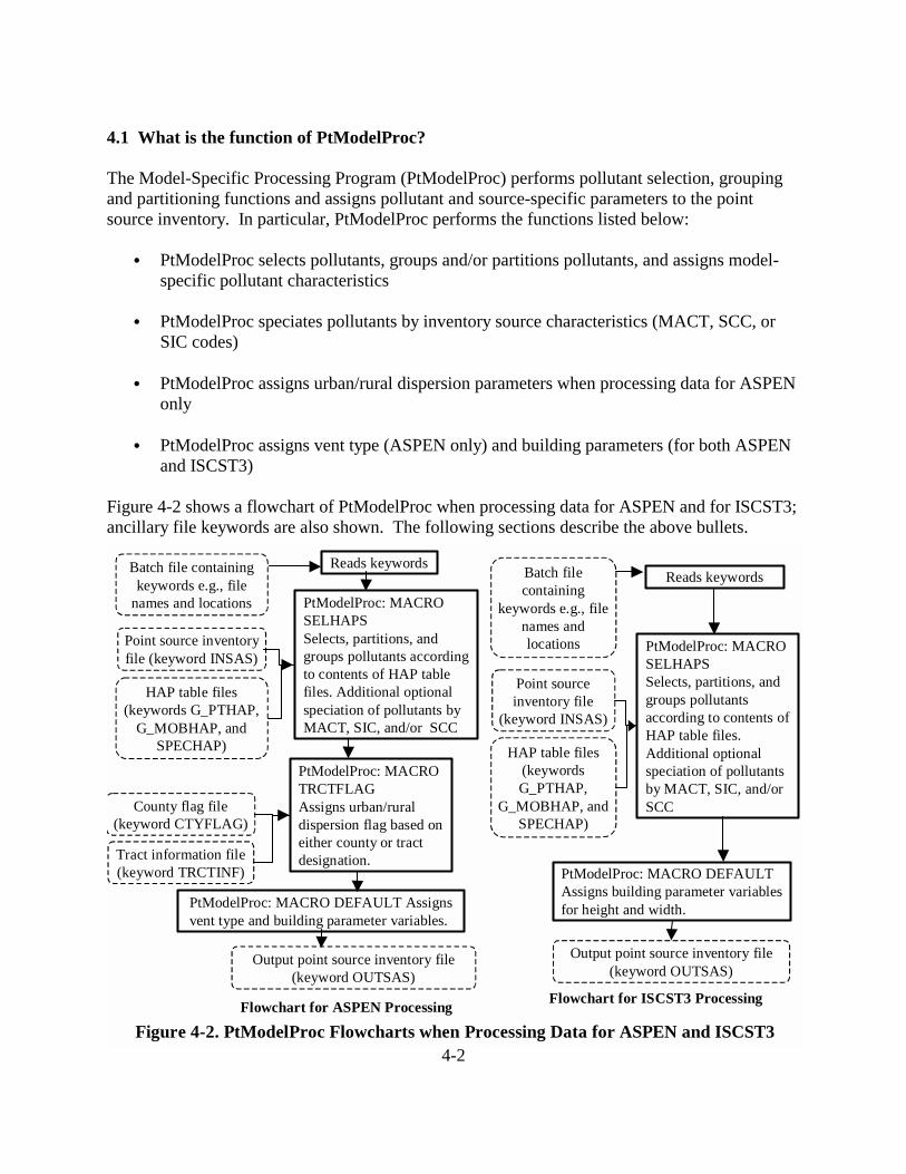
4-2
4.1 What is the function of PtModelProc? The Model-Specific Processing Program (PtModelProc) performs pollutant selection, grouping and partitioning functions and assigns pollutant and source-specific parameters to the point source inventory. In particular, PtModelProc performs the functions listed below:
C PtModelProc selects pollutants, groups and/or partitions pollutants, and assigns model-specific pollutant characteristics
C PtModelProc speciates pollutants by inventory source characteristics (MACT, SCC, or
SIC codes) C PtModelProc assigns urban/rural dispersion parameters when processing data for ASPEN
only C PtModelProc assigns vent type (ASPEN only) and building parameters (for both ASPEN
and ISCST3) Figure 4-2 shows a flowchart of PtModelProc when processing data for ASPEN and for ISCST3; ancillary file keywords are also shown. The following sections describe the above bullets.
Figure 4-2. PtModelProc Flowcharts when Processing Data for ASPEN and ISCST3
Output point source inventory file (keyword OUTSAS)
PtModelProc: MACRO DEFAULT Assigns vent type and building parameter variables.
Reads keywords
PtModelProc: MACRO SELHAPS Selects, partitions, and groups pollutants according to contents of HAP table files. Additional optional speciation of pollutants by MACT, SIC, and/or SCC
PtModelProc: MACRO TRCTFLAG Assigns urban/rural dispersion flag based on either county or tract designation.
County flag file (keyword CTYFLAG)
Tract information file (keyword TRCTINF)
Flowchart for ASPEN Processing
PtModelProc: MACRO DEFAULT Assigns building parameter variables for height and width.
Output point source inventory file (keyword OUTSAS)
Flowchart for ISCST3 Processing
Batch file containing
keywords e.g., file names and locations PtModelProc: MACRO
SELHAPS Selects, partitions, and groups pollutants according to contents of HAP table files. Additional optional speciation of pollutants by MACT, SIC, and/or SCC
Point source inventory file
(keyword INSAS)
HAP table files (keywords G_PTHAP,
G_MOBHAP, and SPECHAP)
Reads keywords
Point source inventory file (keyword INSAS)
HAP table files (keywords G_PTHAP,
G_MOBHAP, and SPECHAP)
Batch file containing keywords e.g., file
names and locations

4-3
4.1.1 PtModelProc selects pollutants, groups and/or partitions pollutants, and assigns model-specific pollutant characteristics
PtModelProc reads the point source inventory and selects, partitions, and/or groups pollutants to be modeled by either ASPEN or ISCST3. It also assigns the pollutant characteristics of “reactivity class” or “particulate size class” (variable REACT) that the ASPEN model uses to control reactive decay and deposition. Note that ISCST3 doesn’t use the reactivity/particulate class assignments. ISCST3 includes algorithms to model pollutant and source-specific gravitational settling and removal by wet and dry deposition; the variables required for these algorithms are assigned in PtFinal_ISCST3 (see Section 8.1.3). You control these functions through ancillary files you input to PtModelProc that we refer to as “general HAP tables”. PtModelProc’s use of the general HAP table is described in great detail in Section 4.2.3, where we discuss how you can modify one for your particular modeling application. Refer to that section for the details on the following items for which PtModelProc uses the general HAP table: C Subset the inventory to include only those pollutants you’ve chosen to model (KEEP variable
in Table 4-7); C Group multiple inventory species into a single pollutant category (Table 4-9); C Partition inventory species into multiple pollutant categories with different reactivity or
particulate size classes, e.g., apportion lead chromate to: 1) lead compounds, fine particulate; 2) lead compounds, coarse particulate; 3) chromium compounds, fine particulate and 4) chromium compounds, coarse particulate (Table 4-9);
C Assign a reactivity class to each gaseous pollutant and a particulate size class to each particulate pollutant (REACT variable in Table 4-7). Note that when processing for ISCST3, PtModelProc assigns this variable, but it is not used;
C Apply a mass adjustment factor (FACTOR variable in Table 4-7 and Table 4-10) to the emissions of an inventory species to partition it among multiple pollutant categories, account for a particular portion of it (e.g., the lead portion of lead sulfate), or adjust its potency to determine a toxics or reactivity equivalency;
C Assign the resulting pollutant or pollutant category to be modeled a unique HAP code (NTI_HAP variable in Table 4-7) used for inventory projections in PtGrowCntl, a unique pollutant code (SAROAD variable in Table 4-7) and a description (variable SAROADDC in Table 4-7).
PtModelProc uses two general HAP table files in a single run: one named by keyword G_MOBHAP, and the other named by keyword G_PTHAP. G_MOBHAP is used for the allocated nonroad mobile (e.g., aircraft) emissions, which you obtained by running COPAX. G_PTHAP is used for stationary sources, including the sources extracted and allocated from the county-level non-point inventory and all non-allocated point sources. PtModelProc uses the inventory variable SRC_TYPE (the source type) to determine which general HAP table to apply to each inventory record. All allocated nonroad (e.g., aircraft) emissions have SRC_TYPE = “nonroad” (this was assigned in COPAX, see section 2.1.2); these sources use G_MOBHAP.

4-4
PtModelProc’s utilization of two different general HAP tables enables you to assign different pollutant characteristics (e.g., different particulate size classes for the particulate pollutants) to the allocated nonroad (i.e., aircraft) emission sources when you run these sources together with the stationary-based point sources through the point source processing programs. PtModelProc may not need to use both G_PTHAP and G_MOBHAP for a single run. In the situation where no sources have a SRC_TYPE of “nonroad” (which happens when the county-level inventory fed into COPAX was non-point, or no allocated emissions from COPAX are appended with the point source inventory), PtModelProc will only use G_PTHAP. PtModelProc still reads the keyword G_MOBHAP; however, because nonroad mobile sources are not in the inventory in this case, PtModelProc will not attempt to process emissions or the nonroad mobile HAP table. The general HAP tables apply uniformly across all processes and all pollutants (except that the nonroad sources can use a different general HAP table as described above). As a result, with the general HAP table, all nonroad sources would undergo the same partioning of metal compounds (e.g., chromium into a particular percentage of coarse and fine) regardless of the specific nonroad category (aircraft versus airport support vehicles). PtModelProc allows process-level speciation through the use of the specific HAP table (discussed in the next section). You can use this feature to speciate chromium into hexavalent and non-hexavalent (i.e., trivalent) forms by the particular industry type or process (e.g., chromium electroplating). 4.1.2 PtModelProc speciates pollutants by inventory source characteristics (MACT, SCC,
or SIC codes) In addition to the two general HAP tables, an optional “specific HAP table” (ancillary file SPECHAP) can be applied. PtModelProc uses SPECHAP for speciating pollutants that have already been partitioned or grouped by the general HAP tables. PtModelProc speciates the pollutants (or pollutant groups) from the general HAP table into the desired species for modeling based on the inventory pollutant (variable CAS) and either the MACT, SCC or SIC codes, which characterize the type of source. We incorporated this function in EMS-HAP to allow chromium compounds that are inventoried as unspeciated groups (e.g., “chromium and compounds”) to be speciated into hexavalent and non-hexavalent forms based on the type of source. PtModelProc applies the factors in the SPECHAP file after it applies the general HAP table factors. In the case of chromium, for example, SPECHAP takes emissions from “Chromium and Compounds” (CAS #136) from: 1) chromium compounds, fine particulate; and 2) chromium compounds, coarse particulate, and speciates them to: 1) hexavalent chromium compounds, fine particulate; 2) hexavalent chromium compounds, coarse particulate; 3) non-hexavalent chromium compounds, fine particulate; and 4) non-hexavalent chromium compounds, coarse particulate. When more than one speciation factor in the SPECHAP file could apply to a particular inventory record, PtModelProc uses the hierarchy shown in Table 4-1.

4-5
Table 4-1. Hierarchy for Applying Speciation Information
Order of Precedence MACT SCC SIC CAS1 (most specific information, supercedes all others) X X 2 X X 3 X X 4 (least specific information -- Default) X You must include a “CAS-level” default (last row in Table 4-1) for each unique CAS in the SPECHAP file. PtModelProc will apply this default to any record in the inventory (with the appropriate CAS) in which the MACT, SCC, or SCC-level speciation factors in SPECHAP do not apply. For example, if a particular source of chromium compounds (CAS=136) has no MACT or SCC code and has an SIC code that is not present in the SPECHAP file, then PtModelProc will apply the default speciation factor for CAS=136 listed in the SPECHAP file. This will allow that source to be speciated. Section 4.2.4 contains instructions on how to modify a specific HAP table to meet your needs. Appendix C discusses how we developed the SPECHAP file supplied with EMS-HAP.
4.1.3 PtModelProc assigns urban/rural dispersion parameters when processing data for ASPEN only
The dispersion algorithm in the ASPEN model uses different dispersion parameters and deposition rates for urban and rural sources to account for the effect of surface characteristics (e.g., numerous tall buildings) on these mechanisms. Therefore, each source must be identified as being either in an urban or rural census tract. PtModelProc supplies this information through the assignment of the urban/rural flag where a value of 1 (one) indicates an urban tract, and a value of 2 indicates a rural tract. When running the ISCST3 model, the urban/rural designation is made for all of the sources within a model run by a setting within the control option pathway; therefore, EMS-HAP does not assign an urban/rural flag when processing for ISCST3. In the situation where all of the tracts within a county are either all urban or all rural, PtModelProc assigns the urban/rural flag using the ancillary file defined by keyword CTYFLAG. This file contains urban/rural flags for uniform (i.e., either all urban or all rural) counties. In cases where the tracts within a county are not uniformly urban or rural, PtModelProc assigns the urban/rural flag by determining the specific tract in which the site is located, and matching it to tract-level urban/rural data contained in the ancillary file defined by the keyword TRCTINF. Appendix C discusses the development of the CTYFLAG and TRCTINF ancillary files supplied with EMS-HAP. 4.1.4 PtModelProc assigns vent type and building parameters When processing data for the ASPEN model, PtModelProc assigns the vent type variable (IVENT) based on the type of emission release point, as specified by the emission release point

4-6
type variable (EMRELPTY). See Table 4-2 for the details. An IVENT value of 0 (zero) represents a stacked vent, and the ASPEN model performs plume rise calculations for these stacks. When the IVENT value is 1 (one), a non-stacked vent, ASPEN does not perform plume rise calculations.
Table 4-2. Assignment of Vent Type Variable for ASPEN Model
Emission Release Point Type
Value of EMRELPTY
Assigned Value of IVENT
Vertical or goose neck or vertical with rain cap or downward-facing vent, or other
02 or 04 or 05 or 06 or 99
0
horizontal 03 1
fugitive 01 1
Airport-related emissions (EMRELPTY assigned in COPAX, see Chapter 2,Table 2-1)
AP 1
The building parameters required by the ASPEN model are: building code (variable IBLDG), building width (variable BLDW), and building height (variable BLDH). For ASPEN processing, PtModelProc sets IBLDG to 1 (one) and BLDH and BLDW to 5 meters for horizontal stacks; for all other stacks, PtModelProc sets IBLDG, BLDH and BLDW to 0. When processing data for the ISCST3 model, there is no distinction made between different vent types; therefore no IVENT variable is assigned. However, EMS-HAP (in a subsequent point source program) uses the EMRELPTY variable in defaulting fugitive and horizontal stacks to ISCST3 volume sources. As described previously, ISCST3 can model three types of sources at specific locations: point sources, area sources, and volume sources. An ISCST3 volume source is used to model emission releases from various industrial sources, such as building roof monitors, multiple vents, and conveyor belts. Point sources designated as fugitive sources and horizontal stacks are best modeled as ISCST3 volume sources. In the program PtFinal_ISCST3, default ISCST3 volume source release parameters are assigned to the fugitive sources (EMRELPTY = 01) and horizontal stacks (EMRELPTY = 03) in order to model these sources as ISCST3 volume sources (see Chapter 8, Section 8.1.2). For ISCST3 processing, building width and building height may be specified for ISCST3 point sources. PtModelProc assigns these building parameters to sources that don’t already have them in your inventory based on stack height. If your inventory includes ISCST3 area sources, such as aircraft emission sources, which can be extracted from the nonroad inventory and allocated as point sources when you run COPAX, PtModelProc assigns building parameters to these sources as well, even though (similar to point source stack parameters) they are not used in the ISCST3 model. As discussed in Chapter 3 (Section 3.2.1), if you have information on building width and height for some or all of the sources, you can include BLDW and BLDH in your input inventory.

4-7
In this case, PtModelProc only assigns default values when the values for these are missing. If your inventory does not contain these variables, PtModelProc creates them and assigns default values relative to the stack height. Table 4-3 shows how PtModelProc assigns these variables. As shown in Table 4-3, the minimum default building height allowed is 3.05 meters; default building heights less than this are set to 3.05 meters. Stacks with heights greater than or equal to 65 meters (maximum height where building downwash affects the plume) are not assigned building parameters; their values remain as missing.
Table 4-3. Assignment of Default Building Height and Width for the ISCST3 Model
Default Building Height (BLDH) Stack Height Maximum Value Minimum Value
Default Building Width (BLDW)
Stack Height Less than 65 Meters
Stack Height x 0.625 3.05 Building Height x 2
Stack Height Greater than or Equal to 65 Meters
missing missing missing
4.2 How do I run PtModelProc? 4.2.1 Prepare your point source inventory for input into PtModelProc The point source inventory you use for input into PtModelProc can come from a variety of sources, but you will likely use the output inventory created by PtDataProc (see Chapter 3). When you are processing data for ASPEN and your inventory includes allocated (e.g., aircraft) emissions (from running COPAX, see Chapter 2), you must run PtDataProc in order to assign default values to the missing stack parameters for those allocated sources. This is not required when you are processing data for ISCST3, because allocated emissions are modeled as ISCST3 area sources and stack parameters are not used for this ISCST3 source type. If your input to PtModelProc is the result of processing through PtDataProc, the inventory will meet all requirements. When processing data for ASPEN, this inventory will contain at least the variables listed in Table 4-4. It may contain additional variables such as the diagnostic flag variables (LFLAG, FIPFLAG, etc.) created by PtDataProc depending on the options you chose for the windowing function and the contents of the ancillary file, defined by keyword VARLIST, in PtDataProc (see Section 3.1.3). When processing data for ISCST3, this inventory will contain the variables listed in Table 4-5 with some exceptions. Only if you have included ISCST3 area and/or volume sources will the inventory contain the release parameter variables required for these sources (see Section 3.2.1 for a description of these source types). Only if you have included building parameters will the inventory contain the variables BLDH and BLDW. The inventory may contain additional

4-8
variables such as the diagnostic flag variable LLPROB created by PtDataProc depending on the options you chose for the windowing function and the contents of the VARLIST ancillary file used in PtDataProc.
Table 4-4. Variables in the PtModelProc Input Point Source Inventory SAS® File when Processing Data for ASPEN
Variables used by PtModelProc are in bold; other variables listed are used by previously run or subsequent point source processing programs.
Variable Name Data Description (Required units or values are in parentheses)
Type*
CAS unique pollutant code A10
CNTL_EFF baseline control efficiency, expressed as a percentage N
EMIS pollutant emissions value (tons/year) N
EMRELPID code identifying a unique emission point within a site A50
EMRELPTY physical configuration code of release point (01=fugitive; 02=vertical stack; 03=horizontal stack, 04=goose neck, 05=vertical with rain cap, 06=downward-facing vent, 99=other, AP=allocated to point during COPAX –e.g., aircraft)
A4
FIPS 5-digit FIPS code (state and county combined) A5
LAT latitude (decimal degrees) N
LON longitude (negative decimal degrees) N
MACT MACT code; if variable name is MACTCODE, PtModelProc will rename as MACT
A7
SCC EPA source category code identifying the process A10
SIC Standard Industrial Classification (SIC) code for the site A4
SITE_ID code identifying a unique site A25
SRC_TYPE description of the emission source at the site (i.e., ‘nonroad’ for allocated nonroad or combined onroad and nonroad mobile county-level emissions; ‘area’ for allocated non-point county-level emissions). If you choose to define source groups by this variable as explained in 7.1.1 or 8.1.1, or run PtGrowCntl (Chapter 6) then it must have the value of ‘major’ or ‘area’ for non-allocated emissions.
A15
STACKDIA diameter of stack (meters) N
STACKHT height of stack (meters) N
STACKVEL velocity of exhaust gas stream (meters per second) N
STKTEMP temperature of exhaust gas stream (Kelvin) N * Ax = character string of length x, N = numeric

4-9
Table 4-5. Variables in the PtModelProc Input Point Source Inventory SAS® File when Processing Data for ISCST3
Variables used by PtModelProc are in bold; other variables listed are used by previously run or subsequent point source processing programs.
Variable Name Data Description (Required units or values are in parentheses)
Type*
AANGLEc orientation angle of rectangle for ISCST3 area sources (degrees from North) N
AINPLUMc initial vertical dimension of plume for ISCST3 area source (meters) N
ARELHGTa release height above ground for ISCST3 area sources (meters) N
AXLENa length of X side of rectangle for ISCST3 area sources (meters) N
AYLENc length of Y side of rectangle for ISCST3 area sources (meters) N
BLDHc building height (meters) N
BLDWc building width (meters) N
CAS unique pollutant code A10
CNTL_EFF baseline control efficiency, expressed as a percentage N
EMIS pollutant emissions value (tons/year) N
EMRELPID code identifying a unique emission point within a site A50
EMRELPTY physical configuration code of release point (01=fugitive; 02=vertical stack; 03=horizontal stack, 04=goose neck, 05=vertical with rain cap, 06=downward-facing vent, 99=other, AP= allocated to point during COPAX –i.e., aircraft)
A4
FIPS 5-digit FIPS code (state and county combined) A5
ISCTYPEa,b ISCST3 source type (iscarea or iscvolume) A9
MACT MACT code; if variable name is MACTCODE, PtModelProc will rename as MACT
A7
SCC EPA source category code identifying the process A10
SIC Standard Industrial Classification (SIC) code for the site A4
SIGMAXb initial lateral dimension of volume source (meters) N
SIGMAZb initial vertical dimension of volume source (meters) N
SITE_ID code identifying a unique site A25
SRC_TYPE description of the emission source at the site (i.e., ‘nonroad’ for allocated nonroad or combined onroad and nonroad mobile county-level emissions; ‘area’ for allocated non-point county-level emissions). If you choose to define source groups by this variable as explained in 8.1.1, or run PtGrowCntl (Chapter 6) then it must have the value of ‘major’ or ‘area’ for non-allocated emissions.
A15

Table 4-5. Variables in the PtModelProc Input Point Source Inventory SAS® File when Processing Data for ISCST3
(continued)
4-10
Variable Name Data Description (Required units or values are in parentheses)
Type*
STACKDIA diameter of stack (meters) N
STACKHT height of stack (meters) N
STACKVEL velocity of exhaust gas stream (meters per second) N
STKTEMP temperature of exhaust gas stream (Kelvin) N
UTMX UTM easting (meters) N
UTMY UTM northing (meters) N
VOLHGTb release height above ground for volume source (meters) N * Ax = character string of length x, N = numeric a variables required for processing ISCST3 area sources b variables required for processing ISCST3 volume sources c additional variables only included when information is available 4.2.2 Determine whether you need to modify the ancillary input files for PtModelProc An ancillary file is any data file you input to the program other than your emission inventory. Table 4-6 lists the ancillary input files for PtModelProc. Appendix A contains ancillary file formats, and Appendix C discusses the development of ancillary files supplied with EMS-HAP. The ancillary files you’ll likely need to modify are the general HAP table files. Four different general HAP table files are provided with EMS-HAP. These files were developed for use with different emission sources: stationary (which includes point and non-point), onroad mobile, and nonroad mobile; and they were developed for different pollutant types: directly emitted HAPs, and precursors that lead to secondary HAP formation. All of the general HAP table files contain the same type of information in the same format. You will probably want to modify these general HAP table files in order to select and group the pollutants for your modeling needs. You will need to modify the general HAP tables if your inventory contains species not contained the files supplied with EMS-HAP. You may not need to modify the specific HAP table file we’ve supplied unless you have additional pollutants to speciate by the source category or have additional speciation profiles for speciating chromium into hexavalent chromium. A description of the function and format of a general HAP table file is presented in the next section, followed by a section providing the function and format of the specific HAP table file. Complete listings of the individual general HAP table files and the specific HAP table file provided with EMS-HAP can be found in Appendix C.

4-11
Table 4-6. Ancillary Input File Keywords for PtModelProc
File Keyword Purpose Need to Modify? Format
G_PTHAP General HAP table for stationary sources (point and those non-point which may have been allocated by COPAX): selects pollutants to be modeled, groups and partitions pollutants, assigns reactivity and particulate size classes used for ASPEN only, adjusts emissions
If you choose to change selection or characteristics of pollutants or if your inventory includes compounds that aren’t in the general HAP tables we supplied
Text
G_MOBHAP General HAP table for allocated nonroad mobile sources: required only if your inventory contains sources extracted and allocated from the nonroad inventory (SRC_TYPE variable = ‘nonroad’); selects pollutants to be modeled, groups and partitions pollutants, assigns reactivity and particulate size classes used for ASPEN only, adjusts emissions
Same as previous Text
SPECHAP Specific HAP table: further speciates emissions for a pollutant (CAS) by MACT, SIC, or SCC levels
If you have information that supercedes the information we provided
Text
TRCTINF* Provides census tract centroid location and radius and urban/rural dispersion flag for assigning dispersion flag to a site at the tract-level
If you choose to use different criteria to assign urban/rural dispersion designations or have FIPS codes/census tract data from what we used in the files we supplied
SAS®
CTYFLAG* Assigns urban/rural dispersion flag based on county FIPS for counties with uniform census tracts
Same as previous SAS®
* required only when processing data for ASPEN

4-12
4.2.3 Modify the General HAP table input files We’ve supplied you with four general HAP table files:
1) stationary source (point and non-point inventories) general HAP table; 2) onroad mobile general HAP table; 3) nonroad mobile general HAP table; and
4) precursor general HAP table, which applies to precursors from stationary, onroad and nonroad sources. (Not used when processing for ISCST3).
Precursors are pollutants that cause HAPs to form secondarily in the atmosphere. They may or may not be HAPs themselves. More information about processing HAP precursors can be found in Appendix D, Section D.6 in the EMS-HAP Version 2.0 User’s Guide (EPA 454/B-02-001). Precursors are only used when processing for ASPEN. PtModelProc uses up to two general HAP table files in a single run: G_PTHAP and G_MOBHAP. Before you run PtModelProc you’ll need to select the appropriate HAP tables and modify them to fit your modeling needs and your inventory. If you are running the direct emissions of HAPs (i.e., you are not running precursors – precursors are applicable only to ASPEN), then select the stationary source general HAP table for G_PTHAP and the nonroad mobile source general HAP table for G_MOBHAP. Please note that you won’t need a file for G_MOBHAP unless you have run COPAX using a nonroad mobile source inventory. If you are processing precursors (which you would only do for ASPEN) then select the precursor general HAP table for G_PTHAP. No file is needed for G_MOBHAP since the same HAP table applies for precursors regardless of whether the sources are stationary, onroad mobile or nonroad mobile. You may not need to modify any of the HAP table files provided with EMS-HAP. The most likely reasons to modify one of the general HAP table files would be to select different pollutants to model, or to assign reactivity/particulate size classes differently. You must, however, change the general HAP table files if they don’t include all species contained in your inventory. Do this by adding records for these species to general HAP table files. Otherwise, EMS-HAP won’t process these pollutants, and it won’t pass them to the model. The remainder of this section describes the general HAP table file. It describes how EMS-HAP uses the information contained in the general HAP table, and gives you the background you need to make decisions on modifying the general HAP tables for use with your inventory.

4-13
Key Features of the General HAP table With the general HAP table, you can select which pollutants to retain from your emission inventory. You can also group pollutants together (e.g., group lead oxide and lead chromate into lead compounds) or partition pollutants (e.g., partition lead chromate into lead compounds and chromium compounds). Depending on your inventory, you may need to modify the emission values to account for such things as reactivity differences between two pollutants in the same pollutant category (when processing precursor emission data for ASPEN), or expressing the mass of metal-containing HAPs as the mass of the metal only. PtModelProc makes these adjustments to the emissions by applying a mass adjustment factor also included in the general HAP table file. ASPEN and ISCST3 modeling requires that every pollutant or pollutant category be assigned a unique code and, for ASPEN modeling, a corresponding reactivity/particulate size class (represented by the variable REACT). PtModelProc assigns these based on the information in the general HAP table file. The general HAP tables we supply use the SAROAD code as the unique pollutant/pollutant category code because that is the code described in the ASPEN User’s guide to identify a pollutant, and ASPEN requires it to be a 5-digit numeric code. This code comes from the air pollution chemical species classification system used in EPA’s initial database for “Storage and Retrieval of Aerometric Data,” whose acronym is “SAROAD.” For pollutants/pollutant categories that do not have this code, we have arbitrarily assigned a 5-digit code. Table 4-7 shows the format of the general HAP tables that PtModelProc uses for HAP-specific processing. When processing data for ASPEN, all variables except for POLLDESC and SAROADDC are required to have values for the pollutants you choose to model. However, values of those variables would be useful for interpreting information in the SAS® list file (see Section 4.3.2). Note that the variable REACT is not required when processing data for ISCST3. PtModelProc does not default any information absent from your general HAP table.

4-14
Table 4-7. Structure of the General HAP Table
Variable name used in PtModelProc
Description Type* Column Length Range
POLLDESC Description of the CAS C 1 45
SAROADDC Decription of the SAROAD code C 47 50
CAS Chemical Abstracts System code or inventory-defined code identifying individual chemical in inventory input to EMS-HAP
C 100 10
REACTa Reactivity/particulate size class N 113 1 1-9
KEEP Flag determining whether chemical will be modeled
C 121 1 Y or N
SAROAD Code defining a single chemical or group of chemicals for modeling. Can be an historic SAROAD code, or arbitrarily assigned.
C 128 5
FACTOR Emission adjustment factor N 135 7
NTI_HAP Code identifying HAP on the Clean Air Act HAP list. Used only in projection program PtGrowCntl (Chapter 6)
C 144 3 1-188, 903
* C=character, N=numeric a required only when processing data for ASPEN Table 4-8 gives sample entries that illustrate the key general HAP-specific modeling features of EMS-HAP. Note that “lead compounds, coarse” has a different SAROAD code from “lead compounds, fine”. They are therefore treated as two distinct pollutant categories. To get the emissions of total lead, you would need to sum up the emissions of the two separate SAROAD codes representing these two separate pollutants.

4-15
Table 4-8. Sample Entries in a General HAP Table
Inventory species name HAP category name CAS REACT Keep SAROAD FACT-OR
NTI HAP No.
Dioxins, total, w/o individ. isomers reported Dioxins/Furans as TEQ, upper bound 610 1 Y 80245 1.000 903 1,2,3,7,8-Pentachlorodibenzo-p-dioxin Dioxins/Furans as TEQ, upper bound 40321764 1 Y 80245 0.500 903 2,3,7,8-Tetrachlorodibenzo-p-dioxin Dioxins/Furans as TEQ, upper bound 1746016 1 Y 80245 1.000 903 1,2,3,7,8,9-Hexachlorodibenzo-p-dioxin Dioxins/Furans as TEQ, upper bound 19408743 1 Y 80245 0.100 903 1,2,3,4,6,7,8-Heptachlorodibenzo-p-/dioxin Dioxins/Furans as TEQ, upper bound 35822469 1 Y 80245 0.010 903 Octachlorodibenzo-p-dioxin Dioxins/Furans as TEQ, upper bound 3268879 1 Y 80245 0.001 903 Dioxins, total, w/o individ. isomers reported Dioxins/Furans as TEQ, lower bound 610 1 Y 80245 0.000 903 2,3,7,8-Tetrachlorodibenzo-p-dioxin Dioxins/Furans as TEQ, lower bound 1746016 1 Y 80412 1.000 903 1,2,3,7,8-Pentachlorodibenzo-p-dioxin Dioxins/Furans as TEQ, lower bound 40321764 1 Y 80412 0.500 903 1,2,3,7,8,9-Hexachlorodibenzo-p-dioxin Dioxins/Furans as TEQ, lower bound 19408743 1 Y 80412 0.100 903 1,2,3,4,6,7,8-Heptachlorodibenzo-p-/dioxin Dioxins/Furans as TEQ, lower bound 35822469 1 Y 80412 0.010 903 Octachlorodibenzo-p-dioxin Dioxins/Furans as TEQ, lower bound 3268879 1 Y 80412 0.001 903 Lead & Compounds Lead compounds, fine particulate 195 2 Y 80193 0.740 122 Lead carbonate Lead compounds, fine particulate 598630 2 Y 80193 0.574 122 Lead titanate Lead compounds, fine particulate 12060003 2 Y 80193 0.506 122 Lead sulfate Lead compounds, fine particulate 7446142 2 Y 80193 0.506 122 Lead oxide Lead compounds, fine particulate 1309600 2 Y 80193 0.687 122 Lead nitrate Lead compounds, fine particulate 10099748 2 Y 80193 0.463 122 Lead & Compounds Lead compounds, coarse particulate 195 3 Y 80393 0.260 122 Lead carbonate Lead compounds, coarse particulate 598630 3 Y 80393 0.202 122 Lead titanate Lead compounds, coarse particulate 12060003 3 Y 80393 0.178 122 Lead sulfate Lead compounds, coarse particulate 7446142 3 Y 80393 0.178 122 Lead oxide Lead compounds, coarse particulate 1309600 3 Y 80393 0.241 122 Lead nitrate Lead compounds, coarse particulate 10099748 3 Y 80393 0.163 122 Hydrogen Cyanide Cyanide Compounds, gas 74908 1 N 80145 0.963 82

4-16
Selecting the pollutants you want to model Set the KEEP variable to ‘Y’ for each pollutant that you want to model, and ‘N’ for each pollutant you don’t want to model. EMS-HAP uses this variable to determine which records to keep for further processing. EMS-HAP will keep records for the pollutants in the general HAP table with KEEP equal to ‘Y’ and drop records for pollutants with KEEP not equal to ‘Y.’ Combining/partitioning inventory species into groups To group or partition inventory species, follow the directions in Table 4-9 below. If you are partitioning HAPs, you must also adjust the FACTOR variable discussed later in this section.
Table 4-9. Directions for Partitioning or Grouping of Inventory Species
If you want to Then For Example...
Partition a pollutant into more than one category.
Use multiple records (in the general HAP table) with the same CAS value and different SAROAD values. You need a separate record for each HAP category to which the pollutant is assigned. Also see Table 4-8 for information on how to adjust the FACTOR variable.
Table 4-8 shows “Lead & Compounds” partitioned to “Lead Compounds, coarse” and “Lead Compounds, fine” categories.
Group multiple inventory species to the same HAP category.
Use multiple records (in the General HAP table) with the same SAROAD value, and different CAS values.
Table 4-8 shows that both “Dioxins, total, w/o individ. isomers reported”and “1,2,3,7,8-Pentachlorodibenzo-p-dioxin” are assigned to the “Dioxins/Furans as TEQ, upper bound” HAP group.
Partition a pollutant into different particle size classes, while at the same time grouping it together with other pollutants in a HAP category.
Use two records for each pollutant. Both records have the same CAS but different SAROAD codes. One record has a SAROAD representing the fine particulate group, and one record has a SAROAD representing the coarse particulate group.
Table 4-8 shows how to group six lead inventory entries into “Lead Compounds” and in turn divide them into fine and coarse particulates. Note that 12 records are needed in the general HAP table, two for each of the six species. The two resulting pollutant categories are assigned to different particulate size classes.

4-17
Assigning ASPEN reactivity/particulate size classes to the pollutants when processing data for ASPEN only
When processing data for ASPEN, make sure your general HAP table has an assignment of the REACT variable for every pollutant you want to model. If you have different information on how HAPs partition between fine and coarse particulate size classes or between gas and particulate matter from the provided general HAP tables, you may want to revise the general HAP tables. To do this, you need to read about combining and partitioning inventory species into groups presented in the previous section. EMS-HAP uses the REACT variable to provide ASPEN information on the amount of decay or deposition to use for each pollutant. As emissions disperse downwind, most organic HAPs are gradually converted to other compounds. Particulate HAPs gradually settle and deposit as they disperse downwind from an emission source. The REACT variable in Table 4-7, specifies the reactivity class, or in the case of particulate HAPs, the particulate size class. EMS-HAP uses these classes to establish and provide decay rate information for the ASPEN input files, as discussed in Chapter 7, Section 7.1.3. ASPEN uses up to seven reactivity classes to quantify degradation of gaseous organic pollutants, and two classes to distinguish between fine and coarse particulate pollutants. These classes are: $ non-reactive or very low reactivity (REACT=1) $ low reactivity (REACT=9) $ medium low reactivity (REACT=4) $ medium reactivity (REACT=5) $ medium high reactivity (REACT=6) $ high reactivity (REACT=8) $ very high reactivity (REACT=7) $ fine: particles with aerodynamic diameter less than 2.5 Fm- (REACT=2) $ coarse: particles with aerodynamic diameter between 2.5 and 10 Fm- (REACT=3) This classification system and the associated decay coefficients were developed for the Cumulative Exposure Project (CEP).7 The decay coefficients are a function of both reactivity class, stability class, and time block; the actual values are provided in Appendix D (D.5.1) of the EMS-HAP Version 2.0 User’s Guide (EPA 454/B-02-001). Adjusting emissions Use the FACTOR variable to make adjustments to emissions as shown in Table 4-10. If you are not adjusting emissions, you must set the FACTOR variable to 1 (one). A missing FACTOR variable will drop emissions for that pollutant from your inventory.

4-18
Table 4-10. Using the FACTOR Variable in the General HAP Table to Adjust Emissions
Use FACTOR to... For Example... Apportion a pollutant’s emissions into more than one pollutant group
If “Lead & Compounds” contained 26% coarse particulate and 74% fine particulate, the factors (hereafter referred to as “split factors”) to apportion emissions into coarse and fine particulate classes would be 0.26 and 0.74, respectively
Adjust the emissions of a metal or cyanide compound to account for only the metal or cyanide portion of the compound
To quantify how much hydrogen cyanide emissions would result from silver cyanide (CAgN), use a factor (hereafter referred to as “metal reduction factor”) equal to the ratio of the molecular weight (MW) of hydrogen cyanide to the molecular weight of CAgN. The MW of hydrogen cyanide is 27.0256, and the MW of CAgN is 133.8857. The factor for CAgN is therefore 27.0256/133.8857= 0.2019.
Adjust the emissions of a metal or cyanide compound to account for only the metal or cyanide portion of the compound and apportion the emissions into more than one pollutant group
Combine the coarse fine split factor and metal reduction factor by multiplying them together. For Lead Carbonate (CO3Pb), the metal reduction factor is the MW of lead (207.9) divided by the MW of CO3Pb (267.2092), which is 0.7754. Given a 26/74 coarse/fine split, the factor used in the HAP table for processing lead carbonate for the coarse lead category is 0.7754*0.26= 0.202, and the factor for the fine lead category is 0.7754*0.74 = 0.574
Adjust the emissions of a dioxin congener to 2,3,7,8-tetrachlorodibenzodioxin toxic equivalents (TEQs) using a toxics equivalency factor (TEF)
1,2,3,7,8-Pentachlorodibenzo-p-dioxin has a TEF of 0.5, thus use a factor of 0.5 to adjust this species to TEQ.
Apply two different TEFs for those dioxin/furans that can not be converted to TEQ to produce both upper and lower bound estimates for dioxin/furans
Assign a TEF of 1.0 to “Dioxins, total, w/o individ. isomers reported” to reflect an upper end estimate of TEQ. Assign it a TEF of 0.0 to reflect a lower bound estimate of TEQ
The emissions for a HAP category are the sum of the adjusted emissions for each species in the category. The following hypothetical example illustrates how PtModelProc groups and partitions inventory species. Refer to Table 4-8 for the factors used in this example. A given stack emits lead oxide, lead carbonate, and lead sulfate emissions. PtModelProc calculates the emissions (E) of lead compounds fine particulate (SAROAD= 80193) from that stack as: Elead compounds, fine particulate = 0.687*E Lead oxide + 0.574*E Lead carbonate+ 0.506*E lead sulfate The emissions of lead compounds coarse particulate (SAROAD=80393) are calculated as: Elead compounds, coarse particulate = 0.241*E Lead oxide + 0.202*E Lead carbonate+ 0.178*E lead sulfate

4-19
4.2.4 Modify the Specific HAP table input file We’ve supplied you with a file to input as the specific HAP table file (keyword SPECHAP). The specific HAP table we provide allows PtModelProc to split fine and coarse chromium compounds (SAROADs 80141 and 80341 respectively) from inventory-reported unspeciated chromium ( “chromium compounds”: CAS=136 and “chromium”: CAS=7440473) into hexavalent and non-hexavalent fine and coarse compounds. The most likely reason to modify the file we supplied for SPECHAP would be to add additional speciation factors for additional MACT, SCC, or SIC codes or to add another inventory-reported unspeciated chromium CAS which may be in your inventory. If you don’t need to speciate chromium, you may opt not to use the specific HAP table. The remainder of this section describes the specific HAP table file. It describes how EMS-HAP uses the information contained in the specific HAP table, and gives you the background you need to make decisions on modifying it for use with your inventory. Key Features of the Specific HAP table Tables 4-11 and 4-12 show the structure and some sample entries, respectively, of the specific HAP table file. Entries in the specific HAP table file should be unique by: CAS, MACT, SIC, SCC, and OLDS1. OLDS1 is the original SAROAD code provided by the general HAP table file. Because it is not expected that the general HAP table would partition a pollutant into more than 3 pollutant groups, the specific HAP table allows up to 3 SAROADS (OLDS1, OLDS2 and OLDS3) for each CAS.

4-20
Table 4-11. Structure of the Specific HAP Table (keyword SPECHAP)
Variable name used in PtModelProc
Description Type* Column Length
POLLDESC Name of speciated pollutant associated with new SAROAD (NEWS1, NEWS2, or NEWS3) with optional information on how, for this record, the pollutant was speciated.
C 1 45
CAS Chemical Abstracts System code or inventory-defined code identifying individual chemical in inventory input to EMS-HAP
C 47 10
OLDS1 First SAROAD assigned to CAS via the general HAP table C 58 5 NEWS1 Value of SAROAD after processing Specific HAP table if
incoming SAROAD equal to OLDS1, and inventory MACT, SIC, and SCC match values in this record. This is the pollutant that will be modeled in either ASPEN or ISCST3
C 64 5
OLDS2 Possible second SAROAD assigned to CAS via the general HAP table
C 70 5
NEWS2 Value of SAROAD after processing Specific HAP table if incoming SAROAD equal to OLDS2, and inventory MACT, SIC, and SCC match values in this record. This is the pollutant that will be modeled in either ASPEN or ISCST3
C 76 5
OLDS3 Possible third SAROAD assigned to CAS via the general HAP table
C 82 5
NEWS3 Value of SAROAD after processing Specific HAP table if incoming SAROAD equal to OLDS3, and inventory MACT, SIC, and SCC match values in this record. This is the pollutant that will be modeled in either ASPEN or ISCST3
C 88 5
SPECFX Speciation factor applied to OLDS1, OLD2, or OLDS3 to obtain emissions for NEWS1, NEWS2, or NEWS3
N 94 7
MACT MACT code C 101 7 SCC EPA Source Category Code identifying the site C 109 10 SIC Standard Industrial Classification (SIC) code for the site C 120 4 * C=character, N=numeric Table 4-12 shows that chromium compounds (CAS= 136), which is partioned in the general HAP table(s) into fine and coarse chromium (SAROADs 80141 and 80341 respectively), will be additionally speciated into hexavalent fine and coarse chromium (SAROADs 69992 and 69993 respectively), and non-hexavalent fine and coarse chromium (SAROADs 59992 and 59993 respectively). As shown in Table 4-12, if the SIC is equal to 2431, 28% of chromium compound emissions are speciated as hexavalent; if the MACT code is 0107, 56% of chromium compound emissions are speciated as hexavalent. In this example, 34% of all other chromium compound emissions will be speciated to hexavalent. Remember, as discussed in Section 4.1.2, MACT-level speciation supercedes SCC, SIC, then CAS-default speciation factors. You must include a “CAS-level” default (first two rows in Table 4-12) for each unique CAS in the SPECHAP file.

4-21
Table 4-12. Sample Entries in the Specific HAP Table (keyword SPECHAP) POLLDESC: New Speciation Class
CAS OLDS1 NEWS1 OLDS2 NEWS2 OLD
S3
NEW
S3
SPECFX MACT SCC
SIC
Chromium Compounds: Non-VI
136 80141 59992 80341 59993 0.6600
Chromium Compounds: VI
136 80141 69992 80341 69993 0.3400
Chromium Compounds: Non-VI: SIC
136 80141 59992 80341 59993 0.7200 2431
Chromium Compounds: VI: SIC
136 80141 69992 80341 69993 0.2800 2431
Chromium Compounds: Non-VI: MACT
136 80141 59992 80341 59993 0.4400 0107
Chromium Compounds: VI: MACT
136 80141 69992 80341 69993 0.5600 0107
Note the existence of a CAS-level default in the first two data records in Table 4-12; this ensures that all chromium compounds emissions, not associated with a MACT, SIC, or SCC in the specific HAP table file, are speciated into fine/coarse hexavalent and non-hexavalent chromium. Ultimately, chromium compounds (CAS=136), becomes 4 pollutants, identified by the 4 SAROADS: (1) 59992 (fine non-hexavalent chromium), (2) 59993 (coarse non-hexavalent chromium), (3) 69992 (fine hexavalent chromium), and (4) 69993 (coarse non-hexavalent chromium). Table 4-13 shows how to add records to the specific HAP table to speciate a pollutant by based on MACT, SCC, SIC code and the general default.

4-22
Table 4-13. How to add records to the specific HAP table to speciate the grouped and partitioned pollutants resulting from PtModelProc’s application of the general HAP table
If you want to Then For example… Speciate using the MACT code
Add a record for each CAS and MACT code combination for each pollutant you wish to speciate to, and provide the speciation factor (variable SPECFX) appropriate for that pollutant. The record must also include each SAROAD (limit is 3: OLDS1, OLDS2, OLDS3) assigned to that CAS by the general HAP table, and, for each old SAROAD, a corresponding new SAROAD code (NEWS1, NEWS2 and NEWS3) which will be the speciated grouped pollutant to be modeled. The new SAROADs can be the same as the general HAP table SAROADs, though this is not recommended for tracking purposes.
Table 4-12 shows that when MACT equals 0107, 56% of fine (OLDS1=80141) and coarse (OLDS2=80341) Chromium Compounds (CAS=136) are speciated into hexavalent fine (NEWS1=69992) and coarse (NEWS2=69993), respectively. The description “Chromium Compounds: VI: MACT” refers to the fact that the speciated pollutants are hexavalent (VI) chromium and the “MACT” refers to the method of speciation. Similarly, the remaining 44% of fine (OLDS1=80141) and coarse (OLDS2=80341) from CAS=136 are speciated into non-hexavalent fine (NEWS1=59992) and coarse (NEWS2=59993), respectively.
Speciate using the SCC code
Same as above but replace “MACT” with “SCC” No example provided in Table 4-12.
Speciate using the SIC code
Same as above but replace “MACT” with “SIC” Table 4-12 shows that when SIC equals 2431, 28% of fine (OLDS1=80141) and coarse (OLDS2=80341) Chromium Compounds from CAS=136 are speciated into hexavlent fine (NEWS1=69992) and coarse (NEWS2=69993), respectively. (descriptor is “Chromium Compounds: VI: SIC”) Similarly, the remaining 72% of fine (OLDS1=80141) and coarse (OLDS2=80341) from CAS=136 are speciated into non-hexavalent fine (NEWS1=59992) and coarse (NEWS2=59993), respectively, “Chromium Compounds: Non-VI: SIC”.
Speciate using the CAS-level default
Same as above except remove “and MACT code combination”. Chances are, MACT, SCC, SIC speciation data, or codes themselves, are not 100% complete; therefore, you will want to assure that all non-matches are speciated to the new SAROAD codes also.
Table 4-12 shows what happens to the remaining Chromium Compounds (CAS=136) that were unspeciated because the inventory MACT, SCC, or SCC did not match any of those in the HAPSPEC file. 34% of fine (OLDS1=80141) and coarse (OLDS2=80341) Chromium Compounds (CAS=136) are speciated into hexavalent fine (NEWS1=69992) and coarse (NEWS2=69993). The remaining 66% of fine (OLDS1=80141) and coarse (OLDS2=80341) Chromium Compounds (CAS=136) are speciated into non-hexavalent fine (NEWS1=59992) and coarse (NEWS2=59993), respectively, “Chromium Compounds: Non-VI”.

4-23
Table 4-14 shows how PtModelProc applies the SPECFX variable in the specific HAP table to speciate Chromium Compounds (CAS=136) for SIC=2431.
Table 4-14. Example of using the SPECFX factor to Speciate Chromium Compound (CAS=136) Emissions When SIC=2431
New Compound After HAPSPEC New
SAROAD SPECFX FACTOR
Old Compound (After general HAP Tables but Before HAPSPEC)
Old SAROAD
Echromium compounds: VI:SIC, (fine particulate) (69992) = 0.28 *Echromium compounds, (fine particulate) (80141) Echromium compounds: VI:SIC, (coarse particulate) (69993) = 0.28 *Echromium compounds, (coarse particulate) (80341) Echromium compounds: Non-VI:SIC, (fine particulate) (59992) = 0.72 *Echromium compounds, (fine particulate) (80141) Echromium compounds: Non-VI:SIC, (coarse particulate) (59993) = 0.72 *Echromium compounds, (coarse particulate) (80341) In Table 4-14, note how the sum of SPECFX is 1.0 for each of the old SAROADs. Note also how the two old SAROADs (OLDS1 and OLDS2 in Table 4-12) are linked to one of the four unique new SAROADs: 80141 goes to 5992 and 6992; 80341 goes to 5993 and 6993.
4.2.5 Prepare your batch file The batch file serves two purposes: (1) allows you to pass “keywords” such as file names and locations, program options, and run identifiers to the program, and (2) sets up the execute statement for the program. Sample batch files for PtModelProc for ASPEN and ISCST3 emissions processing are shown in Figures B-6 and B-7 respectively, of Appendix B. The best way to prepare your batch file is to copy one of the samples we provide and modify it to fit your needs. Specify your keywords Table 4-15 describes the keywords required in the batch file when processing data for ASPEN. Table 4-16 describes the keywords required in the batch file when processing data for ISCST3.

4-24
Table 4-15. Keywords in the PtModelProc Batch File when Processing Data for ASPEN Keyword Description of Value Input Inventory Files IN_DATA Name of directory containing the input inventory SAS® file INSAS Input inventory SAS® file name, prefix of file name only Ancillary or Reference Files (Prefix of file name provided with EMS-HAP) REFSAS Name of directory containing ancillary files that are SAS® files REFTEXT Name of directory containing ancillary files that text files G_PTHAP General HAP table file used for point source and non-point (e.g., aircraft) allocated emissions
when running direct emissions OR used for all sources when running precursors (ASPEN only), prefix only
G_MOBHAP General HAP table file used for nonroad mobile (e.g., aircraft) allocated emissions, prefix only SPECHAP Optional Specific HAP table file used to speciate emissions by MACT, SIC, SCC, or pollutant
(variable CAS)-level, prefix only CTYFLAG County FIPS to urban/rural flag correspondence SAS® file for counties with a uniform flag for
all tracts within the county, prefix only TRCTINF Census tract information SAS® file containing data necessary to assign an urban/rural flag,
prefix only Program Options MODEL ASPEN=process data for ASPEN model Output files OUTDATA Output SAS® file directory OUTSAS Output inventory SAS® file name, prefix only
Table 4-16. Keywords in the PtModelProc Batch File when Processing Data for ISCST3
Keyword Description of Value Input Inventory Files IN_DATA Name of directory containing the input inventory SAS® file INSAS Input inventory SAS® file name, prefix of file name only Ancillary Files (Prefix of file name provided with EMS-HAP) REFTEXT Name of directory containing ancillary files that text files G_PTHAP General HAP table file used for point source and non-point (e.g., aircraft) allocated emissions
when running direct emissions, prefix only G_MOBHAP General HAP table file used for mobile (e.g., aircraft) allocated emissions, prefix only SPECHAP Optional Specific HAP table file used to speciate emissions by MACT, SIC, SCC, or pollutant
(variable CAS)-level, prefix only Program Options MODEL ISC=process data for ISCST3 model Output files OUTDATA Output SAS® file directory OUTSAS Output inventory SAS® file name, prefix only

4-25
Prepare the execute statement The last line in the batch file runs the PtModelProc program. In the sample batch files provided in Figures B-6 and B-7 of Appendix B, you will see a line preceding the run line that creates a copy of the PtModelProc code having a unique name. It is this version of the program that is then executed in the last line. If you do this, the log and list files created by this run can be identified by this unique name. If you don’t do this and run the program under a general name, every run of PtModelProc will create a log and a list file that will replace any existing files of the same name. You may find that you need to assign a special area on your hard disk to use as workspace when running PtModelProc. In the sample batch file, a work directory is defined on the last line following the execution of PtModelProc. For example, the command ‘sas PtModelProc_011300.sas -work /data/work15/dyl/’ assigns a SAS® work directory in the “/data/work15/dyl” directory. The directory you reference must be created prior to running the program. 4.2.6 Execute PtModelProc There are two ways to execute the batch file. One way is to type ‘source’ and then the batch file name. Alternatively, first set the permission on the file to ‘execute.’ You do this by using the UNIX chmod command and adding the execute permission to yourself, as the owner of the file, to anyone in your user group, and/or to anyone on the system. For example, ‘chmod u+x PtModelProc.bat’ gives you permission to execute the batch file. Refer to your UNIX manual for setting other permissions. After you have set the file permission, you can execute the batch file by typing the file name on the command line, for example, ‘PtModelProc.bat’. 4.3 How do I know my run of PtModelProc was successful? 4.3.1 Check your SAS® log file You need to review the output log file to check for errors or other flags indicating incorrect processing. This review should include searching the log files for occurrences of the strings “ERROR”, “WARNING”, “not found”, and “uninitialized”. These can indicate problems with input files or other errors. Depending on how you selected, partitioned, and grouped pollutants, the number of records in the output inventory file will be different from the number of records in the input inventory file. After the application of the HAP table files, the number of records in the output inventory file should not change when the urban/rural dispersion flag, vent type, and building parameters are added.
4-26
4.3.2 Check your SAS® list file The list file created when PtModelProc is executed contains information to assist in quality assurance. This file can contain the information listed below. C List of records (if any) from the inventory with pollutant codes not included in the general
HAP table(s) used by PtModelProc C List of pollutants codes retained for modeling based on the general HAP tables, including the
SAROAD assignment and FACTOR variable C List of pollutant codes not retained for modeling based on the general HAP tables, including
the SAROAD assignment C Comparison of pollutant code-level emission totals of emissions retained for modeling, not
retained for modeling, and in the input inventory files C Table showing for each pollutant code (CAS): CAS-level and SAROAD-level emission
totals, FACTOR variable from the general HAP table, SPECFX variable from the specific HAP table, product (if applicable) of FACTOR variable and SPECFX, and emissions retained for modeling after application of FACTOR only and application of both FACTOR and SPECFX variables
C Pollutant code-level (CAS) and SAROAD-level emission totals for emissions retained for modeling after application of FACTOR variable, and, if applicable, SPECFX variable
C SAROAD-level emission totals after selection of pollutants, application of FACTOR variable, and if applicable, SPECFX variable, and accumulation by SAROAD code
C SAROAD-level emission totals for output inventory from PtModelProc You should check to be sure that all pollutants of interest are included in your general HAP tables by reviewing the first list of records describes above. Any records with pollutant codes not found in the general HAP tables are removed from the inventory. Based on these lists, you may need to revise your general HAP table files and rerun PtModelProc. It is important to check the accuracy of the pollutant selection, the application of the FACTOR, and SPECFX if using the specific HAP table, variables, and the accumulation of emissions to the SAROAD code groups. The tables comparing the emission totals between the pollutants retained for modeling and those not retained to the input emission inventory is particularly useful for this purpose. It is also important to compare the pollutant-level emission totals before and after the application of the FACTOR, and SPECFX if using the Specific HAP table, variables. 4.3.3 Check other output files from PtModelProc You should check for the existence of the output inventory file named by keyword OUTSAS. This file will be the inventory input to PtTemporal.

5-1
CHAPTER 5
Point Source Processing The Temporal Allocation Program (PtTemporal)
The flowcharts below (Figure 5-1) show how PtTemporal fits into EMS-HAP’s point source processing for the ASPEN and ISCST3 models. The point source inventory you input to PtTemporal is the output from PtModelProc (Chapter 4), or; if you are processing onroad mobile link-based emissions through ISCST3, your point source inventory input may be a file you generated after running MOBILE6.2. You use the output inventory from PtTemporal as the input to PtGrowCntl (Chapter 6) to project your inventory to a future date. If you choose not to project the inventory, then you use the output inventory as the input to PtFinal_ASPEN (Chapter 7) when processing data for ASPEN, or to PtFinal_ISCST3 (Chapter 8) when processing data for ISCST3.
Figure 5-1. Overview of PtTemporal within EMS-HAP Point Source Processing
PtDataProc
PtModelProc
PtTemporal
PtGrowCntl
PtFinal_ASPEN
OR
Point source emissions
ASPEN point source emissionfiles
PtFinal_ISCST3
ISCST3 SO pathway of run stream section for ISCST3 Point,
volume and area sources
Flowchart for ASPEN Processing Flowchart for ISCST3 Processing
Point source emissions
PtDataProc
PtModelProc
PtTemporal
PtGrowCntlOR

5-2
5.1 What is the function of PtTemporal? The PtTemporal program temporally allocates annual point source emissions for ASPEN and ISCST3 processing. In addition, for ISCST3 processing of onroad segment emissions, PtTemporal can assign a day-of-week variation to seasonal and hourly emission arrays. You would have a point source inventory input file containing seasonal and hourly emission arrays if you had run the MOBILE6.2 emission model to develop seasonal/hourly emission factors and multiplied them by seasonal and hourly VMT (vehicles miles traveled). MOBILE6.2 emissions factors (grams/mile) are based on a variety of input parameters (vehicle type mix, ambient temperature, local inspection and maintenance requirements, age of vehicle fleet, etc.). VMT data (hourly miles) are dependent on the type of road segment being modeled, time of year and hour of the day. The post-processed product of MOBILE6.2 emission factors and VMT can provide seasonal/hourly onroad mobile road segments (or grids) with known coordinates; as such, they are processed through the remaining EMS-HAP Point Source Programs, beginning with PtTemporal. Temporal allocation is the process of estimating emissions at different temporal scales than the scales of the input emission inventory. The ASPEN model requires emissions for eight 3-hour periods within an annually-averaged day; this uniform allocation of annual emissions to days during the year results in each day of the year containing the same emissions. When processing data for the ASPEN model, this program produces these eight emission rate estimates for each annual emission record in the point source inventory. The ISCST3 model supports emissions for all 24 hours within each of three different day types (weekday, Saturday, and Sunday) and four different season types (spring, summer, fall, and winter). When processing data for the ISCST3 model, this program produces 288 emission rate estimates (24 hours * 4 seasons * 3 day types) for each record in the point source inventory. PtTemporal performs the following functions:
C PtTemporal assigns a temporal profile to each emission record C PtTemporal uses the hourly profiles to produce eight 3-hour emission rates, when
processing data for ASPEN C PtTemporal uses the hourly, day, and seasonal profiles to produce 288 emission rates
when processing data for ISCST3 Figure 5-2 shows the flowchart of PtTemporal when processing data for ASPEN, and Figure 5-3 shows the flowchart of PtTemporal when processing data for ISCST3; ancillary file keywords (see Table 5-4 in Section 5.2.2) are also shown. The following sections describe the above bullets.

5-3
Reads keywords
Batch File Containing Keywords e.g. File
Names and Locations
Figure 5-2. PtTemporal Flowchart when Processing Data for ASPEN
PtTemporal: MACRO ASPENTAF Reads temporal allocation factor file. Calculates eight 3-hour factors and renormalizes the 3-hour factors for each profile.
Temporal Allocation Factor (keyword TAF) file
containing 24 hourly factors of an average day for each
profile
Point source inventory file (keyword INSAS)
PtTemporal: MACRO MERGETAF Assigns TAFs to point source inventory by matching SCC on inventory to SCC/AMS assigned to each profile of TAFs. Uses cross-reference files to match other source/process information (SIC or MACT code) on inventory if SCC can not provide a match. Multiplies annual emissions by TAFs to calculate emission rates (tons/year).
SCC to SCC/AMS cross-reference file
(keyword SCCLINK)
SIC to SCC/AMS cross-reference file
(keyword SICLINK)
MACT category to SCC/AMS cross-
reference file (keyword MACTLINK)
Output point source inventory file, including
records Assigned uniform profile
(keyword OUTSAS)
Records not assigned TAF profile, but assigned
uniform profile (SAS® dataset NOTAF)

5-4
Batch file containing keywords e.g., file names
and locationsReads keywords
Figure 5-3. PtTemporal Flowchart when Processing Data for ISCST3
PtTemporal: MACRO ISCTAF Reads temporal allocation factor file. For each profile, calculates 288 hourly factors representing each hour of each day type of each season. Renormalizes hourly factors for each profile.
Temporal Allocation Factor (keyword TAF) file containing
for each profile, whether processing annual and/or
seasonal and hourly emissions, 24 hour factors for each of three
day types within each of four seasons
Point source inventory file (keyword INSAS)
PtTemporal: MACRO MERGETAF Assigns TAFs to point source inventory by matching SCC on inventory to SCC/AMS assigned to each profile of TAFs. Uses cross-reference files to match other source/process information (SIC or MACT code) on inventory if SCC can not provide a match. Multiplies annual emissions by TAFs to calculate emission rates (tons/hour).
SCC to SCC/AMS cross-reference file
(keyword SCCLINK)
SIC to SCC/AMS cross-reference file
(keyword SICLINK)
MACT Category to SCC cross-reference file
(keyword MACTLINK)
Output point source inventory file, including records
assigned uniform profile (keyword OUTSAS)
Records not assigned TAF profile, but assigned
uniform profile (SAS® dataset NOTAF)

5-5
5.1.1 PtTemporal assigns a temporal profile to each emission record PtTemporal assigns temporal profiles from an ancillary temporal allocation factor (keyword=TAF) file. Different TAF files are used when PtTemporal processes emissions for ASPEN than for ISCST3, because ASPEN uses only eight 3-hour values and does not take seasonal or day-of-week variation into account, whereas ISCST3 can use 24 hourly values with day-of-week and seasonal variation. Both TAF files contain temporal profiles based on 8-digit AIRS Source Classification Codes (SCC) or 10-digit Area and Mobile System (AMS) codes. In the TAF file used to process data for ASPEN, each temporal profile consists of 24 temporal allocation factors (TAFs) that can allocate annual emissions to each hour of an average day. In the TAF file used to process data for ISCST3, each profile consists of 24 hourly TAFs for each of four seasons and three day types, for a total of 288 hourly factors. The ISC TAF records for seasonal/hourly emissions are in the same format and TAF file as the ISC TAF records that allocate annual emissions to 288 hourly factors. The ability of PtTemporal to add a day-of-week variation to seasonal and hourly ISCST3 emission arrays prepared by using MOBILE6.2 and link VTM data is new to Version 3 and is discussed in detail in section 5.1.3. The format and development of the TAF files supplied with EMS-HAP are discussed in Appendicies A and C, respectively. PtTemporal attempts to match each record in the emission inventory to a temporal profile in the TAF file based on the SCC code, the Standard Industrial Classification (SIC) code, or the Maximum Achievable Control Technology (MACT) code. If the emission record contains an 8 to 10 digit SCC code, PtTemporal first attempts to match the record directly to a temporal profile. For those records not matched by this first attempt, PtTemporal checks for other information that can be linked to a temporal profile. By using several cross-reference files (ancillary files SCCLINK, SICLINK, and MACTLINK), PtTemporal attempts to link the inventory SCC code, SIC code, or MACT code, respectively (and in that hierarchical order), to an SCC or AMS code found in the TAF file. For records that still cannot be assigned a temporal profile, PtTemporal tries to match the first 6 digits of the SCC with the first 6 digits of the SCC codes in the TAF file. If none of this information links to a temporal profile, then the emissions are assigned uniform temporal allocation factors that evenly distribute the emissions over the model-appropriate time periods (eight 3-hour periods for ASPEN and 288 hour-day-season-specific periods for ISCST3). 5.1.2 PtTemporal uses the hourly profiles to produce eight 3-hour emission rates when
processing data for ASPEN only Because ASPEN requires emissions for eight 3-hour periods of an average day, PtTemporal uses the 24 hourly factors in the TAF file (which reflect an average day) to produce 3-hour TAFs and average emission rates for the 3-hour periods. Equation 5-1 shows the methodology for the 3-hour period from midnight to 3 am. Equation 5-2 shows how annual emissions are recalculated from the eight 3-hour emission rates.

5-6
E0-3 = Eann x ave TAF0-3 (eq. 5-1)
where:
E0-3 = emission rate during the midnight to 3 a.m. time period for an average day (tons/year)
Eann = annual emissions (tons/year)
ave TAF0-3 = (HF1 + HF2 + HF3)/3 x 24 hours/day
where:
HFn = temporal allocation factor for hour “n” (fraction of daily emissions occurring in hour “n” - ([tons/hour]/[tons/day])
EannC = (E0-3 + E3-6 + E6-9 + E9-12 + E12-15 + E15-18 + E18-21 + E21-24) / 8 (eq. 5-2)
where:
EannC = calculated annual emissions (tons/year); equal to Eann Although it is assumed that the initial 24 hourly factors are normalized to conserve mass, PtTemporal normalizes the 3-hour TAFs for each profile by dividing each 3-hour TAF by the average of the eight TAFs for that profile. In this way, the average of the 3-hour TAFs will be 1 for each profile. PtTemporal will print out in the SAS® list file (see 5.3.2) the records from the TAF file where the average of the 3-hour TAFs before normalization is less than 0.9 or greater than 1.1.
5.1.3 PtTemporal uses the hourly, day, and seasonal profiles to produce 288 emission rates when processing data for ISCST3 only
ISCST3 supports the use of emissions for each hour of each of three day types and four seasons for a total of 288 emission rates. Each temporal profile used with PtTemporal to allocate data for ISCST3 consists of twelve records, one for every combination of season and day type. Each of these records contains a seasonal allocation factor (SF), daily allocation factor (DF), and 24 hourly allocation factors (HF). PtTemporal calculates the 24 individual temporal factors for that season and day by multiplying the season factor by the day factor by each of the hour factors. PtTemporal then applies these factors to the annual emission rate, or, to the seasonal and hourly emission rates associated with the link-based emissions. Note that the same TAF file contains records that are applicable to either situation (annual versus seasonal/annual). Equation 5-3 shows the calculation PtTemporal performs on an annual emission rate, for first hour of a winter Saturday, and delineates which hour, day type and season each of the 288 emission rates represent.

5-7
E97 = Eann x TAF97 (eq. 5-3)
where:
E97 = emission rate for the first hour of a winter Saturday (tons/hour), because emission rates 1-24 represent a Winter weekday, emission rates 25-48 represent a Spring weekday, emission rates 49-72 represent a Summer weekday, emission rates 73-96 represent a Fall weekday, emission rates 97-120 represent a Winter Saturday, emission rates 121-145 represent a Spring Saturday, emission rates 146-168 represent a Summer Saturday, emission rates 169- 192 represent a Fall Saturday, emission rates 193-216 represent a Winter Sunday, emission rates 217-240 represent a Spring Sunday, emission rates 241-264 represent a Summer Sunday, and emission rates 265-288 represent a Fall Sunday
Eann = annual emissions (tons/year)
TAF97 = SF4 x DF2 x HF1
where:
SF4 = season allocation factor for winter (season 4), because season allocation factor 1 is for spring season allocation factor 2 is for summer season allocation factor 3 is for fall season allocation factor 4 is for winter
DF2 = day allocation factor for Saturday (day 2), because day allocation factor 1 is for a weekday, day allocation factor 2 is for a Saturday, and day allocation factor 3 is for a Sunday
HF1 = hour allocation factor for first hour (hour 1) PtTemporal applies temporal factors differently to annual emissions versus seasonal and hourly emission arrays. Annual emissions are in tons per year; seasonal-hourly emissions are in tons per hour. Also, annual emissions are represented by one variable (EMIS), whereas seasonal-hourly emissions are represented by 96 emission rates (24 hourly rates for each of the four seasons). When temporally allocating annual emissions for ISCST3, the average seasonal factor will be 0.25 (1 / 4 seasons), the average hourly factor will be 0.04166 (1 / 24 hours per day), and the average day-of-week factor will be 0.01099 (1 / 91 –average number of days per season). The same TAF file is used for temporally allocating annual and seasonal-hourly emission rates; however, we do not want to change the seasonal or diurnal profile of the 96 seasonal-hourly emission rates. Therefore, all temporal factors linked to seasonal-hourly emissions must have the same seasonal and hourly factors. The value for the seasonal and hourly factors must be exactly 1.0 for all seasonal and hour allocation factors (SF1,…SF4, HF1,…HF24) because we not are multiplying these factors by one annual emission, but rather, by 96 emission rates. Also,

5-8
unlike annual emissions, seasonal-hourly emissions are already in tons/hour; therefore average day-of-week factors will be 1.0 for TAFs linked to seasonal-hourly emissions. Equation 5-4 shows how day-of-week variation is added to the seasonal-hourly emission rates, that is, how the 96 seasonal-hourly emission rates are converted to 288 emission rates.
E1 = WINTER1 x TAF1 (eq. 5-4a)
E97 = WINTER1 x TAF97 (eq. 5-4b)
E193 = WINTER1 x TAF193 (eq. 5-4c)
E32 = SPRING8 x TAF32 (eq. 5-4d)
E54 = SUMMER16 x TAF54 (eq. 5-4e)
E96 = AUTUMN24 x TAF96 (eq. 5-4f)
where:
E97 = emission rate for the first hour of a winter Saturday (tons/hour), because emission rates 1-24 represent a Winter weekday, emission rates 25-48 represent a Spring weekday, emission rates 49-72 represent a Summer weekday, emission rates 73-96 represent a Fall weekday, emission rates 97-120 represent a Winter Saturday, emission rates 121-145 represent a Spring Saturday, emission rates 146-168 represent a Summer Saturday, emission rates 169- 192 represent a Fall Saturday, emission rates 193-216 represent a Winter Sunday, emission rates 217-240 represent a Spring Sunday, emission rates 241-264 represent a Summer Sunday, and emission rates 265-288 represent a Fall Sunday
WINTER1= First hour of winter emissions (tons/hour) for weekdays, Saturdays, and Sundays
TAF97 = SF4 x DF2 x HF1 = 1.0 x DF2 x 1.0 = DF2
…similarly,
TAF32 = DF1
where:
SF4 = season allocation factor for winter (season 4), because season allocation factor 1 is for spring season allocation factor 2 is for summer season allocation factor 3 is for fall season allocation factor 4 is for winter
DF2 = day allocation factor for Saturday (day 2), because day allocation factor 1 is for a weekday, day allocation factor 2 is for a Saturday, and day allocation factor 3 is for a Sunday
HF1 = hour allocation factor for first hour (hour 1)
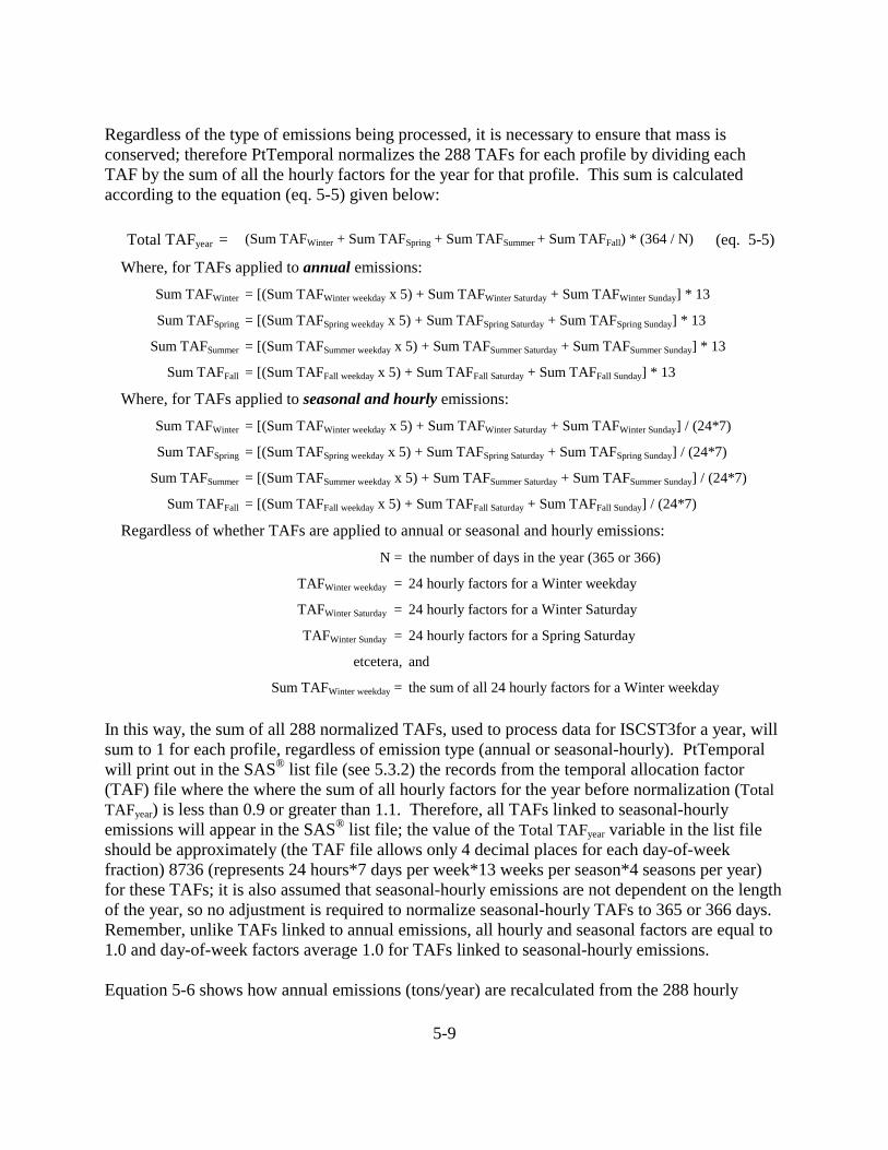
5-9
Regardless of the type of emissions being processed, it is necessary to ensure that mass is conserved; therefore PtTemporal normalizes the 288 TAFs for each profile by dividing each TAF by the sum of all the hourly factors for the year for that profile. This sum is calculated according to the equation (eq. 5-5) given below:
Total TAFyear = (Sum TAFWinter + Sum TAFSpring + Sum TAFSummer + Sum TAFFall) * (364 / N) (eq. 5-5)
Where, for TAFs applied to annual emissions: Sum TAFWinter = [(Sum TAFWinter weekday x 5) + Sum TAFWinter Saturday + Sum TAFWinter Sunday] * 13
Sum TAFSpring = [(Sum TAFSpring weekday x 5) + Sum TAFSpring Saturday + Sum TAFSpring Sunday] * 13
Sum TAFSummer = [(Sum TAFSummer weekday x 5) + Sum TAFSummer Saturday + Sum TAFSummer Sunday] * 13
Sum TAFFall = [(Sum TAFFall weekday x 5) + Sum TAFFall Saturday + Sum TAFFall Sunday] * 13
Where, for TAFs applied to seasonal and hourly emissions:
Sum TAFWinter = [(Sum TAFWinter weekday x 5) + Sum TAFWinter Saturday + Sum TAFWinter Sunday] / (24*7)
Sum TAFSpring = [(Sum TAFSpring weekday x 5) + Sum TAFSpring Saturday + Sum TAFSpring Sunday] / (24*7)
Sum TAFSummer = [(Sum TAFSummer weekday x 5) + Sum TAFSummer Saturday + Sum TAFSummer Sunday] / (24*7)
Sum TAFFall = [(Sum TAFFall weekday x 5) + Sum TAFFall Saturday + Sum TAFFall Sunday] / (24*7)
Regardless of whether TAFs are applied to annual or seasonal and hourly emissions:
N = the number of days in the year (365 or 366)
TAFWinter weekday = 24 hourly factors for a Winter weekday
TAFWinter Saturday = 24 hourly factors for a Winter Saturday
TAFWinter Sunday = 24 hourly factors for a Spring Saturday
etcetera, and
Sum TAFWinter weekday = the sum of all 24 hourly factors for a Winter weekday In this way, the sum of all 288 normalized TAFs, used to process data for ISCST3for a year, will sum to 1 for each profile, regardless of emission type (annual or seasonal-hourly). PtTemporal will print out in the SAS® list file (see 5.3.2) the records from the temporal allocation factor (TAF) file where the where the sum of all hourly factors for the year before normalization (Total TAFyear) is less than 0.9 or greater than 1.1. Therefore, all TAFs linked to seasonal-hourly emissions will appear in the SAS® list file; the value of the Total TAFyear variable in the list file should be approximately (the TAF file allows only 4 decimal places for each day-of-week fraction) 8736 (represents 24 hours*7 days per week*13 weeks per season*4 seasons per year) for these TAFs; it is also assumed that seasonal-hourly emissions are not dependent on the length of the year, so no adjustment is required to normalize seasonal-hourly TAFs to 365 or 366 days. Remember, unlike TAFs linked to annual emissions, all hourly and seasonal factors are equal to 1.0 and day-of-week factors average 1.0 for TAFs linked to seasonal-hourly emissions. Equation 5-6 shows how annual emissions (tons/year) are recalculated from the 288 hourly

5-10
emission rates (tons/hour). Note that emission totals for each season depend on exactly how many weeks are in each season.
EannC = (Winter + Spring + Summer + Autumn) (eq. 5-6)
where:
Winter = ((WinterWeekdays x 5) + WinterSaturdays + WinterSundays) x (# / 7)
Spring = ((SpringWeekdays x 5) + SpringSaturdays + SpringSundays) x (92 / 7)
Summer = ((SummerWeekdays x 5) + SummerSaturdays + SummerSundays) x (92 / 7)
Autumn = ((AutumnWeekdays x 5) + AutumnSaturdays + AutumnSundays) x (91 / 7)
# = 91 in leap years and 90 in non-leap years
WinterWeekdays = E1 + E2 + … + E24
WinterSaturdays = E97 + E98 + … + E120
WinterSundays = E193 + E194 + … + E216 5.2 How do I run PtTemporal? 5.2.1 Prepare your point source inventory for input into PtTemporal With the exception of a link-based inventory containing seasonal-hourly emissions for ISCST3 (which is discussed below), the point source inventory you use for input into PtTemporal must be the output of PtModelProc, if you intend to create ASPEN input files or the SO section of the ISCST3 run stream. If you don’t intend to create ASPEN or ISCST3 specific output by running PtFinal_ASPEN or PtFinal_ISCST3, respectively, you could use the output from PtDataProc as the input into PtTemporal. The inventory produced by either PtDataProc or PtModelProc will meet all requirements. When processing data for ASPEN, the inventory produced by PtModelProc will contain at least the variables listed in Table 5-1. It may contain additional variables such as the diagnostic flag variables (LFLAG, FIPFLAG, etc.) created by PtDataProc depending on the options you chose for the windowing function in PtDataProc (see Section 3.1.3). When processing data for ISCST3, this inventory will contain the variables listed in Table 5-2 with some exceptions. Only if you have included ISCST3 area and/or volume sources will the inventory contain the release parameter variables required for these sources (see Section 3.2.1 for a description of these source types). The inventory may contain additional variables such as the diagnostic flag variables LLPROB or FIPFLAG created by PtDataProc depending on the options you chose for the windowing function and the contents of the VARLIST ancillary file used in PtDataProc.

5-11
When processing data for ISCST3, you may have a seasonal-hourly emissions inventory consisting of onroad mobile links or grid cells; both are ISCST3 area sources with coordinates and emission arrays. These emission arrays are created using MOBILE6.2 with link-based VMT to produce (by multiplying the emission factors by VMT) a seasonal-hourly emissions inventory. In this case, PtTemporal will be the first EMS-HAP program you execute, and you are required to provide data that satisfies both Tables 5-2 and 5-3. For seasonal-hourly emissions, the EMIS variable is used strictly for quality assurance to ensure that day-of-week temporal allocations conserve emission totals. PtDataProc and PtModelProc do not support the operations needed to generate a seasonal-hourly link based inventory (e.g., running MOBILE6.2 and properly formatting the links or grid cells as ISCST3 area sources) and therefore do not need to be run. For those variables that are not associated with seasonal-hourly emissions (e.g., BLDH, BLDW, STACKHT), you must still create them (their values will be missing). You should assign the variable SRC_TYPE as “onroad”; and, the UTMX and UTMY coordinates should represent the southwest corner of each link (or grid cell) for seasonal-hourly link-based emissions. Otherwise, the UTMX and UTMY coordinates represent the center of the source. Also, recall (see Figure 2-5 in Section 2.2.3) the relationship of the orientation angle to the x (AXLEN) and y (AYLEN) dimensions of your link-based (ISC area) source. Finally, it is important that the aspect ratio of your ISCST3 source not exceed 100:1 (e.g., if axlen=25 meters, aylen must be between 0.25 and 2500 meters). Use trigonometric relationships to obtain the UTMX and UTMY coordinates if you are provided a link-based inventory containing a pair of nodes and a road width, or, if you need to split a road segment into 2 or more pieces to satisfy the 100:1 aspect ratio. Link-based emissions are modeled as ISCST3 area sources; therefore ISCTYPE should be assigned as “iscarea”. The value of the variable EMRELPTY is irrelevant for ISCST3 area sources. As is the case with all sources in the point source inventory, the value you assign to the EMRELPID and SITE_ID variables for link-based sources must be unique. The EMIS variable is used only for quality assurance for link-based processing. The variables SAROAD and NTI_HAP should be assigned to link-based emissions; you can use any of the available HAP tables (Appendix A) to obtain SAROAD and NTI_HAP codes. The SAROADDC and REACT variables are not required for ISCST3 processing; therefore, these variables do not need to be created for link-based emissions. However, all stack parameters should be initialized as missing for link-based emissions. Concatenating the point source inventory (PtModelProc output) with link-based emissions, prior to PtFinal_ISCST3 (Chapter 8), facilitates simpler construction of the SO pathway section of the ISCST3 run stream file. If you do not do this, you will need to add ISCST3 include file statements and additional source grouping definitions to the SO pathway section created from your first run of PtFinal_ISCST3.

5-12
Table 5-1. Variables in the PtTemporal Input Point Source Inventory SAS® File when Processing Data for ASPEN
Variables used by PtTemporal are in bold; other variables listed are used by previously run or subsequent point source processing programs.
Variable Name Data Description (Required units or values are in parentheses)
Type*
BLDH building height (meters) (5 for horizontal stacks, 0 for all other stacks); assigned in PtModelProc (see Section 4.1.4)
N
BLDW building width (meters) (5 for horizontal stacks, 0 for all other stacks); assigned in PtModelProc (see Section 4.1.4)
N
CNTL_EFF baseline control efficiency, expressed as a percentage N
EMIS pollutant emissions value (tons/year) N
EMRELPID code identifying a unique emission point within a site A50
EMRELPTY physical configuration code of release point (01=fugitive; 02=vertical stack; 03=horizontal stack, 04=goose neck, 05=vertical with rain cap, 06=downward-facing vent, 99=missing, AP=allocated to point during COPAX –e.g., aircraft)
A4
FIPS 5-digit FIPS code (state and county combined) A5
IBLDG building code (1 for horizontal stacks, 0 for all other stacks) assigned in PtModelProc (see Section 4.1.4)
A1
IVENT vent type (0 for stacked sources, 1 for non-stacked sources) assigned in PtModelProc (see Section 4.1.4)
A1
LAT latitude (decimal degrees) N
LON longitude (negative decimal degrees for Western Hemisphere) N
MACT MACT code A7
NTI_HAP code identifying HAP on the Clean Air Act HAP list; assigned in PtModelProc (see Section 4.1.1)
A3
REACT pollutant reactivity/particulate size class (1-9); assigned in PtModelProc (see Section 4.1.1)
N
SAROAD unique pollutant-group code; assigned in PtModelProc (see Section 4.1.1 or 4.1.2) A10
SAROADDC descriptive name for the SAROAD; assigned in PtModelProc (see Section 4.1.1) A50
SCC EPA source category code identifying the process A10
SIC Standard Industrial Classification (SIC) code for the site A4
SITE_ID code identifying a unique site A25

Table 5-1. Variables in the PtTemporal Input Point Source Inventory SAS® File when Processing Data for ASPEN (continued)
5-13
Variable Name Data Description (Required units or values are in parentheses)
Type*
SRC_TYPE description of the emission source at the site (assigned in COPAX as ‘nonroad’ for allocated nonroad or combined onroad and nonroad mobile county-level emissions; ‘area’ for allocated non-point county-level emissions). If you choose to define source groups by this variable as explained in 8.1.1, or run PtGrowCntl (Chapter 6) then it must have the value of ‘major’ or ‘area’ for non-allocated emissions. Must have the value of ‘onroad’ for onroad segment emissions (see Section 5.2.1).
A15
STACKDIA diameter of stack (meters) N
STACKHT height of stack (meters) N
STACKVEL velocity of exhaust gas stream (meters per second) N
STKTEMP temperature of exhaust gas stream (Kelvin) N
UFLAG urban/rural dispersion flag (1 for urban, 2 for rural); assigned in PtModelProc (see Section 4.1.2)
N
* Ax = character string of length x, N = numeric

5-14
Table 5-2. Variables in the PtTemporal Input Point Source Inventory SAS® File when Processing Data for ISCST3
Variables used by PtTemporal are in bold; other variables listed are used by previously run or subsequent point source processing programs.
Variable Name Data Description (Required units or values are in parentheses)
Type*
AANGLEc orientation angle of rectangle for ISCST3 area source (degrees from North) N
AINPLUMc initial vertical dimension of ISCST3 area source plume (meters) N
ARELHGTa release height of ISCST3 area source (meters) N
AXLENa length of X side of ISCST3 area source (meters) N
AYLENc length of Y side of ISCST3 area source (meters) N
BLDH building height (meters); missing values defaulted in PtModelProc (see Section 4.1.3) or pre-processing program for season-hourly emissions
N
BLDW building width (meters); missing values defaulted in PtModelProc (see Section 4.1.3) or pre-processing program for season-hourly emissions
N
CNTL_EFF baseline control efficiency, expressed as a percentage N
EMIS pollutant emissions value (tons/year) N
EMRELPID code identifying a unique emission point within a site A50
EMRELPTY (01=fugitive; 02=vertical stack; 03=horizontal stack, 04=goose neck, 05=vertical with rain cap, 06=downward-facing vent, 99=missing, AP=allocated to point during COPAX –e.g., aircraft)
A4
FIPS 5-digit FIPS code (state and county combined) A5
ISCTYPEa,b ISCST3 source type (iscarea or iscvolume) A9
MACT MACT code A7
NTI_HAP code identifying HAP on the Clean Air Act HAP list; assigned in PtModelProc (see Section 4.1.1) except for link-based emissions
A3
REACT pollutant reactivity/particulate size class (1-9); assigned in PtModelProc (see Section 4.1.1) except for link-based emissions
N
SAROAD unique pollutant-group code; assigned in PtModelProc (see Section 4.1.1) except for link-based emissions
A10
SAROADDC descriptive name for the SAROAD; assigned in PtModelProc (see Section 4.1.1) except for link-based emissions
A50
SCC EPA source category code identifying the process A10
SIC Standard Industrial Classification (SIC) code for the site A4
SIGMAXb initial lateral dimension of volume source (meters) N
SIGMAZb initial vertical dimension of volume source (meters) N
SITE_ID code identifying a unique site A25

Table 5-2. Variables in the PtTemporal Input Point Source Inventory SAS® File when Processing Data for ISCST3 (continued)
5-15
Variable Name Data Description (Required units or values are in parentheses)
Type*
SRC_TYPE description of the emission source at the site (i.e., ‘nonroad’ for allocated nonroad or combined onroad and nonroad mobile county-level emissions; ‘area’ for allocated non-point county-level emissions). If you choose to define source groups by this variable as explained in 8.1.1, or run PtGrowCntl (Chapter 6) then it must have the value of ‘major’ or ‘area’ for non-allocated emissions. Assign as ‘onroad’ for link-based MOBILE6.2 emissions.
A15
STACKDIA diameter of stack (meters) N
STACKHT height of stack (meters) N
STACKVEL velocity of exhaust gas stream (meters per second) N
STKTEMP temperature of exhaust gas stream (Kelvin) N
UTMX UTM easting (meters) of southwest corner of source for link-based emissions, and of center of source for all other emissions
N
UTMY UTM northing (meters) of southwest corner of source for link-based emissions, and of center of source for all other emissions
N
VOLHGTb release height above ground for volume source (meters) N
* Ax = character string of length x, N = numeric a variables required for processing ISCST3 area sources b variables required for processing ISCST3 volume sources c additional variables only included when information is available Table 5-3. Additional Required Variables in the PtTemporal Input Point Source
Inventory SAS® File when Processing Seasonal-Hourly Data for ISCST3
Variable Name
Data Description (Required units or values are in parentheses)
Type*
WINTER1,…WINTER24
array of 24 hourly winter emissions (tons/hour); with the first representing 12 midnight to 1am. for example, winter14 represents hourly winter emissions for 2pm local time
N
SPRING1,… SPRING24
array of 24 hourly spring emissions (tons/hour) N
SUMMER1,…SUMMER24
array of 24 hourly summer emissions (tons/hour) N
AUTUMN1,…AUTUMN24
array of 24 hourly autumn emissions (tons/hour) N
N = numeric; Winter includes December, January, February; Spring includes March, April, May; Summer includes June July, August; Fall includes September, October, November 5.2.2 Determine whether you need to modify the ancillary input files for PtTemporal An ancillary file is any data file you input to the program other than your emission inventory. Table 5-4 lists the ancillary input files required for PtTemporal and when you may need to modify the files these keywords represent. Appendix A contains ancillary file formats, and Appendix C

5-16
discusses the development of ancillary files supplied with EMS-HAP.
Table 5-4. Ancillary Input File Keywords for PtTemporal
File Keyword
Purpose Need to Modify Files Supplied with EMS-HAP?
TAF ASPEN file: Provides temporal profiles containing 24 hourly temporal allocation factors (TAFs) for an average day by SCC and/or AMS codes
ISCST3 file: Provides temporal profiles containing seasonal allocation factors, day-type allocation factors, and hourly allocation factors by SCC and/or AMS codes
When additional source specific temporal factors become available
SCCLINK Provides cross reference between SCC on inventory to SCC and/or AMS on TAF file in order to assign temporal profile
When inventory contains records with partial SCC codes, or SCC codes that are not in the cross-reference file or TAF file
SICLINK Provides cross reference between SIC on inventory to SCC and/or AMS on TAF file in order to assign temporal profile
When inventory contains records with the source category identified by SIC codes that may be useful for matching in cases where the SCC doesn’t match
MACTLINK Provides cross reference between MACT code on inventory to SCC and/or AMS on TAF file in order to assign temporal profile
When inventory contains records with the source category identified by the MACT category codes that may be useful for matching in cases where the SCC doesn’t match
5.2.3 Modify the temporal allocation factor file (keyword TAF) The temporal allocation factor (TAF) file is common to point, non-point and mobile source emission processing within EMS-HAP. Two TAF files are supplied with EMS-HAP: one is for use with ASPEN, and contains hourly factors only, and the other is for use with ISCST3, which contains seasonal, day type, and hourly factors. In both ASPEN and ISCST3 TAF files, local time zones are used. 8-digit SCC or 10-digit AMS codes index the temporal profiles. The profiles in the ISCST3 TAF file must have unique codes for those profiles used to process the seasonal-hourly (link-based or grid cell) emissions for ISCST3. For example, you could assign an “SCC” of “ONRD_TAF1” for a particular set of records in the input inventory with the same day-of-week temporal characteristics such as total light duty gasoline vehicles (SCC=2201001000) and then use that code to the ISCST3 TAF file. Note that in the link-based emission file you are inputting to PtTemporal, the SCC should be defined differently than they way you define it for the non-link-based emissions. Also, remember that hourly and seasonal temporal factors must equal 1.0 (see Section 5.1.3) for all seasonal-hourly input emissions. Whether to modify or add to the temporal profiles contained within the TAF files supplied with

5-17
EMS-HAP depends on the information you have on the temporal characteristics of specific source categories and how well the source category information included in your emission inventory matches to the existing profiles. For example, you might consider modifying the TAF file if you find, that after executing PtTemporal, a large number of records with some form of source category information cannot be matched to a temporal profile and, therefore, are being assigned a uniform profile. You can determine which records are being assigned a uniform profile by looking at the log and list files and a special SAS® file named “notaf” created when you run PtTemporal (see Section 5.3.3 for more details).
5.2.4 Modify the cross-reference files used to link inventory records to the temporal allocation factor file (ancillary file keywords SCCLINK, SICLINK, and MACTLINK)
PtTemporal uses three cross-reference files for cases where the SCC is missing or the value contained on the emission inventory record can’t be linked directly to the SCC and/or AMS on the TAF file. These cross-reference files provided with EMS-HAP were developed to accommodate the types of source category information included in the July 2001 version of the 1996 NTI. For instance, this inventory does not include a value for the SCC for every emission record or sometimes uses a shortened 1-digit, 3-digit or 6-digit SCC. Therefore, one cross-reference file (keyword SCCLINK) links generic 1-digit, 3-digit, and 6-digit SCCs to the 8-digit SCC and 10-digit AMS codes used in the temporal profile file. Another file (keyword SICLINK) links SIC codes to SCC and AMS codes, and is used in cases where no SCC is included on the emission record, but an SIC is included. A third file (keyword MACTLINK) links MACT codes to SCC and AMS codes and is used for cases where no SCC code is present on the emission record, but a MACT code is available. The same files can be used when processing data for ASPEN and for ISCST3. You would expect to modify any of these files depending on the source category information included in your emission inventory. You might consider modifying these files after executing PtTemporal if you find that a large number of records with some form of source category information cannot be matched to a temporal profile and, therefore, are being assigned a uniform profile. You can determine which records are being assigned a uniform profile by looking at the log and list files and a special SAS® file named “notaf” created when you run PtTemporal (see Section 5.3.3 for more details).
5.2.5 Prepare your batch file The batch file serves two purposes: (1) allows you to pass “keywords” such as file names and locations, program options, and run identifiers to the program, and (2) sets up the execute statement for the program. Sample batch files for PtTemporal for ASPEN and ISCST3 emissions processing are shown in Figures B-8 and B-9, respectively, of Appendix B. The best way to prepare your batch file is to copy one of the samples we provide and modify it to fit your needs. Specify your keywords Table 5-5 describes the keywords required in the batch file. Use keywords to locate and name all

5-18
input and output files. The same batch file can be used for running PtTemporal for ASPEN or ISCST3. The only differences are in the assignment of the keywords MODEL (either ‘ASPEN’ or ‘ISC’), the presence of the LEAPYEAR keyword for ISCST3 processing only, and TAF (different TAF files are used for ASPEN and ISCST3, see Section 5.2.3).
Table 5-5. Keywords in the PtTemporal Batch File when Processing Data for Either ASPEN or ISCST3
Keyword Description of Value Input Inventory Files IN_DATA Name of directory containing the input inventory SAS® file INSAS Input inventory SAS® file name, prefix of file name only Ancillary Files REFFILE Name of directory containing the ancillary files TAF Temporal profile text file, prefix only (note that different files are used for ASPEN data
processing and ISCST3 data processing) SCCLINK SCC to SCC or AMS cross-reference text file, prefix only SICLINK SIC to SCC or AMS code cross-reference text file, prefix only MACTLINK MACT category code to SCC or AMS cross-reference text file, prefix only Program Options MODEL ASPEN=process data for ASPEN model; ISC=process data for ISCST3 model LEAPYEAR* 1 = yes, model year is leap year (366 days; i.e., 1996), 0 = non-leap year (365 days) Output files OUTDATA Name of directory containing the output inventory SAS® file OUTSAS Output inventory SAS® file name, prefix only
* ISCST3 processing only Prepare the execute statement The last line in the batch file runs the PtTemporal program. In the sample batch files provided in Figures B-8 and B-9 of Appendix B, you will see a line preceding the run line that creates a copy of the PtTemporal code having a unique name. It is this version of the program that is then executed in the last line. If you do this, the log and list files created by this run can be identified by this unique name. If you don’t do this and run the program under a general name, every run of PtTemporal will create a log and list file that will replace any existing files of the same name. You may find that you need to assign a special area on your hard disk to use as workspace when running PtTemporal. In the sample batch file, a work directory is defined on the last line following the execution of PtTemporal. For example, the command ‘sas PtTemporal_062000.sas -work /data/work15/dyl/’ assigns a SAS® work directory in the “/data/work1/dyl” directory. The directory you reference must be created prior to running the program.

5-19
5.2.6 Execute PtTemporal There are two ways to execute the batch file. One way is to type ‘source’ and then the batch file name. Alternatively, first set the permission on the file to ‘execute.’ You do this by using the UNIX chmod command and adding the execute permission to yourself, as the owner of the file, to anyone in your user group, and/or to anyone on the system. For example, ‘chmod u+x PtTemporal.bat’ gives you permission to execute the batch file. Refer to your UNIX manual for setting other permissions. After you have set the file permission, you can execute the batch file by typing the file name on the command line, for example, ‘PtTemporal.bat’. 5.3 How Do I Know My Run of PtTemporal Was Successful? 5.3.1 Check your SAS® log file You need to review the output log file to check for errors or other flags indicating incorrect processing. This review should include searching the log files for occurrences of the strings “ERROR”, “WARNING”, “not found”, and “uninitialized”. These can indicate problems with input files or other errors. You can look at the number of records in the input inventory file and compare it to the number of records in the output inventory file. The number of records should be the same in these two files. 5.3.2 Check your SAS® list file The list file created when PtTemporal is executed contains information to assist in quality assurance. The information is this file is listed below. $ When processing data for ASPEN, a list of records from the temporal allocation factor (TAF)
file where the average of the 3-hour factors before normalization is less than 0.9 or greater than 1.1
$ When processing data for ISCST3, a list of records from the temporal allocation factor (TAF) file where the sum of all hourly factors for the year before normalization is less than 0.9 or greater than 1.1. Note, all TAFs linked to seasonal-hourly emissions should appear in the SAS® list file; the value of the Total TAFyear variable in the list file should be approximately 8736 (represents 24 hours*7 days per week*13 weeks per season*4 seasons per year) for these TAFs.
C Annual emission totals of the temporally allocated emissions and the unmatched (uniformly allocated by default) emissions by SAROAD code
5.3.3 Check other output files from PtTemporal You should check for the existence of the output inventory file named by keyword OUTSAS. This file will serve as the input to the next point source processing program you choose to run. PtTemporal also creates a SAS® output file named “notaf” if emission records are not assigned a specific temporal profile. For these records, emissions were uniformly allocated to each of the

5-20
time periods. You can reduce the number of records appearing in this file by the following: 1) modify the TAF ancillary file we supplied by adding SCC codes and corresponding temporal allocation factors; 2) modify one of the ancillary cross-reference files (keywords SCCLINK, SICLINK, MACTLINK) in order to link an AMS or SCC code in the TAF file with the source or process information contained on the emission records (i.e., SCC, SIC, or MACT).

6-1
CHAPTER 6
Point Source Processing The Growth and Control Program (PtGrowCntl)
The flowcharts below (Figure 6-1) show how PtGrowCntl fits into EMS-HAP’s point source processing for the ASPEN and ISCST3 models. The point source inventory you input to PtGrowCntl is the output from PtTemporal (Chapter 5). You use the output inventory from PtGrowCntl as the input to PtFinal_ASPEN (Chapter 7) when processing data for ASPEN and PtFinal_ISCST3 (Chapter 8) when processing data for ISCST3.
PtDataProc
PtModelProc
PtTemporal
PtGrowCntl
PtFinal_ASPEN
OR
Point source emissions
ASPEN point source emission files
PtFinal_ISCST3
ISCST3 SO pathway of run stream section for ISCST3 point, volume, and area sources
Flowchart for ASPEN Processing Flowchart for ISCST3 Processing
Point source emissions
PtDataProc
PtModelProc
PtTemporal
PtGrowCntlOR
Figure 6-1. Overview of PtGrowCntl within EMS-HAP Point Source Processing

6-2
6.1 What is the function of PtGrowCntl? The Growth and Control Program (PtGrowCntl) computes future year (or projected) emissions as a result of projected economic growth and/or emission reduction strategy scenarios. PtGrowCntl can develop multiple sets of future-year emission files in a single run through the use of a comma-delimited ancillary file (keyword PROJECT), which allows you to specify multiple projection scenarios. Each record in the PROJECT file contains all growth and/or emission reduction strategy scenario information for a particular projection scenario. For each projection scenario in the PROJECT file, you can apply growth factors by site (SITE_ID variable), Maximum Achievable Control Technology (MACT), SIC, and/or SCC codes, and you can apply reduction percentages based on the MACT standards and/or based on your own control strategy. You control the growth and control functions listed below in any given execution of PtGrowCntl through the ancillary files and parameters you supply in the batch file (see Tables 6-12 and 6-13 in Section 6.2.6 for details on how to do this). The following bullets list the functions of PtGrowCntl.
C PtGrowCntl determines a projection scenario for each record in the PROJECT ancillary file
C For each scenario, PtGrowCntl assigns and applies growth factors to project emissions
due to growth C For each scenario, PtGrowCntl assigns MACT-based emission reduction information C For each scenario, PtGrowCntl assigns user-defined emission reduction information C For each scenario, PtGrowCntl combines MACT-based and user-defined emission
reduction information and applies to grown emissions to project emissions for that scenario
Figure 6-2 shows the flowchart of PtGrowCntl when processing data for ASPEN or ISCST3. The processing steps are the same when processing data for either model, although you still need to identify the model as being either ‘ASPEN’ or ‘ISC’ through the batch file keyword MODEL (see Section 6.2.6). The following sections describe the above bullets.

6-3
Figure 6-2. PtGrowCntl Flowchart when Processing Data for ASPEN and ISCST3
Reads keywordsBatch file containing keywords relevant to all projection scenarios; e.g., input file name, directory paths, comma-delimited file (keyword PROJECT) containing information on all projection scenarios
For each record in the PROJECT file: output point source inventory file; name is keyword OUTSAS appended with
the value of PNAME parameter in PROJECT
PtGrowCntl: MACRO APPLCNTL For each record in the PROJECT file: calculates projected emissions from temporally allocated baseline emissions.
General MACT reduction control information file
(MACTGEN in PROJECT)
Specific process/pollutant MACT reduction control information file
(SPECFILE in PROJECT)
PtGrowCntl: MACRO GROW For each record in the PROJECT file: (1) reads SITE_ID, MACT, SIC, and SCC growth factor files; (2) assigns growth factors first by SITE_ID, then MACT (if necessary), then SIC (if necessary), and finally SCC code if growth factors by SITE_ID, MACT and SIC have not been applied. MACT, SIC, and SCC growth factors are applied nationally, by state FIPS, and/or by county FIPS.
Point source inventory file (keyword INSAS)
PtGrowCntl: MACRO MACTCNTL For each record in the PROJECT file: (1) reads general MACT reduction control information file and assigns control information to emission records by MACT category; (2) reads specific process/pollutant MACT reduction control information file and assigns control information to emission records by MACT category and pollutant and/or process codes.
PtGrowCntl: MACRO USERCNTL For each record in the PROJECT file: reads user-defined reduction control information file and assigns control information to emission records by county, MACT code, SCC code, SIC code, pollutant and/or process codes.
SIC growth factor file (GFSIC in PROJECT)
SCC growth factor file (GFSCC in PROJECT)
MACT category growth factor file (GFMACT in PROJECT)
SITE ID growth factor file (GFSITE in PROJECT)
User-defined reduction control information file
(USERFILE in PROJECT)
FIPS to county control code cross-reference file
(CNTYUR in PROJECT)
PtGrowCntl: MACRO GETINFO Reads point source inventory file and comma-delimited ancillary file (keyword PROJECT) containing projection scenarios in each record. Fields in PROJECT contain all ancillary and output file names and projection scenario options.
For each record in the PROJECT file
For
eac
h re
cord
in th
e PR
OJE
CT fi
le

6-4
6.1.1 PtGrowCntl determines a projection scenario for each record in the PROJECT ancillary file
PtGrowCntl uses a comma-delimited ancillary file (keyword PROJECT) to determine the projection scenarios for which to compute future year emissions. Each record in the PROJECT file contains all growth and/or emission reduction strategy scenario information, consisting of ancillary file names and parameters, which define a particular projection scenario. PtGrowCntl will output a separate projected inventory file for each projection scenario in PROJECT. This allows you to project to several different future years in a single run. For each projection scenario in the PROJECT file, you can apply growth factors by facility (SITE_ID variable), MACT, SIC, and/or SCC codes; and, you can apply reduction percentages based on MACT standards and/or based on your own control strategy. Each record in the PROJECT file includes the appropriate file names and parameters PtGrowCntl will use for computing the particular scenario. Table 6-1 describes these files and parameters (in the necessary order for the comma delimited PROJECT file) and shows sample values for sample scenarios. The header row displays the logical names used for these files and parameters in the PtGrowCntl code; we refer to these projection scenario variables by these names throughout this chapter. The first four fields in Table 6-1, GFSITE, GFMACT, GFSIC, and GFSCC represent file names containing growth factor information by SITE_ID, MACT, SIC, and/or SCC code variables, respectively. Section 6.1.2 discusses how PtGrowCntl uses this information to grow your inventory. In the second projection scenario in Table 6-1, the value for GFSITE is missing. This means the user did not supply a file containing site-specific growth factors, so no sources will be grown with site-specific information. In the actual PROJECT file, you can enter the word “NONE” or put nothing between the commas to indicate that a particular file is not used. The next six fields in Table 6-1, MACTGEN, SPECFILE, USERFILE, CNTYUR, GROWYEAR, and YEARTYPE, provide MACT-based and user-defined emission reduction information; these are discussed in Sections 6.1.3 and 6.1.4. The output filename for each projection scenario is the value of the batch file keyword OUTSAS appended with the value for PNAME. For example, if OUTSAS is “proj_pt_”, then for the third projection scenario in Table 6-1 (last row of table), PtGrowCntl will produce a SAS® output base filename of “proj_pt_gc03fm2”. Finally, the COMMENTS field in Table 6-1 provides the first line title for each output in the SAS® list file pertaining to the projection scenario being executed. From this point forward, all projection scenario variables referenced in the PROJECT file will be referred to as their field names (header row) in Table 6-1. For example, the term “GFMACT” will refer to the MACT-based growth factor file discussed in the following section.

6-5
Table 6-1. Information in the PROJECT File and Sample Values
Projection Scenario Variables GFSITE GFMACT GFSIC GFSCC MACTGEN SPECFILE USERFILE CNTYUR GROWYEAR YEARTYPE PNAME COMMENTS file: site-level growth factors
file: FIPS/ MACT level growth factors
file: FIPS/ SIC level growth factors
file: FIPS/ SCC level growth factors
file: MACT generalcontrols
file: MACT specific controls (SCC and/or HAP)
file: User-defined controls
file: county-code assignments associated with any county-related user-defined controls in USERFILE; ignored if USERFILE is ‘NONE’ or left blank
Parameter: Year you want to project to
Parameter: "CALENDAR" or "FISCAL" The FISCAL year is from Oct. 1 to Sept. 30.
parameter: suffix of the output file name for output inventory containing Base/Projected emissions
parameter string of words: comment is used for titles in the list file output
Sample Projection Scenarios
gf99site_07 gf99mact_07 gf99sic_07 gf99scc_07
MACT_gen_base99_c2007
MACT_spec_base99_c2007 popflg99 2007 CALENDAR gc07fm2
2007 – CALENDAR. Growth: SITE_ID, MACT, SIC + SCC. Control: MACT gen + spec
gf99mact_02 gf99sic_02 gf99scc_02MACT_gen_base99_c2002
MACT_spec_base99_c2002 2002 CALENDAR gc02fm2
2002 – CALENDAR. Growth: MACT,SIC + SCC. Control: MACT gen + spec
gf99mact_03 gf99sic_03 gf99scc_03MACT_gen_base99_c2003
MACT_spec_base99_c2003 2003 CALENDAR gc03fm2
2003 – CALENDAR. Growth: MACT,SIC + SCC. Control: MACT gen + spec

6-6
6.1.2 For each scenario, PtGrowCntl assigns and applies growth factors to project emissions due to growth
PtGrowCntl assigns growth factors to the emission records based on the site ID (inventory SITE_ID variable), MACT category, the SIC code, and/or the SCC. MACT, SIC, and SCC-based growth factors allow for geographic resolution at the national, state or county level. You control how PtGrowCntl assigns growth factors for each projection scenario in the PROJECT file by supplying the appropriate growth factor files, and including the names of these files in the PROJECT file. The first four comma-delimited entries in each row of the PROJECT file, GFSITE, GFMACT, GFSIC, and GFSCC, provide the text ancillary growth factor files by SITE_ID, MACT, SIC, and SCC, respectively, that are used for each particular projection scenario. A growth factor file is not applied if the value for one of these fields is blank or set to “NONE”. In addition, the hierarchy of growth factors, provided in Table 6-2, is such that lower order growth factors do not replace higher order growth factors; for instance, MACT-based growth factors never replace site-level (SITE_ID) growth factors, and SIC growth factors never replace MACT-based growth factors.
Table 6-2. Growth Factor Application Information and Order of Precedence
Order of Precedence
Site ID
MACT: county-
level
MACT: state-level
MACT: US-level
SIC: county-
level
SIC: state-level
SIC: US-level
SCC: county-
level
SCC: state-level
SCC: US-level
1 (most specific, supercedes all others) X 2 X 3 X 4 X 5 X 6 X 7 X 8 X 9 X
10 (least specific information) X MACT-based, SIC-based, and SCC-based growth factors can be applied to specific geographic regions: nationally, by state, or by county (see Section 6.2.3 for more details). As seen in Table 6-2, in each case, the more detailed growth factor (e.g., county) will replace the less detailed one (e.g., state). The SITE_ID, MACT, SIC, and SCC-based growth factor files are specific to both the base year and future year. Thus, the growth factor files you supply for a particular scenario must contain growth factors specific to both the particular base year and to the particular future year for the scenario for which you use them. You can grow to different years within a single run of PtGrowCntl by supplying separate sets of SITE_ID, MACT, SIC, and SCC-based growth factor

6-7
files and using these for separate projection scenarios in the PROJECT file. PtGrowCntl computes grown, temporally allocated emission rates (eight 3-hour average emission rates when processing data for ASPEN, and 288 hourly specific emission rates when processing data for ISCST3) for each record by multiplying the base year temporally allocated emission rates by the assigned growth factor, as follows: Grown emissions = (Base year emissions) x (Growth factor) The same growth factor is applied to all temporally allocated emission rates comprising a specific inventory record. Note that any record not assigned a growth factor based either on the SITE_ID, MACT, SIC, or SCC variables will be assigned the default growth factor of one. In these cases, the grown emissions will be unchanged from the base year emissions. In addition, for any scenarios in which you do not supply any growth factor files, grown emissions will be unchanged from the base year emissions.
6.1.3 For each scenario, PtGrowCntl assigns MACT-based emission reduction information
For each scenario in the PROJECT file, PtGrowCntl can assign MACT-based emission reduction information to the point source inventory alone or along with the assignment of your own control strategy (user-defined emission reduction information). You choose the method through the MACTGEN, SPECFILE and USERFILE fields in the PROJECT file (see Tables 6-1 and 6-13). This section describes the assignment of MACT reduction information through the MACTGEN and SPECFILE files. MACTGEN represents the file containing general MACT information and SPECFILE represents the file containing specific (i.e., specific to different pollutants and processes within a MACT category) information. We first describe the general MACT information. PtGrowCntl will apply MACT reduction information for a particular scenario from the MACTGEN file you supply for that scenario. This information will not be applied if the MACTGEN field is equal to ‘NONE’ or is left blank. The general emission reduction information you supply for each MACT category in the MACTGEN ancillary file consists of:
$ Two control efficiencies for the reduction strategy. One efficiency represents the emission reduction to be applied to existing sources; the other represents the emission reduction to be applied to new sources. PtGrowCntl gives you the flexibility to apply different efficiencies for new versus existing facilities because air pollution regulations often require higher emission control efficiencies for new facilities than for existing facilities. PtGrowCntl assumes that all new point sources are located at existing point sources. This would occur, for example, if an existing source rebuilt or constructed an additional operation to the extent that it (or part of it) would be considered a new source.
$ Percentage of emissions at existing sources that will come from new sources.

6-8
PtGrowCntl uses this information to apportion the emissions into new source versus existing source emissions for each inventory record. A value of 100% would mean that in the future year, the entire MACT category rebuilt to the extent that the efficiency for new sources would apply. A value of 50% would signify that half of the emissions were due to new sources at the existing facilities and the other half were from the existing part.
$ Application control flag. PtGrowCntl uses this flag to determine whether or not to apply
the control efficiencies. This enables you to keep a particular emission reduction record that you’ve put in an ancillary file, but not use it for a particular projection scenario. An example of this would be if you want to keep in your MACTGEN file, MACT-based information for a category for which the compliance date is prior to the base year, but you don’t want to apply the information since the base-year should already account for it and no future reductions for that category would be expected.
$ Source control flag. This flag determines to which source type (majora versus both areab
and major) the MACT control efficiencies apply. For example, if a particular MACT standard affects only major sources, then you’d set the source control flag to “M” in the MACTGEN file and the efficiencies would only be applied to inventory records with a source type of “major”. If a particular MACT standard affects both major and area sources, then you would set the source control flag to “B” in the MACTGEN file and the efficiencies would be applied to both source types.
$ Compliance date for the standard. PtGrowCntl uses this information along with the
projection year to determine whether or not the standard will affect the projected emissions. EMS-HAP gives you the option of projecting based on a fiscal year or a calendar year (see Table 6-13 in Section 6.2.6). If the compliance date is within the projection year, then PtGrowCntl assigns a prorated reduction based on the portion (based on the fraction of days) of either the fiscal or calendar year (based on your choice of the YEAR type parameter in the PROJECT file) that occurred prior to the compliance date. Note that the prorated reduction is applied uniformly to the temporally allocated emissions throughout the year. Thus, although this approach approximates a correct annual emissions value, it underestimates the emission rates prior to the compliance date and overestimates them after the compliance date; this is only an issue for subannual emissions used with ISCST3, since ASPEN emissions are for an annually averaged day, rather than specific hours of a specific year. If there is no compliance date in the MACTGEN ancillary file, then PtGrowCntl does not apply any reductions.
Based on the information in the MACTGEN file, the general MACT reductions (or a pro-ration a “…any stationary source or group of stationary sources located within a contiguous area and under common control that emits or has the potential to emit considering controls, in the aggregate, 10 tons per year or more of any hazardous air pollutant or 25 tons per year or more of any combination of hazardous air pollutants…” b “…any stationary source of hazardous air pollutants that is not a major source… shall not include motor vehicles or nonroad vehicles subject to regulation under title II…”

6-9
of them, as described in the last bullet above) can only be assigned to the emission inventory for a particular scenario when the following criteria are met:
$ The application control flag is equal to 1. $ The MACT compliance date occurs within or before the projection (calendar or fiscal)
year. $ The source control flag is applicable to the inventory source type. For example, if the
source control flag for a particular MACT code is “M” then the reduction will only be applied to an inventory record with that MACT code where the source type variable is ‘major’. If the source control flag is “B” (meaning both) the reduction will be applied to both major and area sources.
PtGrowCntl can apply more specific MACT-based reduction information to the emissions that applies to specific pollutants or specific processes within a MACT category. PtGrowCntl uses information in the SPECFILE ancillary text file to do this. For each MACT code, you can specify the reduction information by various combinations of the following types of information:
$ process (6-digit SCC code or 8-digit SCC code) $ pollutant (NTI_HAP variable, assigned in PtModelProc)
If you need to apply reduction information at the site-level within a MACT category, you will need to use the user-defined emission reduction information (see Section 6.1.4). It is important to note that if you choose to apply MACT-based reduction information, PtGrowCntl will always use the MACTGEN file, but will only use the SPECFILE file if its value is not blank nor set equal to ‘NONE’ in the PROJECT file. The MACTGEN file is used to determine the reduction for any pollutant (or process) within a MACT category that is not in the SPECFILE file. In addition PtGrowCntl reads the compliance date from the MACTGEN file (it is not a field in the SPECFILE file). Thus, you must make sure that any MACT category in the SPECFILE file is also in the MACTGEN file. PtGrowCntl uses the same criteria for assigning specific MACT reduction information as it does for the general information (see the three bullets above). When both general and specific reduction information can be assigned to the same inventory record, PtGrowCntl will assign the specific MACT information from the SPECFILE ancillary file over the general information. It is also possible that more than one record in the SPECFILE file (e.g., a process-specific reduction and a HAP-specific reduction) could apply to an inventory record. In this case, the more specific information replaces the less specific information. Table 6-3 shows the order of precedence followed in PtGrowCntl.

6-10
Table 6-3. Order of Precedence for MACT-based Emission Reduction Information
Information Used to Specify Reduction Information
Order of Precedence
MACT HAP 6-digit SCC
8-digit SCC
1 (most specific information, supercedes all others)
X X X
2 X X X
3 X X
4 X X
5 X X
6 (least specific information)
X
6.1.4 For each scenario, PtGrowCntl assigns user-defined emission reduction information
PtGrowCntl can assign, for each projection scenario in the PROJECT file, your own control strategy (user-defined emission reduction information) to the point source inventory with or without the inclusion of the MACT-based emission reduction information described above. You choose the method of applying reduction information by specifying the name of the user-supplied reduction file in the PROJECT file (see USERFILE in Tables 6-1 and 6-13). For each projection scenario, PtGrowCntl uses the ancillary text file USERFILE (if it is not blank nor equal to ‘NONE’), from the PROJECT file, to assign user-defined reduction information. The emission reduction information you supply in the USERFILE ancillary file consists of:
$ Two control efficiencies for the reduction strategy. Same as in the MACT reduction information described in Section 6.1.3.
$ Percentage of emissions at existing sources that will come from new sources. Same as in
the MACT reduction information described in Section 6.1.3. $ Application control flag. Same as in the MACT reduction information described in
Section 6.1.3.
$ Replacement flag. This flag lets you decide whether to have a user-defined control efficiency replace a MACT-based control efficiency (flag value ‘R’) or be applied in addition to it (flag value ‘A’). For example, you would set this flag to ‘R’ for a strategy that contains reduction information on how a particular site’s emissions will be reduced by a particular MACT standard. This setting would allow you to use site-specific MACT reduction information in lieu of the general or pollutant, process-specific MACT reduction discussed in 6.1.3.

.
6-11
You can assign emission reduction information based on your own control strategy (user-defined information) to the point source inventory alone or in addition to the assignment of MACT-based emission reduction information. The assignment of the user-defined reduction information is made independent from the assignment of the MACT-based information. After the assignment of all emission reduction information, PtGrowCntl determines which control efficiencies are used to calculate the projected emissions for each record. The user-defined reduction information can only be assigned when the user-defined application control flag is equal to 1. Through the user-defined reduction information, you can assign emission reduction information by various combinations of the following types of information:
$ broad industry group and/or process (using the SIC, MACT code and/or SCC) $ site (using the SITE_ID variable) $ pollutant (using the NTI_HAP variable) $ specific county or county types (using the CNTYCODE variable)
The specific combinations of these variables used by PtGrowCntl to match the emission reduction information to the inventory are presented in Table 6-4. In cases where more than one record in the user-defined reduction information file can be assigned to a single emission inventory record, PtGrowCntl follows a specific order of precedence as shown in Table 6-4.

6-12
Table 6-4. User-defined Emission Reduction Information and Order of Precedence
Information Used to Specify Reduction Information Order of Precedence
Site ID MACT SIC SCC HAP County Code
1 (most specific information, supercedes all others) X X X X 2 X X X 3 X X X 4 X X 5 X X X 6 X X 7 X X 8 X 9 X X X X X
10 X X X X 11 X X X X12 X X X 13 X X X X14 X X X 15 X X X16 X X 17 X X X X18 X X X 19 X X X20 X X 21 X X X22 X X 23 X X24 X 25 X X X X26 X X X 27 X X X28 X X 29 X X X 30 X X 31 X X X 32 X X 33 X X 34 X 35 X X 36 X 37 X X
38 (least specific information) X
In order to assign reduction information to specific counties or to groups of county types, you must provide the values for the five-character county type code (CNTYCODE) in the ancillary text file CNTYUR, from the PROJECT file (see Table 6-1, column 8) for each county to which you want to apply controls. PtGrowCntl uses the CNTYUR file to assign the CNTYCODE variable to the inventory by the state and county FIPS code. CNTYCODE can identify general types of counties to which you want to assign specific reduction information, such as urban or rural counties, or it can identify an individual county. These county type codes can then be used

.
6-13
in the user-defined emission reduction information (USERFILE) file. When you provide site-level reduction information, you don’t need to use a county code, because the SITE_ID variable identifies an individual site located in a specific county. Also, if user-defined reduction information is not applied (USERFILE equals ‘NONE’ or is left blank), the entry for CNTYUR in PROJECT will be ignored.
6.1.5 For each scenario, PtGrowCntl combines MACT-based and user-defined emission reduction information and applies to grown emissions to project emissions for that scenario
After all MACT-based and user-defined reduction information has been assigned to the inventory for a given projection scenario, PtGrowCntl combines the information in order to assign the “primary” reduction variables (applied to the emissions first) and the “additional” reduction variables (applied second, and in addition to primary, if necessary). PtGrowCntl calculates projected emissions by first applying primary reduction efficiencies for existing and new sources based on the percentage of projected emissions attributed to the new sources (primary reduction variables are EXISTEFF, NEW_EFF, and NEW_RATE). Depending upon how you have chosen to combine MACT-based and user-defined control scenarios, PtGrowCntl will apply additional reduction efficiencies for existing and new sources to the initially projected emissions in a similar manner (additional reduction variables are ADDXEFF, ADDNEFF, and ADDRATE). Thus, additional reductions are applied on top of the primary reductions. Assignment of Primary Reduction Efficiencies and Additional Reduction Efficiencies For each projection scenario, there are three possible ways to assign the primary and additional reduction variables depending on the contents of the files you provide to PtGrowCntl through the PROJECT file. These are described below. $ Using only MACT-based reduction information: the MACT-based reduction efficiencies
and new source percentage are assigned to the primary reduction variables. Additional reduction variables are set to zero.
$ Using only user-defined reduction information: the user-defined reduction efficiencies and
new source percentages are assigned to the primary reduction variables. Additional reductions are set to zero.
$ Using both MACT-based and user-defined reduction information: the replacement flag
(REPLACE variable) from the user-defined reduction information file is used to determined if the user-defined information is assigned to the primary reduction variables or the additional reduction variables. The MACT-based reduction efficiencies and new source percentage are assigned to the primary reduction variables for records with assigned MACT-based information. For records with assigned user-defined information where the value of

6-14
REPLACE is ‘R,’ the user-defined reduction efficiencies are assigned to the primary reduction variables, replacing any previously assigned MACT-based reduction information. For records with assigned user-defined information where the value of REPLACE is ‘A,’ the user-defined reduction efficiencies are assigned to the additional reduction variables, regardless of whether or not any reduction efficiencies are assigned to the primary reduction variables.
Table 6-5 summarizes how the primary and additional reduction variables are assigned in each circumstance.
Table 6-5. Assignment of Primary and Additional Reduction Variables
Source of Reduction Variables Used to Project Emissions
Emission Reduction Information
Value of REPLACE variable
Primary Reduction Variables
Additional Reduction Variables
MACT-based only N/A MACT-based all set to zero
User-defined only N/A User-defined all set to zero
R User-defined all set to zero Both MACT-based and User-defined A MACT-based User-defined
Application of Emission Reduction Efficiencies PtGrowCntl calculates projected emissions by first applying primary reduction efficiencies for existing and new sources and the percentage of projected emissions attributed to the new sources (primary reduction variables EXISTEFF, NEW_EFF, and NEWRATE). PtGrowCntl uses NEWRATE to apportion the grown emissions between the existing sources, using the factor 1-NEWRATE/100, and new sources, using the factor NEWRATE/100. This allows PtGrowCntl to apply the different reduction efficiencies to the emissions from existing source (EXISTEFF) and to the emissions from new sources (NEW_EFF). PtGrowCntl uses the baseline control (reduction) efficiency (CNTL_EFF variable) included in the inventory to account for any existing reductions reflected in the original inventory emission values. Note that the input inventory file must contain the variable CNTL_EFF, even if there is no baseline reduction information, for PtGrowCntl to run successfully. If CNTL_EFF is less than the emission reduction efficiency, PtGrowCntl uses the baseline reduction to adjust the emission reduction efficiency when applying it to the grown emissions. If the baseline reduction efficiency is greater than the emission reduction efficiency, we have assumed that the assigned emission reduction efficiencies will not affect the site. Therefore, PtGrowCntl doesn’t apply the assigned primary emission reduction efficiency. The calculation of projected emissions using the primary emission reduction efficiencies is summarized in Table 6-6.

.
6-15
Table 6-6. Summary of Equations Used to Apply Primary Emission Reduction
Information Projected Emissions from Existing Sources
When Strategy control efficiency > baseline control efficiency (Eq. 6-1)
Projected EmissionsE = Grown Emissions x (1-NEWRATE/100) x (1 - EXISTEFF/100) (1 - CNTL_EFF/100)
When Baseline control efficiency > strategy control efficiency (Eq. 6-2)
Projected EmissionsE = Grown Emissions x (1-NEWRATE/100)
Projected Emissions from New Sources
When Strategy control efficiency > baseline control efficiency (Eq. 6-3)
Projected EmissionsN = Grown Emissions x (NEWRATE/100) x (1 - NEW_EFF/100) (1 - CNTL_EFF/100)
When Baseline control efficiency > strategy control efficiency (Eq. 6-4)
Projected EmissionsN = Grown Emissions x (NEWRATE/100)
Total Primary Projected Emissions
Projected EmissionsP = Projected EmissionsE + Projected EmissionsN (Eq. 6-5)
Where:
Projected EmissionsP = projected emissions using primary emission reduction efficiencies
Projected EmissionsE = grown and controlled emissions from existing sources
Projected EmissionsN = grown and controlled emissions from new sources
Grown Emissions = (Base year baseline emissions) x (Growth factor) [see Section 6.1.2] Grown Emissions=Base year baseline emissions when growth is not chosen
NEWRATE = primary percentage of grown emissions attributed to new sources
EXISTEFF = primary control efficiency for existing sources
NEW_EFF = primary control efficiency for new sources
CNTL_EFF = inventory baseline control efficiency Additional reduction efficiencies for existing and new sources are applied to the initially projected emissions (additional reduction variables ADDXEFF, ADDNEFF, and ADDRATE) in a manner similar to that described above for the primary reduction efficiencies; however, the value of the baseline reduction efficiency (CNTL_EFF) has no impact since additional reduction

6-16
efficiencies are applied on top of any existing or primary reductions. The calculation is summarized in Table 6-7.
Table 6-7. Summary of Equations used to Apply Additional Emission Reduction Information
Projected Emissions from Existing Sources Using Additional Reductions (Eq. 6-6) Projected EmissionsAE = Projected EmissionsP x (1-ADDRATE/100) x (1 - ADDXEFF/100)
Projected Emissions from New Sources Using Additional Reductions (Eq. 6-7) Projected EmissionsAN = Projected EmissionsP x (ADDRATE/100) x (1 - ADDNEFF/100)
Final Total Projected Emissions (Eq. 6-8) Projected EmissionsF = Projected EmissionsAE + Projected EmissionsAN
Where: Projected EmissionsF = final projected emissions using additional emission reduction efficiencies Projected EmissionsAE = grown and controlled emissions from existing sources using additional
reduction efficiencies Projected EmissionsAN = grown and controlled emissions from new sources using additional
reduction efficiencies
Projected EmissionsP = projected emissions using primary emission reduction efficiencies [see Eqs. 6-1 thru 6-5]
ADDRATE = additional percentage of grown emissions attributed to new sources ADDXEFF = additional control efficiency for existing sources ADDNEFF = additional control efficiency for new sources If no reductions are applied to the temporally allocated grown emissions, then the final projected emissions are equal to the grown emissions. 6.2 How do I run PtGrowCntl? 6.2.1 Prepare your point source inventory for input into PtGrowCntl The point source inventory you use for input into PtGrowCntl must be the output of PtTemporal. When processing data for ASPEN, the inventory produced by PtTemporal will contain at least the variables listed in Table 6-8. It may contain additional variables such as the diagnostic flag variables (LFLAG, FIPFLAG, etc.) created by PtDataProc depending on the options you chose for the windowing function in PtDataProc (see Section 3.1.3).

.
6-17
Table 6-8. Variables in the PtGrowCntl Input Point Source Inventory SAS® File when
Processing Data for ASPEN Variables used by PtGrowCntl are in bold;
other variables listed are used by previously run or subsequent point source processing programs. Variable Name Data Description
(Required units or values are in parentheses)
Type*
BLDH building height (meters) (5 for horizontal stacks, 0 for all other stacks); assigned in PtModelProc (see Section 4.14)
N
BLDW building width (meters) (5 for horizontal stacks, 0 for all other stacks); assigned in PtModelProc (see Section 4.1.4)
N
CNTL_EFF baseline control efficiency, expressed as a percentage N
EMIS pollutant emissions value (tons/year) N
EMRELPID code identifying a unique emission point within a site A50
EMRELPTY physical configuration code of release point (01=fugitive; 02=vertical stack; 03=horizontal stack, 04=goose neck, 05=vertical with rain cap, 06=downward-facing vent, 99=missing, AP=allocated to point during COPAX –e.g., aircraft)
A4
FIPS 5-digit FIPS code (state and county combined) A5
IBLDG building code (1 for horizontal stacks, 0 for all other stacks); assigned in PtModelProc (see Section 4.1.4)
A1
IVENT vent type (0 for stacked sources, 1 for non-stacked sources); assigned in PtModelProc (see Section 4.1.4)
A1
LAT latitude (decimal degrees) N
LON longitude (negative decimal degrees for Western Hemisphere) N
MACT MACT code A7
NTI_HAP code identifying HAP on the Clean Air Act HAP list; assigned in PtModelProc (see Section 4.1.1)
A3
REACT pollutant reactivity class (1-9) N
SAROAD unique pollutant-group code; assigned in PtModelProc (See section 4.1.1) A5
SAROADDC descriptive name for SAROAD; assigned in PtModelProc (see Section 4.1.1) A50
SCC EPA source category code identifying the process A10
SCC_AMS SCC or AMS code from the temporal allocation factor file identifying the temporal profile used; assigned in PtTemporal
A10
SIC Standard Industrial Classification (SIC) code for the site A4
SITE_ID code identifying a unique site A25

Table 6-8. Variables in the PtGrowCntl Input Point Source Inventory SAS® File when Processing Data for ASPEN (continued)
6-18
Variable Name Data Description (Required units or values are in parentheses)
Type*
SRC_TYPE description of the emission source at the site (assigned in COPAX as ‘nonroad’ for allocated nonroad or combined onroad and nonroad mobile county-level emissions; ‘area’ for allocated non-point county-level emissions). If you choose to define source groups by this variable as explained in 8.1.1, or run PtGrowCntl (Chapter 6) then it must have the value of ‘major’ or ‘area’ for non-allocated emissions. Must have the value of ‘onroad’ for onroad segment emissions (see Section 5.2.1).
A15
STACKDIA diameter of stack (meters) N
STACKHT height of stack (meters) N
STACKVEL velocity of exhaust gas stream (meters per second) N
STKTEMP temperature of exhaust gas stream (Kelvin) N
TAFS1-TAFS8 temporal factors for the eight 3-hour periods of an average day; assigned in PtTemporal
N
TEMIS1- TEMIS8
temporally allocated emissions for the eight 3-hour periods of an average day (tons/year); calculated in PtTemporal
N
UFLAG urban/rural dispersion flag (1 for urban, 2 for rural); assigned in PtModelProc (see Section 4.1.3)
N
*Ax = character string of length x, I = integer, N = numeric
When processing data for ISCST3, your input inventory (output inventory from PtTemporal) will contain the variables listed in Table 6-9 with some exceptions. Only if you have included ISCST3 area and/or volume sources will the inventory contain the release parameter variables required for these sources (see Section 3.2.1 for a description of these source types). The inventory may contain additional variables such as the diagnostic flag variables LLPROB or FIPFLAG created by PtDataProc depending on the options you chose for the windowing function and the contents of the VARLIST ancillary file used in PtDataProc.

.
6-19
Table 6-9. Variables in the PtGrowCntl Input Point Source Inventory SAS® File when Processing Data for ISCST3
Variables used by PtGrowCntl are in bold; other variables listed are used by previously run or subsequent point source processing programs
Variable Name Data Description (Required units or values are in parentheses)
Type*
AANGLEc orientation angle of rectangle for ISCST3 area source (degrees from North) N
AINPLUMc initial vertical dimension of ISCST3 area source plume (meters) N
ARELHGTa release height of ISCST3 area source (meters) N
AXLENa length of X side of ISCST3 area source (meters) N
AYLENc length of Y side of ISCST3 area source (meters) N
BLDH building height (meters); missing values defaulted in PtModelProc (see Section 4.1.4) or pre-processing program for season-hourly emissions
N
BLDW building width (meters); missing values defaulted in PtModelProc (see Section 4.1.4) or pre-processing program for season-hourly emissions
N
CNTL_EFF baseline control efficiency, expressed as a percentage N
EMIS pollutant emissions value (tons/year) N
EMRELPID code identifying a unique emission point within an activity A50
EMRELPTY (01=fugitive; 02=vertical stack; 03=horizontal stack, 04=goose neck, 05=vertical with rain cap, 06=downward-facing vent, 99=missing, AP=allocated to point during COPAX –e.g., aircraft)
A4
FIPS 5-digit FIPS code (state and county combined) A5
ISCTYPEa,b ISCST3 source type (iscpoint, iscarea, or iscvolume) A9
MACTCODE process or site-level MACT code A7
NTI_HAP code identifying HAP on the Clean Air Act HAP list; assigned in PtModelProc (see Section 4.1.1) except for link-based emissions
A3
REACT pollutant reactivity class (1-9) except for link-based emissions N
SAROAD unique pollutant-group code; assigned in PtModelProc (See section 4.1.1) except for link-based emissions
A5
SAROADDC descriptive name for the SAROAD; assigned in PtModelProc (see Section 4.1.1) except for link-based emissions
A50
SCC EPA source category code identifying the process A10
SCC_AMS SCC or AMS code from the temporal allocation factor file identifying the temporal profile used; assigned in PtTemporal
A10
SIC Standard Industrial Classification (SIC) code for the site A4
SIGMAXb initial lateral dimension of volume source (meters) N
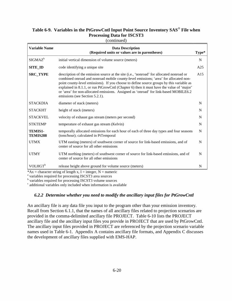
Table 6-9. Variables in the PtGrowCntl Input Point Source Inventory SAS® File when Processing Data for ISCST3
(continued)
6-20
Variable Name Data Description (Required units or values are in parentheses)
Type*
SIGMAZb initial vertical dimension of volume source (meters) N
SITE_ID code identifying a unique site A25
SRC_TYPE description of the emission source at the site (i.e., ‘nonroad’ for allocated nonroad or combined onroad and nonroad mobile county-level emissions; ‘area’ for allocated non-point county-level emissions). If you choose to define source groups by this variable as explained in 8.1.1, or run PtGrowCntl (Chapter 6) then it must have the value of ‘major’ or ‘area’ for non-allocated emissions. Assigned as ‘onroad’ for link-based MOBILE6.2 emissions (see Section 5.2.1).
A15
STACKDIA diameter of stack (meters) N
STACKHT height of stack (meters) N
STACKVEL velocity of exhaust gas stream (meters per second) N
STKTEMP temperature of exhaust gas stream (Kelvin) N
TEMIS1-TEMIS288
temporally allocated emissions for each hour of each of three day types and four seasons (tons/hour); calculated in PtTemporal
N
UTMX UTM easting (meters) of southwest corner of source for link-based emissions, and of center of source for all other emissions
N
UTMY UTM northing (meters) of southwest corner of source for link-based emissions, and of center of source for all other emissions
N
VOLHGTb release height above ground for volume source (meters) N *Ax = character string of length x, I = integer, N = numeric a variables required for processing ISCST3 area sources b variables required for processing ISCST3 volume sources c additional variables only included when information is available 6.2.2 Determine whether you need to modify the ancillary input files for PtGrowCntl An ancillary file is any data file you input to the program other than your emission inventory. Recall from Section 6.1.1, that the names of all ancillary files related to projection scenarios are provided in the comma-delimited ancillary file PROJECT. Table 6-10 lists the PROJECT ancillary file and the ancillary input files you provide in PROJECT that are used by PtGrowCntl. The ancillary input files provided in PROJECT are referenced by the projection scenario variable names used in Table 6-1. Appendix A contains ancillary file formats, and Appendix C discusses the development of ancillary files supplied with EMS-HAP.
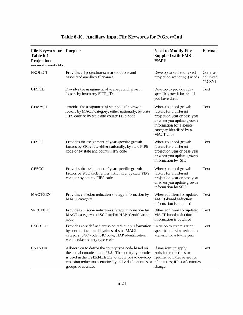
6-21
Table 6-10. Ancillary Input File Keywords for PtGrowCntl
File Keyword or Table 6-1 Projection scenario variable
Purpose Need to Modify Files Supplied with EMS-HAP?
Format
PROJECT Provides all projection-scenario options and associated ancillary filenames
Develop to suit your exact projection scenario(s) needs
Comma-delimited (*.CSV)
GFSITE Provides the assignment of year-specific growth factors by inventory SITE_ID
Develop to provide site-specific growth factors, if you have them
Text
GFMACT Provides the assignment of year-specific growth factors by MACT category, either nationally, by state FIPS code or by state and county FIPS code
When you need growth factors for a different projection year or base year or when you update growth information for a source category identified by a MACT code
Text
GFSIC Provides the assignment of year-specific growth factors by SIC code, either nationally, by state FIPS code or by state and county FIPS code
When you need growth factors for a different projection year or base year or when you update growth information by SIC
Text
GFSCC Provides the assignment of year-specific growth factors by SCC code, either nationally, by state FIPS code, or by county FIPS code
When you need growth factors for a different projection year or base year or when you update growth information by SCC
Text
MACTGEN Provides emission reduction strategy information by MACT category
When additional or updated MACT-based reduction information is obtained
Text
SPECFILE Provides emission reduction strategy information by MACT category and SCC and/or HAP identification code
When additional or updated MACT-based reduction information is obtained
Text
USERFILE Provides user-defined emission reduction information by user-defined combinations of site, MACT category, SCC code, SIC code, HAP identification code, and/or county type code
Develop to create a user-specific emission reduction scenario for a future year
Text
CNTYUR Allows you to define the county type code based on the actual counties in the U.S. The county-type code is used in the USERFILE file to allow you to develop emission reduction scenarios by individual counties or groups of counties
If you want to apply emission reductions to specific counties or groups of counties; if list of counties change
Text

6-22
6.2.3 Modify the growth factor input files (GFSITE, GFMACT, GFSIC, and GFSCC) Growth factors can come from numerous data sources such the Economic Growth Analysis System, version 4.08, (EGAS4.0) or future versions of the EGAS tool. MACT-based factors may not be provided by your growth factor tool; they are not produced by EGAS4.0. In this case, you can create them by mapping NAICS, SIC or SCC-based factors, depending upon which most appropriately matches, to specific MACT categories. Growth factors may also be developed through specific knowledge or economic studies of particular industries. Growth factors may be county-specific, state-specific or uniform across the nation. The MACT-based growth factor file indexes the factors by MACT and state and county FIPS code, whereas the SIC-based growth factor indexes it by SIC and state and county FIPS code. The state and county FIPS code can be used to control the geographic region over which the growth factor is to be applied: nationally, state-wide, or within a specific county. Assigning the state FIPS code and county FIPS code as shown in Table 6-11 does this.
Table 6-11. Regional Assignment of Growth Factors in the Growth Factor Files
Assignment of Growth Factor
State FIPS Code County FIPS Code
Nationally ‘00' ‘000'
State-wide specific state FIPS code ‘000'
County-wide specific state FIPS code specific county FIPS code
Note that any nationally applied growth factor will be superceded by a statewide growth factor, and any statewide growth factor will be superceded by a county-specific growth factor. The SIC-based growth factor file contains the same information as the MACT-based growth factor file, except that the growth factors are identified by SIC code. The growth factors are applied nationally, statewide, and within a specific county in the same way as in the MACT-based file. Note that if you assign growth factors by MACT category and by SIC, the SIC-based growth factors will not replace any assigned MACT-based growth factors. The SCC-based growth factor file (GFSCC) is set up differently than the MACT and SIC-based growth factor files. When examining the SCC-EGAS 4.0 output files, we found that there are generally dozens to hundreds of SCCs with similar growth factors. This is because SCCs are generally more detailed than the particular growth data from which they may be grown. Therefore, to reduce the size of the SCC growth factor file, the first part of the file contains only the SCC code and a cross-reference ‘indicator’ that links the SCC to a set of county, state, and/or national-level growth factors based on the indicator. The second part of the file contains the actual growth factors. See Appendix A for the file format.

6-23
Because you may want to use EMS-HAP to analyze a series of future years, you may have occasion to create a number of different MACT-based, SIC-based, and SCC-based growth factor files, with each separate version addressing a different base and projection year. You may also obtain site-specific growth factors that you can use to supercede all MACT, SIC, and SCC-based growth factors (see Table 6-2 in Section 6.1.2). By use of the PROJECT file, each run of PtGrowCntl can produce multiple projection scenario outputs (one scenario for each row of data in PROJECT). The base and projection years should be same within PROJECT each record (i.e., you wouldn’t use different projection years for the GFMACT and GFSIC files for the same projection scenario); also, the base year should be the same as the year of the emission inventory you input to EMS-HAP.
6.2.4 Modify the MACT-based emission reduction information files (MACTGEN and SPECFILE)
The general MACT reduction information file (MACTGEN) contains the list of MACT categories and the general reduction information described in Section 6.1.3. You will need to modify this file to account for updates to this information. Also, the MACT codes in the inventory undergo revisions periodically. The format for the general MACT reduction information file is provided in Appendix A. The specific MACT reduction information file (SPECFILE) contains reduction efficiencies for specific HAPs or specific processes within a MACT category as described in Section 6.1.3. Similarly, as discussed (above) for the MACTGEN file, you will need to modify this file to account for updates to the information and/or new MACT codes. The format for the specific MACT reduction information file is provided in Appendix A. If you need to apply reduction information at the site-level within a MACT category, you will need to use the user-defined emission reduction information file, USERFILE (see Section 6.2.5). It is important to note that all MACT categories included in the SPECFILE file must be included in the MACTGEN file. If not, the reduction information in the SPECFILE file for that MACT category will not be used. This is necessary because the compliance date from the MACTGEN file is used to determine whether or not the specific reduction information should be applied to the emissions for the specified projection year. The compliance date must be provided in the MACTGEN file. In cases where an emission inventory record is affected by more than one record in the specific MACT reduction information file, a specific order of precedence is followed. This order is presented in Table 6-3 (see Section 6.1.3). As an example, a reduction information record that specifies MACT code and 6-digit SCC will supercede a record that specifies MACT code and NTI_HAP.

6-24
6.2.5 Develop the user-defined emission reduction information files (USERFILE and CNTYUR)
The user-defined emission reduction information file (USERFILE) provides you flexibility to apply facility-specific emission reductions and/or create your own detailed reduction strategy information and preferences. If you want to apply your own emission reductions to the inventory, you will need to develop this file. The USERFILE file allows you to define emission reduction information by any combination of process and pollutant information, specified by the MACT code, SCC, SIC, and/or NTI_HAP variable. In addition, you can define any of this information for specific counties or groups of counties of your own creation (e.g., urban versus rural counties, counties in a specific MSA, or all counties within a state). Finally, you can define reduction information for a specific site using the SITE_ID variable. You can do this for the site alone or in various combinations with process and pollutant information, specified by the MACT code, SCC, SIC, and/or NTI_HAP variable. Section 6.1.4 describes how PtGrowCntl uses this file and the hierarchy of assigning the various strategies you may include in the file. You must modify the CNTYUR file if you choose a user-defined scenario that is specific to either a single county or a group of similar counties (e.g., all urban counties). You define specific counties or groups of counties for which you want to specify emission reduction information in PtGrowCntl, by populating the CNTYCODE variable in this file. All counties that you want to group together should have the same value for CNTYCODE. For example, if you want to develop a scenario for all urban counties, then you might use the code ‘URBAN’ for the CNTYCODE. You would then assign ‘URBAN’ to each urban county in the CNTYUR file. The CNTYUR file also contains 1999 county-level urban/rural designations to help you if you choose to use that as the basis of a reduction scenario. You must use the same value of CNTYCODE in the CNTYUR file as you use in the USERFILE file.
6.2.6 Prepare your batch file The batch file serves two purposes: (1) allows you to pass “keywords” such as file names and locations, program options, and run identifiers to the program, and (2) sets up the execute statement for the program. A sample batch file for PtGrowCntl for ASPEN emissions processing is shown in Figure B-10, of Appendix B. If processing emissions for ISCST3, simply change the keyword MODEL from ‘ASPEN’ to ‘ISC’ in the batch file. The best way to prepare your batch file is to copy one of the samples we provide and modify it to fit your needs. PtGrowCntl and CountyProc (Chapter 9) differ from all other EMS-HAP programs because, as discussed in 6.1.1 and shown in Table 6-1, they utilize an ancillary cross-reference file (PROJECT), which specifies all projection scenario-specific ancillary files and program options. Specify your keywords For PtGrowCntl, you need to specify filenames and parameters for keywords both in the batch file and the PROJECT file. The PROJECT file is a comma-delimited file that contains file

6-25
names and program options that instruct PtGrowCntl how to perform various projection scenarios. This is discussed in detail in Section 6.1.1; see in particular Table 6-1. You specify the filename for keyword PROJECT in the batch file. Table 6-12 shows you all the batch file keywords, and how to specify them for PtGrowCntl. Use the batch file keywords to locate all input and output emission files, and to name the emission input file and the prefix of the output file base name. The same batch file can be used for running PtGrowCntl for ASPEN or ISCST3. The only difference is the assignment of the keywords MODEL.
Table 6-12. Batch File Keywords in the PtGrowCntl for Either ASPEN or ISCST3
Keyword Description of Value Input Inventory Files IN_DATA Name of directory containing the input inventory SAS® file INSAS Input inventory SAS® file name, prefix of file name only Ancillary Files REFTEXT Name of directory containing ancillary files PROJECT File containing keywords for selecting PtGrowCntl functions, where each data record represents a
unique projection scenario (see Tables 6-1 and 6-13) Program Options MODEL ASPEN=process data for ASPEN model; ISC=process data for ISCST3 model Output files OUTDATA The output SAS® file directory OUTSAS When appended with PNAME from the PROJECT file (see Tables 6-1 and 6-13), produces the
base name of the output inventory SAS® file name, prefix only Edit the contents of the PROJECT file to set the number of projection scenarios and PtGrowCntl functions performed in each scenario. Table 6-13 provides the keywords in the PROJECT file, and Table 6-1 gives the file structure.

6-26
Table 6-13. PROJECT File Keywords for Selecting PtGrowCntl Functions
Keyword Description of Value Ancillary Files Names that you specify in the PROJECT file, prefix of filename only
Assign as ‘NONE’ or leave blank to prevent function GFSITE Growth factor file that provides growth factors by SITE_ID GFMACT MACT-based growth factors text file (e.g.; you might name these files with the form
gfXXmact_YY, where XX specifies base year and YY specifies projection year) GFSIC SIC-based growth factors text file (e.g.; you might name these files with the form gfXXsic_YY,
where XX specifies base year and YY specifies projection year) GFSCC SCC-based growth factors text file (e.g.; you might name these files with the form gfXXscc_YY,
where XX specifies base year and YY specifies projection year) MACTGEN General MACT-based emission reduction information text file SPECFILE Specific MACT-based emission reduction information text file USERFILE User-defined emission reduction information text file CNTYUR State/County FIPS code to county control code cross-reference text file Projection Scenario Options/ Parameters that you specify in the Project File YEARTYPE CALENDAR = Project Emissions beginning January 1 in the projected year
FISCAL = Project Emissions beginning October 1 in the year prior to the projected year GROWYEAR Year to which emissions are to be projected PNAME Parameter string that PtGrowCntl appends to the batch file keyword OUTSAS (see Table 6-12) to
produce the prefix of the projection scenario-specific output inventory SAS® file name You must include values for all keywords in your batch file. In the PROJECT file, you must provide either names, the word “NONE” or “” for the projection scenario filenames depending on whether or not you want to perform the particular growth/control function associated with that file. For example, if you do not wish to apply any growth factors for a projection scenario, you can either put “NONE,NONE,NONE,NONE” (or, “,,,,”) as the first four entries (representing file names for GFSITE, GFMACT, GFSIC, and GFSCC) for that scenario. Note, do not include the double quotes in the PROJECT file. Prepare the execute statement The last line in the batch file runs the PtGrowCntl program. In the sample batch file provided in Figure B-10 of Appendix B, you will see a line preceding the run line that creates a copy of the PtGrowCntl code having a unique name. It is this version of the program that is then executed in the last line. If you do this, the log and list files created by this run can be identified by this unique name. If you don’t do this and run the program under a general name, every run of PtGrowCntl will create a log and list file that will replace any existing files of the same name. You may find that you need to define a special area on your hard disk to use as workspace when running PtGrowCntl. In the sample batch file, a work directory is defined on the last line following the execution of PtGrowCntl. For example, the statement:

6-27
‘sas PtGrowCntl_062000.sas -work /data/work15’ assigns a assigns a SAS® work directory in the “/data/work15” directory. The directory you reference here must be created prior to running the program. 6.2.7 Execute PtGrowCntl There are two ways to execute the batch file. One way is to type ‘source’ and then the batch file name. Alternatively, first set the permission on the file to ‘execute.’ You do this by using the UNIX chmod command and adding the execute permission to yourself, as the owner of the file, to anyone in your user group, and/or to anyone on the system. For example, ‘chmod u+x PtGrowCntl.bat’ gives you permission to execute the batch file. Refer to your UNIX manual for setting other permissions. After you have set the file permission, you can execute the batch file by typing the file name on the command line, for example, ‘PtGrowCntl.bat’. 6.3 How Do I Know My Run of PtGrowCntl Was Successful? 6.3.1 Check your SAS® log file You need to review the output log file to check for errors or other flags indicating incorrect processing. This review should include searching the log files for occurrences of the strings “ERROR”, “WARNING”, “not found”, and “uninitialized”. These can indicate problems with input files or other errors. You can also look at the number of records in the input inventory file and compare it to the number of records in the output inventory file. The number of records should be the same in these two files. 6.3.2 Check your SAS® list file The list file created when PtGrowCntl is executed contains information to assist in quality assurance. This file can contain the information listed below, reported for each projection scenario you include in the PROJECT file. The contents of the list file from a specific run of PtGrowCntl depend on the functions you choose to have PtGrowCntl perform for each scenario.
C List of the general MACT emission reduction information (MACTGEN) records to be used considering the application control code and the projection year
C Summary of inventory records assigned general MACT (MACTGEN) reduction information
C List of specific MACT emission reduction information (SPECFILE) records to be used considering the application code
C List of duplicate records in SPECFILE file C List of SPECFILE file information not assigned to any records in the inventory C Summary of inventory records assigned SPECFILE information C List of user-defined emission reduction (USERFILE) information indicating which
records contain information that is to be used considering the application control code and the projection year

6-28
C List of state and county FIPS codes in the CNTYUR file that are not found in the inventory
C List of duplicate records in the USERFILE file C List of USERFILE information not assigned to a record in the inventory C Summary of inventory records USERFILE information C Summary of assigned growth factors and emission reduction information and the
resulting projected emissions
6.3.3 Check other output files from PtGrowCntl You should check for the existence of the output inventory file(s) named by keyword OUTSAS. This file will serve as the input to PtFinal_ASPEN or PtFinal_ISCST3, depending on the model you are using. If your projection included the use of any reduction strategies (MACT, user-defined, or both), the output inventory file will contain the variable CNTLCODE. This variable contains information about which reduction information (general MACT, specific MACT, and/or user-defined) was assigned to the emission record and how the information was combined for the assignment of the primary and additional control efficiencies. Reviewing the CNTLCODE variable can help confirm how your reduction strategies were used to project the emissions. If your projection included the use of growth factors, the output inventory file will contain the variable GFCODE. This variable contains information about what growth information (MACT, SIC or SCC) was assigned to the emission record.

7-1
CHAPTER 7
Point Source Processing The Final Format Program for ASPEN
(PtFinal_ASPEN) The flowchart below (Figure 7-1) shows how PtFinal_ASPEN fits into EMS-HAP’s point source processing for the ASPEN model. You don’t use this program if you are processing emissions for ISCST3. The point source inventory you input to PtFinal_ASPEN is either the output from PtTemporal (Chapter 5) or the output from PtGrowCntl (Chapter 6). You use the output from PtFinal_ASPEN as the input emission files for the ASPEN model.
Figure 7-1. Overview of PtFinal_ASPEN within EMS-HAP Point Source Processing
PtDataProc
PtModelProc
PtTemporal
PtGrowCntl
PtFinal_ASPEN
OR
Point source emissions
ASPEN point source emissions files

7-2
7.1 What is the function of PtFinal_ASPEN? The Final Format Program for ASPEN (PtFinal_ASPEN) creates the emission input files for the ASPEN model. PtFinal_ASPEN performs the functions listed below.
• PtFinal_ASPEN assigns ASPEN source groups used in the ASPEN model output • PtFinal_ASPEN converts temporally allocated emissions from tons/year to grams/second
for each of the eight 3-hour periods • PtFinal_ASPEN creates ASPEN input files, a SAS® file and an optional column
formatted text file
Figure 7-2 shows a flowchart of PtFinal_ASPEN. The keywords DOASCII and DOWRITE in the figure represent options you have in the particular of outputs PtFinal_ASPEN produces. Table 7-4 in Section 7.2.4 provides more information. The following sections describe the above bullets.

7-3
Reads keywordsBatch file containing keywords e.g. file names and locations, program
options
ASCII text point source emissions file (keyword ASCII)
PtFinal_ASPEN: MACRO FILEHEAD Reads reactivity class decay rate file. Creates ASPEN input emission files for each reactivity class. Writes header and reactivity decay rates to these files.
Reactivity class decay rate file (keyword DECAY)
PtFinal_ASPEN: MACRO GROUPSET Reads point source inventory file. Depending on program options, reads source group by MACT category file, source group by SCC file, and/or source by SIC file. Assigns source group as instructed by program options.
Source group by MACT category file (keyword MACTGRP)
Source group by SCC file (keyword SCCGRP)
Source group by SIC file (keyword SICGRP)
Point source inventory file (keyword INSAS)
PtFinal_ASPEN: MACRO ASCII2 Creates ASCII text version of data written to ASPEN input emission files. Converts 3-hr emission rates from tons/year to grams/sec if DOWRITE=0.
ASPEN input point source emission files reactivity classes 1 through 9
PtFinal_ASPEN: MACRO FILEBODY Converts 3-hr emission rates from tons/year to grams/sec. Writes data (grams/second) to ASPEN input emissions files for each reactivity class.
Point source inventory SAS dataset (keyword OUTSAS);
contains ASPEN-specific variables if batch file keywords are selected
Figure 7-2. PtFinal_ASPEN Flow Chart
If DOWRITE =1
If D
OW
RIT
E =0
an
d D
OA
SCII=
0
If D
OW
RIT
E = 0
an
d D
OA
S CII=
1
If DOASCII =0If
DO
ASC
I I =1

7-4
7.1.1 PtFinal_ASPEN assigns ASPEN source groups used in the ASPEN model output
The ASPEN model computes concentrations by source groups, which can be used to analyze the relative impacts of different types of emission sources. ASPEN can use up to 10 source groups. PtFinal_ASPEN can assign ASPEN source groups by the criteria listed below. You choose the method based on the keywords you specify in your batch file (see Table 7-4 in Section 7.2.4).
• source type: major, area or nonroad (variable SRC_TYPE) • MACT category code (variable MACT) • SCC (up to 10 digits allowed) • SIC
The assigned source group value (which can be 0 through 9) is stored in the variable named GROUP. When assigning the source group by SRC_TYPE, PtFinal_ASPEN makes the assignment as shown in Table 7-1.
Table 7-1. Assignment of Source Groups for ASPEN Model Using Source Type
Value of SRC_TYPE
Variable
Description Source Group Assignment
major major source of HAPs based on definition in Section 112 of Clean Air Acta
0
area area source of HAPs based on definition in Section 112 of Clean Air Actb
1
nonroad nonroad mobile source emissionsc 3 a “...any stationary source or group of stationary sources located within a contiguous area and under common control that emits or has the potential to emit considering controls, in the aggregate, 10 tons per year or more of any hazardous pollutant or 25 tons per year or more of any combination of hazardous air pollutants...” b “...any stationary source of hazardous air pollutants that is not a major source... shall not include motor vehicles or nonroad vehicles subject to regulation under title II...” c In point source processing, the most likely nonroad sources you would have in your point source inventory are allocated airport-related emissions such as aircraft emissions and airport support equipment emissions from COPAX (see Chapter 2) If you choose to assign the source group by the MACT category, the SCC, or the SIC, PtFinal_ASPEN uses the appropriate ancillary files represented by ancillary file keywords MACTGRP, SCCGRP, and/or SICGRP, respectively (see Table 7-5 for a full list of keywords). These files contain the group assignment value by code. See Section 7.2.3 for instructions on how to modify these files if you choose to assign your groups this way. Although you may choose several of the criteria listed above, PtFinal_ASPEN will not combine
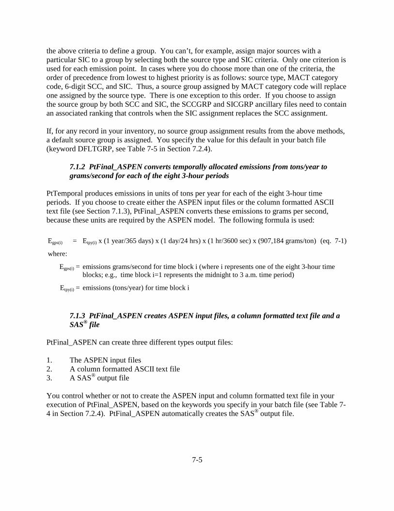
7-5
the above criteria to define a group. You can’t, for example, assign major sources with a particular SIC to a group by selecting both the source type and SIC criteria. Only one criterion is used for each emission point. In cases where you do choose more than one of the criteria, the order of precedence from lowest to highest priority is as follows: source type, MACT category code, 6-digit SCC, and SIC. Thus, a source group assigned by MACT category code will replace one assigned by the source type. There is one exception to this order. If you choose to assign the source group by both SCC and SIC, the SCCGRP and SICGRP ancillary files need to contain an associated ranking that controls when the SIC assignment replaces the SCC assignment. If, for any record in your inventory, no source group assignment results from the above methods, a default source group is assigned. You specify the value for this default in your batch file (keyword DFLTGRP, see Table 7-5 in Section 7.2.4).
7.1.2 PtFinal_ASPEN converts temporally allocated emissions from tons/year to grams/second for each of the eight 3-hour periods
PtTemporal produces emissions in units of tons per year for each of the eight 3-hour time periods. If you choose to create either the ASPEN input files or the column formatted ASCII text file (see Section 7.1.3), PtFinal_ASPEN converts these emissions to grams per second, because these units are required by the ASPEN model. The following formula is used: Egps(i) = Etpy(i) x (1 year/365 days) x (1 day/24 hrs) x (1 hr/3600 sec) x (907,184 grams/ton) (eq. 7-1)
where:
Egps(i) = emissions grams/second for time block i (where i represents one of the eight 3-hour time blocks; e.g., time block i=1 represents the midnight to 3 a.m. time period)
Etpy(i) = emissions (tons/year) for time block i
7.1.3 PtFinal_ASPEN creates ASPEN input files, a column formatted text file and a SAS® file
PtFinal_ASPEN can create three different types output files: 1. The ASPEN input files 2. A column formatted ASCII text file 3. A SAS® output file You control whether or not to create the ASPEN input and column formatted text file in your execution of PtFinal_ASPEN, based on the keywords you specify in your batch file (see Table 7-4 in Section 7.2.4). PtFinal_ASPEN automatically creates the SAS® output file.

7-6
ASPEN Input Files The ASPEN model requires emission data in the form of one ASCII text file for each of the nine possible reactivity/particulate size classes. Each file contains data for all pollutants having the same class. PtFinal_ASPEN creates all nine files in the appropriate format. (See Section 4.0 of the ASPEN User’s Guide1 for more details on the required format.) Each text file consists of a header and body. The elements of the header are:
$ A run identifier: You supply this in the batch file (keyword RUNID, see Table 7-5 in Section 7.2.4).
$ Species type: PtFinal_ASPEN sets this to 0 for gaseous species, 1 for fine particulates, and 2 for coarse particulates.
$ Wet and dry deposition codes: PtFinal_ASPEN sets these to 0 for particulates and 1 for gaseous species. These values tell ASPEN whether to invoke the deposition algorithm for particulates (ASPEN does not perform deposition for gases).
$ Decay coefficients associated with the reactivity class: PtFinal_ASPEN determines these from the DECAY ancillary file based on the value of the REACT variable (discussed in detail in Chapter 4, Section 4.2.3). This file contains a set of coefficients for each of the nine reactivity/particulate size classes.
The file body contains source information such as latitude and longitude, the source group, source characteristics such as stack height, building width, and vent type, and the emissions for each of eight 3-hour periods for each pollutant (of the appropriate reactivity/particulate size class) emitted from the stack. PtFinal_ASPEN names the nine ASPEN input files in the form ‘OUTCODE.rREACT.inp’ where OUTCODE is the file identifier keyword you provide in the batch file (see Table 7-5 in Section 7.2.4), and REACT is the reactivity/particulate size class (a number between 1 and 9, inclusive). An example file name is ‘Pt96.US.D121599.r1.inp’ where OUTCODE is ‘Pt96.US.D121599' and REACT is ‘1'. Column-Formatted ASCII File PtFinal_ASPEN can create a single column-formatted ASCII text file containing data written to the ASPEN input emission files. This file can provide easy access to the data for quality assurance purposes. You specify the prefix name of this file in your batch file (keyword ASCII, see Table 7-5 in Section 7.2.4); the suffix is ‘.txt’. Table 7-7 in Section 7.3.3 shows the format of this file. SAS® Output File PtFinal_ASPEN automatically creates an output SAS® inventory file. This file contains the same data as in the input SAS® inventory file with the following exceptions:

7-7
$ The source group variable (GROUP), and possibly some ASPEN-specific variables (see Table 7-6 in Section 7.3.3), have been added.
$ The units of the temporally allocated emissions have been converted to grams/second
(except for the unlikely event that you chose to create neither the ASPEN input nor the column-formatted ASCII files)
You specify the name of this file in your batch file (keyword OUTSAS, see Table 7-5 in Section 7.2.4). 7.2 How do I run PtFinal_ASPEN? 7.2.1 Prepare your point source inventory for input into PtFinal_ASPEN The point source inventory you use for input into PtFinal_ASPEN can be the output from either PtTemporal (see Chapter 5) or PtGrowCntl (see Chapter 6). The inventory produced by either of these programs will meet all requirements and will contain the variables listed in Table 7-2 with some exceptions. If the output from PtTemporal is used, the file will not include the control variables created in PtGrowCntl. The file may also contain additional variables such as the diagnostic flag variables (LFLAG, FIPFLAG, etc.) created by PtDataProc depending on the options you chose for the windowing function in PtDataProc (see Section 3.1.3).

7-8
Table 7-2. Variables in the PtFinal_ASPEN Input Point Source Inventory SAS® File Variable Name Data Description
(Required units or values are in parentheses) Type*
ADDNEFF a reduction (%) for new sources to be applied in addition to primary reductions; assigned in PtGrowCntl (see Section 6.1.4)
N
ADDXEFF a reduction (%) for existing sources to be applied in addition to primary reductions; assigned in PtGrowCntl (see Section 6.1.4)
N
ADD_RATE a percentage of emissions attributable to new sources for the purpose of applying additional reductions; assigned in PtGrowCntl (see Section 6.1.4)
N
BLDH building height (meters) (5 for horizontal stacks, 0 for all other stacks); assigned in PtModelProc (see Section 4.1.3)
N
BLDW building width (meters) (5 for horizontal stacks, 0 for all other stacks); assigned in PtModelProc (see Section 4.1.3)
N
CNTL_EFF baseline reduction efficiency, expressed as a percentage N
CNTLCODE a control code indicating the reductions applied to emissions; assigned in PtGrowCntl A100
EMIS baseline pollutant emissions value (tons/year) N
EMRELPID code identifying a unique emission point within a site A50
EMRELPTY physical configuration code of release point (01=fugitive; 02=vertical stack; 03=horizontal stack, 04=goose neck, 05=vertical with rain cap, 06=downward-facing vent, 99=other, AP= allocated to point during COPAX –i.e., aircraft)
A4
EXISTEFF a primary percent reduction for existing sources; assigned in PtGrowCntl (see Section 6.1.4)
N
FIPS 5-digit FIPS code (state and county combined) A5
GFa growth factor; assigned in PtGrowCntl (see Section 6.1.1) N
GFCODEa growth factor application method; assigned in PtGrowCntl A7
IBLDG building code (1 for horizontal stacks, 0 for all other stacks); assigned in PtModelProc (see Section 4.1.3)
A1
IVENT vent type (0 for stacked sources, 1 for non-stacked sources); assigned in PtModelProc (see Section 4.1.3)
A1
LAT latitude (decimal degrees) N
LON longitude (negative decimal degrees for Western Hemisphere) N
MACT MACT code A7
NEW_EFF a primary percent reduction for new sources; assigned in PtGrowCntl (see Section 6.1.4)
N

Table 7-2. Variables in the PtFinal_ASPEN Input Point Source Inventory… (continued)
7-9
Variable Name Data Description (Required units or values are in parentheses)
Type*
NEW_RATE a percentage of emissions attributable to new sources for the purpose of applying primary reductions; assigned in PtGrowCntl (see Section 6.1.4)
N
NTI_HAP code identifying HAP on the Clean Air Act HAP list; assigned in PtModelProc (see Section 4.1.1)
A3
REACT pollutant reactivity/particulate size class (1-9); assigned in PtModelProc (see Section 4.1.1)
N
REPLACEa user-defined reduction flag (R=replace MACT-based reductions with user-defined reductions; A=apply user-defined reductions in addition to the primary MACT-based reductions); assigned in PtGrowCntl (see Section 6.1.4)
A1
SAROAD unique pollutant-group code; assigned in PtModelProc (see Section 4.1.1) A10
SAROADDC descriptive name for the SAROAD; assigned in PtModelProc (see Section 4.1.1) A50
SCC EPA source category code identifying the process A10
SCC_AMS SCC or AMS code from the temporal allocation factor file identifying the temporal profile used; assigned in PtTemporal
A10
SIC Standard Industrial Classification (SIC) code for the site A4
SITE_ID code identifying a unique site A25
SRC_TYPE description of the emission source at the site. If you choose to define source groups by this variable as explained in 7.1.1, or run PtGrowCntl (Chapter 6) then it must have the value of ‘major’ or ‘area’ for non-allocated emissions. For allocated emissions: ‘nonroad’ for allocated nonroad or combined onroad and nonroad county-level emissions; ‘area’ for allocated non-point county-level emissions
A15
STACKDIA diameter of stack (meters) N
STACKHT height of stack (meters) N
STACKVEL velocity of exhaust gas stream (meters per second) N
STKTEMP temperature of exhaust gas stream (Kelvin) N
TAFS1-TAFS8 temporal factors for the eight 3-hour periods of an average day; assigned in PtTemporal N
TEMIS1-TEMIS8 temporally allocated emissions for the eight 3-hour periods of an average day (tons/year); calculated in PtTemporal, unless emission projections were done in which case, values represent temporally allocated projected emissions calculated in PtGrowCntl
N
UFLAG urban/rural dispersion flag (1 for urban, 2 for rural); assigned in PtModelProc (see Section 4.1.2)
N
*Ax = character string of length x, I = integer, N = numeric a variable present only if you run the optional Growth and Control Program, PtGrowCntl (Chapter 6)

7-10
7.2.2 Determine whether you need to modify the ancillary input files for PtFinal_ASPEN
An ancillary file is any data file you input to the program other than your emission inventory. Table 7-3 lists the ancillary input files required for PtFinal_ASPEN and when you may need to modify them. Appendix A contains ancillary file formats, and Appendix C discusses the development of ancillary files supplied with EMS-HAP.
Table 7-3. Ancillary Input File Keywords for PtFinal_ASPEN
File Keyword Purpose Need to Modify the file supplied with EMS-HAP ?
Format
MACTGRP Provides the assignment of source groups by MACT code
If you want to make source group assignments by MACT code
Text
SCCGRP Provides the assignment of source groups by 6-digit SCC and a rank code used to determine if the source group can be replaced by a SIC-based source group
If you want to make source group assignments by SCC code
Text
SICGRP Provides the assignment of source groups by SIC and a rank code used to determine if the source group can replace a SCC-based source group
If you want to make source group assignments by SIC code
Text
DECAY Provides decay coefficients for 6 stability classes for the eight 3-hour time periods for up to 9 reactivity/particulate classes
No Text
7.2.3 Modify the source group assignment files (ancillary file keywords MACTGRP, SCCGRP, and SICGRP)
The ASPEN model output presents data for each pollutant (SAROAD) by census tract and by source group. The source group assignment you make in PtFinal_ASPEN will determine how ASPEN will group the concentration estimates. You can control this assignment based on the source type using the SRC_TYPE variable (as was discussed in 7.1.1) and/or by using any one of the three ASPEN source group assignment files. The ancillary file MACTGRP refers to a simple text file that has a MACT code followed by a source group code (number between 0 and 9, inclusive). To modify it, put the same group code next to each MACT code that you want in the same group. If you choose to use this file in combination with either of the other two files, it is important to remember that a MACT code-based assignment will automatically replace a source type-based assignment and will automatically be replaced by either an SCC-based or SIC-based assignment.

7-11
If you want to use both SCC-based assignments and SIC-based assignments, you can control whether or not the SIC-based assignment replaces the SCC-based assignment by setting the rank field in each file. These files contain the SCC or SIC code followed by the source group, followed by the rank. If an inventory record contains both SCC and SIC codes, the SCC assignment is made first. If an assignment can also be made by SIC, the SIC-based assignment will only replace the SCC-based assignment if the SIC rank is lower than the SCC rank (e.g., an SIC rank of 1 and a SCC rank of 3 will result in the SIC-based assignment replacing the SCC-based assignment of the source group). 7.2.4 Prepare your batch file The batch file serves two purposes: (1) allows you to pass “keywords” such as file names and locations, program options and run identifiers to the program, and (2) sets up the execute statement for the program. A sample batch file for PtFinal_ASPEN is shown in Figure B-11 of Appendix B. The best way to prepare your batch file is to copy the sample we provide and modify it to fit your needs. Specify your keywords Table 7-4 shows you how to specify keywords to select PtFinal_ASPEN functions.
Table 7-4. Keywords for Selecting PtFinal_ASPEN Functions
PtFinal_ASPEN Function Keyword (values provided cause function to be performed)
Process data for ASPEN model MODEL = ASPEN
Assign ASPEN source groups
by source type DOSOURCE = 1
by MACT code DOMACT = 1
by SCC DOSCC = 1
by SIC DOSIC = 1
Create ASPEN input files DOWRITE = 1
Create single text-formatted file DOASCII = 1 Table 7-5 describes all of the keywords required in the batch file. In addition to supplying all input and output file names and directories and program options, you must also supply additional input data (see “Additional Input Data” section in Table 7-5). You must supply a value for keyword ITYPE, which tells ASPEN whether your sources are point or pseudopoint sources. Always set the keyword ITYPE to 0 (which signifies point source).

7-12
Table 7-5. Keywords in the PtFinal_ASPEN Batch File Keyword Description of Value Input Inventory Files IN_DATA Name of directory containing the input inventory SAS® file INSAS Input inventory SAS® file name, prefix of file name only Ancillary Files REFFILES Name of directory containing the ancillary files MACTGRP MACT code to source group correspondence text file, prefix of file name only SCCGRP SCC code to source group correspondence text file, prefix of file name only SICGRP SIC code to source group correspondence text file, prefix of file name only DECAY Reactivity class decay coefficients for 6 stability classes for eight 3-hour time periods text file,
prefix of file name only Program Options (also see Table 7-4) MODEL ASPEN = process data for the ASPEN model DOSOURCE 1= assign source group by source type; 0=don’t assign by source type DOMACT 1=assign source group by MACT category code; 0=don’t assign by MACT DOSCC 1=assign source group by SCC code; 0=don’t assign by SCC DOSIC 1=assign source group by SIC code; 0=don’t assign by SIC DOWRITE 1=create ASPEN input emission files; 0=don’t create ASPEN input files DOASCII 1=create column-formatted ASCII text output file; 0=don’t create column-formatted ASCII
text output file Additional Input Data DFLTGRP Default source group (must be an integer between 0 and 9, inclusive) OUTCODE File identifier included in name of ASPEN input emission files (limit of 10 characters is
recommended. Additional characters will be truncated from the file header, not the file name) ITYPE ASPEN Source type (0 for point sources) RUNID Run identifier included in ASPEN input emission file header (limit of 25 characters is
recommended. Additional characters will be truncated) Output files OUTDATA Output SAS® file directory OUTSAS Output inventory SAS® file name, prefix of file name only OUTFILES Output ASPEN emission files directory ASCIIFILE Output ASCII text file directory ASCII Column-formatted ASCII text file name, prefix of file name only
You should include all batch file keywords even if they are related to a function that you don’t select to perform. For example, if you set keyword DOMACT to 0 (zero), you still need the ancillary file keyword MACTGRP in your batch file; however, the value of this keyword may be blank. The value provided in this circumstance does not need to represent an actual file name; it is merely a placeholder value for the keyword.

7-13
Prepare the execute statement The last line in the batch file runs the PtFinal_ASPEN program. In the sample batch file provided in Figure B-11 of Appendix B, you will see a line preceding the run line that creates a copy of the PtFinal_ASPEN code with a unique name. It is this version of the program that is then executed in the last line. If you do this, the log and list files created by this run can be identified by this unique name. If you don’t do this and run the program under a general name, every run of PtFinal_ASPEN will create a log and list file that will replace any existing files of the same name. You may find that you need to assign a special area on your hard disk to use as workspace when running PtFinal_ASPEN. In the sample batch file, a work directory is defined on the last line following the execution of PtFinal_ASPEN. For example, the command ‘sas PtFinal_ASPEN_062000.sas -work /data/work15/dyl/’ assigns a SAS® work directory in the “/data/work1/dyl” directory. The directory you reference must be created prior to running the program. 7.2.5 Execute PtFinal_ASPEN There are two ways to execute the batch file. One way is to type ‘source’ and then the batch file name. Alternatively, first set the permission on the file to ‘execute.’ You do this by using the UNIX chmod command and adding the execute permission to yourself, as the owner of the file, to anyone in your user group, and/or to anyone on the system. For example, ‘chmod u+x PtFinal_ASPEN.bat’ gives you permission to execute the batch file. Refer to your UNIX manual for setting other permissions. After you have set the file permission, you can execute the batch file by typing the file name on the command line, for example, ‘PtFinal_ASPEN.bat’. 7.3 How Do I Know My Run of PtFinal_ASPEN Was Successful? 7.3.1 Check your SAS® log file You need to review the output log file to check for errors or other flags indicating incorrect processing. This review should include searching the log files for occurrences of the strings “ERROR”, “WARNING”, “not found”, and “uninitialized”. These can indicate problems with input files or other errors. You can look at the number of records in the input inventory file and compare it to the number of records in the output SAS® inventory file. The number of records should be the same in these two files.

7-14
7.3.2 Check your SAS® list file This file lists each unique combination of source type (SRC_TYPE), MACT, SCC, and SIC code and the resulting source group (GROUP) assigned by PtFinal_ASPEN. You can check these assignments to see that they are what you intended. If you assigned the GROUP by SRC_TYPE, you should check this list to make sure that there are no missing source types. Note that this list could be large, depending on the number of combinations of different codes in your inventory. This file also shows the results of the SAS® CONTENTS procedure on the output SAS® inventory file. 7.3.3 Check other output files from PtFinal_ASPEN PtFinal_ASPEN can create several different output files. It automatically creates an output SAS® inventory file, named by keyword OUTSAS. This file contains the same data as in the input SAS® inventory file and additional data that depends on how you set the keywords DOASCII and DOWRITE in the batch file (see Table 7-4 in Section 7.2.4). Table 7-6 lists the variables that can be added to the output point source inventory. The temporally allocated emission values are also converted from tons/year to grams/sec (see Section 7.1.2) if you choose to create the either the ASPEN input or column formatted ASCII files (i.e., either keyword DOWRITE or keyword DOASCII=1).
Table 7-6. Variables Added to Input Inventory in Creating the PtFinal_ASPEN Output Point Source Inventory SAS® File
Variable Name Data Description (Required units or values are in parentheses) Type*
GROUP Emissions source group written to the ASPEN input file; assigned in PtFinal_ASPEN A1
ITYPE ASPEN source type written to the ASPEN input file (0=point; 3= pseudopoint. Should be “0" for all point sources); assigned if batch file keywords DOASCII or DOWRITE = 1
A1
PLANTID Plant ID variable written to the ASPEN input file (first 10 characters of EMS-HAP SITE_ID); assigned if batch file keywords DOASCII or DOWRITE = 1
A10
STACKID Stack ID variable written to the ASPEN input file (last five characters of the EMRELPID variable); assigned if batch file keywords DOASCII or DOWRITE = 1
A5
*Ax = character string of length x, If you set the DOWRITE keyword to 1 (one), PtFinal_ASPEN will create nine ASPEN input emission files, one for each possible reactivity class. You should check that all nine files were created and that emission data are included only in those files representing reactivities/particulate size classes for which you know your inventory has emission data. You may also want to check the header of the files for the decay rate information. If you set the keyword DOASCII to 1 (one), PtFinal_ASPEN will create a single column formatted ASCII file, which can be helpful in checking the quality of the ASPEN input emission data. Table 7-7 lists the variables in this file.

7-15
Table 7-7. PtFinal_ASPEN Output ASCII File Variables Variables and Data Description (Units or values are in parentheses) Type* FIPS: 5-digit FIPS code; state and county combined A5
PLANT_ID: ASPEN plant ID (first 10 characters of EMS-HAP SITE_ID) A10
LON: point source longitude (negative decimal degrees for Western Hemisphere ) 10.5
LAT: point source latitude (decimal degrees) 8.5
ITYPE: ASPEN source type, 0 for point, 3 for pseudopoint (0) A1
UFLAG: urban/rural dispersion flag (1 for urban, 2 for rural) 1.0
STACKID: ASPEN Stack ID (last 5 characters of EMS-HAP EMRELPID) A5
STACKHT: height of stack (meters) 10.4
STACKDIA: diameter of stack (meters) 10.4
STACKVEL: velocity of exhaust gas stream (meters per second) 10.4
STKTEMP: temperature of exhaust gas stream (Kelvin) 10.2
SAROAD: unique pollutant-group code A5
GROUP: ASPEN source group (integer between 0 and 9, inclusive) A1
TEMISA1: Emissions rate (grams/second) for the first 3-hour time period E10.
TEMISA2: Emissions rate, time period 2 E10.
TEMISA3: Emissions rate, time period 3 E10.
TEMISA4: Emissions rate, time period 4 E10.
TEMISA5: Emissions rate, time period 5 E10.
TEMISA6: Emissions rate, time period 6 E10.
TEMISA7: Emissions rate, time period 7 E10.
TEMISA8: Emissions rate, time period 8 E10.
SITE_ID: Identifies a unique site (same as EMS-HAP SITE_ID) A25
* Ax = character string of length x, x.y = numeric format with y places right of decimal, Ex. = exponential

7-16
This page intentionally blank

8-1
CHAPTER 8
Point Source Processing The Final Format Program for ISCST3
(PtFinal_ISCST3) The flowchart below (Figure 8-1) shows how PtFinal_ISCST3 fits into EMS-HAP’s point source processing for the ISCST3 model. You don’t use this program if you are processing emissions for ASPEN. The point source inventory you input to PtFinal_ISCST3 is either the output from PtTemporal (Chapter 5) or the output from PtGrowCntl (Chapter 6). You use the output from PtFinal_ISCST3 as the source (SO) pathway section of the ISCST3 run stream for running the ISCST3 model.
Figure 8-1. Overview of PtFinal_ISCST3 within EMS-HAP Point Source Processing
PtDataProc
PtModelProc
PtTemporal
PtGrowCntl
PtFinal_ISCST3
OR
Point source emissions
ISCST3 SO pathway of run stream section for ISCST3 point, volume,
and area sources

8-2
8.1 What is the function of PtFinal_ISCST3? The Final Format Program for ISCST3 (PtFinal_ISCST3) creates the SO pathway section of the ISCST3 run stream. PtFinal_ISCST3 performs the functions listed below. C PtFinal_ISCST3 assigns source groups used in the ISCST3 model output C PtFinal_ISCST3 assigns default release parameters in order to model fugitive sources and
horizontal stacks as ISCST3 volume sources C PtFinal_ISCST3 assigns available particulate size and gas deposition data by pollutant or by
combination of SCC and pollutant C PtFinal_ISCST3 removes emission sources outside your modeling domain C PtFinal_ISCST3 assigns available emission source elevation data C PtFinal_ISCST3 assigns source identification codes needed for the ISCST3 SO pathway
section files C PtFinal_ISCST3 adjusts UTM coordinates of ISCST3 area emission sources from the center
of the source to its southwest corner C PtFinal_ISCST3 converts temporally allocated emissions from tons/hour to the necessary
units for each source for each of the 288 emission rates C PtFinal_ISCST3 creates SO pathway section of the ISCST3 run stream and include files Figure 8-2 shows a flowchart of PtFinal_ISCST3. The following sections describe the above bullets.

8-3
Reads keywordsBatch file containing keywords e.g., file names and locations, program
options
PtFinal_ISCST3: MACRO MERGASD Reads default gas deposition parameter file and assigns to emissions by pollutant.
Default gas deposition parameter file (keyword DEFGAS)
PtFinal_ISCST3: MACRO GROUPSET Reads point source inventory file. Depending on program options, reads source group by MACT category file, source group by SCC file, and/or source by SIC file and assigns source group to emission records.
Source group by MACT category file (keyword MACTGRP)
Source group by SCC file (keyword SCCGRP)
Source group by SIC file (keyword SICGRP)
Point source inventory file (keyword INSAS)
PtFinal_ISCST3: MACRO MERGELEV Reads grid cell elevation file and assigns elevation data to emissions by grid cell or census tract.
PtFinal_ISCST3: MACRO MERGPART Reads pollutant-level particle size distribution file and assigns to emissions by pollutant (SAROAD variable). Reads SCC-level particle size distribution file and assigns to emissions by SAROAD and SCC.
SCC-level particle size distribution file
(keyword SCCPART)
Pollutant-level particle size distribution file
(keyword DEFPART)
Grid cell or census tract elevation file (keyword ELEVDAT)
PtFinal_ISCST3: MACRO SOPATH Creates SO pathway of ISCST3 run stream. Creates all ISCST3 SO pathway include files. Converts emissions from tons/hour to appropriate units (grams/sec or grams/secxsquare meter).
PtFinal_ISCST3: MACRO FUGDEF Assigns default release parameters to fugitive sources and horizontal stacks in order to model these as ISCST3 volume sources.
PtFinal_ISCST3: MACRO GRIDCELL Determines grid cell for each source and retains only sources within modeling domain.
Figure 8-2 PtFinal_ISCST3 Flowchart
SO Pathway of ISCST3 Run Stream
SO Pathway include files

8-4
8.1.1 PtFinal_ISCST3 assigns source groups used in the ISCST3 model output The ISCST3 model can compute pollutant concentrations at the receptors by source groups. This information can then be used to analyze the relative impacts of different types of emission sources. For example, ISCST3 can output concentrations from dry cleaning sources separately from onroad mobile sources. This source group assignment is also incorporated into a sequential source identification code (discussed in 8.1.6) that PtFinal_ISCST3 assigns to each source for use in the ISCST3 model. ISCST3 can use up to 100 source groups. PtFinal_ISCST3 can assign source groups by the criteria listed below. You choose the method based on the keywords you specify in your batch file (see Table 8-9 in Section 8.2.5). $ source type (variable SRC_TYPE) $ MACT category code (variable MACT) $ SCC $ SIC The assigned source group value, which can be 00 through 99, is stored in the variable named GROUP. When assigning the source group by source type, PtFinal_ISCST3 makes the assignment as shown in Table 8-1.
Table 8-1. Assignment of Source Groups for the ISCST3 Model
Value of SRC_TYPE Variable
Description Source Group Assignment
major major source of HAPs based on definition in Section 112 of Clean Air Acta.
00
area area source of HAPs based on definition in Section 112 of Clean Air Actb.
01
onroad onroad mobile source emissions. Note that this SRC_TYPE will not be in your inventory unless you have appended the seasonal-hourly link based emissions in your inventory at the PtTemporal step (see Chapter 5).
02
nonroad nonroad mobile source emissions (for example: allocated aircraft emissions incorporated into the point source inventory through running COPAX).
03
a “...any stationary source or group of stationary sources located within a contiguous area and under common control that emits or has the potential to emit considering controls, in the aggregate, 10 tons per year or more of any hazardous pollutant or 25 tons per year or more of any combination of hazardous air pollutants...” b “...any stationary source of hazardous air pollutants that is not a major source... shall not include motor vehicles or nonroad vehicles subject to regulation under title II…”

8-5
If you choose to assign the source group by the MACT category, the SCC, or the SIC, PtFinal_ISCST3 uses the appropriate ancillary files represented by ancillary file keywords MACTGRP, SCCGRP, and/or SICGRP, respectively. These files contain the group assignment value by code. See Section 8.2.3 for instructions on how to modify these files if you choose to assign your groups this way. Although you may choose several of the criteria listed above, PtFinal_ISCST3 will not combine the above criteria to define a group. You can’t, for example, assign major sources with a particular SIC to a group by selecting both the source type and SIC criteria. Only one criterion is used for each inventory record. In cases where you do choose more than one of the criteria, the order of precedence from lowest to highest priority is as follows: source type, MACT code, SCC, and SIC. For example, a source group assigned by MACT code will replace one assigned by the source type. There is one exception to this order. If you choose to assign the source group by both SCC and SIC, the SCCGRP and SICGRP ancillary files contain an associated ranking that controls when the SIC assignment replaces the SCC assignment. See Section 8.2.3 for details. If no source group assignment is made by the above methods for any record in your inventory, a default source group is assigned. You specify the value for this default in your batch file (keyword DFLTGRP, see Table 8-10 in Section 8.2.5).
8.1.2 PtFinal_ISCST3 assigns default release parameters in order to model fugitive sources and horizontal stacks as ISCST3 volume sources
The ISCST3 model can process three types of EMS-HAP point sources located at specific coordinates: ISCST3 point sources, ISCST3 volume sources, and ISCST3 area sources. An ISCST3 point source is used to model discrete emission stacks and vents; we expect that the majority of your point source inventory will consist of this type of source. An ISCST3 volume source is used to model emission releases from various industrial sources, such as building roof monitors, multiple vents, and conveyor belts. An ISCST3 area source is used to model low level or ground level emission releases with no plume rise, such as storage piles, slag dumps, lagoons, landfills, airports, or onroad mobile segments. You can include ISCST3 volume and ISCST3 area sources in the point source inventory you input to EMS-HAP by including the variables required to describe these sources (see Table 3-7 in Section 3.2.1). Even if you don’t include ISCST3 volume sources in your inventory, PtFinal_ISCST3 assigns certain emission sources in your point source inventory, based on the emission release type (variable EMRELPTY), to be modeled as ISCST3 volume sources. These are fugitive sources (EMRELPTY=01) and horizontal sources (EMRELPTY=03), which are typically included in point source inventories, but we believe would be best modeled as ISCST3 volume sources rather than as ISCST3 point sources. For these release types in your inventory, PtFinal_ISCST3 assigns default ISCST3 volume source release parameters as shown in Table 8-2. Note, release height (VOLHGT) is assigned the source stack height if it is valid (nonzero and non-missing); otherwise, volume release height is defaulted. This assignment does not affect any ISCST3 volume or ISCST3 area sources you include in the inventory. PtFinal_ISCST3 also assigns the

8-6
ISCTYPE variable to the value ‘iscpoint’ to all sources not identified as either ISCST3 volume or ISCST3 area sources.
Table 8-2. Default ISCST3 Volume Source Release Parameters Assigned to Fugitive and Horizontal Emission Release Types
Variable Name Release Parameter Assigned Value
ISCTYPE ISCST3 source type ‘iscvolume’
VOLHGT Release height (meters) value of STACKHT variable, *
SIGMAX Initial lateral dimension of the volume 1.5 SIGMAZ Initial vertical dimension of the volume 1.5
* if stack height is zero or missing
8.1.3 PtFinal_ISCST3 assigns available particulate size and gas deposition data by pollutant or by combination of SCC and pollutant
The ISCST3 model includes several different algorithms for deposition, some of which require information in addition to the emission inventory data. The type of deposition and the additional information required is summarized in Table 8-3.
Table 8-3. ISCST3 Deposition Algorithms and Required Information
Type of Deposition Additional Information Required Specificity of Information
Gravitational settling and removal of particulates in the plume by dry deposition
Emission source particle size distribution parameters (particle diameter, mass fraction, and particle density) for up to 10 fractions
by SAROAD or SAROAD and SCC
Scavenging and removal of particles by wet deposition
Liquid and ice scavenging coefficients for up to 10 fractions
by SAROAD or SAROAD and SCC
Dry deposition and removal of gaseous pollutants
Molecular diffusivity, solubility enhancement factor, reactivity parameter, mesophyll resistence term, and Henry's Law coefficient
by SAROAD
Depending on which, if any, of these deposition algorithms you will be using when running the ISCST3 model, you need to provide the appropriate information by using one of three ancillary files. Ancillary file DEFGAS contains the gas deposition parameters and the liquid scavenging coefficients by pollutant (as identified by the SAROAD variable). Ancillary file DEFPART contains the particle size distribution information, and, if necessary, the liquid and ice scavenging coefficients by pollutant. Ancillary file SCCPART contains this same type of information, but by both the pollutant (SAROAD code) and the SCC code.

8-7
You control how the particle size distribution file and the gas deposition file are used in PtFinal_ISCST3 through the program options you specify in the batch file (see Table 8-9 in Section 8.2.5). If you instruct PtFinal_ISCST3 to read scavenging coefficients by setting the keyword SCAVENG to 1, then these coefficients will be read from both the gas deposition and particle size distribution files. 8.1.4 PtFinal_ISCST3 removes emission sources outside your modeling domain PtFinal_ISCST3 determines the grid cell or census tract with the nearest tract centroid for each point source as discussed below. Note that for the tract approach, PtFinal_ISCST3 finds the tract having the shortest distance between its centroid and the point; this is not necessarily the tract containing the point source. PtFinal_ISCST3 windows the inventory to exclude any records in grid cells or census tracts that are outside of the modeling domain; PtFinal_ISCST3 drops these records from the inventory. Under the grid cell approach, the first row and column delineate the southern and western extent of the domain. Grid cells are outside the domain if they have a column or row greater than the maximum column and row for the domain, or, if they are less than 1. When using the census tract approach, sources south or west of the domain origin specified in the batch file (X_ORIG and Y_ORIG) are removed. If you want other sources removed, you must remove them yourself, preferably before processing in EMS-HAP. PtFinal_ISCST3 computes the modeling grid cell of each emission source in your inventory using equations 8-1 through 8-3, below, and the information you supply in your batch file (Section 8.2.5) that describes your modeling grid. Table 8-4 summarizes this information. If using the census tract approach, PtFinal_ISCST3 assigns the census tract using information from the tract information file (ancillary file keyword TRACTINF). PtFinal_ISCST3 determines the tract with the shortest distance between the tract centroid and the emission source. For this approach, it is important that the batch keyword REF_ZONE be set to the UTM zone of your domain because the coordinates of the tract centroids in TRACTINF must be converted from latitudes and longitudes to UTM coordinates. The UTM zone must be the same as the UTM zone specified in PtDataProc (see Ch. 3, Section 3.1.1) to ensure accurate coordinate transformation.
Table 8-4. Modeling Grid Information Required by PtFinal_ISCST3 to Assign Grid Cell When Using Grid Cell Approach
Modeling Grid Information Batch File Keyword
UTM easting coordinate of grid origin (meters) X_ORIG
UTM northing coordinate of grid origin (meters) Y_ORIG
Grid cell size (meters) CELLSIZE
Number of grid columns MAXCOL
Number of grid rows MAXROW

8-8
The grid cell column, row, and cell number are computed from the equations given below.
COL = INT((UTMX - X_ORIG)/(CELLSIZE)) + 1 (Eq. 8-1)
ROW = INT((UTMY - Y_ORIG)/(CELLSIZE)) + 1 (Eq. 8-2)
CELL = (COL x 1000) + ROW (Eq. 8-3)
Where:
INT = integer function; the remainder is dropped. For example, if UTMX = 224500 and X_ORIG = 210000 and CELLSIZE = 1000, then COL equals INT(14.5) = 14
COL = modeling domain grid column number
UTMX = UTM easting coordinate (meters)
ROW = modeling domain grid row number
UTMY = UTM northing coordinate (meters)
CELL = modeling domain grid cell number
PtFinal_ISCST3 assigns the variables that define the grid cell (variables CELL, ROW, COL, described above) to each emission record in the inventory; this information may be used for assigning emission source elevation data. This is discussed in 8.1.5. When using census tract data, PtFinal_ISCST3 assigns the county FIPS code and census tract identification number to each emission record in the inventory; as with the grid cells, this information may be used for assigning source elevation data. This is discussed in 8.1.5
8.1.5 PtFinal_ISCST3 assigns available emission source elevation data ISCST3 supports both flat and complex terrain modeling. PtFinal_ISCST3 provides two options for entering source elevations. You can use an ancillary file to provide elevation data (keyword ELEVDAT) by modeling grid cell (grid cell approach) or census tract (tract approach) or you can enter a single elevation to be used for all sources. If you provide the ancillary file ELEVDAT, PtFinal_ISCST3 assigns elevation data to the inventory using the COL and ROW variables (for grid cell approach) or FIPS and census tract ID variables (for census tract approach). These variables are assigned to the inventory based on the location of the emission source (see Section 8.1.4). If you want to use a single elevation for all sources, you provide this value in the batch file through the keyword DEFELEV (see Table 8-9). Note that EMS-HAP does not provide elevation data for the receptors. As a result, an issue to be aware of when assigning source elevation data is the relationship between the source and receptor elevations. If the receptor elevation is higher than the source elevation, ISCST3 will use the complex terrain algorithms to calculate concentrations. If the receptor elevation is lower than the source elevation, then ISCST3 will consider the terrain as simple and calculate concentrations using another set of algorithms. Use of inconsistent approaches for source and

8-9
receptor elevations may cause ISCST3 to use the complex terrain algorithms when it is not appropriate and not to use it when it is appropriate. If you are using the census tract approach, the elevation used to represent the tract is the elevation at the nearest tract centroid to that point. Using the tract centroid's elevation for the point sources' elevation may over- or under-estimate the source elevation for sources not near the tract centroid, especially where sources are in the vicinity of large tracts having varying elevations. This in turn, can affect ISCST3 concentration estimates, depending on your ISCST3 receptor elevations as described above.
8.1.6 PtFinal_ISCST3 assigns source identification codes needed for the ISCST3 SO pathway section files
PtFinal_ISCST3 also assigns a source identification code to each emission record associated with a particular pollutant (variable SAROAD). This code is used in the files for ISCST3 to identify unique sources of a particular pollutant. PtFinal_ISCST3 creates the source identification code from the source group (variable GROUP, see Section 8.1.1), the one-character RUN_ID keyword provided in the batch file (see Table 8-10, Section 8.2.5), and a sequential number. PtFinal_ISCST3 determines this number by arranging the inventory by pollutant and source group (variables SAROAD and GROUP) and numbering the emission records sequentially within each source group (remember that separate files are created for each pollutant). The one character RUN_ID is included in the source identification code to allow the ISCST3 model to distinguish between emission sources from different runs of EMS-HAP with different inventories (e.g., the non-point source inventory and the point source inventory). When running ISCST3, the “include” files containing the emission data from these separate runs are combined. Thus, without the RUN_ID, the same source identification code could be given to sources from different runs of EMS-HAP for different inventories. To avoid this, specify a different value for RUN_ID for each different EMS-HAP run that you plan to use for the same ISCST3 run. For example, if you run PtFinal_ISCST3 more than once and use the output for a single ISCST3 run, you can set RUN_ID to “A” for the first run and “B” for the second. CountyFinal (Chapter 10) uses RUN_ID in the same way (see 10.1.7); so you should choose different values for RUN_ID for this program as well. For the example above, you can set RUN_ID to “C” when running CountyFinal for non-point sources and “D” when running CountyFinal for nonroad sources.
8.1.7 PtFinal_ISCST3 converts temporally allocated emissions from tons/hour to the necessary units for each source for each of the 288 emission rates
When processing for ISCST3, PtTemporal produces emissions in units of tons per hour for each of the 288 time periods. PtFinal_ISCST3 converts ISCST3 point sources to grams per second using equation 8-4 as follows:

8-10
Egps(i) = Etons/hour(i) x (1 hour / 3600 seconds) x (907,184 grams / ton) (eq. 8-4)
where:
Egps(i) = emissions in grams/second for time block i (where i represents one of the 288 time blocks; e.g., time block i=1 represents the first hour of a winter weekday)
Etons/hour(i) = emissions in tons/hour for time block i For ISCST3 area sources (ISCTYPE=”iscarea”), the emissions are converted from tons/hour to grams/sec-m2 as follows: Eg/s-m2(i) = Egps(i) / (axlen x aylen) (eq. 8-5)
where:
Eg/s-m2(i) = emissions flux in grams/second per square meter for time block i (where i represents one of the 288 time blocks; e.g., time block i=1 represents the 1st hour of a winter weekday)
Egps(i) = emissions in grams/second for time block i
axlen = length of X side of rectangle for ISCST3 area sources (meters)
aylen = length of Y side of rectangle for ISCST3 area sources (meters) For ISCST3 volume sources (ISCTYPE=”iscvolume”), the emissions are converted from tons per hour to grams per second using Equation 8-4. 8.1.8 PtFinal_ISCST3 adjusts UTM coordinates of emission sources The location of the ISCST3 area sources in the inventory is given as the UTM coordinates of the center of the area. For modeling in ISCST3, the location must be given as the coordinates of the southwest corner of the area rectangle. PtFinal_ISCST3 changes the UTM coordinates from the center to the southwest corner. As discussed in Chapter 5 (Section 5.2.1), this conversion is not done for any ISCST3 area source representing onroad segments (sources with variable SRC_TYPE=onroad) because if you include onroad segments in your inventory, their UTM coordinates must already represent the southwest corner of the area. If the angle of rotation (AANGLE) is zero, the original UTM coordinates for the center of the ISCST3 area sources (not including onroad segments) can be obtained from the PtFinal_ISCST3 output by adding one-half the value of AXLEN and AYLEN to UTMX and UTMY, respectively. Otherwise, a more complex trigonometric procedure is needed to obtain the center of the ISCST3 area sources. Within the ISCST3 model, only six significant digits are used for the UTM coordinates of any source. If you are modeling a large domain, some sources may have UTM coordinates greater than 1,000,000 meters. To avoid the truncation of such coordinates in the ISCST3 model, PtFinal_ISCST3 makes all of the coordinates relative to the origin of the modeling domain. The keywords X_ORIG and Y_ORIG, provided in the batch file (see Table 8-9) are used in the

8-11
following equations to perform this adjustment.
Adjusted UTMX = UTMX - X_ORIG (Eq. 8-7)
Adjusted UTMY = UTMY - Y_ORIG (Eq. 8-8)
Where:
UTMX = UTM easting coordinate (meters)
X_ORIG = UTM easting coordinate of grid origin
UTMY = UTM northing coordinate (meters)
X_ORIG = UTM northing coordinate of grid origin
PtFinal_ISCST3 output retains the original UTM coordinates in the output SAS® inventory file described in 8.3.3, however the ISCST3 area source coordinates (other than those for onroad mobile road segments) have been shifted to their southwest corners.
8.1.9 PtFinal_ISCST3 creates SO pathway section of the ISCST3 run stream and include files
ISCST3 is run using a "run stream" file that provides the model with information about the emission sources to be used, meteorological data, receptors, etc. PtFinal_ISCST3 produces text files that contain the emission source portion of the ISCST3 run stream, called the SO pathway. The SO pathway text files produced by PtFinal_ISCST3 are formatted for direct use in an ISCST3 run stream. The ISCST3 model processes only one pollutant during a run; therefore, PtFinal_ISCST3 creates the SO pathway text files for each pollutant, as identified by SAROAD variable. The names of these files are a concatenation of the OUTNAME keyword specified in the batch file, the SAROAD, RUN_ID (see Section 8.1.6), and an extension of “.inp.” To reduce the size of the SO pathway section of the run stream text files, PtFinal_ISCST3 uses the “include file” feature of ISCST3 run streams. Depending on functions you have specified in the batch file (see Section 8.2.5), PtFinal_ISCST3 creates the necessary include files. The include files created are referenced in the SO pathway section of the run stream text files. Table 8-5 shows a list of them and when they are created, and Table 8-6 shows how they’re named.

8-12
Table 8-5. ISCST3 SO Pathway Run Stream Include Files
Include File Contents When File is Created
hourly emission factors 288 temporally allocated emission rates (inventory variables TEMIS1-TEMIS288)
For each SAROAD in inventory
emission source data each file contains source location coordinates, stack parameters for point sources, release parameters for area and volume sources, and emission rates [set to 1] for each source
For each SAROAD in inventory; one created for each combination of ISCST3 source type (ISCST3 point, ISCST3 volume, or ISCST3 area) and source group (up to 100 source groups can be specified) found in inventory
particle size distribution data, scavenging coefficients
particle diameter, mass fraction, and particle density and, if provided, liquid and ice scavenging coefficients (see Section 8.1.3)
Only if particle size distribution data is provided (i.e., ancillary file DEFPART is not equal to “NONE” or left blank), and pollutant (SAROAD) is in the particle size distribution file
gas deposition parameters
molecular diffusivity, solubility enhancement factor, reactivity parameter, mesophyll resistence term, and Henry's Law coefficient (see Section 8.1.3)
Only if gas deposition data is provided (i.e., ancillary file DEFGAS is not equal to “NONE” or left blank), and pollutant (SAROAD) is in the gas deposition file
building dimension data
building height and width (inventory variables BLDH, BLDW)
Only if keyword USEBLDG is set to 1 (YES) in batch file (see Table 8-9)
Table 8-6. ISCST3 SO Pathway Include File Names
Type of Include File File Name (located in OUTFILES directory)
Hourly emission factors “hrlyemis_” + RUN_ID + “.” + SAROAD
Emission source data for point sources “pnt” + GROUP + RUN_ID + “.” + SAROAD
Emission source data for ISCST3 area sources “area” + GROUP + RUN_ID + “.” + SAROAD
Emission source data for ISCST3 volume sources “vol” + GROUP + RUN_ID + “.” + SAROAD
Particle size distribution data/scavenging coefficients “particle_” + RUN_ID + “.” + SAROAD
Gas deposition parameters “gasdepo_” + RUN_ID + “.” + SAROAD
Building dimension parameters “bldgdim_” + RUN_ID + “.” + SAROAD
In addition to the SO pathway (section of the ISCST3 run stream) files and include files, PtFinal_ISCST3 creates an output SAS® inventory file, named by keyword OUTSAS. With the exception of the ISCST3 area source coordinates (except for onroad link-based mobile segments) being shifted to their southwest corners and the conversion of the units of the emissions (Section 8.1.7), this file contains the same data as in the input SAS® inventory file and additional data that depends on how you set the keywords in the batch file (see Table 8-9). Table 8-11 lists the variables that can be added to the output point source inventory.

8-13
8.2 How do I run PtFinal_ISCST3? 8.2.1 Prepare your point source inventory for input into PtFinal_ISCST3 The point source inventory you use for input into PtFinal_ISCST3 can be the output from either PtTemporal (Chapter 5) or PtGrowCntl (Chapter 6). The inventory produced by either of these programs will meet all requirements and will contain the variables listed in Table 8-7 with some exceptions. If the output from PtTemporal is used, the file will not include the growth and control variables created in PtGrowCntl. Only if you have included ISCST3 area and/or volume sources will the inventory contain the release parameter variables required for these sources (see Section 3.2.1 for a description of these source types). The inventory may contain additional variables such as the diagnostic flag variables LLPROB or FIPFLAG created by PtDataProc depending on the options you chose for the windowing function and the contents of the VARLIST ancillary file used in PtDataProc.
Table 8-7. Variables in the PtFinal_ISCST3 Input Point Source Inventory SAS® File
Variable Name Data Description (Required units or values are in parentheses)
Type*
AANGLEa Orientation angle of rectangle for ISCST3 area source (degrees from North) N
ADDNEFFc Reduction (%) for new sources to be applied in addition to primary reductions; assigned in PtGrowCntl
N
ADDXEFFc Reduction (%) for existing sources to be applied in addition to primary reductions; assigned in PtGrowCntl
N
ADD_RATEc Percentage of emissions attributable to new sources for the purpose of applying additional reductions; assigned in PtGrowCntl
N
AINPLUMa Initial vertical dimension of ISCST3 area source plume (meters) N
ARELHGTa Release height of ISCST3 area source (meters) N
AXLENa Length of X side of ISCST3 area source (meters) N
AYLENa Length of Y side of ISCST3 area source (meters) N
BLDH Building height (meters); missing values defaulted in PtModelProc except for onroad segment emissions
N
BLDW Building width (meters); missing values defaulted in PtModelProc except for onroad segment emissions
N
CNTL_EFF Baseline reduction efficiency, expressed as a percentage N CNTLCODEc Control code indicating the reductions applied to emissions; assigned in PtGrowCntl A100
EMIS Baseline pollutant emissions value (tons/year) N
EMRELPID Code identifying a unique emission point within a site A50

8-14
Variable Name Data Description (Required units or values are in parentheses)
Type*
EMRELPTY physical configuration code of release point (01=fugitive; 02=vertical stack; 03=horizontal stack, 04=goose neck, 05=vertical with rain cap, 06=downward-facing vent, 99=missing, AP=allocated to point during COPAX –e.g., aircraft)
A4
EXISTEFFc Primary percent reduction for existing sources; assigned in PtGrowCntl N
FIPS 5-digit FIPS code (state and county combined) A5
GFc Growth factor; assigned in PtGrowCntl N
GFCODEc Growth factor application method; assigned in PtGrowCntl A7
ISCTYPEa,b ISCST3 source type (iscvolume or iscarea) A9
MACT MACT code A7
NEW_EFFc Primary percent reduction for new sources; assigned in PtGrowCntl N
NEW_RATEc Percentage of emissions attributable to new sources for the purpose of applying primary reductions; assigned in PtGrowCntl
N
NTI_HAP Code identifying HAP on the Clean Air Act HAP list; assigned in PtModelProc; except for link-based emissions
A3
REPLACEc User-defined control flag (R=replace MACT-based reductions with user-defined reductions; A=apply user-defined reductions in addition to the primary MACT-based reductions); assigned in PtGrowCntl
A1
SAROAD Unique pollutant-group code; assigned in PtModelProc except for onroad segment emissions A10
SAROADDC descriptive name for the SAROAD; assigned in PtModelProc except for onroad segment emissions
A50
SCC EPA source category code identifying the process; see Section 5.2.3 for onroad segment emissions
A10
SCC_AMS SCC or AMS code from the temporal allocation factor file identifying the temporal profile used; assigned in PtTemporal
A10
SIC Standard Industrial Classification (SIC) code for the site A4
SIGMAXb Initial lateral dimension of volume source (meters) N
SIGMAZb Initial vertical dimension of volume source (meters) N
SITE_ID Code identifying a unique site A20
Table 8-7. Variables in the PtFinal_ISCST3 Input Point Source Inventory SAS® File (continued)

8-15
Variable Name Data Description (Required units or values are in parentheses)
Type*
SRC_TYPE description of the emission source at the site (assigned in COPAX as ‘nonroad’ for allocated nonroad or combined onroad and nonroad mobile county-level emissions; ‘area’ for allocated non-point county-level emissions). If you choose to define source groups by this variable as explained in 8.1.1, or run PtGrowCntl (Chapter 6) then it must have the value of ‘major’ or ‘area’ for non-allocated emissions. Must have the value of ‘onroad’ for onroad segment emissions (see Section 5.2.1).
A15
STACKDIA Diameter of stack (meters) NSTACKHT Height of stack (meters) N
STACKVEL Velocity of exhaust gas stream (meters per second) N
STKTEMP Temperature of exhaust gas stream (Kelvin) N
TEMIS1-TEMIS288
Temporally allocated emissions for each hour of each of three day types and four seasons (tons/hour); calculated in PtTemporal
N
UTMX UTM easting coordinate (meters) N
UTMY UTM northing coordinate (meters) N
VOLHGTb Release height above ground for volume source (meters) N
*Ax = character string of length x, I = integer, N = numeric a variables required for processing ISCST3 area sources; b variables required for processing ISCST3 volume sources; c variables present only if you run the optional Growth and Control Program (Chapter 6) 8.2.2 Determine whether you need to modify the ancillary input files for PtFinal_ISCST3 An ancillary file is any data file you input to the program other than your emission inventory. Table 8-8 lists the ancillary input files you can choose to use in PtFinal_ISCST3 and when you may need to modify them. All ancillary files used by PtFinal_ISCST3 are optional; leaving the keywords in Table 8-8 blank, or assigning them values of “NONE” are the most efficient ways to prevent PtFinal_ISCST3 from using the functions associated with them. Appendix A contains ancillary file formats, and Appendix C discusses the development of ancillary files supplied with EMS-HAP.
Table 8-7. Variables in the PtFinal_ISCST3 Input Point Source Inventory SAS® File (continued)

8-16
Table 8-8. Ancillary Input File Keywords for PtFinal_ISCST3
File Keyword
Purpose Need to Modify Files Supplied with EMS-HAP?
Format
MACTGRP Provides the assignment of source groups by MACT code
If you want to make source group assignments by MACT code
Text
SCCGRP Provides the assignment of source groups by 6-digit SCC and a rank code used to determine if the source group can be replaced by a SIC-based source
If you want to make source group assignments by SCC code
Text
SICGRP Provides the assignment of source groups by SIC and a rank code used to determine if the source group can replace a SCC-based source group
If you want to make source group assignments by SIC code
Text
DEFPART Provides the default particle size distribution data by pollutant
If you want to add new pollutants or replace parameter values with new values
Text
SCCPART Provides the particle size distribution data by SCC
If you want to add new SCCs or replace parameter values with new values
Text
DEFGAS Provides the default gas deposition parameters by pollutant
If you want to add new pollutants or replace parameter values with new values
Text
ELEVDAT Provides terrain elevations (in meters) by modeling domain grid cell or tract
If you want to use elevation data for your domain and grid
Text
TRCTINF Provides census tract radii, and coordinates in latitude and longitude
If you want to use elevation data for your domain by census tract
SAS
8.2.3 Modify the source group assignment files (ancillary file keywords MACTGRP, SCCGRP, and SICGRP)
As was discussed in 8.1.1, the source group assignments you make in PtFinal_ISCST3 will determine how ISCST3 will group the concentration estimates from the various sources in your inventory. If you choose to assign source groups by MACT, SCC or SIC codes, you need to provide the appropriate source group assignment file. The ancillary file MACTGRP refers to a simple text file that has a MACT code followed by a source group code (a number between 0 and 99, inclusive). To modify it, put the same group code next to each MACT code that you want in the same group. If you choose to use this file in combination with either of the other two files, it is important to remember that a MACT code-based assignment will automatically replace a source type-based assignment and will automatically be replaced by either an SCC-based or SIC-based assignment. If you want to use both SCC-based assignments and SIC-based assignments, you can control whether or not the SIC-based assignment replaces the SCC-based assignment by setting the rank field in each file. These files contain the SCC or SIC code followed by the source group, followed by the rank. If an inventory record contains both SCC and SIC codes, the SCC

8-17
assignment is made first. If an assignment can also be made by SIC, the SIC-based assignment will only replace the SCC-based assignment if the SIC rank is lower than the SCC rank (e.g., an SIC rank of 1 and an SCC rank of 3 will result in the SIC-based assignment replacing the SCC-based assignment of the source group).
8.2.4. Develop the particle size distribution, gas deposition, and terrain elevation files (ancillary files DEFPART, SCCPART, DEFGAS, and ELEVDAT)
The particle size distribution and gas deposition files are specific to the pollutants you choose to run. If you choose the pollutants we have run, you can use the files we provide (see Appendix C). We don’t supply elevation files as part of EMS-HAP since these are domain specific. Elevation data are available from the USGS Digital Elevation Model (DEM), at http://edc.usgs.gov/geodata/. You need to grid this data to match your grid specifications and domain. Sections 8.1.3 and 8.1.4 discuss how PtFinal_ISCST3 uses these files. These files, with the exception of the SCCPART ancillary file, are also used in the program CountyFinal (see Chapter 10). The DEFPART ancillary file contains information about particle size distributions that are applied to specific pollutants identified by the SAROAD code. You can include up to 10 particle size classes. You must specify the number of size classes in the file. You can also include liquid and ice scavenging coefficients for each size class, but this is optional. The SCCPART ancillary file contains information about particle size distributions that are applied to specific pollutants based on the SCC of the emission source. The DEFGAS ancillary file contains gas deposition parameters that are assigned to the inventory by the SAROAD code. The ELEVDAT ancillary file contains terrain elevation data by grid cell or census tract. We don’t supply elevation files as part of EMS-HAP for the grid cell approach since these are domain specific. Elevation data are available from the USGS Digital Elevation Model (DEM), at edcwww.cr.usgs.gov/doc/edchome/ndcdb/ndcdb.html. You need to grid this data to match your grid specifications and domain. If you use the census tract approach (MODEL = ISCTRACT), you should modify the file provided with EMS-HAP to assure that it includes the census tracts within your modeling domain. 8.2.5 Prepare your batch file The batch file serves two purposes: (1) allows you to pass “keywords” such as file names and locations, program options and run identifiers to the program, and (2) sets up the execute statement for the program. Sample batch file for PtFinal_ISCST3 is shown in Figures B-12 and B-13 of Appendix B. The best way to prepare your batch file is to copy the sample we provide and modify it to fit your needs.

8-18
Specify your keywords Table 8-9 shows you how to specify keywords to select PtFinal_ISCST3 functions.
Table 8-9. Keywords for Selecting PtFinal_ISCST3 Functions
PtFinal_ISCST3 Functions Keyword (values provided cause function to be performed)
Process data for ISCST3 model MODEL = ISC for grid cell approach
MODEL = ISCTRACT for census tract approach
Assign source groups
by source type DOSOURCE = 1 by MACT code DOMACT = 1 by SCC DOSCC = 1 by SIC DOSIC = 1
Use particle size distribution data provided
by SAROAD without scavenging data
DEFPART = Prefix of data file; SCAVENG = 0; PARTMETH = 2
by SAROAD with scavenging data
DEFPART = Prefix of data file; SCCPART = NONE (or left blank); SCAVENG = 1; PARTMETH = 2
by SCC without scavenging data
DEFPART = NONE (or left blank); SCCPART = Prefix of data file; SCAVENG = 0; PARTMETH = 1
by SCC with scavenging data DEFPART = NONE (or left blank); SCCPART = Prefix of data file; SCAVENG = 1; PARTMETH = 1
Use gas deposition parameters without scavenging data DEFGAS = Prefix of data file; SCAVENG = 0 with scavenging data DEFGAS = Prefix of data file; SCAVENG = 1Use elevation data provided ELEVDAT = Prefix of data fileCreate building dimensions USEBLDG = 1
Note that because the keyword SCAVENG applies to both gaseous and particulate pollutants, you do not have the option to use scavenging data for one of these pollutants without the other. Table 8-10 describes all of the keywords required in the batch file. In addition to supplying all input and output file names and directories and program options, you must also supply additional input data (see “Additional Input Data” section in Table 8-10).

8-19
Table 8-10. Keywords in the PtFinal_ISCST3 Batch File
Keyword Description of Value Input Inventory Files IN_DATA Name of directory containing the input inventory SAS® INSAS Input inventory SAS® file name, prefix of file name only Ancillary Files: If no file is to be used, leave blank or put ‘NONE’ next to keyword REFSASb Name of directory containing the SAS ancillary files REFFILES Name of directory containing the ancillary files MACTGRP MACT code to source group correspondence text file, prefix only SCCGRP SCC code to source group correspondence text file, prefix only SICGRP SIC code to source group correspondence text file, prefix only DEFPART Default pollutant-level particle distribution text file, prefix only SCCPART SCC-level particle distribution text file, prefix only DEFGAS Default pollutant-level gas deposition data text file, prefix only ELEVDAT Gridded terrain elevation data text file, prefix only TRCTINFb Tract information file, prefix only Program Options (also see Table 8-9) MODEL ISC=process data for the ISCST3 model using grid cells; ISCTRACT=process data using tracts RUN_ID Run identification code used to insure unique ISCST3 source ID’s; typically used to distinguish
between point, non-point, and mobile inventory runs (one character limit) DOSOURCE 1= assign source group by source type; 0=don’t assign by source type DOMACT 1=assign source group by MACT category code; 0=don’t assign by MACT DOSCC 1=assign source group by SCC code; 0=don’t assign by SCC DOSIC 1=assign source group by SIC code; 0=don’t assign by SIC SCAVENG 1=scavenging coefficients are included in the DEFPART or DEFGAS files;
0=scavenging coefficients are not included in the DEFPART or DEFGAS files USEBLDG 1=write building dimension include files; 0=do not write building dimension include files PARTMETH 0=do not create particle distribution include files;
1=create particle distribution include files by SCC; 2=create particle distribution include files by pollutant
Additional Input Data DFLTGRP Default source group DEFELEV Default elevation value used for all sources (meters); only used if ELEVDAT file prefix is
‘NONE’ or left blank X_ORIG UTM easting coordinate of the modeling grid origin (meters) Y_ORIG UTM northing coordinate of the modeling grid origin (meters) CELLSIZEa Width of each grid cell (meters) MAXCOLa Total number of columns in the modeling grid MAXROWa Total number of rows in the modeling grid Additional Input Data REF_ZONEb UTM zone for ISCST3 model domain

Table 8-10. Keywords in the PtFinal_ISCST3 Batch File (continued)
8-20
Keyword Description of Value Output files OUTDATA Name of directory containing the output inventory SAS® file OUTSAS Output inventory SAS® file name, prefix only OUTFILES Output directory of SO pathway file and include files OUTNAME File identifier included in name of SO pathway file (limited to 10 characters)
a required for processing for MODEL=ISC b required for processing for MODEL=ISCTRACT You must include all batch file keywords even if they are not related to a function that you select to perform. For example, if you set the ancillary file keyword DEFPART to “NONE" or leave blank, you still need keyword SCAVENG in your batch file; however, the value of this keyword may be blank. The program will not use the value provided in this circumstance; it is merely a placeholder value for the keyword. Prepare the execute statement The last line in the batch file runs the PtFinal_ISCST3 program. In the sample batch files provided in Figures B-12 and B-13 of Appendix B, you will see a line preceding the run line that creates a copy of the PtFinal_ISCST3 code with a unique name. It is this version of the program that is then executed in the last line. If you do this, the log and list files created by this run can be identified by this unique name. If you don’t do this and run the program under a general name, every run of PtFinal_ISCST3 will create a log and list file that will replace any existing files of the same name. You may find that you need to assign a special area on your hard disk to use as workspace when running PtFinal_ISCST3. In the sample batch file, a work directory is defined on the last line following the execution of PtFinal_ISCST3. For example, the command ‘sas PtFinal_ISCST3_062000.sas -work /data/work15/dyl/’ assigns a SAS® work directory in the “/data/work1/dyl” directory. The directory you reference must be created prior to running the program. 8.2.6 Execute PtFinal_ISCST3 There are two ways to execute the batch file. One way is to type ‘source’ and then the batch file name. Alternatively, first set the permission on the file to ‘execute.’ You do this by using the UNIX chmod command and adding the execute permission to yourself, as the owner of the file, to anyone in your user group, and/or to anyone on the system. For example, ‘chmod u+x PtFinal_ISCST3.bat’ gives you permission to execute the batch file. Refer to your UNIX manual for setting other permissions. After you have set the file permission, you can execute the batch file by typing the file name on the command line, for example, ‘PtFinal_ISCST3.bat’

8-21
8.3 How Do I Know My Run of PtFinal_ISCST3 Was Successful? 8.3.1 Check your SAS® log file You need to review the output log file to check for errors or other flags indicating incorrect processing. This review should include searching the log files for occurrences of the strings “ERROR”, “WARNING”, “not found”, and “uninitialized”. These can indicate problems with input files or other errors. You can look at the number of records in the input inventory file and compare it to the number of records in the output SAS® inventory file. The number of records should be the same in these two files. 8.3.2 Check your SAS® list file You need to check this list file for records that may not contain source types. Source groups are also provided for every unique combination of MACT, SCC, and SIC code. PtFinal_ISCST3 also ensures that the ISCTYPE variable is valid (see Table 8-7); records with invalid values are dropped from the inventory and identified in this file. 8.3.3 Check other output files from PtFinal_ISCST3 To ensure that PtFinal_ISCST3 created the SO pathway sections of the ISCST3 run stream files and all necessary include files, you need to check the output file directory that you specified in the batch file using keyword OUTFILES. For each pollutant in the point source inventory, PtFinal_ISCST3 always creates an SO pathway section of the ISCST3 run stream file (see Figure 8-3 for an example), an emission factors include file, and an emission source data include file for each ISCST3 source type found in the inventory (ISCST3 point, ISCST3 area, and/or ISCST3 volume). The creation of other include files containing particle size distribution data, gas deposition parameters, and building dimension data depends on how you set the keywords in your batch file. In addition to the SO pathway sections of the ISCST3 run stream files and include files, PtFinal_ISCST3 automatically creates an output SAS® inventory file, named by keyword OUTSAS. This file contains the same data as in the input SAS® inventory file, except: 1. In the output file, the ISCST3 area source coordinates (other than those for onroad link-based
mobile road segments) have been shifted to their southwest corners, as was discussed in 8.1.8 2. The temporally allocated emissions values have been converted from tons/hour to the proper
units discussed in 8.1.7 3. Additional data may be present depending on how you set the keywords in the batch file (see
Table 8-9, Section 8.2.5). Table 8-11 lists the variables that can be added to the output point source inventory.

8-22
Figure 8-3. PtFinal_ISCST3 Sample SO Pathway Section Output of the ISCST3 Runstream for Benzene (SAROAD = 45201)
SO STARTING SO ELEVUNIT METERS SO INCLUDED /data/work16/PHILLY/SPLIT_UR/ISC_U/area00J.45201 SO INCLUDED /data/work16/PHILLY/SPLIT_UR/ISC_U/area01J.45201 SO INCLUDED /data/work16/PHILLY/SPLIT_UR/ISC_U/area03J.45201 SO INCLUDED /data/work16/PHILLY/SPLIT_UR/ISC_U/pnt00J.45201 SO INCLUDED /data/work16/PHILLY/SPLIT_UR/ISC_U/pnt01J.45201 SO INCLUDED /data/work16/PHILLY/SPLIT_UR/ISC_U/vol00J.45201 SO INCLUDED /data/work16/PHILLY/SPLIT_UR/ISC_U/particle_J.45201 SO INCLUDED /data/work16/PHILLY/SPLIT_UR/ISC_U/bldgdim_J.45201 SO INCLUDED /data/work16/PHILLY/SPLIT_UR/ISC_U/hrlyemis_J.45201 SO INCLUDED /data/work16/PHILLY/SPLIT_UR/ISC_U/gasdepo_J.45201 SO CONCUNIT 1.0E6 GRAMS/SEC MICROGRAMS/M**3 SO DEPOUNIT 3.6E3 GRAMS/SEC GRAMS/M**2 SO SRCGROUP CAT00 00J00001-00J00088 SO SRCGROUP CAT01 01J00001-01J00013 SO SRCGROUP CAT03 03J00001-03J00062 SO SRCGROUP ALL SO FINISHED ** Note, the names of the “included” files are discussed in Section 8.1.9. Here, RUN_ID is “J” and the SAROAD for Benzene is “45201”; the name of this run stream file is “PHL_pt45201J.inp” because OUTNAME is set equal to “PHL_pt”.

8-23
Table 8-11. Variables Added to Input Inventory in Creating the PtFinal_ISCST3 Output Point Source Inventory SAS® File
Variable Name Data Description Type*ALPHAd Gas deposition parameter: solubility enhancement factor N
CELL Grid cell number if using tract-level approach, or census tract id if using grid cell approach (see 8.14)
I (A11)e
COL Grid cell column number (see Section 8.1.4) if using grid cell approach, not present if using census tract approach
I
DIFFd Gas deposition parameter: molecular diffusivity (cm2/sec) N
GROUP Source group (see Section 8.1.1) A2
HENRYd Gas deposition parameter: Henry’s Law coefficient N
ISCTYPEa ISC source code (iscpoint, iscvolume, or iscarea) A9
LIQSCAVd Gas deposition parameter: liquid scavenging coefficient (1/(sec-mm/hr)) N
NUMCAT Number of particle size classes N
PDEN1-PDEN10b Particle size distribution parameter: density (grams/cm3) N
PDIA1-PDIA10b Particle size distribution parameter: diameter (microns) N
PFRA1-PFR10b Particle size distribution parameter: mass fraction N
PICE1-PICE10c Particle size distribution parameter: ice scavenging coefficient N
PLIQ1-PLIQ10c Particle size distribution parameter: liquid scavenging coefficient N
ROW Grid cell row number (see Section 8.1.4) I
RSUBMd Gas deposition parameter: mesophyll resistence term (sec/cm) N RXd Gas deposition parameter: reactivity parameter N SELEV Source elevation (m) N
SIGMAYa Initial lateral dimension of volume source (meters) N
SIGMAZa Initial vertical dimension of volume source (meters) N
SRCID Source identification code (see Section 8.1.5) A8 VOLHGTa Release height above ground for volume source (meters) N
*Ax = character string of length x, I = integer, N = numeric a variables added only when no ISCST3 volume sources are included in input inventory b variables added only when particle size distribution data are provided c variables added only when liquid/ice scavenging data are provided d variables added only when gas deposition parameters are provided e integer for MODEL= ISC (grid cell approach), character for MODEL= ISCTRACT (census tract approach)

8-24
Page intentionally blank

9-1
CHAPTER 9
County-level Non-point and Mobile Source Processing The County-level Source Processor (CountyProc)
The flowcharts below (Figure 9-1) show how CountyProc fits into EMS-HAP’s non-point and mobile (onroad and nonroad) source processing for ASPEN and ISCST3. Note we use the term “non-point inventory” to describe what was formerly referred to as the area source inventory so as not to conflict with the regulatory term “area source” which is also used to describe a type of stationary source based on its size as defined in the Clean Air Act. You must run CountyProc separately for non-point sources and mobile sources. You will likely need to run CountyProc separately for nonroad and onroad sources, as discussed in Section 9.1.2. The non-point or nonroad inventory you input to CountyProc is the output from COPAX (Chapter 2). Onroad emissions do not need to be run through COPAX beforehand. This is the last non-point and mobile source program you run when processing data for the ASPEN model. When processing data for the ISCST3 model, you use the output from CountyProc as the input to CountyFinal (Chapter 10).
Figure 9-1. Overview of CountyProc within EMS-HAP for County-level Non-point and Mobile Source Processing for ASPEN and ISCST3
CountyFinal
County-level onroad mobile source emission file
ASPEN: non-point or nonroad mobile source emission files
ISCST3: include files for the SO pathway section of the ISCST3 run stream for grid cell or tract-level non-point, or nonroad mobile sources
County-level non-point or nonroad source emission file
COPAX
CountyProcCountyProc
To EMS-HAP point
source programs,
starting with
PtDataProc(Chapter 3)
Allocated emissions
County-level emissions
CountyFinal
ASPEN: onroad mobile source emission files
ISCST3: include files for the SO pathway section of the ISCST3 run stream for grid cell or tract-level onroad mobile sources
ASPEN
ISCST3
ASPEN
ISCST3

9-2
9.1 What is the Function of CountyProc? The County-level Sources Processor (CountyProc) is the core of EMS-HAP’s processing of non-point and mobile source (onroad and nonroad) emissions that are inventoried and processed at the county-level. It performs the functions listed below.
• CountyProc determines overall program flow and file outputs based on user options • CountyProc selects groups and/or partitions pollutants, and assigns their characteristics,
and speciates pollutants by inventory source characteristics
$ CountyProc assigns source groups and source type $ CountyProc spatially allocates county-level emissions (if necessary) $ CountyProc temporally allocates emissions (if necessary) $ CountyProc assigns ASPEN-specific modeling parameters- for ASPEN processing only $ CountyProc optionally projects emissions to (a) future year(s) $ CountyProc converts temporally allocated emissions from tons/year to grams/second for
each of the eight 3-hour periods when processing data for ASPEN only $ CountyProc creates ASPEN input files, column formatted text and SAS® files when
processing data for ASPEN only $ CountyProc creates the SAS® file used as input to CountyFinal when processing data for
ISCST3 $ CountyProc creates SAS® file when processing county-level projected emissions data
(GCFLAG=0)
You control whether or not to have CountyProc project emissions to a future year(s) in your execution of the program (see Section 9.2.8 for details on how to do this). You also have the option of using CountyProc solely to project emissions; for this, you also have the option to produce only county-level projection summaries of annual emissions, which will save considerable disk space and run time because you won’t need CountyProc to perform spatial or temporal allocation. Figure 9-2 gives an overview of CountyProc when processing data for ASPEN and Figure 9-3 gives an overview of CountyProc when processing data for ISCST3. The following sections describe the above bullets.

9-3
Figure 9-2. CountyProc Flowchart when Processing Data for ASPEN
Assignment of source groups and source type
Spatial allocation of county emissions to census tracts
Temporal allocation of annual emissions to 3-hour periods
Growth and Control; iterates once for each data
record in PROJECT
Produces emission summaries
Writes ASPEN emission files
OR*
Reads and summarizes emissionsEmission inventory file (keyword INPEMISS)
Emissions summaries
HAP table files (keywords GENHAP and SPECHAP)
Source group file (keyword EMISBINS)
Temporal allocation factor file (keyword TAFFILE)
Growth and Control files (keyword PROJECT)
Emission summaries
ASPEN emission files; core inventory SAS® file
optional
OR*
Reads keywordsBatch file containing keywords e.g., file names and locations, program options
SCC (or AMS)-to-spatial surrogate file (keyword SURRXREF)
Spatial allocation factor file (keyword SAFFILE)
Spatial surrogate description file (keyword SURRDESC)
OR*
Produces county-level projected emissions
County-level projected emission file(s); one file is
created for each data record in PROJECT
Reactivity class decay rate file (keyword INDECAY)
Only ifKeyword DIET = 0
* - CountyProc flow depends to a large extent on the
contents of the PROJECT file
used for Growth and Control (see
Section 9.1.1)
Extended inventory SAS® emission file; core inventory ASCII file
Only if Keyword DIET = 0
Pollutant processing: Selects, partitions, and groups pollutants according to contents of
general HAP table file. Additional optional speciation of pollutants by MACT, SIC, and/or
SCC using specific HAP table file

9-4
Figure 9-3. CountyProc Flowchart when Processing Data for ISCST3
Reads and summarizes emissions
Pollutant processing: Selects, partitions, and groups pollutants according to contents of
general HAP table file. Additional optional speciation of pollutants by MACT, SIC, and/or
SCC using specific HAP table file
Assignment of source groups and source type
Spatial allocation of county emissions to grid cells or
census tracts
Temporal allocation of annual emissions to 288 hour, day type, and season specific emissions
Growth and Control; iterates once for each data
record in PROJECT
Writes output emission file(s) for use in CountyFinal
Reads keywords
OR*
Batch file containing keywords e.g., file names and locations, program options
Emission inventory file (keyword INPEMISS)
Emission summaries
HAP table files (keywords GENHAP and SPECHAP)
Source group file (keyword EMISBINS)
Temporal allocation factor file (keyword TAFFILE)
Growth and Control files (keyword PROJECT)
Emission inventory SAS®
file for input into CountyFinal
optional
OR*SCC (or AMS)-to-spatial surrogate file (keyword SURRXREF)
Spatial allocation factor file (keyword SAFFILE)
Spatial surrogate description file (keyword SURRDESC)
OR*
Produces county-level projected emissions
County-level projected emission file(s); one file is
created for each data record in PROJECT
* - CountyProc flow depends to a large extent on the
contents of the PROJECT file
used for Growth and Control (see
Section 9.1.1)
Extended inventory SAS® emission file
Only if Keyword DIET = 0

9-5
9.1.1 CountyProc determines overall program flow and file outputs based on user options The CountyProc program flow and outputs produced are dependent on three important user-supplied options:
(1) which model you are processing for (ISCST3 or ASPEN); (2) whether you choose to do projections and, if so, whether you would like county-level
outputs or model-ready outputs; (3) whether you choose the “DIET” option to minimize output file sizes and run time
Each of these is discussed below. Impact of choice of Air Quality Model on CountyProc program flow and outputs You can see the impact of the program flow from your choice of models by looking at the flow charts in Figures 9-1 and by comparing the flow charts in Figures 9-2 and 9-3. If you are processing for ASPEN, CountyProc provides the formatting needed and supplies you with ASPEN-ready emission input files. These files and the SAS® file outputs are discussed in detail in 9.1.9. The particular ASPEN outputs you get depends on what options you choose for projections and the DIET option. For ISCST3, this program can produce an extended SAS® file, and a core SAS® file, depending on what you choose for projections and the DIET option. These SAS® file outputs are discussed in detail in 9.1.10. You feed the core SAS® file into CountyFinal to produce the files that are nearly ready for ISCST3. Impact of emission projections on CountyProc program flow and outputs Similar to PtGrowCntl (see Chapter 6), you include your projection options in a comma-delimited ancillary file (keyword PROJECT) that CountyProc uses to produce projection scenarios. Each record in the PROJECT file contains all growth and/or emission reduction strategy scenario information for a particular projection scenario. You can prepare emissions for multiple projection scenarios in a single run (and hence produce multiple outputs) simply by including more than one record in the PROJECT file. For each record in the PROJECT file, you supply file names containing the economic growth information and the reduction information. CountyProc functions related to growth and control are discussed in Section 9.1.7. Table 9-1 shows how the CountyProc program flow and outputs vary depending on the contents (if any) of the PROJECT file. The first row shows the flow for the no-projection case. If you choose to perform emission projections, you can output model-level emissions or county-level emissions (one set of outputs for each scenario) depending upon the value you supply for the PROJECT file keyword GCFLAG. Model-level emissions, GCFLAG=1, refer to the ASPEN emissions files or CountyFinal input. The program flow for projections with model-level

9-6
emissions is shown in rows 2 and 4 of Table 9-1. In contrast to model-level emissions, you have the option in PROJECT to create county-level projected emissions by setting GCFLAG=0. The program flow for this option is shown in rows 3 and 5. If you want only to create projected county-level emissions for all projection scenarios (last row in the table), then CountyProc will not perform spatial and temporal allocation, as these require much disk space and run time. Table 9-1. How Projection Options (PROJECT file contents) Affect CountyProc Program
Flow Projection Options CountyProc Program Flow No projections. PROJECT file is empty, assigned blank, or assigned ‘NONE’ in the CountyProc batch file
Performs spatial and temporal allocation; Produces ASPEN outputs for ASPEN processing (see Section 9.1.9) or a CountyFinal-ready input for ISCST3 processing (see Section 9.1.10)
One projection. Model-level emissions. (1 data record in PROJECT with GCFLAG = 1)
Performs spatial and temporal allocation and projection calculations; Performs growth and control calculations; Produces ASPEN outputs for ASPEN processing (see Section 9.1.9) or a CountyFinal-ready input for ISCST3 processing (see Section 9.1.10)
One projection. County-level emissions. (1 data record in PROJECT with GCFLAG = 0)
CountyProc skips spatial and temporal allocation, proceeding directly from assigning source groups (Section 9.1.3) to projecting emissions (Section 9.1.7) Produces county-level projected emissions (see Section 9.1.11)
Multiple projections. At least one of which is for model-level emissions. (Multiple records in PROJECT, GCFLAG=1 for at least one record)
Performs spatial and temporal allocation only once; For each record in PROJECT, produces ASPEN outputs for ASPEN processing (see Section 9.1.9) or a CountyFinal-ready input for ISCST3 processing (see Section 9.1.10)
Multiple projections. All projections are for county-level emissions. (Multiple records in PROJECT, GCFLAG=0 for all records)
CountyProc skips spatial and temporal allocation, proceeding directly from assigning source groups (Section 9.1.3) to projecting emissions (Section 9.1.7) For each record in PROJECT, produces a county-level projected emissions inventory
Impact of the “DIET” option on CountyProc program flow You may have noticed the keyword DIET in Figures 9-2 and 9-3. This option has an impact on CountyProc program flow and outputs only if you are producing model-level emissions. If you choose DIET=1 while creating model-level emissions (either no projections or projections with GCFLAG=1), then CountyProc will not create the following outputs:
• extended inventory SAS® emissions, when processing for ISCST3 (see 9.1.10) • extended inventory SAS® emissions, when processing for ASPEN (see 9.1.9) • column-formatted ASPEN ASCII files (see 9.1.9)
Furthermore, when DIET=1, CountyProc will not produce as many category-specific emission summaries (see the bottom of Figure 9-2 for ASPEN processing). We found that creating these files and the category-specific ASPEN summaries use significant disk space and run time. Run time is saved due to a modified program flow, and the only significance to you is that with this flow, is the lack of these particular files in the CountyProc output and the lack of the category-

9-7
specific emission summaries when running ASPEN. While these outputs and the extra emission summaries are beneficial, they are not necessary for ASPEN or ISCST3 emission processing. The amount of run time you save by using the DIET option (set DIET=1) varies depending on the size of your emissions input file, CountyProc functions selected (see Tables 9-10 and 9-11) and operating system. In our situation, we have decreased CountyProc run time up to 90% by choosing the DIET option. Table 9-12 in Section 9.3.3 summarizes the CountyProc output files created from various batch file (DIET) and PROJECT file (GCFLAG) keyword options.
9.1.2 CountyProc selects pollutants, groups and/or partitions pollutants, and assigns their characteristics, and speciates pollutants by inventory source characteristics
One of CountyProc’s first functions is the selection, partitioning, and grouping of pollutants to be modeled by either ISCST3 or ASPEN and the assignment of their characteristics. This same function is performed for point source processing with the PtModelProc program (see Chapter 4). As with point source processing, you control these processes through your entries in ancillary input files we refer to as the “General HAP table” (keyword GENHAP) and “Specific HAP table” (keyword SPECHAP) files. Unlike PtModelProc, CountyProc uses only one general HAP table. Thus, in order to specify a different general HAP table for onroad sources than nonroad sources, you will need to run CountyProc twice, once with the general onroad HAP table and onroad emissions, and once with the general nonroad HAP table and nonroad emissions. When preparing emissions for primary pollutants (i.e., not precursors), we run CountyProc three times to use different values for the percentage of the particulate HAPs that would be emitted as coarse versus fine particulates for onroad, nonroad, and non-point sources. CountyProc uses the general HAP table for non-point and mobile sources in the same way PtModelProc uses it for point sources (Section 4.1.2 of Chapter 4) with a minor exception (last bullet). It uses it to:
C Subset the inventory to include only those pollutants you’ve chosen to model C Group multiple inventory species into a single pollutant category C Partition inventory species into multiple pollutant categories with different reactivity or
particulate size classes. For example, apportion lead chromate to: 1) lead compounds, fine particulate; 2) lead compounds, coarse particulate; 3) chromium compounds, fine particulate and 4) chromium compounds, coarse particulate
C Assign a reactivity class to each gaseous pollutant and a particulate size class to each particulate pollutant (through the variable REACT). Note that when processing for ISCST3, CountyProc assigns this variable, but it is not used.
C Apply a mass adjustment factor (FACTOR variable) to the emissions of inventory species to partition it among multiple pollutant groups, account for a particular portion of it (e.g., the lead portion of lead sulfate), or adjust its potency to determine a toxics or reactivity equivalency
C Assign the resulting pollutant or pollutant category to be modeled a unique HAP code

9-8
(variable NTI_HAP) used for inventory projections (if you choose this function), and a unique pollutant code (variable SAROAD). In contrast to point source processing, CountyProc does not assign the description of the pollutant to be modeled (variable SAROADDC) to the inventory.
Because this function is the same for point sources as it is for non-point and mobile sources, we refer you back to Chapter 4 for details about the general HAP table. Section 4.2.3 contains instructions on how to modify it to meet your needs. Appendix C contains printouts of all general HAP tables supplied with EMS-HAP, and describes how we developed them. In addition to the general HAP table, an optional “specific HAP table” (ancillary file SPECHAP) can be applied. Similar to PtModelProc (see Section 4.1.2), CountyProc uses SPECHAP for speciating pollutants that have already been partitioned or grouped by the general HAP tables. CountyProc speciates the pollutants (or pollutant groups) from the general HAP table into the desired species for modeling based on the inventory pollutant (variable CAS) and either the MACT, SCC or SIC codes. These codes characterize the type of source. The function was primarily incorporated in order to allow speciation of chromium compounds that are inventoried as unspeciated groups (e.g., “chromium” and “chromium and compounds”) into hexavalent and trivalent forms based on the type of source. Section 4.2.4 contains instructions on how to modify a specific HAP table to meet your needs. Appendix C contains the contents of the specific HAP table file (keyword SPECHAP) supplied with EMS-HAP, and discusses its development. 9.1.3 CountyProc assigns source groups and source type Source Groups Both the ASPEN and ISCST3 models can compute concentrations by source groups that can then be used to analyze the relative impacts of different types of emissions sources. The ASPEN model can compute concentrations for up to 10 source groups, while ISCST3 can use up to 100 source groups. CountyProc can assign source groups based on a particular source category or combinations of different source categories and/or the whether the county containing the emission source is urban or rural. Use of the county-level urban/rural designation allows you to group non-point or mobile sources located in urban counties differently from sources located in rural counties. For example, CountyProc can assign a unique group to gasoline vehicles in urban counties, which you can then use to compute concentrations separately for gasoline vehicles in urban counties with either ASPEN or ISCST3. CountyProc assigns groups using two ancillary files: (1) a source group assignment file, EMISBINS (see Section 9.2.4), which contains your selection of how to assign source groups based on SCC or category name (depends on the inventory you are processing as discussed below) and, if desired, based on urban/rural information, and (2) an ancillary file, CNTYUR, containing urban/rural designations by county. CountyProc uses these files to link inventory records, based on the SCC or source category name variable (CAT_NAME) and the county-level urban/rural designation, to a source group (between 0 (zero) and 9 for ASPEN and between 00

9-9
and 99 for ISCST3). CountyProc names the source group variable “GROUP”. When processing the July 2001 version of the 1996 non-point NTI, source groups are linked to the CAT_NAME variable in the EMISBINS file; otherwise, (when processing an NEI-based emissions inventory, or any mobile source inventory), the SCC variable is used instead of CAT_NAME. CountyProc determines the type of non-point inventory you have input by the AMS variable; its presence instructs CountyProc to use the CAT_NAME variable to assign source groups. Therefore, the AMS variable should only be present in the inventory if you are processing the July 2001 version of the 1996 non-point NTI. Note that the ability to assign source groups based on urban/rural county designation is not available for point sources. Because of this, and because stationary sources and aircraft emissions could be contained in both point and non-point inventories, you would likely only want to assign groups based on the county-level urban/rural designation for onroad and particular nonroad mobile sources (e.g., those nonroad sources that are not allocated to point sources when you run COPAX). Note also that the county-level urban/rural designation is different from the tract-level urban/rural dispersion parameter used for ASPEN modeling described in Section 9.1.6. The county-level urban/rural designations in the CNTYUR ancillary file are based on the designation technique from EPA's Integrated Urban Air Toxics Strategy.9 For purposes of developing the Strategy, a county was considered "urban" if either 1) it includes a metropolitan statistical area with a population greater than 250,000 or 2) the U.S. Census Bureau designates more than fifty percent of the population as "urban." Source Type CountyProc uses the SRC_TYPE variable only for distinguishing between different types of stationary sources for the purposes of projecting emissions to a future year. If you choose not to project your emissions, CountyProc will still assign the SRC_TYPE variable, but not use it. CountyProc will also assign, but not use, the SRC_TYPE variable for mobile sources. If you are projecting emissions to a future year, then you should read on regarding how and why CountyProc assigns the SRC_TYPE variable.

9-10
Your non-point inventory can conceivably contain the following types of sources: “major”a, “area”b and “other”c. Note that while major sources should not be inventoried at the county-level, CountyProc can properly handle them if they are in the non-point inventory. CountyProc assigns a source type to each emission record using the same ancillary file as was used for the source group assignments, EMISBINS. This file contains a source type for each non-point and mobile source category. CountyProc uses the source type variable to distinguish between major and area stationary sources in your inventory when assigning emission reduction information for the purpose of projecting emissions to future years. It is important to distinguish between these because it allows different emission reduction information to be assigned. To properly implement emission projections, CountyProc requires, in EMISBINS, a source type of ‘A’ for area sources and ‘M’ for major sources. 9.1.4 CountyProc spatially allocates county-level emissions (if necessary) As shown in Figures 9-2 and 9-3, and discussed in Table 9-1 in Section 9.1.1, spatial and temporal (see Section 9.1.5) allocation is performed no more than once per CountyProc run. Further, if only county-level projected emissions are desired for all scenarios (records) in the PROJECT file, then CountyProc skips both spatial and temporal allocation procedures. If your CountyProc run involves only county-level emission projections, then skip the rest of this section. Emission inventories generally provide mobile source emissions at the county level, and non-point, by definition, is at the county-level. When processing data for ASPEN, EMS-HAP spatially allocates county-level emissions to the census tracts within each county. When processing data for ISCST3, EMS-HAP can either spatially allocate county-level emissions to the grid cells within the modeling domain or to census tracts. You choose which method by specifying “ISC” or “ISCTRACT” for keyword MODEL in the batch file (see Table 9-10). CountyProc uses “spatial allocation factors” to apportion county-level emissions to the appropriate census tracts or grid cells. These spatial allocation factors are derived from data on the geographic distribution of various “spatial surrogates” that are believed to have geographic variations similar to those of emissions from various source categories. For example, the consumer and commercial products usage source categories may be allocated using the a “...any stationary source or group of stationary sources located within a contiguous area and under common control that emits or has the potential to emit considering controls, in the aggregate, 10 tons per year or more of any hazardous pollutant or 25 tons per year or more of any combination of hazardous air pollutants...” It is unlikely that major sources will be in the non-point inventory as they are generally inventoried as point sources. Nonetheless, it is a possibility, and in fact the July 2001 version of the 1996 NTI contained some landfills designated as “major” sources. b “...any stationary source of hazardous air pollutants that is not a major source... shall not include motor vehicles or nonroad vehicles subject to regulation under title II...” c stationary sources in the non-point inventory which are not area or major sources, and may be more appropriately addressed by other programs rather through regulations developed under certain air toxics provisions (sections 112 or 129) in the Clean Air Act. Examples of “other” stationary sources include wildfires and prescribed burning.

9-11
geographic distribution of population, while locomotive emissions may be allocated using the geographic distribution of railway miles. The spatial allocation factors (SAF) are stored in a series of ancillary files. Each SAF file is specific to a particular surrogate (e.g., population from the 2000 census) and a particular model approach (census tract versus grid cell). The development of the tract-based SAF files is discussed in Appendix C. If you are processing for ISCTS3 and are using grid cell based surrogates, then you will have to develop your own grid cell-based SAF files tailored to your modeling domain and grid specifications prior to running EMS-HAP. You will likely need to use a geographic information system (outside of EMS-HAP) to create these SAF files. Figure 9-4 presents a flow chart of the spatial allocation process in CountyProc. The first step is to assign the appropriate spatial surrogate to each source category. For non-point sources, this is done in COPAX; see Section 2.1.5 for details. For mobile sources, CountyProc assigns the spatial surrogates using the SCC code and the surrogate assignment ancillary file, SURRXREF (see Section 9.2.5). SURRXREF cross-references these codes to surrogate codes. In the next step, CountyProc uses the spatial surrogate codes discussed above to link each county-level emission record to the appropriate SAF file. Each SAF file ends with an integer equal to the surrogate code for the particular surrogate data it contains. The spatial allocation factors from the appropriate surrogate file are then matched to the appropriate emission record by the state and county FIPS code. Emission records not matched to a spatial surrogate are assigned a default surrogate that you specify in the batch file (see Table 9-10 in Section 9.2.8). The last step is to apply the spatial allocation factors to the county-level emissions in the inventory. When processing data for ASPEN, or when processing for ISCST3 using the tract-level option (MODEL=ISCTRACT), this results in tract-level emissions for each tract in that county, for each non-point or mobile source category. When processing data for ISCST3 using the grid cell approach, this results in grid cell emissions, for each grid cell in (fully or partially) that county, for each non-point or mobile source category. CountyProc uses the same equation to compute tract-level or grid cell emissions for each source category, j, in a county as shown in equation 9-1. Etract or grid cell, county, j = Ecounty, j x Scounty, tract or grid cell, j (eq. 9-1) Where: Etract or grid cell, county,j = census tract or grid cell emissions from source category j in a county
Ecounty, j = emissions from category j in county that contains census tract or grid cell. Scounty, tract or grid cell, j = spatial allocation factor for tract or grid cell in county that corresponds to spatial
surrogate assigned to source category j.

9-12
When processing data for ISCST3 using the grid cell approach, some grid cells will contain area from more than one county. As a result, the emissions for a given grid cell may be split up among two or more counties when using the equation above. When processing data for ISCST3, CountyProc sums the emissions for each pollutant, source group, and census tract or grid cell for use into CountyFinal (Chapter 10). CountyProc describes the gridded or tract-level emissions based on the needs of ISCST3 or ASPEN by adding the appropriate geographic coordinates to each allocated emission record.
CountyProc: MACRO APPLYSAF
Applies spatial allocation factors to emissions; checks that all emissions records are matched; produces summary of non-matched emissions. Drops
records with zero emissions.
CountyProc: MACRO MERGESAFMerges spatial surrogate codes, spatial allocation factors, and, if available,
spatial surrogate descriptions into emissions file.
Figure 9-4. The Spatial Allocation Process in CountyProc
COPAX
Merges spatial surrogate codes into emissions file using MACT, SIC, SCC, (and AMS if available) precedence.
Mobile source emission inventory file (output from COPAX)
onroad, nonroad, or both
Spatially allocated mobile emissions
Non-point source emissions inventory fileCross-reference / spatial surrogate files
SIC-to-SCC SCC-to-AMS
MACT-to-SCCSCC (or AMS)
surrogates
Spatially allocated non-point emissions
CountyProc: MACRO MERGESAF
Merges spatial allocation factors, and, if available, spatial surrogate descriptions into emissions file.
CountyProc: MACRO APPLYSAF
Applies spatial allocation factors to emissions; checks that all emissions records are matched; produces summary of non-matched emissions. Drops
records with zero emissions.
For Mobile
Sources
For Non-point
Sources
SCC (or AMS) surrogates (keyword SAFFILE)
Spatial allocation factor file (keyword SURRXREF)
Spatial surrogate description file (keyword SURRDESC)
Spatial allocation factor file (keyword SURRXREF)
Spatial surrogate description file (keyword SURRDESC)

9-13
The variable CELL links the county level emissions to census tracts, when processing for ASPEN or when processing for ISCST3 using the tract-level approach. It links the county level emissions to grid cells when processing for ISCST3 using the grid cell approach. When linking to tracts, the CELL variable is a concatenation of the 5-digit state and county FIPS code and 6-digit tract ID, and is present in every SAF file. For ISCST3 using the grid cell approach, the components of the CELL variable (the row and column of the grid cell) are present in all SAF files. When using the grid cell approach, the ISCST3 model requires that each ISCST3 gridded area source be defined, in part, by the UTM coordinates of the southwest corner of the grid cell. CountyProc uses the row and column numbers of the grid cell from the SAF files to calculate these. The column number begins with “1" at the southwest corner of the domain, and iterates upwards for each UTM easting kilometer until the eastern edge of the domain. For example, assuming a 1km grid, column 50 would begin 50 UTM easting kilometers from the western edge of the domain. Similarly, row numbers begin with “1" at the southwest corner and iterate upwards for each UTM northing kilometer until the northern edge of the domain. CountyProc also creates a CELL variable (6-character) for ISCST3 processing (see Tables 9-16 and 9-17) by concatenating the column and row; leading zeros are added when either the column or row are less than “100". For example, CELL variable equal to “001034" represents the first column and thirty fourth row in the domain, or for a 1 by 1 km grid, a grid cell with a southwest corner on the western edge of the domain and 34 kilometers north of the southern edge of the domain. When using the grid cell approach, CountyProc uses the column number to calculate the UTM easting coordinate for the southwest corner of the grid cell and the row number to calculate the UTM northing coordinate using Equations 9-2 and 9-3 below. Note that these calculations require information about your modeling domain. You provide this information by assigning the corresponding keywords in the batch file (see Table 9-8 in Section 9.2.8).
UTM-Xc,r = Xorigin + (COLUMN - 1) x CELLSIZE (eq. 9-2)UTM-Yc,r = Yorigin + (ROW - 1) x CELLSIZE (eq. 9-3) Where:
UTM-Xc,r = UTM easting coordinate of southwest corner of grid cell with column c and row r
Xorigin = UTM easting coordinate (in meters) of southwest corner of modeling domain grid COLUMN = Column number of grid cell UTM-Yc,r = UTM northing coordinate of southwest corner of grid cell with column c and row r
Yorigin = UTM northing coordinate (in meters) of southwest corner of modeling domain grid ROW = Row number of grid cell
CELLSIZE = Width of grid cell (in meters)

9-14
When using the tract-level approach, ISCST3 will receive tract level emissions as polygon-shaped ISCST3 area sources, defined by the vertices in UTM coordinates. Each polygon is designed to represent the shape of a specific census tract. The file containing the vertices for the tract polygons is read by CountyFinal. When processing emissions for ASPEN, the tract-level emissions are associated with the latitude and longitude of the census tract centroid. CountyProc reads these coordinates from the SAF file, and assigns them to the tract-level emissions during the allocation step. 9.1.5 CountyProc temporally allocates emissions (if necessary) As discussed in the previous section, spatial and temporal allocation is performed no more than once. If only county-level projected emissions are desired for all scenarios (records) in the PROJECT file, then CountyProc skips both spatial and temporal allocation procedures. If your CountyProc run involves only county-level emission projections, then you can skip the rest of this section. CountyProc temporally allocates annual non-point and mobile source emissions similarly to the methodology PtTemporal (see Chapter 5) uses for point sources. When processing data for the ASPEN model, CountyProc produces eight emission rate estimates for each spatially allocated source in the non-point or mobile source inventory. When processing data for the ISCST3 model, CountyProc produces 288 emission rate estimates (24 hours * 4 seasons * 3 day types) for each spatially allocated source in the non-point or mobile source inventory. Just as PtTemporal (Chapter 5) does for point sources, CountyProc produces the emission rate estimates for non-point and mobile source categories using temporal profiles from model-specific ancillary temporal allocation factor (TAF) files. The same TAF files are used for processing the non-point, mobile and point source inventories. The one difference between the methodology in CountyProc and PtTemporal is the hierarchy of codes used to assign the TAFs to the emission sources. For the July 2001 version of the 1996 NTI non-point source inventory, CountyProc uses the AMS code. COPAX may have reassigned this from the value that was originally in the inventory (see Section 2.1.6). This reassignment would utilize the following hierarchy: MACT code, SIC code, SCC code and inventory AMS code. For a non-point inventory formatted like the 1999 NEI, the inventory SCC is used to assign TAFs (although the option to use the other codes is provided). For point sources, PtTemporal assigns TAFs using the following hierarchy: the SCC, SIC and the MACT code. For mobile sources, CountyProc uses the inventory SCC, for either the 1999 NEI-formatted, or the July 2001 version of the 1996 NTI, emissions. If none of these codes link to a temporal profile, then the emission record is assigned uniform temporal allocation factors that evenly distribute the emissions over the model appropriate time periods (eight 3-hour periods for ASPEN and 288 hour-day-season-specific periods for ISCST3).

9-15
CountyProc lists those categories that do not match to a temporal profile (for information about the contents of a CountyProc list file, see Section 9.3.2). Figures 9-5 and 9-6 show a flowchart of the temporal allocation process in CountyProc for non-point and mobile sources when processing data for ASPEN and ISCST3, respectively.
CountyProc: MACRO MERGETAF
Merges the temporal allocation factors into the emissions file by source category and applies them. Checks that all emissions records are matched and produces a summary of non-matched emissions.
CountyProc: MACRO ASPENTAF
Reads temporal allocation factors (TAFs) and converts hourly TAFs to 3-hour TAFs. Normalizes TAFs
Figure 9-6. Non-point and Mobile Source Temporal Emissions Processing Flowchart when Processing Data for ISCST3
CountyProc: MACRO MERGETAF
Merges the temporal allocation factors into the emissions file by source category and applies them. Checks that all emissions records are matched and produces a summary of non-matched emissions.
CountyProc: MACRO ISCTAF
Reads seasonal, daily, and hourly temporal allocation factors (TAFs) and computes 288 TAFs specific for each hour of each day type of each season. Normalizes TAFs
Spatially allocated emissions
Temporal Allocation Factor (TAF) file
containing hourly factors for an average day
(keyword TAFFILE)
Temporally allocated emissions for ASPEN model
Spatially allocated emissions
Temporal Allocation Factor (TAF) file
containing season, daily, and hourly factors
(keyword TAFFILE)
Temporally allocated emissions for ISCST3 model
Figure 9-5. Non-point and Mobile Source Temporal Emissions Processing Flowchart when Processing Data for ASPEN

9-16
9.1.6 CountyProc assigns ASPEN-specific modeling parameters- for ASPEN processing only
Urban/Rural Dispersion Parameters The dispersion algorithm in the ASPEN model uses different dispersion parameters and deposition rates for urban and rural sources to account for the effect of land characteristics (e.g., numerous tall buildings) on these mechanisms. Therefore, each tract must be identified as being either urban or rural. CountyProc supplies this information through the assignment of the urban/rural flag where a value of 1 (one) indicates an urban tract, and a value of 2 indicates a rural tract. When running the ISCST3 model, the urban/rural designation is made for all of the sources within a model run by a setting within the control option pathway; therefore, an urban or rural designation for each source is not assigned within EMS-HAP when processing for ISCST3. CountyProc reads the urban/rural flags at the tract level from the spatial allocation factor (SAF) files used for ASPEN processing or ISCST3 processing with the tract-level allocation approach. These files are ancillary input files to the program (see Table 9-8 in Section 9.2.2) and, as discussed in Section 9.1.4, also serve to provide the spatial allocation factors for allocating county-level emissions to the census tracts. For a given modeling year, each SAF file must contain the same urban/rural flag designation for a particular tract. If you change the census tract urban/rural designation for a tract in a SAF file, you must change it for all SAF files. The format of the SAF files for ASPEN processing or ISCST3 processing with the tract-level allocation approach is provided in Appendix A. Vent Type Parameter IVENT An IVENT value of 0 (zero) represents a stacked vent. The ASPEN model performs plume rise calculations for these stacks. An IVENT value of 1 (one) represents a non-stacked vent. ASPEN does not perform plume rise calculations for this case. IVENT is set to 1 (one) for all non-point and mobile sources because stacks are not being processed. When processing data for the ISCST3 model, no distinction is made between different vent types through the use of a vent type variable. By processing non-point and mobile sources as ISCST3 area sources, plume rise calculations with the ISCST3 model are made using the default ISCST3 area source release parameters assigned in CountyFinal (see Chapter 10). 9.1.7 CountyProc projects emissions to (a) future year(s) Similar to PtGrowCntl (see Chapter 6), CountyProc can produce multiple projection scenarios, in a single run, from a base year non-point and mobile source emissions inventory, reflecting the impacts of both growth and emission reduction scenarios. Figure 9-7 shows a flowchart, used for both ASPEN and ISCST3, for the CountyProc projection algorithm. We expect you will use this primarily for non-point sources, since mobile source projections usually involve running a mobile source emissions model rather than multiplying base year emissions by a series of factors (which is basically what this program does). Nonetheless, if you develop a set of growth and

9-17
emission reduction factors to use for mobile sources, you can use CountyProc to project their emissions. Similar to PtGrowCntl (Chapter 6), each record in the PROJECT file includes the appropriate file names and parameters CountyProc will use for computing the particular projection scenario and naming the output files. CountyProc creates separate outputs for each different projection scenario. Table 9-2 describes these files and parameters (in the necessary order for the comma delimited PROJECT file) and shows sample values for sample scenarios. The header row displays the names used for these files and parameters in the CountyProc code. From this point forward, all projection scenario variables referenced in the PROJECT file will be referred to as their field names (header row) in Table 9-2. For example, GFMACT will allude to the MACT-based growth factor file. The first field in Table 9-2, GCFLAG, represents whether projected emissions will be county-level annual emissions (GCFLAG=0), or model-level (GCFLAG=1). Model-level emissions have been spatially and temporally allocated and formatted for the air quality model for which you have chosen to process emissions. Because GCFLAG is an option for every projection scenario, you can choose to have some scenarios provide model-level emissions and others provide county-level emissions in the same CountyProc run. If processing ASPEN emissions, each record in the PROJECT file with GCFLAG=1 will result in a distinct set of ASPEN input files. If processing for ISCST3, each record in the PROJECT file with GCFLAG=1 will result in a distinct SAS® output dataset that will be used as input for CountyFinal (Chapter 10). For each projection scenario in the PROJECT file, if either ASPEN or ISCST3 model-level projected emissions are desired (GCFLAG=1) then the inventory used for projection will be spatially and temporally allocated. However, if only county-level projection scenarios are desired (GCFLAG=0), CountyProc will use the county-level inventory created after assigning source groups (see Table 9-1 in Section 9.1.1). The other fields in Table 9-2 are the same as those PtGrowCntl (Chapter 6) uses for projecting point source emissions; these are detailed in section 6.1.1. While PNAME is used the same way in CountyProc as it is in PtGrowCntl (to name the different output files produced from different scenarios), the output files and filenames from CountyProc are different. The specific outputs you get from CountyProc depend on the options you select as described in 9.1.1. The output file-naming scheme is summarized in Table 9-12 in Section 9.3.3.

9-18
County-level emissions with source types and groups defined -see Figures 9-2 and 9-3 and Section 9.1.3-
(when GCFLAG = 0 in the PROJECT file) ORTemporally and spatially allocated emissions (when GCFLAG = 1 in the PROJECT file)
For each record in the PROJECT file: Projected (temporally and spatially allocated if GCFLAG=1)
emissions
CountyProc: GROW (continued)
For each record in the PROJECT file: (1) reads general MACT reduction control information file and assigns control information to emission records by MACT category; (2) reads specific process/pollutant MACT reduction control information file and assigns control information to emission records by MACT category and pollutant only; (3) reads user-defined reduction control information file and assigns control information to emission records by county, MACT category, source category and/or pollutant. Calculates projected emissions from (temporally and spatially allocated if GCFLAG=1) baseline emissions.
CountyProc: GROW
For each record in the PROJECT file: (1) reads MACT, SIC, and SCC growth factor files; (2) assigns growth factors first by MACT, then SIC (if necessary), and finally SCC code if growth factors by MACT and SIC have not been applied. MACT, SIC, and SCC growth factors are applied nationally, by state FIPS, and/or by county FIPS.
Figure 9-7. Non-point and Mobile Source Growth and Control Projection Flowchart
For each record in the PROJECT file
For e
ach
reco
rd in
the
PRO
JECT
file
User-defined reduction control information file (column
USERFILE in PROJECT)
General MACT reduction control information file
(column MACTGEN in PROJECT)
Specific process/pollutant MACT reduction control information file (column SPECFILE in PROJECT)
SIC growth factor file (column GFSIC in PROJECT)
SCC growth factor file (column GFSCC in PROJECT)
MACT category growth factor file (column GFMACT in PROJECT)

9-19
Table 9-2. Information in the PROJECT File and Sample Values
Projection Scenario Variables GCFLAG GFMACT GFSIC GFSCC MACTGEN SPECFILE USERFILE CNTYUR GROWYEAR YEARTYPE PNAME COMMENTS Parameter: 0=county-level; 1=model-level
file: FIPS/ MACT level growth factors
file: FIPS/ SIC level growth factors
file: FIPS/ SCC level growth factors
file: MACT generalcontrols
file: MACT specific controls (SCC and/or HAP)
file: User-defined controls
file: county-code assignments associated with any county-related user-defined controls in USERFILE; ignored if USERFILE is ‘NONE’ or left blank
Parameter: Year you want to project to
Parameter: "CALENDAR" or "FISCAL" The FISCAL year is from Oct. 1 to Sept. 30.
Parameter: suffix of the output file name for output inventory containing Base/Projected emissions
Parameter: string of words. Comment is used for titles in the list file output
Sample Projection Scenarios
0 gf99mact_07 gf99sic_07 gf99scc_07MACT_gen_base99_c2007
MACT_spec_base99_c2007 popflg99 2007 CALENDAR gc07fm2
COUNTY-LEVEL: 2007 – CALENDAR. Growth: SITE_ID, MACT, SIC + SCC. Control: MACT gen + spec
0 gf99mact_02 gf99sic_02 gf99scc_02MACT_gen_base99_c2002
MACT_spec_base99_c2002 2002 CALENDAR gc02fm2
COUNTY-LEVEL: 2002 – CALENDAR. Growth: MACT,SIC + SCC. Control: MACT gen + spec
1 gf99mact_03 gf99sic_03 gf99scc_03MACT_gen_base99_c2003
MACT_spec_base99_c2003 2003 CALENDAR gc03fm2
MODEL-LEVEL: 2003 – CALENDAR. Growth: MACT,SIC + SCC. Control: MACT gen + spec

9-20
Projections due to Economic Growth The growth factor files used in CountyProc are the same as those used in point source processing (PtGrowCntl). To grow your emissions to a future year, CountyProc allows you to use growth factors based on the MACT category, SIC code, and/or the SCC code. The second, third, and fourth fields in Table 9-2, GFMACT, GFSIC, and GFSCC represent file names containing growth factor information by MACT, SIC, and/or SCC code variables, respectively. With the exception of site ID-level growth (CountyProc inventories have no such variable available for growth) CountyProc uses the same process to apply growth factors as PtGrowCntl. Section 6.1.2, and more specifically Table 6-2, describes how PtGrowCntl applies MACT, SIC, and SCC growth. Note if you are processing the July 2001 version of the 1996 NTI: CountyProc will only use the above variables for growth, but many source categories use AMS rather than SCC; as a result, many of the source categories will not match to a growth factor (because they have no MACT, SIC, or SCC codes), and the default growth factor of 1 will be used. The MACT, SIC, and SCC-based growth factor files are specific to both the base year and future year. Thus, the growth factor files you supply for a particular scenario must contain growth factors specific to both the particular base year and to particular future year for the scenario for which you use them. You can grow to different years within a single run of PtGrowCntl by supplying separate sets of MACT, SIC, and SCC-based growth factor files and using these for separate projection scenarios in the PROJECT file. CountyProc computes grown emission rate(s) for each record by multiplying the base year emission rate(s) by the assigned growth factor, as follows: Grown emissions = (Base year emissions) x (Growth factor) The growth factor is applied to annual emissions if GCFLAG=0, or all temporally allocated emission rates if GCFLAG=1 (eight 3-hour average emission rates when processing data for ASPEN, and 288 hourly specific emission rates when processing data for ISCST3), comprising a specific inventory record. Note that any record not assigned a growth factor based either on the MACT, SIC, or SCC variables will be assigned the default growth factor of one. In these cases, the grown emissions will be unchanged from the base year emissions. In addition, for any scenarios in which you do not supply any growth factor files, grown emissions will be unchanged from the base year emissions.

9-21
Assignment of MACT-based Emission Reduction Controls Emission reduction information can be assigned to the emission records by the MACT code, using the same ancillary files used in point source processing (described in Chapter 6). The files represented by the fields MACTGEN and SPECFILE in Table 9-2 provide MACT-based reduction information; these are discussed in more detail in Section 6.1.3. Similar to PtGrowCntl (see Section 6.1.3), GROWYEAR and YEARTYPE fields in PROJECT are used to determine whether the MACT reduction will affect the projected emissions. CountyProc can assign MACT-based emission reduction information based on the inventory MACT code. CountyProc assigns the MACT-based reduction information to the emission records using the same two ancillary files, MACTGEN and SPECFILE, as are used in PtGrowCntl. The use of these files and the emission reduction information they contain are described in more detail in Section 6.1.3. Note that because the SPECFILE file is also used to project point source emissions, it may also include MACT reduction information identified by SCC. CountyProc will not use any records including SCC information in the SPECFILE file for the projection. Therefore, if you want to assign pollutant-specific information to the entire MACT category, make sure you include a record in the SPECFILE file in which the SCC fields are blank. Assignment of User-Defined Emission Reduction Scenarios CountyProc can assign, for each projection scenario in the PROJECT file, your own control strategy (user-defined emission reduction information) to the non-point and mobile source inventory with or without the inclusion of the MACT-based emission reduction information described above. You choose the method of applying reduction information by developing a user-supplied reduction file and specifying its name in the PROJECT file (see USERFILE in Table 9-2). For each projection scenario, CountyProc uses the ancillary text file USERFILE (if it is not blank and not equal to the literal word NONE), from the PROJECT file, to assign user-defined reduction information. The assignment of the user-defined reduction information, provided through the ancillary file USERFILE, is made independently from the assignment of the MACT-based information. Only after the assignment of all emission reduction information (MACT-based and user-defined), does CountyProc determine the particular reduction efficiency to calculate the projected emissions for each record. The user-defined reduction information can only be assigned when the user-defined application control flag (a variable in the USERFILE) is equal to 1 (one). Similar to the point source processing, the user-defined reduction information file also contains a replacement flag. This flag is used to determine how the user-defined reduction information will be used to calculate the projected emissions when MACT-based reduction information has been assigned to the same emission record. Set this flag to ‘R’ when you want the user-defined

9-22
reduction to replace any assigned MACT-base reductions, and set to ‘A’ if you want the user-defined reduction to be used in addition to any MACT-based reductions. Through the user-defined reduction information, you can assign emission reduction information by various combinations of the following types of information:
$ SCC for 1999 NEI-formatted emissions, or, non-point and mobile source category name for the July 2001 version of the 1996 NTI
$ MACT code $ pollutant (using the NTI_HAP variable) $ specific county or county types (using the CNTYCODE variable)
The specific combinations of these variables, used by CountyProc to match the emission reduction information to the inventory, are presented in Table 9-3. In cases where an emission inventory record can be assigned to more than one record in the user-defined reduction information file, CountyProc follows a specific order of precedence as shown in the table.
Table 9-3. Specification of User-defined Emission Reduction Information and Order of Precedence
Information Used to Specify Reduction
Information
Order of Precedence
Non-point and Mobile Source
SCC or Category Name*
MACT HAP County Code
1 (most specific information, supercedes all X X X X2 X X X 3 X X X4 X X 5 X X X6 X X 7 X X X8 X X 9 X X
10 X 9 X X
12 (Least specific information) X * SCC is used when processing 1999 NEI-formatted emissions; CAT_NAME is used when processing the July 2001 version of the 1996 NTI. Note that when processing the July 2001 version of the 1996 NTI, you can assign reduction information based on the non-point category name. For this situation, CountyProc uses, for programming efficiency, a category code (variable CATCODE) rather than the category name.

9-23
CountyProc assigns a CATCODE to each unique category name using the ancillary file EMISBINS (which is also used for assigning source groups and the source type variable as described in Section 9.1.3). You need to assure that the category codes in the EMISBINS file are unique for each different source category name in the inventory for CountyProc’s growth and control module to run successfully when using user-defined reductions based on source category name. You also need to ensure that the category names (July 2001 version of the 1996 NTI) in the EMISBINS and USERFILE files are identical. CountyProc does not care about the case of each word in the category name, but the actual characters must be the same. When processing 1999 NEI-formatted emissions, CountyProc simply uses the SCC variable; the CATCODE variable is not needed. The CNTYUR file, the same as that used in PtGrowCntl (see the last paragraph in Section 6.1.4 for more detail), is used to assign reduction information to specific counties or groups of county types. If user-defined reduction information is not applied (USERFILE equals the literal word NONE or is left blank), the entry for CNTYUR in PROJECT (see Table 9-2) will be ignored. Calculation of Projected Emissions CountyProc calculates projected emissions similarly to the way PtGrowCntl calculates them for point sources. Refer to Section 6.1.5 for a description of the primary and secondary reduction efficiencies. Table 9-4 summarizes how the primary and additional reduction variables are assigned in depending on your choices in the batch file and on the value of the replacement flag in the user-defined reduction file.
Table 9-4. Assignment of Primary and Additional Control Variables
Source of Control Variables Used to Project Emissions
Reduction Information File
Value of REPLACE
variable Primary Control Variables Additional Control Variables
MACT-based only N/A MACT-based all set to zero User-defined only N/A User-defined all set to zero
R User-defined all set to zero Both MACT-based and User-defined A MACT-based User-defined After the primary and additional reduction variables have been assigned for each inventory record, the projected emissions are calculated as shown in Table 9-5. Note that unlike in point source processing, there is no baseline control efficiency variable in the non-point or mobile inventory. Thus the variable CNTL_EFF does not factor into the equations in the Table 9-5.

9-24
Table 9-5. Equations Used to Apply Primary and Additional Emission Reduction Information
Application of Primary Emission Reduction Information
Projected Emissions from Existing and New Sources
Projected EmissionsE, P = Grown Emissions x (1-NEWRATE/100) x (1 - EXISTEFF/100) (eq. 9-4)
Projected EmissionsN, P = Grown Emissions x (NEWRATE/100) x (1 - NEW_EFF/100) (eq. 9-5)
Total Primary Projected Emissions
Projected EmissionsP = Projected EmissionsE, P + Projected EmissionsN, P (eq. 9-6)
Where:
Projected EmissionsP = projected emissions using primary efficiencies
Projected EmissionsE, P = grown/controlled emissions from existing sources using primary efficiencies
Projected EmissionsN, P = grown/controlled emissions from new sources using primary efficiencies
Grown Emissions = (Base year baseline emissions) x (Growth factor)
NEWRATE = primary percentage of grown emissions attributed to new sources
EXISTEFF = primary control efficiency for existing sources
NEW_EFF = primary control efficiency for new sources
Application of Additional Emission Reduction Information
Projected Emissions from Existing and New Sources
Projected EmissionsE, A = Projected EmissionsP x (1-ADDRATE/100) x (1 - ADDXEFF/100) (eq. 9-7)
Projected EmissionsN, A = Projected EmissionsP x (ADDRATE/100) x (1 - ADDNEFF/100) (eq. 9-8) Final Total Projected Emissions
Projected EmissionsF = Projected EmissionsE, A + Projected EmissionsN, A (eq. 9-9) Where:
Projected EmissionsF = final projected emissions using additional efficiencies
Projected EmissionsE, A = grown/controlled emissions from existing sources using additional efficiencies
Projected EmissionsN, A = grown/controlled emissions from new sources using additional efficiencies
ADDRATE = additional percentage of grown emissions attributed to new sources ADDXEFF = additional control efficiency for existing sources
ADDNEFF = additional control efficiency for new sources

9-25
9.1.8 CountyProc converts temporally allocated emissions from tons/year to grams/second for each of the eight 3-hour periods when processing data for ASPEN only
CountyProc produces emissions for ASPEN in units of tons per year for each of the eight 3-hour time periods. CountyProc converts these emissions to grams per second using the following formula: Egps(i) = Etpy(i) x (1 year/365 days) x (1 day/24 hrs) x (1 hr/3600 sec) x (907,184 grams/ton) (eq. 9-10)
where:
Egps(i) = emissions grams/second for time block i (where i represents one of the eight 3-hour time blocks; e.g., time block i=1 represents the midnight to 3 a.m. time period)
Etpy(i) = emissions (tons/year) for time block i Note that CountyProc does not convert emission units for non-point or mobile sources for ISCST3 processing. CountyFinal performs this function (see 10.1.4).
9.1.9 CountyProc Creates ASPEN input files, column formatted text and SAS® files when processing data for ASPEN only
This section provides detailed information about the files produced when you are processing a base year inventory for ASPEN or you are selecting ASPEN model-level outputs for your projections (GCFLAG=1). Table 9-12 in Section 9.3.3 summarizes this information, and lists all of the emission output files CountyProc can produce. CountyProc can create three different types of output files when processing data for ASPEN: 1. The ASPEN input files 2. A column formatted ASCII text file
3. SAS® output files – a core file and an extended file. You control whether or not to create the column formatted ASCII text file and extended SAS® file in your execution of CountyProc, based on the value of the keyword DIET you specify in your batch file (see Table 9-10 in Section 9.2.8). ASPEN Input Files The ASPEN model requires emission data in the form of one ASCII text file for each of the nine possible reactivity classes. Each file contains data for all pollutants having the same reactivity/particulate size class. CountyProc creates all nine files in the appropriate format (see Section 4.0 of the ASPEN User’s Guide1 for more details on the required format). Each file consists of a header and body. The elements of the header are:

9-26
$ A run identifier: You supply this in the batch file (keyword RUNID, see Table 9-10 in
Section 9.2.8) $ Species type: CountyProc sets this to 0 for gaseous species, 1 for fine particulates, and 2
for coarse particulates. $ Wet and dry deposition codes: CountyProc sets these to 0 for particulates and 1 for
gaseous species. These values tell ASPEN whether to invoke the deposition algorithm for particulates (ASPEN does not perform deposition for gases).
$ Decay coefficients associated with the reactivity class: CountyProc determines these from the ancillary file DECAY based on the value of the REACT variable (discussed in detail in Chapter 4, Section 4.2.3). This file contains a set of coefficients for each of the nine reactivity/particulate size classes.
The file body contains source information such as census tract centroid latitude and longitude, the source group, and the emissions for each of eight 3-hour periods for each pollutant (of the appropriate reactivity/particulate size class) emitted from the source. CountyProc names the ASPEN input files using the run identifier keywords in the batch file, the variable REACT, and, if you do projections, the value of keyword PNAME that you supply in the PROJECT file. The name for each file is in the form: ‘EMISTYPE.USRLABELPNAME.SUBSETG.dRUNDATE.rREACT.inp.’ An example file name is ‘MV.Base96.NH.d020499.r9.inp,’ where ‘Base96' is the keyword USRLABEL, there are no projections so PNAME is missing, ‘MV’ (note that it would be ‘AR’ for non-point sources) is the keyword EMISTYPE, ‘NH' is the 2-character postal code keyword (SUBSETG), ‘9' the REACT variable, and ‘020499' is the keyword RUNDATE. The keyword SUBSETG allows you to process emissions and create ASPEN input files for an individual state (New Hampshire in the example above). If the keyword SUBSETG is not assigned a valid state postal code (or if is left blank), CountyProc will assign a value of “US” to SUBSETG, indicating that all emissions will be processed and printed to the ASPEN input files. Column-Formatted ASCII Files CountyProc creates a single column-formatted ASCII text file containing data written to the ASPEN input emission files. This file, created only if the DIET switch is turned off (set to 0), provides easy access to the data for quality assurance purposes. The prefix name of this file is based on the keywords EMISTYPE and USRLABEL, specified in your batch file; the suffix is ‘txt’. Table 9-13 in Section 9.3.3 shows the format of this file. SAS® output files There are two SAS®-formatted files written out by CountyProc. One is the core output file, reflecting what is written to the ASPEN emissions files, and the other is the extended output file, which retains the source category information for each source, and is therefore much larger. You can specify that CountyProc not produce the extended file in your execution of CountyProc by

9-27
setting the keyword DIET in your batch file (see Table 9-10 in Section 9.2.8) to 1. Tables 9-14 and 9-15 in Section 9.3.3 show the formats of the core and extended output files. The name of the extended output file is the value assigned to the concatenation of the keywords EMISTYPE and USRLABEL with the suffix ‘##,’ where ‘##’ is an engine-specific suffix. For example, if EMISTYPE is ‘MV’ (mobile), USRLABEL is ‘Bas96,’ then the extended SAS®-formatted output file prefix would be ‘MVBas96.’ The file name of the core output file is the same as the extended file except that it is preceded by the letter ‘c’ (e.g., ‘cMVBas96').
9.1.10 CountyProc creates the SAS® file used as input to CountyFinal when processing data for ISCST3
This section provides detailed information about the files produced when you are processing a baseline inventory for ISCST3 or you are selecting ISCST3 model-level outputs for your projections (GCFLAG=1). Table 9-12 in Section 9.3.3 summarizes this information, and lists all of the emission output files CountyProc can produce. When processing data for ISCST3, CountyProc creates an output SAS® file subsequently used as the input to CountyFinal. CountyProc sums the temporally allocated emissions (variables TEMIS1-TEMIS288) and base year emissions (variable EMIS) for each pollutant (variable SAROAD) and emission source group (variable GROUP) within each grid cell or tract (depending on the spatial allocation approach you choose). This function removes all category-specific information from the input file such as the AMS and/or SCC by summing to the emission source group level. The emission source group was assigned to the inventory earlier in CountyProc, based on your preferences (see Section 9.1.3). This summation process allows CountyProc to provide gridded or tract-level emissions for each pollutant at the emission source group level. This allows ISCST3 to compute the concentrations by emission source group. See Table 10-6 in Section 10.2.1 for the format of this file. The user has the option of retaining the much larger extended ISCST3 output SAS® file by setting the DIET switch to zero (0).
9.1.11 CountyProc creates SAS® file when processing county-level projected emissions data (GCFLAG=0)
When processing county-level projected emissions data (GCFLAG=0), CountyProc creates only one output, a county-level SAS® file (shown in Table 9-18 in Section 9.3.3). The choice of the MODEL keyword (ASPEN or ISC) is irrelevant as output emissions are annual in rate and are at the county level.

9-28
9.2 How do I run CountyProc?
9.2.1 Prepare your non-point and mobile source emission inventory files for input into CountyProc
Non-Point Source Inventory Requirements The non-point source inventory you use for input into CountyProc must be the output inventory SAS® file from COPAX. This file will contain the variables listed in Table 9-6.
Table 9-6. Variables in the CountyProc Input Non-point Source Inventory SAS® File Variables used by CountyProc are in bold; other variables listed were either created or used by COPAX.
Variable Name
Data Description (Required units or values are in parentheses)
Type*
AMS Should be present ONLY when processing the July 2001 version of the 1996 NTI. Otherwise, cannot be present. This code is an AMS 10-digit category code or SCC 8-digit category code; potentially re-assigned in COPAX (see Section 2.1.5).
A10
CAS Unique pollutant code A10
CAT_NAME Emissions category name. Not needed unless processing the July 2001 version of the 1996 NTI. Optional if processing an inventory formatted like the 1999 NEI
A90
EMIS Emissions (tons/year) N
FIPS 5-digit FIPS code (state and county combined) A5
MACTa MACT code A4
MATCH Information on how COPAX assigned spatial surrogates and, where applicable, re-assigned AMS from the July 2001 version of the 1996 NTI or SCC from an inventory formatted like the 1999 NEI.
A4
SCC Code representing a unique source category for an inventory formatted like the 1999 NEI.
A10
SICa SIC code A4
SPATSURR The assigned spatial surrogate from COPAX (see Section 2.1.5) N
* Ax = character string of length x, N = numeric a used only when CountyProc’s optional growth and control function is performed Onroad and Nonroad Mobile Source Inventory Requirements The mobile source inventory you use for input into CountyProc may be an output inventory SAS® file from COPAX if your inventory contains nonroad mobile sources. If processing only onroad mobile emissions, this program may be the first EMS-HAP program you run. Regardless the input emissions file must contain the variables listed in Table 9-7.

9-29
Table 9-7. Variables in the CountyProc Input Mobile Source Inventory SAS® File Variables used by CountyProc are in bold; Other variables listed were either created or used by COPAX.
Variable Name
Data Description (Required units or values are in parentheses)
Text*
CAS Unique pollutant code A15
CAT_NAME Emissions category name; retained by COPAX when processing the July 2001 version of the 1996 NTI. Not needed for processing mobile emissions.
A50
EMIS Emissions (tons/year) N
FIPS 5-digit FIPS code (state and county combined) A5
SCC Mobile source category code used by EPA. When processing the July 2001 version of the 1996 onroad NTI, the AMS variable must be renamed as SCC prior to running CountyProc. When processing the July 2001 version of the 1996 nonroad NTI: if you ran COPAX, then the AMS was renamed as the SCC, if you didn’t run COPAX, then you must rename the AMS to SCC prior to running CountyProc
A10
* Ax = character string of length x, N = numeric Splitting Your Input Emissions Files into Smaller Files You may need to split the input emission inventory file into smaller files and run each of these through CountyProc separately. Do this immediately prior to running CountyProc (after running COPAX for non-point or nonroad mobile sources). File splitting will be necessary if you run out of disk space while running CountyProc. You may not need to do this if your inventory contains a limited number of pollutants and/or source categories. The number of pollutants, source categories, and counties that are being processed, and the amount of available free disk space will determine the number of inventory subsets. The DIET option (see Table 9-10 in Section 9.2.8) was created to avoid the need for splitting your emission inventory when processing model-level emissions. If the extended SAS® output (see Section 9.1.9) is not needed, then setting the DIET option to 1 (one) will save considerable disk space and processing time. 9.2.2 Determine whether you need to modify the ancillary input files for CountyProc An ancillary file is any data file you input to the program other than your emission inventory. There are two types of ancillary files for CountyProc: (1) Batch file ancillary files; you put the names of these files in directly into the batch file (see Section 9.2.8), and (2) PROJECT ancillary files; these files provide growth and emission reduction factors for emission projections. You put the names of these ancillary input files into the comma-delimited ancillary file PROJECT. Table 9-8 and 9-9 list the batch file ancillary input files and PROJECT file keywords, respectively, needed to run CountyProc. In the following sections we discuss the files you will likely need to modify. Appendix A contains ancillary file formats, and Appendix C discusses the development of ancillary files supplied with EMS-HAP.

9-30
Table 9-8. Ancillary Input File Keywords (in the Batch File) for CountyProc
Batch File Keyword
Purpose Need to Modify Files Supplied with EMS-HAP?
INDECAY
(Text)
Used for ASPEN only. Provides decay coefficients for 6 stability classes for the eight 3-hour time periods for the 9 reactivity classes for use in the ASPEN model.
No
GENHAP
(Text)
General HAP Table; selects pollutants to be modeled, groups and partitions pollutants, assigns reactivity and particulate size classes used for ASPEN only, adjusts emissions.
If you want to change selection or characteristics of pollutants from those in files we provide, or if your inventory includes species that aren’t in the general HAP tables we supplied.
SPECHAP
(Text) Specific HAP table. Further speciates emissions for a pollutant (CAS) by MACT, SIC, or SCC levels.
If you have updates to the information that we provided or speciation information for additional pollutants to be speciated.
SAFFILE
(SAS®)
Multiple files consisting of a filename prefix and a number appended to indicate the surrogate number; contains spatial allocation factors for the spatial surrogates available in EMS-HAP.
ASPEN file or ISCST3 file using tract approach: also contains urban/rural dispersion flags for each tract for input into ASPEN.
ISCST3 file using gridded approach: for a specific domain.
ASPEN file or ISCST3 file using tract approach: If you want to use updated spatial surrogate information or new surrogates or change the tract-level urban/rural dispersion designations which are used by ASPEN only.
ISCST3 file using gridded approach: You need to develop these files to match your desired domain. Update when more recent data or new sources of data become available.
TAF ASPEN file: Provides temporal profiles containing 24 hourly temporal allocation factors (TAFs) for an average day by SCC and/or AMS codes.
ISCST3 file: Provides temporal profiles containing seasonal allocation factors, day-type allocation factors, and hourly allocation factors by SCC and/or AMS codes.
When additional source category specific temporal factors become available.
SURRXREF
(Text)
Surrogate cross-reference file. Assigns spatial surrogate based on AMS (July 2001 version of the 1996 NTI) or SCC (1999 NEI-based emissions).
If you want to use different surrogates or have additional categories in your non-point/mobile inventories.

Table 9-8. Ancillary Input File Keywords (in the Batch File) for CountyProc (continued)
9-31
Batch File Keyword
Purpose Need to Modify Files Supplied with EMS-HAP?
SURRDESC
(CSV)
Optional comma-delimited file provides spatial surrogate descriptions useful for quality assurance of inventory sources (SCC or category names) assigned to spatial surrogates with missing data.
If you want to use updated spatial surrogate information or new surrogates.
EMISBINS
(Text)
Provides source group assignments by source category name (July 2001 version of the 1996 NTI) or SCC code (1999 NEI-based emissions), and urban/rural designation of county the source is in.
Provides source type assignments to distinguish between “major” and “area” sources for projecting stationary source emissions.
If you want to make different source group assignments or have additional /different categories in your non-point/mobile inventories than those contained in the files we supply.
CNTYUR
(Text)
Contains county-level urban/rural designations.
If you want to use different county-level urban/rural designations.
PROJECT
(CSV) Comma-delimited file provides all projection-scenario options and associated ancillary filenames. See Table 9-2 in Section 9.1.7 and Table 9-11 for the ancillary files CountyProc uses in the PROJECT file.
Must modify to suit your exact projection scenario(s) needs. Each data record is a distinct projection scenario.

9-32
Table 9-9. Ancillary Input File Keywords in the PROJECT File for CountyProc
File Keyword (Table 9-2 Projection scenario variable name)
Purpose Need to Modify Files Supplied with EMS-HAP?
GFMACT Provides the assignment of year-specific growth factors by MACT category, and nationally, by state FIPS code, or by county FIPS code
When you need growth factors for a different projection year or base year or when you update growth information for a MACT category
GFSIC Provides the assignment of year-specific growth factors by 2-digit SIC code, and nationally, by state FIPS code, or by county FIPS code
When you need growth factors for a different projection year or base year or when you update growth information by SIC
GFSCC Provides the assignment of year-specific growth factors by SCC, and nationally, by state FIPS code, or by county FIPS code
When you need growth factors for a different projection year or base year or when you update growth information by SCC
MACTGEN Provides emission reduction strategy information by MACT category
When additional or updated MACT-based reduction information is obtained
SPECFILE Provides emission reduction strategy information by MACT category and HAP identification code
When additional or updated MACT-based reduction information is obtained
USERFILE* Provides user-defined emission reduction information by user-defined combinations of source category (July 2001 version of the 1996 NTI) or SCC (1999 NEI-based emissions), MACT category, HAP identification code, and/or county type code (county code is defined in the CNTYUR file)
Develop to create a user-specific emission reduction scenario for a future year
CNTYUR Allows you to define the county type code based on the actual counties in the U.S. The county-type code is used in the USERFILE file to allow you to develop emission reduction scenarios by individual counties or groups of counties.
If you want to apply emission reductions to specific counties or groups of counties; if list of counties change.
* not provided as part of EMS-HAP.
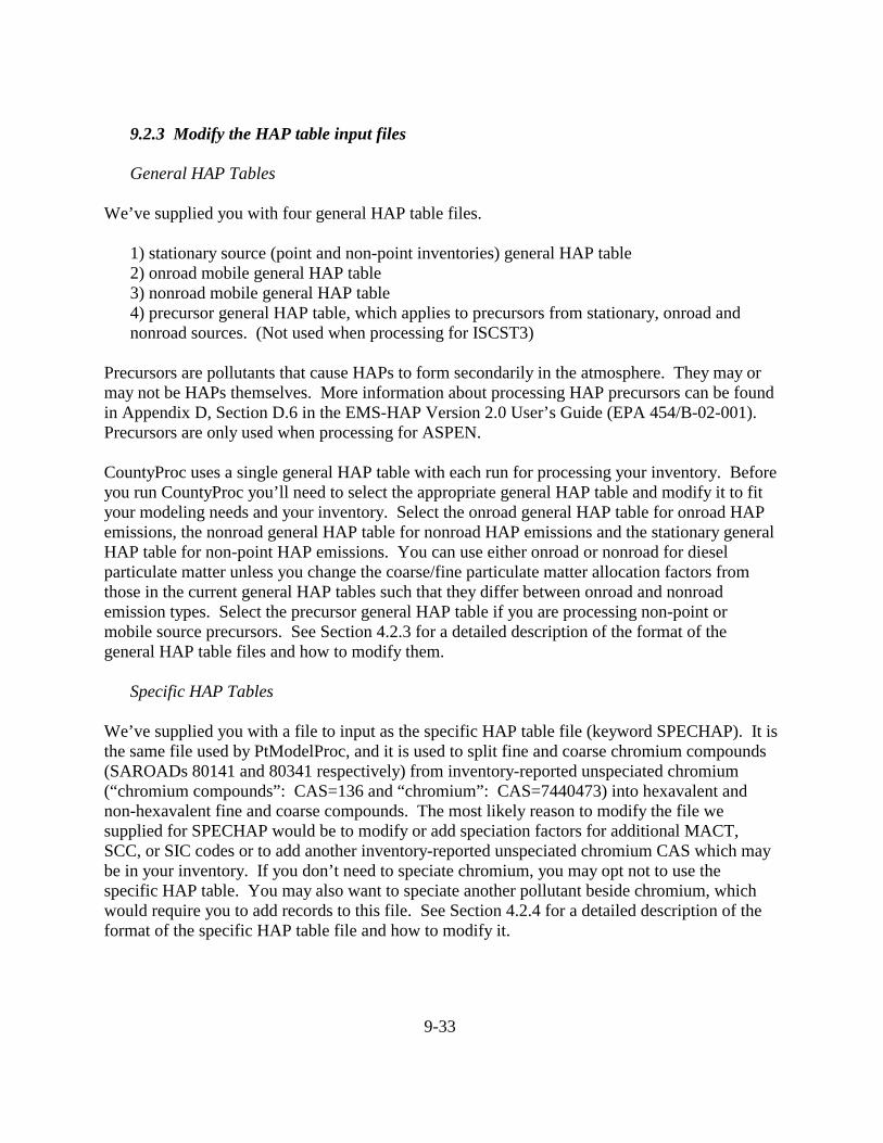
9-33
9.2.3 Modify the HAP table input files General HAP Tables We’ve supplied you with four general HAP table files.
1) stationary source (point and non-point inventories) general HAP table 2) onroad mobile general HAP table 3) nonroad mobile general HAP table
4) precursor general HAP table, which applies to precursors from stationary, onroad and nonroad sources. (Not used when processing for ISCST3)
Precursors are pollutants that cause HAPs to form secondarily in the atmosphere. They may or may not be HAPs themselves. More information about processing HAP precursors can be found in Appendix D, Section D.6 in the EMS-HAP Version 2.0 User’s Guide (EPA 454/B-02-001). Precursors are only used when processing for ASPEN. CountyProc uses a single general HAP table with each run for processing your inventory. Before you run CountyProc you’ll need to select the appropriate general HAP table and modify it to fit your modeling needs and your inventory. Select the onroad general HAP table for onroad HAP emissions, the nonroad general HAP table for nonroad HAP emissions and the stationary general HAP table for non-point HAP emissions. You can use either onroad or nonroad for diesel particulate matter unless you change the coarse/fine particulate matter allocation factors from those in the current general HAP tables such that they differ between onroad and nonroad emission types. Select the precursor general HAP table if you are processing non-point or mobile source precursors. See Section 4.2.3 for a detailed description of the format of the general HAP table files and how to modify them. Specific HAP Tables We’ve supplied you with a file to input as the specific HAP table file (keyword SPECHAP). It is the same file used by PtModelProc, and it is used to split fine and coarse chromium compounds (SAROADs 80141 and 80341 respectively) from inventory-reported unspeciated chromium (“chromium compounds”: CAS=136 and “chromium”: CAS=7440473) into hexavalent and non-hexavalent fine and coarse compounds. The most likely reason to modify the file we supplied for SPECHAP would be to modify or add speciation factors for additional MACT, SCC, or SIC codes or to add another inventory-reported unspeciated chromium CAS which may be in your inventory. If you don’t need to speciate chromium, you may opt not to use the specific HAP table. You may also want to speciate another pollutant beside chromium, which would require you to add records to this file. See Section 4.2.4 for a detailed description of the format of the specific HAP table file and how to modify it.

9-34
9.2.4 Modify the files that assign non-point and mobile source categories to source groups and source type (EMISBINS and CNTYUR)
You can modify the source group ancillary input file, EMISBINS, to specify different source groups for different non-point or mobile source categories or to incorporate differences in source group assignments due to the county urban/rural designation. For example, if you want to determine the contribution of onroad mobile sources in urban areas to your results, then assign a unique source group number (between zero and 9, inclusive, for ASPEN, or zero 00 and 99, inclusive, for ISCST3) in the EMISBINS to every onroad mobile source category in the urban column, and make sure that no other category (non-point, point, nonroad mobile, rural onroad mobile) uses this number. You must also make sure that the CNTYUR file correctly assigns each county to urban and rural classifications. If you are not assigning groups based on urban/rural classification, then you do not need to use the CNTYUR file. If the source categories in your inventory are different from those listed in the EMISBINS file, then you also need to assign values to the GROUP and CATCODE variables, and, an “A” or “M” for the source type (SRC_TYPE) variable if the source type is “area” or “major”, respectively (see footnote in 9.1.3 for definition). The EMISBINS file does not require a value for the source type variable; however, values of SRC_TYPE other than “A” or “M” will prevent any available MACT-based emission reductions from being applied. The format of EMISBINS is shown in Appendix A. The variable SCC (if processing 1999 NEI-based emissions) or CAT_NAME (if processing July 2001 version of the 1996 NTI) in this file is used to identify unique source categories. This file must contain one record for each category in the emission inventory. Note EMISBINS contains a unique category code (variable CATCODE) for each source category’s CATNAME variable (if processing July 2001 version of the 1996 NTI) for use in CountyProc’s growth and control module (see Section 9.2.7). The CATCODE variable is not used when processing 1999 NEI-based emissions. The last column in EMISBINS is the optional and aforementioned SRC_TYPE variable. The use of the category code makes the growth and control program run more efficiently. The CNTYUR contains a county-level urban/rural designation for every county in the contiguous United States. These designations were taken from those developed for the purposes of developing EPA's Integrated Urban Air Toxics Strategy9, based on the following: a county is considered "urban" if either 1) it includes a metropolitan statistical area with a population greater than 250,000; or 2) the U.S. Census Bureau designates more than fifty percent of the population as "urban." This information is used in conjunction with the group assignments for urban and rural sources from the EMISBINS file to assign source groups to each emission record. The CNTYUR file given in the batch file is similar to the CNTYUR files (a different file can be used for each projection scenario) used in when projecting emissions (see Table 9-11). The batch file CNTYUR file links inventory FIPS code to a county-level urban/rural designation for the purpose of allowing the user to group county-level sources in urban counties separately from

9-35
those in rural counties. The PROJECT file CNTYUR files assign a unique 5-character code to each county that the CountyProc projection algorithm can use to assign county-level emission reduction information (see Section 9.2.7) for user-specified county groups. If, in your emission projections, you choose to assign reduction information across urban and rural counties differently, then the CNTYUR file from the batch file will provide you the necessary information to distinguish between urban and rural counties.
9.2.5 Modify the source category-to- spatial surrogate cross-reference (SURRXREF) and optionally, the file that provides spatial surrogate descriptions (SURRDESC)
The most important option in spatial allocation is the selection of the appropriate spatial allocation surrogates. CountyProc assigns surrogates to mobile sources using the SURRXREF ancillary input file. This file cross-references each unique SCC code to a spatial surrogate code. This file also assigns surrogates for non-point sources (in conjunction with other spatial surrogate assignment files) in COPAX (see Section 2.2.3). You can modify the file to assign different surrogates to source categories or add new source categories (by SCC) to this file and assign surrogates to those. Appendix C provides a list of the currently available tract-level spatial surrogates (for EMS-HAP/ASPEN modeling or EMS-HAP/ISCST3 modeling using the tract approach) for non-point, onroad, and nonroad mobile inventories. CountyProc will use the optional comma-delimited file SURRDESC to provide list file outputs that include spatial surrogate descriptions. CountyProc will output a comma-delimited file called “FIPS_nonmatch_SCC_SURR.csv” containing those sources (FIPS/SCC combination) for which the assigned surrogate has no data in that particular county. The file will include county FIPS code, SCC, SCC description, assigned surrogate, and surrogate description for each FIPS/SCC combination. Each data record indicates a county-level emission source that was assigned a surrogate but for which surrogate data in the SAFFILE files do not exist. Note that this file is not produced when you are running the July 2001 version of the 1996 non-point inventory. CountyProc will re-assign these sources to the default surrogate (keyword DEFLTSAF) provided in the batch file (see Table 9-10 in section 9.2.8). 9.2.6 Modify the temporal allocation factor file (TAFFILE) The temporal allocation factor (TAF) file is a common file used for point, non-point and mobile sources. In this file, the temporal allocation factors are cross-referenced by 8-digit Source Classification Codes (SCC) or 10-digit Area and Mobile System (AMS) codes. The TAF file used when processing data for ASPEN allocates emissions for each source into average diurnal profiles that are representative of a typical day. The TAF file used when processing data for ISCST3 allocates emissions for each source into hourly emissions representing each of three day types in each of four seasons. You can change temporal allocation factors for source categories in these files and you can add profiles for additional source categories.

9-36
9.2.7 Modify the growth factors and emission reduction information files Similar to PtGrowCntl (Chapter 6) all growth and control input files for CountyProc are assigned via the comma-delimited PROJECT file. Each data record in the PROJECT file represents a unique projection scenario. For each projection scenario, the growth and control algorithm can use the following input files, depending on the type of projection scenario you want to apply:
• GFMACT: MACT-based growth factor file to grow from the base year to a projected year
• GFSIC: SIC-based growth factor file to grow from the base year to a projected year • GFSCC: SCC-based growth factor file to grow from the base year to a projected year • CNTYUR: cross-reference file from county FIP code to county reduction code • MACTGEN: general MACT emission reduction information file • SPECFILE: pollutant specific MACT emission reduction information file • USERFILE: user-defined emission reduction information file
The MACT-based, SIC-based, and SCC-based growth factor files are specific to the emission inventory base year, and the year of the projection inventory. They are used in both non-point source processing and point source processing (PtGrowCntl). Possible modification of these files is described in Section 6.2.3. The file formats of GFMACT, GFSIC, and GFSCC are provided in Appendix A. The general MACT reduction information file (MACTGEN) and the specific MACT reduction information file (SPECFILE) are used for both non-point source processing and point source processing (PtGrowCntl). They provide the reduction information needed to calculate the projected emissions for the specified projection year (see Section 6.1.3). Modification of these files is described in Section 6.2.4 and the formats are provided in Appendix A. The user-defined emission reduction information file (USERFILE) allows you to define emission reduction information by any combination of process and pollutant information, specified by the source category, MACT code, and/or NTI-HAP variable. In addition, you can define any of this information for specific counties or groups of counties of your own creation (e.g., urban versus rural counties, counties in a specific metropolitan statistical area, or all counties within a state). The format for the user-defined reduction information file is provided in Appendix A. Note when specifying reduction information at the county level, the county control codes used in USERFILE must match the codes in the CNTYUR file (the one in the PROJECT file not the batch file) which define the specific counties represented by those codes. In cases where an emission inventory record is affected by more than one record in USERFILE, a specific order of precedence is followed as presented in Table 9-3 in Section 9.1.7. In general, the more specific information will replace the more general information.

9-37
When processing the July 2001 version of the 1996 NTI, the file EMISBINS, which you supply to CountyProc via the batch file (as opposed to the PROJECT file), also plays a role in emission projections. The EMISBINS file (also discussed in 9.2.4) is used to cross-reference a category name from the USERFILE file, and from your inventory, to a category code. CountyProc uses the category code (rather than the category name) in the growth and control module to allow the module to run more efficiently. You need to make sure that the category names in the EMISBINS file exactly match the names in your emissions inventory and in the USERFILE file. 9.2.8 Prepare your batch file The batch file serves two purposes: (1) allows you to pass “keywords” such as file names and locations, program options, and run identifiers to the program, and (2) sets up the execute statement for the program. Sample batch files for CountyProc are shown in Figures B-14, B-15, and B-16 of Appendix B. The best way to prepare your batch file is to use one of the samples we provide and modify it to fit your needs. CountyProc and PtGrowCntl (Chapter 6) differ from all other EMS-HAP programs because, as discussed in 9.1.1 and 9.1.7 and shown in Tables 9-1 and 9-2, they utilize an ancillary cross-reference file (PROJECT), which specifies all projection scenario-specific ancillary files and program options.
Specify your keywords
For CountyProc, you need to specify keywords in the batch file and, if you are doing projections, also in the PROJECT file. The PROJECT file is a comma-delimited file that contains file names and program options that instruct CountyProc how to perform various projection scenarios; this is discussed in detail in 9.1.7 and specifically in Table 9-2. You specify the filename for keyword PROJECT in the batch file. Table 9-10 shows you all the batch file keywords, and how to specify them for CountyProc. Use them to locate and name all input and output files and supply run identification information. Further, you can run the program for a single HAP or state and get diagnostic information on a particular census tract when processing for ASPEN or a particular grid cell when processing for ISCST3. Edit the contents of the PROJECT file (see Tables 9-2 and 9-11) to set the number of projection scenarios and CountyProc functions performed in each scenario. The batch files used for running CountyProc for ASPEN or ISCST3 are very similar. CountyProc will ignore any batch file variable it does not need (e.g., if MODEL = ASPEN, XORIG, YORIG, CELLSIZE, and ISCOUT will be ignored if present in the batch file.)
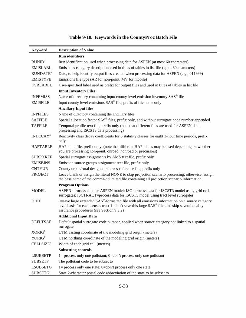
9-38
Table 9-10. Keywords in the CountyProc Batch File
Keyword Description of Value Run identifiers RUNIDa Run identification used when processing data for ASPEN (at most 60 characters) EMISLABL Emissions category description used in titles of tables in list file (up to 60 characters) RUNDATEa Date, to help identify output files created when processing data for ASPEN (e.g., 011999) EMISTYPE Emissions file type (AR for non-point, MV for mobile) USRLABEL User-specified label used as prefix for output files and used in titles of tables in list file Input Inventory Files INPEMISS Name of directory containing input county-level emission inventory SAS® file EMISFILE Input county-level emissions SAS® file, prefix of file name only Ancillary Input files INPFILES Name of directory containing the ancillary files SAFFILE Spatial allocation factor SAS® files, prefix only, and without surrogate code number appended TAFFILE Temporal profile text file, prefix only (note that different files are used for ASPEN data
processing and ISCST3 data processing) INDECAYa Reactivity class decay coefficients for 6 stability classes for eight 3-hour time periods, prefix
only HAPTABLE HAP table file, prefix only (note that different HAP tables may be used depending on whether
you are processing non-point, onroad, nonroad or precursors) SURRXREF Spatial surrogate assignments by AMS text file, prefix only EMISBINS Emission source groups assignment text file, prefix only CNTYUR County urban/rural designation cross-reference file, prefix only PROJECT Leave blank or assign the literal NONE to skip projection scenario processing; otherwise, assign
the base name of the comma-delimited file containing all projection scenario information Program Options MODEL ASPEN=process data for ASPEN model; ISC=process data for ISCST3 model using grid cell
surrogates; ISCTRACT=process data for ISCST3 model using tract level surrogates DIET 0=save large extended SAS®-formatted file with all emissions information on a source category
level basis for each census tract 1=don’t save this large SAS® file, and skip several quality assurance procedures (see Section 9.3.2)
Additional Input Data DEFLTSAF Default spatial surrogate code number, applied when source category not linked to a spatial
surrogate XORIGb UTM easting coordinate of the modeling grid origin (meters) YORIGb UTM northing coordinate of the modeling grid origin (meters) CELLSIZEb Width of each grid cell (meters) Subsetting controls LSUBSETP 1= process only one pollutant; 0=don’t process only one pollutant SUBSETP The pollutant code to be subset to LSUBSETG 1= process only one state; 0=don’t process only one state SUBSETG State 2-character postal code abbreviation of the state to be subset to

Table 9-10. Keywords in the CountyProc Batch File (continued)
9-39
Keyword Description of Value Diagnostics flags LDBG 1=printout of diagnostic information; 0=don’t ONECELL The selected single census tract (concatenation of FIPS code and tract identification code) or
grid cell (concatenation of column and row number) for which diagnostic information is printed Output files OUTFILES The output file directory ISCOUTc Output SAS® emissions file for data processed for ISCST3, prefix only WORK2 Directory for large temporary work files
a required only when processing data for ASPEN model; b required only when processing data for ISCST3 model using grid cell approach; c required only when processing data for ISCST3 model. Edit the contents of the PROJECT file to set the number of projection scenarios, functions performed in each scenario and names of the files containing the growth and reduction information. Table 9-11 provides the keywords in the PROJECT file, and Table 9-2 gives the file structure.
Table 9-11. PROJECT File Keywords for Selecting CountyProc Functions
Keyword Description of Value Ancillary files: (1) assign as ‘NONE’ or leave blank to prevent function, or (2) assign a file
name (provide prefix of file name only) containing data to be used GFMACT MACT-based growth factors text file for specific base and future year GFSIC SIC-based growth factors text file for specific base and future year GFSCC SCC-based growth factors text file for specific base and future year MACTGEN General MACT-based emission reduction information text file SPECFILE Specific MACT-based emission reduction information text file USERFILE User-defined emission reduction information text file CNTYUR State/County FIPS code to county control code cross-reference text file Projection Scenario Options/ Parameters GCFLAG 0=produce county-level projected emissions; 1=produce model-level projected emissions YEARTYPE CALENDAR = Project Emissions beginning January 1 in the projected year
FISCAL = Project Emissions beginning October 1 in the year prior to the projected year GROWYEAR Year to which emissions are to be projected PNAME Parameter string used to produce the base name of the projection scenario-specific output inventory
SAS® file name (see Table 9-12 in Section 9.3.3). You must include values for all keywords in your batch file. In the PROJECT file, you must provide either names, the word “NONE” or “” for the projection scenario filenames depending on whether or not you want to perform the particular growth/control function associated with that file. For example, if you do not wish to apply any growth factors for a projection scenario, you can either put “NONE,NONE,NONE” (or, “,,,”) as the second, third, and fourth entries

9-40
(representing file names for GFMACT, GFSIC, and GFSCC) for that scenario. Note, do not include the double quotes in the PROJECT file. Prepare the execute statement The last line in the batch file runs the CountyProc program. In the sample batch files provided in Figures B-14, B-15, and B-16 of Appendix B, you will see a line preceding the run line that creates a copy of the CountyProc code having a unique name. It is this version of the program that is then executed in the last line. If you do this, the log and list files created by this run can be identified by this unique name. If you don’t do this and run the program under a general name, every run of CountyProc will create a log and list file that will replace any existing files of the same name. You may find that you need to define a special area on your hard disk to use as workspace when running CountyProc. In the sample batch file, a directory for workspace is defined by the keyword WORK2. The directory you reference here must be created prior to running the program. 9.2.9 Execute CountyProc There are two ways to execute the batch file. One way is to type ‘source’ and then the batch file name. Alternatively, first set the permission on the file to ‘execute.’ You do this by using the UNIX chmod command and adding the execute permission to yourself, as the owner of the file, to anyone in your user group, and/or to anyone on the system. For example, ‘chmod u+x CountyProc.bat’ gives you permission to execute the batch file. Refer to your UNIX manual for setting other permissions. After you have set the file permission, you can execute the batch file by typing the file name on the command line, for example, ‘CountyProc.bat’. 9.3 How Do I Know My Run of CountyProc Was Successful? 9.3.1 Check your SAS® log file You should review the output log file to check for errors or other flags indicating incorrect processing. This review should include searching the log files for occurrences of the strings “ERROR”, “WARNING”, “not found”, and “uninitialized”. These can indicate problems with input files or other errors. The log file contains details on the number of records in the intermediate files created and modified during processing. You should check this information to make sure it’s reasonable. The number of records after conversion from inventory pollutant codes to SAROAD codes can change for three reasons: 1) some pollutants are dropped here, 2) some pollutants are split into two pollutants, and 3) after the pollutants have been assigned to SAROAD code groups, the emissions are summed to the SAROAD level. The number of records should increase after

9-41
spatial allocation. The number of records decreases when the emissions file is collapsed to the source group level. 9.3.2 Check your SAS® list file The list file can contain the following information depending on the program control options you specified, such as the DIET option (1=yes, which suppresses some quality assurance outputs to the list file) and whether you are projecting emissions to a future year:
• The first 20 records in the emissions inventory • Contents of input emissions file • Emissions totals and record counts, by pollutant, for the input emission inventory • Summary of Input Emission Rates by Pollutant • Summary of Input Emission Rates by State • List of pollutants retained in the general HAP table • Warning message if there are pollutants in emissions file not matched to HAP table.
Lists the pollutant codes in emissions inventory not matched. • Warning message if records with no reactivity code were encountered when merging
reactivity codes with emissions. Prints the first 10 records and a summary of emissions by pollutant.
• Pollutant sums by pollutant before and after collapsing to SAROAD codes, and if available, after the application of factor from the specific HAP table
• Warning message if there are counties in the emissions file which do not have a match in the county urban/rural codes file
• Warning message if there are emissions categories not matched to source groups. Lists the unmatched categories.
• Table of assignment of spatial surrogates to source categories • Surrogate-level summary of emissions • Warning message if records with no matching surrogate code were encountered when
merging spatial surrogate codes with emissions. These are assigned to a default surrogate you choose in the batch file (keyword DEFLTSAF). Lists the SCC or AMS codes that did not match to spatial surrogates. Prints the first few non-matched records. Prints summaries of non-matched emissions by pollutant and by source category.
• Summary of emissions by pollutant after spatial surrogate matching • Spatial surrogates frequency table • Warning message if records with no matching spatial factors were encountered when
matching spatial surrogates with emissions. Lists the first few records with no factors. Summarizes emissions without factors by pollutant, by county, by source category, and by surrogate.
• Summary of emission rates by pollutant after spatial allocation • Summary of temporal profiles used • Summary of emission rates by pollutant after temporal factor merge

9-42
• Warning message if records with no matching TAFs were encountered when merging temporal allocation factors with emissions. Lists the SCC or AMS codes that did not match to temporal factors. Prints the first few non-matched records. Prints summaries of non-matched emissions by pollutant and by source category.
• Summary of emission rates by pollutant after collapsing source categories to source groups
• Summary of temporally allocated emissions by pollutant • List of general MACT reduction information • For each projection scenario in the PROJECT file, a warning message if general MACT
reduction information not found in inventory • For each projection scenario in the PROJECT file, a list of specific MACT reduction
information • For each projection scenario in the PROJECT file, a warning message if specific MACT
reduction information not found in inventory • For each projection scenario in the PROJECT file, a list of user-defined reduction
information • For each projection scenario in the PROJECT file, a warning message if user-defined
reduction information not found in inventory • For each projection scenario in the PROJECT file, a summary of reduction information
applied to emissions • Run times for processing components • Pollutant sums by source category group • Emissions summaries by reactivity class • Output of Contents Procedure for the core SAS® output emission data set • Output of Contents Procedure for the extended SAS® output emission data set • Table of emissions totals by pollutant, with reactivity class, record counts, and the
average emissions for a tract • Summary of emissions by state • Frequencies of emissions sources by reactivity class • Emissions totals by reactivity class
At succeeding steps in the processing, emissions are summed and printed in the processing output files. You should review these after completion of program execution, looking for changes in emissions, which then would need to be explained. These are the processing points where emissions sums are reported:
• After reading the emissions, before any processing • Before collapsing from CAS pollutants to SAROAD pollutant groups • After collapsing from CAS pollutants to SAROAD pollutant groups after application of
both the general and specific HAP tables • After match/merge of spatial surrogates with emissions • After spatial allocation of emissions

9-43
• After temporal allocation of emissions (unless DIET = 1) • When writing out the ASPEN emissions files
You can inspect the diagnostics (in the list file) that CountyProc provides of the temporal allocation step (non-matched categories to temporal profiles) to see which emissions categories need to be added to the temporal allocation factor file, and the importance of each in terms of the amount of emissions in the categories. Similarly, you can inspect diagnostics of the spatial allocation process. If a source category is present in the emissions file but absent in the spatial surrogate file, the emission record cannot be matched and is assigned the default surrogate, population. In this case a warning message is printed to the CountyProc output file along with a summary of how many emission records were not matched, and a summary by source category of the non-matched emissions. Inspection of this information allows you to see which emissions categories need to be added to the spatial surrogate file, and the importance of each of these in terms of the amount of emissions in the categories. The spatial allocation factors are matched to emissions records according to spatial surrogates. If these do not match properly, CountyProc prints a warning message and summaries of the problem. The most common cause of non-matches is counties or census tracts/grid cells missing from one or more spatial allocation factor files. Emission records not matched to spatial surrogates are assigned the user-defined surrogate (keyword DEFLTSAF in the batch file). The general and specific HAP table files are matched to emission records according to the inventory pollutant code. If a pollutant is present in the emissions file but absent in the general HAP table, the emission record cannot be matched. In this case a warning message is printed to the CountyProc output file along with a summary of how many emission records were not matched, and a summary by pollutant of the non-matched emissions. Inspection of this information allows you to see which pollutants need to be added to the general HAP table. The emissions source group assignment file (EMISBINS) is matched to emission records according to source category and county urban/rural designation. If a source category is present in the emissions file but absent in the EMISBINS file, the emission record cannot be matched. In this case a warning message is printed to the CountyProc list file along with a summary of how many emission records were not matched, and a summary by source category of the non-matched emissions. Inspection of this information allows you to see which source categories need to be added to the source group file. The county urban/rural designation file (CNTYUR) in the CountyProc batch file (Table 9-10) is matched to emission records according to FIPS state and county codes. If a county is present in the emissions file but absent in the county data file, the emission record cannot be matched. In this case a warning message is printed to the CountyProc output file along with a summary of how many emission records were not matched, and a summary by county of the non-matched

9-44
emissions. Inspection of this information allows you to see which counties need to be added to this ancillary file. As each of the three emission reduction information files used to project emissions to a future year are read, the information is listed in the CountyProc output file. After the information is assigned to the emission records, any emission reduction information not assigned is listed in the output file. This allows you to see exactly what reduction information is being applied to the inventory. For each projection scenario, after the projected emissions are computed, a summary of the grown emissions (after application of the growth factor) and the projected emissions (after application of emission reduction controls) for selected time periods is listed in the CountyProc output file. Inspection of this information allows you to see precisely how the reduction information was assigned and then applied to the emissions. 9.3.3 Check other output files The output files produced by CountyProc are discussed in Sections 9.1.9 (ASPEN processing), 9.1.10 (ISCST3 processing) and 9.1.11 (county-level projections). The particular outputs you get in a single run depend on the options you select (see 9.1.1). These are summarized, along with the naming scheme for the outputs, in Table 9-12. Tables 9-13 through 9-18 provides file formats for many of these output files. If you are processing for ASPEN and have selected to produce the ASPEN input files, you should check that all nine files were created and that emission data are included only in those files representing reactivity classes for which you know your inventory has emission data. You may also want to check the header of the files for the decay rate information. You should also, when processing data for ASPEN, check for the existence of the column-formatted ASCII file -if you have selected DIET=0. Table 9-13 shows the format for the column-formatted ASCII file. Table 9-14 shows the format for the core SAS® file produced when processing for ASPEN; this file is not produced when county-level projections are performed (GCFLAG=0). Table 9-15 shows the format for the extended SAS® file produced when processing for ASPEN; this is output if DIET=0. If you are processing data for ISCST3, you should check for the existence of the output inventory SAS® file which is similar (in that MACT and SIC-level emissions are not retained) to the core SAS® file created when processing data for ASPEN (Table 9-14). Table 9-16 provides the format for the ISCST3 core SAS® file; this file is used as input into CountyFinal, the last non-point and mobile source processing program you run that will create a portion of the SO pathway section of the ISCST3 run stream. If you have chosen DIET=0, then you will also get the extended SAS® file; Table 9-17 shows the format. If, for any of the projection scenarios, you have chosen to create county-level inventory outputs (GCFLAG=0), you will only get a county-level SAS® output file with the variables shown in

9-45
Table 9-18; the choice of the keyword MODEL has no effect on the contents of county-level inventory outputs. Note the variable CNTLCODE. This variable contains information about what reduction information (general MACT, specific MACT, and/or user-defined) was assigned to the emission record and how the information was combined for the assignment of the primary and additional reduction efficiencies. Reviewing the CNTLCODE variable can help confirm how your reduction strategies were used to project the emissions.
Table 9-12. CountyProc Output File Names (located in the OUTFILES directory) Output File ASPEN File Name* ISCST3 File Name*
ASPEN input files: produced when GCFLAG=1
EMISTYPE + “.” + USRLABEL + PNAME + “.” + SUBSETG + “.D” + RUNDATE + “.r” + REACT + “.inp”
Not Produced for ISCST3
ASPEN ASCII file: produced if DIET=0 and GCFLAG=1
EMISTYPE + USRLABEL + PNAME + “.txt”
Not Produced for ISCST3
Core Inventory SAS® file for ASPEN: produced if GCFLAG=1
“c” + EMISTYPE + USRLABEL + PNAME
Output SAS® file for input to CountyFinal for ISCST3: produced if GCFLAG=1
EMISTYPE + USRLABEL + PNAME
Extended Inventory SAS®: produced if DIET=0 or any time GCFLAG=0
EMISTYPE + USRLABEL + PNAME “X” + EMISTYPE + USRLABEL + PNAME
* PNAME is missing if you are not running COUNTYPROC with emission projections

9-46
Table 9-13. Format of CountyProc ASCII Data File Created when Processing Data for ASPEN
(Values in order listed) Description (Units or values are in parentheses) Type*
5-digit FIPS code; state and county combined A5
Census tract centroid location longitude (negative decimal degrees) 10.5
Census tract centroid location latitude (decimal degrees) 10.5
ASPEN Source type (0=points, 3=pseudo-points) A1
Urban/rural dispersion flag (1 for urban, 2 for rural) 1.0
ASPEN Stack ID (same as State/County FIPS code) A5
constant = 999. 6.0
constant = 999. 6.0
constant = 999. 6.0
constant = 999. 6.0
Unique pollutant group code (SAROAD code) A5
ASPEN source group (integer between 0 and 9, inclusive) A2
Emissions rate (grams/second) for the first 3-hour time period** E10.
Emissions rate, (grams/second) time period 2 ** E10.
Emissions rate, (grams/second) time period 3 ** E10.
Emissions rate, (grams/second) time period 4 ** E10.
Emissions rate, (grams/second) time period 5 ** E10.
Emissions rate, (grams/second) time period 6 ** E10.
Emissions rate, (grams/second) time period 7 ** E10.
Emissions rate, (grams/second) time period 8 ** E10.
Tract ID A6
Vent/stack flag A1
Building wake effects flag A1
Baseline annual emissions rate (tons/year) E12.5
Baseline annual emissions rate (grams/second) E12.5 * Ax = character string of length x, x.y = numeric format with y places right of decimal, Ex. = exponential ** Temporally allocated emission values represent projected emissions when you choose to perform EMS-HAP’s emission projection capabilities

9-47
Table 9-14. Variables Contained in CountyProc Core SAS® Output File Created when Processing Data for ASPEN
Variable Name Description (Units or values are in parentheses) Type*
CELL State and county FIPS codes concatenated with the 6-digit tract ID A11
EMIS Baseline annual emissions rate (grams/second) N
EMIS_TPY Baseline annual emissions rate (tons/year) N
FIPS State/county FIPS code A5
GROUP ASPEN source group (integer between 0 and 9, inclusive) A2
IBLDG Building wake effects flag A1
IVENT Vent/stack flag A1
LAT Census tract centroid location latitude (decimal degrees) N
LON Census tract centroid location longitude (negative decimal degrees) N
NOSC Excluded stability classes A6
NOWD Excluded wind directions A6
NOWS Excluded wind speeds A6
REACT Reactivity class (integer between 1 and 9, inclusive) N
SAROAD Unique pollutant-group code A5
SRCETYPE Source type (0=points, 3=pseudo-points) A1
STACKID State/county FIPS code A5
TEMIS1 Emissions rate (grams/second) for the first 3-hour time period ** N
TEMIS2 Emissions rate, (grams/second) time period 2 ** N
TEMIS3 Emissions rate, (grams/second) time period 3 ** N
TEMIS4 Emissions rate, (grams/second) time period 4 ** N
TEMIS5 Emissions rate, (grams/second) time period 5 ** N
TEMIS6 Emissions rate, (grams/second) time period 6 ** N
TEMIS7 Emissions rate, (grams/second) time period 7 ** N
TEMIS8 Emissions rate, (grams/second) time period 8 ** N
TRACTR Tract ID A6
UFLAG Urban/rural dispersion flag (1=urban, 2=rural) A1
WBANID Meteorological station ID A5 * Ax = character string of length x, x.y = numeric format with y places right of decimal ** Temporally allocated emission values represent projected emissions when you choose to perform EMS-HAP’s emission projection capabilities

9-48
Table 9-15. Variables Contained in CountyProc Extended SAS® Output File when Processing Data For ASPEN
Variable Name Description (Units or values are in parentheses) Type*
ADDNEFF a Reduction (%) for new sources to be applied in addition to primary reductions N
ADDXEFF a Reduction (%) for existing sources to be applied in addition to primary reduction N
ADD_RATE a Percentage of emissions attributable to new sources for the purpose of applying additional reductions
N
CATCODE Source category code specified in the source group cross-reference file A4
CELL State and county FIPS codes concatenated with the 6-digit tract ID A11
CNTLCODE a Control code indicating the reductions applied to emissions A60
EMIS Baseline annual emissions rate (tons/year) N
GROUP Source group A2
EXISTEFF a Primary percent reduction for existing sources N
GF a Growth factor N
GFCODEa growth factor application method A7
LAT Census tract centroid location latitude (decimal degrees) N
LON Census tract centroid location longitude (negative decimal degrees) N
MACT MACT code A7
NEW_EFF a Primary percent reduction for new sources N
NEW_RATE a Percentage of emissions attributable to new sources for the purpose of applying primary reductions
N
NTI_HAP Code identifying HAP on the Clean Air Act HAP list A3
REACT Reactivity class N
REPLACE a User-defined reduction flag (R=replace MACT-based reductions with user-defined reductions; A=apply user-defined reductions in addition to the primary MACT-based reductions)
A1
SAROAD Unique pollutant-group code (SAROAD) A5
SCC For the July 2001 version of the 1996 non-point NTI: inventory AMS code; otherwise: source category code (SCC)
A10
SCC_INV For the July 2001 version of the 1996 non-point NTI: inventory SCC code; otherwise: does not exist
A10

Table 9-15. Variables Contained in CountyProc Extended SAS® Output File when Processing Data For ASPEN (continued)
9-49
Variable Name Description (Units or values are in parentheses) Type*
SIC Standard Industrial Classification (SIC) code A4
SRC_TYPE Emission source type A1
FIPS State/county FIPS code A5
SURR Spatial allocation surrogate code N
TF3HR1-TFHR8
Temporal allocation factor (dimensionless) for 3-hour time periods 1-8 N
TEMIS1-TEMIS8
Emissions rate (tons/year), 3-hour time periods 1-8; represents projected emissions when projections are performed
N
UFLAG Urban/rural dispersion flag (1=urban, 2=rural) A1
USE2SAF Equals “Y” if batch file default surrogate (keyword DEFLTSAF) was applied A1
* Ax = character string of length x, N = numeric a Variables included only when emission projections are done (see Section 9.1.7)
Table 9-16. Variables Contained in CountyProc Core SAS® Output File Created when Processing Data for ISCST3
Variable Name
Description (Units or values are in parentheses) Type*
CELL Grid cell approach: 3-character column concatenated with the 3-character row Tract approach: State and county FIPS codes concatenated with the 6-digit tract ID
A6 A11
EMIS Baseline annual emissions rate (tons/year) N
GROUP ASPEN source group (integer between 0 and 9, inclusive) A2
SAROAD Unique pollutant-group code A5
TEMIS1-TEMIS288**
Temporally allocated hourly emissions for the four seasons, three day types (weekday, Saturday, Sunday), and 24 hours (tons/hour), calculated in CountyProc (see Section 9.1.5)
N
UTMXa UTM easting coordinate (meters), computed in CountyProc (see Section 9.1.4) N
UTMYa UTM northing coordinate (meters), computed in CountyProc (see Section 9.1.4) N * Ax = character string of length x, x.y = numeric format with y places right of decimal ** Temporally allocated emission values represent projected emissions when you choose to perform EMS-HAP’s emission projection capabilities a For grid cell approach only

9-50
Table 9-17. Variables Contained in CountyProc Extended SAS® Output File when
Processing Data for ISCST3
Variable Name Description (Units or values are in parentheses) Type*
ADDNEFF a Reduction (%) for new sources to be applied in addition to primary reductions N
ADDXEFF a Reduction (%) for existing sources to be applied in addition to primary reduction N
ADD_RATE a Percentage of emissions attributable to new sources for the purpose of applying additional reductions
N
CATCODE Source category code specified in the source group cross-reference file A4
CELL Grid cell approach: 3-character column concatenated with the 3-character row Tract approach: State and county FIPS codes concatenated with the 6-digit tract ID
A6 A11
CNTLCODE a Control code indicating the reductions applied to emissions A60
EMIS Baseline annual emissions rate (tons/year) N
GROUP Source group A2
EXISTEFF a Primary percent reduction for existing sources N
GF a Growth factor N
GFCODE a Growth factor application method A7
MACT MACT code A7
NEW_EFF a Primary percent reduction for new sources N
NEW_RATE a Percentage of emissions attributable to new sources for the purpose of applying primary reductions
N
NTI_HAP Code identifying HAP on the Clean Air Act HAP list A3
REPLACE a User-defined reduction flag (R=replace MACT-based reductions with user-defined reductions; A=apply user-defined reductions in addition to the primary MACT-based reductions)
A1
SAROAD Unique pollutant-group code A5
SCC For the July 2001 version of the 1996 non-point NTI: inventory AMS code or AMS code assigned in COPAX; otherwise: source category code (SCC)
A10
SCC_INV For the July 2001 version of the 1996 non-point NTI: inventory SCC code; otherwise: does not exist
A10
SIC Standard Industrial Classification (SIC) code A4
SRC_TYPE Emission source type A1

Table 9-17. Variables Contained in CountyProc Extended SAS® Output File when Processing Data for ISCST3 (continued)
9-51
Variable Name Description (Units or values are in parentheses) Type*
TEMIS1-TEMIS288
Temporally allocated hourly emissions for the four seasons, three day types (weekday, Saturday, Sunday), and 24 hours (tons/hour), calculated in CountyProc (see Section 9.1.5); represents projected emissions when projections are performed
N
UTMXb UTM easting coordinate (meters), computed in CountyProc (see Section 9.1.4) (for grid cell approach only)
N
UTMYb UTM northing coordinate (meters), computed in CountyProc (see Section 9.1.4) (for grid cell approach only)
N
* Ax = character string of length x, N = numeric a Variables included only when emission projections are done (see Section 9.1.7) b For grid cell approach only
Table 9-18. Variables Contained in CountyProc Extended SAS® Output File when
Projecting County-Level Emissions (GCFLAG=0)
Variable Name Description (Units or values are in parentheses) Type*
ADDNEFF Reduction (%) for new sources to be applied in addition to primary reductions N
ADDXEFF Reduction (%) for existing sources to be applied in addition to primary reduction N
ADD_RATE Percentage of emissions attributable to new sources for the purpose of applying additional reductions
N
CATCODE Source category code specified in the source group cross-reference file A4
CAT_NAME For the July 2001 version of the 1996 non-point NTI: inventory category name; otherwise: does not exist
A90
CDATE Compliance date in SAS® format: number of days since January 1, 1960; used to determine how MACT-based emissions reductions are applied (Section 6.1.3)
N
CNTLCODE Control code indicating the reductions applied to emissions A60
CNTYCODE County code type used when applying user-defined reductions to specific counties (see Section 6.1.4); will be a 1-character variable with blank values if user-defined reductions are not applied
A5
EMIS Baseline annual emissions rate (tons/year) N
EMISGC Projected annual emissions rate (tons/year); calculated only for county-level projected emissions
N
EXISTEFF Primary percent reduction for existing sources N
FIPS State/county FIPS code A5
GF Growth factor N

Table 9-18. Variables Contained in CountyProc Extended SAS® Output File when Projecting County-Level Emissions (GCFLAG=0) (continued)
9-52
Variable Name Description (Units or values are in parentheses) Type*
GFCODE Growth factor application method A7
GROUP Source group A2
MACT MACT code A7
NEW_EFF Primary percent reduction for new sources N
NEW_RATE Percentage of emissions attributable to new sources for the purpose of applying primary reductions
N
NTI_HAP Code identifying HAP on the Clean Air Act HAP list A3
REPLACE User-defined reduction flag (R=replace MACT-based reductions with user-defined reductions; A=apply user-defined reductions in addition to the primary MACT-based reductions)
A1
SAROAD Unique pollutant-group code (SAROAD) A5
SCC For the July 2001 version of the 1996 non-point NTI: inventory AMS code; otherwise: source category code (SCC)
A10
SCC_INV For the July 2001 version of the 1996 non-point NTI: inventory SCC code; otherwise: does not exist
A10
SIC Standard Industrial Classification (SIC) code A4
SRC_TYPE Emission source type A1
* Ax = character string of length x, N = numeric

10-1
CHAPTER 10
County-level Non-point and Mobile Source Processing The Final Format Program (CountyFinal) for ISCST3
The flowchart below (Figure 10-1) shows how CountyFinal fits into EMS-HAP’s mobile and non-point source processing for the ISCST3 model. You don’t use this program if you are processing emissions for ASPEN. The non-point or mobile source inventory you input to CountyFinal is the output from CountyProc (Chapter 9). You use the output of CountyFinal to assist you in appending these sources to the SO pathway section of the ISCST3 run stream that was created by PtFinal_ISCST3.
Figure 10-1. Overview of CountyFinal within EMS-HAP for County-level Non-point and Mobile Source Processing
County-level onroad mobile source emissions file
Include files for the SO pathway section of the ISCST3 run stream for grid cell or tract-level non-point, or nonroad mobile sources
County-level non-point or nonroad source emissions file
CountyProc
To EMS-HAP Point
source programs,
starting with
PtDataProc (Chapter 3)
Allocated emissions
CountyFinal
Include files for the SO pathway section of the ISCST3 run stream for grid cell or tract-level onroad mobile sources
CountyFinal
COPAX
CountyProc
County-level emissions

10-2
10.1 What is the function of CountyFinal? The Final Format Program (CountyFinal) for ISCST3 prepares the grid cell or tract-level non-point or mobile source emissions from CountyProc for their treatment as ISCST3 area sources in the ISCST3 model. It also creates, for these sources, the include files for the SO pathway section of the ISCST3 run stream file and a text file containing source identification information for the source groups represented. You are responsible for adding both (1) the contents of this source identification information text file, and (2) statements to call the include files, to the existing SO pathway section of the ISCST3 run stream file created from PtFinal_ISCST3. The specific functions of CountyFinal are listed below. You control how the first three functions are performed in any given execution of CountyFinal (see Table 10-8 in Section 10.2.4 for details on how to do this). C CountyFinal assigns default release parameters to emission sources C CountyFinal assigns available pollutant-specific particle size data and gas deposition data C CountyFinal assigns available emission source elevation data by modeling grid cell or census
tract C CountyFinal converts each of the 288 temporally allocated emission rates and baseline
emissions to grams/sec-m2
C CountyFinal removes emission sources that are outside of modeling
C CountyFinal assigns source identification codes needed for the ISCST3 SO pathway section files
C CountyFinal calculates UTM coordinates for the tract-level approach and adjusts UTM
coordinates of emission sources for both approaches C CountyFinal creates include files for the SO pathway section of the ISCST3 run stream C CountyFinal creates text files containing source identification information for the source
groups for inclusion in the SO pathway section of the ISCST3 run stream Figure 10-2 shows a flowchart of CountyFinal. The following sections describe the above bullets.

10-3
Figure 10-2. CountyFinal Flowchart
Reads keywordsBatch file containing keywords e.g., file names and locations,
program options
Include files for SO pathway of ISCST3 run stream.Text file containing source groupings for inclusion in the SO pathway section of the ISCST3 run stream
CountyFinal: MACRO MERGASD Reads default gas deposition parameter file and assigns to emissions by pollutant
Default gas deposition parameter file (keyword DEFGAS)
Emission inventory file (keyword INSAS)
CountyFinal: MACRO MERGELEV Reads grid cell or tract elevation file and assigns elevation data to emissions by grid cell or tract.
CountyFinal: MACRO MERGPART Reads pollutant-level particle size distribution file and assigns to emissions by pollutant.
Pollutant-level particle size distribution file
(keyword DEFPART)
Grid cell elevation file (keyword ELEVDAT)
CountyFinal: MACRO SOPATH Assigns default release parameters to all sources in order to model as ISCST3 area sources. Removes emissions from grid cells outside of modeling domain. Adjusts UTM coordinates of emission sources for grid cell approach. Assigns source identification codes needed in the SO pathway of run stream. Creates text file to be used as part of the SO pathway of ISCST3 run stream. Writes include files for SO pathway of run stream.
CountyFinal: MACRO GETINFO Reads emissions inventory. Sums emissions for each source group, pollutant, and grid cell or tract. Converts emissions to units of grams/sec-m2.

10-4
10.1.1 CountyFinal assigns default release parameters to emission sources The ISCST3 model requires release parameter and source dimensional information for each source to be modeled. All (non-point and mobile) sources processed by CountyProc and CountyFinal are prepared for ISCST3 modeling as ISCST3 area sources; each grid cell or tract represents an ISCST3 area source. The release parameters and source dimensional information are shown in Table 10-1 for each approach. When processing using the grid cell approach, only REL_HGT and DELTA_X are required for ISCST3 processing. When processing using the tract-level approach, REL_HGT and NVERT are required. When processing using the grid cell approach, CountyFinal assigns most of the default release parameters to each grid cell based on the keywords you provide in the batch file (see Table 10-9, Section 10.2.4); the only exception is the variable ROTATE, which is hard-coded in CountyFinal as 0 (zero) degrees because the grid cells are square (DELTA_X = DELTA_Y) with no rotation. DELTA_X and DELTA_Y are based your grid cell dimensions. For example, if you are using a 1 by 1 km modeling domain grid, then you would set CELLSIZE=1000 meters, and DELTA_X and DELTA_Y would be 1000 meters. When using the tract-level approach, only REL_HGT is assigned from keywords from the batch file. NVERT is assigned in EMS-HAP; values of NVERT come from the tract vertices ancillary file (TRACTFILE).
Table 10-1. Default ISCST3 Area Source Release Parameters and Source Dimensions
Variable Name
Release Parameter Keyword Used to Assign Value
When using the grid cell based spatial allocation approach
REL_HGT release height (meters) ARELHGT
DELTA_X length of X side of source (meters) CELLSIZE
DELTA_Y length of Y side of source (meters) CELLSIZE
ROTATE orientation angle of rectangle for source (degrees from North) -------- *
SIGMA_Z initial vertical dimension of plume (meters) AINPLUM
When Using the Tract-level spatial allocation approach
REL_HGT release height (meters) ARELHGT
NVERT number of vertices for each census tract ------------
SIGMA_Z Initial vertical dimension of plume (meters) AINPLUM * A rotation angle of 0 (zero) is hard coded in CountyFinal
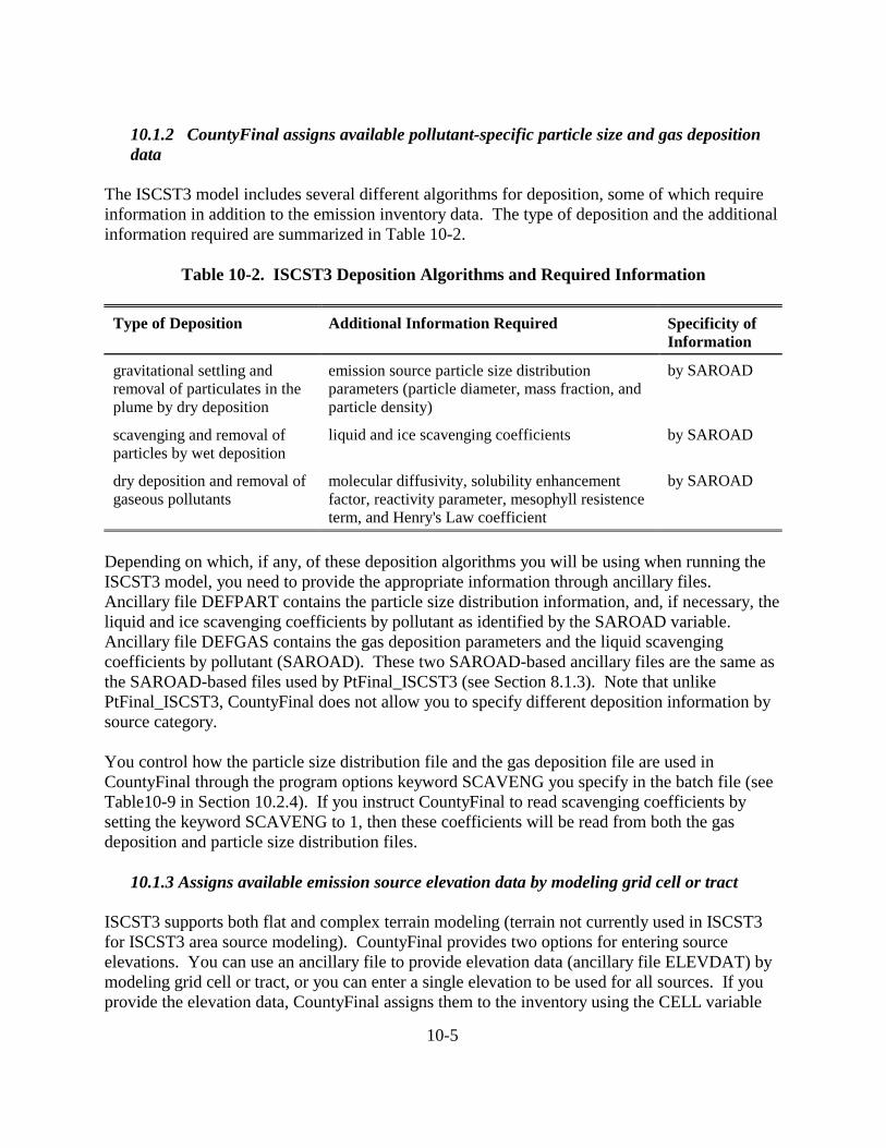
10-5
10.1.2 CountyFinal assigns available pollutant-specific particle size and gas deposition data
The ISCST3 model includes several different algorithms for deposition, some of which require information in addition to the emission inventory data. The type of deposition and the additional information required are summarized in Table 10-2.
Table 10-2. ISCST3 Deposition Algorithms and Required Information
Type of Deposition Additional Information Required Specificity of Information
gravitational settling and removal of particulates in the plume by dry deposition
emission source particle size distribution parameters (particle diameter, mass fraction, and particle density)
by SAROAD
scavenging and removal of particles by wet deposition
liquid and ice scavenging coefficients by SAROAD
dry deposition and removal of gaseous pollutants
molecular diffusivity, solubility enhancement factor, reactivity parameter, mesophyll resistence term, and Henry's Law coefficient
by SAROAD
Depending on which, if any, of these deposition algorithms you will be using when running the ISCST3 model, you need to provide the appropriate information through ancillary files. Ancillary file DEFPART contains the particle size distribution information, and, if necessary, the liquid and ice scavenging coefficients by pollutant as identified by the SAROAD variable. Ancillary file DEFGAS contains the gas deposition parameters and the liquid scavenging coefficients by pollutant (SAROAD). These two SAROAD-based ancillary files are the same as the SAROAD-based files used by PtFinal_ISCST3 (see Section 8.1.3). Note that unlike PtFinal_ISCST3, CountyFinal does not allow you to specify different deposition information by source category. You control how the particle size distribution file and the gas deposition file are used in CountyFinal through the program options keyword SCAVENG you specify in the batch file (see Table10-9 in Section 10.2.4). If you instruct CountyFinal to read scavenging coefficients by setting the keyword SCAVENG to 1, then these coefficients will be read from both the gas deposition and particle size distribution files. 10.1.3 Assigns available emission source elevation data by modeling grid cell or tract ISCST3 supports both flat and complex terrain modeling (terrain not currently used in ISCST3 for ISCST3 area source modeling). CountyFinal provides two options for entering source elevations. You can use an ancillary file to provide elevation data (ancillary file ELEVDAT) by modeling grid cell or tract, or you can enter a single elevation to be used for all sources. If you provide the elevation data, CountyFinal assigns them to the inventory using the CELL variable

10-6
assigned in CountyProc (see Section 9.1.4). If you want to use a single elevation for all sources, provide this value through the batch file keyword DEFELEV (see Table 10-9 in Section 10.2.4). More information on assigning source elevations can be found in Section 8.1.5, which discusses the assignment of elevations to point sources.
10.1.4 CountyFinal converts each of the 288 temporally allocated emission rates and baseline emissions to grams/sec-m2
CountyFinal converts the temporally allocated emissions (variables TEMIS1-TEMIS288) from tons/hour to grams/sec-m2 according to Equation 10-1, below. CountyFinal also converts the baseline emissions (EMIS) from tons/year to grams/sec-m2 according to Equation 10-2, below. The variable EMIS_TPY retains the baseline emissions in tons/year (Table 10-10). EQUATIONS USED WHEN MODELING GRID CELLS
Eg/s-m2(i) = Etons/hour(i) x [(1 hr/3600 sec) x (907,184grams/ton)] / (CELLSIZE)2 (eq. 10-1)
Eg/s-m2 = Etons/year x [(1 year/365 days) x (1 day/24 hrs)x(1 hr/3600 sec)x (907,184grams/ton)]/(CELLSIZE)2 (eq. 10-2)
where:
Eg/s-m2(i)= emissions in grams/second/meter2 for time block i (where i represents one of the 288 time blocks; e.g. time block i=1 represents the first hour of a winter weekday)
Eg/s-m2 = emissions in grams/second/meter2
Etons/hour(i) = emissions in tons/hour for time block i
Etons/year = emissions in tons/year
CELLSIZE = for grid cell approach: this is length of grid cell side, keyword CELLSIZE (see Table 10-9 in Section 10.2.4).
EQUATIONS USED WHEN MODELING CENSUS TRACTS
Eg/s-m2(i) = Etons/hour(i) x [(1 hr/3600 sec) x (907,184grams/ton)] / (CELLSIZE) (eq. 10-1)
Eg/s-m2 = Etons/year x [(1 year/365 days) x (1 day/24 hrs)x(1 hr/3600 sec)x (907,184grams/ton)]/(CELLSIZE) (eq. 10-2)
where:
Eg/s-m2(i)= emissions in grams/second/meter2 for time block i (where i represents one of the 288 time blocks; e.g. time block i=1 represents the first hour of a winter weekday)
Eg/s-m2 = emissions in grams/second/meter2
Etons/hour(i) = emissions in tons/hour for time block i
Etons/year = emissions in tons/year
CELLSIZE = for tract-level approach: the tract area in square meters, variable CELLSIZE is contained in the tract vertex ancillary file (TRACTFILE). Therefore in eq. 10-1 and eq. 10-2, for the tract-level approach, CELLSIZE is not squared.

10-7
10.1.5 CountyFinal removes emission sources that are outside of modeling domain When using the grid cell approach, CountyFinal windows the inventory to exclude any grid cells that are outside of the modeling domain. The CELL variable, created during spatial allocation for ISCST3 in CountyProc (see Section 9.1.4), contains the column and row from each grid cell. The first row and column delineate the southern and western extent of the domain. Grid cells are outside the domain if they have a column or row greater than the maximum column and row for the domain, or, if they are less than 1. You provide the modeling domain information through the keywords MAXCOL and MAXROW in the batch file (see Table 10-9 in Section 10.2.4). When using the tract-level approach, CountyFinal will subset the domain by dropping any tract-level emissions that are not associated with tracts in the TRACTFILE you supply (see 10.2.3).
10.1.6 CountyFinal assigns source identification codes needed for the ISCST3 SO pathway section files
CountyFinal assigns a source identification code to each emission record for use in the ISCST3 model. This identification code is created from the source group (variable GROUP, see Section 9.1.5), the RUN_ID keyword provided in the batch file (see Table 10-9 in Section 10.2.4), and a sequential number. CountyFinal determines this number by arranging the inventory by pollutant and source group (variables SAROAD and GROUP) and numbering the emission records sequentially within each source group (remember that separate run stream and include files are created for each pollutant). The one character RUN_ID is included in the source identification code to allow the ISCST3 model to distinguish between emission sources from different runs of EMS-HAP with different inventories that may have the same source group (e.g., the non-point source inventory and the point source inventory). When running ISCST3, the “include” files containing the emission data from these separate runs are combined. Thus, without the RUN_ID, the same source identification code could be given to sources from different runs of EMS-HAP for different inventories. To avoid this, specify a different value for RUN_ID for each different EMS-HAP run that you plan to use within the same ISCST3 run. RUN_ID is also used by PtFinal_ISCST3 (see 8.1.6) in the same way, so you need to make sure to use different values for RUN_ID when running this program as well. For example, if you have two PtFinal_ISCST3 runs, you can choose “A” for the first run and “B” for the second. You can then choose “C” when running CountyFinal for non-point sources and “D” when running for nonroad sources.
10.1.7 CountyFinal calculates UTM coordinates for the tract-level approach and adjusts UTM coordinates of emission sources for both approaches
Within the ISCST3 model, only six significant digits are used for the UTM coordinates of any source; it is possible that some sources have the UTM coordinates greater than 1,000,000 meters. To avoid the truncation of such coordinates in the ISCST3 model, CountyFinal adjusts all of the coordinates relative to the origin (southwest corner) of the modeling domain for the grid cell approach. The keywords X_ORIG and Y_ORIG, provided in the batch file (see Table 10-9 in

10-8
Section 10.2.4), are used in the following equations to perform this adjustment.
Adjusted UTMX = UTMX - X_ORIG (Eq. 10-3)
Adjusted UTMY = UTMY - Y_ORIG (Eq. 10-4)
Where:
UTMX = UTM easting coordinate (meters)
X_ORIG = UTM easting coordinate of grid origin
UTMY = UTM northing coordinate (meters)
Y_ORIG = UTM northing coordinate of grid origin
For the tract-level approach, the tract vertices’ coordinates are in degrees latitude and longitude. CountyFinal will calculate UTM coordinates based on the UTM zone assigned by the keyword REF_ZONE in the CountyFinal batch file. The UTM coordinates are then adjusted relative to the southwest corner of domain, similar to Eq. 10-3 and Eq. 10-4. If any tracts in the TRACTFILE have vertices that are south or west of the southwest corner of the domain that you specify in the batch file (X_ORIG and Y_ORIG), these vertices will have negative UTMX and or UTMY coordinates. To avoid this, you can modify the TRACTFILE to remove any such tracts. However, no computational problems will occur if negative coordinates are assigned.
10.1.8 CountyFinal creates include files for the SO pathway section of the ISCST3 run stream
In order to reduce the size of the SO pathway section of the run stream text files, CountyFinal uses the “include file” feature of ISCST3 run streams. The ISCST3 model processes only one pollutant during a run; therefore, CountyFinal creates separate include files for each pollutant, as identified by the pollutant SAROAD code. Table 10-3 shows a list of the include files and when they are created, and Table 10-4 shows how CountyFinal names them. After CountyFinal is complete, for each pollutant (SAROAD), you need to reference these include files in an existing SO pathway section of a run stream text file (use the one created by PtFinal_ISCST3).

10-9
Table 10-3. ISCST3 SO Pathway Run Stream Include Files
Include File Contents When File is Created
hourly emission factors
288 temporally allocated emission rates (inventory variables TEMIS1-TEMIS288)
For each SAROAD in inventory
emission source data
each file contains source location coordinates, stack parameters for point sources, release parameters for area and volume sources, and emission rates [set to 1] for each source
For each SAROAD in inventory
particle size distribution data/scavenging coefficients
particle diameter, mass fraction, and particle density and, if provided, liquid and ice scavenging coefficients (see Section 10.1.4)
Only if particle size distribution data is provided (ancillary file DEFPART is not equal to “NONE” or left blank), and pollutant is in the particle size distribution file
gas deposition parameters
molecular diffusivity, solubility enhancement factor, reactivity parameter, mesophyll resistence term, and Henry's Law coefficient (see Section 10.1.4)
Only if gas deposition data is provided (ancillary file DEFGAS is not equal to “NONE” or left blank), and pollutant is in the gas deposition file
Table 10-4. ISCST3 Include File Names
Type of Include File File Name (located in OUTFILES directory)Hourly emission factors “hrlyemis_” + RUN_ID + “.” + SAROAD
Emission source data “grid” + EMISBIN + RUN_ID + “.” + SAROAD
Particle size distribution data/scavenging coefficients
“particle_” + RUN_ID + “.” + SAROAD
Gas deposition parameters “gasdepo_” + RUN_ID + “.” + SAROAD

10-10
10.1.9 CountyFinal creates text files containing source identification information for the source groups for inclusion in the SO pathway section of the ISCST3 run stream
The SO pathway section of the ISCST3 run stream file must contain source group information for every source in the include files. Therefore, in addition to the include files discussed above, CountyFinal creates, for each pollutant (SAROAD), a text file containing the range of source identification codes (see Section 10.1.7) for each source group in the include files. Table 10-5 provides the naming convention for these files. For each pollutant modeled with ISCST3, you must add, to an existing SO pathway section of the ISCST3 runstream file, the contents of the source grouping files as well as the references to the include files created by CountyFinal. An SO pathway section will exist if the pollutant had sources that made it through PtFinal_ISCST3, that is, if any of the sources in the point source inventory had nonzero emissions in the modeling domain.
Table 10-5. Text File Names Containing Emission Source Groupings
Description File Name (located in OUTFILES directory)
Source groupings; one record per source group (GROUP), one file per pollutant (SAROAD)
“AMcats_” + RUN_ID + “.” + SAROAD
10.2 How do I run CountyFinal? 10.2.1 Prepare your inventory for input into CountyFinal The grid cell or tract-level non-point or mobile source inventory you use for input into CountyFinal is the output from CountyProc (see Chapter 9). This inventory will contain the necessary variables for CountyFinal, as shown in Table 10-6.

10-11
Table 10-6. Variables in the CountyFinal Input Inventory SAS® File
Variable Name
Data Description (Required units or values are in parentheses)
Type*
ADDNEFFa reduction (%) for new sources to be applied in addition to primary reductions; assigned in CountyProc (see Section 9.1.7)
N
ADDXEFFa reduction (%) for existing sources to be applied in addition to primary reductions; assigned in CountyProc (see Section 9.1.7)
N
ADD_RATEa percentage of emissions attributable to new sources for the purpose of applying additional reductions; assigned in CountyProc (see Section 9.1.7)
N
CATCODE Source category code specified in the source group cross-reference file A4
CELL Grid cell approach: 3-character column concatenated with the 3-character row Tract approach: State and county FIPS codes concatenated with the 6-digit tract ID
A6 A11
CNTLCODEa control code indicating the reductions applied to emissions; assigned in CountyProc (see Section 9.1.7)
A60
EMIS Baseline pollutant emissions value (tons/year) N
EXISTEFFa primary percent reduction for existing sources; assigned in CountyProc (see Section 9.1.7) N
FIPS 5-digit FIPS code (state and county combined) A5
GFa growth factor; assigned in CountyProc (see Section 9.1.7) N
GFCODEa growth factor application method; assigned in CountyProc (see Section 9.1.7) A7
GROUP Source group, assigned in CountyProc (see Section 9.1.3) A2
MACT MACT code A7
NEW_EFFa primary percent reduction for new sources; assigned in CountyProc (see Section 9.17) N
NEW_RATEa percentage of emissions attributable to new sources for the purpose of applying primary reductions; assigned in CountyProc (see Section 9.1.7)
N
NTI_HAP code identifying HAP on the Clean Air Act HAP list, assigned in CountyProc (see section 9.1.2) A3
REPLACEa user-defined reduction flag (R=replace MACT-based reductions with user-defined reductions; A=apply user-defined reductions in addition to the primary MACT-based reductions); assigned in CountyProc (see Section 9.1.7)
A1
SAROAD unique pollutant-group code, assigned in CountyProc (see Section 9.1.2) A5
SIC SIC code A4
SRC_TYPE code identifying source type, assigned in CountyProc (see Section 9.1.3) to apply reduction information by source type, it must have the value of ‘major’ or ‘area’ if you want to apply reduction information
A1
TEMIS1-TEMIS288
temporally allocated hourly emissions for the four seasons, three day types (weekday, Saturday, Sunday), and 24 hours (tons/hour), calculated in CountyProc (see Section 9.1.5)
N
UTMXb UTM easting coordinate (meters), computed in CountyProc (see Section 9.1.4) N
UTMYb UTM northing coordinate (meters), computed in CountyProc (see Section 9.1.4) N * Ax = character string of length x, I = integer, N = numeric a variables present only if you selected to project your emissions to a future year when you ran CountyProc b variables present only if you selected MODEL as ISC in CountyProc

10-12
10.2.2 Determine whether you need to modify the ancillary input files for CountyFinal An ancillary file is any data file you input to the program other than your emission inventory. Table 10-7 lists the ancillary input files for CountyFinal and when you may need to modify them. All ancillary files used by CountyFinal are optional; leaving the keywords in Table 10-9 blank, or assigning them values of “NONE” are the most efficient ways to prevent CountyFinal from using the functions associated with them.
Table 10-7. Ancillary Input File Keywords for CountyFinal
File Keyword
Purpose Need to Modify Files Supplied with EMS-HAP?
Format
DEFPART Provides the default particle size distribution data by pollutant
If you want to add new pollutants or replace parameter values with new values
Text
DEFGAS Provides the default gas deposition parameters by pollutant
If you want to add new pollutants or replace parameter values with new values
Text
ELEVDAT Provides terrain elevations (in meters) by modeling domain grid cell or tract
If you want to use elevation data for your domain and grid. Develop it if you use the grid cell approach. Modify it to include the tracts in your domain if you use the tract approach.
Text
TRACTFILE Used only when you use the tract-level approach: Provides vertices for each census tract in domain
Modify TRACTFILE to assure it includes the tracts associated with all counties, either partially or fully, in your modeling domain.
SAS®
10.2.3. Develop the particle size distribution, gas deposition, terrain elevation, and tract vertices files (DEFPART, DEFGAS, ELEVDAT, and TRACTFILE)
The DEFPART ancillary file contains information about particle size distributions that are applied to specific pollutants identified by the SAROAD variable. You can include up to 10 particle size classes. You must specify the number of size classes in the file. You can also include liquid and ice scavenging coefficients for each size class, but this is optional. The DEFGAS ancillary file contains gas deposition parameters that are assigned to the inventory by the SAROAD variable. The ELEVDAT ancillary file contains terrain elevation data by grid cell or census tract. We don’t supply elevation files as part of EMS-HAP for the grid cell approach since these are domain specific. Elevation data are available from the USGS Digital Elevation Model (DEM), at edcwww.cr.usgs.gov/doc/edchome/ndcdb/ndcdb.html. You need to grid this data to match your

10-13
grid specifications and domain. If you use the census tract approach, you should modify the file provided with EMS-HAP to assure that it includes the census tracts in your modeling domain. The TRACTFILE ancillary file, used only for the tract-level approach, contains the latitudes and longitudes for each census tract vertex for your domain. Each of the 48 conterminous states has its own separate ancillary SAS® file. If your domain covers more than one state, you will need to concatenate the files for the states in your domain before running CountyFinal. You provide the concatenated dataset as the TRACTFILE for CountyFinal. You may also want to remove tracts that are outside your modeling domain except for tracts that are included in a county that is only partially in your domain. That is, we recommend you do not split out tracts within the same county in TRACTFILE. 10.2.4 Prepare your batch file The batch file serves two purposes: (1) allows you to pass “keywords” such as file names and locations, program options and run identifiers to the program, and (2) sets up the execute statement for the program. Sample batch file for CountyFinal is shown in Figures B-17 and B-18 of Appendix B. The best way to prepare your batch file is to use one of the samples we provide and modify it to fit your needs. Specify your keywords Table 10-8 shows you how to specify keywords to select CountyFinal functions.
Table 10-8. Keywords for Selecting CountyFinal Functions CountyFinal Functions Keyword (values provided cause function to
be performed) Run model for
Grid cell based emissions MODEL=ISC
Tract-level based emissions MODEL=ISCTRACT
Use particle size distribution data provided
by pollutant without scavenging data DEFPART = Prefix of data file; SCAVENG = 0
by pollutant with scavenging data DEFPART = Prefix of data file; SCAVENG = 1
Use gas deposition parameters provided
without scavenging data DEFGAS = Prefix of data file; SCAVENG = 0
with scavenging data DEFGAS = Prefix of data file; SCAVENG = 1
Use elevation data provided ELEVDAT = Prefix of data file
Note that the keyword SCAVENG applies to both gaseous and particulate pollutants; thus, you

10-14
don’t have the option to use scavenging data for one of these pollutants types without the other. Table 10-9 describes all of the keywords required in the batch file. In addition to supplying all input and output file names and directories and program options, you must also supply additional input data (see “Additional Input Data” section in Table 10-9).
Table 10-9. Keywords in the CountyFinal Batch File Keyword Description of Value Input Inventory Files IN_DATA Input SAS® file directory INSAS Input inventory SAS® file name, prefix of file name only Ancillary Files (Prefix of file name provided with EMS-HAP in parentheses) REFFILES Ancillary file directory DEFPART Default pollutant-level particle distribution text file, prefix only (defpart);
leave blank or put “NONE” if no file is to be used DEFGAS Default pollutant-level gas deposition data text file, prefix only (defgas)
leave blank or put ‘NONE’ if no file is to be used ELEVDAT Gridded or tract-level terrain elevation data text file, prefix only;
leave blank or put “NONE” if no file is to be used (hstn-elev) TRACTFILEa Tract vertex SAS® file name, prefix of file name only. Program Options MODEL ISC=process grid cell data for ISCST3 model; ISCTRACT=process tract-level data for
ISCST3 model RUN_ID Run identification code used to insure unique ISCST3 source ID’s; typically used to
distinguish between point, non-point, and mobile inventory runs (one character limit) SCAVENG 1 = scavenging coefficients are included in the DEFPART or DEFGAS files;
0 = scavenging coefficients are not included in the DEFPART or DEFGAS files Additional Input Data DEFELEV Default elevation value used for all sources (meters); only used if ELEVDAT file prefix is
‘NONE’ or left blank X_ORIG UTM easting coordinate of the modeling grid origin (meters) Y_ORIG UTM northing coordinate of the modeling grid origin (meters) CELLSIZEb Width of each grid cell (meters) MAXCOLb Total number of columns in the modeling grid MAXROWb Total number of rows in the modeling grid ARELHGT Release height above ground (meters) AINPLUM Initial vertical dimension of plume (meters) REF_ZONEa UTM zone for ISCST3 model domain Output files OUTDATA Output SAS® file directory OUTSAS Output inventory SAS® file name, prefix only OUTFILES Output directory of SO pathway include files

10-15
aused for ISCTRACT only, leave blank or set to ‘NONE’ for ISC; bused for ISC only, leave blank or set to ‘NONE’ for ISCTRACT. You must include all batch file keywords in your batch file, even if they are related to a function that you don’t plan to perform. For example, if you set the ancillary file keyword DEFPART to “NONE" or leave blank, you still need keyword SCAVENG in your batch file; however, the value of this keyword may be blank. The program will not use the value provided in this circumstance; it is merely a placeholder value for the keyword. Prepare the execute statement The last line in the batch file runs the CountyFinal program. In the sample batch files provided in Figures B-17 and B-18 of Appendix B, you will see a line preceding the run line that creates a copy of the CountyFinal code with a unique name. It is this version of the program that is then executed in the last line. If you do this, the log and list files created by this run can be identified by this unique name. If you don’t do this and run the program under a general name, every run of CountyFinal will create a log and list file that will replace any existing files of the same name. You may find that you need to assign a special area on your hard disk to use as workspace when running CountyFinal. In the sample batch file, a work directory is defined on the last line following the execution of CountyFinal. For example, the command ‘sas CountyFinal_062000.sas -work /data/work15/dyl/’ assigns a SAS® work directory in the “/data/work1/dyl” directory. The directory you reference must be created prior to running the program. 10.2.5 Execute CountyFinal There are two ways to execute the batch file. One way is to type ‘source’ and then the batch file name. Alternatively, first set the permission on the file to ‘execute.’ You do this by using the UNIX chmod command and adding the execute permission to yourself, as the owner of the file, to anyone in your user group, and/or to anyone on the system. For example, ‘chmod u+x CountyFinal.bat’ gives you permission to execute the batch file. Refer to your UNIX manual for setting other permissions. After you have set the file permission, you can execute the batch file by typing the file name on the command line, for example, ‘CountyFinal.bat’. 10.3 How Do I Know My Run of CountyFinal Was Successful? 10.3.1 Check your SAS® log file You need to review the output log file to check for errors or other flags indicating incorrect processing. This review should include searching the log files for occurrences of the strings “ERROR”, “WARNING”, “not found”, and “uninitialized”. These can indicate problems with input files or other errors.

10-16
10.3.2 Check your SAS® list file This program only creates a list file when running CountyFinal with tract-level emissions (MODEL keyword = ISCTRACT). The list file lists the maximum number of census tract vertices in the domain. This number is important in that ISCST3 has a default maximum number of 20 vertices for an area source when processing area sources using the vertices’ coordinates. This number must be changed in the ISCST3 (NVMAX and NVMAX2 parameters in MODULES.FOR of ISCST3) model if the maximum number of vertices in your domain exceeds 20. For more details see the ISCST3 User’s Guide2. 10.3.3 Check other output files from CountyFinal To ensure that CountyFinal created all necessary include files, as well as the text files containing the source group information for each pollutant, you need to check the output file directory that you specified in the batch file using keyword OUTFILES. For each pollutant, in the gridded or tract-level mobile or non-point source inventory, CountyFinal always creates an emission factors include file, an emission source data file, and a text file listing source identification code ranges for the source groups. The creation of other include files containing particle size distribution data and gas deposition parameters depends on how you set the keywords in your batch file. In addition to the include files and text file of source groupings, CountyFinal creates an output SAS® inventory file, named by keyword OUTSAS. This file contains the variables listed in Table 10-10; some of these variables are only included depending on how you set the keywords in the batch file (see Table 10-9, Section 10.2.4). Note that since the emission data from the input SAS® inventory file are summed over the source group, pollutant, and grid cell or tract, specific source category information (SCC, SIC, MACT) is not included in this output file. Also note that the units of the temporally allocated emissions values are converted from tons/hour (input file) to grams/sec-m2, and the units of the baseline emission (EMIS) variable have been converted from tons/year to grams/sec-m2. The original baseline emissions value in tons/year is retained in the EMIS_TPY variable. Furthermore, note that the UTMX and UTMY (for gridded emissions only) variables are the pre-adjusted values and are thus the same as those in the inventory input to CountyFinal.

10-17
Table 10-10. Variables in the CountyFinal Output SAS® File Variable Name Data Description Type*ALPHAc Gas deposition parameter: solubility enhancement factor N
CELL Grid cell approach: 3-character column concatenated with the 3-character row Tract approach: State and county FIPS codes concatenated with the 6-digit tract ID
A6 A11
DIFFc Gas deposition parameter: molecular diffusivity (cm2/sec) N
EMIS Baseline pollutant emissions in grams/sec/m2 N
EMIS_TPY Annual grid cell baseline emission in tons/year N
GROUP Source group, assigned in CountyProc A5
HENRYc Gas deposition parameter: Henry’s Law coefficient N
LIQSCAVc Gas deposition parameter: liquid scavenging coefficient (1/(sec-mm/hr)) N
NUMCAT Number of particle size classes N
PDEN1-PDEN10a
Particle size distribution parameter: density (grams/cm3) N
PDIA1-PDIA10a Particle size distribution parameter: diameter (microns) N
PFRA1-PFRA10a Particle size distribution parameter: mass fraction N
PICE1-PICE10b Particle size distribution parameter: ice scavenging coefficient (1/(sec-mm/hr)) N
PLIQ1-PLIQ10b Particle size distribution parameter: liquid scavenging coefficient (1/(sec-mm/hr)) N
RSUBMc Gas deposition parameter: mesophyll resistence term (sec/cm) N
RXc Gas deposition parameter: reactivity parameter N
SAROAD unique pollutant-group code, assigned in CountyProc A5
SELEV Source elevation (m) N
SRCID Source identification code (see Section 10.1.6) A8
TEMIS1-TEMIS288 d
Temporally allocated hourly emissions for the four seasons, three day types (weekday, Saturday, Sunday), and 24 hours (tons/hour), calculated in CountyProc
N
UTMXe UTM easting coordinate (meters), computed in CountyProc N
UTMYe UTM northing coordinate (meters), computed in CountyProc N * Ax = character string of length x, N = numeric a variables added only when particle size distribution data are provided b variables added only when liquid/ice scavenging data are provided c variables added only when gas deposition parameters are provided d Temporally allocated emission values represent projected emissions when you choose to perform EMS-HAP’s emission projection capabilities e for grid cell based emissions (MODEL=ISC) only

10-18
This page intentionally blank

REFERENCES
1. User’s Guide: Assessment System for Population Exposure Nationwide (ASPEN, Version 1.1) Model. EPA-454-R-00-017, U.S. Environmental Protection Agency, Research Triangle Park, NC. March 2000.
2. User's Guide for the Industrial Source Complex (ISC3) Dispersion Models:
Volume I - User Instructions. EPA-454-/B-95-003a, U.S. Environmental Protection Agency, Research Triangle Park, NC. 1995b. http://www.epa.gov/scram001/userg/regmod/isc3v1.pdf
3. U.S. Environmental Protection Agency. Technology Transfer Network National
Air Toxics Assessment. The National-scale Air Toxics Assessment. http://www.epa.gov/ttn/atw/nata/ (Accessed July 2002).
4. Example Application of Modeling Toxic Air Pollutants in Urban Areas. EPA-
454-/R-02-003, U.S. Environmental Protection Agency, Research Triangle Park, NC. June 2002.
5. Driver, L.; Pope, A.; Billings, R.; Wilson, D. “The 1996 National Toxics
Inventory and Its Role in Evaluating the EPA’s Progress in Reducing Hazardous Air Pollutants in Ambient Air”, Presented at the 92nd Annual Meeting of the Air & Waste Management Association, St. Louis, MO, June 1999; paper 91-501.
6. Rosenbaum, A.S.; Ligocki, M.P.; Wei, Y.H. “Modeling Cumulative Outdoor
Concentrations of Hazardous Air Pollutants, Volume 1: text”; SYSAPP-99-96-33r2, Prepared for the U.S. Environmental Protection Agency, Office of Policy, Planning, and Evaluation, by Systems Applications International, Inc., San Rafael, CA. 1998, pp. 5-3 to 5-4.
7. Rosenbaum, A.S.; Ligocki, M.P.; Wei, Y.H. “Modeling Comulative Outdoor
Concentrations of Hazardous Air Pollutants, Volume 1: text”; SYSAPP-99-96-33r2, Prepared for the U.S. Environmental Protection Agency, Office of Policy, Planning, and Evaluation, by Systems Applications International, Inc., San Rafael, CA. 1998, pp. 5-9 to 5-11.
8. U.S. Environmental Protection Agency. Economic Growth Analysis System
Version 4.0 and Documentation, from the Technology Transfer Network Clearinghouse for Inventories and Emission Factors. http://www.epa.gov/ttn/chief/emch/projection/egas40/index.html (Accessed May, 2001)
9. U.S. Environmental Protection Agency. Integrated Air Toxics Strategy PO Data
http:// www.epa.gov/ttn/atw/urban/urbanpg.html (Accessed April 2, 2002)

This page intentionally blank

APPENDIX A EMS-HAP ANCILLARY FILE FORMATS

Aii
LIST OF ANCILLARY FILES BY KEYWORD KEYWORD Used by EMS-HAP for ancillary file
Figure Showing Ancillary File Format Page
COPAX: Chapter 2 AP_AF Figure A-1. Allocation (Airport or Other Point) Factor Extraction File A-1 AIRPXREF Figure A-2. Allocation (Airport or Other Point) Cross-Reference File A-2 ISCAREA Figure A-3. ISCST3 Area Source Release Parameter Assignment File A-3 MACT2SCC Figure A-4. MACT Category to AMS or SCC Code Cross-Reference File A-4 SCC2AMS Figure A-5. SCC to AMS Cross-Reference File A-5 SIC2SCC Figure A-6. SIC to SCC or AMS Cross-Reference File A-6 SURRXREF Figure A-7. Spatial Surrogate Assignment File A-7 TAFFILE Figure A-8a. Temporal Allocation Factor File Used When Processing Data
for ASPEN A-8
TAFFILE Figure A-8b. Temporal Allocation Factor File Used When Processing Data for ISCST3
A-9
PtDataProc: Chapter 3 ZIP Figure A-9. Zip Code File A-10CNTYCENT Figure A-10. County File A-11POLYGONS Figure A-11. County Mapping File A-12MAP_INDX Figure A-12. Boundary File A-13TRACTS Figure A-13. Tract Array File A-14TRCTINFO Figure A-14. Tract Information File, including location of centroid and
urban/rural flag A-15
SCCDEFLT Figure A-15. SCC-Based Default Stack Parameter File A-16SICDEFLT Figure A-16. SIC-Based Default Stack Parameter File A-17VARLIST Figure A-17. Additional Variables File A-18
PtModelProc: Chapter 4 CTYFLAG Figure A-18. County-level Urban/Rural Flag File A-19TRCTINF Figure A-14. Tract Information File, including location of centroid and
urban/rural flag A-15
G_PTHAP or G_MOBHAP
Figure A-19. General HAP Table File A-20
SPECHAP Figure A-20. Specific HAP Table File A-21PtTemporal: Chapter 5
MACTLINK Figure A-4. MACT Category to AMS or SCC Code Cross-Reference File A-4 SCCLINK Figure A-5. SCC to AMS Cross-Reference File A-5 SICLINK Figure A-6. SIC to SCC or AMS Cross-Reference File A-6 TAF Figure A-8a. Temporal Allocation Factor File Used When Processing Data
for ASPEN A-8
TAF Figure A-8b. Temporal Allocation Factor File Used When Processing Data for ISCST3
A-9

Aiii
LIST OF ANCILLARY FILES BY KEYWORD KEYWORD Used by EMS-HAP for ancillary file
Figure Showing Ancillary File Format Page
PtGrowCntl: Chapter 6 PROJECT Figure A-21. Point Source Projection Scenario Options and Ancillary
Filenames File A-22
GFSITE Figure A-22. SITE_ID-Based Growth Factor File to Grow from Year XX to Year YY
A-23
GFMACT Figure A-23. MACT-Based Growth Factor File to Grow from Year XX to Year YY
A-23
GFSIC Figure A-24. SIC-Based Growth Factor File to Grow from Year XX to Year YY
A-24
GFSCC Figure A-25. SCC-Based Growth Factor File to Grow from Year XX to Year YY
A-25
MACTGEN Figure A-26. General MACT Reduction Information File to Apply Emission Reductions from Year XX to Year YYYY
A-26
SPECFILE Figure A-27. Specific MACT Reduction Information File to Apply Emission Reductions from Year XX to Year YYYY
A-27
USERFILE Figure A-28. User-defined Reduction Information File for Point Source Inventory
A-28
CNTYUR Figure A-29. County-level Urban/Rural Designations and County Code Assignment File
A-29
PtFinal_ASPEN: Chapter 7 MACTGRP Figure A-30. Source Category Assignment by MACT Category File A-30SCCGRP Figure A-31. Source Category Assignment by SCC Code File A-31SICGRP Figure A-32. Source Category Assignment by SIC Code File A-32DECAY Figure A-33. Decay Rate File A-33
PtFinal_ISCST3: Chapter 8 MACTGRP Figure A-30. Source Category Assignment by MACT Category File A-30SCCGRP Figure A-31. Source Category Assignment by SCC Code File A-31SICGRP Figure A-32. Source Category Assignment by SIC Code File A-32DEFPART Figure A-34. Particle Size Distribution File by SAROAD Code A-34SCCPART Figure A-35. Particle Size Distribution File by SAROAD Code and SCC A-35DEFGAS Figure A-36. Gas Deposition Parameter File by SAROAD Code A-36TRCTINF Figure A-14. Tract Information File, including location of centroid and
urban/rural flag A-15
ELEVDAT Figure A-37a. Terrain Elevation File by Grid Cell A-37ELEVDAT Figure A-37b. Terrain Elevation File by Census Tract A-38
CountyProc: Chapter 9 GENHAP Figure A-19. General HAP Table File A-20SPECHAP Figure A-20. Specific HAP Table File A-21CNTYUR Figure A-29. County-level Urban/Rural Designations and County Code
Assignment File A-29
EMISBINS Figure A-38a. Non-point and Mobile Source Group and Category Code Assignment File for Processing 1999 NEI-formatted Emissions
A-39

Aiv
LIST OF ANCILLARY FILES BY KEYWORD KEYWORD Used by EMS-HAP for ancillary file
Figure Showing Ancillary File Format Page
EMISBINS Figure A-38b. Non-point and Mobile Source Group and Category Code Assignment File for Processing 1996 NTI-formatted Emissions
A-40
SURRXREF Figure A-7. Spatial Surrogate Assignment File A-7 SURRDESC Figure A-39. 1999 Surrogate Description (optional) File A-41SAFFILE Figure A-40. 1999 Spatial Allocation Factor to Census Tract File A-42SAFFILE Figure A-41. Spatial Allocation Factor to Grid Cell File A-43TAFFILE Figure A-8a. Temporal Allocation Factor File Used When Processing Data
for ASPEN A-8
TAFFILE Figure A-8b. Temporal Allocation Factor File Used When Processing Data for ISCST3
A-9
INDECAY Figure A-33. Decay Rate File A-33PROJECT Figure A-42. Non-Point Source Projection Scenario Options and Ancillary
Filenames File A-44
GFMACT Figure A-23. MACT-Based Growth Factor File to Grow from Year XX to Year YY
A-23
GFSIC Figure A-24. SIC-Based Growth Factor File to Grow from Year XX to Year YY
A-24
GFSCC Figure A-25. SCC-Based Growth Factor File to Grow from Year XX to Year YY
A-25
MACTGEN Figure A-26. General MACT Reduction Information File to Apply Emission Reductions from Year XX to Year YYYY
A-26
SPECFILE Figure A-27. Specific MACT Reduction Information File to Apply Emission Reductions from Year XX to Year YYYY
A-27
USERFILE Figure A-43a. User-defined Reduction Information File for Non-point Source Inventory for Processing 1999 NEI-formatted Emissions
A-45
USERFILE Figure A-43b. User-defined Reduction Information File for Non-point Source Inventory for Processing 1996 NTI-formatted Emissions
A-46
CountyFinal: Chapter 10 DEFPART Figure A-34. Particle Size Distribution File by SAROAD Code A-34DEFGAS Figure A-36. Gas Deposition Parameter File by SAROAD Code A-36ELEVDAT Figure A-37a. Terrain Elevation File by Grid Cell A-37ELEVDAT Figure A-37b. Terrain Elevation File by Census Tract A-38TRACTFILE Figure A-44. Census Tract Vertices File A-47

A-1
Chapter 2 (COPAX); Keyword: AP_AF **Actual file must be named AP_AF#, where # is value provided by allocation cross reference file (AIRPORTXREF) and AP_AF is an alphanumeric name of your choosing Description: Allocation Extraction File(s) – supplies geographical coordinates and allocation factors to allocate county-level emissions to point source locations for specific source categories (e.g., airport-related emissions to airport locations) File Type: SAS® Variables and Structure Name Type
* Description
COMMENTS A130 General comments on source(s) of data (not required) SITENAME A42 Airport (or other point source) name ITN_GA N If available, General Aviation ITN data (not used by EMS-HAP) ITN_AC N If available, Commercial Aviation ITN data (not used by EMS-HAP) ITN_AT N If available, Air Taxi ITN data (not used by EMS-HAP) ITN_MIL N If available, Military Aviation ITN data (not used by EMS-HAP) FAC_TYPE A8 Facility type (more useful for 1999 allocation factor extraction files) LON N Longitude of airport (or other point source) LAT N Latitude of airport (or other point source) LOCID A4 Airport (or other point source) location identification code FIPS A5 State and county FIPS AP_AF# (where #=2 in this case)
N Allocation factor for activity within a specific airport (or other point source). Sums to 1.0 for all airports (or other point sources) in a particular county. For 1999 NEI processing, this variable name is EFM_APAF1 for general aviation allocation
CITY A26 (not required) STATE A2 Postal abbreviation (not required) COUNTY A21 (not required) * Ax=character string of length x, N=numeric
Sample Records COMMENTS SITENAME ITN_GA ITN_AC ITN_AT ITN_MIL FAC_TYPE LON
1 EFIG 1999 Airport Data Autauga County 5840 0 0 250 EFIGARP -86.51047 2 EFIG 1999 Airport Data Bay Minette Muni 7552 0 0 0 EFIG_ARP -87.81038 …records continued LAT LOCID FIPS EFM_APAF1 CITY STATE COUNTY 1 32.43857 1A9 01001 1 Prattville AL Autauga County 2 30.87006 1R8 01003 0.154589372 Bay Minette AL Baldwin County Additional information: You may supply the program with more than one AP_AF file for a single COPAX run, if you have different emission sources to be located (e.g., airport-related emissions versus landfill emissions or if the airport-related emissions are based on different airport types such as commercial aviation, general aviation, air taxi or military aircraft.). If you supply your own file(s), make sure that the LOCID variable across all files is unique for a specific set of geographic coordinates and that within each file, the sum of the allocation factors within a single county is unity. In addition, the geographic coordinates for each record should represent the center of the emission sources.
Figure A-1. Allocation (Airport or Other Point) Factor Extraction File

A-2
Chapter 2 (COPAX); Keyword: AIRPXREF Description: Allocation Cross-reference File – cross-references each county-level category you want to allocate to a point source location to a specific numeric code, which tells EMS-HAP which allocation extraction file (AP_AF) to use for that particular category. File Type: ASCII Text: Non-header data begins on line 3 Variables and Structure
Name Type* Column Length Description SCC C 1 10 10-digit SCC or AMS code in the county-level inventory CODE N 12 2 Integer used to identify the airport (or other point source) location and
allocation file (see Figures 2a and 2b) that the SCC will use to allocate county-level emissions
CAT_NAME C 14 90 SCC or AMS code description (not used) * C=character, N=numeric
Sample Records (header lines truncated) MAY 2003: Consistent with SMOKE ancillary file. Removed Unpaved Airstrips-not in inventories to date-allocate... SCC airport allocation factor file #, brief description (not used) 2501080000 1 Aviation Gasoline Distribution: Stage 1 & II 2501080050 1 Aviation Gasoline Distribution: Stage 1 2501080100 1 Aviation Gasoline Distribution: Stage II 2265008000 2 Airport Support Equipment, Total, Off-highway 4-stroke 2265008000 2 Airport Support Equipment, Total, Off-highway 4-stroke 2265008005 2 Airport Support Equipment, Off-highway 4-stroke 2267008000 2 Airport Support Equipment, All, LPG 2267008005 2 Airport Support Equipment, LPG 2268008000 2 Airport Support Equipment, CNG, All 2270008000 2 Airport Service Equipment, Total, Off-highway Diesel 2270008005 2 Airport Service Equipment, Airport Support Equipment, Off-highway Diesel 2275000000 2 All Aircraft Types and Operations 2275001000 4 Military Aircraft, Total 2275020000 2 Commercial Aircraft, Total 2275050000 1 General Aircraft, Total 2275060000 3 Air Taxi, Total 2275070000 2 Aircraft Auxillary Power Units, Total 2275900000 2 Aircraft Refueling: All Fuels, All Processes
Figure A-2. Allocation (Airport or Other Point) Cross-Reference File

A-3
Chapter 2 (COPAX); Keyword: ISCAREA Description: Area Source Parameter Cross-reference File – Used only when running EMS-HAP for ISCST3. cross-references each allocated point source location based on variable LOCID to the necessary ISCST3 area source dimensions and release parameters to allow you to model the allocated source as an ISCST3 area source. File Type: ASCII Text: Non-header data begins on line 3 Variables and Structure
Name Type* Column Length Description LOCID C 1 4 Airport (or other point) location identification code AXLEN N 6 8 Length of X side of rectangle for ISCST3 area sources (meters) AYLEN N 15 8 Length of Y side of rectangle for ISCST3 area sources (meters) AANGLE N 25 4 Orientation angle of rectangle for ISCST3 area sources (degrees
clockwise from North) ARELHGT N 29 4 Release height above ground for ISCST3 area sources (meters) AINPLUM N 34 4 Initial vertical dimension of plume for ISCST3 area sources (meters) * C=character, N=numeric
Sample Records (header lines truncated) from a file used for a Philadelphia modeling domain ISCarea File to provide ISC area parameters for Philly airports: provided 7/8-7/9 2002 James D. Smith @1 Locid A4 @6 axlen (length of x side) @15 aylen (length of y side) @24 aangle (orientation angle) @29 arelhgt...ITG 1800 1400 6 2 2 TTN 2400 2100 48 2 2 PHL 1665 4000 75 2 2 Additional Information: To develop an ISCAREA file, you need to look at the locations in the AP_AF files (LOCID variable) and for each LOCID in your domain, determine the dimensions and angle of rotation (see Chapter 2, Figure 2-5 and assign release parameters.
Figure A-3. ISCST3 Area Source Release Parameter Assignment File

A-4
Chapter 2 (COPAX); Keyword: MACT2SCC Chapter 5 (PtTemporal); Keyword: MACTLINK Description: MACT-to-SCC/AMS Cross-reference File – For COPAX: supplies spatial surrogates and SCC or AMS codes for non-point source categories based on the MACT code. Not used for the 1999 NEI. For PtTemporal: Assigns SCC/AMS code for temporal allocation based on MACT code File Type: ASCII Text: Non-header data begins on line 2 Variables and Structure
Name Type* Column Length Description MACT C 1 7 MACT category code _SCC1 C 9 10 SCC (or AMS) code that gives the best fit to temporal allocation data S_MACT N 20 2-3 Spatial surrogate for spatial allocation.
COPAX will not read in records when this field is empty; in contrast, PtTemporal will only read in records when this field is empty.
DESC C 24 90 Category description –not used * C=character, N=numeric
Sample Records MACT SCC SURR Description 0101 20400110 0102 10201402 0103 10300102 0104 30190002 0105 20100101 6 Stationary Reciprocal IC Engines 0105 20100202 0108 2100000000 3 Stationary Turbines Additional Information: Although the same file format is used for COPAX and PtTemporal, PtTemporal ignores all records where S_MACT is populated. Thus, if you have any record you would like to use in both COPAX and PtTemporal, you need to repeat it (one with a value for S_MACT and one with a missing S_MACT).
Figure A-4. MACT Category to AMS or SCC Code Cross-Reference File

A-5
Chapter 2 (COPAX); Keyword: SCC2AMS Chapter 5 (PtTemporal); Keyword: SCCLINK Description: SCC-to-SCC/AMS Cross-reference File – For COPAX: supplies spatial surrogates and SCC or AMS codes for non-point source categories based on the inventory SCC code. Not used for the 1999 NEI. For PtTemporal: Assigns SCC/AMS code for temporal allocation based on the inventory SCC code. File Type: ASCII Text: Non-header data begins on line 2 Variables and Structure
Name Type* Column Length Description SCC C 1 8 SCC code _SCC1 C 10 10 Right-justified SCC (or AMS) code that gives the best fit to temporal
allocation data S_SCC N 22 2-3 Spatial surrogate for spatial allocation. COPAX will not read in
records when this field is empty; in contrast, PtTemporal will only read in records when this field is empty.
DESC C 26 70 Category description –not used in either COPAX or PtTemporal * C=character, N=numeric
Sample Records SCC_code(8),xx,SCC_AMS(10),xx,Spatial(2),xx,Cat_name(70) 101015 10101502 19 Geothermal Power 301 2301010000 3 Industrial Inorganic Chemical Manufacturing 302 2302000000 3 Miscellaneous Foods and Kindred Products 302002 2302000000 2 Roasted Coffee 302004 30200420 7 Food and Agricultural Products: Cotton Ginning Additional Information: Although the same file format is used for COPAX and PtTemporal, PtTemporal ignores all records where S_SCC is populated. Thus, if you have any record you would like to use in both COPAX and PtTemporal, you need to repeat it (one with a value for S_SCC and one with a missing S_SCC).
Figure A-5. SCC to AMS Cross-Reference File

A-6
Chapter 2 (COPAX); Keyword: SIC2SCC Chapter 5 (PtTemporal); Keyword: SICLINK Description: SIC-to-SCC/AMS Cross-reference File – For COPAX: supplies spatial surrogates and SCC or AMS codes for non-point source categories based on the inventory SIC code. Not used for the 1999 NEI. For PtTemporal: Assigns SCC/AMS code for temporal allocation based on the inventory SIC code. File Type: ASCII Text: Non-header data begins on line 2 Variables and Structure
Name Type* Column Length Description SIC C 1 4 SIC code _SCC1 C 7 10 Right-justified SCC (or AMS) code that gives the best fit to temporal
allocation data S_SIC N 18 2-3 Spatial surrogate for spatial allocation. COPAX will not read in
records when this field is empty; in contrast, PtTemporal will only read in records when this field is empty.)
DESC C 22 70 Category description –not used in either COPAX or PtTemporal * C=character, N=numeric
Sample Records SIC_code(8),xx,SCC_AMS(10),xx,Spatial(2),xx,Cat_name(70) 1311 2310000000 19 Crude Petroleum and Natural Gas 1446 2325000000 3 Industrial Sand 1721 2465000000 20 Paper Hanging 2011 2302000000 3 Meat Packing Plants 2013 2302000000 3 Sausages And Other Prepared Meats Additional Information: Although the same file format is used for COPAX and PtTemporal, PtTemporal ignores all records where S_SIC is populated. Thus, if you have any record you would like to use in both COPAX and PtTemporal, you need to repeat it (one with a value for S_SIC and one with a missing S_SIC).
Figure A-6. SIC to SCC or AMS Cross-Reference File

A-7
Chapter 2 (COPAX); Keyword: SURRXREF Chapter 9 (CountyProc); Keyword: SURRXREF Description: spatial surrogate cross-reference file contains spatial surrogate assignments for non-point, nonroad and onroad sources based on the SCC code. For COPAX: file used to assign spatial surrogates based on SCC to non-point sources For CountyProc: file used to assign spatial surrogates based on SCC to onroad and nonroad sources File Type: ASCII Text: Non-header data begins on line 2 Variables and Structure
Name Type* Column Length Description MACT C 1 10 MACT category code SCC C 9 3 SCC (or AMS) code that gives the best fit to temporal allocation data S_MACT N 20 2-3 Spatial surrogate for spatial allocation DESC C 18 90 Category description –not used * C=character, N=numeric
Sample Records SCC($1-10),SURR(14-16),Surrogate Description 10200501 505 External Combustion Boilers; Industrial; Distillate Oil; Grades 1 and 2 Oil 10200901 505 External Combustion Boilers; Industrial; Wood/Bark Waste; Bark-fired Boiler 10201302 505 External Combustion Boilers; Industrial; Liquid Waste; Waste Oil 10300701 870 External Combustion Boilers; Commercial/Institutional; Process Gas; POTW Digester Gas-
fired Boiler 2101006000 505 Stationary Source Fuel Combustion; Electric Utility; Natural Gas; Total: Boilers and IC
Engines Figure A-7. Spatial Surrogate Assignment File

A-8
Chapter 2 (COPAX); Keyword: TAFFILE Chapter 5 (PtTemporal); Keyword: TAF Chapter 9 (CountyProc); Keyword: TAF Description: Temporal Allocation Factor file for processing ASPEN. Provides temporal allocation factors for allocating annual emissions to hourly emissions that vary only by hour of day, but neither by day type nor season. For COPAX: File used to determine issues of mapping profiles to non-point inventory sources For PtTemporal: File used to allocate point source emissions to 3- hour time blocks For CountyProc: File used to allocate onroad, nonroad and non-point emissions to 3- hour time blocks File Type: ASCII Text: Non-header data begins on line 3 Variables and Structure
Name Type* Column Format Description SCC C 1 10 Right-justified SCC or AMS code TAF1 – TAF24
N 13, 21, 29, etc…
8.5 each Hourly emission allocation factors. The factors sum to approximately 1.0
DESC_1 C 205 54 Level 1 description of the SCC or AMS (corresponding to the 1-digit SCC)
DESC_2 C 260 54 Level 2 description (corresponding to the 3-digit SCC) DESC_3 C 315 70 Level 3 description (corresponding to the 6-digit SCC) DESC_4 C 386 70 Level 4 description (corresponding to the 3-digit SCC) * C=character, N=numeric
Sample Records (data lines wrapped for this example) Line left blank… SCC_AMS(10), Hour_1(8,5), ... Hour_24(8,5) 10100101 0.03262 0.03126 0.03053 0.03042 0.03103 0.03269 0.03624 0.04057 0.04375 0.04559 0.04626 0.04650 0.04611 0.04563 0.04479 0.04462 0.04542 0.04622 0.04611 0.04628 0.04560 0.04280 0.03862 0.03420 External Combustion Boilers Electric Generation Anthracite Coal Pulverized Coal 10100102 0.03262 0.03126 0.03053 0.03042 0.03103 0.03269 0.03624 0.04057 0.04375 0.04559 0.04625 0.04652 0.04611 0.04563 0.04479 0.04462 0.04542 0.04623 0.04611 0.04628 0.04560 0.04280 0.03861 0.03420 External Combustion Boilers Electric Generation Anthracite Coal Traveling Grate (Overfeed) Stoker 10100201 0.03262 0.03126 0.03053 0.03042 0.03103 0.03269 0.03624 0.04057 0.04375 0.04559 0.04625 0.04652 0.04611 0.04563 0.04479 0.04462 0.04542 0.04623 0.04611 0.04628 0.04560 0.04280 0.03861 0.03420 External Combustion Boilers Electric Generation Bituminous/Subbituminous Coal Pulverized Coal: Wet Bottom (Bituminous Coal)
Figure A-8a. Temporal Allocation Factor File Used When Processing Data for ASPEN

A-9
Chapter 2 (COPAX); Keyword: TAFFILE Chapter 5 (PtTemporal); Keyword: TAF Chapter 9 (CountyProc); Keyword: TAF Description: Temporal Allocation Factor file for processing for ISCST3. Provides temporal allocation factors to create hourly variations of emissions for each season (winter, spring, summer, and fall) and day type (weekday, Saturday, and Sunday) by SCC. For COPAX: File used to determine issues of mapping profiles to non-point inventory sources For PtTemporal: File used to allocate point source emissions to hourly emission rates For CountyProc: File used to allocate onroad, nonroad and non-point emissions to hourly emission rates File Type: ASCII Text: Non-header data begins on line 3 Variables and Structure
Name Type* Column Format Description SCC C 1 10 SCC or AMS code DAYTYPE N 11 3. Day type (1=weekday, 2=Saturday, 3=Sunday) SEATYPE N 14 3. Season type (1=spring, 2=summer, 3=autumn, 4=winter) DAYFRAC N 17 7.5 Day type allocation factor SEAFRAC N 24 7.5 Season type allocation factor JUNK C 31 12 TAF information –not read HR1 – HR24
N 43, 50, 57, etc…
7.5 each Hourly emission allocation factors for the day type and season
* C=character, N=numeric
Sample Records (header and data lines are wrapped for this example) Temporal factors by season/day type/hour 01NOV02 /data/work16/PHILLY/ONROAD_SEGMENTS/mk_ISC_TAF_w_segments.sas SCC_AMS(10), Day_type(1), Seas_type(1), Day_frac(7.5), Seas_frac(7.5), Junk(12), Hour_1(7.5), ... Hour_24(7.5) 10100101 1 10.010990.24858NAPANAPANAPA0.029190.028330.027380.027690.028570.030070.033930.041030.044900.046400.046560.046640.045770.045530.044580.043950.044180.044190.044430.046240.045850.042850.037480.03211 10100101 1 20.010990.22260NAPANAPANAPA0.028220.027040.026410.026250.026800.029240.034370.039880.044140.046590.047920.048080.047690.047840.047530.047450.047370.046270.044620.044690.044530.040520.035000.02940 10100101 1 30.011000.19406NAPANAPANAPA0.031590.030960.031110.031670.033640.037980.044060.047530.049190.049350.049350.048630.048480.047850.047060.047210.047850.049660.050290.049350.046420.040900.035530.03120 10100101 1 40.010990.33476NAPANAPANAPA0.035720.034610.034060.033750.034220.035880.039350.043370.045820.047080.047080.047230.046760.046360.045890.045650.046760.048340.048730.048260.046760.045030.041640.03848 10100101 2 10.010980.24858NAPANAPANAPA0.036970.034910.032860.031830.032860.032860.034910.039020.044150.048260.049290.050310.048260.048260.046210.046210.047230.047230.047230.048260.049290.047230.044150.03902 10100101 2 20.010980.22260NAPANAPANAPA0.039100.036010.033960.032920.031890.032920.033960.037040.042180.046300.049390.050420.050420.049390.048350.048350.048350.048350.047330.046300.047330.045270.043210.03806
Figure A-8b. Temporal Allocation Factor File Used When Processing Data for ISCST3

A-10
Chapter 3 (PtDataProc); Keyword: ZIP Description: File provides the geographic coordinates for the centroid of a zip code area File Type: SAS® Variables and Structure Name Type* Description FIPS A5 State and county FIPS CNTLON N Longitude of zip code centroid (negative for West) CNTLAT N Latitude of zip code centroid PONAME A28 USPS post office name ZIP_CODE A5 Zip Code * Ax=character string of length x, N=numeric
Sample Records FIPS CNTLON CNTLAT PONAME ZIP_CODE
1 37063 -78.857651 36.051155 DURHAM 27709 2 37063 -78.857651 36.051155 DURHAM 27710 3 37063 -78.857651 36.051155 DURHAM 27711 4 37063 -78.908043 36.091848 DURHAM 27712 5 37063 -78.917768 35.911215 DURHAM 27713
Figure A-9. Zip Code File

A-11
Chapter 3 (PtDataProc); Keyword: CNTYCENT Description: File provides the geographic coordinates for the centroid of county along with the radius. File Type: SAS® Variables and Structure Name Type* Description AVGLAT N Latitude of county centroid AVGLON N Longitude of county centroid (negative for West) CYNAME A25 County name FIPS A5 State and county FIPS STNAME A20 State name RAD_MI N Radius of county (miles) * Ax=character string of length x, N=numeric
Sample Records AVGLAT AVGLON CYNAME FIPS STNAME RAD_MI
1 32.52 -86.66 Autauga County 01001 ALABAMA 13.8082 2 30.76 -87.7 Baldwin County 01003 ALABAMA 22.9721 3 31.88 -85.4 Barbour County 01005 ALABAMA 16.9344 4 33.04 -87.15 Bibb County 01007 ALABAMA 14.1737 5 34.01 -86.63 Blount County 01009 ALABAMA 14.5271
Figure A-10. County File

A-12
Chapter 3 (PtDataProc); Keyword: POLYGONS Description: County mapping file used for quality assurance File Type: SAS® Variables and Structure Name Type* Description COUNTY N County FIPS code STATE N State FIPS code SEGMENT N County segment number DENSITY N Density for lower resolution maps X N Unprojected Longitude in Radians Y N Unprojected Latitude in Radians * Ax=character string of length x, N=numeric
Sample Records COUNTY STATE SEGMENT DENSITY X Y
1 1 1 1 6 1.5144891739 0.5700597763 2 1 1 1 3 1.5134296417 0.5700397491 3 1 1 1 3 1.5134391785 0.5708098412 4 1 1 1 6 1.512389183 0.5708098412 5 1 1 1 6 1.5119094849 0.5708198547
Figure A-11. County Mapping File

A-13
Chapter 3 (PtDataProc); Keyword: MAP_INDX Description: Contains state and county indices for the county mapping file (POLYGONS) File Type: SAS® Variables and Structure Name Type* Description XMAX N Maximum x-value for segment number SEGMENT (see below) in state STATE and county
COUNTY (see below) XMIN N Minimum x-value… YMAX N Maximum y-value… YMIN N Minimum y-value… SEGCT N Number of lines in county for segment number SEGMENT STCT N State count BEGSEG N Beginning line segment ENDSEG N Ending line segment BEGST N Beginning state STATE ENDST N Ending state STATE STATE N State FIPS code COUNTY N County FIPS code SEGMENT N County segment number * Ax=character string of length x, N=numeric
Sample Records XMAX XMIN YMAX YMIN SEGCT STCT BEGSEG ENDSEG
1 1.5170297623 1.5081596375 0.5708398819 0.5638699532 164 164 1 164 2 1.5363893509 1.5249195099 0.546599865 0.5274596214 429 593 165 593 3 1.4965791702 1.4844093323 0.5610899925 0.5518298149 186 779 594 779 4 1.5257892609 1.5162696838 0.5802497864 0.5729899406 44 823 780 823 5 1.5177993774 1.506269455 0.5637998581 0.5564098358 202 1025 824 1025 …records continued BEGST ENDST STATE COUNTY SEGMENT 1 1 . 1 1 1 2 1 . 1 3 1 3 1 . 1 5 1 4 1 . 1 7 1 5 1 . 1 9 1
Figure A-12. Boundary File

A-14
Chapter 3 (PtDataProc); Keyword: TRACTS Description: Array of tract numbers- file provides the order for defaulting sources to tract centroid locations File Type: SAS® Variables and Structure Name Type* Description T1-T1466 A6 Array of tract numbers: largest tract in county is T1, second largest is T2,… FIPS A5 State and county FIPS * Ax=character string of length x, N=numeric
Sample Records (only the largest 7 tracts are shown) T1 T2 T3 T4 T5 T6 T7 FIPS
1 021100 021000 020800 020900 020700 020500 020100 01001 2 010100 010400 011404 011401 010300 011600 010901 01003 3 950200 950100 950300 950500 950400 950700 950600 01005 4 010200 010100 010200 01007 5 050600 050500 050400 050101 050700 050300 050102 01009
Figure A-13. Tract Array File

A-15
Chapter 3 (PtDataProc); Keyword: TRCTINFO Chapter 4 (PtModelProc); Keyword: TRCTINF Chapter 8 (PtFinal_ISTST3); Keyword: TRCTINF Description: PtDataProc: Used to QA inventory location data – contains locations of tract centroids to which sources will be defaulted. PtModelProc: Used to assign urban/rural flag to emission sources depending upon what tract the sources area in. PtFinal_ISCST3: Used only for the tract-level gridding approach. Used to determne nearest tract centroid of each point source in order to assign elevation data for point sources when using the tract-level approach File Type: SAS® Variables and Structure Name Type* Description FIPS A5 State and county FIPS TRACT A6 Tract identification number TRLON N Longitude of the tract centroid TRLAT N Latitude of the tract centroid TRRAD N Radius of tract (km) UFLAG N Urban/rural flag. Values: 1 (urban), 2 (rural) * Ax=character string of length x, N=numeric
Sample Records FIPS TRACT TRLON TRLAT TRRAD UFLAG
1 01001 020100 -86.490066 32.477584 1.7687328482 2 2 01001 020200 -86.47276 32.471737 1.0328062854 2 3 01001 020300 -86.460249 32.475527 1.3133508894 2 4 01001 020400 -86.442581 32.469024 1.4294644351 2 5 01001 020500 -86.424676 32.457121 1.9205521924 2
Figure A-14. Tract Information File, including location of centroid and urban/rural flag

A-16
Chapter 3 (PtDataProc); Keyword: SCCDEFLT Description: Provides default stack parameters based on source’s SCC code File Type: ASCII Text: Non-header data begins on line 1 Variables and Structure
Name Type* Column Format Description SCC C 1 10 SCC code AVGHT N 12 14.10 Default Stack Height (meters) AVGDIA N 27 14.10 Default Stack Diameter (meters) AVGVEL N 42 14.10 Default Stack Velocity (meters/second) AVGTEMP N 57 16.10 Default Stack Temperature (Kelvin) DEFFLAG C 74 6 Default data flag that provides the source of the default data (in the
sample file, SCCNTI refers to defaults used in generating the 1996 NTI, and SCCGEN was based on averages computed from 1996 NTI data)
* C=character, N=numeric
Sample Records 01020060 26.2006604013 0.8778257557 17.9984759970 308.1833333333 SCCgen 10000199 12.3992887986 0.7680975362 16.9987299975 547.1833333333 SCCgen 10100101 91.4063474750 4.5719527517 23.4699289010 421.6769452153 SCCgen 10100201 252.3749047498 6.5532131064 28.9560579121 433.3333333333 SCCNTI 10100202 137.1602743205 5.1816103632 23.1648463297 413.8888888889 SCCNTI
Figure A-15. SCC-Based Default Stack Parameter File

A-17
Chapter 3 (PtDataProc); Keyword: SICDEFLT Description: Provides default stack parameters based on source’s SCC code File Type: ASCII Text: Non-header data begins on line 1 Variables and Structure
Name Type* Column Format Description SIC C 1 4 SIC code AVGHT N 10 14.10 Default Stack Height (meters) AVGDIA N 25 14.10 Default Stack Diameter (meters) AVGVEL N 40 14.10 Default Stack Velocity (meters/second) AVGTEMP N 55 16.10 Default Stack Temperature (Kelvin) DEFFLAG C 72 6 Default data flag that provides the source of the default data (in the
sample file, SICNTI refers to defaults used in generating the 1996 NTI, and SICGEN was based on averages computed from 1996 NTI data)
* C=character, N=numeric
Sample Records 0002 3.0480060960 0.2011684023 3.9989839980 295.5555555556 SICgen 0003 4.8768097536 0.8290576581 8.0985521971 298.3333333333 SICgen 0027 10.0584201168 0.7386334773 12.0518161036 386.1111111111 SICgen 0036 8.2804165608 0.4160528321 4.9570739141 312.5000000000 SICgen 0111 14.4170688341 1.1709105918 16.1574803150 379.4777777778 SICgen
Figure A-16. SIC-Based Default Stack Parameter File

A-18
Chapter 3 (PtDataProc); Keyword: VARLIST Description: Names the non-essential variables user would like to keep in point source inventory files that go through the EMS-HAP point source programs File Type: ASCII Text: Non-header data begins on line 1 Variables and Structure
Name Type* Column Length Description VAR C 1 20 Name of variable to be retained in point inventory KEEP C 22 1 Keep flag (‘Y’ to retain variable) * C=character, N=numeric
Sample Records CITY CAT_NAME EMISRELPID EMISUNITID EMISPROCID FIPFLAG LFLAG LLPROB MACT_CODE_ASSIGNMENT NTI_SITE_ID SITENAME
N N N N N N N N N N Y
Figure A-17. Additional Variables File

A-19
Chapter 4 (PtModelProc); Keyword: CTYFLAG Description: Provides Urban/Rural Flag for source for ASPEN processing where all tracts within county have a uniform value for the urban rural flag. File Type: SAS® Variables and Structure Name Type* Description FIPS A5 State and county FIPS C_FLAG N Urban or rural flag; 1 indicates the entire county is urban, 2 –the entire county is rural, 9 –
the county is mixed urban and rural * Ax=character string of length x, N=numeric
Sample Records FIPS C_FLAG
1 01001 2 2 01003 2 3 01005 2 4 01007 2 5 01009 2
Figure A-18. County-level Urban/Rural Flag File

A-20
Chapter 4 (PtModelProc); Keywords: G_MOBHAP and G_PTHAP Chapter 9 (CountyProc); Keyword: GENHAP Description: General HAP table file: tells EMS-HAP which pollutants in inventory to keep, how to group them, and contains reactivity/particulate size classes (used for ASPEN only) and SAROAD codes for the ultimate pollutants to be modeled. File Type: ASCII Text: Non-header data begins on line 2 Variables and Structure
Name Type* Column Format Description POLLDESC C 1 45 Individual chemical name, prior to aggregation SAROADDC C 47 50 Name of the aggregated SAROAD code POLLCODE C 100 10 Code identifying individual chemical in inventory (typically a
Chemical Abstracts System [CAS] number) REACT N 113 1. Reactivity or Particle Size Class KEEP C 121 1 Keep flag (‘Y’ means chemical will be modeled) SAROAD C 128 5 Defines a single chemical or group of chemicals for modeling. Can
be an historic SAROAD code, or assigned arbitrarily. FACTOR N 135 7.4 Emission adjustment factor NTI_HAP N 144 3 Code identifying the HAP on the Clean Air Act HAP list. Describes
HAP code used only in growth and control algorithms. * C=character, N=numeric
Sample Records POLLDESC HAPDESC POLLCODE React Keep Saroad Factor NTIBenzo[b+k]fluoranthene 7-PAH, fine PM 102 2 Y 80233 1.0000 165Indeno[1,2,3-c,d]pyrene 7-PAH, fine PM 193395 2 Y 80233 1.0000 165Benzo[b]fluoranthene 7-PAH, fine PM 205992 2 Y 80233 1.0000 165Benzo[k]fluoranthene 7-PAH, fine PM 207089 2 Y 80233 1.0000 165Benz(a)Anthracene/Chrysene(7PAH) 7-PAH, fine PM 103 2 Y 80233 1.0000 165
Figure A-19. General HAP Table File

A-21
Chapter 4 (PtModelProc); Keyword: SPECHAP Chapter 9 (CountyProc); Keyword: SPECHAP Description: Specific HAP table. Contains speciation factors by MACT, SIC and SCC codes that allow speciation of pollutants into desired species for modeling. File Type: ASCII Text: Non-header data begins on line 5 Variables and Structure
Name Type* Column Length Description POLLDESC C 1 45 Individual chemical name, prior to aggregation CAS C 47 10 Code identifying individual chemical in inventory (typically a
Chemical Abstracts System [CAS] number) OLDS1 C 58 5 First SAROAD assigned to inventory CAS via the general HAP table
(see Figure A-19) NEWS1 C 64 5 Value of SAROAD after processing specific HAP table if incoming
SAROAD equal to OLDS1, and inventory MACT, SIC, and SCC match values in this record. This is the pollutant that will be modeled in either ASPEN or ISCST3
OLDS2 C 70 5 Possible second SAROAD assigned to CAS via the general HAP tableNEWS2 C 76 5 Value of SAROAD after processing Specific HAP table if incoming
SAROAD equal to OLDS2, and inventory MACT, SIC, and SCC match values in this record. This is the pollutant that will be modeled in either ASPEN or ISCST3
OLDS3 C 82 5 Possible third SAROAD assigned to CAS via the general HAP table NEWS3 C 88 5 Value of SAROAD after processing Specific HAP table if incoming
SAROAD equal to OLDS3, and inventory MACT, SIC, and SCC match values in this record. This is the pollutant that will be modeled in either ASPEN or ISCST3
SPEC_FAC N 94 7 Speciation factor applied to OLDS1, OLD2, or OLDS3 to obtain emissions for NEWS1, NEWS2, or NEWS3
MACTCODE C 101 7 MACT code SCCCODE C 109 10 EPA Source Category Code identifying the site SICCODE C 120 4 Standard Industrial Classification (SIC) code for the site * C=character, N=numeric
Sample Records OLDS1 = HAPgen SAROAD1 (gas or fine), NEWS1 = NewSAROAD ASSIGNMENT (gas or fine). For Coarse, NEWS2 replaces OLDS2. FOR POM, 7-PAH,16-PAH, may need 3 SAROAD assignments. SPECFX -Applied in addition to HAPgen factor for entire pollcode/MACTcode/SCC/SIC combination. POLLDESC: New Speciation Class CAS OLDS1 NEWS1 OLDS2 NEWS2 OLDS3 NEWS3 SPECFX MACTcode SCC SIC Chromium Compounds: Non-VI 136 80141 59992 80341 59993 0.6600 Chromium Compounds: VI 136 80141 69992 80341 69993 0.3400 Chromium Compounds: Non-VI: SIC 136 80141 59992 80341 59993 0.7200 2431 Chromium Compounds: VI: SIC 136 80141 69992 80341 69993 0.2800 2431 Chromium Compounds: Non-VI: MACT 136 80141 59992 80341 59993 0.4400 0107
Figure A-20. Specific HAP Table File

A-22
Chapter 6 (PtGrowCntl); Keyword: PROJECT Description: Contains ancillary files/parameters to be used in a projection for how many projection scenarios desired by user (each row is a separate projection scenario) File Type: comma-delimited CSV: Non-header data begins on line 4 Variables and Structure
Name Type* Field Length Description GFSITE C 1 32 Name of SITE_ID-level growth factor file (see Figure A-22) used for projection scenario GMACT C 2 32 Name of MACT-level growth factor file (see Figure A-23) used for projection scenario GFSIC C 3 32 Name of SIC-level growth factor file (see Figure A-24) used for projection scenario GFSCC C 4 32 Name of SCC-level growth factor file (see Figure A-25) used for projection scenario MACTGEN C 5 32 Name of General MACT reduction information file (see Figure A-26) used for projection scenario SPECFILE C 6 32 Name of Specific MACT reduction information file (see Figure A-27) used for projection scenario USERFILE C 7 32 Name of Point Source User-defined reduction information file (see Figure A-28) used for projection scenario CNTYUR C 8 32 Name of county-level code assignment file (see Figure A-29) used for projection scenario GROWYEAR N 9 8 Year of projection scenario YEARTYPE C 10 8 Used in conjunction with reduction compliance date (see Figure A-26) for FISCAL or CALENDAR year projections PNAME C 11 16 Name appended to output filename for projection scenario COMMENTS C 12 130 Composes the first line of the SAS® list file title while projection scenario is being performed * C=character, N=numeric Sample Records (as they would appear when opening CSV file on Windows with MS Excel installed)
A B C D E F G H I J K L 1 GFSITE GFMACT GFSIC GFSCC MACTGEN SPECFILE USERFILE CNYUR GROWYEAR YEARTYPE PNAME COMMENTS 2 file: site-
level growth factors
file: FIPS/MACT level growth factors
file: FIPS/SIC level growth factors
file: FIPS/SCC level growth factors
file: MACT general controls
file: MACT specific controls (SCC and/or HAP)
file: User-defined controls
file: county-code assignments associated with any county-related user-defined controls in USERFILE; ignored if USERFILE is ‘NONE’ or left blank
Parameter: Year you want to project to
Parameter: "CALENDAR" or "FISCAL" The FISCAL year is from Oct. 1 to Sept. 30.
parameter: suffix of the output file name for output inventory containing Base/Projected emissions
parameter string of words: comment is used for titles in the list file output
3
4 gf99site_07 gf99mact_07 gf99sic_07 gf99scc_07 MACT_gen_base99_c2007
MACT_spec_base99_c2007 popflg99 2007 CALENDAR gc07fm2
2007 – CALENDAR. Growth: SITE_ID, MACT, SIC + SCC. Control: MACT gen + spec
Figure A-21. Point Source Projection Scenario Options and Ancillary Filenames File

A-23
Chapter 6 (PtGrowCntl); PROJECT File (see Figure A-21) Keyword: GFSITE Description: File provides growth factors by EMS-HAP SITEID variable File Type: ASCII Text: Non-header data begins on line 3 Variables and Structure
Name Type* Column Format Description SITE_ID C 1 25 SITE ID variable (concatenation of inventory FIPS and SITEID) GF N 27 9.4 Growth factor * C=character, N=numeric
Sample Records No sample records were developed.
Figure A-22. SITE_ID-Based Growth Factor File to Grow from Year XX to Year YY Chapter 6 (PtGrowCntl); PROJECT File (see Figure A-21) Keyword: GFMACT Chapter 9 (CountyProc); PROJECT File (see Figure A-42) Keyword: GFMACT Description: File provides growth factors (national, state or county) by MACT variable File Type: ASCII Text: Non-header data begins on line 3 Variables and Structure
Name Type* Column Format Description STATE C 1 2 State FIPS code. If value is 00, then growth factor applies to all
states COUNTY C 4 3 County FIPS code. If value is 000, then growth factors applies to all
counties within the state MACT C 8 7 MACT category code GF N 16 9.4 Growth factor * C=character, N=numeric
Sample Records Growth Factor by State, County, and MACT for 2007 State (2) 1x County (3) 1x MACT (7) 1x GF2007(9.4) 00 000 0201 1.0697 00 000 0302 0.7214 00 000 0303 0.7214 00 000 0409 1.0000 00 000 0412 1.0000
Figure A-23. MACT-Based Growth Factor File to Grow from Year XX to Year YY

A-24
Chapter 6 (PtGrowCntl); PROJECT File (see Figure A-21) Keyword: GFSIC Chapter 9 (CountyProc); PROJECT File (see Figure A-42) Keyword: GFSIC Description: File provides growth factors (national, state or county) by first 2 digits of the SIC variable File Type: ASCII Text: Non-header data begins on line 3 Variables and Structure
Name Type* Column Format Description STATE C 1 2 State FIPS code COUNTY C 4 3 County FIPS code SIC C 8 4 SIC code GF N 13 9.4 Growth factor * C=character, N=numeric
Sample Records Growth Factor by State, County, and SIC for 2007 State (2) 1x County (3) 1x SIC (4) 1x GF2007(9.4) 01 000 01 1.1456 02 000 01 1.1869 04 000 01 1.1453 05 000 01 1.1459 06 001 01 1.1457
Figure A-24. SIC-Based Growth Factor File to Grow from Year XX to Year YY

A-25
Chapter 6 (PtGrowCntl); PROJECT File (see Figure A-21) Keyword: GFSCC Chapter 9 (CountyProc); PROJECT File (see Figure A-42) Keyword: GFSCC Description: File provides growth factors (national, state or county) by the SCC variable File Type: ASCII Text: Non-header data begins on line 3; growth factors begin on line # indicated at end of second header line Variables and Structure of SCC-REMI cross-reference portion of file (lines 3 through 9365 in this example)
Name Type* Column Format Description SCC C 1 10 SCC code REMI C 12 72 REMI indicator Variables and Structure of REMI-level growth factor portion of file (lines 9366 through end of file in this example) STATE C 1 2 State FIPS code COUNTY C 4 3 County FIPS code GF N 13 9.4 Growth factor REMI C 18 72 REMI indicator * C=character, N=numeric
Sample Records (first 5, then lines 9366-9370 in this case) 1999 Base Year EGAS SCC Growth Factors. BEGIN SCC-REMI XREF on line 3. GROWTH FACTORS BEGIN ON LINE 9366. 10100101 Steam Coal-elec 10100102 Steam Coal-elec 10100201 Steam Coal-elec 68582599 Industrial chemicals-SIC 281, 286-phy Lines 9366 through 9370 follow:… 01 000 1.2132 Aerospace-SIC 372, 376-phy 02 000 1.3791 Aerospace-SIC 372, 376-phy 04 000 1.4314 Aerospace-SIC 372, 376-phy 05 000 1.4289 Aerospace-SIC 372, 376-phy 06 001 1.2650 Aerospace-SIC 372, 376-phy
Figure A-25. SCC-Based Growth Factor File to Grow from Year XX to Year YY

A-26
Chapter 6 (PtGrowCntl); PROJECT File (see Figure A-21) Keyword: MACTGEN Chapter 9 (CountyProc); PROJECT File (see Figure A-42) Keyword: MACTGEN Description: MACT general reduction file: provides general reduction information (e.g., percent reduction across all HAPs, compliance date) File Type: ASCII Text: Non-header data begins on line 2 Variables and Structure
Name Type* Column Format Description MACT C 1 7 MACT category code MACTXEFF N 9 6.2 Control efficiency to be applied to existing emission sources MACTNEFF N 16 6.2 Control efficiency to be applied to new emission sources MACTRATE N 23 6.2 Percentage of future emissions attributed to new sources CDATE D 30 mmddyy10. Expected deadline for affected emission sources to comply with
standards; reductions are prorated when CDATE falls during the projection (CALENDAR or FISCAL) year
APPLY C 41 1 Application control flag; set to 1 if control is to be applied, set to 0 if control is not to be applied.
MACT_SRC C 43 1 Source control flag; set to M to apply controls only to major sources; set to B to apply controls to both major and area sources.
MACTNAME C 45 39 MACT category name; not read by EMS-HAP * C=character, N=numeric, D=date
Sample Records MACT MCTXEf MCTNEf MCTrte Compl-date Apply? MACT_src MACTname 0101-1 0.00 0.00 0.00 05/31/2005 1 M Engine Test Facilities 0101-2 0.00 0.00 0.00 05/31/2005 1 M Rocket Testing Facilities 0105 23.64 23.64 0.00 02/28/2007 1 M Stationary Reciprocating Internal Combu 0107 59.69 59.69 0.00 02/28/2007 1 M Industrial/Commercial/ Institutional Bo 0108 0.19 0.19 0.00 08/30/2006 1 M Stationary Combustion Turbines Figure A-26. General MACT Reduction Information File to Apply Emission Reductions
from Year XX to Year YYYY

A-27
Chapter 6 (PtGrowCntl); PROJECT File (see Figure A-21) Keyword: SPECFILE Chapter 9 (CountyProc); PROJECT File (see Figure A-42) Keyword: SPECFILE Description: Provides HAP-specific or Process-specific MACT reduction information by MACT code File Type: ASCII Text: Non-header data begins on line 2 Variables and Structure
Name Type* Column Format Description MACT C 1 7 MACT category code NTI_HAP C 9 3 HAP identification code SAROAD C 13 5 SAROAD code; not used SCC8 C 20 8 8-digit SCC SCC6 C 29 6 6-digit SCC EFFXSPEC N 37 6.2 Control efficiency to be applied to existing emission sources EFFNSPEC N 44 6.2 Control efficiency to be applied to new emission sources SNEWRATE N 51 6.2 Percentage of future emissions attributed to new sources APPLY C 58 1 Application control flag; set to 1 if control is to be applied, set to 0
if control is not to be applied. SAPP_SRC C 60 1 Source control flag; set to M to apply controls only to major
sources; set to B to apply controls to both major and area sources. * C=character, N=numeric
Sample Records MACT NTI_HAP SAROAD SCC8 SCC6 EffXsp EffNsp SnewRate Apply? MACT_src 0105 37 24.70 24.70 0.00 1 M 0105 41 22.23 22.23 0.00 1 M 0105 107 23.61 23.61 0.00 1 M 0105 128 24.47 24.47 0.00 1 M 0107 2 0.00 0.00 0.00 1 M
Figure A-27. Specific MACT Reduction Information File to Apply Emission Reductions from Year XX to Year YYYY

A-28
Chapter 6 (PtGrowCntl); PROJECT File (see Figure A-21) Keyword: USERFILE Description: Provides User-specified emission reductions by numerous inventory attributes (see variables below). File Type: ASCII Text: Non-header data begins on line 11 Variables and Structure
Name Type* Column Format Description SITE_ID C 1 25 Facility-level identification code MACT C 27 7 MACT category code SCC C 35 8 SCC code SIC C 44 4 SIC code NTI_HAP C 49 3 HAP identification code SAROAD C 53 5 SAROAD code; not used E_EFF N 59 6.2 Control efficiency to be applied to existing emission sources N_EFF N 66 6.2 Control efficiency to be applied to new emission sources N_RATE N 73 6.2 Percentage of future emissions attributed to new sources APPLY C 80 1 Application control flag; set to 1 if control is to be applied, set to 0
if control is not to be applied. CNTYCODE C 84 5 County code: used to apply reduction information to specific
counties U_REPLAC C 90 1 Replacement code: set to R to replace MACT-based controls, set to
A to add to MACT-based controls * C=character, N=numeric
No Sample records are provided Figure A-28. User-defined Reduction Information File for Point Source Inventory

A-29
Chapter 6 (PtGrowCntl); PROJECT File (see Figure A-21) Keyword: CNTYUR Chapter 9 (CountyProc); PROJECT File (see Figure A-42) Keyword: CNTYUR Chapter 9 (CountyProc); Keyword: CNTYUR Description: File contains list of counties and information on urban rural flag. For use in PROJECT file (both for PtGrowCntl and CountyProc): This file defines county code to allow for county-based user-defined emission reductions that are specified in the USERFILE. For use in CountyProc (not projections): Provides the urban/rural flag for each county for use when user chooses to define source groups based on whether the source is in an urban/rural county (available for county-level emissions only). File Type: ASCII Text: Non-header data begins on line 3 Variables and Structure
Name Type* Column Format Description FIPS C 1 5 State and county FIPS code CNTYNAME C 10 42 County name (not used) CNTY_UR C 53 2 Urban/Rural flag (used in CountyProc for defining urban/rural
source groups (see Figures 38a and 38b). This variable not read when file is used as PROJECT file keyword.
CNTYCODE C 56 5 County code: used to apply reduction information to specific counties (read only when applying user-defined reduction information to specific counties –see Figures 28 and 43). This variable not used in CountyProc (for urban/rural group function)
STABBR C 68 2 2-character state abbreviation * C=character, N=numeric
Sample Records from POPFLG99.xls dated 4/8/02 STCNTY CNTYNAME POPFLG96 CntyCode STABBR01001 Autauga County U1 U1 AL 01003 Baldwin County U1 U1 AL 01005 Barbour County R R AL 01007 Bibb County R R AL 01009 Blount County U1 U1 AL Additional information: *- A similarly formatted file can be used to apply user reduction information to specific counties, in which case, you will edit the CNTYCODE variable and create a distinct file for these user-defined reductions. The filenames listed below (and provided with EMS-HAP) simply provide urban/rural source group information for CountyProc. Figure A-29. County-level Urban/Rural Designations and County Code Assignment File

A-30
Chapter 7 (PtFinal_ASPEN); Keyword: MACTGRP Chapter 8 (PtFinal_ISCS3); Keyword: MACTGRP Description: Contains source group assignments by MACT code (point sources only) File Type: ASCII Text: Non-header data begins on line 1 Variables and Structure
Name Type* Column Format Description MACT C 1 7 MACT category code MACT_GRPM C 9 2 Source Group for major sources (when SRC_TYPE variable equals
‘major’) MACT_GRPA C 12 2 Source Group for area sources (when SRC_TYPE variable equals
‘area’) * C=character, N=numeric
Sample Record 0503 12 52
Figure A-30. Source Category Assignment by MACT Category File

A-31
Chapter 7 (PtFinal_ASPEN); Keyword: SCCGRP Chapter 8 (PtFinal_ISCS3); Keyword: SCCGRP Description: Contains source group assignments by SCC (point sources only) File Type: ASCII Text: Non-header data begins on line 1 Variables and Structure
Name Type* Column Format Description SCC C 1 10 MACT category code SCC_GRPM C 12 2 Source Group for major sources (when SRC_TYPE variable equals
‘major’) SCC_GRPA C 15 2 Source Group for area sources (when SRC_TYPE variable equals
‘area’) SCCrank N 18 2 Hierarchy rank of source group assignment; used only if SIC-level
grouping is applied (see Figure A-32) * C=character, N=numeric
Sample Records 48201HWY 10 50 0 50100704 21 61 0 30114005 22 62 0 30190099 23 63 0 30119701 24 64 0
Figure A-31. Source Category Assignment by SCC Code File

A-32
Chapter 7 (PtFinal_ASPEN); Keyword: SICGRP Chapter 8 (PtFinal_ISCS3); Keyword: SICGRP Description: Contains source group assignments by SIC (point sources only) File Type: ASCII Text: Non-header data begins on line 1 Variables and Structure
Name Type* Column Format Description SIC C 1 4 MACT category code SIC_GRPM C 6 2 Source Group for major sources (when SRC_TYPE variable equals
‘major’) SIC_GRPA C 9 2 Source Group for area sources (when SRC_TYPE variable equals
‘area’) SICrank N 12 2 Hierarchy rank of source group assignment; used only if SCC-level
grouping is applied (see Figure A-31) * C=character, N=numeric
Sample Records 2013 0 0 5 2015 0 0 5 2020 0 0 5 2021 0 0 5 2022 0 0 5
Figure A-32. Source Category Assignment by SIC Code File

A-33
Chapter 7 (PtFinal_ASPEN); Keyword: DECAY Chapter 9 (CountyProc); Keyword: INDECAY Description: Contains decay rates for each 3-hour time block by stability class, used for ASPEN only File Type: ASCII Text: Non-header data begins on line 1 Variables and Structure
Name Type* Column Format Description RCT N 1 1 Reactivity class; ranges from 1 to 9 TIME N 3 1 Time block; ranges from 1 to 8 DECAY (RCT,TIME)
C 5, 15, 25,…etc
9.3E each Coefficients for Stability Classes A through F
* C=character, N=numeric
Sample Records 1 1 0.000E+00 0.000E+00 0.000E+00 0.000E+00 0.000E+00 0.000E+00 1 2 0.000E+00 0.000E+00 0.000E+00 0.000E+00 0.000E+00 0.000E+00 1 3 0.000E+00 0.000E+00 0.000E+00 0.000E+00 0.000E+00 0.000E+00 1 4 0.000E+00 0.000E+00 0.000E+00 0.000E+00 0.000E+00 0.000E+00 1 5 0.000E+00 0.000E+00 0.000E+00 0.000E+00 0.000E+00 0.000E+00 1 6 0.000E+00 0.000E+00 0.000E+00 0.000E+00 0.000E+00 0.000E+00 1 7 0.000E+00 0.000E+00 0.000E+00 0.000E+00 0.000E+00 0.000E+00 1 8 0.000E+00 0.000E+00 0.000E+00 0.000E+00 0.000E+00 0.000E+00 2 1 0.000E+00 0.000E+00 0.000E+00 0.000E+00 0.000E+00 0.000E+00 2 2 0.000E+00 0.000E+00 0.000E+00 0.000E+00 0.000E+00 0.000E+00 2 3 0.000E+00 0.000E+00 0.000E+00 0.000E+00 0.000E+00 0.000E+00 2 4 0.000E+00 0.000E+00 0.000E+00 0.000E+00 0.000E+00 0.000E+00 2 5 0.000E+00 0.000E+00 0.000E+00 0.000E+00 0.000E+00 0.000E+00 2 6 0.000E+00 0.000E+00 0.000E+00 0.000E+00 0.000E+00 0.000E+00 2 7 0.000E+00 0.000E+00 0.000E+00 0.000E+00 0.000E+00 0.000E+00 2 8 0.000E+00 0.000E+00 0.000E+00 0.000E+00 0.000E+00 0.000E+00 3 1 0.000E+00 0.000E+00 0.000E+00 0.000E+00 0.000E+00 0.000E+00 3 2 0.000E+00 0.000E+00 0.000E+00 0.000E+00 0.000E+00 0.000E+00 3 3 0.000E+00 0.000E+00 0.000E+00 0.000E+00 0.000E+00 0.000E+00 3 4 0.000E+00 0.000E+00 0.000E+00 0.000E+00 0.000E+00 0.000E+00 3 5 0.000E+00 0.000E+00 0.000E+00 0.000E+00 0.000E+00 0.000E+00 3 6 0.000E+00 0.000E+00 0.000E+00 0.000E+00 0.000E+00 0.000E+00 3 7 0.000E+00 0.000E+00 0.000E+00 0.000E+00 0.000E+00 0.000E+00 3 8 0.000E+00 0.000E+00 0.000E+00 0.000E+00 0.000E+00 0.000E+00
Figure A-33. Decay Rate File

A-34
Chapter 8 (PtFinal_ISCST3); Keyword: DEFPART Chapter 10 (CountyFinal); Keyword: DEFPART Description: Contains particulate deposition and scavenging information by SAROAD (pollutant) File Type: ASCII Text: Non-header data begins on line 2 Variables and Structure: Input data is separated by a minimum of one blank; column positions and length are variable and are determined when the file is read.
Name Type* Description SAROAD C SAROAD code NUMCAT N Number of particle size categories PDIA1 – PDIA(NUMCAT)
N Particle size distribution parameter: diameter (micron)
PFRA1 – PFRA(NUMCAT)
N Particle size distribution parameter: mass fraction
PDEN1 – PDEN(NUMCAT)
N Particle size distribution parameter: density (grams/cm3)
PLIQ1 – PLIQ(NUMCAT)
N Particle size distribution parameter: liquid scavenging coefficient (1/sec-mm/hr)
PICE1 – PICE(NUMCAT)
N Particle size distribution parameter: ice scavenging coefficient (1/sec-mm/hr)
* C=character, N=numeric
Sample Records SAROAD, # of sizes, list of size distributions, list of mass fractions, list of densities, liq scaven, ice scaven 80141 1 1.575 1.0 1.0 0.000013 80230 1 1.575 1.0 1.0 0.000013 80341 1 6.925 1.0 1.0 0.000052 80400 1 1.575 1.0 1.0 0.000013 80401 1 6.925 1.0 1.0 0.000052
Figure A-34. Particle Size Distribution File by SAROAD Code

A-35
Chapter 8 (PtFinal_ISCST3); Keyword: SCCPART Description: Contains particulate deposition and scavenging information by SAROAD (pollutant) and SCC File Type: ASCII Text: Non-header data begins on line 1 Variables and Structure: Input data is separated by a minimum of one blank; column positions and length are variable and are determined when the file is read.
Name Type* Description SAROAD C SAROAD code SCC C SCC code NUMCAT N Number of particle size categories PDIA1 – PDIA(NUMCAT)
N Particle size distribution parameter: diameter (micron)
PFRA1 – PFRA(NUMCAT)
N Particle size distribution parameter: mass fraction
PDEN1 – PDEN(NUMCAT)
N Particle size distribution parameter: density (grams/cm3)
PLIQ1 – PLIQ(NUMCAT)
N Particle size distribution parameter: liquid scavenging coefficient (1/sec-mm/hr)
PICE1 – PICE(NUMCAT)
N Particle size distribution parameter: ice scavenging coefficient (1/sec-mm/hr)
* C=character, N=numeric No Sample records are provided
Figure A-35. Particle Size Distribution File by SAROAD Code and SCC

A-36
Chapter 8 (PtFinal_ISCST3); Keyword: DEFGAS Chapter 10 (CountyFinal); Keyword: DEFGAS Description: Provides gas deposition parameters by SAROAD (pollutant) for the ISCST3 model File Type: ASCII Text: Non-header data begins on line 2 Variables and Structure: Input data is separated by a minimum of one blank; column positions and length are variable and are determined when the file is read.
Name Type* Description SAROAD C SAROAD code DIFF N Gas deposition parameter: molecular diffusivity (cm2/sec) ALPHA N Gas deposition parameter: solubility enhancement factor RX N Gas deposition parameter: reactivity parameter RSUBM N Gas deposition parameter: Mesophyll resistance term (sec/cm) HENRY N Gas deposition parameter: Henry’s Law coefficient LIQSCAV N Gas deposition parameter: liquid scavenging coefficient (1/sec-mm/hr) * C=character, N=numeric
Sample Records SAROAD, diffusivity, alphas, reactivity, mesophyll resistance, Henry's Law coeff, liquid scavenging. 43218 0.1013 1.0 10.0 6.0882e5 8.4975 43502 0.1720 1.0 10.0 9.4118e-1 1.3136e-5 43503 0.1281 1.0 10.0 2.2353e2 0.0031 43505 0.1094 1.0 10.0 2.8941e3 4.0394e-2 43815 0.0904 1.0 10.0 3.5588e3 0.0497
Figure A-36. Gas Deposition Parameter File by SAROAD Code

A-37
Chapter 8 (PtFinal_ISCST3); Keyword: ELEVDAT Chapter 10 (CountyFinal); Keyword: ELEVDAT Description: Provides elevation data for each grid cell to specify source elevations for use with ISCST3 File Type: ASCII Text: Non-header data begins on line 2 Variables and Structure
Name Type* Column Length Description COL N 1 3 Model domain grid cell column number ROW N 4 3 Model domain grid cell row number SELEV N 7 4 Elevation (meters) * C=character, N=numeric
Sample Records col(3), row(3), elevation(4) September 10, 2002 107107 46 106107 39 105107 35 104107 69 103107 56
Figure A-37a. Terrain Elevation File by Grid Cell

A-38
Chapter 8 (PtFinal_ISCST3); Keyword: ELEVDAT Chapter 10 (CountyFinal); Keyword: ELEVDAT Description: Provides elevation data for each census tract to specify source elevations for use with ISCST3 File Type: ASCII Text: Non-header data begins on line 2 Variables and Structure
Name Type* Column Length Description CELL C 1 11 Census Tract ID SELEV N 12 4 Elevation (meters) COMMENTS C 17 80 Details about tract elevation data (min, max), or how elevation
was determined for tract. * C=character, N=numeric
Sample Records tract(11) elevation(4) comments 01001020100 97 Min elevation = 68, Max elevation = 127 01001020200 75 Min elevation = 75, Max elevation = 122 01001020300 116 Min elevation = 92, Max elevation = 122 01001020400 104 Min elevation = 95, Max elevation = 130 01001020500 92 Min elevation = 64, Max elevation = 119
No Sample file is currently provided as part of EMS-HAP
Figure A-37b. Terrain Elevation File by Census Tract

A-39
Chapter 9 (CountyProc); Keyword: EMISBINS Description: Provides, for county-level non-point emission sources for a 1999-NEI-based inventory and mobile sources for any formatted inventory, source group information by SCC for applying source groups, and source type information by SCC for use in emission projections File Type: ASCII Text: Non-header data begins on line 3 Variables and Structure
Name Type* Column Length Description SCC C 1 10 SCC code CATCODE C 12 4 Source category identification code –not used when processing
1999 NEI-based emissions. URBANBIN N 17 2 Source group to be used for urban sources RURALBIN N 20 2 Source group to be used for rural sources SRC_TYPE C 23 1 Source type: set to M for major sources, A for area sources. Used
in conjunction with the projection algorithm to reduce non-point emissions by source type (see Figures A-26 and A-27). Blank for mobile sources.
* C=character, N=numeric
Sample Records SCC(10), catcode(4),ubin(2),rbin(2),src_type(1) CatCode assigned starting at 1000,5000,8000 (non-point,onroad,nonroad) and iterating by 2 for each SCC 10200501 1000 01 01 A 10200901 1002 01 01 A 10201302 1004 01 01 A 10300701 1006 01 01 A 2101006000 1008 01 01 A Figure A-38a. Non-point and Mobile Source Group and Category Code Assignment File
for Processing 1999 NEI-formatted Emissions

A-40
Chapter 9 (CountyProc); Keyword: EMISBINS Description: Same as above, but this file format must be used when processing the July 2001 version of the 1996 NTI File Type: ASCII Text: Non-header data begins on line 8 Variables and Structure
Name Type* Column Length Description CAT_NAME C 1 90 Category description CATCODE C 91 4 Source category identification code URBANBIN N 96 2 Source group to be used for urban sources RURALBIN N 99 2 Source group to be used for rural sources SRC_TYPE C 102 1 Source type: set to M for major sources, A for area sources. Used
in conjunction with the projection algorithm to reduce non-point emissions by source type (see Figures A-26 and A-27). Blank for mobile sources
* C=character, N=numeric
Sample Records *intersect area_cat_bin-122799+ntimobilenewpbins (change 9binto4bin defs) which added off-on r precur cat * Area and mobile source category and bin file: * Category description c(90), category id c(4), 1x, * Urban bin c(2), 1x, Rural bin, 1x, MACT category c(4) * Category_name (90), Area_cat (4), 1x, Urban Bin (2), 1x, Rural Bin (2), SourceCat (1) *Added FEB2002 * Area_cat's beginning in 9 are assigned arbitrarily for easier tracking * Area_cat's not beginning in 9 are MACT codes Acrylic Fibers/Modacrylic Fiber Production 9001 01 01 A Adhesives and Sealants 9002 01 01 A Aerospace Industries 9003 01 01 A Agricultural Chemicals and Pesticides 9004 01 01 A Agricultural Production 9005 01 01 A Figure A-38b. Non-point and Mobile Source Group and Category Code Assignment File
for Processing 1996 NTI-formatted Emissions

A-41
Chapter 9 (CountyProc); Keyword: SURRDESC Description: Provides surrogate code descriptions to allow EMS-HAP to give surrogate descriptions in list file summaries File Type: comma-delimited CSV: Non-header data begins on line 2 Variables and Structure
Name Type* Field Length Description SPATSURR N 1 3 Numeric code representing the spatial surrogate SURRDESC C 2 100 Spatial surrogate description * C=character, N=numeric
Sample Records SURROGATE CODE,SURROGATE 100,Population 110,Housing 120,Urban Population 130,Rural Population 140,Housing Change and Population
Figure A-39. 1999 Surrogate Description (optional) File

A-42
Chapter 9 (CountyProc); Keyword: SAFFILE **Actual file must be named SAFFILE#, where # is value provided by allocation cross reference file (SURRXREF) and SAFFILE is an alphanumeric name of your choosing Description: Each file pertains to a surrogate code. For that surrogate, the file provides spatial allocation factors and urban/rural dispersion parameters (by county/tract) to allocate county-level emission sources for the ASPEN model. Note that the urban/rural dispersion parameters should be the same for each different surrogate; they vary only by tract. File Type: SAS® Variables and Structure Name Type* Description CELL A11 State (2-digit) and county (3-digit) codes, followed by the 6-digit Census tract code, with
leading zeros where appropriate. UFLAG A1 Urban/rural flag. Urban=1, rural=2 LON N Longitude of the tract centroid LAT N Latitude of the tract centroid SAF# (where #=100 in this case)
N Spatial allocation factor, defined as the fraction of county-level activity that is assigned to each tract. This variable totals to 1 for each county.
* Ax=character string of length x, N=numeric
Sample Records CELL UFLAG LON LAT SAF100
1 01001020100 2 -86.490066 32.477584 0.043988012 2 01001020200 2 -86.47276 32.471737 0.043323945 3 01001020300 2 -86.460249 32.475527 0.0764580614 4 01001020400 2 -86.442581 32.469024 0.1043255249 5 01001020500 2 -86.424676 32.457121 0.1383068856
Figure A-40. 1999 Spatial Allocation Factor to Census Tract File

A-43
Chapter 9 (CountyProc); Keyword: SAFFILE **Actual file must be named SAFFILE#, where # is value provided by allocation cross reference file (SURRXREF) and SAFFILE is an alphanumeric name of your choosing Description: Each file pertains to a surrogate code. For that surrogate, the file provides spatial allocation factors) to allocate county-level emission sources to square grid cells for the ISCST3 model. File Type: SAS® Variables and Structure Name Type* Description FIPS A5 State and county FIPS code COL N Modeling domain grid column number ROW N Modeling domain grid row number HSAF# (where #=20 in this case)
N Spatial allocation factor, defined as the fraction of county-level activity that is assigned to each grid cell.
* Ax=character string of length x, N=numeric
Sample Records FIPS COL ROW HSAF20
1 10003 1 7 4.3511815E-9 2 10003 1 8 1.371457E-6 3 10003 1 9 3.9988769E-6 4 10003 1 10 6.3463614E-6 5 10003 1 11 8.437428E-6
Figure A-41. Spatial Allocation Factor to Grid Cell File

A-44
Chapter 9 (CountyProc); Keyword: PROJECT Description: Contains ancillary files/parameters to be used in a projection for how many projection scenarios desired by user (each row is a separate projection scenario) File Type: comma-delimited CSV: Non-header data begins on line 4 Variables and Structure
Name Type* Field Length Description GCFLAG N 1 1 Determines whether projections are county-level (0) or model-level (1) GMACT C 2 32 Name of MACT-level growth factor file (see Figure A-23) used for projection scenario GFSIC C 3 32 Name of SIC-level growth factor file (see Figure A-24) used for projection scenario GFSCC C 4 32 Name of SCC-level growth factor file (see Figure A-25) used for projection scenario MACTGEN C 5 32 Name of General MACT reduction information file (see Figure A-26) used for projection scenario SPECFILE C 6 32 Name of Specific MACT reduction information file (see Figure A-27) used for projection scenario USERFILE C 7 32 Name of Non-point Source User-defined reduction information file (see Figure A-43) used for projection scenario CNTYUR C 8 32 Name of county-level code assignment file (see Figure A-29) used for projection scenario GROWYEAR N 9 8 Year of projection scenario YEARTYPE C 10 8 Used in conjunction with reduction compliance date (see Figure A-26) for FISCAL or CALENDAR year projections PNAME C 11 16 Name appended to output filename for projection scenario COMMENTS C 12 130 Composes the first line of the SAS® list file title while projection scenario is being performed * C=character, N=numeric Sample Records (as they would appear, with wrapped text, when opening CSV file on Windows with MS Excel installed) A B C D E F G H I J K L
1 GCFLAG GFMACT GFSIC GFSCC MACTGEN SPECFILE USERFILE CNYUR GROWYEAR YEARTYPE PNAME COMMENTS 2 0=county-
level, 1=model-level
file: FIPS/MACT level growth factors
file: FIPS/SIC level growth factors
file: FIPS/SCC level growth factors
file: MACT general controls
file: MACT specific controls (SCC and/or HAP)
file: User-defined controls
file: county-code assignments associated with any county-related user-defined controls in USERFILE; ignored if USERFILE is ‘NONE’ or left blank
Parameter: Year you want to project to
Parameter: "CALENDAR" or "FISCAL" The FISCAL year is from Oct. 1 to Sept. 30.
parameter: suffix of the output file name for output inventory containing Base/Projected emissions
parameter string of words: comment is used for titles in the list file output
3
4 gf99site_07 gf99mact_07 gf99sic_07 gf99scc_07
MACT_gen_base99_c2007
MACT_spec_base99_c2007 popflg99 2007 CALENDAR gc07fm2
2007 – CALENDAR. Growth: SITE_ID, MACT, SIC + SCC. Control: MACT gen + spec
Figure A-42. Non-Point Source Projection Scenario Options and Ancillary Filenames File

A-45
Chapter 9 (CountyProc); PROJECT File (see Figure A-42) Keyword: USERFILE Description: Provides, for county-level emission sources for a 1999-NEI-based inventory, User-specified emission reductions by numerous inventory attributes (see variables below) for county-level emission sources File Type: ASCII Text: Non-header data begins on line 11 Variables and Structure
Name Type* Column Format Description SCC C 1 10 SCC code MACT C 12 7 MACT category code NTI_HAP C 20 3 HAP identification code E_EFF N 24 6.2 Control efficiency to be applied to existing emission sources N_EFF N 31 6.2 Control efficiency to be applied to new emission sources N_RATE N 38 6.2 Percentage of future emissions attributed to new sources CNTYCODE C 45 5 County code: used to apply reduction information to specific
counties R_CODE C 51 1 Replacement code: set to R to replace MACT-based controls, set to
A to add to MACT-based controls APPLY C 53 1 Application control flag; set to 1 if control is to be applied, set to 0
if control is not to be applied. * C=character, N=numeric
No Sample file is currently provided as part of EMS-HAP Figure A-43a. User-defined Reduction Information File for Non-point Source Inventory
for Processing 1999 NEI-formatted Emissions

A-46
Chapter 9 (CountyProc); PROJECT File (see Figure A-42) Keyword: USERFILE Description: Same as above, but this file format must be used when processing the July 2001 version of the 1996 NTI File Type: ASCII Text: Non-header data begins on line 2 Variables and Structure
Name Type* Column Format Description CAT_NAME C 1 90 SCC code MACT C 92 7 MACT category code NTI_HAP C 100 3 HAP identification code E_EFF N 104 6.2 Control efficiency to be applied to existing emission sources N_EFF N 111 6.2 Control efficiency to be applied to new emission sources N_RATE N 118 6.2 Percentage of future emissions attributed to new sources CNTYCODE C 125 5 County code: used to apply reduction information to specific
counties R_CODE C 131 1 Replacement code: set to R to replace MACT-based controls, set to
A to add to MACT-based controls APPLY C 133 1 Application control flag; set to 1 if control is to be applied, set to 0
if control is not to be applied. * C=character, N=numeric
No Sample file is currently provided as part of EMS-HAP Figure A-43b. User-defined Reduction Information File for Non-point Source Inventory
for Processing 1996 NTI-formatted Emissions

A-47
Chapter 10 (CountyFinal); Keyword: TRACTFILE Description: Array of census tract vertices’ coordinates in latitude and longitude. Used for only the tract-level “gridding” approach for the ISCST3 model. File Type: SAS Variables and Structure Name Type* Description CELL A11 Census tract identification number (5 character FIPS code and 6 digit tract id) NVERT N Number of vertices for tract CELLSIZE N Area of tract in square meters (based on “generalized” tract polygon, determined from tract vertices) lon1..lon{maxvert}a N Longitudes of vertices lat1..lat{maxvert}a N Latitudes of vertices CELL NVERT CELLSIZE LON1 LON2 LON3 LAT1 LAT2 LAT3 1 01001020100 15 9875543.8 -86.4791 -86.4813 -86.4752 32.4892 32.4772 32.4659 2 01001020200 16 3317961.1 -86.4674 -86.4698 -86.4698 32.4892 32.4849 32.4786 * Ax=character string of length x, N=numeric a maxvert is the number of vertices for the tract in the file with the most vertices. If maxvert exceeds NVERT for a particular tract, those coordinates will appear as missing.
Figure A-44. Census Tract Vertices File, including number of vertices and tract area

A-48
This page intentionally blank

APPENDIX B EMS-HAP SAMPLE BATCH FILES

Table Of Contents Program Name List of Figure Corresponding to Sample Batch Files PageCOPAX Figure B-1. Sample COPAX Batch File for Processing Nonroad
Mobile for ASPEN B-1
Figure B-2. Sample COPAX Batch File for Processing Nonroad Mobile for ISCST3
B-3
Figure B-3. Sample COPAX Batch File for Processing the July 2001 Version of the 1996 Non-point NTI for ASPEN
B-5
PtDataProc Figure B-4. Sample PtDataProc Batch File for Processing Data for ASPEN
B-7
Figure B-5. Sample PtDataProc Batch File for Processing Data for ISCST3
B-10
PtModelProc Figure B-6. Sample PtModelProc Batch File for Processing Data for ASPEN
B-13
Figure B-7. Sample PtModelProc Batch File for Processing Data for ISCST3
B-15
PtTemporal Figure B-8. Sample PtTemporal Batch File for Processing Data for ASPEN
B-16
Figure B-9. Sample PtTemporal Batch File for Processing Data for ISCST3
B-17
PtGrowCntl Figure B-10. Sample PtGrowCntl Batch File for Processing Data for ASPEN
B-18
PtFinal_ASPEN Figure B-11. Sample PtFinal_ASPEN Batch File for Processing Data for ASPEN
B-19
PtFinal_ISCST3 Figure B-12. Sample PtFinal_ISCST3 Batch File for Processing Data for ISCST3
B-21
Figure B-13. Sample PtFinal_ISCST3 Batch File for Processing Data for ISCST3 using tract-level elevation data
B-24
CountyProc Figure B-14. Sample CountyProc Batch File for Processing Data for ASPEN
B-27
Figure B-15. Sample CountyProc Batch File for Processing Data for ISCST3
B-29
Figure B-16. Sample CountyProc Batch File for Processing Data for ISCST3 Using Tract-Level Surrogates
B-32
CountyFinal Figure B-17. Sample CountyFinal Batch File for Processing Data for ISCST3
B-35
Figure B-18. Sample CountyFinal Batch File for Processing Data for ISCST3 Using Tract-Level Emissions
B-37

B-1
# COPAX: COunty Point and Airport eXtraction program of EMSHAP
# Provide the model for which this data is being processed (ASPEN or ISC)setenv MODEL ASPEN
# Emissions type (AR for area, MV for mobile)setenv EMISTYPE MV
############################################################################### FOLLOWING 5 KEYWORDS ARE ONLY FOR NON-POINT INVENTORIES ############################################################################################# Name of Temporal Allocation Factor Filesetenv TAFFILE
# Name of Spatial Surrogate reference filesetenv SURRXREF
############################################################################### FOLLOWING 3 KEYWORDS ARE ONLY USED FOR 1996 NON-POINT INVENTORY ##################################################################################### Name of SIC to SCC cross-reference filesetenv SIC2SCC
# Name of MACT to SCC cross-reference filesetenv MACT2SCC NONE
# Name of SCC to AMS cross-reference file: used in NTI onlysetenv SCC2AMS############################################################################### FOLLOWING 6 KEYWORDS ARE USED ONLY WHEN MODEL = ISC ################################################################################################# Airport parameters file for modeling as ISC area sourcesetenv ISCAREA
# Define deflt ISCST3 Airport release parameters for airports not in ISCAREA# Length (meters) of X side of rectangle for ISCST3 area sourcessetenv DEFXLEN# Length (meters) of Y side of rectangle for ISCST3 area sourcessetenv DEFYLEN# Orientation angle (deg from north) of rectangle for ISCST3 area sourcessetenv DEFANGLE# Release Height (meters) above ground for ISCST3 area sourcessetenv DEFRELHT# Initial vertical dimension (meters) of plume for ISCST3 area sourcessetenv DEFINPLM############################################################################# Define all directories
# Point sourcesetenv POINT /data/work16/EMSHAP/V3TEST/
Figure B-1. Sample COPAX Batch File for Processing Nonroad Mobile for ASPEN

B-2
# County-level (Mobile or NON-point Source) Input/Outputsetenv COUNTY /data/work16/EMSHAP/INVENTORY_NIF99/NONROAD/
# Reference filesetenv REFDIR /vail2aspen/dyntel/EMSHAP/ANCILLARY_V3/
# Define all input files
# Point source inventorysetenv INPOINT
# Input County-level (Mobile or Non-point source) inventorysetenv INCOUNTY non99_oct21
# Airport allocation cross-reference TEXT filesetenv AIRPXREF airportxref
# Airport allocation factor file SAS prefixsetenv AP_AF efm_apaf
# Define output files
# Point source inventorysetenv OUTPOINT pt_nonrd99_aspen_ap
# Output County-level (Mobile or Non-point source) inventorysetenv OUTCNTY nonrd99_aspen_ap
# Set add2pt flag to 1 in to add allocated (airport) emissions to input# point source inventory. Set flag to 0 to create output file containing# allocated (airport) emissions onlysetenv ADD2PT 0
cp -p /vail2aspen/dyntel/EMSHAP/PROGRAMS/V3/COPAX.sas COPAX_nif99nonASPEN.sassas COPAX_nif99nonASPEN -work .
Figure B-1. Sample COPAX Batch File for Processing Nonroad Mobile for ASPEN
(continued)

B-3
# COPAX: COunty Point and Airport eXtraction program of EMSHAP
# Provide the model for which this data is being processed (ASPEN or ISC)setenv MODEL ISC
# Emissions type (AR for area, MV for mobile)setenv EMISTYPE MV
############################################################################### FOLLOWING 5 KEYWORDS ARE ONLY FOR NON-POINT INVENTORIES ############################################################################################# Name of Temporal Allocation Factor Filesetenv TAFFILE
# Name of Spatial Surrogate reference filesetenv SURRXREF
############################################################################### FOLLOWING 3 KEYWORDS ARE ONLY USED FOR 1996 NON-POINT INVENTORY ##################################################################################### Name of SIC to SCC cross-reference filesetenv SIC2SCC
# Name of MACT to SCC cross-reference filesetenv MACT2SCC NONE
# Name of SCC to AMS cross-reference file: used in NTI onlysetenv SCC2AMS############################################################################### FOLLOWING 6 KEYWORDS ARE USED ONLY WHEN MODEL = ISC ################################################################################################# Airport parameters file for modeling as ISC area sourcesetenv ISCAREA ISC_PHILLYairport_parameters99
# Define deflt ISCST3 Airport release parameters for airports not in ISCAREA# Length (meters) of X side of rectangle for ISCST3 area sourcessetenv DEFXLEN 1000# Length (meters) of Y side of rectangle for ISCST3 area sourcessetenv DEFYLEN 1000# Orientation angle (deg from north) of rectangle for ISCST3 area sourcessetenv DEFANGLE 0# Release Height (meters) above ground for ISCST3 area sourcessetenv DEFRELHT 2# Initial vertical dimension (meters) of plume for ISCST3 area sourcessetenv DEFINPLM 2############################################################################# Define all directories
# Point sourcesetenv POINT /data/work16/EMSHAP/V3TEST/
Figure B-2. Sample COPAX Batch File for Processing Nonroad Mobile for ISCST3

B-4
# County-level (Mobile or NON-point Source) Input/Outputsetenv COUNTY /data/work16/EMSHAP/INVENTORY_NIF99/NONROAD/
# Reference filesetenv REFDIR /vail2aspen/dyntel/EMSHAP/ANCILLARY_V3/
# Define all input files
# Point source inventorysetenv INPOINT
# Input County-level (Mobile or Non-point source) inventorysetenv INCOUNTY non99_oct21
# Airport allocation cross-reference TEXT filesetenv AIRPXREF airportxref99_OCT03
# Airport allocation factor file SAS prefixsetenv AP_AF efm_apaf
# Define output files
# Point source inventorysetenv OUTPOINT pt_nonrd99_isc_ap
# Output County-level (Mobile or Non-point source) inventorysetenv OUTCNTY nonrd99_isc_ap
# Set add2pt flag to 1 to add allocated (airport) emissions to input# point source inventory. Set flag to 0 to create output file containing# allocated (airport) emissions onlysetenv ADD2PT 0
cp -p /vail2aspen/dyntel/EMSHAP/PROGRAMS/V3/COPAX.sas COPAX_nif99nonISC.sassas COPAX_nif99nonISC -work .
Figure B-2. Sample COPAX Batch File for Processing Nonroad Mobile for ISCST3
(continued)

B-5
# COunty Point and Airport eXtraction program of EMSHAP
# Provide the model for which this data is being processed(ASPEN or ISC)setenv MODEL ASPEN
# Emissions type (AR for area, MV for mobile)setenv EMISTYPE AR
############################################################################### FOLLOWING 5 KEYWORDS ARE ONLY FOR NON-POINT INVENTORIES ############################################################################################# Name of Temporal Allocation Factor Filesetenv TAFFILE taff_hourly_nata
# Name of Spatial Surrogate reference filesetenv SURRXREF surrxref_nata
############################################################################### FOLLOWING 3 KEYWORDS ARE ONLY USED FOR 1996 NON-POINT INVENTORY ##################################################################################### Name of SIC to SCC cross-reference filesetenv SIC2SCC sic2scc
# Name of MACT to SCC cross-reference filesetenv MACT2SCC mact2ams_060601
# Name of SCC to AMS cross-reference file: used in NTI onlysetenv SCC2AMS scc2ams############################################################################### FOLLOWING 6 KEYWORDS ARE USED ONLY WHEN MODEL = ISC ################################################################################################# Airport parameters file for modeling as ISC area sourcesetenv ISCAREA
# Define deflt ISCST3 Airport release parameters for airports not in ISCAREA# Length (meters) of X side of rectangle for ISCST3 area sourcessetenv DEFXLEN# Length (meters) of Y side of rectangle for ISCST3 area sourcessetenv DEFYLEN# Orientation angle (deg from north) of rectangle for ISCST3 area sourcessetenv DEFANGLE# Release Height (meters) above ground for ISCST3 area sourcessetenv DEFRELHT# Initial vertical dimension (meters) of plume for ISCST3 area sourcessetenv DEFINPLM############################################################################# Define all directories
# Point sourcesetenv POINT /data/work16/EMSHAP/V3TEST/
Figure B-3. Sample COPAX Batch File for Processing the July 2001 Version of the 1996 Non-point NTI for ASPEN

B-6
# County-level (Mobile or NON-point Source) Input/Outputsetenv COUNTY /data/work16/EMSHAP/V3TEST/COUNTYPREP/NATA/AR/
# Reference filesetenv REFDIR /vail2aspen/dyntel/EMSHAP/ANCILLARY_V3/
# Define all input files
# Point source inventorysetenv INPOINT
# Input County-level (Mobile or Non-point source) inventorysetenv INCOUNTY area96new_benzma
# Airport allocation cross-reference TEXT filesetenv AIRPXREF airportxref_nata_
# Airport allocation factor file SAS prefixsetenv AP_AF apt_allc_
# Define output files
# Point source inventorysetenv OUTPOINT pt_natanp
# Output County-level (Mobile or Non-point source) inventorysetenv OUTCNTY mv_natanp
# Set add2pt flag to 1 to add allocated (airport) emissions to input# point source inventory. Set flag to 0 to create output file containing# allocated (airport) emissions onlysetenv ADD2PT 0
cp -p /vail2aspen/dyntel/EMSHAP/PROGRAMS/V3/COPAX.sas COPAX_nata96np.sassas COPAX_nata96np -work .
Figure B-3. Sample COPAX Batch File for Processing the July 2001 Version of the 1996
Non-point NTI for ASPEN (continued)

B-7
# Point Source Processing - DataProc# Defaults Location Data and Stack Parameters
# Provide the Model for which the data is being processedsetenv MODEL ASPEN
# Provide directory paths:
# path for the SAS input data setsetenv IN_DATA /data/work16/EMSHAP/INVENTORY_NIF99/pt2003/
# path for the SAS output data setsetenv OUTDATA /data/work16/EMSHAP/INVENTORY_NIF99/pt2003/
# path for reference SAS data sets: MAPPING DATASETS MUST ALSO BE HEREsetenv REFFILE /vail2aspen/dyntel/EMSHAP/ANCILLARY_NIF
# path for reference text filessetenv REFTEXT /vail2aspen/dyntel/EMSHAP/ANCILLARY_NIF
# path for output text file of records without latitude/longitude datasetenv OUTTEXT /data/work16/EMSHAP/INVENTORY_NIF99/pt2003/
# Provide input and output SAS data set names
# input SAS data set namesetenv INSAS pt99_aug04
# output SAS data set namesetenv OUTSAS dataset
# output SAS data set created from Windowing portion of data processingsetenv FINAL dataproc
# Select the procedures to be included in data processing# Set value to 1 for yes (or true) and 0 for no (or false)# Provide name of necessary reference files and other information
# Default invalid or missing location data: set value of DoLocate to 1 for# yes (or true) and 0 for no (or false)setenv DOLOCATE 1
# Also provide names of the text files containing the# county centroids by zip code, county FIPS, and state FIPS and postal abbr.setenv ZIP zipcodes99setenv CNTYCENT cty_cntr99setenv MAP_INDX bound6_99setenv POLYGONS counties99
Figure B-4. Sample PtDataProc Batch File for Processing Data for ASPEN

B-8
# Also provide name of sas dataset containing random array of tracts, with# radius greater than 0.5 miles, for each county to be used to assign# default locationssetenv TRACTS trctarry99
# Also provide name of sas dataset containing tract information,# specifically the location of the tract centroidsetenv TRCTINFO tractinf99
# Default stack parameters: set value of DoStack to 1 for yes# (or true) and 0 for no (or false)setenv DOSTACK 1
# To default stack parameters by SCC: set value of DoSCC to 1 for yes# (or true) and 0 for no (or false)setenv DOSCCDEF 1
# If defaulting stack parameters by SCC, provide the name of the SCC# correspondence filesetenv SCCDEFLT def_scc
# To default stack parameters by SIC: set value of DoSIC to 1 for yes# (or true) and 0 for no (or false)setenv DOSICDEF 1
# If defaulting stack parameters by SIC, provide the name of the SIC# correspondence filesetenv SICDEFLT def_sic
# If defaulting stack parameters, provide valid ranges and global# defaults for each parameter# Stack Height rangesetenv DLOWHT 0.003setenv DHIHT 381
# Stack Diameter rangesetenv DLOWVEL 0.003setenv DHIVEL 198
# Stack Temperaturesetenv DLOWTEMP 273setenv DHITEMP 1505
# Stack Diametersetenv DLOWDIA 0.0762setenv DHIDIA 15.24
# Global Defaultssetenv DFLTHT 10setenv DFLTVEL 1setenv DFLTTEMP 295setenv DFLTDIA 1
Figure B-4. Sample PtDataProc Batch File for Processing Data for ASPEN (continued)

B-9
# Window inventory data set by selecting variables and removing records with# zero emissions
# To select variables: set value of DoSetVar to 1 for yes (or true) and 0 for# no (or false)setenv DOSETVAR 1
# To select variables in addition to the required variables: set value of# UseList to 1 for yes (or true) and 0 for no (or false) and provide the name# of the filesetenv USELIST 1setenv VARLIST varlist_pt99
# To window by zero emissions and valid locations: set value of DoWindow to# 1 for yes (or true) and 0 for no (or false)setenv DOWINDOW 1
# If windowing inventory, provide names of data sets to store the records# with zero emissions and the records without lat/lon values.setenv NOLOCATE nolatlonsetenv ZEROEMIS zeroemis
cp /vail2aspen/dyntel/EMSHAP/PROGRAMS/V3/PtDataProc_V3.sas PtDataProc_jul03.sassas PtDataProc_jul03 -work /data/work17/
Figure B-4. Sample PtDataProc Batch File for Processing Data for ASPEN (continued)

B-10
# Point Source Processing - DataProc for ISCST3 -V3# Defaults Location Data and Stack Parameters
# Provide the Model for which the data is being processedsetenv MODEL ISC
# Choose UTMZ for ISCsetenv REF_ZONE 18
# Provide directory paths:
# path for the SAS input data setsetenv IN_DATA /data/work16/PHILLY/
# path for the SAS output data setsetenv OUTDATA /data/work16/PHILLY/point/
# path for reference text files MAPPING DATASETS MUST ALSO BE HEREsetenv REFTEXT /vail2aspen/dyntel/EMSHAP/ANCILLARY_PHILLY/
# path for output text file of records without latitude/longitude datasetenv OUTTEXT /data/work16/PHILLY/point/
# Provide input and output SAS data set names
# input SAS data set namesetenv INSAS pt_w_landfills_ap
# output SAS data set namesetenv OUTSAS dataset
# output SAS data set created from Windowing portion of data processingsetenv FINAL dataproc
# Select the procedures to be included in data processing# Set value to 1 for yes (or true) and 0 for no (or false)# Provide name of necessary reference files and other information
# Default invalid or missing location data: set value of DoLocate to 1 for# yes (or true) and 0 for no (or false)### ISCST3 -simply convert x/y to UTMsetenv DOLOCATE 1
# Default stack parameters: set value of DoStack to 1 for yes# (or true) and 0 for no (or false)setenv DOSTACK 1
Figure B-5. Sample PtDataProc Batch File for Processing Data for ISCST3
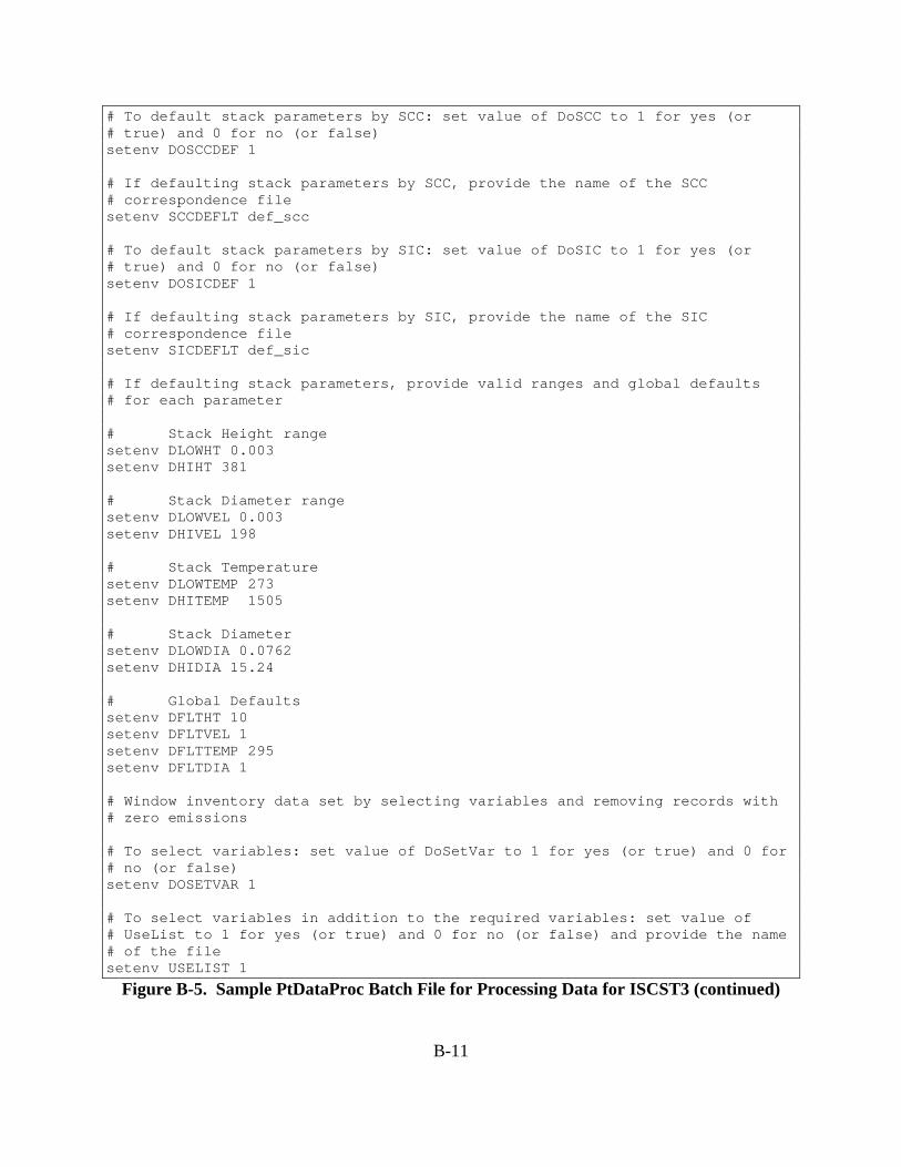
B-11
# To default stack parameters by SCC: set value of DoSCC to 1 for yes (or# true) and 0 for no (or false)setenv DOSCCDEF 1
# If defaulting stack parameters by SCC, provide the name of the SCC# correspondence filesetenv SCCDEFLT def_scc
# To default stack parameters by SIC: set value of DoSIC to 1 for yes (or# true) and 0 for no (or false)setenv DOSICDEF 1
# If defaulting stack parameters by SIC, provide the name of the SIC# correspondence filesetenv SICDEFLT def_sic
# If defaulting stack parameters, provide valid ranges and global defaults# for each parameter
# Stack Height rangesetenv DLOWHT 0.003setenv DHIHT 381
# Stack Diameter rangesetenv DLOWVEL 0.003setenv DHIVEL 198
# Stack Temperaturesetenv DLOWTEMP 273setenv DHITEMP 1505
# Stack Diametersetenv DLOWDIA 0.0762setenv DHIDIA 15.24
# Global Defaultssetenv DFLTHT 10setenv DFLTVEL 1setenv DFLTTEMP 295setenv DFLTDIA 1
# Window inventory data set by selecting variables and removing records with# zero emissions
# To select variables: set value of DoSetVar to 1 for yes (or true) and 0 for# no (or false)setenv DOSETVAR 1
# To select variables in addition to the required variables: set value of# UseList to 1 for yes (or true) and 0 for no (or false) and provide the name# of the filesetenv USELIST 1
Figure B-5. Sample PtDataProc Batch File for Processing Data for ISCST3 (continued)

B-12
setenv VARLIST varlist_philly
# To window by zero emissions and valid locations: set value of DoWindow to# 1 for yes (or true) and 0 for no (or false)setenv DOWINDOW 1
# If windowing inventory, provide names of data sets to store the records# with zero emissions and the records without lat/lon values.setenv NOLOCATE nolatlonsetenv ZEROEMIS zeroemis
cp -p /vail2aspen/dyntel/EMSHAP/PROGRAMS/V3/PtDataProc_V3.sas PtDataProc_PHILLY.sassas PtDataProc_PHILLY -work .
Figure B-5. Sample PtDataProc Batch File for Processing Data for ISCST3 (continued)

B-13
# Point Source Processing - Model Specific Processing
# Provide the Model for which the data is being processedsetenv MODEL ASPEN
# Provide directory paths:
# path for the SAS input data setsetenv IN_DATA /data/work16/EMSHAP/INVENTORY_NIF99/pt2003/
# path for the SAS output data setsetenv OUTDATA /data/work16/EMSHAP/INVENTORY_NIF99/pt2003/
# path for the reference SAS data setssetenv REFSAS /vail2aspen/dyntel/EMSHAP/ANCILLARY_NIF
# path for the reference text filessetenv REFTEXT /vail2aspen/dyntel/EMSHAP/ANCILLARY_NIF
# Provide input and output SAS data set names
# input SAS data set namesetenv INSAS dataproc
# output SAS data set namesetenv OUTSAS PtAspen
# Provide name of reference files containing pollutant information and# census tract information
# name of the text files containing the correspondence between the pollutant# code used in the inventory and CAS number, SAROAD code, NTI HAP code,# pollutant description and a flag indicating whether the pollutant should# be retained for processing
################################################################################ 3 HAP TABLE FILES######################################################################## 2 HAP-General Files: point-area & non-road########################################################################## General Non-Road HAP Tablesetenv G_MOBHAP haptabl_nonroadGEN_toxwt
### General Point-Area HAP Tablesetenv G_PTHAP haptabl_stationary_188########################################################################## Specific HAP Table. Applies to all inventories: May be "NONE"setenv SPECHAP haptabl_SPEC
# name of the sas data set containing the urban/rural flags by county# (value is 1 or 0 if all tracts within the county of the same and value is# 9 for non-uniform counties)
Figure B-6. Sample PtModelProc Batch File for Processing Data for ASPEN

B-14
setenv CTYFLAG ctyflag99
# name of the SAS data set containing the census tract information,# including urban/rural flags, state and county FIP codes, tract location,# and tract radiussetenv TRCTINF tractinf99
cp -p /vail2aspen/dyntel/EMSHAP/PROGRAMS/V3/PtModelProc_V3.sas PtModelProc_jul03.sassas PtModelProc_jul03 -work /data/work17/
Figure B-6. Sample PtModelProc Batch File for Processing Data for ASPEN (continued)
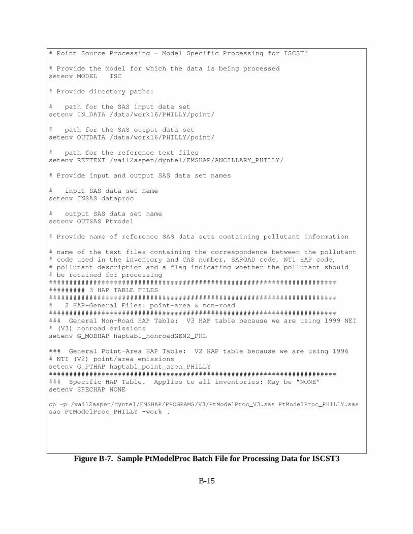
B-15
# Point Source Processing - Model Specific Processing for ISCST3
# Provide the Model for which the data is being processedsetenv MODEL ISC
# Provide directory paths:
# path for the SAS input data setsetenv IN_DATA /data/work16/PHILLY/point/
# path for the SAS output data setsetenv OUTDATA /data/work16/PHILLY/point/
# path for the reference text filessetenv REFTEXT /vail2aspen/dyntel/EMSHAP/ANCILLARY_PHILLY/
# Provide input and output SAS data set names
# input SAS data set namesetenv INSAS dataproc
# output SAS data set namesetenv OUTSAS Ptmodel
# Provide name of reference SAS data sets containing pollutant information
# name of the text files containing the correspondence between the pollutant# code used in the inventory and CAS number, SAROAD code, NTI HAP code,# pollutant description and a flag indicating whether the pollutant should# be retained for processing################################################################################ 3 HAP TABLE FILES######################################################################## 2 HAP-General Files: point-area & non-road########################################################################## General Non-Road HAP Table: V3 HAP table because we are using 1999 NEI# (V3) nonroad emissionssetenv G_MOBHAP haptabl_nonroadGEN2_PHL
### General Point-Area HAP Table: V2 HAP table because we are using 1996# NTI (V2) point/area emissionssetenv G_PTHAP haptabl_point_area_PHILLY########################################################################## Specific HAP Table. Applies to all inventories: May be "NONE"setenv SPECHAP NONE
cp -p /vail2aspen/dyntel/EMSHAP/PROGRAMS/V3/PtModelProc_V3.sas PtModelProc_PHILLY.sassas PtModelProc_PHILLY -work .
Figure B-7. Sample PtModelProc Batch File for Processing Data for ISCST3

B-16
# Point Source Processing - Temporal V3 1999 NEI
# Provide the Model for which the data is being processed (ASPEN or ISC)setenv MODEL ASPEN
# Provide directory paths:
# path for the SAS input data setsetenv IN_DATA /data/work16/EMSHAP/INVENTORY_NIF99/pt2003
# path for the SAS output data setsetenv OUTDATA /data/work16/EMSHAP/INVENTORY_NIF99/pt2003
# path for the reference text filessetenv REFFILE /vail2aspen/dyntel/EMSHAP/ANCILLARY_NIF
# Provide input and output SAS data set names
# input SAS data set namesetenv INSAS PtAspen
# output SAS data set namesetenv OUTSAS Temporal
# Provide name of Temporal Allocation File (TAF)setenv TAF taff_hourlyV3dpmPRE
# Provide name of the SCC_AMS correspondence texts:
# name of SCC to SCC_AMS correspondence filesetenv SCCLINK scc2amsV3
# name of SIC to SCC_AMS correspondence filesetenv SICLINK sic2scc
# name of MACT category code to SCC_AMS correspondence filesetenv MACTLINK mact2scc
cp -p /vail2aspen/dyntel/EMSHAP/PROGRAMS/V3/PtTemporal_V3.sas PtTemporal_jul03.sassas PtTemporal_jul03 -work /data/work17
Figure B-8. Sample PtTemporal Batch File for Processing Data for ASPEN

B-17
# ONROAD MOBILE6 ROAD SEGMENTS -USES ARRAY OF EMISSIONS for SUMMER AND WINTER
# Provide the Model for which the data is being processed (ASPEN or ISC)setenv MODEL ISC
# For ISCST3, conservation of annual emissions depends on number of days.# Leap year: 1=yes, 0= nosetenv LEAPYEAR 1
# Provide directory paths:
# path for the SAS input data setsetenv IN_DATA /data/work16/PHILLY/ONROAD_SEGMENTS/MARCH2003/
# path for the SAS output data setsetenv OUTDATA /data/work16/PHILLY/ONROAD_SEGMENTS/MARCH2003/
# path for the reference text filessetenv REFFILE /vail2aspen/dyntel/EMSHAP/ANCILLARY_PHILLY/
# Provide input and output SAS data set names
# input SAS data set namesetenv INSAS mob6_temporal_inpnew
# output SAS data set namesetenv OUTSAS Temporal_mob6new
# Provide name of Temporal Allocation File (TAF)setenv TAF taff-ISCfactorsV3_mob6
# Provide name of the SCC_AMS correspondence texts:
# name of SCC to SCC_AMS correspondence filesetenv SCCLINK scc2amsV3
# name of SIC to SCC_AMS correspondence filesetenv SICLINK sic2scc_philly
# name of MACT category code to SCC_AMS correspondence filesetenv MACTLINK mact2scc
cp -p /vail2aspen/dyntel/EMSHAP/PROGRAMS/V3/PtTemporal_V3.sas PtTemporal_MOBIL62new.sas
sas PtTemporal_MOBIL62new -work .
Figure B-9. Sample PtTemporal Batch File for Processing Data for ISCST3

B-18
#Point Source Processing - The Growth and Control Program (PtGrowCntl)
# Model for which EMS-HAP is being run: ASPEN or ISCsetenv MODEL ASPEN
#Provide directory paths:
# path for the SAS input datasetssetenv IN_DATA /data/work16/EMSHAP/INVENTORY_NIF99/PROJ/pt/
# path for the SAS output datasetssetenv OUTDATA /data/work16/EMSHAP/INVENTORY_NIF99/PROJ/pt/OUTP/
# path for the reference text filessetenv REFTEXT /vail2aspen/dyntel/EMSHAP/ANCILLARY_V3/
#Provide input and output SAS data set names:
# input SAS data set namesetenv INSAS temporal188_fixsic
# GROWTH and CONTROL: set to NONE or leave blank if you are not projectingsetenv PROJECT proj_NIF99_ptV3
# output SAS data set prefix:# remainder of the filename appended w/ column K text in PROJECT spreadsheetsetenv OUTSAS pt188_
cp -p /vail2aspen/dyntel/EMSHAP/PROGRAMS/V3/PtGrowCntl_V3.sas PtGrowCntl_NIF99.sassas PtGrowCntl_NIF99 -work .
Figure B-10. Sample PtGrowCntl Batch File for Processing Data for ASPEN

B-19
#Point Source Processing - Final Format# Assigns source groups for ASPEN# Produces ASPEN-formatted text files
# Provide the Model for which data is being processed (ASPEN only)setenv MODEL ASPEN
# Provide directory paths:
# path for the SAS input datasetsetenv IN_DATA /data/work16/EMSHAP/INVENTORY_NIF99/pt2003
# path for the SAS output datasetsetenv OUTDATA /data/work16/EMSHAP/INVENTORY_NIF99/pt2003/ASPENemis/
# path for the reference text filessetenv REFFILES /vail2aspen/dyntel/EMSHAP/ANCILLARY_NIF
# path for the output files for input into ASPENsetenv OUTFILES /data/work16/EMSHAP/INVENTORY_NIF99/pt2003/ASPENemis/
# path for the single ASCII output filesetenv ASCIIFILE /data/work16/EMSHAP/INVENTORY_NIF99/pt2003/ASPENemis/
# Provide input and output SAS data set names# input SAS data set namesetenv INSAS temporal
# output SAS dataset namesetenv OUTSAS pt99_aug05
# Select the procedure to be used to assign source groups# Set value to 1 for yes (or true) and 0 for no (or false)
# Assign source groups by source type (major or area): set value of DoSource# to 1 for yes (or true) and 0 for no (or false)setenv DOSOURCE 1
# Assign source groups by MACT categories: set value of DoMACT to 1 for yes# (or true) and 0 for no (or false)setenv DOMACT 0
# If using MACT categories, provide name of the text file containing the# group assignmentssetenv MACTGRP MACT_grp
# Assign source groups by SCCs: set value of DoSCC to 1 for yes (or true)# and 0 for no (or false)setenv DOSCC 0
Figure B-11. Sample PtFinal_ASPEN Batch File for Processing Data for ASPEN

B-20
# If using SCCs, provide the name of the text file containing the group# assignmentssetenv SCCGRP SCC_grp
# Assign source groups by SIC: set value of DoSIC to 1 for yes (or true)# and 0 for no (or false)setenv DOSIC 0
# If using SICs, provide the name of the text file containing the group# assignmentssetenv SICGRP SIC_grp
# Provide a default group assignment (value between 0 and 9) for those# sources not assigned by your selected proceduresetenv DFLTGRP 1
# Select the creation of ASPEN-formatted text files# Set value of DoWrite to 1 for yes (or true) and 0 for no (or false)setenv DOWRITE 1
# Provide the file name of the text file containing the decay rates for each# reactivity class, extension must be .txtsetenv DECAY indecay
# Provide a file identifier (maximum of 10 character) to be included in the# name of the ASPEN-formatted text filessetenv OUTCODE PT99_aug05
# Specify the source type, set value of Itype to 0 for point sources and 3# for pseudo point sourcessetenv ITYPE 0
# Provide an identifying run name to be included in the file header (maximum# of 25 characters)setenv RUNID 'NIF POINT JUL03'
# Select the creation of the single ASCII-formatted file# Set value of DoASCII to 1 for yes (or true) and 0 for no (or false)setenv DOASCII 1
# Provide the file name of the output ASCII filesetenv ASCII PT99_aug05
cp -p /vail2aspen/dyntel/EMSHAP/PROGRAMS/V3/PtFinal_ASPEN_V3.sas PtFinal_ASPEN_jul03.sas
sas PtFinal_ASPEN_jul03 -work /data/work17/
Figure B-11. Sample PtFinal_ASPEN Batch File for Processing Data for ASPEN
(continued)

B-21
#Point Source Processing - Final Format - For ISCST3 data Processing# Assigns source groups for ISCST3# Produces ISCST3 - formatted text files
# Provide the model for which the data is being processed (must be ISC)setenv MODEL ISC
# Provide 1-character model-run identifier. This ensures that ISCST3# contains unique source ID's when all EMS-HAP output are fed into it.# "M"OBIL6.2 2003 RUNsetenv RUN_ID M
# Provide directory paths:
# path for the SAS input datasetsetenv IN_DATA /data/work16/PHILLY/ONROAD_SEGMENTS/MARCH2003/
# path for the SAS output datasetsetenv OUTDATA /data/work16/PHILLY/ONROAD_SEGMENTS/MARCH2003/
# path for the reference text filessetenv REFFILES /vail2aspen/dyntel/EMSHAP/ANCILLARY_PHILLY/
# path for the output files for input into ASPEN or ISCsetenv OUTFILES /data/work16/PHILLY/ONROAD_SEGMENTS/MARCH2003/ISCemis/
# Provide input and output SAS data set names
# input SAS data set namesetenv INSAS temporal_mob6new
# output SAS dataset namesetenv OUTSAS isc_mob6new
# Select the procedure to be used to assign source groups# Set value to 1 for yes (or true) and 0 for no (or false)
# Assign source groups by source type (major or area): set value of DoSource# to 1 for yes (or true) and 0 for no (or false)setenv DOSOURCE 1
# Assign source groups by MACT categories: set value of DoMACT to 1 for yes# (or true) and 0 for no (or false)setenv DOMACT 0
# If using MACT categories, provide name of the text file containing the# group assignmentssetenv MACTGRP MACT_grp
# Assign source groups by SCCs: set value of DoSCC to 1 for yes (or true)# and 0 for no (or false)setenv DOSCC 0
Figure B-12. Sample PtFinal_ISCST3 Batch File for Processing Data for ISCST3

B-22
# If using SCCs, provide the name of the text file containing the group# assignmentssetenv SCCGRP SCC6_grp
# Assign source groups by SIC: set value of DoSIC to 1 for yes (or true) and# 0 for no (or false)setenv DOSIC 0
# If using SICs, provide the name of the text file containing the group# assignmentssetenv SICGRP SIC_grp
# Provide a default group assignment (value between 00 and 99) for those# sources not assigned by your selected proceduresetenv DFLTGRP 01
# Provide ancillary file that contains default particle distributions:# SAROAD, # of sizes, list of size distributions, list of mass fractions,# list of densities, and liquid scaveng.setenv DEFPART defpartPHILLY
# SCC-specific particle distribution file -put "NONE" if it doesn't existsetenv SCCPART NONE
# Provide ancillary file that contains default gas deposition parameters:# SAROAD, diffusivity, alphas, Reac, Rsubm, Henry's coefficientsetenv DEFGAS defgasPHILLY
# Set to yes(1) if you want to use scavenging coefficients that may be# included in DEFPART and DEFGAS filessetenv SCAVENG 1
# grid cell elevation datasetenv ELEVDAT philly-elev
# default elevation in meters (used only if ELEVDAT does not exist)setenv DEFELEV 100
# Set to yes (1) to call the macro that writes the building dimension# include filessetenv USEBLDG 0
# Provide Southwest corner UTM coordinates (X_ORIG,YORIG) and number of 1x1# km columns and rows# SEE G:/USER/SHARE/PAL/PHILLY/Philly_ISCST3prep_JUL29.docsetenv X_ORIG 432000setenv Y_ORIG 4369000setenv CELLSIZE 1000setenv MAXCOL 107setenv MAXROW 107
Figure B-12. Sample PtFinal_ISCST3 Batch File for Processing Data for ISCST3 (continued)

B-23
# Part of run-stream for ISC inputsetenv OUTNAME PHL_MOB6new
# Write particle distribution include files: 1 = particle data by source,# 2 = particle data by pollutantsetenv PARTMETH 2
cp -p /vail2aspen/dyntel/EMSHAP/PROGRAMS/V3/PtFinal_ISCST3_V3.sas PtFinal_ISCST3_MOB62new.sas
sas PtFinal_ISCST3_MOB62new -work .
Figure B-12. Sample PtFinal_ISCST3 Batch File for Processing Data for ISCST3
(continued)

B-24
# Assigns source groups for ISCST3# Produces ISCST3 - formatted text files
# Provide the model for which the data is being processed (must be ISC)setenv MODEL ISCTRACT
# Provide 1-character model-run identifier. This ensures that ISCST3# contains unique source ID's when all EMS-HAP output are fed into it.# "M"OBIL6.2 2003 RUNsetenv RUN_ID M
# Provide directory paths:
# path for the SAS input datasetsetenv IN_DATA /data/work16/PHILLY/ONROAD_SEGMENTS/MARCH2003/
# path for the SAS output datasetsetenv OUTDATA /data/work16/PHILLY/ONROAD_SEGMENTS/MARCH2003/
# path for the reference SAS filessetenv REFFILES /vail2aspen/dyntel/EMSHAP/ANCILLARY_PHILLY/
# path for the reference text filessetenv REFFILES /vail2aspen/dyntel/EMSHAP/ANCILLARY_PHILLY/
# path for the output files for input into ASPEN or ISCsetenv OUTFILES /data/work16/PHILLY/ONROAD_SEGMENTS/MARCH2003/ISCemis/
# Provide input and output SAS data set names
# input SAS data set namesetenv INSAS temporal_mob6new
# output SAS dataset namesetenv OUTSAS isc_mob6new
# Select the procedure to be used to assign source groups# Set value to 1 for yes (or true) and 0 for no (or false)
# Assign source groups by source type (major or area): set value of DoSource# to 1 for yes (or true) and 0 for no (or false)setenv DOSOURCE 1
# Assign source groups by MACT categories: set value of DoMACT to 1 for yes# (or true) and 0 for no (or false)setenv DOMACT 0
# If using MACT categories, provide name of the text file containing the# group assignmentssetenv MACTGRP MACT_grp
Figure B-13. Sample PtFinal_ISCST3 Batch File for Processing Data for ISCST3 Using Tract-level Elevation Data

B-25
# Assign source groups by SCCs: set value of DoSCC to 1 for yes (or true)# and 0 for no (or false)setenv DOSCC 0
# If using SCCs, provide the name of the text file containing the group# assignmentssetenv SCCGRP SCC6_grp
# Assign source groups by SIC: set value of DoSIC to 1 for yes (or true) and# 0 for no (or false)setenv DOSIC 0
# If using SICs, provide the name of the text file containing the group# assignmentssetenv SICGRP SIC_grp
# Provide a default group assignment (value between 00 and 99) for those# sources not assigned by your selected proceduresetenv DFLTGRP 01
# Provide ancillary file that contains default particle distributions:# SAROAD, # of sizes, list of size distributions, list of mass fractions,# list of densities, and liquid scaveng.setenv DEFPART defpartPHILLY
# SCC-specific particle distribution file -put "NONE" if it doesn't existsetenv SCCPART NONE
# Provide ancillary file that contains default gas deposition parameters:# SAROAD, diffusivity, alphas, Reac, Rsubm, Henry's coefficientsetenv DEFGAS defgasPHILLY
# Set to yes(1) if you want to use scavenging coefficients that may be# included in DEFPART and DEFGAS filessetenv SCAVENG 1
# grid cell elevation datasetenv ELEVDAT tract-elev
# default elevation in meters (used only if ELEVDAT does not exist)setenv DEFELEV 100
# Set to yes (1) to call the macro that writes the building dimension# include filessetenv USEBLDG 0# Provide Southwest corner UTM coordinates (X_ORIG,YORIG) and number of 1x1# km columns and rows# SEE G:/USER/SHARE/PAL/PHILLY/Philly_ISCST3prep_JUL29.docsetenv X_ORIG 432000setenv Y_ORIG 4369000setenv CELLSIZE
Figure B-13. Sample PtFinal_ISCST3 Batch File for Processing Data for ISCST3 Using Tract-level Elevation Data (continued)

B-26
setenv MAXCOLsetenv MAXROW# give name of tract info file and UTM zonesetenv TRCTINF tractinf99setenv REF_ZONE 18# Part of run-stream for ISC inputsetenv OUTNAME PHL_MOB6new
# Write particle distribution include files: 1 = particle data by source,# 2 = particle data by pollutantsetenv PARTMETH 2
cp -p /vail2aspen/dyntel/EMSHAP/PROGRAMS/V3/PtFinal_ISCST3_V3.sas PtFinal_ISCST3_MOB62new.sas
sas PtFinal_ISCST3_MOB62new -work .
Figure B-13. Sample PtFinal_ISCST3 Batch File for Processing Data for ISCST3 Using Tract-level Elevation Data (continued)

B-27
# CountyProc: NIF3.0 Non-point
#Provide model for which the data is being processed (ASPEN or ISC)setenv MODEL ASPEN
# Indicate whether you want a 'diet' run or not (1=YES, 0=NO)# extended SAS data will NOT be created if DIET option is chosensetenv DIET 1
# CountyProc RUN IDENTIFICATION INFORMATION# Run identification for titlessetenv RUNID 'NIF 3.0 1999 Non-Point Emissions';
# Description of emissions filesetenv EMISLABL 'NIF 3.0 1999 Non-Point Emissions';
# Date identifying this runsetenv RUNDATE 082903
# Emissions type (AR for area, MV for mobile)setenv EMISTYPE AR
# Label for output filessetenv USRLABEL nonpt
# FILE DIRECTORIES# Ancillary files directorysetenv INPFILES /vail2aspen/dyntel/EMSHAP/ANCILLARY_NIF/
# Input emissions file directorysetenv INPEMISS /data/work16/EMSHAP/INVENTORY_NIF99/np2003/
# Output files directorysetenv OUTFILES /data/work16/EMSHAP/INVENTORY_NIF99/np2003/ASPENemis/
# INPUT FILES# Input emissions file name prefixsetenv EMISFILE nonpt99_aspen_ap
# SAF file name prefixsetenv SAFFILE SAFe
# Default SAF applied when SAF information missing for a county w/ emissionssetenv DEFLTSAF 100
# TAF file name prefixsetenv TAFFILE taff_hourlyV3dpmPRE
# Decay rates file name prefixsetenv INDECAY indecay################################################################################ 2 HAP TABLE FILES
Figure B-14. Sample CountyProc Batch File for Processing Data for ASPEN

B-28
######################################################################## HAP-General File########################################################################## General HAP Tablesetenv GENHAP haptabl_stationary_188########################################################################## Specific HAP Table. May be "NONE"#######################################################################setenv SPECHAP haptabl_SPEC#######################################################################
# Spatial surrogate xref file name prefixsetenv SURRXREF surrxref99
# Spatial surrogate to surrogate description xref prefix# (CSV -comma delimited): OPTIONAL inputsetenv SURRDESC surrogate_codes_and_definitions
# Emissions bins file name prefix: Format depends on inventorysetenv EMISBINS am_grp99PRE
# County urban/rural flag xref file name prefixsetenv CNTYUR popflg99
# GROWTH and CONTROL: set to NONE or leave blank if you are not projectingsetenv PROJECT NONE
# QA and OUTPUT FILES# Lsubsetp = 1 to subset to a pollutantsetenv LSUBSETP 0
# The pollutant code for subsetting tosetenv SUBSETP 98
# Lsubsetg = 1 to subset to a statesetenv LSUBSETG 0
# The 2-character state abbreviation for subsetting tosetenv SUBSETG US
# Ldbg = 1 to turn on debugging printssetenv LDBG 0
# The cell for debug prints (state|county|tract)setenv ONECELL 41019010098
# Assign temporary work space directorysetenv WORK2 /data/work17/
cp -p /vail2aspen/dyntel/EMSHAP/PROGRAMS/V3/CountyProc.sas CountyProc_nonpt.sastime sas CountyProc_nonpt -work /data/work17
Figure B-14. Sample CountyProc Batch File for Processing Data for ASPEN (continued)

B-29
# CountyProc batch file --- ISCST3 no GC
# Indicate whether you want a 'diet' run or not (Y=1, N=0)setenv DIET 1
#Provide model for which the data is being processed (ASPEN or ISC)setenv MODEL ISC
# For ISCST3, conservation of annual emissions depends on number of days.# Leap year: 1=yes, 0= nosetenv LEAPYEAR 1
# CountyProc RUN IDENTIFICATION INFORMATION# Run identification for titlessetenv RUNID 'EMS-HAP 1996 NEWNTI PHILLY NONROAD'
# Description of emissions filesetenv EMISLABL 'NEW1996 PHILLY NONROAD'
# Date identifying this runsetenv RUNDATE 073003
# Emissions type (AR for area, MV for mobile)setenv EMISTYPE MV
# Label for output filessetenv USRLABEL PHL
# FILE DIRECTORIES# Ancillary files directorysetenv INPFILES /vail2aspen/dyntel/EMSHAP/ANCILLARY_PHILLY/
# Input emissions file directorysetenv INPEMISS /data/work16/PHILLY/
# Output files directorysetenv OUTFILES /data/work16/PHILLY/NONROAD/
# INPUT FILES# Input emissions file name prefixsetenv EMISFILE mob_no_ap
# SAF file name prefixsetenv SAFFILE psaf
# Default SAF applied when SAF information missing for a county w/ emissionssetenv DEFLTSAF 20# TAF file name prefixsetenv TAFFILE taff-ISCfactorsV3_mob6
################################################################################ 2 HAP TABLE FILES
Figure B-15. Sample CountyProc Batch File for Processing Data for ISCST3

B-30
######################################################################## HAP-General File########################################################################## General HAP Tablesetenv GENHAP haptabl_nonroadGEN2_PHL########################################################################## Specific HAP Table. May be "NONE"#######################################################################setenv SPECHAP NONE#######################################################################
# Spatial surrogate xref file name prefixsetenv SURRXREF surrxref_philly_wNIF99mob
# Spatial surrogate to surrogate description xref prefix# (CSV -comma delimited): OPTIONAL inputsetenv SURRDESC
# Emissions bins file name prefixsetenv EMISBINS am_grp12NOV02
# County urban/rural flag xref file name prefix: for PHL, 1999 is the same# as 1996 (only format changed)setenv CNTYUR popflg99
# GROWTH and CONTROLsetenv PROJECT
# QA and OUTPUT FILES# Lsubsetp = 1 to subset to a pollutantsetenv LSUBSETP 0
# The pollutant code for subsetting tosetenv SUBSETP 98
# Lsubsetg = 1 to subset to a statesetenv LSUBSETG 0
# The 2-character state abbreviation for subsetting tosetenv SUBSETG US
# Ldbg = 1 to turn on debugging printssetenv LDBG 0
# The cell for debug prints (state|county|tract)setenv ONECELL 41019010098
# Assign temporary work space directorysetenv WORK2 ../
# Assign UTM-X origin of the modeling grid in meterssetenv XORIG 432000
Figure B-15. Sample CountyProc Batch File for Processing Data for ISCST3 (continued)

B-31
# Assign UTM-Y origin of the modeling grid in meterssetenv YORIG 4369000
# Assign the size (length) of each grid cell in meterssetenv CELLSIZE 1000
# Assign the prefix of the output SAS datasetsetenv ISCOUT cntyproc_nrd_out_diet1
cp /vail2aspen/dyntel/EMSHAP/PROGRAMS/V3/CountyProc.sas CountyProc_nonrd_PHILLY.sastime sas CountyProc_nonrd_PHILLY -work .
Figure B-15. Sample CountyProc Batch File for Processing Data for ISCST3 (continued)

B-32
# CountyProc batch file --- ISCST3 no GC
# Indicate whether you want a 'diet' run or not (Y=1, N=0)setenv DIET 1
#Provide model for which the data is being processed (ASPEN or ISC)setenv MODEL ISCTRACT
# For ISCST3, conservation of annual emissions depends on number of days.# Leap year: 1=yes, 0= nosetenv LEAPYEAR 1
# CountyProc RUN IDENTIFICATION INFORMATION# Run identification for titlessetenv RUNID 'EMS-HAP 1996 NEWNTI PHILLY NONROAD'
# Description of emissions filesetenv EMISLABL 'NEW1996 PHILLY NONROAD'
# Date identifying this runsetenv RUNDATE 073003
# Emissions type (AR for area, MV for mobile)setenv EMISTYPE MV
# Label for output filessetenv USRLABEL PHL
# FILE DIRECTORIES# Ancillary files directorysetenv INPFILES /vail2aspen/dyntel/EMSHAP/ANCILLARY_PHILLY/
# Input emissions file directorysetenv INPEMISS /data/work16/PHILLY/
# Output files directorysetenv OUTFILES /data/work16/PHILLY/NONROAD/
# INPUT FILES# Input emissions file name prefixsetenv EMISFILE mob_no_ap
# SAF file name prefixsetenv SAFFILE SAFe
# Default SAF applied when SAF information missing for a county w/ emissionssetenv DEFLTSAF 100# TAF file name prefixsetenv TAFFILE taff-ISCfactorsV3_mob6
################################################################################ 2 HAP TABLE FILES
Figure B-16. Sample CountyProc Batch File for Processing Data for ISCST3 Using Tract-Level Surrogates

B-33
######################################################################## HAP-General File########################################################################## General HAP Tablesetenv GENHAP haptabl_nonroadGEN2_PHL########################################################################## Specific HAP Table. May be "NONE"#######################################################################setenv SPECHAP NONE######################################################################## Spatial surrogate xref file name prefixsetenv SURRXREF surrxref_philly_wNIF99mob
# Spatial surrogate to surrogate description xref prefix# (CSV -comma delimited): OPTIONAL inputsetenv SURRDESC
# Emissions bins file name prefixsetenv EMISBINS am_grp12NOV02
# County urban/rural flag xref file name prefix: for PHL, 1999 is the same# as 1996 (only format changed)setenv CNTYUR popflg99
# GROWTH and CONTROLsetenv PROJECT
# QA and OUTPUT FILES# Lsubsetp = 1 to subset to a pollutantsetenv LSUBSETP 0
# The pollutant code for subsetting tosetenv SUBSETP 98
# Lsubsetg = 1 to subset to a statesetenv LSUBSETG 0
# The 2-character state abbreviation for subsetting tosetenv SUBSETG US
# Ldbg = 1 to turn on debugging printssetenv LDBG 0
# The cell for debug prints (state|county|tract)setenv ONECELL 41019010098
# Assign temporary work space directorysetenv WORK2 ../
# Assign UTM-X origin of the modeling grid in meterssetenv XORIG
Figure B-16. Sample CountyProc Batch File for Processing Data for ISCST3 Using Tract-Level Surrogates (continued)

B-34
# Assign UTM-Y origin of the modeling grid in meterssetenv YORIG# Assign the size (length) of each grid cell in meterssetenv CELLSIZE# Assign the prefix of the output SAS datasetsetenv ISCOUT cntyproc_nrd_out_diet1
cp /vail2aspen/dyntel/EMSHAP/PROGRAMS/V3/CountyProc.sas CountyProc_nonrd_PHILLY.sastime sas CountyProc_nonrd_PHILLY -work .
Figure B-16. Sample CountyProc Batch File for Processing Data for ISCST3 Using Tract-
Level Surrogates (continued)

B-35
# CountyFinal: ISCST3 GRIDDED AREA/MOBILE Source Processing - Final Format# Produces ISC -formatted text files# Provide Model Namesetenv MODEL ISC# Provide 1-character model-run identifier. This ensures that ISCST3# contains unique source ID's when all EMS-HAP output are fed into it.# A = Area (non-point) with NO airports -airports are processed separately# -see COPAX-nonroad batch filesetenv RUN_ID A
# Provide directory paths:
# path for the SAS input datasetsetenv IN_DATA /data/work16/PHILLY99/non-point/
# path for the SAS output datasetsetenv OUTDATA /data/work16/PHILLY99/non-point/
# path for the reference text filessetenv REFFILES /vail2aspen/dyntel/EMSHAP/ANCILLARY_PHILLY99/
# path for the output files for input into ISCsetenv OUTFILES /data/work16/PHILLY99/non-point/ISCemis/
# Provide input and output SAS data set names
# input SAS data set namesetenv INSAS countyproc_nonpt99_outp
# output SAS dataset namesetenv OUTSAS nonpt_grid_philly99
# Provide ancillary file that contains default particle distributions:# SAROAD, # of sizes, list of size distributions, list of mass fractions,# list of densities, and liquid scavenging# put "NONE" or leave blank if it does not exist is not desiredsetenv DEFPART defpartPHILLY
# Provide ancillary file that contains default gas deposition parameters:# SAROAD, diffusivity, alphas, Rx, Rsubm, Henry's coefficient# put "NONE" or leave blank if it does not exist is not desiredsetenv DEFGAS defgasPHILLY
# Set to yes (1) if you want to use scavenging coefficients that may be# included in DEFPART and DEFGAS filessetenv SCAVENG 1
# grid cell elevation data# put "NONE" or leave blank if it does not exist is not desiredsetenv ELEVDAT philly-elev
# default elevation in meters (used only if ELEVDAT does not exist)setenv DEFELEV 100
Figure B-17. Sample CountyFinal Batch File for Processing Data for ISCST3

B-36
# Provide Southwest corner UTM coordinates (X_ORIG,YORIG) and number of 1x1# km columns and rowssetenv X_ORIG 432000setenv Y_ORIG 4369000setenv CELLSIZE 1000setenv MAXCOL 107setenv MAXROW 107
# name of tract file with vertices for ISCTRACTsetenv TRACTFILE
# Reference UTM zonesetenv REF_ZONE
# area source release heights in meterssetenv ARELHGT 2
# initial vertical dimension of the area source plume in meterssetenv AINPLUM 1
cp -p /vail2aspen/dyntel/EMSHAP/PROGRAMS/V3/CountyFinal.sas CountyFinal_PHLnonpt99.sas
sas CountyFinal_PHLnonpt99 -work .
Figure B-17. Sample CountyFinal Batch File for Processing Data for ISCST3 (continued)

B-37
# CountyFinal: ISCTRACT AREA/MOBILE Source Processing - Final Format# Produces ISC -formatted text files# Provide Model Namesetenv MODEL ISCTRACT# Provide 1-character model-run identifier. This ensures that ISCST3# contains unique source ID's when all EMS-HAP output are fed into it.# A = Area (non-point) with NO airports -airports are processed separately# -see COPAX-nonroad batch filesetenv RUN_ID A
# Provide directory paths:
# path for the SAS input datasetsetenv IN_DATA /data/work16/PHILLY99/non-point/
# path for the SAS output datasetsetenv OUTDATA /data/work16/PHILLY99/non-point/
# path for the reference text filessetenv REFFILES /vail2aspen/dyntel/EMSHAP/ANCILLARY_PHILLY99/
# path for the output files for input into ISCsetenv OUTFILES /data/work16/PHILLY99/non-point/ISCemis/
# Provide input and output SAS data set names
# input SAS data set namesetenv INSAS countyproc_nonpt99_outp
# output SAS dataset namesetenv OUTSAS nonpt_grid_philly99
# Provide ancillary file that contains default particle distributions:# SAROAD, # of sizes, list of size distributions, list of mass fractions,# list of densities, and liquid scavenging# put "NONE" or leave blank if it does not exist is not desiredsetenv DEFPART defpartPHILLY
# Provide ancillary file that contains default gas deposition parameters:# SAROAD, diffusivity, alphas, Rx, Rsubm, Henry's coefficient# put "NONE" or leave blank if it does not exist is not desiredsetenv DEFGAS defgasPHILLY
# Set to yes (1) if you want to use scavenging coefficients that may be# included in DEFPART and DEFGAS filessetenv SCAVENG 1
# grid cell elevation data# put "NONE" or leave blank if it does not exist is not desiredsetenv ELEVDAT philly-elev# default elevation in meters (used only if ELEVDAT does not exist)setenv DEFELEV 100
Figure B-18. Sample CountyFinal Batch File for Processing Data for ISCST3 Using Tract-Level Emissions

B-38
# Provide Southwest corner UTM coordinates (X_ORIG,YORIG) and number of 1x1# km columns and rowssetenv X_ORIG 432000setenv Y_ORIG 4369000setenv CELLSIZEsetenv MAXCOLsetenv MAXROW
# name of tract file with vertices for ISCTRACTsetenv TRACTFILE tract_vertices
# Reference UTM zonesetenv REF_ZONE 17
# area source release heights in meterssetenv ARELHGT 2
# initial vertical dimension of the area source plume in meterssetenv AINPLUM 1
cp -p /vail2aspen/dyntel/EMSHAP/PROGRAMS/V3/CountyFinal.sas CountyFinal_PHLnonpt99.sas
sas CountyFinal_PHLnonpt99 -work .
Figure B-18. Sample CountyFinal Batch File for Processing Data for ISCST3 Using Tract-
Level Emissions (continued)

APPENDIX C
EMS-HAP ANCILLARY FILE DEVELOPMENT

C-ii
APPENDIX C ..................................................................................................................... i EMS-HAP Ancillary File Development .......................................................................................... i APPENDIX C EMS-HAP Ancillary File Development ................................................................ 1
C.1 Introduction ......................................................................................................................... 1 C.2 How we developed the Ancillary Files for COPAX ........................................................... 4
C.2.1 Allocation Extraction Files (keyword AP_AF): efm_apaf#.sas7bdat, where #=1, 2, 3, and 4 ........................................................................................................................................ 4 C.2.2 Allocation cross-reference file: airportxref99_OCT03.txt (keyword AIRPXREF) .. 12 C.2.3 Spatial Surrogates Assignment file: surrxref99.txt (keyword=SURRXREF).......... 12 C.2.4 How We Developed the Temporal Allocation Factor File (keyword TAFFILE ) ..... 30
C.3 How we developed the Ancillary Files for PtDataProc..................................................... 32 C.3.1 ASPEN-specific Ancillary Files Used to Quality Assure Point Source Data ............ 32 (Keywords ZIP, CNTYCENT, POLYGONS, MAP_INDX, TRACTS, TRCTINFO)......... 32 C.3.2 File Formats for the Stack Parameter Defaults........................................................... 34 C.3.3 Windowing the Inventory with the VARLIST file..................................................... 34
C.4 How we developed the Ancillary Files for PtModelProc.................................................. 35 C.4.1 Urban/Rural Flag files for ASPEN Processing (Keywords TRCTINF, CTYFLAG) 35 C.4.2 How we developed the General HAP Tables ............................................................. 35 C.4.3 How we developed the Specific HAP Table File (Keyword SPECHAP): haptabl_SPEC.txt .................................................................................................................. 59
C.5 How we developed the Ancillary Files for PtTemporal .................................................... 75 C.6 How we developed the Ancillary Files for PtGrowCntl ................................................... 75 C.7 How we developed the Ancillary Files for PtFinal_ASPEN............................................. 75 C.8 How we developed the Ancillary Files for PtFinal_ISCST3 and CountyFinal................. 76 C.9 How we developed the Ancillary Files for CountyProc.................................................... 78
C.9.1 How we developed the files for grouping sources (keywords EMISBINS and CNTYUR) ............................................................................................................................. 78 C.9.2 How we developed the files for spatial allocation (keywords SAFFILE and SURRDESC)......................................................................................................................... 78
This structure will cause a lot of referencing to previous sections. For example, the HAP tables will not be repeated in the CountyProc section; the temporal files will not be repeated in PtTemporal (as they are in COPAX)
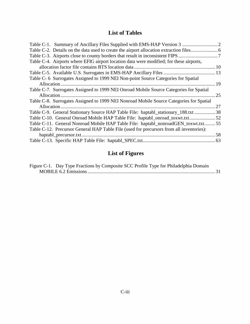
C-iii
List of Tables Table C-1. Summary of Ancillary Files Supplied with EMS-HAP Version 3 ............................. 2 Table C-2. Details on the data used to create the airport allocation extraction files...................... 6 Table C-3. Airports close to county borders that result in inconsistent FIPS ................................ 7 Table C-4. Airports where EFIG airport location data were modified; for these airports,
allocation factor file contains BTS location data .................................................................. 10 Table C-5. Available U.S. Surrogates in EMS-HAP Ancillary Files .......................................... 13 Table C- 6 Surrogates Assigned to 1999 NEI Non-point Source Categories for Spatial
Allocation .............................................................................................................................. 19 Table C-7. Surrogates Assigned to 1999 NEI Onroad Mobile Source Categories for Spatial
Allocation .............................................................................................................................. 25 Table C-8. Surrogates Assigned to 1999 NEI Nonroad Mobile Source Categories for Spatial
Allocation .............................................................................................................................. 27 Table C-9. General Stationary Source HAP Table File: haptabl_stationary_188.txt ................. 38 Table C-10. General Onroad Mobile HAP Table File: haptabl_onroad_toxwt.txt..................... 52 Table C-11. General Nonroad Mobile HAP Table File: haptabl_nonroadGEN_toxwt.txt......... 55 Table C-12. Precursor General HAP Table File (used for precursors from all inventories):
haptabl_precursor.txt............................................................................................................. 58 Table C-13. Specific HAP Table File: haptabl_SPEC.txt........................................................... 63
List of Figures
Figure C-1. Day Type Fractions by Composite SCC Profile Type for Philadelphia Domain
MOBILE 6.2 Emissions ........................................................................................................ 31

C-1
APPENDIX C EMS-HAP Ancillary File Development C.1 Introduction This appendix describes the development of each ancillary file supplied with EMS-HAP Version 3. It also contains complete listings and/or summaries of some of the key files such as the HAP tables and the surrogate cross-reference file. We supply all of the files you need process the 1999 NEI for a national scale assessment (i.e., running EMS-HAP for ASPEN). The ancillary filenames provided in each figure are based on data we used to process the version 3 final 1999 NEI through EMS-HAP for the National Scale Assessment modeling done in the fall of 2003 and in early 2004 (diesel PM was run several months after the hazardous air pollutants for this assessment). In the event we update these files in the future, we will post them on www.epa.gov/ttn/chief/emch. Many of the ancillary files are updated from those developed and used for the National Scale Assessment using the 1996 inventory (www.epa.gov/ttn/nata). As a result, one of the main references to this appendix is Appendix D of the EMS-HAP Version 2.0 User’s guide (EPA 454/B-02-001). Other references appear directly in the text, such that there is no separate reference section for this appendix. We also provide some of the ancillary files you can use for preparing emissions for an urban toxics study using the EMS-HAP/ISCST3 modeling system. We only provide files that are not domain-specific. For example, if you choose to model a particular 100 by 100 km domain using a 1 by 1 kilometer grid cell approach, we do not provide the spatial surrogate ratios (SAF files); you will have to generate these yourself. However, if you use the tract-level approach (new addition to EMS-HAP Version 3), then you can use the tract-level SAF files. The same ancillary files are often used in different EMS-HAP programs. We provide a discussion of their development only once. For example, the Temporal Allocation Factor (TAF) ancillary file is used in COPAX (Chapter 2), PtTemporal (Chapter 5), and CountyProc (Chapter 9); we discuss this file in Section C.1 (COPAX Ancillary Files) only. Use Table C-1 to find where each file supplied with EMS-HAP Version 3 is discussed. This appendix references only those files we supply with EMS-HAP Version 3. You may need to develop additional files for your specific application. Table C-1 lists the files we supply.
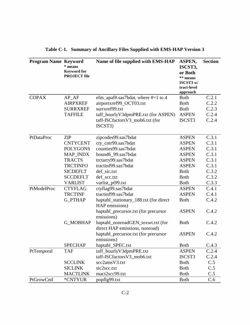
C-2
Table C-1. Summary of Ancillary Files Supplied with EMS-HAP Version 3
Program Name Keyword * means Keyword for PROJECT file
Name of file supplied with EMS-HAP ASPEN, ISCST3, or Both ** means ISCST3 w/ tract-level approach
Section
COPAX AP_AF efm_apaf#.sas7bdat, where #=1 to 4 Both C.2.1 AIRPXREF airportxref99_OCT03.txt Both C.2.2 SURRXREF surrxref99.txt Both C.2.3 taff_hourlyV3dpmPRE.txt (for ASPEN) ASPEN C.2.4
TAFFILE taff-ISCfactorsV3_mob6.txt (for ISCST3)
ISCST3 C.2.4
PtDataProc ZIP zipcodes99.sas7bdat ASPEN C.3.1 CNTYCENT cty_cntr99.sas7bdat ASPEN C.3.1 POLYGONS counties99.sas7bdat ASPEN C.3.1 MAP_INDX bound6_99.sas7bdat ASPEN C.3.1 TRACTS trctarry99.sas7bdat ASPEN C.3.1 TRCTINFO tractinf99.sas7bdat ASPEN C.3.1 SICDEFLT def_sic.txt Both C.3.2 SCCDEFLT def_scc.txt Both C.3.2 VARLIST varlist_pt99.txt Both C.3.3 PtModelProc CTYFLAG ctyflag99.sas7bdat ASPEN C.4.1 TRCTINF tractinf99.sas7bdat ASPEN C.4.1 haptabl_stationary_188.txt (for direct
HAP emissions) Both C.4.2
G_PTHAP
haptabl_precursor.txt (for precursor emissions)
ASPEN C.4.2
haptabl_nonroadGEN_toxwt.txt (for direct HAP emissions, nonroad)
Both C.4.2
G_MOBHAP
haptabl_precursor.txt (for precursor emissions)
ASPEN C.4.2
SPECHAP haptabl_SPEC.txt Both C.4.3 PtTemporal TAF taff_hourlyV3dpmPRE.txt ASPEN C.2.4 taff-ISCfactorsV3_mob6.txt ISCST3 C.2.4 SCCLINK scc2amsV3.txt Both C.5 SICLINK sic2scc.txt Both C.5 MACTLINK mact2scc99.txt Both C.5 PtGrowCntl *CNTYUR popflg99.txt Both C.6

C-3
Table C-1. Summary of Ancillary Files Supplied with EMS-HAP Version 3
Program Name Keyword * means Keyword for PROJECT file
Name of file supplied with EMS-HAP ASPEN, ISCST3, or Both ** means ISCST3 w/ tract-level approach
Section
PtFinal_ASPEN INDECAY indecay.txt ASPEN C.7 PtFinal_ISCST3 DEFPART defpartPHILLY.txt ISCST3 C.8 DEFGAS defgasPHILLY.txt ISCST3 C.8 TRCTINF tractinf99.sas7bdat ISCST3** C.4.1 ELEVDAT tract-elev.txt ISCST3** C.8 CountyProc haptabl_stationary_188.txt (for direct
HAP emissions) Both C.4.2
haptabl_nonroadGEN_toxwt.txt (for direct HAP emissions, nonroad)
Both C.4.2
haptabl_onroad_toxwt.txt (for direct HAP emissions, onroad)
Both C.4.2
GENHAP
haptabl_precursor.txt (for precursor emissions any source)
ASPEN C.4.2
SPECHAP haptabl_SPEC.txt Both C.4.3 EMISBINS am_grp99PRE.txt Both C.9.1 CNTYUR popflg99.txt Both C.6.3 SURRXREF surrxref99.txt Both C.2.3 SAFFILE safe#.sas7bdata, where # is each 3 digit
value shown in Table C-5 ASPEN C.9.2
SURRDESC surrogate_codes_and_definitions.csv Both C.9.2 taff_hourlyV3dpmPRE.txt ASPEN C.2.4
TAFFILE taff-ISCfactorsV3_mob6.txt ISCST3 C.2.4
INDECAY indecay.txt ASPEN C.7 *CNTYUR popflg99.txt Both C.6 CountyFinal DEFPART defpartPHILLY.txt ISCST3 C.8 DEFGAS defgasPHILLY.txt ISCST3 C.8 TRACTFILE Tract_vertices_xx.sas7bdat where xx is
the 2 letter abbreviation for each of the conterminous 48 U. S. states and DC
ISCST3** C.8
ELEVDAT tract-elev.txt ISCST3** C.8 a if you use the updated ports (SAF=800) and/or updated navigable waterways (SAF=810) the files have the prefix “safdi” instead of “safe”. To use the remaining surrogates with the new surrogates, the remaining surrogate files must be copied to files with the prefix “safdi”. If you do not want to use the new ports and navigable waterways, you do not have to copy the remaining surrogate files and the older ports and navigable waterways will be used.

C-4
C.2 How we developed the Ancillary Files for COPAX
The files we supply with EMS-HAP Version 3 allow you to perform a number of COPAX’s functions for processing 1999 NEI data. The allocation extraction and allocation cross reference files discussed in C.2.1 and C.2.2 allow you to extract airport-related emissions from the non-point and nonroad inventories and allocate them to airport locations based on activity data. The surrogate cross-reference file allows surrogates to be assigned to non-point sources in preparation for running CountyProc for non-point sources. The temporal allocation profile files allow for COPAX to give you information on the temporal allocation of your non-point inventory for either the ASPEN or ISCST3 model. The particular files are presented in the sections below.
C.2.1 Allocation Extraction Files (keyword AP_AF): efm_apaf#.sas7bdat, where #=1, 2, 3, and 4
We supply four allocation extraction files with EMS-HAP to allow you to model your airport-related emissions such as commercial aircraft (SCC= 2275020000) at the locations of airports in your domain.
Airport Allocation Filename Allocation factor based on activity of:
efm_apaf 1.sas7bdat General aircraft efm_apaf 2.sas7bdat Commercial aircraft efm_apaf 3.sas7bdat Air taxi efm_apaf 4.sas7bdat Military aircraft
The keyword AP_AF = “efm_apaf” for these files. The numeric value after the efm_apaf is associated with a code supplied by the allocation cross-reference file discussed in the next section (C.2.2). This code is 1, 2, 3, or 4 and its value represents the source of activity for the allocation factor data shown above. The efm_apaf files supplied with EMS-HAP Version 3 contain airports in the U.S., Puerto Rico and the Virgin Islands. Each of the four files contains exactly the same airports. For each airport, the file contains the associated geographic coordinates (latitude, longitude, in decimal degrees), FIPs code and an airport allocation factor to go from county-level emissions to airport-level emissions. In addition, there are other fields to identify the airport and provide additional information about the data sources. The allocation factor is based on airport activity: number or itinerant operations for the year 1999, for the particular type of aircraft, where available. Itinerant operations are defined as aircraft take-offs whereby the aircraft leaves the airport vicinity and lands at another airport, or aircraft landings whereby the aircraft has arrived from outside the airport vicinity. We computed the allocation factor for each of the aircraft operations from the itinerant data for each of these

C-5
operations for each airport. For example, for an airport, I, the factor for general aviation is computed as:
Factor I, GA = IT GA, I / IT GA, county
where:
Factor I, GA = allocation factor for airport I, for general aviation emissions
IT GA, I = itinerant data for general aviation for airport I
IT GA, county j = itinerant data for general aviation for all airports in the county where airport I resides
If the county sum of all itinerant data for general aviation is zero, commercial allocation factors are used in the file. If the county sum of all commercial itinerant data is zero, general aviation, then air taxi, then military allocation factors, are used. If the county sum of military or air taxi itinerant data is zero, general aviation allocation factors are used. Finally, if itinerant data are not available for any of the airports in a particular county, then the allocation factor is equal to 1 divided by the number of airports in that county. This data substitution ensures that the county sum for each of the four aircraft allocation factors equal unity (1). We utilized itinerant and airport location data from three sources: (1) EFIG (Emission Factor and Inventory Group) airport data: Itinerant and location data
for approximately 2000 airports. This is the file that the EFIG used to develop EPA estimates of aircraft emissions for the 1999 NEI. We corrected some of the location data in this file as described further below.
(2) TAF data: Itinerant data for approximately 3400 airports. Data obtained from running the Federal Aviation Administration (FAA) Terminal Area Forecast (TAF) model. For the TAF airports, we merged locations (latitudes/longitudes) from the Bureau of Transportation Statistics National Transportation Atlas Data (BTS), item 3 below, and we used a geographic information system (GIS) to determine the FIPS codes.
(3) BTS data: Airport location data for about 20,000 airports. We used GIS to determine the FIPS codes.
More details on the above three datasets are presented in Table C-2. We used the following hierarchy:
• For counties for which the EFIG dataset contains at least one airport, we used the EFIG airport data only.
• For counties having no EFIG airports, we used airports in the TAF data only. • For counties having no airports from either of the above, we used airports listed in the
BTS. For each of these counties, if the BTS had multiple airports listed, each airport received the same allocation factor for the various types of aviation (1/number of airports in the county).

C-6
Note that with this hierarchy, if the EFIG data contained two airports for a particular county, and the TAF data showed a third airport for that county, then the third airport will not be present in the allocation file.
Table C-2. Details on the data used to create the airport allocation extraction files
1) EFIG airport data: Airport database developed by the Emission Factor and Inventory Group (EFIG), supplied as auxiliary data with the inventory for the 1999 NEI for HAPs, version 3. Data are contained in county_air.mdb, which is contained in gis_data.zip, available at: ftp://ftp.epa.gov/pub/EmisInventory/finalnei99ver3/haps/datafiles/nonroad/auxiliary/ (accessed October, 2003). This database contains a list of each airport for which emissions were computed by EPA (it does not include State-generated airport emissions), and data used to compute emissions for each airport. This file contains approximately 2000 airports. According to the inventory developers, this database was developed using the FAA Terminal Area Forecast (TAF) data for 1999 (http://www.apo.data.faa.gov/faatafall.HTM ). Locational information were obtained from a GIS data set (per 10/2003 email forwarded from Richard Billings, ERG to Laurel Driver, EFIG).
2) TAF data: We generated a file containing 3481 airports located in the U.S. and U.S. territories of Puerto Rico and Virgin Islands using the FAA TAF system. We generated this file in August 2002. This file contains itinerant data (a measure of aircraft activity) for commercial, general, air taxi and military aviation for each airport, as identified by a location ID and airport name. It does not contain either geographic coordinates or county FIPS information. The model was run for 1999 by The TAF model was run by selecting 1999 for the: “FROM:” and “TO:” years and as the “YEAR”. Note that the TAF data used in item 1 were obtained from the same source (and same year). However, item 2 TAF data contains considerably more airports. We are not sure why there is such a large discrepancy, but we do notice that if you run the TAF model at different times (even choosing the same year) you do get different results.
3) BTS data: We obtained a shape file from the Bureau of Transportation Statistics National Transportation Atlas Data, and determined the county FIPS code by overlaying, in a geographic information system (GIS), county boundaries using a census county boundary file (1:100,000 resolution). The BTS shapefile containing year 2001 data was downloaded (September 2002) from http://www.bts.gov/gis/download_sites/ntad01/maindownload.html. We selected “Entire United States” and “Airports” point layer and we removed airports that were not in our domain of interest (US, PR, VI). This resulted in 19,728 airports in the U.S. and U.S. territories of Puerto Rico and Virgin Islands. The BTS data provides the name of the county for which each airport is located, however, we did not use this information. In some cases (e.g., the Philadelphia International Airport) the BTS designated county conflicts with the county determined from the BTS latitude longitude via GIS. In some cases the county determined from the BTS latitude longitude via GIS conflicts with that determined using a slightly different resolution in GIS.
As stated earlier, in some situations, the location data from the EFIG airport file were changed due to disagreements between the location information in the EFIG data and location information from the BTS.
We determined that there were 36 specific airports whose FIPS codes were different between the EFIG airport data in county_air.mdb, and the location information based on the BTS data. The inconsistencies can be grouped into two categories: (1) Inconsistent FIPS codes are due to the airport being in two different nearby counties or close to a county border, (2) Inconsistent FIPS codes due to gross errors in airport locations (e.g., BTS says airport is in Lousiana, EFIG airport data says it is in California). To determine the “correct” locational information for these cases,

C-7
we checked lat/lon information from http://www.airnav.com/airports/ (which we refer to as “airnav” in the remainder of this section) and we used GIS airport boundary data from the ESRI CD (Data & Maps Media Kit) www.esri.com containing airport boundaries. These were overlayed in GIS with county boundaries from the census. We also used other “corroborating” information such as maps available from the Internet. The airnav website and BTS were consistent (most of the time the coordinates were exact, some of the time they were off by a small amount); however in some cases the GIS airport boundary plots did not agree with BTS nor corroborating information.
We determined that for most of the inconsistencies, BTS lat/lons resulted in more accurate placement of these airports than the EFIG data. However, our overall approach to develop the airport allocation file was to use the EFIG airport data except for cases of significant errors in airport locations.
Tables C-3 and C-4 show both situations of inconsistency discussed above, along with corroborating information we checked, and the location modifications we made in the EFIG airport data.
Table C-3 contains situations where the airport was located close to the border of a county or the airport is in two counties. In this table, the particular county containing the airport, as confirmed by corroborating information, is in bold. Because the Atlanta airport straddles both Fulton and Clayton counties such that it is difficult to tell which county the majority of the emissions would be in, neither county is in bold. To construct the efm_af files, we used the EFIG airport data for all airports listed Table C-3, except that the geographic coordinates were modified for the Philadelphia International Airport from the EFIG lat/lon (-75.23713, 39.88206) to (-75.2411408, 39.8719528) to be consistent with the airnav and BTS lat/lon.
Table C-3. Airports close to county borders that result in inconsistent FIPS codes (county in bold is the proper county based on the corroborating information, if definitive)
Location ID
Airport Name State EFIG-FIPS BTS-FIPS
GIS airport boundary plot (ESRI data)
Other Corroborating information
DHN DOTHAN RGNL
AL 01069 (Henry) 01045 (Dale)
1045 www.mapblast.com shows it in Dale, County. EFIG lat/lon is correctly on airport, but EFIG county is wrong.
SGT STUTTGART MUNI
AR 05001 (Ark- ansas)
05117 (Prairie)
data are incorrect based on other corroborating information. See next column.
Both Stuttgart website (http://www.ar-net.com/sttg/sma/ ) and Prairie county map (downloaded from http://www.ahtd.state.ar.us/_private/findmap.asp ) confirm that this airport in in Prairie County, 7.2 miles north of the city of Stuttgart. EFIG lat/lon is off by between 20 and 30 miles. It appears that GIS and EFIG wrongly captured a private airfield.

C-8
Table C-3. Airports close to county borders that result in inconsistent FIPS codes (county in bold is the proper county based on the corroborating information, if definitive)
Location ID
Airport Name State EFIG-FIPS BTS-FIPS
GIS airport boundary plot (ESRI data)
Other Corroborating information
TNT DADE-COLLIER TRAINING AND TRANSITION
FL 12086 (Miami-Dade)
12021 (Collier)
most of runway is in 12021
ATL THE WILLIAM B HARTSFIELD ATLANTA INTL
GA 13121 (Fulton) 13063 (Clayton)
terminals and most of runways are in Clayton, although a large runway (8L) is in Fulton
airport diagram from http://www.naco.faa.gov/content/naco/online/airportdiagrams/00026AD.pdf compared with GIS picture shows approximate runway locations with regard to county boundaries
PXE PERRY-HOUSTON COUNTY
GA 13153 (Houston)
13225 (Peach)
13153 – but incorrect based on other information.
map of Perry, Georgia from www.mapblast.com shows the airport to be in Peach County. This was also confirmed by calling the airport at (478) 987-3713. It appears that EFIG locational data (and GIS) is for a privately owned air strip which is about 15 –20 miles south of PXE.
FZG FITZGERALD MUNI
GA (13155) Irwin 13017 (Ben Hill)
airport falls into both counties. Most of the airport (and 90% of the runways) is in Ben Hill. The EFIG lat lon agrees with the BTS lat lon and both are in Ben Hill, but EFIG puts it in Irwin county.
DTN SHREVEPORT DOWNTOWN
LA 22017 (Caddo) 22015 (Bossier)
airport right on county borders, county borders very curvy. Vast majority of airport is in Bossier, but small portion is Caddo. Result highly dependent on resolution of county borders.
UUV SULLIVAN REGIONAL
MO 29055 (Crawford)
29071 (Franklin)
Airport totally within Franklin county, although it is less than 5 miles (north) of Crawford county
www.mapblast.com confirms it in Franklin County. Looks like EFIG lat/lon is in error (by about 5 miles)
19N CAMDEN COUNTY
NJ 34005 (Burlington)
34007 (Camden)
Lots of airports within vicinity. GIS likely captured wrong airport.
www.mapblast.com (Berlin, NJ) shows the airport about 4 miles south of Berlin in Camden County. It appears that both GIS and EFIG have wrong airport, which is about 8 miles from 19N.

C-9
Table C-3. Airports close to county borders that result in inconsistent FIPS codes (county in bold is the proper county based on the corroborating information, if definitive)
Location ID
Airport Name State EFIG-FIPS BTS-FIPS
GIS airport boundary plot (ESRI data)
Other Corroborating information
N23 SIDNEY MUNI NY 36025 (Delaware)
36017 (Chenango)
GIS shows airport on the border of Delaware and Chenango counties, with most (55 to 60%) in Chenango and the rrest in Delaware. The EFIG and BTS lat lons are very close.
www.mapblast.com (Sydney, NY) confirms GIS. Looks like a hair more of the airport is in Chenango than Delaware.
GQQ GALION MUNI OH 39033 (Crawford)
39139 (Richland)
GIS shows an airport in Crawford, however it is not GQQ.
www.mapblast.com (Gallion, OH shows the airport to be located in Richmond (location of airplane) but airport runway feaure looks like it is in Crawford. Called 419 468-8487 and receptionist said that most of the airport is in Richland county, and that most of the runways are in Richland.
PHL PHILADELPHIA INTL
PA 42101 (Philadelphia)
42045 (Delaware)
GIS shows airport in both counties, but most is in Delaware County
RKW ROCKWOOD MUNI
TN 47129 (Morgan)
47035 (Cumberland)
GIS shows airport in Cumberland County, but very close to border with Morgan County.
MWL MINERAL WELLS
TX 48363 (Parker) 48367 (Palo Pinto)
GIS shows this airport to be in both counties, a little more of it in Parker
http://www.ohwy.com/tx/w/wx415958.htm says this airport is in Palo Pinto County. In mapquest it appears that more of the airport is in Parker, but looks like runway is in Palo Pinto.
PHF NEWPORT NEWS/WILLIAMSBURG INTERNATIONAL
VA 51199 (York) 51700 (Newport News)
GIS shows this airport to be in both counties, with the majority of it in Newport News.
www.mapblast.com shows the majority of the airport is in Newport News.
DAN DANVILLE REGIONAL
VA 51590 (Danville)
51143 (Pittslyvania)
GIS shows airport to be in Danville county but on the border, BTS lat/lon is a good average location for this airport.
www.mapblast.com (Danville, VA) shows airport to be in Danville, but on border with Pittslyvania.
Table C-4 contains the airports with significant inconsistencies between EFIG location data and BTS location data. For the airports in these tables, we constructed the efm_ap files using the BTS coordinates as the geographic locations for the airports, FIPS codes based on these coordinates (shown in column 2), and the EFIG airport itinerant data associated with the specific airports.

C-10
Table C-4. Airports where EFIG airport location data were modified; for these airports, allocation factor file contains BTS location data
Location ID
Airport Name
Corrected FIPS
Locational Problem and Fix Corroborating information
GST GUSTAVUS
Skagway-Hoonah-Angoon Census Area, AK (02232)
EFIG had this airport located in 02231, and inventoried the emissions in 02232. We changed the allocation file to move this airport from 02231 to 02232.
www.mapblast.com: Gustavus, AK is in 02232, but couldn’t find airport on mapblast. Only found an airport road. http://www.alaska.faa.gov/fai/images/SEAK/GST-a.jpg shows airport nearby Salmon river. Mapquest shows Salmon river in 02232.
YAK YAKUTAT
Yakutat Borough, AK (02282)
EFIG had this airport located in 02231, and inventoried the emissions in 02232. We changed the allocation file to move this airport from 02231 to 02282, and changed the inventory to move YAK emissions from 02232 to 02282.
www.mapblast.com clearly shows airport in Yakutat
P34 MIFFLINTOWN
Juniata County, PA (42067)
EFIG had this airport located in 04001, and inventoried its emissions in there. We changed the allocation file to move this airport from 04001 to 42067, and changed the emission inventory to move P34 emissions from 04001 to emissions in 42067.
www.mapblast.com (Mifflintown, PA) clearly shows airport in Juniata
O18 BUZZARDS ROOST
Mayes County OK (40097)
EFIG had this airport allocated in 06031, and inventoried its emissions there. We changed the allocation file to move this airport from 06031 to 40097, and changed the emission inventory to move O18 emissions from 06031 to 40097.
www.mapblast.com (Inola, OK) clearly shows airport in Mayes
O00 LUFKER Suffolk County, NY (36103)
EFIG had this airport allocated in 06049, and inventoried its emissions there. We changed the allocation file to move this airport from 06049 to 36103 and moved O00 emissions from 06049 to 36103.
http://www.air.gen.ny.us/Airports/AirportInfo?identifier=4NY7 confirms Suffolk county
L32 JONESVILLE
Catahoula Parish, LA (22025)
EFIG had this airport allocated in 06073, and inventoried its emissions there. We changed the allocation file to move this airport from 06073 to 22025 and moved L32 emissions from 06073 to 22025.
www.mapblast.com (Jonesville, LA) confirms Catahoula
L39 LEESVILLE
Vernon Parish, LA (22115)
EFIG had this airport allocated in 06073, and inventoried its emissions there. We changed the allocation file to move this airport from 06073 to 22115 and moved L39 emissions from 06073 to 22115.
www.mapblast.com (Leesville, LA) confirms Vernon.
O45 Hooker Municipal
Texas County OK (40139)
EFIG had this airport allocated in 06095, and inventoried its emissions there. We changed the allocation file to move this airport from 06095 to 40139 and moved L39 emissions from 06095 to 40139.
www.mapblast.com (Hooker, OK) confirms Texas County
OXC WATERBURY-OXFORD
New Haven County, CT (09009)
EFIG had this airport allocated in 09001, and inventoried its emissions there. We changed the allocation file to move this airport from 09001 to 09009, and moved OXC emissions from 09001 to 09009.
www.mapblast.com (Oxford, CT) confirms New Haven County
BJI BEMIDJI-BELTRAMI COUNTY
Beltrami County, MN (27007)
EFIG had this airport allocated in 19011, and inventoried its emissions there. We changed the allocation file to move this airport from 19011 to 27007, and moved BJI emissions from 19011 to 27007.
www.mapblast.com (BEMIDJI, MN) confirms Beltrami.
0R9 PLAINVILLE ARPK
Rooks County, KS (20163)
EFIG had this airport allocated in 22105, and inventoried its emissions there. We changed the allocation file to move this airport from 22105 to 20163, and moved BJI emissions from 22105 to 20163.
www.mapblast.com (Plainville, KS) confirms Rooks Cty.

C-11
Table C-4. Airports where EFIG airport location data were modified; for these airports, allocation factor file contains BTS location data
Location ID
Airport Name
Corrected FIPS
Locational Problem and Fix Corroborating information
N52 JAARS-TOWNSEND
Union County, NC (37179)
EFIG had this airport allocated in 34035, and inventoried its emissions there. We changed the allocation file to move this airport from 34035 to 37179, and moved BJI emissions from 34035 to 37179.
Airnav says airport is 3 miles south of Washaw, NC. www.mapblast.com (Waxhaw, NC) shows that 3 miles south of Waxhaw is clearly within Union Cty, although the airport doesn’t show up on the map.
7G2 MC CLUSKY MUNI
Sheridan County, ND (38083)
EFIG had this airport allocated in 39007, and inventoried its emissions there. We changed the allocation file to move this airport from 39007 to 38083, and moved BJI emissions from 39007 to 38083.
www.mapblast.com (MCCLUSKY, ND) confirms Sheridan
1S4 SEILING Dewey County, OK (40043)
EFIG had this airport allocated in 41009, and inventoried its emissions there. We changed the allocation file to move this airport from 41009 to 40043, and moved 1S4 emissions from 41009 to 40043.
www.mapblast.com (Seiling, OK) confirms Dewey
N97 HIATT Davidson County, NC (37057)
EFIG had this airport allocated in 42033, and inventoried its emissions there. We changed the allocation file to move this airport from 42033 to 37057, and moved N98 emissions from 42033 to 37057.
www.mapblast.com, confirms Davidson
T31 AERO COUNTRYREGIONAL
Collin County, TX (48085)
EFIG had this airport allocated in 48061, and inventoried its emissions there. We changed the allocation file to move this airport from 48061 to 48085, and moved T31 emissions from 48061 to 48085.
Airnav indicates that this airport is 4 miles west of McKinney, TX. www.mapblast.com confirms that it is in Collin County.
5B5 NAPOLEON MUNI
Logan County, ND (38047)
EFIG had this airport allocated in 50003, and inventoried its emissions there. We changed the allocation file to move this airport from 50003 to 38047, and moved 5B5 emissions from 50003 to 38047.
www.mapblast.com (Napoleon, ND) confirms airport is in Logan County.
ATW OUTAGAMIE COUNTY REGIONAL
Outagamie County, WI (55087)
EFIG had this airport allocated in 55009, and inventoried its emissions there. We changed the allocation file to move this airport from 55009 to 55087, and moved ATW emissions from 55009 to 550877.
www.mapblast.com (Appleton, WI) confirms airport is in Outagamie County (it does border Winnebago county)
AUW WAUSAU DOWNTOWN
Marathon County, WI (55073)
EFIG had this airport allocated in 55069, and inventoried its emissions there. We changed the allocation file to move this airport from 55069 to 55073, and moved AUW emissions from 55069 to 55073.
www.mapblast.com (Wausau, WI) confirms airport is in Marathon County
SJU LUIS MUNOZ MARIN INTL
Carolina Municipio, PR (72031)
EFIG had this airport allocated in 72127, and inventoried its emissions in 72031, which is the correct county. We changed the allocation file to move this airport from 72127 to 72031, but we didn’t need to move the emissions because they were already in the correct county.
www.mapblast.com (San Juan, PR) confirms airport is in Carolina.
As indicated by the comments in the fourth column of Table C-4, we also modified the 1999 nonroad emission inventory (aircraft emissions SCCs only) for the EPA-derived emissions since these emissions were inventoried in the same erroneous counties based on the erroneous EFIG airport data FIPS.

C-12
C.2.2 Allocation cross-reference file: airportxref99_OCT03.txt (keyword AIRPXREF) We supply airportxref99_OCT03.txt with EMS-HAP Version 3, for use with the 1999 NEI. To develop this file we examined the SCC’s in the 1999 NEI (both criteria version 2 and HAPs version 3) and manually decided which SCC’s were related to airports based on the SCC definition. Basically, these SCCs were either aircraft emissions (2275XXXXXX), airport ground support equipment, aircraft refueling, or aviation gas distribution. Unless the SCC was particular to general aviation, air taxi, or military aviation, we assigned commercial aviation (code=2) to the airport-related emission source; the exception to this is Aviation Gasoline Distribution (2501080XX0), which was assigned to general aviation (code=1). This is to be consistent with the way Aviation Gasoline Distribution was allocated to counties. In the documentation of the development of the non-point source HAP inventory (http://www.epa.gov/ttn/chief/net/1999inventory.html#final3haps, dated August 2003), it is stated that HAP emissions for aviation gasoline distribution were allocated to the county-level by the county-level proportion of the amount of general aviation take-offs in each county. Note that we have assigned aircraft refueling to commercial aviation (code=2) in the airportxref99_OCT03.txt. However, we have since learned that this source category is associated more with general aviation, due to the volatility of the fuel used in general aviation as opposed to commercial aviation. Thus, you may consider changing this assignment to code=1 (general aviation) prior to running EMS-HAP for your application.
C.2.3 Spatial Surrogates Assignment file: surrxref99.txt (keyword=SURRXREF)
We supply the surrogate cross-reference file, surrxref99.txt, with EMS-HAP Version 3, for use with the 1999 NEI. This file contains assignments of surrogates to non-point, nonroad and onroad categories based on SCC code. The ratios for the surrogates contained in this file were developed specifically for a 1999 NEI for use with the ASPEN model or for ISCST3 with the tract-level approach. This surrogate cross-reference file is used with both COPAX and CountyProc EMS-HAP programs. The surrxref99.txt file contains our assignments of source categories to available surrogates based on our judgement (and the judgement of OTAQ staff for mobile sources). No airport surrogates are in the surrxref99.txt file because we designed the system such that the airport-related emissions data are allocated to points using the AP_AF and AIRPXREF files discussed in the previous sections. Some information on the development of the surrogate data (available surrogates) and the assignments of surrogates to source categories is documented through the files available at http://www.epa.gov/ttn/chief/emch/spatial/newsurrogate.html (October 2003). Although this documentation is specific to gridded surrogates for the SMOKE model for a specific grid, the same surrogates and numbering system were developed for EMS-HAP as were developed for SMOKE. One of the main differences is that the gridded surrogates cover only the conterminous U.S., while the EMS-HAP surrogates cover the following additional areas: Alaska (AK), Hawaii
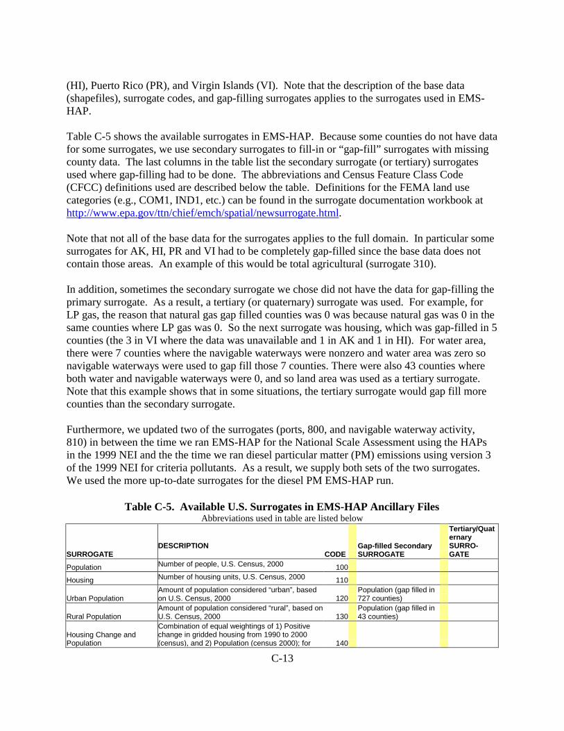
C-13
(HI), Puerto Rico (PR), and Virgin Islands (VI). Note that the description of the base data (shapefiles), surrogate codes, and gap-filling surrogates applies to the surrogates used in EMS-HAP. Table C-5 shows the available surrogates in EMS-HAP. Because some counties do not have data for some surrogates, we use secondary surrogates to fill-in or “gap-fill” surrogates with missing county data. The last columns in the table list the secondary surrogate (or tertiary) surrogates used where gap-filling had to be done. The abbreviations and Census Feature Class Code (CFCC) definitions used are described below the table. Definitions for the FEMA land use categories (e.g., COM1, IND1, etc.) can be found in the surrogate documentation workbook at http://www.epa.gov/ttn/chief/emch/spatial/newsurrogate.html. Note that not all of the base data for the surrogates applies to the full domain. In particular some surrogates for AK, HI, PR and VI had to be completely gap-filled since the base data does not contain those areas. An example of this would be total agricultural (surrogate 310). In addition, sometimes the secondary surrogate we chose did not have the data for gap-filling the primary surrogate. As a result, a tertiary (or quaternary) surrogate was used. For example, for LP gas, the reason that natural gas gap filled counties was 0 was because natural gas was 0 in the same counties where LP gas was 0. So the next surrogate was housing, which was gap-filled in 5 counties (the 3 in VI where the data was unavailable and 1 in AK and 1 in HI). For water area, there were 7 counties where the navigable waterways were nonzero and water area was zero so navigable waterways were used to gap fill those 7 counties. There were also 43 counties where both water and navigable waterways were 0, and so land area was used as a tertiary surrogate. Note that this example shows that in some situations, the tertiary surrogate would gap fill more counties than the secondary surrogate. Furthermore, we updated two of the surrogates (ports, 800, and navigable waterway activity, 810) in between the time we ran EMS-HAP for the National Scale Assessment using the HAPs in the 1999 NEI and the the time we ran diesel particular matter (PM) emissions using version 3 of the 1999 NEI for criteria pollutants. As a result, we supply both sets of the two surrogates. We used the more up-to-date surrogates for the diesel PM EMS-HAP run.
Table C-5. Available U.S. Surrogates in EMS-HAP Ancillary Files
Abbreviations used in table are listed below
SURROGATE
DESCRIPTION
CODE Gap-filled Secondary SURROGATE
Tertiary/Quaternary SURRO-GATE
Population Number of people, U.S. Census, 2000 100
Housing Number of housing units, U.S. Census, 2000 110
Urban Population Amount of population considered “urban”, based on U.S. Census, 2000 120
Population (gap filled in 727 counties)
Rural Population Amount of population considered “rural”, based on U.S. Census, 2000 130
Population (gap filled in 43 counties)
Housing Change and Population
Combination of equal weightings of 1) Positive change in gridded housing from 1990 to 2000 (census), and 2) Population (census 2000); for 140

C-14
Table C-5. Available U.S. Surrogates in EMS-HAP Ancillary Files Abbreviations used in table are listed below
SURROGATE
DESCRIPTION
CODE Gap-filled Secondary SURROGATE
Tertiary/Quaternary SURRO-GATE
AK, HI, PR, VI used population (year 2000)
Residential Heating - Natural Gas
Number of units with home heating as utility gas, from Census 2000. No data for VI, use housing surrogate. 150
Housing (gap filled in 25 counties)
Residential Heating - Wood
Number of units with home heating as wood from Census 2000. No data for VI, use housing surrogate. 160
Housing (gap filled in 88 counties)
Residential Heating - Distillate Oil
Number of units with home heating as fuel oil from Census 2000. No data for VI, use housing surrogate. 170
Housing (gap filled in 212 counties)
Residential Heating - Coal
Number of units with home heating as coal from Census 2000. No data for VI, use housing surrogate. 180
Housing (gap filled in 1883 counties)
Residential Heating - LP Gas
Number of units with home heating as bottled gas from Census 2000. No data for VI, use housing surrogate. 190
Residential Heating - Natural Gas (gap filled in 0 counties)
Housing (gap filled in 5 counties)
Urban Primary Road Miles
Road miles of urban primary roads (TIGER 2000, CFCC classes A11-A18, A21-A28 plus A63, overlayed with US Census 2000 urban areas). No data for VI, use total road miles. 200
Total Road Miles (gap filled in 946 counties)
Population (gap filled in 24 counties)
Rural Primary Road Miles
Road miles of rural primary roads (TIGER 2000, CFCC classes A11-A18, A21-A28 plus A63, overlayed with US Census 2000 rural areas). No data for VI, use total road miles. 210
Total Road Miles (gap filled in 251 counties)
Population (gap filled in 24 counties)
Urban Secondary Road Miles
Road miles of urban secondary roads (TIGER 2000, CFCC classes A31-A38 plus A63, overlayed with US Census 2000 urban areas) 220
Total Road Miles (gap filled in 984 counties)
Population (gap filled in 24 counties)
Rural Secondary Road Miles
Road miles of rural secondary roads (TIGER 2000, CFCC classes A31-A38 plus A63, overlayed with US Census 2000 rural areas)
230 Total Road Miles (gap filled in 103 counties)
Population (gap filled in 24 counties)
Total Road Miles
Sum of urban primary, rural primary, urban secondary and rural secondary (doesn’t include local roads) 240
Population (gap filled in 24 counties)
Urban Primary plus Rural Primary
No data for VI, use total road miles.
250 Total Road Miles (gap filled in 216 counties)
Population (gap filled in 24 counties)
3/4 Roadway Miles plus 1/4 population
Combination of population surrogate (Census 2000) and total road miles surrogates (Tiger 2000), weighted ¾ for roadway and ¼ for population 255
Total Railroad Miles
Sum of railroad miles of class 1, class 2&3, and unknown classified railroads from BTS/NTA Data from 2001 for conterminous U.S.; TIGER railroad data (2000) for AK/HI. No data for VI, use total road miles. 260
Total Road Miles (gap filled in 423 counties)
Population (gap filled in 20 counties)
Class 1 Railroad Miles
railroad miles of class 1 railroads from BTS/NTA Data from 2001 for conterminous U.S.; TIGER railroad data (2000) for AK/HI. No data for AK, HI,PR, VI. Use total railroad miles for AK, HI, PR. Use total road miles for VI.
270
Total Railroad Miles (gap filled in 558 counties)
Total Road Miles/ Population (gap filled in 423/20 counties)
Class 2 and 3 Railroad Miles
railroad miles of class 2&3 railroads from BTS/NTA Data from 2001 for conterminous U.S.; TIGER railroad data (2000) for AK/HI. No data for AK, HI, PR, VI. Use total railroad miles for AK, HI, 280
Total Railroad Miles (gap filled in 1258 counties)
Total Road Miles/ Population (gap filled in

C-15
Table C-5. Available U.S. Surrogates in EMS-HAP Ancillary Files Abbreviations used in table are listed below
SURROGATE
DESCRIPTION
CODE Gap-filled Secondary SURROGATE
Tertiary/Quaternary SURRO-GATE
PR. Use total road miles for VI. 423/20 counties)
Low Intensity Residential
Land area classified as low intensity residential from NLCD (1992 Landsat imagery). No data for VI, use RES1 surrogate. 300
Single Family Dwellings (RES1) (gap filled in 119 counties)
Total Agriculture
Sum of land area of the following NLCD (1992 Landsat imagery) classes: pasture/hay, grains, row crops, fallow land and orchards/vineyards. Nodata for AK, HI, PR, VI, use rural land area. 310
Rural Land Area (gap filled in 121 counties)
Land Area (gap filled in 7 counties)
Total Agriculture without Orchards/Vineyards
Sum of land area of the following NLCD (1992 Landsat imagery) classes: pasture/hay, grains, row crops and fallow land. No data for AK, HI, PR, VI, use rural land area. 311
Rural Land Area (gap filled in 122 counties)
Land Area (gap filled in 7 counties)
Orchards/Vineyards
Land area classified as orchards/vineyards from NLCD (1992 Landsat imagery). No data for AK, HI, PR, VI, use rural land area.
312 Total Agriculture (gap filled in 2886 counties)
Rural Land Area/ Land Area (gap filled in 121/7 counties)
Forest Land
Land area classified as forest from NLCD (1992 Landsat imagery). No data for AK, HI, PR, VI, userural land area. 320
Rural Land Area (gap filled in 175 counties)
Land Area (gap filled in 5 counties)
Strip Mines/Quarries
Land area classified as strip mines/quarries from NLCD(1992 Landsat imagery). No data for AK, HI, PR, VI (AK, HI use mines surrogate; PR, VI use rural land area)
330 Mines (gap filled in 408 counties)
Rural Land Area/ Land Area (gap filled in 590/13 counties)
Land Area All area not classified as open water from NLCD (1992 Landsat imagery) 340
Water
Areas classified as open water from NLCD (1992 Landsat imagery)
350
Navigable Waterway Miles (gap filled in 7 counties)
Land Area (gap filled in 43 counties)
Rural Land Area Areas not designated as an urbanized area or an urban cluster by Census 2000 400
Land (gap filled in 17 counties)
Commercial Land
Sum of FEMA building square footage in each 1990 census tract, from the following categories: COM1, COM2, COM3, COM4, COM5, COM6, COM7, COM8 and COM9 500
Industrial Land
Sum FEMA building square footage in each 1990 census tract, from the following categories: IND1, IND2, IND3, IND4, IND5 and IND6 505
Population (gap filled in 1 county)
Commercial plus Industrial
Sum of FEMA building square footage in each 1990 census tract, from all categories that make up commercial and industrial land surrogates 510
Commercial plus Institutional Land
Sum of FEMA building square footage in each 1990 census tract, from all categories that make up commercial land plus the following FEMA categories: RES5, RES6, EDU1, EDU2, and REL1 515
Commercial plust Industrial plus Institutional
Sum of FEMA building square footage in each 1990 census tract, from all categories that make up commercial land and industrial land plus the following FEMA categories: RES5, RES6, EDU1, EDU2, and REL1 520
Golf Courses plus Institutional plus Industrial plus Commercial
Combination surrogate made up of equal weightings of 1) number of golf courses from ESRIgolf course data, and 2) Institutional plus industrial plus commercial surrogate 525

C-16
Table C-5. Available U.S. Surrogates in EMS-HAP Ancillary Files Abbreviations used in table are listed below
SURROGATE
DESCRIPTION
CODE Gap-filled Secondary SURROGATE
Tertiary/Quaternary SURRO-GATE
Residential_High Density (RES3 + RES4 + RES5 + RES6)
Sum of Federal Emergency Management Agency (FEMA) building square footage in each 1990 census tract, from the following FEMA residential categories: RES3, RES4, RES5 and RES6. 530
Residential (RES1-4) + Commercial + Industrial + Institutional + Government
Sum of FEMA building square footage in each 1990 census tract, from all FEMA categories making up the commercial and industrial surrogates plus the following FEMA categories: RES1, RES2, RES3, RES4, EDU1, EDU2, REL1, GOV1, GOV2 535
Retail Trade (COM1) FEMA building square footage in each 1990 census tract, from retail trade (COM1) 540
Personal Repair (COM3) FEMA building square footage in each 1990 census tract, from personal repair (COM3) 545
Retail (COM1) (gap filled in 3 counties)
Retail Trade (COM1) plus Personal Repair (COM3)
Sum of FEMA building square footage in each 1990 census tract, from retail trade (COM1) and personal repair (COM3) 550
Professional/Technical (COM4) plus General Government (GOV1)
Sum of FEMA building square footage in each 1990 census tract, from Professional/Technical (COM4) and General Government (GOV1) 555
Hospital (COM6)
FEMA building square footage in each 1990 census tract, from hospitals (COM6)
560
Medical Office/Clinic (COM7) (gap filled in 512 counties)
Commercial Land (gap filled in 11 counties)
Medical Office/Clinic (COM7)
FEMA building square footage in each 1990 census tract, from Medical Office/Clinic (COM7)
565 Hospital (COM6) (gap filled in 2 counties)
Commercial Land (gap filled in 11 counties)
Heavy and High Tech Industrial (IND1 + IND5)
Sum FEMA building square footage in each 1990 census tract, from Heavy and High Tech Industrial (IND1 + IND5) 570
Industrial Land (gap filled in 18 counties)
Population (gap filled in 1 county)
Light and High Tech Industrial (IND2 + IND5)
Sum of FEMA building square footage in each 1990 census tract, from Light and High Tech Industrial (IND2 + IND5) 575
Industrial Land (gap filled in 11 counties)
Population (gap filled in 1 county)
Food, Drug, Chemical Industrial (IND3)
FEMA building square footage in each 1990 census tract, from Food, Drug, Chemical Industrial(IND3) 580
Industrial Land (gap filled in 119 counties)
Population (gap filled in 1 county)
Metals and Minerals Industrial (IND4)
FEMA building square footage in each 1990 census tract, from Metals and Minerals Industrial (IND4) 585
Industrial Land (gap filled in 226 counties)
Population (gap filled in 1 county)
Heavy Industrial (IND1)
FEMA building square footage in each 1990 census tract, from Heavy Industrial (IND1)
590 Industrial Land (gap filled in 19 counties)
Population (gap filled in 1 county)
Light Industrial (IND2)
FEMA building square footage in each 1990 census tract, from Light Industrial (IND2)
595 Industrial Land (gap filled in 11 counties)
Population (gap filled in 1 county)
Industrial plus Institutional plus Hospitals
Sum FEMA building square footage in each 1990 census tract, from all FEMA categories making up the industrial surrogate plus the following categories: RES5, RES6, EDU1, EDU2, and REL1 plus hospitals (COM6) 596
Gas Stations
Number of gas stations from Spatial Insights – business counts data base based on year 2000 data. No data for PR, VI, use commercial land. 600
Commercial Land (gap filled in 196 counties)
Refineries and Tank Farms
Number of refineries and tank farms from FEMA Database published 1999. No data for PR, VI, use industrial land. 650
Industrial Land (gap filled in 2697 counties)
Population (gap filled in 1 county)
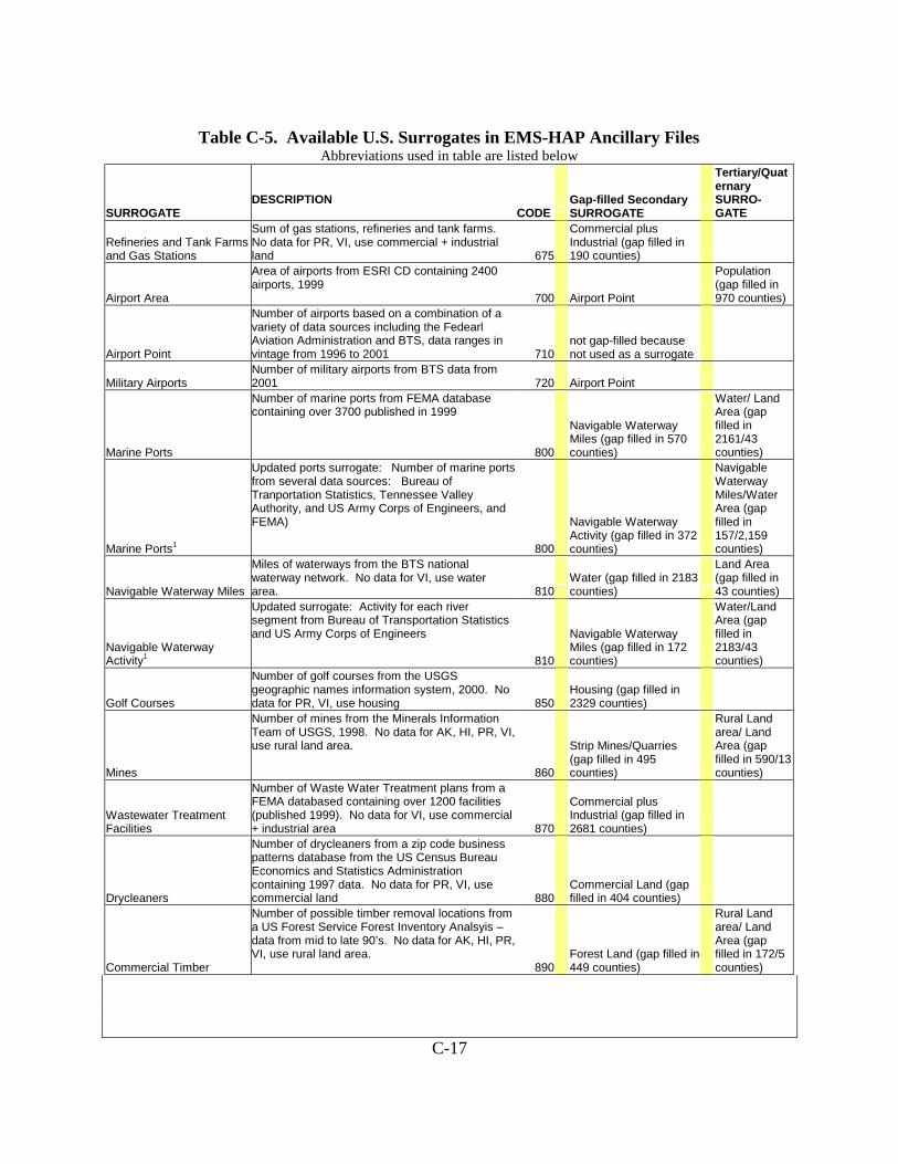
C-17
Table C-5. Available U.S. Surrogates in EMS-HAP Ancillary Files Abbreviations used in table are listed below
SURROGATE
DESCRIPTION
CODE Gap-filled Secondary SURROGATE
Tertiary/Quaternary SURRO-GATE
Refineries and Tank Farms and Gas Stations
Sum of gas stations, refineries and tank farms. No data for PR, VI, use commercial + industrial land 675
Commercial plus Industrial (gap filled in 190 counties)
Airport Area
Area of airports from ESRI CD containing 2400 airports, 1999
700 Airport Point
Population (gap filled in 970 counties)
Airport Point
Number of airports based on a combination of a variety of data sources including the Fedearl Aviation Administration and BTS, data ranges in vintage from 1996 to 2001 710
not gap-filled because not used as a surrogate
Military Airports Number of military airports from BTS data from 2001 720 Airport Point
Marine Ports
Number of marine ports from FEMA database containing over 3700 published in 1999
800
Navigable Waterway Miles (gap filled in 570 counties)
Water/ Land Area (gap filled in 2161/43 counties)
Marine Ports1
Updated ports surrogate: Number of marine ports from several data sources: Bureau of Tranportation Statistics, Tennessee Valley Authority, and US Army Corps of Engineers, and FEMA)
800
Navigable Waterway Activity (gap filled in 372 counties)
Navigable Waterway Miles/Water Area (gap filled in 157/2,159 counties)
Navigable Waterway Miles
Miles of waterways from the BTS national waterway network. No data for VI, use water area. 810
Water (gap filled in 2183 counties)
Land Area (gap filled in 43 counties)
Navigable Waterway Activity1
Updated surrogate: Activity for each river segment from Bureau of Transportation Statistics and US Army Corps of Engineers
810
Navigable Waterway Miles (gap filled in 172 counties)
Water/Land Area (gap filled in 2183/43 counties)
Golf Courses
Number of golf courses from the USGS geographic names information system, 2000. No data for PR, VI, use housing 850
Housing (gap filled in 2329 counties)
Mines
Number of mines from the Minerals Information Team of USGS, 1998. No data for AK, HI, PR, VI,use rural land area.
860
Strip Mines/Quarries (gap filled in 495 counties)
Rural Land area/ Land Area (gap filled in 590/13 counties)
Wastewater Treatment Facilities
Number of Waste Water Treatment plans from a FEMA databased containing over 1200 facilities (published 1999). No data for VI, use commercial + industrial area 870
Commercial plus Industrial (gap filled in 2681 counties)
Drycleaners
Number of drycleaners from a zip code business patterns database from the US Census Bureau Economics and Statistics Administration containing 1997 data. No data for PR, VI, use commercial land 880
Commercial Land (gap filled in 404 counties)
Commercial Timber
Number of possible timber removal locations from a US Forest Service Forest Inventory Analsyis – data from mid to late 90’s. No data for AK, HI, PR,VI, use rural land area.
890 Forest Land (gap filled in 449 counties)
Rural Land area/ Land Area (gap filled in 172/5 counties)

C-18
Abbreviations Used in Above Table C-5: CFCC: census feature class code. Used to identify the most noticeable characteristic of a feature. CFCC descriptions: A11 Primary road with limited access or interstate highway, unseparated A12 Primary road with limited access or interstate highway, unseparated, in tunnel A13 Primary road with limited access or interstate highway, unseparated, underpassing A14 Primary road with limited access or interstate highway, unseparated, with rail line in center A15 Primary road with limited access or interstate highway, separated A16 Primary road with limited access or interstate highway, separated, in tunnel A17 Primary road with limited access or interstate highway, separated, underpassing A18 Primary road with limited access or interstate highway, separated, with rail line in center A21 Primary road without limited access, US highways, unseparated A22 Primary road without limited access, US highways, unseparated, in tunnel A23 Primary road without limited access, US highways, unseparated, underpassing A24 Primary road without limited access, US highways, unseparated, with rail line in center A25 Primary road without limited access, US highways, separated A26 Primary road without limited access, US highways, separated, in tunnel A27 Primary road without limited access, US highways, separated, underpassing A28 Primary road without limited access, US highways, separated, with rail line in center A63 Access ramp, the portion of a road that forms a cloverleaf or limited access interchange A31 Secondary and connecting road, state highways, unseparated A32 Secondary and connecting road, state highways, unseparated, in tunnel A33 Secondary and connecting road, state highways, unseparated, underpassing A34 Secondary and connecting road, state highways, unseparated, with rail line in center A35 Secondary and connecting road, state highways, separated A36 Secondary and connecting road, state highways, separated, in tunnel A37 Secondary and connecting road, state and county highways, separated, underpassing A38 Secondary and connecting road, state and county highways, separated, with rail line in center AK: Alaska; HI: Hawaii; VI: Virgin Islands; PR: Puerto Rico BTS: Bureau of Transportation Statistics BTS/NTA: Burea of Transportation Statistics/National Transportation Atlas NLCD: National Land Cover Data FEMA: Federal Emergency Management Agency USGS: U.S. Geological Survey Notes: 1. Marine ports and Navigable Waterway activity were modified after the 1999 NEI emissions were processed through EMS-HAP. The modified marine ports and navigable waterway activity surrogates were used for the 1999 Diesel PM inventory. Ports were gap filled past the quaternary surrogate with land area in 43 counties.
Tables C-6 through C-8 show how the available surrogates were used with the 1999 NATA non-point, nonroad mobile, and onroad mobile categories, respectively.

C-19
Table C- 6 Surrogates Assigned to 1999 NEI Non-point Source Categories for Spatial Allocation Surrogate Name
(and code) Emissions Inventory Categories (and SCC codes) Population (100) Consumer and Commercial Products Usage: all products and types (2460000000), Consumer and Commercial Products Usage: Personal Care Products, all
types (2460100000), Consumer and Commercial Products Usage: Personal Care Products - Hair Care (2460110000), Consumer and Commercial Products Usage: Personal Care Products - Nail Care (2460150000), Consumer and Commercial Products Usage: Personal Care Products - Health Use (2460180000), Consumer and Commercial Products Usage: Personal Care Products - Miscellaneous (2460190000), Consumer and Commercial Products Usage: Household Products, all types (2460200000), Consumer and Commercial Products Usage: Household Products - Laundry (2460220000), Consumer and Commercial Products Usage: Automotive Aftermarket Products (2460400000), Consumer and Commercial Products Usage: Coating and Related Products (2460500000), Consumer and Commercial Products Usage: Adhesives and Sealants, all types (2460600000), Consumer and Commercial Products Usage: Adhesive and Sealants - Wallpapering (2460610000), Consumer and Commercial Products Usage: FIFRA-Regulated Products (2460800000), Consumer and Commercial Products Usage: Miscellaneous (2460900000), Consumer Products Usage - All products/processes, all solvent types (2465000000), Consumer Products Usage -All products/processes using Ethylbenzene (2465000185), Consumer Products Usage - All products/processes using Methanol (2465000260), Consumer Products Usage - All products/processes using Methyl Isobutyl Ketone (2465000285), Consumer Products Usage - All products/processes using p-Dichlorobenzene (2465000340), Consumer Products Usage - All products/processes using Perchloroethylene (2465000345), Consumer Products Usage - All products/processes using Special Naphthas (2465000370), Consumer Products Usage - Personal Care Products (2465100000), Consumer Products Usage - Household Products (2465200000), Consumer Products Usage - Automotive Aftermarket Products (2465400000), Consumer Products Usage - Adhesives and Sealants (2465600000), Consumer Products Usage - Pesticide Application (2465800000), Consumer Products Usage - Miscellaneous Products, nec (2465900000), Human Perspiration (2810010000), Swimming Pools (2862000000)
Housing Change and Population (140)
Construction - General Building (2311010000), Construction - Roads (2311030000), Asphalt Paving: Cutback and Emulsified (2461020000), Asphalt Paving: Cutback (2461021000), Asphalt Paving: Emulsified (2461022000), Commercial Asphalt Roofing (2461023000), Open Burning - Land Clearing Debris (2610000500)
Residential Heating - Natural Gas (150)
Residential Heating: Natural Gas - All types (2104006000), Residential Heating: Natural Gas from Furnace (2104006010)
Residential Heating - Wood (160)
Residential Heating: Wood/Wood Residue (2104008000), Fireplaces (2104008001), Fireplaces: Inserts; non-EPA certified (2104008002), Fireplaces: Inserts; non catalytic, EPA certified (2104008003), Fireplaces: Inserts; catalytic, EPA certified (2104008004), Residential Wood Heating: Woodstoves - conventional (2104008010), Residential Wood Heating: Catalytic Woodstoves - General (2104008030), Residential Heating: Non-catalytic Woodstoves - General (2104008050), Residential Heating: Non-catalytic Woodstoves - Conventional (2104008051), Residential Heating: Non-catalytic Woodstoves - Pellet-fired (2104008053)
Residential Heating - Distillate Oil (170)
Residential Heating: Distillate Oil (2104004000)
Residential Heating - Coal (180)
Residential Heating: Anthracite Coal (2104001000), Residential Heating: Bituminous and Lignite Coal (2104002000)
Residential Heating - LP Gas (190)
Residential Heating: Liquified Petroleum Gas (2104007000)
Total Road Miles (240) Surface Coatings: Traffic Markings, all coating types (2401008000), Surface Coatings: Traffic Markings using Acetone (2401008030), Surface Coatings: Traffic Markings using Glycol Ethers (2401008235), Surface Coatings: Traffic Markings using Methyl Ethyl Ketone (2401008275), Surface Coatings: Traffic Markings using Methyl Isobutyl Ketone (2401008285), Surface Coatings: Traffic Markings using Special Naphthas (2401008370), Surface Coatings: Traffic Markings, NEC (2401008999), Motor Vehicle Fires (2810050000)
Urban Primary plus Rural Primary (250)
Petroleum Prod Distribution: All Products - All Transport Types (2505000000), Gasoline Distribution: Gasoline - All Transport Types (2505000120), Gasoline Distribution: Gasoline - Truck Transport (2505030120), Gasoline Distribution: Kerosene - Truck Transport (2505030180), Transit Losses from Gasoline Transportation and Marketing (Tank Cars & Trucks) (40600162)
Total Railroad Miles (260)
Petroleum Prod Distribution: All Products - Rail Tank Car (2505010000)

C-20
Table C- 6 Surrogates Assigned to 1999 NEI Non-point Source Categories for Spatial Allocation Surrogate Name
(and code) Emissions Inventory Categories (and SCC codes) Low Intensity Residential (300)
Open Burning - Yard Waste - Leaf Species Unspecified (2610000100), Open Burning - Yard Waste: Weed Species Unspecified (2610000300), Open Burning - Yard Waste - Brush Species Unspecified (2610000400), Open Burning - Residential, Household Waste (2610030000), Landfills - All types (2620000000), Municipal Landfills (2620030000), Waste Disposal, Treatment, and Recovery: all types (2640000000), Charcoal Grilling (2810025000), Human Cremation (2810060100), Animal Cremation (2810060200), Lamp Breakage (2861000000), Asphalt Concrete Manufacturing - Rotary Dryer at a Conventional Plant (30500201)
Total Agriculture (310) Commercial Pesticide Application - agricultural pesticides, total (2461850000), Commercial Pesticide Application - agricultural herbicides for Corn (2461850001) Total Agriculture without Orchards/Vineyards (311)
Commercial Pesticide Application - agricultural herbicides for Soy Beans (2461850005), Commercial Pesticide Application - agricultural herbicides for Hay and Grains (2461850006), Commercial Pesticide Application - agricultural herbicides for Other Pesticide (2461850051), Agricultural Crop Tilling (2801000003), Agricultural Field Burning - all crops (2801500000), Agricultural Field Burning: Field Crop Unspecified (2801500100), Agricultural Field Burning: whole field set on fire, Barley (2801500130), Agricultural Field Burning: Field Crop is Grasses (2801500170), Agricultural Field Burning: whole field set on fire, Wheat (2801500261), Agricultural Propaing - tractor-pulled burners to stubble only (2801501000), Agricultural Stack Burning - straw stacks moved from field for burning (2801502000), Country Grain Elevators (2801600000), Agricultural Production - Livestock (2805000000), Cotton Ginning (30200410), Grain Elevators: Country and Terminal (30200512)
Orchards/Vineyards (312)
Agricultural Field Burning - unspecified orchard crop (2801500300), Agricultural Field Burning - apple orchard crop (2801500320), Agricultural Field Burning - cherry orchard crop (2801500350), Agricultural Field Burning: Orchard Crop is Citrus (2801500360), Agricultural Field Burning - peach orchard crop (2801500410), Agricultural Field Burning - pear orchard crop (2801500420), Agricultural Field Burning - prune orchard crop (2801500430), Agricultural Field Burning - walnut orchard crop (2801500440), Agricultural Field Burning - hazelnut orchard crop (2801500450), Agricultural Field Burning - unspecified vine crop (2801500500), Orchard Heaters (2801520000), Orchard Heaters - diesel fuel (2801520004)
Forest Land (320) Soil/Agricultural (2701420000), Open Burning - Forest and Wildfires (2810001000), Logging/Slash Burning (2810005000), Open Burning - Prescribed Burning (2810015000), Prescribed Rangeland Burning (2810020000)
Strip Mines/Quarries (330)
Mining and Quarrying of Sand and Gravel (2325030000)
Rural Land Area (400) Open Burning - All types (not specified) (2610000000), Geyser/Geothermal (2730050000), Wind Erosion (2730100000) Industrial Land (505) Industrial Boilers: Distillate Oil (10200501), Industrial Boilers: Wood/Bark Waste, Bark-fired Boiler (10200901), Industrial Boilers: Waste Oil (10201302), Electric
Utility Combustion: Natural Gas (2101006000), Industrial Boilers: Bituminous/Subbituminous Coal (2102002000), Industrial Boilers and IC Engines: Distillate Oil (2102004000), Industrial Boilers: Residual Oil (2102005000), Industrial Boilers and IC Engines: Natural Gas (2102006000), Industrial Boilers: Natural Gas (2102006001), Industrial IC Engines: Natural Gas (2102006002), Industrial Boilers - Liquified Petroleum Gas (2102007000), Industrial Boilers: Wood Combustion (2102008000), Industrial Boilers: Kerosene (2102011000), Other Industral Processes (2399000000), Surface Coatings: Miscellaneous Metals Manufacturing (2401090000), Surface Coatings: Miscellaneous Manufacturing, not elsewhere classified (2401090999), Surface Coatings: Industrial Maintenance, all coating types (2401100000), Surface Coatings: Industrial Maintenance, nec (2401100999), Scrap and Waste Materials Crushing (2650000001), Open Burning - Scrap Tires (2830000000), Electrical Equipment - Light Bulb Manufacture (31301001), Fluorescent Lamp Recycling (31301200), Boat Manufacturing, General (31401501), Boat Manufacturing - Gel Coat Application (31401511), Boat Manufacturing - Resin Spraying (31401515), Boat Manufacturing - Resin Brushing (31401516), Natural Gas Storage in Pressure Tanks (39092050), Site Remediation (50490004)
Commercial plus Industrial (510)
Degreasing - All Industries, processes, and solvents (2415000000), Degreasing - All Industries: All Processes using Perchloroethylene (2415000350), Degreasing - All Industries: All Processes using Trichloroethylene (2415000385), Degreasing - All Industries: Open Top, all solvent types (2415100000), Degreasing - All Industries: Open Top using Perchloroethylene (2415100350), Degreasing - All Industries: Open Top using Trichloroethylene (2415100385), Degreasing - All Industries: Cold Cleaning, all solvent types (2415300000), Degreasing - All Industries: Cold Cleaning using Perchloroethylene (2415300350), Degreasing - All Industries: Cold Cleaning using Trichloroethylene (2415300385), Graphic Arts: All types and solvents (2425000000), Graphic Arts: All Processes using Special Naphthas (2425000370), Graphic Arts: Lithography using Butyl Acetate (2425010055), Graphic Arts: Lithography using Special Naphthas (2425010370), Graphic Arts: Flexography using All Solvent Types (2425040000), Graphic Arts: Flexography using Special Naphthas (2425040370), Solvent Use on Rubber/Plastics (2430000000), Miscellaneous Industrial Solvent Usage (2440000000), Industrial Adhesive Application (2440020000), Petroleum and
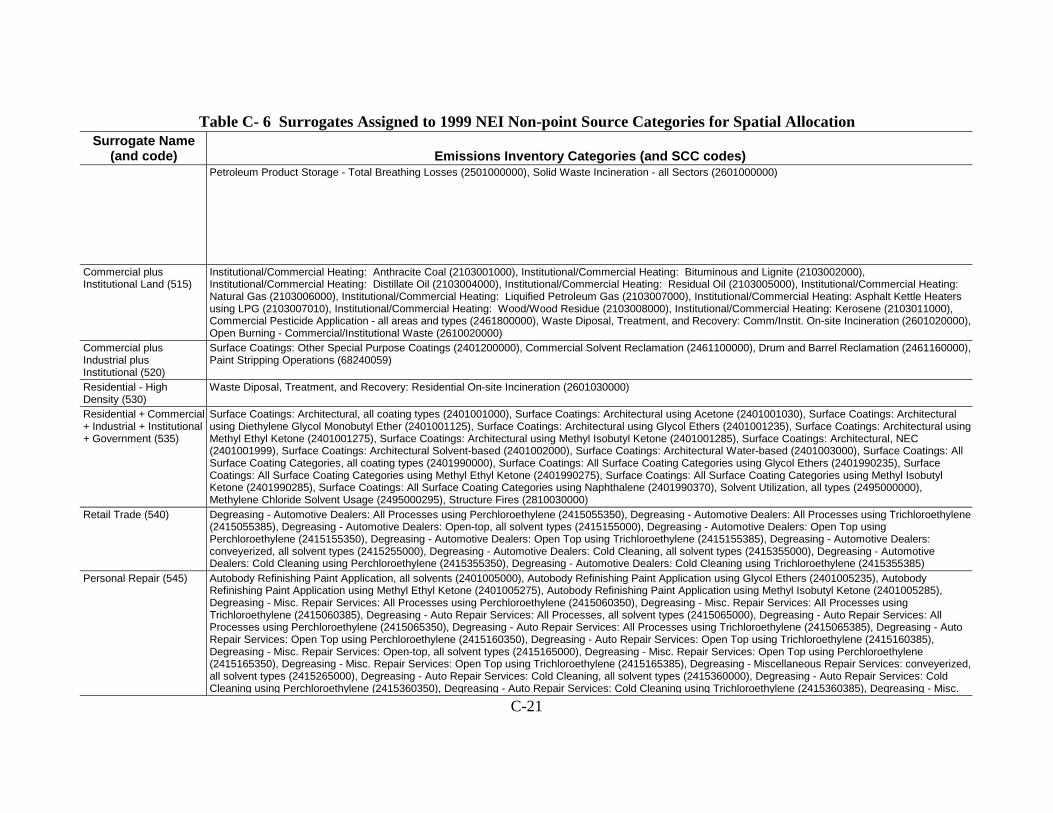
C-21
Table C- 6 Surrogates Assigned to 1999 NEI Non-point Source Categories for Spatial Allocation Surrogate Name
(and code) Emissions Inventory Categories (and SCC codes) Petroleum Product Storage - Total Breathing Losses (2501000000), Solid Waste Incineration - all Sectors (2601000000)
Commercial plus Institutional Land (515)
Institutional/Commercial Heating: Anthracite Coal (2103001000), Institutional/Commercial Heating: Bituminous and Lignite (2103002000), Institutional/Commercial Heating: Distillate Oil (2103004000), Institutional/Commercial Heating: Residual Oil (2103005000), Institutional/Commercial Heating: Natural Gas (2103006000), Institutional/Commercial Heating: Liquified Petroleum Gas (2103007000), Institutional/Commercial Heating: Asphalt Kettle Heaters using LPG (2103007010), Institutional/Commercial Heating: Wood/Wood Residue (2103008000), Institutional/Commercial Heating: Kerosene (2103011000), Commercial Pesticide Application - all areas and types (2461800000), Waste Diposal, Treatment, and Recovery: Comm/Instit. On-site Incineration (2601020000), Open Burning - Commercial/Institutional Waste (2610020000)
Commercial plus Industrial plus Institutional (520)
Surface Coatings: Other Special Purpose Coatings (2401200000), Commercial Solvent Reclamation (2461100000), Drum and Barrel Reclamation (2461160000), Paint Stripping Operations (68240059)
Residential - High Density (530)
Waste Diposal, Treatment, and Recovery: Residential On-site Incineration (2601030000)
Residential + Commercial + Industrial + Institutional + Government (535)
Surface Coatings: Architectural, all coating types (2401001000), Surface Coatings: Architectural using Acetone (2401001030), Surface Coatings: Architectural using Diethylene Glycol Monobutyl Ether (2401001125), Surface Coatings: Architectural using Glycol Ethers (2401001235), Surface Coatings: Architectural using Methyl Ethyl Ketone (2401001275), Surface Coatings: Architectural using Methyl Isobutyl Ketone (2401001285), Surface Coatings: Architectural, NEC (2401001999), Surface Coatings: Architectural Solvent-based (2401002000), Surface Coatings: Architectural Water-based (2401003000), Surface Coatings: All Surface Coating Categories, all coating types (2401990000), Surface Coatings: All Surface Coating Categories using Glycol Ethers (2401990235), Surface Coatings: All Surface Coating Categories using Methyl Ethyl Ketone (2401990275), Surface Coatings: All Surface Coating Categories using Methyl Isobutyl Ketone (2401990285), Surface Coatings: All Surface Coating Categories using Naphthalene (2401990370), Solvent Utilization, all types (2495000000), Methylene Chloride Solvent Usage (2495000295), Structure Fires (2810030000)
Retail Trade (540) Degreasing - Automotive Dealers: All Processes using Perchloroethylene (2415055350), Degreasing - Automotive Dealers: All Processes using Trichloroethylene (2415055385), Degreasing - Automotive Dealers: Open-top, all solvent types (2415155000), Degreasing - Automotive Dealers: Open Top using Perchloroethylene (2415155350), Degreasing - Automotive Dealers: Open Top using Trichloroethylene (2415155385), Degreasing - Automotive Dealers: conveyerized, all solvent types (2415255000), Degreasing - Automotive Dealers: Cold Cleaning, all solvent types (2415355000), Degreasing - Automotive Dealers: Cold Cleaning using Perchloroethylene (2415355350), Degreasing - Automotive Dealers: Cold Cleaning using Trichloroethylene (2415355385)
Personal Repair (545) Autobody Refinishing Paint Application, all solvents (2401005000), Autobody Refinishing Paint Application using Glycol Ethers (2401005235), Autobody Refinishing Paint Application using Methyl Ethyl Ketone (2401005275), Autobody Refinishing Paint Application using Methyl Isobutyl Ketone (2401005285), Degreasing - Misc. Repair Services: All Processes using Perchloroethylene (2415060350), Degreasing - Misc. Repair Services: All Processes using Trichloroethylene (2415060385), Degreasing - Auto Repair Services: All Processes, all solvent types (2415065000), Degreasing - Auto Repair Services: All Processes using Perchloroethylene (2415065350), Degreasing - Auto Repair Services: All Processes using Trichloroethylene (2415065385), Degreasing - Auto Repair Services: Open Top using Perchloroethylene (2415160350), Degreasing - Auto Repair Services: Open Top using Trichloroethylene (2415160385), Degreasing - Misc. Repair Services: Open-top, all solvent types (2415165000), Degreasing - Misc. Repair Services: Open Top using Perchloroethylene (2415165350), Degreasing - Misc. Repair Services: Open Top using Trichloroethylene (2415165385), Degreasing - Miscellaneous Repair Services: conveyerized, all solvent types (2415265000), Degreasing - Auto Repair Services: Cold Cleaning, all solvent types (2415360000), Degreasing - Auto Repair Services: Cold Cleaning using Perchloroethylene (2415360350), Degreasing - Auto Repair Services: Cold Cleaning using Trichloroethylene (2415360385), Degreasing - Misc.

C-22
Table C- 6 Surrogates Assigned to 1999 NEI Non-point Source Categories for Spatial Allocation Surrogate Name
(and code) Emissions Inventory Categories (and SCC codes) Repair Services: Cold Cleaning, all solvent types (2415365000), Degreasing - Misc. Repair Services: Cold Cleaning using Perchloroethylene (2415365350), Degreasing - Misc. Repair Services: Cold Cleaning using Trichloroethylene (2415365385), Automotive Repair Shops: Auto Top and Body Repair (2840010000)
Professional/Technical plus General Government (555)
Degreasing - Transportation Maint. Fac.: All Processes using Perchloroethylene (2415050350), Degreasing - Transportation Maint. Fac.: All Processes using Trichloroethylene (2415050385), Degreasing - Transportation Maint. Fac.: Open-top, all solvent types (2415150000), Degreasing - Transportation Maint. Fac.: Open Top using Perchloroethylene (2415150350), Degreasing - Transportation Maint. Fac.: Open Top using Trichloroethylene (2415150385), Degreasing - Transport. Mainten. Facilities: conveyerized, all solvent types (2415250000), Degreasing - Transportation Maint. Fac: Cold Cleaning, all types (2415350000), Degreasing - Transportation Maint. Fac.: Cold Cleaning using Perchloroethylene (2415350350), Degreasing - Transportation Maint. Fac.: Cold Cleaning using Trichloroethylene (2415350385)
Hospital (560) Hospital Sterilizers (2850000010), Medical Waste Incineration (2850000030), Hospital Laboratory (fugitive) (31502088) Medical Office/Clinic (565)
Dental Preparation and Use (31502500), General Laboratory Activities (31503001)
Heavy and High Tech Industrial (570)
Cement Manufacturing via Wet Process (30500799)
Light and High Tech Industrial (575)
Surface Coatings: Electronic and Other Electrical, all coating types (2401065000), Surface Coatings: Electronic and Other Electrical using Glycol Ethers (2401065235), Surface Coatings: Electronic and Other Electrical using Methyl Isobutyl Ketone (2401065285), Surface Coatings: Electronic and Other Electrical using Special Naphthas (2401065370), Degreasing - Electronic and Other Elec.: All Processes, all solvent types (2415030000), Degreasing - Electronic and Other Elec.: All Processes using Perchloroethylene (2415030350), Degreasing - Electronic and Other Elec.: All Processes using Trichloroethylene (2415030385), Degreasing - Electronic and Other Elec.: Open-top, all solvent types (2415130000), Degreasing - Electronic and Other Elec.: Open Top using Perchloroethylene (2415130350), Degreasing - Electronic and Other Elec.: Open Top using Trichloroethylene (2415130385), Degreasing - Electronic and Other Elec.: conveyerized, all solvent types (2415230000), Degreasing - Electronic and Other Elec.: Cold Cleaning, all types (2415330000), Degreasing - Electronic and Other Elec.: Cold Cleaning using Perchloroethylene (2415330350), Degreasing - Electronic and Other Elec.: Cold Cleaning using Trichlorethylene (2415330385), Fiberglass Resin Products - Gel Coat: Roll On (30800721), Fiberglass Resin Products - General: Roll On (30800723), Fiberglass Resin Products - General: Spray On (30800724), Flexible Polyurethane Foam Production (30801005)
Food, Drug, Chemical Industrial (580)
Chemical Manufacturing - All Types and Processes (2301000000), Industrial Inorganic Chemical Manufacturing, all processes (2301010000), Industrial Inorganic Chemical Manufacturing, Sulfur Recovery (2301010010), Synthetic Fibers Manufacturing (2301020000), Food and Kindred Products Manufacturing, all processes (2302000000), Commercial Charbroiling (2302002000), Miscellaneous Food Manufacturing (2302080000), Asphalt Roofing Materials Manufacturing (2306010000), Mercury-Cell Chloralkali Production (30100802), Flexible Polyurethane Foam Fabrication (30101880), Miscellaneous Organic Chemical Processes (30199999), Food and Agriculture - Grain Millings, Wet Corn Milling (30200756)
Metals and Minerals Industrial (585)
Steel Pickling HCl Process (2303000000), Secondary Metals Production (2304000000), Oil and Natural Gas Production - all fuel types (2310000000), Oil and Natural Gas Production - Crude Petroleum (2310010000), Oil and Natural Gas Production - Natural Gas (2310020000), Oil and Natural Gas Production - Natural Gas Liquids (2310030000), Degreasing - Primary Metal Industries: All Processes using Perchloroethylene (2415010350), Degreasing - Primary Metal Industries: All Processes using Trichloroethylene (2415010385), Degreasing - Primary Metal Industries: Open-top, all solvent types (2415110000), Degreasing - Primary Metal Industries: Open Top using Perchloroethylene (2415110350), Degreasing - Primary Metal Industries: Open Top using Trichloroethylene (2415110385), Degreasing - Primary Metal Industries: conveyerized, all solvent types (2415210000), Degreasing - Primary Metal Industries: Cold Cleaning, all solvent types

C-23
Table C- 6 Surrogates Assigned to 1999 NEI Non-point Source Categories for Spatial Allocation Surrogate Name
(and code) Emissions Inventory Categories (and SCC codes) (2415310000), Degreasing - Primary Metal Industries: Cold Cleaning using Perchloroethylene (2415310350), Degreasing - Primary Metal Industries: Cold Cleaning using Trichloroethylene (2415310385), Fabricated Metal Products - General Processes (30900199), Fabricated Metal Products - Electroplating Operations (30901006), Fabricated Metal Products - Porcelain Enamel/Ceramic Glaze Spraying (30906001), Natural Gas Transmissions and Storage (31000299)
Heavy Industrial (590) Refractories Manufacturing (2305000000), Concrete, Gypsum, and Plaster Products Manufacturing (2305070000), Cut Stone and Stone Products Manufacturing (2305080000), Wood Products Manufacturing, all processes (2307000000), Fabricated Metals Manufacturing, all processes (2309000000), Hard Chromium Electroplating (2309100010), Decorative Chromium Electroplating (2309100030), Chromic Acid Anodizing (2309100050), Machinery Manufacturing, all processes (2312000000), Surface Coatings: Textiles (2401010000), Surface Coatings: Factory-finished Wood, all coating types (2401015000), Surface Coatings: Factory Finished Wood using Glycol Ethers (2401015235), Surface Coatings: Factory Finished Wood using Methyl Isobutyl Ketone (2401015285), Surface Coatings: Factory Finished Wood using Special Naphthas (2401015370), Surface Coatings: Paper, all coating types (2401030000), Surface Coatings: Paper using Glycol Ethers (2401030235), Surface Coatings: Paper using Methyl Isobutyl Ketone (2401030285), Surface Coatings: Paper using Special Naphthas (2401030370), Surface Coatings: Metal Cans (2401040000), Surface Coatings: Metal Coils (2401045000), Surface Coatings: Miscellaneous Finished Parts (2401050000), Surface Coatings: Machinery and Equipment, all coating types (2401055000), Surface Coatings: Machinery and Equipment using Glycol Ethers (2401055235), Surface Coatings: Machinery and Equipment using Methyl Isobutyl Ketone (2401055285), Surface Coatings: Machinery and Equipment using Special Naphthas (2401055370), Surface Coatings: Motor Vehicles (2401070000), Surface Coatings: Motor Vehicles using Glycol Ethers (2401070235), Surface Coatings: Motor Vehicles using Methyl Isobutyl Ketone (2401070285), Surface Coatings: Motor Vehicles using Special Naphthas (2401070370), Surface Coatings: Aircrafts, all coating types (2401075000), Surface Coatings: Aircrafts using Glycol Ethers (2401075235), Surface Coatings: Aircrafts using Methyl Isobutyl Ketone (2401075285), Surface Coatings: Aircrafts using Special Naphthas (2401075370), Surface Coatings: Marine, all coating types (2401080000), Surface Coatings: Marine using Glycol Ethers (2401080235), Surface Coatings: Marine using Methyl Isobutyl Ketone (2401080285), Surface Coatings: Marine using Special Naphthas (2401080370), Surface Coatings: Railroads using Glycol Ethers (2401085235), Surface Coatings: Railroads using Methyl Isobutyl Ketone (2401085285), Surface Coatings: Railroads using Special Naphthas (2401085370), Degreasing - Fabricated Metal Products: All Processes using Perchloroethylene (2415020350), Degreasing - Fabricated Metal Products: All Processes using Trichloroethylene (2415020385), Degreasing - Industrial Machinery & Equip: All Proc. using Perchloroethylene (2415025350), Degreasing - Industrial Machinery & Equip: All Proc. using Trichloroethylene (2415025385), Degreasing - Transportation Equip. Man.: All Processes using Perchloroethylene (2415035350), Degreasing - Transportation Equip. Man.: All Processes using Trichloroethylene (2415035385), Degreasing - Fabricated Metal Products: Open-top, all solvent types (2415120000), Degreasing - Fabricated Metal Products: Open Top using Perchloroethylene (2415120350), Degreasing - Fabricated Metal Products: Open Top using Trichloroethylene (2415120385), Degreasing - Industrial Machinery & Equip: Open-top, all solvent types (2415125000), Degreasing - Industrial Machinery & Equip: Open Top using Perchloroethylene (2415125350), Degreasing - Industrial Machinery & Equip: Open Top using Trichloroethyl (2415125385), Degreasing - Transportation Equip. Man.: Open-top, all solvent types (2415135000), Degreasing - Transportation Equip. Man.: Open Top using Perchloroethylene (2415135350), Degreasing - Transportation Equip. Man.: Open Top using Trichloroethylene (2415135385), Degreasing - Fabricated Metal Products: conveyerized, all solvent types (2415220000), Degreasing - Indust. Machinery & Equipment: conveyerized, all solvent types (2415225000), Degreasing - Transportation Equipment: conveyerized, all solvent types (2415235000), Degreasing - Fabricated Metal Products: Cold Cleaning, all solvent types (2415320000), Degreasing - Fabricated Metal Products: Cold Cleaning using Perchloroethylene (2415320350), Degreasing - Fabricated Metal Products: Cold Cleaning using Trichlorethylene (2415320385), Degreasing - Industrial Machinery & Equip: Cold Clean., all solvent types (2415325000), Degreasing - Industrial Machinery & Equip: Cold Clean. using Perchloroethylene (2415325350), Degreasing - Industrial Machinery & Equip: Cold Clean. using Trichlorethylene (2415325385), Degreasing - Transportation Equip. Man.: Cold Cleaning, all solvent types (2415335000), Degreasing - Transportation Equip. Man.: Cold Cleaning using Perchloroethylene (2415335350), Degreasing - Transportation Equip. Man.: Cold Cleaning using Trichloroethylene (2415335385), Textile Products Manufacturing, Miscellaneous (33000198), Surface Coatings: Large Ships (40202301)

C-24
Table C- 6 Surrogates Assigned to 1999 NEI Non-point Source Categories for Spatial Allocation Surrogate Name
(and code) Emissions Inventory Categories (and SCC codes) Light Industrial (595) Rubber/Plastics Manufacturing, all processes (2308000000), Surface Coatings: Wood Furniture, all coating types (2401020000), Surface Coatings: Wood
Furniture using Glycol Ethers (2401020235), Surface Coatings: Wood Furniture using Methyl Isobutyl Ketone (2401020285), Surface Coatings: Wood Furniture using Special Naphthas (2401020370), Surface Coatings: Metal Furniture, all coating types (2401025000), Surface Coatings: Metal Furniture using Glycol Ethers (2401025235), Surface Coatings: Metal Furniture using Methyl Isobutyl Ketone (2401025285), Surface Coatings: Metal Furniture using Special Naphthas (2401025370), Surface Coatings: Plastic Products, all coating types (2401035000), Surface Coatings: Plastic Products using Glycol Ethers (2401035235), Surface Coatings: Plastic Products using Methyl Isobutyl Ketone (2401035285), Surface Coatings: Plastic Products using Special Naphthas (2401035370), Surface Coatings: Large Appliances (2401060000), Degreasing - Furniture and Fixtures: All Processes using Perchloroethylene (2415005350), Degreasing - Furniture and Fixtures: All Processes using Trichloroethylene (2415005385), Degreasing - Instruments & Rel. Product: All Processes using Perchloroethylene (2415040350), Degreasing - Instruments & Rel. Product: All Processes using Trichloroethylene (2415040385), Degreasing - Misc. Manufacturing: All Processes, all solvent types (2415045000), Degreasing - Misc. Manufacturing: All Processes using Perchloroethylene (2415045350), Degreasing - Misc. Manufacturing: All Processes using Trichloroethylene (2415045385), Degreasing - Furniture and Fixtures: Open-top, all solvent types (2415105000), Degreasing - Furniture and Fixtures: Open Top using Perchloroethylene (2415105350), Degreasing - Furniture and Fixtures: Open Top using Trichloroethylene (2415105385), Degreasing - Instruments & Rel. Product: Open-top, all solvent types (2415140000), Degreasing - Instruments & Rel. Product: Open Top using Perchloroethylene (2415140350), Degreasing - Instruments & Rel. Product: Open Top using Trichloroethylene (2415140385), Degreasing - Misc. Manufacturing: Open-top, all solvent types (2415145000), Degreasing - Misc. Manufacturing: Open Top using Perchloroethylene (2415145350), Degreasing - Misc. Manufacturing: Open Top using Trichloroethylene (2415145385), Degreasing - Furniture & Fixtures: conveyerized, all solvent types (2415205000), Degreasing - Instruments & Related Products: conveyerized, all solvent types (2415240000), Degreasing - Misc. Manufacturing: conveyerized, all solvent types (2415245000), Degreasing - Furniture and Fixtures: Cold Cleaning, all solvent types (2415305000), Degreasing - Furniture and Fixtures: Cold Cleaning using Perchloroethylene (2415305350), Degreasing - Furniture and Fixtures: Cold Cleaning using Trichlorethylene (2415305385), Degreasing - Instruments & Rel. Product: Cold Cleaning, all solvent types (2415340000), Degreasing - Instruments & Rel. Product: Cold Cleaning using Perchloroethylene (2415340350), Degreasing - Instruments & Rel. Product: Cold Cleaning using Trichloroethylene (2415340385), Degreasing - Misc. Manufacturing: Cold Cleaning, all types (2415345000), Degreasing - Misc. Manufacturing: Cold Cleaning using Perchloroethylene (2415345350), Degreasing - Misc. Manufacturing: Cold Cleaning using Trichloroethylene (2415345385)
Industrial plus Institutional plus Hospitals (596)
Fuel Combustion - Boilers: Anthracite Coal (2199001000), Fuel Combustion - Boilers: Bituminous/Subbituminous Coal (2199002000), Fuel Combustion - Boilers and IC Engines: Distillate Oil (2199004000), Fuel Combustion - Boilers: Distillate Oil (2199004001), Fuel Combustion - IC Engines: Distillate Oil (2199004002), Fuel Combustion - Boilers: Natural Gas (2199006001), Fuel Combustion - Total Wood Combustion (2199008000)
Gas Stations (600) Gasoline Distribution : Service Stations - all processes (2501060000), Gasoline Distribution Stage I - all processes (2501060050), Gasoline Distribution Stage I - Submerged (2501060051), Gasoline Distribution Stage I - Splash Filling (2501060052), Gasoline Distribution - Stage I - Service Stations Storage Tanks (2501060053), Gasoline Distribution Stage II - all processes (2501060100), Gasoline Distribution Stage II - Displacement Loss/Uncontrolled (2501060101), Gasoline Distribution Stage II - Displacement Loss/Controlled (2501060102), Gasoline Distribution Stage II - Spillage (2501060103), Underground Storage Tank at Gasoline Service Station: All Losses (2501060200), Underground Storage Tank at Gasoline Service Station: Breathing Losses (2501060201), Gasoline Distribution Stage I - Splash Filling at Diesel Service Stations (2501070052), Gasoline Distribution Stage I - Submerged Filling w/o Controls (40600302), Gasoline Distribution Stage I - Balanced Submerged Filling (40600306), Gasoline Distribution Stage II - Vapor Loss w/o Controls (40600403)
Refineries and Tank Farms (650)
Gasoline Distribution - Stage I - Bulk Terminals, Plants, and Pipelines (2501050120)
Refineries and Tank Farms and Gas Stations (675)
Gasoline Distribution working losses: Gasoline - all storage types (2501995120)
Marine Ports (800) Marine Vessel Operations - Loading, all cargo (2505020000), Marine Vessel Operations - Cargo Handling of Crude Oil (2505020030), Marine Vessel Operations -Cargo Handling of Residual Oil (2505020060), Marine Vessel Operations - Cargo Handling of Distillate Oil (2505020090), Marine Vessel Operations - Cargo Handling of Gasoline (2505020120), Marine Vessel Operations - Barge Handling of Gasoline (2505020121), Marine Vessel Operations - Cargo Handling of Jet Naphtha (2505020150), Marine Vessel Operations - Cargo Handling of Jet Kerosene (2505020180), Marine Vessel Organic Chemical Transport (2515020000), Marine Vessel Operations - Ballasting (40600241), Marine Vessel Operations - Losses from Transit (40600242)

C-25
Table C- 6 Surrogates Assigned to 1999 NEI Non-point Source Categories for Spatial Allocation Surrogate Name
(and code) Emissions Inventory Categories (and SCC codes) Wastewater Treatment Facilities (870)
Institutional/Commercial Heating: POTW Digester Gas (10300701), Wastewater Treatment, all Sectors (2630000000), Publicly Owned Treatment Works (POTWs) (2630020000), Waste Diposal, Treatment, and Recovery: Flaring (2630020001), Solid Waste Disposal - Government - Sewage Treatment, Entire Plant (50100701)
Drycleaners (880) Dry Cleaning - All Processes, All Solvent Types (2420000000), Perchloroethylene Dry Cleaning, all types and sectors (2420000055), Perchloroethylene Dry Cleaning, not elsewhere classified (2420000999), Dry Cleaning - Commercial/Industrial Cleaners, all solvent types (2420010000), Perchloroethylene Dry Cleaning - Commercial/Industrial Cleaners (2420010055), Perchloroethylene Dry Cleaning - Coin-operated Cleaners (2420020055)
Table C-7. Surrogates Assigned to 1999 NEI Onroad Mobile Source Categories for Spatial Allocation
Surrogate Name (and
Code) Emissions Inventory Categories (and SCC codes) Urban Population (120)
Gasoline,LDGV,Urban Local: Total (2201001330), Gasoline,LDGT1,Urban Local: Total (2201020330), Gasoline,LDGT2,Urban Local: Total (2201040330), Gasoline,HDGV 2B thru 8B & Buses (H,Urban Local: Total (2201070330), Gasoline,Motorcycles (MC),Urban Local: Total (2201080330), Diesel,LDDV,Urban Local: Total (2230001330), Diesel,LDDT,Urban Local: Total (2230060330), Diesel,HDDV, Urban Local: Total (2230070330), Diesel,HDDV Class 2B,Urban Local: Total (2230071330), Diesel,HDDV Class 3, 4, & 5,Urban Local: Total (2230072330), Diesel,HDDV Class 6 & 7,Urban Local: Total (2230073330), Diesel,HDDV Class 8A & 8B,Urban Local: Total (2230074330), Diesel,Heavy Duty Diesel Buses (School & Transit),Urban Local: Total (2230075330)
Rural Population (130)
Gasoline,LDGV,Rural Local: Total (2201001210), Gasoline,LDGT1,Rural Local: Total (2201020210), Gasoline,LDGT2,Rural Local: Total (2201040210), Gasoline,HDGV 2B thru 8B & Buses (H,Rural Local: Total (2201070210), Gasoline,Motorcycles (MC),Rural Local: Total (2201080210), Diesel,LDDV,Rural Local: Total (2230001210), Diesel,LDDT,Rural Local: Total (2230060210), Diesel,HDDV, Rural Local: Total (2230070210), Diesel,HDDV Class 2B,Rural Local: Total (2230071210), Diesel,HDDV Class 3, 4, & 5,Rural Local: Total (2230072210), Diesel,HDDV Class 6 & 7,Rural Local: Total (2230073210), Diesel,HDDV Class 8A & 8B,Rural Local: Total (2230074210), Diesel,Heavy Duty Diesel Buses (School & Transit),Rural Local: Total (2230075210)
Urban Primary Road Miles (200)
Gasoline,LDGV,Urban Interstate: Total (2201001230), Gasoline,LDGV,Urban Other Freeways and Expressways: Total (2201001250), Gasoline,LDGV,Urban Other Principal Arterial: Total (2201001270), Gasoline,LDGV,Urban Minor Arterial: Total (2201001290), Gasoline,LDGT1,Urban Interstate: Total (2201020230), Gasoline,LDGT1,Urban Other Freeways and Expressways: Total (2201020250), Gasoline,LDGT1,Urban Other Principal Arterial: Total (2201020270), Gasoline,LDGT1,Urban Minor Arterial: Total (2201020290), Gasoline,LDGT2,Urban Interstate: Total (2201040230), Gasoline,LDGT2,Urban Other Freeways and Expressways: Total (2201040250), Gasoline,LDGT2,Urban Other Principal Arterial: Total (2201040270), Gasoline,LDGT2,Urban Minor Arterial: Total (2201040290), Gasoline,HDGV 2B thru 8B & Buses (H,Urban Interstate: Total (2201070230), Gasoline,HDGV 2B thru 8B & Buses (H,Urban Other Freeways and Expressways: Total (2201070250), Gasoline,HDGV 2B thru 8B & Buses (H,Urban Other Principal Arterial: Total (2201070270), Gasoline,HDGV 2B thru 8B & Buses (H,Urban Minor Arterial: Total (2201070290), Gasoline,Motorcycles (MC),Urban Interstate: Total (2201080230), Gasoline,Motorcycles (MC),Urban Other Freeways and Expressways: Total (2201080250), Gasoline,Motorcycles (MC),Urban Other Principal Arterial: Total (2201080270), Gasoline,Motorcycles (MC),Urban Minor Arterial: Total (2201080290), Diesel,LDDV,Urban Interstate: Total (2230001230), Diesel,LDDV,Urban Other Freeways and Expressways: Total (2230001250), Diesel,LDDV,Urban Other Principal Arterial: Total (2230001270), Diesel,LDDV,Urban Minor Arterial: Total (2230001290), Diesel,LDDT,Urban Interstate: Total (2230060230), Diesel,LDDT,Urban Other Freeways and Expressways: Total (2230060250), Diesel,LDDT,Urban Other Principal Arterial: Total (2230060270), Diesel,LDDT,Urban Minor Arterial: Total (2230060290), Diesel,HDDV, Urban Interstate: Total (2230070230), Diesel,HDDV, Urban Other Freeways and Expressways: Total (2230070250), Diesel,HDDV, Urban Other Principal Arterial: Total (2230070270), Diesel,HDDV, Urban Minor Arterial: Total (2230070290), Diesel,HDDV Class 2B,Urban Interstate: Total (2230071230), Diesel,HDDV Class 2B,Urban Other Freeways and Expressways: Total (2230071250), Diesel,HDDV Class 2B,Urban Other Principal Arterial: Total (2230071270), Diesel,HDDV Class 2B,Urban Minor Arterial: Total (2230071290), Diesel,HDDV Class 3, 4, & 5,Urban Interstate: Total (2230072230), Diesel,HDDV Class 3, 4, & 5,Urban Other Freeways and Expressways: Total (2230072250), Diesel,HDDV Class 3, 4, &

C-26
Table C-7. Surrogates Assigned to 1999 NEI Onroad Mobile Source Categories for Spatial Allocation Surrogate Name (and
Code) Emissions Inventory Categories (and SCC codes) 5,Urban Other Principal Arterial: Total (2230072270), Diesel,HDDV Class 3, 4, & 5,Urban Minor Arterial: Total (2230072290), Diesel,HDDV Class 6 & 7,Urban Interstate: Total (2230073230), Diesel,HDDV Class 6 & 7,Urban Other Freeways and Expressways: Total (2230073250), Diesel,HDDV Class 6 & 7,Urban Other Principal Arterial: Total (2230073270), Diesel,HDDV Class 6 & 7,Urban Minor Arterial: Total (2230073290), Diesel,HDDV Class 8A & 8B,Urban Interstate: Total (2230074230), Diesel,HDDV Class 8A & 8B,Urban Other Freeways and Expressways: Total (2230074250), Diesel,HDDV Class 8A & 8B,Urban Other Principal Arterial: Total (2230074270), Diesel,HDDV Class 8A & 8B,Urban Minor Arterial: Total (2230074290), Diesel,Heavy Duty Diesel Buses (School & Transit),Urban Interstate: Total (2230075230), Diesel,Heavy Duty Diesel Buses (School & Transit),Urban Other Freeways and Expressways: Total (2230075250), Diesel,Heavy Duty Diesel Buses (School & Transit),Urban Other Principal Arterial: Total (2230075270), Diesel,Heavy Duty Diesel Buses (School & Transit),Urban Minor Arterial: Total (2230075290)
Rural Primary Road Miles (210)
Gasoline,LDGV,Rural Interstate: Total (2201001110), Gasoline,LDGV,Rural Other Principal Arterial: Total (2201001130), Gasoline,LDGV,Rural Minor Arterial: Total (2201001150), Gasoline,LDGT1,Rural Interstate: Total (2201020110), Gasoline,LDGT1,Rural Other Principal Arterial: Total (2201020130), Gasoline,LDGT1,Rural Minor Arterial: Total (2201020150), Gasoline,LDGT2,Rural Interstate: Total (2201040110), Gasoline,LDGT2,Rural Other Principal Arterial: Total (2201040130), Gasoline,LDGT2,Rural Minor Arterial: Total (2201040150), Gasoline,HDGV 2B thru 8B & Buses (H,Rural Interstate: Total (2201070110), Gasoline,HDGV 2B thru 8B & Buses (H,Rural Other Principal Arterial: Total (2201070130), Gasoline,HDGV 2B thru 8B & Buses (H,Rural Minor Arterial: Total (2201070150), Gasoline,Motorcycles (MC),Rural Interstate: Total (2201080110), Gasoline,Motorcycles (MC),Rural Other Principal Arterial: Total (2201080130), Gasoline,Motorcycles (MC),Rural Minor Arterial: Total (2201080150), Diesel,LDDV,Rural Interstate: Total (2230001110), Diesel,LDDV,Rural Other Principal Arterial: Total (2230001130), Diesel,LDDV,Rural Minor Arterial: Total (2230001150), Diesel,LDDT,Rural Interstate: Total (2230060110), Diesel,LDDT,Rural Other Principal Arterial: Total (2230060130), Diesel,LDDT,Rural Minor Arterial: Total (2230060150), Diesel,HDDV, Rural Interstate: Total (2230070110), Diesel,HDDV, Rural Other Principal Arterial: Total (2230070130), Diesel,HDDV, Rural Minor Arterial: Total (2230070150), Diesel,HDDV Class 2B,Rural Interstate: Total (2230071110), Diesel,HDDV Class 2B,Rural Other Principal Arterial: Total (2230071130), Diesel,HDDV Class 2B,Rural Minor Arterial: Total (2230071150), Diesel,HDDV Class 3, 4, & 5,Rural Interstate: Total (2230072110), Diesel,HDDV Class 3, 4, & 5,Rural Other Principal Arterial: Total (2230072130), Diesel,HDDV Class 3, 4, & 5,Rural Minor Arterial: Total (2230072150), Diesel,HDDV Class 6 & 7,Rural Interstate: Total (2230073110), Diesel,HDDV Class 6 & 7,Rural Other Principal Arterial: Total (2230073130), Diesel,HDDV Class 6 & 7,Rural Minor Arterial: Total (2230073150), Diesel,HDDV Class 8A & 8B,Rural Interstate: Total (2230074110), Diesel,HDDV Class 8A & 8B,Rural Other Principal Arterial: Total (2230074130), Diesel,HDDV Class 8A & 8B,Rural Minor Arterial: Total (2230074150), Diesel,Heavy Duty Diesel Buses (School & Transit),Rural Interstate: Total (2230075110), Diesel,Heavy Duty Diesel Buses (School & Transit),Rural Other Principal Arterial: Total (2230075130), Diesel,Heavy Duty Diesel Buses (School & Transit),Rural Minor Arterial: Total (2230075150)
Urban Secondary Road Miles (220)
Gasoline,LDGV,Urban Collector: Total (2201001310), Gasoline,LDGT1,Urban Collector: Total (2201020310), Gasoline,LDGT2,Urban Collector: Total (2201040310), Gasoline,HDGV 2B thru 8B & Buses (H,Urban Collector: Total (2201070310), Gasoline,Motorcycles (MC),Urban Collector: Total (2201080310), Diesel,LDDV,Urban Collector: Total (2230001310), Diesel,LDDT,Urban Collector: Total (2230060310), Diesel,HDDV, Urban Collector: Total (2230070310), Diesel,HDDV Class 2B,Urban Collector: Total (2230071310), Diesel,HDDV Class 3, 4, & 5,Urban Collector: Total (2230072310), Diesel,HDDV Class 6 & 7,Urban Collector: Total (2230073310), Diesel,HDDV Class 8A & 8B,Urban Collector: Total (2230074310), Diesel,Heavy Duty Diesel Buses (School & Transit),Urban Collector: Total (2230075310)
Rural Secondary Road Miles (230)
Gasoline,LDGV,Rural Major Collector: Total (2201001170), Gasoline,LDGV,Rural Minor Collector: Total (2201001190), Gasoline,LDGT1,Rural Major Collector: Total (2201020170), Gasoline,LDGT1,Rural Minor Collector: Total (2201020190), Gasoline,LDGT2,Rural Major Collector: Total (2201040170), Gasoline,LDGT2,Rural Minor Collector: Total (2201040190), Gasoline,HDGV 2B thru 8B & Buses (H,Rural Major Collector: Total (2201070170), Gasoline,HDGV 2B thru 8B & Buses (H,Rural Minor Collector: Total (2201070190), Gasoline,Motorcycles (MC),Rural Major Collector: Total (2201080170), Gasoline,Motorcycles (MC),Rural Minor Collector: Total (2201080190), Diesel,LDDV,Rural Major Collector: Total (2230001170), Diesel,LDDV,Rural Minor Collector: Total (2230001190), Diesel,LDDT,Rural Major Collector: Total (2230060170), Diesel,LDDT,Rural Minor Collector: Total (2230060190), Diesel,HDDV, Rural Major Collector: Total (2230070170), Diesel,HDDV, Rural Minor Collector: Total (2230070190), Diesel,HDDV Class 2B,Rural Major Collector: Total (2230071170), Diesel,HDDV Class 2B,Rural Minor Collector: Total (2230071190), Diesel,HDDV Class 3, 4, & 5,Rural Major Collector: Total (2230072170), Diesel,HDDV Class 3, 4, & 5,Rural Minor Collector: Total (2230072190), Diesel,HDDV Class 6 & 7,Rural Major Collector: Total (2230073170), Diesel,HDDV Class 6 & 7,Rural Minor Collector: Total (2230073190), Diesel,HDDV Class 8A & 8B,Rural Major Collector: Total (2230074170), Diesel,HDDV Class 8A & 8B,Rural Minor Collector: Total (2230074190), Diesel,Heavy Duty Diesel Buses (School & Transit),Rural Major Collector: Total (2230075170), Diesel,Heavy Duty Diesel Buses (School & Transit),Rural Minor Collector: Total (2230075190)

C-27
Table C-8. Surrogates Assigned to 1999 NEI Nonroad Mobile Source Categories for Spatial Allocation Surrogate Name
(and code) Emissions Inventory Categories (and SCC codes) Population (100) Nonroad Gas, 4-Stroke,Ind. Equip.,AC\Refrigeration (2265003060), Nonroad Diesel, Ind. Equip., AC\Refrigeration (2270003060) Housing Change and Population (140)
Nonroad Gas, 2-Stroke,Const. and Mining Equip.,Total (2260002000), Nonroad Gas, 2-Stroke, Const. and Mining Equip., Tampers/Rammers (2260002006), Nonroad Gas, 2-Stroke, Const. and Mining Equip., Plate Compactors (2260002009), Nonroad Gas, 2-Stroke, Const. and Mining Equip., Paving Equip. (2260002021), Nonroad Gas, 2-Stroke, Const. and Mining Equip., Signal Boards/Light Plants (2260002027), Nonroad Gas, 2-Stroke, Const. and Mining Equip., Concrete/Ind. Saws (2260002039), Nonroad Gas, 2-Stroke, Const. and Mining Equip., Crushing/Processing Equip. (2260002054), Nonroad Gas, 4-Stroke,Const. and Mining Equip.,Total (2265002000), Nonroad Gas, 4-Stroke, Const. and Mining Equip., Pavers (2265002003), Nonroad Gas, 4-Stroke,Const. and Mining Equip.,Tampers/Rammers (2265002006), Nonroad Gas, 4-Stroke,Const. and Mining Equip.,Plate Compactors (2265002009), Nonroad Gas, 4-Stroke,Const. and Mining Equip.,Rollers (2265002015), Nonroad Gas, 4-Stroke,Const. and Mining Equip.,Paving Equip. (2265002021), Nonroad Gas, 4-Stroke,Const. and Mining Equip.,Surfacing Equip. (2265002024), Nonroad Gas, 4-Stroke,Const. and Mining Equip.,Signal Boards/Light Plants (2265002027), Nonroad Gas, 4-Stroke,Const. and Mining Equip.,Trenchers (2265002030), Nonroad Gas, 4-Stroke,Const. and Mining Equip.,Bore/Drill Rigs (2265002033), Nonroad Gas, 4-Stroke,Const. and Mining Equip.,Concrete/Ind. Saws (2265002039), Nonroad Gas, 4-Stroke,Const. and Mining Equip.,Cement and Mortar Mixers (2265002042), Nonroad Gas, 4-Stroke,Const. and Mining Equip.,Cranes (2265002045), Nonroad Gas, 4-Stroke,Const. and Mining Equip.,Crushing/Processing Equip. (2265002054), Nonroad Gas, 4-Stroke,Const. and Mining Equip.,Rough Terrain Forklifts (2265002057), Nonroad Gas, 4-Stroke,Const. and Mining Equip.,Rubber Tire Loaders (2265002060), Nonroad Gas, 4-Stroke,Const. and Mining Equip.,Tractors/Loaders/Backhoes (2265002066), Nonroad Gas, 4-Stroke,Const. and Mining Equip.,Skid Steer Loaders (2265002072), Nonroad Gas, 4-Stroke,Const. and Mining Equip.,Dumpers/Tenders (2265002078), Nonroad Gas, 4-Stroke,Const. and Mining Equip.,Other Const. Equip. (2265002081), LPG,Const. and Mining Equip.,All (2267002000), CNG,Const. and Mining Equip.,All (2268002000), Nonroad Diesel,Const. and Mining Equip.,Total (2270002000), Nonroad Diesel, Const. and Mining Equip., Pavers (2270002003), Nonroad Diesel, Const. and Mining Equip., Plate Compactors (2270002009), Nonroad Diesel, Const. and Mining Equip., Rollers (2270002015), Nonroad Diesel, Const. and Mining Equip., Scrapers (2270002018), Nonroad Diesel, Const. and Mining Equip., Paving Equip. (2270002021), Nonroad Diesel, Const. and Mining Equip., Surfacing Equip. (2270002024), Nonroad Diesel, Const. and Mining Equip., Signal Boards/Light Plants (2270002027), Nonroad Diesel, Const. and Mining Equip., Trenchers (2270002030), Nonroad Diesel, Const. and Mining Equip., Bore/Drill Rigs (2270002033), Nonroad Diesel, Const. and Mining Equip., Excavators (2270002036), Nonroad Diesel, Const. and Mining Equip., Concrete/Ind. Saws (2270002039), Nonroad Diesel, Const. and Mining Equip., Cement and Mortar Mixers (2270002042), Nonroad Diesel, Const. and Mining Equip., Cranes (2270002045), Nonroad Diesel, Const. and Mining Equip., Graders (2270002048), Nonroad Diesel, Const. and Mining Equip., Off-highway Trucks (2270002051), Nonroad Diesel, Const. and Mining Equip., Crushing/Processing Equip. (2270002054), Nonroad Diesel, Const. and Mining Equip., Rough Terrain Forklifts (2270002057), Nonroad Diesel, Const. and Mining Equip., Rubber Tire Loaders (2270002060), Nonroad Diesel, Const. and Mining Equip., Tractors/Loaders/Backhoes (2270002066), Nonroad Diesel, Const. and Mining Equip., Crawler Tractor/Dozers (2270002069), Nonroad Diesel, Const. and Mining Equip., Skid Steer Loaders (2270002072), Nonroad Diesel, Const. and Mining Equip., Off-highway Tractors (2270002075), Nonroad Diesel, Const. and Mining Equip., Dumpers/Tenders (2270002078), Nonroad Diesel, Const. and Mining Equip., Other Const. Equip. (2270002081)
Total Railroad Miles (260)
Railroad Equip.,All Fuels,Total (2285000000), Railroad Equip.,Diesel,Total (2285002000), Railroad Equip.,Diesel,Line Haul Locomotives (2285002005), Railroad Equip.,Diesel,Line Haul Locomotives: Passenger Trains ( Amtrak) (2285002008), Railroad Equip.,Diesel,Line Haul Locomotives: Commuter lines (2285002009), Railroad Equip.,Diesel,Yard Locomotives (2285002010), Railroad Equip.,Diesel,Railway Maintenance (2285002015), Railroad Equip.,Gasoline, 4-Stroke,Railway Maintenance (2285004015), Railroad Equip.,LPG,Railway Maintenance (2285006015)
Class 1 Railroad Miles (270)
Railroad Equip.,Diesel,Line Haul Locomotives: Class I operations (2285002006)

C-28
Table C-8. Surrogates Assigned to 1999 NEI Nonroad Mobile Source Categories for Spatial Allocation Surrogate Name
(and code) Emissions Inventory Categories (and SCC codes) Class 2 and 3 Railroad Miles (280)
Railroad Equip.,Diesel,Line Haul Locomotives: Class II/III operations (2285002007)
Low Intensity Residential (300)
Nonroad Gas, 2-Stroke, Lawn and Garden Equip., Rotary Tillers < 6 HP (Residential) (2260004015), Nonroad Gas, 2-Stroke, Lawn and Garden Equip., Chain Saws < 6 HP (Residential) (2260004020), Nonroad Gas, 2-Stroke, Lawn and Garden Equip., Trimmers/Edgers/Brush Cutters (Residential) (2260004025), Nonroad Gas, 2-Stroke, Lawn and Garden Equip., Leafblowers/Vacuums (Residential) (2260004030), Nonroad Gas, 2-Stroke, Lawn and Garden Equip., Snowblowers (Residential) (2260004035), Nonroad Gas, 4-Stroke,Lawn and Garden Equip.,Lawn Mowers (Residential) (2265004010), Nonroad Gas, 4-Stroke,Lawn and Garden Equip.,Rotary Tillers < 6 HP (Residential) (2265004015), Nonroad Gas, 4-Stroke,Lawn and Garden Equip.,Trimmers/Edgers/Brush Cutters (Residential) (2265004025), Nonroad Gas, 4-Stroke,Lawn and Garden Equip.,Leafblowers/Vacuums (Residential) (2265004030), Nonroad Gas, 4-Stroke,Lawn and Garden Equip.,Snowblowers (Residential) (2265004035), Nonroad Gas, 4-Stroke,Lawn and Garden Equip.,Rear Engine Riding Mowers (Residential) (2265004040), Nonroad Gas, 4-Stroke,Lawn and Garden Equip.,Lawn and Garden Tractors (Residential) (2265004055), Nonroad Gas, 4-Stroke,Lawn and Garden Equip.,Other Lawn and Garden Equip. (Residential) (2265004075)
Total Agriculture (310) Nonroad Gas, 2-Stroke,Agr. Equip.,Total (2260005000), Nonroad Gas, 2-Stroke, Agr. Equip., Sprayers (2260005035), Nonroad Gas, 2-Stroke, Agr. Equip., Hydro-power Units (this is for irrigation) (2260005050), Nonroad Gas, 4-Stroke,Agr. Equip.,Total (2265005000), Nonroad Gas, 4-Stroke, Agr. Equip., Sprayers (2265005035), Nonroad Gas, 4-Stroke, Agr. Equip., Hydro-power Units (2265005050), Nonroad Gas, 4-Stroke, Agr. Equip., Other Agr. Equip. (2265005055), Nonroad Gas, 4-Stroke, Agr. Equip., Irrigation Sets (2265005060), LPG,Agr. Equip.,All (2267005000), CNG,Agr. Equip.,All (2268005000), Nonroad Diesel,Agr. Equip.,Total (2270005000), Nonroad Diesel, Agr. Equip., Sprayers (2270005035), Nonroad Diesel, Agr. Equip., Hydro-power Units (2270005050), Nonroad Diesel, Agr. Equip., Other Agr. Equip. (2270005055), Nonroad Diesel, Agr. Equip., Irrigation Sets (2270005060)
Total Agriculture without Orchards/Vineyards (311)
Nonroad Gas, 4-Stroke, Agr. Equip., 2-Wheel Tractors (2265005010), Nonroad Gas, 4-Stroke, Agr. Equip., Agr. Tractors (2265005015), Nonroad Gas, 4-Stroke, Agr. Equip., Combines (combination of picking and grouping grains/row crops) (22650, Nonroad Gas, 4-Stroke, Agr. Equip., Balers (2265005025), Nonroad Gas, 4-Stroke, Agr. Equip., Agr. Mowers (2265005030), Nonroad Gas, 4-Stroke, Agr. Equip., Tillers > 6 HP (2265005040), Nonroad Gas, 4-Stroke, Agr. Equip., Swathers (2265005045), Nonroad Diesel, Agr. Equip., 2-Wheel Tractors (2270005010), Nonroad Diesel, Agr. Equip., Agr. Tractors (2270005015), Nonroad Diesel, Agr. Equip., Combines (2270005020), Nonroad Diesel, Agr. Equip., Balers (2270005025), Nonroad Diesel, Agr. Equip., Agr. Mowers (2270005030), Nonroad Diesel, Agr. Equip., Swathers (2270005045)
Water (350) Pleasure Craft,All Fuels,Total, All Vessel Types (2282000000), Pleasure Craft,Gasoline 2-Stroke,Total (2282005000), Pleasure Craft,Gasoline 2-Stroke,Outboard (2282005010), Pleasure Craft,Gasoline 2-Stroke,Personal Water Craft (2282005015), Pleasure Craft,Gasoline 4-Stroke,Total (2282010000), Pleasure Craft,Gasoline 4-Stroke,Inboard/Sterndrive (2282010005), Pleasure Craft,Diesel,Total (2282020000), Pleasure Craft,Diesel,Inboard/Sterndrive (2282020005), Pleasure Craft,Diesel,Outboard (2282020010)
Rural Land Area (400) Mobile: All off-highway, gasoline, 2-stroke (2260000000), Nonroad Gas, 2-Stroke,Recreational Equip.,Total (2260001000), Nonroad Gas, 2-Stroke,Recreational Equip.,Motorcycles: Off-road (2260001010), Nonroad Gas, 2-Stroke, Recreational Equip., Snowmobiles (2260001020), Nonroad Gas, 2-Stroke, Recreational Equip., Offroad Motorcycles/ATVs (2260001030), Mobile: All off-highway, gasoline, 4-stroke (2265000000), Nonroad Gas, 4-Stroke,Recreational Equip.,Total (2265001000), Nonroad Gas, 4-Stroke,Recreational Equip.,Motorcycles: Off-road (2265001010), Nonroad Gas, 4-Stroke,Recreational Equip.,Snowmobiles (2265001020), Nonroad Gas, 4-Stroke,Recreational Equip.,All Terrain Vehicles (2265001030), Nonroad Gas, 4-Stroke, Ind. Equip., Other Oil Field Equip. (2265010010), LPG,Recreational Equip.,All (2267001000), Mobile: All off-hightway, diesel (2270000000), Nonroad Diesel,Recreational Equip.,Total (2270001000), Nonroad Diesel, Ind. Equip., Other Oil Field Equip. (2270010010)
Industrial Land (505) Nonroad Gas, 2-Stroke,Ind. Equip.,Total (2260003000), Nonroad Gas, 2-Stroke, Ind. Equip., Other General Ind. Equip. (2260003040), Nonroad Gas, 4-Stroke,Ind. Equip.,Total (2265003000), Nonroad Gas, 4-Stroke,Ind. Equip.,Aerial Lifts (2265003010), Nonroad Gas, 4-Stroke,Ind. Equip.,Forklifts (2265003020), Nonroad Gas, 4-Stroke,Ind. Equip.,Other General Ind. Equip. (2265003040), Nonroad Gas, 4-Stroke,Ind. Equip.,Other Material Handling Equip. (2265003050), Nonroad Gas, 4-Stroke,Ind. Equip.,Terminal Tractors (2265003070), Nonroad Gas, 4-Stroke,Ind. Equip.,All (2265010000), LPG,Ind. Equip.,All (2267003000), CNG,Ind. Equip.,All (2268003000), CNG,Ind. Equip.,All (2268010000), Nonroad Diesel,Ind. Equip.,Total (2270003000), Nonroad Diesel, Ind. Equip., Aerial Lifts (2270003010), Nonroad Diesel, Ind. Equip., Forklifts (2270003020), Nonroad Diesel, Ind. Equip., Other General Ind. Equip. (2270003040), Nonroad Diesel, Ind. Equip., Other Material Handling Equip. (2270003050), Nonroad Diesel, Ind. Equip., Terminal Tractors (2270003070), Nonroad Diesel,Ind. Equip.,All (2270010000)

C-29
Table C-8. Surrogates Assigned to 1999 NEI Nonroad Mobile Source Categories for Spatial Allocation Surrogate Name
(and code) Emissions Inventory Categories (and SCC codes) Commercial plus Industrial (510)
Nonroad Gas, 2-Stroke, Ind. Equip., Sweepers/Scrubbers (2260003030), Nonroad Gas, 2-Stroke,Comm. Equip.,Total (2260006000), Nonroad Gas, 2-Stroke, Comm. Equip., Generator Sets (2260006005), Nonroad Gas, 2-Stroke, Comm. Equip., Pumps (2260006010), Nonroad Gas, 2-Stroke, Comm. Equip., Air Compressors (2260006015), Nonroad Gas, 4-Stroke,Ind. Equip.,Sweepers/Scrubbers (2265003030), Nonroad Gas, 4-Stroke,Comm. Equip.,Total (2265006000), Nonroad Gas, 4-Stroke,Comm. Equip.,Generator Sets (2265006005), Nonroad Gas, 4-Stroke,Comm. Equip.,Pumps (2265006010), Nonroad Gas, 4-Stroke,Comm. Equip.,Air Compressors (2265006015), Nonroad Gas, 4-Stroke,Comm. Equip.,Welders (2265006025), Nonroad Gas, 4-Stroke,Comm. Equip.,Pressure Washers (2265006030), LPG,Comm. Equip.,All (2267006000), CNG,Comm. Equip.,All (2268006000), Nonroad Diesel, Ind. Equip., Sweepers/Scrubbers (2270003030), Nonroad Diesel,Comm. Equip.,Total (2270006000), Nonroad Diesel, Comm. Equip., Generator Sets (2270006005), Nonroad Diesel, Comm. Equip., Pumps (2270006010), Nonroad Diesel, Comm. Equip., Air Compressors (2270006015), Nonroad Diesel, Comm. Equip., Gas Compressors (2270006020), Nonroad Diesel, Comm. Equip., Welders (2270006025), Nonroad Diesel, Comm. Equip., Pressure Washers (2270006030)
Commercial plus Industrial plus Institutional (520)
Nonroad Gas, 2-Stroke, Recreational Equip., Specialty Vehicles/Carts (2260001060), Nonroad Gas, 2-Stroke, Lawn and Garden Equip., Rotary Tillers < 6 HP (Comm.) (2260004016), Nonroad Gas, 2-Stroke, Lawn and Garden Equip., Chain Saws < 6 HP (Comm.) (2260004021), Nonroad Gas, 2-Stroke, Lawn and Garden Equip., Snowblowers (Comm.) (2260004036), Nonroad Gas, 4-Stroke, Recreational Equip., Specialty Vehicles/Carts (2265001060), Nonroad Gas, 4-Stroke,Lawn and Garden Equip.,Rotary Tillers < 6 HP (Comm.) (2265004016), Nonroad Gas, 4-Stroke, Lawn and Garden Equip., Snowblowers (Comm.) (2265004036), Nonroad Gas, 4-Stroke,Lawn and Garden Equip.,Chippers/Stump Grinders (Comm.) (2265004066), Nonroad Diesel, Recreational Equip., Specialty Vehicles/Carts (2270001060), Nonroad Diesel, Lawn and Garden Equip., Snowblowers (Comm.) (2270004036), Nonroad Diesel, Lawn and Garden Equip., Chippers/Stump Grinders (Comm.) (2270004066)
Golf Courses plus Institutional plus Industrial plus Commercial (525)
Nonroad Gas, 2-Stroke, Lawn and Garden Equip., Trimmers/Edgers/Brush Cutters (Comm.) (2260004026), Nonroad Gas, 2-Stroke, Lawn and Garden Equip., Leafblowers/Vacuums (Comm.) (2260004031), Nonroad Gas, 2-Stroke, Lawn and Garden Equip., Turf Equip. (Comm.) (2260004071), Nonroad Gas, 4-Stroke,Lawn and Garden Equip.,Lawn Mowers (Comm.) (2265004011), Nonroad Gas, 4-Stroke,Lawn and Garden Equip.,Trimmers/Edgers/Brush Cutters (Comm.) (2265004026), Nonroad Gas, 4-Stroke,Lawn and Garden Equip.,Leafblowers/Vacuums (Comm.) (2265004031), Nonroad Gas, 4-Stroke,Lawn and Garden Equip.,Rear Engine Riding Mowers (Comm.) (2265004041), Nonroad Gas, 4-Stroke,Lawn and Garden Equip.,Front Mowers (Comm.) (2265004046), Nonroad Gas, 4-Stroke,Lawn and Garden Equip.,Shredders < 6 HP (Comm.) (2265004051), Nonroad Gas, 4-Stroke,Lawn and Garden Equip.,Lawn and Garden Tractors (Comm.) (2265004056), Nonroad Gas, 4-Stroke,Lawn and Garden Equip.,Turf Equip. (Comm.) (2265004071), Nonroad Gas, 4-Stroke,Lawn and Garden Equip.,Other Lawn and Garden Equip. (Comm.) (2265004076), Nonroad Diesel, Lawn and Garden Equip., Leafblowers/Vacuums (Comm.) (2270004031), Nonroad Diesel, Lawn and Garden Equip., Front Mowers (Comm.) (2270004046), Nonroad Diesel, Lawn and Garden Equip., Lawn and Garden Tractors (Comm.) (2270004056), Nonroad Diesel, Lawn and Garden Equip., Turf Equip. (Comm.) (2270004071), Nonroad Diesel, Lawn and Garden Equip., Other Lawn and Garden Equip. (Comm.) (2270004076)
Residential + Commercial + Industrial + Institutional + Government (535)
Nonroad Gas, 2-Stroke,Lawn and Garden Equip.,All (2260004000), Nonroad Gas, 4-Stroke,Lawn and Garden Equip.,All (2265004000), LPG,Lawn and Garden Equip.,All (2267004000), Nonroad Diesel,Lawn and Garden Equip.,All (2270004000)
Marine Ports (800) Comm. Marine,All Fuels,Total, All Vessel Types (2280000000), Comm. Marine,Diesel,Diesel- port emissions (2280002100), Comm. Marine,Residual,Residual - port emissions (2280003100)
Navigable Waterway Miles (810)
Comm. Marine,Diesel,Diesel- underway emissions (2280002200), Comm. Marine,Residual,Residual -underway emissions (2280003200)
Golf Courses (850) Nonroad Gas, 4-Stroke,Recreational Equip.,Golf Carts (2265001050) Mines (860) Nonroad Diesel,Underground Mining Equip.,All (2270009000), Nonroad Diesel, Underground Mining Equip., Other Underground Mining Equip. (2270009010) Commercial Timber (890)
Nonroad Gas, 2-Stroke,Logging Equip.,Total (2260007000), Nonroad Gas, 2-Stroke, Logging Equip., Chain Saws > 6 HP (2260007005), Nonroad Gas, 4-Stroke,Logging Equip.,Total (2265007000), Nonroad Gas, 4-Stroke,Logging Equip.,Shredders > 6 HP (2265007010), Nonroad Gas, 4-Stroke,Logging Equip.,Forest Eqp - Feller/Bunch/Skidder (2265007015), Nonroad Diesel,Logging Equip.,Total (2270007000), Nonroad Diesel, Logging Equip., Forest Eqp - Feller/Bunch/Skidder (2270007015)

C-30
C.2.4 How We Developed the Temporal Allocation Factor File (keyword TAFFILE ) The temporal allocation factor files we supply for COPAX are the same as those we supply for PtTemporal and CountyProc. We supply two files: one for processing for the ASPEN model, and the other for processing for the ISCST3 model. The temporal allocation factor file supplied with EMS-HAP for processing the 1999 NEI for the ASPEN model, taff_hourlyV3dpmPRE.txt, is nearly the same as the file supplied with EMS-HAP Version 2. Information on the development of this file, and sample TAF profiles can be found in Section D.7 of Version 2.0 of the EMS-HAP User’s Guide. Since the creation of the 1996 TAF file, new records were added to the TAF file because of new, generally more descriptive source categories (SCCs) in the 1999 NEI-formatted emissions. New SCCs have also been added for recent diesel PM and precursor emissions. The temporal allocation factor file supplied with EMS-HAP V3 for processing the 1999 NEI for the ISCST3 model, taff-ISCfactorsV3_mob6.txt, is similar to the file we supply with EMS-HAP Version 2. See Section E.6 of Version 2.0 of the EMS-HAP User’s Guide for information on the development of, and sample TAF profiles for ISCST3. Since the creation of the 1996 TAF file for ISCST3, new records were added to this TAF file because of new, generally more descriptive source categories (SCCs) in the 1999 NEI-formatted emissions. New SCCs have also been added for recent diesel PM and precursor emissions. In addition, profiles were added that support EMS-HAP Version 3’s new feature for temporally allocating seasonal-hourly post-processed emissions from MOBILE 6.2 (see Section 5.1.3). These input onroad emissions are required to already have hourly and seasonal variation prior to input into EMS-HAP, so the only TAF file information we needed was day type. The onroad mobile profiles we added were based on a specific modeling study conducted for the Philadelphia domain. To determine day type variation, we analyzed the temporal allocation information in the ISCST3 TAF file. Figure C-1 shows that, upon examination of the day type variation for all onroad mobile SCCs, 5 basic day-of-week temporal profiles are revealed. This does not imply that there are only 5 different onroad mobile ISCST3 TAFs; it simply shows that if you already have an onroad mobile inventory temporally allocated by season and hour, there are only 5 unique ways (using the ISCST3 TAF information supplied with EMS-HAP version 3.0) to allocate those 96 (24 hours, 4 seasons) emission rates to 288 (24 hours, 4 seasons, 3 day types). As can be seen in the legend of Figure C-1, of the 5 available choices, we eliminated motorcycle and rural profiles for the Philadelphia study (they both say “NOT USED”), leaving only 3 remaining unique TAFs.

C-31
0
0.002
0.004
0.006
0.008
0.01
0.012
0.014
1 2 3 4 5 6 7 8 9 10 11 12day-of-week/season ID. ie., 1=winter
weekdays, 2=spring weekdays,...
ISC
ST3
Tem
pora
l Fra
ctio
n
1: dPM all links
2: Rural LDGV,LDGT -NOT USED
3: Motorcycles -NOTUSED
4: non-dPMlocal/collector/arterial
5: non-dPMinterstate/otherfreeway
Figure C-1. Day Type Fractions by Composite SCC Profile Type for Philadelphia Domain
MOBILE 6.2 Emissions

C-32
We then summed all Philadelphia-domain MOBILE 6.2 emissions into one of these three categories, saving valuable disk space and run time resources. We created 3 new “SCCs” in the ISCST3 TAF file (taff-ISCfactorsV3_mob6.txt) called “PHL_DPM”, “PHL_LOCAL”, and “PHL_INTERS” (profiles 1, 4, and 5, respectively in Figure C-1) that preserved only the day type variation by season. In Figure C-1, the abscissa (x-axis) denotes weekday: winter (#1), spring (#2), summer (#3), and fall (#4), followed by Saturday (#5-8), then Sunday (#9 to #12) spring through winter. Profile 5 in Figure C-1 shows that compared to the other 3 seasons, winter emissions are allocated more to weekdays (#4) than weekends (#8 and #12). Figure C-1 also shows that diesel PM categories are distributed evenly amongst day type; for example, winter 11am Monday emissions will be identical to winter 11am Saturday and Sunday emissions for diesel PM processes. In contrast, benzene emissions on local (profile 4) and interstate (profile 5) from non-diesel PM processes will be smallest on Sundays and largest on weekdays. ISCST3 TAFs created for MOBILE 6.2 emissions are in the same ISCST3 TAF file as non-MOBILE 6.2 emissions. In order to distinguish “SCCs” created for applying MOBILE 6.2 TAFs, we gave 10-character codes that easily sets them apart from “typical” onroad mobile (or any other sources) SCC codes. Also, unlike ISCST3 TAFs that are used to temporally allocate annual emissions, hourly and seasonal fractions for MOBILE 6.2 should be set equal to exactly 1.0; day-of-week fractions for these TAFs should average 1.0 when summed and averaged over 7 days. See Section 5.1.3 for details. C.3 How we developed the Ancillary Files for PtDataProc As discussed in Chapter 3 (section 3.1), PtDataProc performs three basic functions. Section C.2.1 discusses the ancillary files PtDataProc uses to quality assure point source location data for ASPEN. Section C.2.2 discusses how we developed the files used for stack parameter defaults. We show an example of a file you can use for windowing the inventory, however, the development of the actual file is the choice of the user.
C.3.1 ASPEN-specific Ancillary Files Used to Quality Assure Point Source Data (Keywords ZIP, CNTYCENT, POLYGONS, MAP_INDX, TRACTS, TRCTINFO)
We supply the following files for processing 1999 emissions data for PtDataProc’s location quality assurance procedures:
ZIP zipcodes99.sas7bdat CNTYCENT cty_cntr99.sas7bdat POLYGONS counties99.sas7bdat MAP_INDX bound6_99.sas7bdat TRACTS trctarry99.sas7bdat TRCTINFO tractinf99.sas7bdat

C-33
The zipcodes file, zipcodes99.sas7bdat, was downloaded in April 2003 from the SAS® website: (http://support.sas.com/rnd/datavisualization/mapsonline/html/misc.html). It is based on U.S. Census data. We modified this file to change the FIPS for Miami-Dade county Florida from 12025 to 12086. We don’t supply a 1996 zipcodes file, however, if you switch back the FIPS for for Miami-Dade county Florida back to 12025, then this file could be used to process a 1996 inventory. The 1999 county centroids file, cty_cntr99.sas7bdat, was obtained primarily from the “County FIPS” worksheet in the 1999 NEI modeler’s lookup Excel table (provided at ftp://ftp.epa.gov/pub/EmisInventory/nei99model/ July 2003). Several counties in Puerto Rico were missing in this file; these counties were assigned county centroid coordinates from the 1996 county centroid file. The 1999 county mapping file, counties99.sas7bdat, was obtained directly from the “maps” directory in the SAS®. Similar to the zipcodes dataset, the FIPS for Miami-Dade county Florida had to be switched from 12025 to 12086. The 1999 boundary file, bound6_99.sas7bdat, contains state and county indicies for the above-mentioned county mapping file. The boundary file enables PtDataProc to more efficently process county location quality assurance. Similar to the counties99.sas7bdat dataset, the FIPS for Miami-Dade county Florida had to be switched from 12025 to 12086. As discussed in Section 3.1.1, the 1999 TRACTS file, trctarry99.sas7bdat, developed by ordering the tract ids in the TRCTINFO file such that the largest tracts in each county are listed first. The 1996-based TRACTS file supplied with EMS-HAP Version 2 is ordered randomly. In both files, census tracts with radius less than or equal to 0.5 km are excluded. This will prevent EMS-HAP from defaulting to tracts with radius less than or equal to 0.5 km. We chose 0.5 km to prevent the ASPEN model from calculating excessively high concentrations for these small census tracts (resulting from ASPEN’s spatial averaging approach), which are not likely to be real values. The TRCTINFO file for 1999 emissions data, tractinf99.sas7bdat is used in conjunction with the aforementioned TRACTS file to assign coordinates to point sources assigned to random census tracts in the county. The geographic coordinates of the tract centroid were obtained through a population-weighted averaging of the block group centroids using U.S. Census 2000 block group population and coordinate data; however, the geographic tract centroid was used in census tracts without population. Unlike the 1996 TRCTINFO file supplied with EMS-HAP Version 2, the 1999 file contains information for Alaska and Hawaii. The urban/rural flag contained in tractinf99.sas7bdat is used in PtModelProc (Section 4.1.3) to assign dispersion characteristics for ASPEN processing. We used the following criteria to assign the urban/rural dispersion flag. A tract is considered urban if either (1) or (2) is met: (1) The residential population density based on 2000 census data is greater than 750
people/km2. To calculate the residential population density of each tract only land area from each tract (rather than total tract area which is land plus water) is used.

C-34
(2) The square footage of buildings classified commercial, industrial or institutional based on data from the Federal Emergency Management Agency (FEMA) exceeds 50% of the total (land plus water) tract area. The FEMA data are the same as those used to develop the spatial surrogates (see Table C-5).
C.3.2 File Formats for the Stack Parameter Defaults
Section 3.1.2 discusses how stacks can be assigned default stack parameters based on their SCC and/or SIC codes. These files, def_scc.txt (Keyword SICDEFLT) and def_sic.txt (Keyword SCCDEFLT), have not been altered since being used to process the 1996 NATA point source inventory. Their development is discussed in Appendix D of the User’s Guide for the Emission Modeling System for Hazardous Air Pollutants (EMS-HAP) Version 2.0.1
C.3.3 Windowing the Inventory with the VARLIST file
As discussed in Section 3.1.3, modify this file when there are inventory variables you wish to retain in addition to the core inventory variables required by EMS-HAP. While it is the user’s choice to decide which variables to retain, we supply the file, varlist_pt99.txt, which shows the variable(s) we chose to retain when processing the 1999 NEI: CITY CAT_NAME EMISRELPID EMISUNITID EMISPROCID FIPFLAG LFLAG LLPROB MACT_CODE_ASSIGNMENT NTI_SITE_ID SITENAME NTI_UNIQUE_ID DEFAULT_DIA_FLAG FLOWRATE DEFAULT_FLWRT_FLAG DEFAULT_HGT_FLAG DEFAULT_VEL_FLAG DEFAULT_TEMP_FLAG UTM_Z X XY_TYPE Y ZIP_CODE EMISSIONTYPE
N N N N N N N N N N Y N N N N N N N N N N N N N
Note all of the variables either in the input to PtDataProc or added by PtDataProc (e.g., LFLAG, DEFLTRCT, LLPROB, etc.) are in the second output SAS file provided by PtDataProc (named by keyword OUTSAS). However, you would not use that file as the input for the other point

C-35
source programs because of the larger size of the file and the resulting slower speed of the processing. C.4 How we developed the Ancillary Files for PtModelProc PtModelProc uses general and specific HAP tables, and, for ASPEN processing, two additional files for applying the urban/rural dispersion flag. CountyProc (Chapter 9) also uses the general and specific HAP tables to select, group, and partition the pollutants. Because the general and specific HAP tables were developed the same way for use in PtModelProc and CountyProc, their development is solely described here.
C.4.1 Urban/Rural Flag files for ASPEN Processing (Keywords TRCTINF, CTYFLAG) The tract-level urban/rural flag file we supply, tractinf99.sas7bdat, was described in Section C.2.1, as this file is also used in PtDataProc for quality assurance. The County-level urban/rural flag file, ctyflag99.sas7bdat (keyword CTYFLAG) is based on the values of the urban/rural dispersion flag in the tract information file as follows. If a county contains all urban or rural census tracts, then C_FLAG in the CTYFLAG is urban or rural, respectively. A value of 9 is assigned to C_FLAG if there is a mix of urban and rural census tracts; in this situation, PtModelProc uses only tractinf99.sas7bat.
C.4.2 How we developed the General HAP Tables The general HAP tables for processing 1999 emissions were developed from the 1996 HAP tables as a starting point. Section D.5 of the User’s Guide for the Emission Modeling System for Hazardous Air Pollutants (EMS-HAP) Version 2.01 discusses how these general HAP tables were developed for processing 1996 NATA emissions. The key changes made were to add any pollutants in the 1999 inventory that were not in 1996 and to develop additional pollutant groupings to allow the risk assessors to distinguish among particular HAPs belonging to a particular HAP category (e.g., POM) with different ranges in risk. We used the data on tabulated dose-response assessments that apply to long-term (chronic) inhalation exposures that the Office of Air Quality Planning and Standards (OAQPS) uses for risk assessments of hazardous air pollutants. The data are further described on http://www.epa.gov/ttn/atw/toxsource/summary.html (Table 1). We used the data in this table to determine whether it would benefit the risk assessors to separate the consistuents of existing pollutant due to differences in the risk data. For POM, we put individual compounds belonging to POM into groups based on the ranges of the risk data. Note that if new data comes out on any individual compounds that are in the inventory, these groups may need to be revised.

C-36
The new POM groupings and associated SAROAD codes are provided below: POM Pollutant Group SAROAD Examples POM, Group 1: Unspeciated 71002 Benz(a)Anthracene/Chrysene(7-PAH), 16-PAH,
total POM POM, Group 2: no URE data 72002 Benzo[e]pyrene POM, Group 3: 5.0E-2 < URE <= 5.0E-1 73002 7,12-Dimethylbenz[a]anthracene POM, Group 4: 5.0E-3 < URE <= 5.0E-2 74002 3-Methylcholanthrene POM, Group 5: 5.0E-4 < URE <= 5.0E-3 75002 D[a,e]pyrene POM, Group 6: 5.0E-5 < URE <= 5.0E-4 76002 Indeno[1,2,3-c,d]pyrene POM, Group 7: 5.0E-6 < URE <= 5.0E-5 77002 Chrysene POM, Group 8: Unspeciated 7-PAH only 78002 Unspeciated 7-PAH (CAS=75) is the only member
of this group Note that a key change in the 1999 NEI for HAPs version 3 final from the 1996 NATA inventory (July 2001 version of the 1996 NTI) is the relationship between compounds reported as 7-PAH and 16-PAH. In the 1996 NATA inventory, 16-PAH includes 7-PAH and the other 9-PAH, which were not 7-PAH. So, for every source emitting 7-PAH, a 16-PAH estimate was provided that was either equal to 7-PAH or greater than 7-PAH. In the 1999 NEI version 3 final, these two groups are mutually exclusive so that if a source reported 7-PAH, it does not have a 16-PAH estimate. Also, in NEI summary tables, it is assumed 16-PAH does not contain 7-PAH. In that we determined for some categories in the nonroad and non-point inventories that there was inadvertent overlap in the nonpoint and nonroad inventories of 16-PAH and 7-PAH, we developed a new pollutant called “16-PAH-7-PAH” was by subtracting 7-PAH (inventory pollutant code 40) from 16-PAH (inventory pollutant code 75) in situations where there was inadvertent overlap. This new pollutant was assigned a pollutant code of 75040 and was put in group 1 (SAROAD=71002). The table above shows that we include both 7-PAH and 16-PAH as unspeciated. However, we chose to add a special unspeciated group for 7-PAH only (group 8). This group should contain the pollutant reported as “Benz(a)Anthracene/Chrysene” because both Benz(a)Anthracene and chrysene belong to 7-PAH. However, we inadvertently left this pollutant in group 1. We also made changes to the following other HAPs:
1. Divide up the “Arsenic Compounds (inorganic including arsine)” HAP group to allow for arsine to be modeled separately. Note that when the arsenic compound is reported as the broad unspeciated group Arsenic Cmpds. (inorganic, incl. arsine), which is pollutant code 93, we do not know the extent to which this compound contains arsine. As a result, we created an Arsenic Cmpds group called “Arsenic Cmpds. (inorganic, incl. unknown arsine). The resulting SAROAD codes/ pollutant groups pertaining to arsine/arsenic compounds are shown below. It should be noted that there is such a small quantity of separately reported arsine for 1999 (0.03 tons which is less than 0.01% of total arsenic

C-37
and compounds) that it would have been more appropriate to group these compounds together:
Pollutant Group SAROAD Examples Arsenic Cmpds. (inorganic, incl. unknown arsine), fine PM
70112 Arsenic Trioxide, Arsenous Acid, ARSENIC PENTOXIDE, Arsenic, Arsenic Cmpds. (inorganic, incl. arsine)
Arsenic Cmpds. (inorganic, incl. unknown arsine), coarse PM
70312 Arsenic Trioxide, Arsenous Acid, ARSENIC PENTOXIDE, Arsenic, Arsenic Cmpds. (inorganic, incl. arsine)
Arsine 70001 Arsine (this is the only specie mapped to this group)
2 Assigned unique SAROAD codes to allow hexavalent chromium to be modeled separately from non-hexavalent chromium
Pollutant Group SAROAD Examples Chromium VI Compounds, fine PM 69992 Barium chromate, Chromic Acid Chromium VI Compounds, coarse PM 69993 Barium chromate, Chromic Acid Chromium III Compounds, fine PM 59992 CHROMIUM CHLORIDE, Chromic Oxide Chromium III Compounds, coarse PM 59993 CHROMIUM CHLORIDE, Chromic Oxide Chromium Compounds, fine PM 80141 Chromium compounds, chromium Chromium Compounds, coarse PM 80341 Chromium compounds, chromium
3. We changed the FACTOR variable for the cyanide compounds in order to adjust each cyanide compound emissions to an HCN equivalent. We did this by multiplying each compound by a factor equal to the molecular weight of hydrogen cyanide divided by the compound molecular weight, i.e., FACTOR= 27.0256/MW. Thus, for HCN, the factor is 1.0. Note that we treated cyanide and cyanide compounds emissions (pollutant codes 57125 and 144, respectively) as HCN so the factor for these was also 1.0.
The 1999 general HAP tables are provided below in Tables C-9 through C-12.

C-38
Table C-9. General Stationary Source HAP Table File: haptabl_stationary_188.txt
POLLDESC HAPDESC POLLCODE React Keep Saroad Factor NTI Benzo[b+k]fluoranthene 7-PAH, fine PM 102 2 Y 80233 1 165 Indeno[1,2,3-c,d]pyrene 7-PAH, fine PM 193395 2 Y 80233 1 165 Benzo[b]fluoranthene 7-PAH, fine PM 205992 2 Y 80233 1 165 Benzo[k]fluoranthene 7-PAH, fine PM 207089 2 Y 80233 1 165 Benz(a)Anthracene/Chrysene(7PAH) 7-PAH, fine PM 103 2 Y 80233 1 165 Chrysene 7-PAH, fine PM 218019 2 Y 80233 1 165 Benzo[a]pyrene 7-PAH, fine PM 50328 2 Y 80233 1 165 Dibenzo[a,h]anthracene 7-PAH, fine PM 53703 2 Y 80233 1 165 Benz[a]anthracene 7-PAH, fine PM 56553 2 Y 80233 1 165 7-PAH 7-PAH, fine PM 75 2 Y 80233 1 165 Benzofluoranthenes 7-PAH, fine PM 56832736 2 Y 80233 1 165 Acetaldehyde Acetaldehyde 75070 5 Y 43503 1 37 Acetamide Acetamide 60355 7 Y 80101 1 38 Acetonitrile Acetonitrile 75058 1 Y 70016 1 39 Acetophenone Acetophenone 98862 1 Y 80103 1 40 2-Acetylaminofluorene Acetylaminofluorene, 2- , fine PM 53963 2 Y 53963 1 23 Acrolein Acrolein 107028 5 Y 43505 1 41 Acrylamide Acrylamide 79061 7 Y 80105 1 42 Acrylic acid Acrylic acid 79107 5 Y 43407 1 43 Acrylonitrile Acrylonitrile 107131 1 Y 43704 1 44 Allyl chloride Allyl chloride 107051 5 Y 80108 1 45 4-Aminobiphenyl Aminobiphenyl, 4- 92671 7 Y 92671 1 33 Aniline Aniline 62533 8 Y 45701 1 46 o-Anisidine Anisidine, o- 90040 7 Y 80110 1 149 Sodium hexafluoroantimenate Antimony Compounds, coarse 16925250 3 Y 80311 0.2118 47 ANTIMONY TRICHLORIDE Antimony Compounds, coarse PM 10025919 3 Y 80311 0.2402 47 Antimony trioxide Antimony Compounds, coarse PM 1309644 3 Y 80311 0.3759 47 Antimony Oxide Antimony Compounds, coarse PM 1327339 3 Y 80311 0.357 47 Antimony Antimony Compounds, coarse PM 7440360 3 Y 80311 0.45 47 Antimony & Compounds Antimony Compounds, coarse PM 92 3 Y 80311 0.45 47 Sodium hexafluoroantimenate Antimony Compounds, fine 16925250 2 Y 80111 0.2588 47 ANTIMONY TRICHLORIDE Antimony Compounds, fine PM 10025919 2 Y 80111 0.2935 47 Antimony trioxide Antimony Compounds, fine PM 1309644 2 Y 80111 0.4594 47 Antimony Oxide Antimony Compounds, fine PM 1327339 2 Y 80111 0.4363 47 Antimony Antimony Compounds, fine PM 7440360 2 Y 80111 0.55 47 Antimony & Compounds Antimony Compounds, fine PM 92 2 Y 80111 0.55 47 ARSENIC PENTOXIDE Arsenic (inorganic, incl. unknown arsine), coarse 1303282 3 Y 70312 0.2673 48 Arsenic Trioxide Arsenic (inorganic, incl. unknown arsine), coarse 1327533 3 Y 70312 0.3105 48 Arsenic Arsenic (inorganic, incl. unknown arsine), coarse 7440382 3 Y 70312 0.41 48

C-39
Table C-9. General Stationary Source HAP Table File: haptabl_stationary_188.txt
POLLDESC HAPDESC POLLCODE React Keep Saroad Factor NTI Arsenic & Compds (inorganic inc. unknown arsi Arsenic (inorganic, incl. unknown arsine), coarse 93 3 Y 70312 0.41 48 ARSENIC PENTOXIDE Arsenic (inorganic, incl. unknown arsine), fine 1303282 2 Y 70112 0.3846 48 Arsenic Trioxide Arsenic (inorganic, incl. unknown arsine), fine 1327533 2 Y 70112 0.4469 48 Arsenic Arsenic (inorganic, incl. unknown arsine), fine 7440382 2 Y 70112 0.59 48 Arsine Arsine 7784421 1 Y 70001 1 48 Arsenic & Compd (inorganic inc. unknown arsi Arsenic (inorganic, incl. unknown arsine), fine 93 2 Y 70112 0.59 48 Arsenous Acid Arsenic (inorganic, incl. unknown arsine), fine 3141126 2 Y 70112 0.2104 48 Arsenous Acid Arsenic (inorganic, incl. unknown arsine), coarse 3141126 3 Y 70312 0.1462 48 Asbestos Asbestos, fine PM 1332214 2 Y 99049 1 49 Benzene Benzene (including benzene from gasoline) 71432 1 Y 45201 1 50 Benzidine Benzidine, gas 92875 7 Y 80115 1 51 Benzotrichloride Benzotrichloride 98077 1 Y 80116 1 52 Benzyl chloride Benzyl chloride 100447 1 Y 45810 1 53 Beryllium & Compounds Beryllium Compounds, coarse PM 109 3 Y 80318 0.32 54 Beryllium Oxide Beryllium Compounds, coarse PM 1304569 3 Y 80318 0.1153 54 Beryllium Beryllium Compounds, coarse PM 7440417 3 Y 80318 0.32 54 Beryllium & Compounds Beryllium Compounds, fine PM 109 2 Y 80118 0.68 54 Beryllium Oxide Beryllium Compounds, fine PM 1304569 2 Y 80118 0.245 54 Beryllium Beryllium Compounds, fine PM 7440417 2 Y 80118 0.68 54 Biphenyl Biphenyl 92524 9 Y 45226 1 56 Bis(2-ethylhexyl)phthalate Bis(2-ethylhexyl)phthalate (DEHP), gas 117817 1 Y 45470 1 57 Bis(chloromethyl)ether Bis(chloromethyl) ether 542881 1 Y 80121 1 58 Bromoform Bromoform 75252 1 Y 80122 1 59 1,3-Butadiene Butadiene, 1,3- 106990 7 Y 43218 1 10 1,3-Butadiene Acrolein precusor - inert surrogate 106990 1 Y 80302 1 10 Cadmium & Compounds Cadmium Compounds, coarse PM 125 3 Y 80324 0.24 60 Cadmium Oxide Cadmium Compounds, coarse PM 1306190 3 Y 80324 0.2101 60 Cadmium Cadmium Compounds, coarse PM 7440439 3 Y 80324 0.24 60 Cadmium & Compounds Cadmium Compounds, fine PM 125 2 Y 80124 0.76 60 Cadmium Oxide Cadmium Compounds, fine PM 1306190 2 Y 80124 0.6652 60 Cadmium Cadmium Compounds, fine PM 7440439 2 Y 80124 0.76 60 Calcium Cyanamide Calcium Cyanamide 156627 1 Y 99061 1 61 Captan Captan, gas 133062 7 Y 80127 1 62 Carbaryl Carbaryl, gas 63252 5 Y 80128 1 63 Carbon disulfide Carbon disulfide 75150 1 Y 43934 1 64 Carbon tetrachloride Carbon tetrachloride 56235 1 Y 43804 1 65 Carbonyl sulfide Carbonyl sulfide 463581 1 Y 43933 1 66 Catechol Catechol 120809 5 Y 80132 1 67 Chlordane Chlordane, gas 57749 1 Y 80134 1 69

C-40
Table C-9. General Stationary Source HAP Table File: haptabl_stationary_188.txt
POLLDESC HAPDESC POLLCODE React Keep Saroad Factor NTI Chlorine Chlorine 7782505 1 Y 80135 1 70 Chloroacetic acid Chloroacetic acid 79118 1 Y 80136 1 71 2-Chloroacetophenone Chloroacetophenone, 2- 532274 1 Y 99024 1 24 Chlorobenzene Chlorobenzene 108907 1 Y 45801 1 72 Chlorobenzilate Chlorobenzilate, fine PM 510156 2 Y 99073 1 73 Chloroform Chloroform 67663 1 Y 43803 1 74 Chloromethyl methyl ether Chloromethyl methyl ether 107302 1 Y 80139 1 75 Chloroprene Chloroprene 126998 6 Y 43862 1 76 Calcium chromate Chromium VI Compounds, fine PM 13765190 2 Y 69992 0.2366 77 CHROMIUM CHLORIDE Chromium III Compounds, coarse PM 10060125 3 Y 59993 0.0952 77 Barium chromate Chromium VI Compounds, coarse PM 10294403 3 Y 69993 0.0595 77 Sodium dichromate Chromium VI Compounds, coarse PM 10588019 3 Y 69993 0.1151 77 POTAS ZNC CHROM HYDR Chromium VI Compounds, coarse PM 11103869 3 Y 69993 0.0632 77 CHROMIC ACID*OBSOLET Chromium VI Compounds, coarse PM 11115745 3 Y 69993 0.1278 77 CHROMIUM DIOXIDE Chromium III Compounds, coarse PM 12018018 3 Y 59993 0.1795 77 ZINC CHROMATES Chromium VI Compounds, coarse PM 1308130 3 Y 69993 0.0831 77 Chromic Oxide Chromium III Compounds, coarse PM 1308389 3 Y 59993 0.1984 77 Chromium trioxide Chromium VI Compounds, coarse PM 1333820 3 Y 69993 0.1508 77 Zinc Chromate Chromium VI Compounds, coarse PM 13530659 3 Y 69993 0.0831 77 Chromium & Compounds Chromium Compounds, coarse PM 136 3 Y 80341 0.29 77 LITHIUM CHROMATE Chromium VI Compounds, coarse PM 14307358 3 Y 69993 0.1161 77 Chromium III Chromium III Compounds, coarse PM 16065831 3 Y 59993 0.29 77 LEAD CHROMATE OXIDE Chromium VI Compounds, coarse PM 18454121 3 Y 69993 0.0276 122 Chromium +6 Chromium VI Compounds, coarse PM 18540299 3 Y 69993 0.29 77 Chromium Chromium Compounds, coarse PM 7440473 3 Y 80341 0.29 77 Chromic Acid Chromium VI Compounds, coarse PM 7738945 3 Y 69993 0.1278 77 Lead chromate Chromium VI Compounds, coarse PM 7758976 3 Y 69993 0.0467 122 CHROMIC ACID,(H2CR04 Chromium VI Compounds, coarse PM 7775113 3 Y 69993 0.1278 77 POTASSIUM DICHROMATE Chromium VI Compounds, coarse PM 7778509 3 Y 69993 0.1025 77 POTASSIUM CHROMATE Chromium VI Compounds, coarse PM 7789006 3 Y 69993 0.0776 77 Strontium chromate Chromium VI Compounds, coarse PM 7789062 3 Y 69993 0.0741 77 Calcium chromate Chromium VI Compounds, coarse PM 13765190 3 Y 69993 0.0966 77 CHROMIUM CHLORIDE Chromium III Compounds, fine PM 10060125 2 Y 59992 0.2331 77 Barium chromate Chromium VI Compounds, fine PM 10294403 2 Y 69992 0.1458 77 Sodium dichromate Chromium VI Compounds, fine PM 10588019 2 Y 69992 0.2819 77 POTAS ZNC CHROM HYDR Chromium VI Compounds, fine PM 11103869 2 Y 69992 0.1548 77 CHROMIC ACID*OBSOLET Chromium VI Compounds, fine PM 11115745 2 Y 69992 0.3128 77 CHROMIUM DIOXIDE Chromium III Compounds, fine PM 12018018 2 Y 59992 0.4395 77 ZINC CHROMATES Chromium VI Compounds, fine PM 1308130 2 Y 69992 0.2036 77

C-41
Table C-9. General Stationary Source HAP Table File: haptabl_stationary_188.txt
POLLDESC HAPDESC POLLCODE React Keep Saroad Factor NTI Chromic Oxide Chromium III Compounds, fine PM 1308389 2 Y 59992 0.4858 77 Chromium trioxide Chromium VI Compounds, fine PM 1333820 2 Y 69992 0.3692 77 Zinc Chromate Chromium VI Compounds, fine PM 13530659 2 Y 69992 0.2036 77 Chromium & Compounds Chromium Compounds, fine PM 136 2 Y 80141 0.71 77 LITHIUM CHROMATE Chromium VI Compounds, fine PM 14307358 2 Y 69992 0.2842 77 Chromium III Chromium III Compounds, fine PM 16065831 2 Y 59992 0.71 77 LEAD CHROMATE OXIDE Chromium VI Compounds, fine PM 18454121 2 Y 69992 0.0676 122 Chromium +6 Chromium VI Compounds, fine PM 18540299 2 Y 69992 0.71 77 Chromium Chromium Compounds, fine PM 7440473 2 Y 80141 0.71 77 Chromic Acid Chromium VI Compounds, fine PM 7738945 2 Y 69992 0.3128 77 Lead chromate Chromium VI Compounds, fine PM 7758976 2 Y 69992 0.1142 122 CHROMIC ACID,(H2CR04 Chromium VI Compounds, fine PM 7775113 2 Y 69992 0.3128 77 POTASSIUM DICHROMATE Chromium VI Compounds, fine PM 7778509 2 Y 69992 0.251 77 POTASSIUM CHROMATE Chromium VI Compounds, fine PM 7789006 2 Y 69992 0.1901 77 Strontium chromate Chromium VI Compounds, fine PM 7789062 2 Y 69992 0.1813 77 Chromium (III)-AA Chromium III Compounds, nonhex, coarse 21679312 3 Y 59993 0.0432 77 Chromium (III)-AA Chromium III Compounds, nonhex, fine 21679312 2 Y 59992 0.1057 77 Cobalt 2-ethylhexanoate Cobalt Compounds, coarse 136527 3 Y 80342 0.1645 78 COBALT OXIDE Cobalt Compounds, coarse PM 1307966 3 Y 80342 0.1573 78 COBALT SULFIDE Cobalt Compounds, coarse PM 1317426 3 Y 80342 0.1295 78 COBALT ALUMINATE Cobalt Compounds, coarse PM 1345160 3 Y 80342 0.0666 78 Cobalt & Compounds Cobalt Compounds, coarse PM 139 3 Y 80342 0.2 78 COBALT NAPHTHA Cobalt Compounds, coarse PM 61789513 3 Y 80342 0.029 78 Cobalt Hydrocarbonyl Cobalt Compounds, coarse PM 16842038 3 Y 80342 0.0689 78 Cobalt Cobalt Compounds, coarse PM 7440484 3 Y 80342 0.2 78 Cobalt 2-ethylhexanoate Cobalt Compounds, fine 136527 2 Y 80142 0.0411 78 COBALT OXIDE Cobalt Compounds, fine PM 1307966 2 Y 80142 0.6292 78 COBALT SULFIDE Cobalt Compounds, fine PM 1317426 2 Y 80142 0.5182 78 COBALT ALUMINATE Cobalt Compounds, fine PM 1345160 2 Y 80142 0.2666 78 Cobalt & Compounds Cobalt Compounds, fine PM 139 2 Y 80142 0.8 78 COBALT NAPHTHA Cobalt Compounds, fine PM 61789513 2 Y 80142 0.1158 78 Cobalt Hydrocarbonyl Cobalt Compounds, fine PM 16842038 2 Y 80142 0.2782 78 Cobalt Cobalt Compounds, fine PM 7440484 2 Y 80142 0.8 78 Coal Tar Coke Oven Emissions 8007452 2 Y 80411 1 79 Coke Oven Emissions Coke Oven Emissions, fine PM 140 2 Y 80411 1 79 Benzene Soluble Organics (BSO) Coke Oven Emissions, fine PM 141 2 Y 80411 1 79 Methylen Chloride Soluble Organics Coke Oven Emissions, fine PM 142 2 Y 80411 1 79 Cresols (includes o, m, & p)/Cresylic Acids Cresol/Cresylic acid (mixed isomers), fine PM 331 2 Y 45605 1 80 o-Cresol Cresol/Cresylic acid (mixed isomers), fine PM 95487 2 Y 45605 1 80

C-42
Table C-9. General Stationary Source HAP Table File: haptabl_stationary_188.txt
POLLDESC HAPDESC POLLCODE React Keep Saroad Factor NTI p-Cresol Cresol/Cresylic acid (mixed isomers), gas 106445 2 Y 45605 1 80 m-Cresol Cresol/Cresylic acid (mixed isomers), gas 108394 2 Y 45605 1 80 Cresol Cresol/Cresylic acid (mixed isomers), gas 1319773 2 Y 45605 1 80 Cumene Cumene 98828 9 Y 45210 1 81 SODIUM CYANIDE Cyanide Compounds, coarse PM 143339 3 Y 80143 0.5516 82 Potassium Cyanide Cyanide Compounds, coarse PM 151508 3 Y 80143 0.415 82 SILVER CYANIDE Cyanide Compounds, coarse PM 506649 3 Y 80143 0.2018 82 BENZYL CYANIDE Cyanide Compounds, fine PM 140294 2 Y 80144 0.2307 82 GOLD CYANIDE Cyanide Compounds, fine PM 37187647 2 Y 80144 0.1212 82 COPPER CYANIDE Cyanide Compounds, fine PM 544923 2 Y 80144 0.3021 82 GOLD POTASSIUM CYANI Cyanide Compounds, fine PM 554074 2 Y 80144 0.0938 82 Cyanide Cyanide Compounds, fine PM 57125 2 Y 80144 1 82 Gold (I) Potassium Cyanide Cyanide Compounds, fine PM 13967505 2 Y 80144 0.0938 82 Cyanide & Compounds Cyanide Compounds, gas 144 1 Y 80145 1 82 Hydrogen Cyanide Cyanide Compounds, gas 74908 1 Y 80145 1 82 2-Methyl-Propanenitrile Cyanide Compounds, gas 78820 1 Y 80145 0.3911 82 2,4-Dichlorophenoxy acetic acid D, 2,4- (including salts and esters), gas 94757 1 Y 80146 1 19 Diazomethane Diazomethane 334883 7 Y 99084 1 84 Dibenzofuran Dibenzofuran, gas 132649 1 Y 80247 1 85 1,2-Dibromo-3-chloropropane Dibromo-3-chloropropane, 1,2- 96128 1 Y 92672 1 6 Dibutyl phthalate Dibutylphthalate, gas 84742 1 Y 45452 1 86 1,4-Dichlorobenzene Dichlorobenzene,p 1,4- 106467 1 Y 45807 1 13 3,3'-Dichlorobenzidene Dichlorobenzidene, 3,3'- , gas 91941 5 Y 80150 1 26 Dichloroethyl ether Dichloroethyl ether (Bis[2-chloroethyl]ether) 111444 5 Y 80151 1 87 1,3-Dichloropropene Dichloropropene, 1,3- 542756 4 Y 80152 1 11 Dichlorvos Dichlorvos 62737 4 Y 80153 1 88 Diethanolamine Diethanolamine 111422 7 Y 80154 1 89 Diethyl sulfate Diethyl sulfate 64675 1 Y 80156 1 90 3,3'-Dimethoxybenzidine Dimethoxybenzidine, 3,3'-, gas 119904 7 Y 80157 1 27 4-Dimethylaminoazobenzene Dimethyl aminoazobenzene, 4- , fine PM 60117 2 Y 92673 1 34 Dimethylcarbamoyl chloride Dimethyl carbamoyl chloride 79447 1 Y 92674 1 93 N,N-Dimethylformamide Dimethyl formamide 68122 7 Y 43450 1 142 1,1-Dimethyl hydrazine Dimethyl hydrazine, 1,1- 57147 7 Y 80159 1 3 Dimethyl phthalate Dimethyl phthalate 131113 1 Y 45451 1 91 Dimethyl Sulfate Dimethyl sulfate 77781 1 Y 80161 1 92 3,3'-Dimethylbenzidine Dimethylbenzidine, 3,3'- , fine PM 119937 2 Y 92675 1 28 4,6-Dinitro-o-cresol Dinitro-o-cresol, 4,6- , gas 534521 1 Y 80162 1 32 2,4-Dinitrophenol Dinitrophenol, 2,4- , gas 51285 5 Y 80163 1 20 2,4-Dinitrotoluene Dinitrotoluene, 2,4- 121142 1 Y 80164 1 21

C-43
Table C-9. General Stationary Source HAP Table File: haptabl_stationary_188.txt
POLLDESC HAPDESC POLLCODE React Keep Saroad Factor NTI p-Dioxane Dioxane, 1, 4 123911 5 Y 80165 1 14 Dibenzo-p-Dioxin Dioxins/Furans (total, non TEQ) LOWER BOUND 262124 2 N 80412 0.0001 Hexach orodibenzo-p-Dioxins, Total Dioxins/Furans (total, non TEQ) LOWER BOUND 622 2 N 80412 Total exachlorodibenzofuran Dioxins/Furans (total, non TEQ) LOWER BOUND 55684941 2 N 80412 Total eptachlorodibenzofuran Dioxins/Furans (total, non TEQ) LOWER BOUND 38998753 2 N 80412 Total eptachlorodibenzo-p-Dioxin Dioxins/Furans (total, non TEQ) LOWER BOUND 37871004 2 N 80412 Total Tetrachlorodibenzofuran Dioxins/Furans (total, non TEQ) LOWER BOUND 30402143 2 N 80412 0.0001 Dioxins Dioxins/Furans as 2,3,7,8TCCD TEQ, Lower Bound, Fi 155 2 N 80412 0 903 2,3,7,8-Tetrachlorodibenzo-p-dioxin Dioxins/Furans as 2,3,7,8TCCD TEQ, Lower Bound, Fi 1746016 2 N 80412 1 903 1,2,3,7,8,9-hexachlorodibenzo-p-dioxin Dioxins/Furans as 2,3,7,8TCCD TEQ, Lower Bound, Fi 19408743 2 N 80412 0.1 903 Pentachlorodibenzo-p-dioxin Dioxins/Furans as 2,3,7,8TCCD TEQ, Lower Bound, Fi 36088229 2 N 80412 0.05 903 Pentachlorodibenzofuran Dioxins/Furans as 2,3,7,8TCCD TEQ, Lower Bound, Fi 30402154 2 N 80412 0.0495 903 Octachlorodibenzo-p-dioxin Dioxins/Furans as 2,3,7,8TCCD TEQ, Lower Bound, Fi 3268879 2 N 80412 0.001 903 1,2,3,4,6,7,8-heptachlorodibenzo-p-/dioxin Dioxins/Furans as 2,3,7,8TCCD TEQ, Lower Bound, Fi 35822469 2 N 80412 0.01 903 Octachlorodibenzofuran Dioxins/Furans as 2,3,7,8TCCD TEQ, Lower Bound, Fi 39001020 2 N 80412 0.001 903 1,2,3,4,7,8-hexachlorodibenzo-p-dioxin Dioxins/Furans as 2,3,7,8TCCD TEQ, Lower Bound, Fi 39227286 2 N 80412 0.1 903 1,2,3,7,8-pentachlorodibenzo-p-dioxin Dioxins/Furans as 2,3,7,8TCCD TEQ, Lower Bound, Fi 40321764 2 N 80412 0.5 903 2,3,7,8-Tetrachlorodibenzofuran Dioxins/Furans as 2,3,7,8TCCD TEQ, Lower Bound, Fi 51207319 2 N 80412 0.1 903 1,2,3,4,7,8,9-heptachlorodibenzofuran Dioxins/Furans as 2,3,7,8TCCD TEQ, Lower Bound, Fi 55673897 2 N 80412 0.01 903 2,3,4,7,8-pentachlorodibenzofuran Dioxins/Furans as 2,3,7,8TCCD TEQ, Lower Bound, Fi 57117314 2 N 80412 0.5 903 1,2,3,7,8-pentachlorodibenzofuran Dioxins/Furans as 2,3,7,8TCCD TEQ, Lower Bound, Fi 57117416 2 N 80412 0.05 903 1,2,3,6,7,8-hexachlorodibenzofuran Dioxins/Furans as 2,3,7,8TCCD TEQ, Lower Bound, Fi 57117449 2 N 80412 0.1 903 1,2,3,6,7,8-hexachlorodibenzo-p-dioxin Dioxins/Furans as 2,3,7,8TCCD TEQ, Lower Bound, Fi 57653857 2 N 80412 0.1 903 2,3,7,8-TCDD TEQ Dioxins/Furans as 2,3,7,8TCCD TEQ, Lower Bound, Fi 600 2 N 80412 1 903 2,3,4,6,7,8-hexachlorodibenzofuran Dioxins/Furans as 2,3,7,8TCCD TEQ, Lower Bound, Fi 60851345 2 N 80412 0.1 903 Dibenzofurans (chlorinated) {PCDFs} Dioxins/Furans as 2,3,7,8TCCD TEQ, Lower Bound, Fi 609 2 N 80412 0 903 Dioxins, total, w/o individ. isomers reported Dioxins/Furans as 2,3,7,8TCCD TEQ, Lower Bound, Fi 610 2 N 80412 0 903 1,2,3,4,6,7,8-heptachlorodibenzofuran Dioxins/Furans as 2,3,7,8TCCD TEQ, Lower Bound, Fi 67562394 2 N 80412 0.01 903 1,2,3,4,7,8-hexachlorodibenzofuran Dioxins/Furans as 2,3,7,8TCCD TEQ, Lower Bound, Fi 70648269 2 N 80412 0.1 903 1,2,3,7,8,9-hexachlorodibenzofuran Dioxins/Furans as 2,3,7,8TCCD TEQ, Lower Bound, Fi 72918219 2 N 80412 0.1 903 Hexachlorodibenzo-p-dioxin Dioxins/Furans as 2,3,7,8TCCD TEQ, Lower Bound, Fi 34465468 2 N 80412 0 903 Polychlorinated dibenzo-p-dioxin, total Dioxins/Furans as 2,3,7,8TCCD TEQ, Lower Bound, Fi 623 2 N 80412 0 903 Polychlorinated dibenzofurans, total Dioxins/Furans as 2,3,7,8TCCD TEQ, Lower Bound, Fi 624 2 N 80412 0 903 Total tetrachlorodibenzo-p-dioxin Dioxins/Furans as 2,3,7,8TCCD TEQ, Lower Bound, Fi 41903575 2 N 80412 0 903 Dioxins Dioxins/Furans as 2,3,7,8TCCD TEQ, Upper Bound, Fi 155 2 Y 80245 1 903 2,3,7,8-Tetrachlorodibenzo-p-dioxin Dioxins/Furans as 2,3,7,8TCCD TEQ, Upper Bound, Fi 1746016 2 Y 80245 1 903 1,2,3,7,8,9-hexachlorodibenzo-p-dioxin Dioxins/Furans as 2,3,7,8TCCD TEQ, Upper Bound, Fi 19408743 2 Y 80245 0.1 903 Pentachlorodibenzo-p-dioxin Dioxins/Furans as 2,3,7,8TCCD TEQ, Upper Bound, Fi 36088229 2 Y 80245 0.05 903 Pentachlorodibenzofuran Dioxins/Furans as 2,3,7,8TCCD TEQ, Upper Bound, Fi 30402154 2 Y 80245 0.0495 903

C-44
Table C-9. General Stationary Source HAP Table File: haptabl_stationary_188.txt
POLLDESC HAPDESC POLLCODE React Keep Saroad Factor NTI Octachlorodibenzo-p-dioxin Dioxins/Furans as 2,3,7,8TCCD TEQ, Upper Bound, Fi 3268879 2 Y 80245 0.001 903 1,2,3,4,6,7,8-heptachlorodibenzo-p-/dioxin Dioxins/Furans as 2,3,7,8TCCD TEQ, Upper Bound, Fi 35822469 2 Y 80245 0.01 903 Octachlorodibenzofuran Dioxins/Furans as 2,3,7,8TCCD TEQ, Upper Bound, Fi 39001020 2 Y 80245 0.001 903 1,2,3,4,7,8-hexachlorodibenzo-p-dioxin Dioxins/Furans as 2,3,7,8TCCD TEQ, Upper Bound, Fi 39227286 2 Y 80245 0.1 903 1,2,3,7,8-pentachlorodibenzo-p-dioxin Dioxins/Furans as 2,3,7,8TCCD TEQ, Upper Bound, Fi 40321764 2 Y 80245 0.5 903 2,3,7,8-Tetrachlorodibenzofuran Dioxins/Furans as 2,3,7,8TCCD TEQ, Upper Bound, Fi 51207319 2 Y 80245 0.1 903 1,2,3,4,7,8,9-heptachlorodibenzofuran Dioxins/Furans as 2,3,7,8TCCD TEQ, Upper Bound, Fi 55673897 2 Y 80245 0.01 903 2,3,4,7,8-pentachlorodibenzofuran Dioxins/Furans as 2,3,7,8TCCD TEQ, Upper Bound, Fi 57117314 2 Y 80245 0.5 903 1,2,3,7,8-pentachlorodibenzofuran Dioxins/Furans as 2,3,7,8TCCD TEQ, Upper Bound, Fi 57117416 2 Y 80245 0.05 903 1,2,3,6,7,8-hexachlorodibenzofuran Dioxins/Furans as 2,3,7,8TCCD TEQ, Upper Bound, Fi 57117449 2 Y 80245 0.1 903 1,2,3,6,7,8-hexachlorodibenzo-p-dioxin Dioxins/Furans as 2,3,7,8TCCD TEQ, Upper Bound, Fi 57653857 2 Y 80245 0.1 903 2,3,7,8-TCDD TEQ Dioxins/Furans as 2,3,7,8TCCD TEQ, Upper Bound, Fi 600 2 Y 80245 1 903 2,3,4,6,7,8-hexachlorodibenzofuran Dioxins/Furans as 2,3,7,8TCCD TEQ, Upper Bound, Fi 60851345 2 Y 80245 0.1 903 Dibenzofurans (chlorinated) {PCDFs} Dioxins/Furans as 2,3,7,8TCCD TEQ, Upper Bound, Fi 609 2 Y 80245 0.5 903 Dioxins, total, w/o individ. isomers reported Dioxins/Furans as 2,3,7,8TCCD TEQ, Upper Bound, Fi 610 2 Y 80245 1 903 1,2,3,4,6,7,8-heptachlorodibenzofuran Dioxins/Furans as 2,3,7,8TCCD TEQ, Upper Bound, Fi 67562394 2 Y 80245 0.01 903 1,2,3,4,7,8-hexachlorodibenzofuran Dioxins/Furans as 2,3,7,8TCCD TEQ, Upper Bound, Fi 70648269 2 Y 80245 0.1 903 1,2,3,7,8,9-hexachlorodibenzofuran Dioxins/Furans as 2,3,7,8TCCD TEQ, Upper Bound, Fi 72918219 2 Y 80245 0.1 903 Hexachlorodibenzo-p-dioxin Dioxins/Furans as 2,3,7,8TCCD TEQ, Upper Bound, Fi 34465468 2 Y 80245 0.1 903 Polychlorinated dibenzo-p-dioxin, total Dioxins/Furans as 2,3,7,8TCCD TEQ, Upper Bound, Fi 623 2 Y 80245 1 903 Polychlorinated dibenzofurans, total Dioxins/Furans as 2,3,7,8TCCD TEQ, Upper Bound, Fi 624 2 Y 80245 0.1 903 Total tetrachlorodibenzo-p-dioxin Dioxins/Furans as 2,3,7,8TCCD TEQ, Upper Bound, Fi 41903575 2 Y 80245 1 903 1,2-Diphenylhydrazine Diphenylhydrazine, 1,2- 122667 7 Y 92676 1 7 1-Chloro-2,3-Epoxypropane Epichlorohydrin (l-Chloro-2,3-epoxypropane) 106898 9 Y 43863 1 94 1,2-Epoxybutane Epoxybutane, 1,2- 106887 1 Y 80167 1 8 Ethyl Chloride Ethyl Chloride (Chloroethane) 75003 1 Y 43812 1 97 Ethyl Acrylate Ethyl acrylate 140885 5 Y 43438 1 95 Ethyl carbamate chloride Ethyl carbamate (Urethane) 51796 1 Y 80170 1 96 Ethyl Benzene Ethylbenzene 100414 4 Y 45203 1 98 Ethylene Dibromide Ethylene dibromide (Dibromoethane) 106934 1 Y 43837 1 99 Ethylene Dichloride Ethylene dichloride (1,2-Dichloroethane) 107062 1 Y 43815 1 100 Ethylene Glycol Ethylene glycol 107211 9 Y 43370 1 101 Ethylene Oxide Ethylene oxide 75218 1 Y 43601 1 102 Ethylene thiourea Ethylene thiourea 96457 7 Y 80177 1 103 Ethyleneimine Ethyleneimine (Aziridine) 151564 7 Y 80175 1 104 Ethylidene Dichloride Ethylidene dichloride (1,1-Dichloroethane) 75343 1 Y 43813 1 105 Fine Mineral Fibers Fine mineral fibers, coarse PM 383 3 Y 99106 1 106 Glasswool (man-made fibers) Fine mineral fibers, coarse PM 613 3 Y 99106 1 106 Formaldehyde Formaldehyde 50000 5 Y 43502 1 107

C-45
Table C-9. General Stationary Source HAP Table File: haptabl_stationary_188.txt
POLLDESC HAPDESC POLLCODE React Keep Saroad Factor NTI Di(Ethylene Glycol Monobutyl Ether) Phthalate Glycol Ethers 16672392 4 Y 43367 1 173 Diethylene glycol diethyl ether Glycol Ethers 112367 4 Y 43367 1 173 Ethylene Glycol Methyl Ether Glycol ethers, gas 109864 4 Y 43367 1 108 Ethylene Glycol Monomethyl Ether Acetate Glycol ethers, gas 110496 4 Y 43367 1 108 1,2-Dimethoxyethane Glycol ethers, gas 110714 4 Y 43367 1 108 Cellosolve Solvent Glycol ethers, gas 110805 4 Y 43367 1 108 Cellosolve Acetate Glycol ethers, gas 111159 4 Y 43367 1 108 Butyl Cellosolve Glycol ethers, gas 111762 4 Y 43367 1 108 Diethylene Glycol Monomethyl Ether Glycol ethers, gas 111773 4 Y 43367 1 108 Diethylene glycol monoethyl ether Glycol ethers, gas 111900 4 Y 43367 1 108 Diethylene glycol dimethyl ether Glycol ethers, gas 111966 4 Y 43367 1 108 2-Butoxyethyl Acetate Glycol ethers, gas 112072 4 Y 43367 1 108 Carbitol Acetate Glycol ethers, gas 112152 4 Y 43367 1 108 2-(Hexyloxy)Ethanol Glycol ethers, gas 112254 4 Y 43367 1 108 Diethylene Glycol Monobutyl Ether Glycol ethers, gas 112345 4 Y 43367 1 108 Methoxytriglycol Glycol ethers, gas 112356 4 Y 43367 1 108 Triethylene glycol dimethyl ether Glycol ethers, gas 112492 4 Y 43367 1 108 N-Hexyl Carbitol Glycol ethers, gas 112594 4 Y 43367 1 108 Phenyl Cellosolve Glycol ethers, gas 122996 4 Y 43367 1 108 Butyl Carbitol Acetate Glycol ethers, gas 124174 4 Y 43367 1 108 Glycol ethers Glycol ethers, gas 171 4 Y 43367 1 108 Propyl Cellosolve Glycol ethers, gas 2807309 4 Y 43367 1 108 Triethylene Glycol Glycol ethers, nonHAP 112276 4 N 1 Heptachlor Heptachlor, gas 76448 4 Y 80182 1 109 Hexachlorobenzene Hexachlorobenzene 118741 1 Y 80183 1 110 Hexachlorobutadiene Hexachlorobutadiene 87683 1 Y 80184 1 111 Hexachlorocyclopentadiene Hexachlorocyclopentadiene 77474 1 Y 80185 1 112 Hexachloroethane Hexachloroethane 67721 1 Y 80186 1 113 Hexamethylene diisocyanate Hexamethylene-1,6-diisocyanate, gas 822060 1 Y 99114 1 114 Hexamethylphosphoramide Hexamethylphosphoramide 680319 1 Y 99115 1 115 Hexane Hexane 110543 9 Y 43231 1 116 Hydrazine Hydrazine 302012 7 Y 80188 1 117 Hydrochloric acid Hydrochloric acid (Hydrogen chloride), fine PM 7647010 2 Y 80189 1 118 Hydrogen fluoride Hydrogen fluoride (Hydrofluoric acid), fine PM 7664393 2 Y 80190 1 119 Hydroquinone Hydroquinone 123319 5 Y 80191 1 120 Isophorone Isophorone 78591 7 Y 80192 1 121 Lead Oxide Lead Compounds, coarse 1335257 3 Y 80393 0.2414 122 LEAD OXIDE Lead Compounds, coarse PM 1309600 3 Y 80393 0.2252 122 Lead Oxide Lead Compounds, coarse PM 1317368 3 Y 80393 0.2414 122

C-46
Table C-9. General Stationary Source HAP Table File: haptabl_stationary_188.txt
POLLDESC HAPDESC POLLCODE React Keep Saroad Factor NTI LEAD CHROMATE OXIDE Lead Compounds, coarse PM 18454121 3 Y 80393 0.1972 122 Lead & Compounds Lead Compounds, coarse PM 195 3 Y 80393 0.26 122 LEAD CARBONATE Lead Compounds, coarse PM 598630 3 Y 80393 0.2016 122 Lead compounds (inorganic) Lead Compounds, coarse PM 602 3 Y 80393 0.26 122 Lead Lead Compounds, coarse PM 7439921 3 Y 80393 0.26 122 Lead chromate Lead Compounds, coarse PM 7758976 3 Y 80393 0.1667 122 LEAD NEODECANOATE Lead Compounds, coarse PM 27253287 3 Y 80393 0.098 122 Lead acetate Lead Compounds, coarse PM 301042 3 Y 80393 0.1656 122 Lead compounds (other than inorganic) Lead Compounds, coarse PM 603 3 Y 80393 0.26 122 LEAD NAPHTHENATE Lead Compounds, coarse PM 61790145 3 Y 80393 0.097 122 Tetraethyl Lead Lead Compounds, coarse PM 78002 3 Y 80393 0.1666 122 Alkylated lead Lead Compounds, coarse PM 88 3 Y 80393 0.26 122 Lead Oxide Lead Compounds, fine 1335257 2 Y 80193 0.6869 122 LEAD OXIDE Lead Compounds, fine PM 1309600 2 Y 80193 0.641 122 Lead Oxide Lead Compounds, fine PM 1317368 2 Y 80193 0.6869 122 LEAD CHROMATE OXIDE Lead Compounds, fine PM 18454121 2 Y 80193 0.5612 122 Lead & Compounds Lead Compounds, fine PM 195 2 Y 80193 0.74 122 LEAD NEODECANOATE Lead Compounds, fine PM 27253287 2 Y 80193 0.2789 122 Lead acetate Lead Compounds, fine PM 301042 2 Y 80193 0.4714 122 LEAD CARBONATE Lead Compounds, fine PM 598630 2 Y 80193 0.5738 122 Lead compounds (inorganic) Lead Compounds, fine PM 602 2 Y 80193 0.74 122 Lead compounds (other than inorganic) Lead Compounds, fine PM 603 2 Y 80193 0.74 122 LEAD NAPHTHENATE Lead Compounds, fine PM 61790145 2 Y 80193 0.2762 122 Lead Lead Compounds, fine PM 7439921 2 Y 80193 0.74 122 Lead chromate Lead Compounds, fine PM 7758976 2 Y 80193 0.4744 122 Tetraethyl Lead Lead Compounds, fine PM 78002 2 Y 80193 0.4741 122 Alkylated lead Lead Compounds, fine PM 88 2 Y 80193 0.74 122 1,2,3,4,5,6-Hexachlorocyclyhexane Lindane (all isomers), gas 58899 4 Y 80194 1 4 Maleic Anhydride Maleic anhydride 108316 6 Y 43603 1 125 Manganese Trioxide Manganese Compounds, coarse 1317346 3 Y 80396 0.2295 126 Manganesehypophosphi Manganese Compounds, coarse 7783166 3 Y 80396 0.0893 126 Potassium permanganate Manganese Compounds, coarse 7722647 3 Y 80396 0.1146 126 Permanganic acid Manganese Compounds, coarse 10101505 3 Y 80396 0.1268 126 Manganese Dioxide Manganese Compounds, coarse PM 1313139 3 Y 80396 0.2085 126 Manganese Tetroxide Manganese Compounds, coarse PM 1317357 3 Y 80396 0.2377 126 Manganese & Compounds Manganese Compounds, coarse PM 198 3 Y 80396 0.33 126 Manganese Manganese Compounds, coarse PM 7439965 3 Y 80396 0.33 126 Manganese sulfate Manganese Compounds, coarse PM 7785877 3 Y 80396 0.1201 126 Potassium permanganate Manganese Compounds, fine 7722647 2 Y 80196 0.2328 126
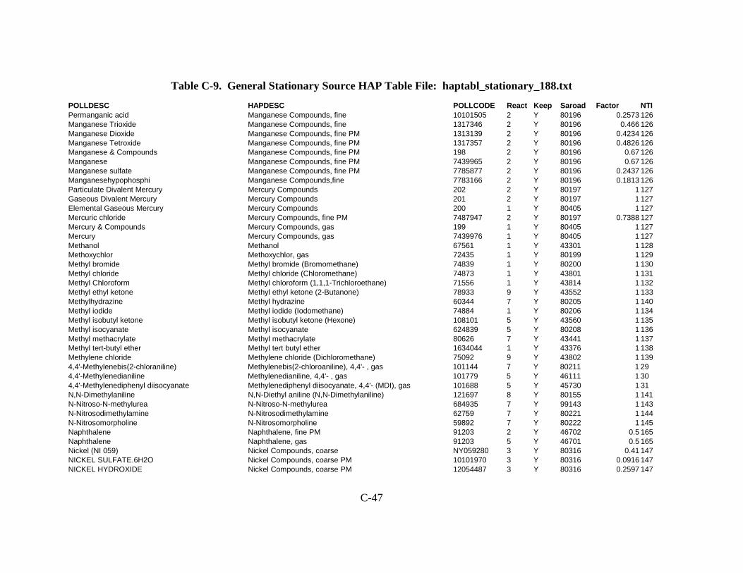
C-47
Table C-9. General Stationary Source HAP Table File: haptabl_stationary_188.txt
POLLDESC HAPDESC POLLCODE React Keep Saroad Factor NTI Permanganic acid Manganese Compounds, fine 10101505 2 Y 80196 0.2573 126 Manganese Trioxide Manganese Compounds, fine 1317346 2 Y 80196 0.466 126 Manganese Dioxide Manganese Compounds, fine PM 1313139 2 Y 80196 0.4234 126 Manganese Tetroxide Manganese Compounds, fine PM 1317357 2 Y 80196 0.4826 126 Manganese & Compounds Manganese Compounds, fine PM 198 2 Y 80196 0.67 126 Manganese Manganese Compounds, fine PM 7439965 2 Y 80196 0.67 126 Manganese sulfate Manganese Compounds, fine PM 7785877 2 Y 80196 0.2437 126 Manganesehypophosphi Manganese Compounds,fine 7783166 2 Y 80196 0.1813 126 Particulate Divalent Mercury Mercury Compounds 202 2 Y 80197 1 127 Gaseous Divalent Mercury Mercury Compounds 201 2 Y 80197 1 127 Elemental Gaseous Mercury Mercury Compounds 200 1 Y 80405 1 127 Mercuric chloride Mercury Compounds, fine PM 7487947 2 Y 80197 0.7388 127 Mercury & Compounds Mercury Compounds, gas 199 1 Y 80405 1 127 Mercury Mercury Compounds, gas 7439976 1 Y 80405 1 127 Methanol Methanol 67561 1 Y 43301 1 128 Methoxychlor Methoxychlor, gas 72435 1 Y 80199 1 129 Methyl bromide Methyl bromide (Bromomethane) 74839 1 Y 80200 1 130 Methyl chloride Methyl chloride (Chloromethane) 74873 1 Y 43801 1 131 Methyl Chloroform Methyl chloroform (1,1,1-Trichloroethane) 71556 1 Y 43814 1 132 Methyl ethyl ketone Methyl ethyl ketone (2-Butanone) 78933 9 Y 43552 1 133 Methylhydrazine Methyl hydrazine 60344 7 Y 80205 1 140 Methyl iodide Methyl iodide (Iodomethane) 74884 1 Y 80206 1 134 Methyl isobutyl ketone Methyl isobutyl ketone (Hexone) 108101 5 Y 43560 1 135 Methyl isocyanate Methyl isocyanate 624839 5 Y 80208 1 136 Methyl methacrylate Methyl methacrylate 80626 7 Y 43441 1 137 Methyl tert-butyl ether Methyl tert butyl ether 1634044 1 Y 43376 1 138 Methylene chloride Methylene chloride (Dichloromethane) 75092 9 Y 43802 1 139 4,4'-Methylenebis(2-chloraniline) Methylenebis(2-chloroaniline), 4,4'- , gas 101144 7 Y 80211 1 29 4,4'-Methylenedianiline Methylenedianiline, 4,4'- , gas 101779 5 Y 46111 1 30 4,4'-Methylenediphenyl diisocyanate Methylenediphenyl diisocyanate, 4,4'- (MDI), gas 101688 5 Y 45730 1 31 N,N-Dimethylaniline N,N-Diethyl aniline (N,N-Dimethylaniline) 121697 8 Y 80155 1 141 N-Nitroso-N-methylurea N-Nitroso-N-methylurea 684935 7 Y 99143 1 143 N-Nitrosodimethylamine N-Nitrosodimethylamine 62759 7 Y 80221 1 144 N-Nitrosomorpholine N-Nitrosomorpholine 59892 7 Y 80222 1 145 Naphthalene Naphthalene, fine PM 91203 2 Y 46702 0.5 165 Naphthalene Naphthalene, gas 91203 5 Y 46701 0.5 165 Nickel (NI 059) Nickel Compounds, coarse NY059280 3 Y 80316 0.41 147 NICKEL SULFATE.6H2O Nickel Compounds, coarse PM 10101970 3 Y 80316 0.0916 147 NICKEL HYDROXIDE Nickel Compounds, coarse PM 12054487 3 Y 80316 0.2597 147

C-48
Table C-9. General Stationary Source HAP Table File: haptabl_stationary_188.txt
POLLDESC HAPDESC POLLCODE React Keep Saroad Factor NTI NICKEL NITRATE Nickel Compounds, coarse PM 13138459 3 Y 80316 0.1317 147 Nickel oxide Nickel Compounds, coarse PM 1313991 3 Y 80316 0.3223 147 NICKEL(111) OXIDE Nickel Compounds, coarse PM 1314063 3 Y 80316 0.2911 147 NICKEL BROMIDE NIBR2 Nickel Compounds, coarse PM 13462889 3 Y 80316 0.1102 147 Nickel carbonyl Nickel Compounds, coarse PM 13463393 3 Y 80316 0.141 147 NICKEL SULFAMATE Nickel Compounds, coarse PM 13770893 3 Y 80316 0.0959 147 Nickel & Compounds Nickel Compounds, coarse PM 226 3 Y 80316 0.41 147 Nickel acetate Nickel Compounds, coarse PM 373024 3 Y 80316 0.1362 147 Nickel Nickel Compounds, coarse PM 7440020 3 Y 80316 0.41 147 NICKEL CHLORIDE Nickel Compounds, coarse PM 7718549 3 Y 80316 0.1857 147 NICKEL SULFATE Nickel Compounds, coarse PM 7786814 3 Y 80316 0.1556 147 Nickel (NI 059) Nickel Compounds, fine NY059280 2 Y 80216 0.59 147 NICKEL SULFATE.6H2O Nickel Compounds, fine PM 10101970 2 Y 80216 0.1318 147 NICKEL HYDROXIDE Nickel Compounds, fine PM 12054487 2 Y 80216 0.3736 147 NICKEL NITRATE Nickel Compounds, fine PM 13138459 2 Y 80216 0.1896 147 Nickel oxide Nickel Compounds, fine PM 1313991 2 Y 80216 0.4637 147 NICKEL(111) OXIDE Nickel Compounds, fine PM 1314063 2 Y 80216 0.4189 147 NICKEL BROMIDE NIBR2 Nickel Compounds, fine PM 13462889 2 Y 80216 0.1585 147 NICKEL SULFAMATE Nickel Compounds, fine PM 13770893 2 Y 80216 0.1381 147 Nickel & Compounds Nickel Compounds, fine PM 226 2 Y 80216 0.59 147 Nickel acetate Nickel Compounds, fine PM 373024 2 Y 80216 0.1959 147 Nickel Nickel Compounds, fine PM 7440020 2 Y 80216 0.59 147 NICKEL CHLORIDE Nickel Compounds, fine PM 7718549 2 Y 80216 0.2673 147 NICKEL SULFATE Nickel Compounds, fine PM 7786814 2 Y 80216 0.2238 147 Nickel carbonyl Nickel Compounds, fine PM 13463393 2 Y 80216 0.2029 147 Nitrobenzene Nitrobenzene 98953 4 Y 45702 1 148 4-Nitrobiphenyl Nitrobiphenyl, 4- 92933 1 Y 99035 1 35 4-Nitrophenol Nitrophenol, 4- 100027 4 Y 80218 1 36 2-Nitropropane Nitropropane, 2- 79469 4 Y 80219 1 25 Anthracene(16PAH) POM, Group 2: no URE data 120127 2 Y 72002 1 165 Dibenzo[a,i]pyrene POM, Group 4: 5.0E-3 < URE <= 5.0E-2 189559 2 Y 74002 1 165 D[a,h]pyrene POM, Group 4: 5.0E-3 < URE <= 5.0E-2 189640 2 Y 74002 1 165 D[a,e]pyrene POM, Group 5: 5.0E-4 < URE <= 5.0E-3 192654 2 Y 75002 1 165 Benzo[e]pyrene POM, Group 2: no URE data 192972 2 Y 72002 1 165 Perylene POM, Group 2: no URE data 198550 2 Y 72002 1 165 B[j]fluoranthen POM, Group 6: 5.0E-5 < URE <= 5.0E-4 205823 2 Y 76002 1 165 Acenaphthylene(16PAH) POM, Group 2: no URE data 208968 2 Y 72002 1 165 D[a,j]acridine POM, Group 6: 5.0E-5 < URE <= 5.0E-4 224420 2 Y 76002 1 165 5-Methylchrysene POM, Group 5: 5.0E-4 < URE <= 5.0E-3 3697243 2 Y 75002 1 165

C-49
Table C-9. General Stationary Source HAP Table File: haptabl_stationary_188.txt
POLLDESC HAPDESC POLLCODE React Keep Saroad Factor NTI 3-Methylcholanthrene POM, Group 4: 5.0E-3 < URE <= 5.0E-2 56495 2 Y 74002 1 165 7,12-Dimethylbenz[a]anthracene POM, Group 3: 5.0E-2 < URE <= 5.0E-1 57976 2 Y 73002 1 165 Acenaphthene(16PAH) POM, Group 2: no URE data 83329 2 Y 72002 1 165 2-Methylnaphthalene POM, Group 2: no URE data 91576 2 Y 72002 1 165 Benzo[b+k]fluoranthene(7PAH) POM, Group 6: 5.0E-5 < URE <= 5.0E-4 102 2 Y 76002 1 165 Benzo[g,h,i,]perylene(16PAH) POM, Group 2: no URE data 191242 2 Y 72002 1 165 Indeno[1,2,3-c,d]pyrene(7PAH) POM, Group 6: 5.0E-5 < URE <= 5.0E-4 193395 2 Y 76002 1 165 Benzo[b]fluoranthene(7PAH) POM, Group 6: 5.0E-5 < URE <= 5.0E-4 205992 2 Y 76002 1 165 Benzo[k]fluoranthene(7PAH) POM, Group 6: 5.0E-5 < URE <= 5.0E-4 207089 2 Y 76002 1 165 Chrysene(7PAH) POM, Group 7: 5.0E-6 < URE <= 5.0E-5 218019 2 Y 77002 1 165 7-PAH POM, Group 8: Unspeciated (7-PAH only) 75 2 Y 78002 1 165 PAH, total POM, Group 1: Unspeciated 234 2 Y 71002 1 165 Polycyclic Organic Matter POM, Group 1: Unspeciated 246 2 Y 71002 1 165 Benzo[a]pyrene(7PAH) POM, Group 5: 5.0E-4 < URE <= 5.0E-3 50328 2 Y 75002 1 165 Dibenzo[a,h]anthracene(7PAH) POM, Group 5: 5.0E-4 < URE <= 5.0E-3 53703 2 Y 75002 1 165 Benz[a]anthracene(7PAH) POM, Group 6: 5.0E-5 < URE <= 5.0E-4 56553 2 Y 76002 1 165 16-PAH - 7-PAH POM, Group 1: Unspeciated 75040 2 Y 71002 1 165 16-PAH POM, Group 1: Unspeciated 40 2 Y 71002 1 165 Fluoranthene(16PAH) POM, Group 2: no URE data 206440 2 Y 72002 1 165 Fluorene(16PAH) POM, Group 2: no URE data 86737 2 Y 72002 1 165 Phenanthrene(16PAH) POM, Group 2: no URE data 85018 2 Y 72002 1 165 Pyrene(16PAH) POM, Group 2: no URE data 129000 2 Y 72002 1 165 Benzofluoranthenes(7PAH) POM, Group 2: no URE data 56832736 2 Y 72002 1 165 2-Chloronaphthalene POM, Group 2: no URE data 91587 2 Y 72002 1 165 Parathion Parathion, gas 56382 7 Y 80223 1 156 Pentachloronitrobenzene Pentachloronitrobenzene (Quintobenzene), gas 82688 1 Y 80224 1 157 Pentachlorophenol Pentachlorophenol, gas 87865 1 Y 80225 1 158 Phenol Phenol 108952 5 Y 45300 1 159 p-Phenylenediamine Phenylenediamine, p- 106503 7 Y 80227 1 154 Phosgene Phosgene 75445 9 Y 80228 1 160 Phosphine Phosphine 7803512 5 Y 99161 1 161 Phosphorus Phosphorus 7723140 2 Y 80229 1 162 Phosphorus Oxychloride Phosphorus Compounds, nonHAP 10025873 2 N 1 Triphenyl phosphite Phosphorus Compounds, nonHAP 101020 2 N 1 Triphenyl phosphate Phosphorus Compounds, nonHAP 115866 2 N 1 Phosphorus Pentoxide Phosphorus Compounds, nonHAP 1314563 2 N 1 PHOSPHOROTHIOIC ACID Phosphorus Compounds, nonHAP 2921882 2 N 1 Phosphoric Acid Phosphorus Compounds, nonHAP 7664382 2 N 1 Phosphorus Trichloride Phosphorus Compounds, nonHAP 7719122 2 N 1
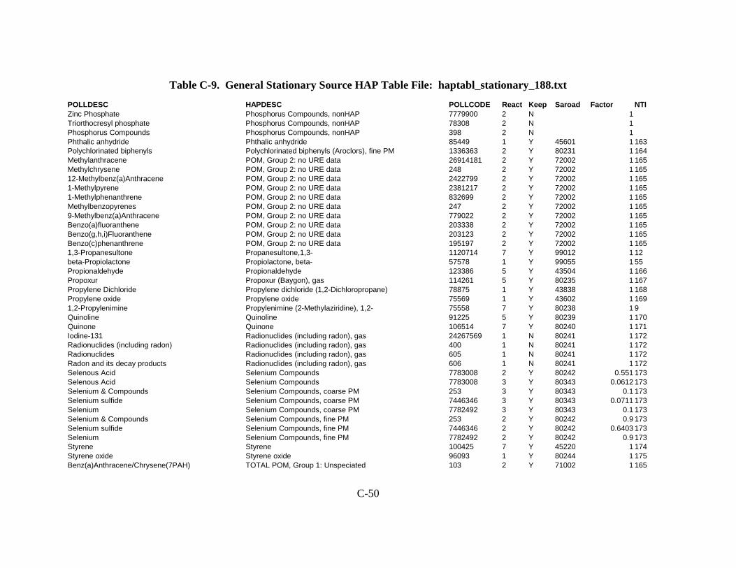
C-50
Table C-9. General Stationary Source HAP Table File: haptabl_stationary_188.txt
POLLDESC HAPDESC POLLCODE React Keep Saroad Factor NTI Zinc Phosphate Phosphorus Compounds, nonHAP 7779900 2 N 1 Triorthocresyl phosphate Phosphorus Compounds, nonHAP 78308 2 N 1 Phosphorus Compounds Phosphorus Compounds, nonHAP 398 2 N 1 Phthalic anhydride Phthalic anhydride 85449 1 Y 45601 1 163 Polychlorinated biphenyls Polychlorinated biphenyls (Aroclors), fine PM 1336363 2 Y 80231 1 164 Methylanthracene POM, Group 2: no URE data 26914181 2 Y 72002 1 165 Methylchrysene POM, Group 2: no URE data 248 2 Y 72002 1 165 12-Methylbenz(a)Anthracene POM, Group 2: no URE data 2422799 2 Y 72002 1 165 1-Methylpyrene POM, Group 2: no URE data 2381217 2 Y 72002 1 165 1-Methylphenanthrene POM, Group 2: no URE data 832699 2 Y 72002 1 165 Methylbenzopyrenes POM, Group 2: no URE data 247 2 Y 72002 1 165 9-Methylbenz(a)Anthracene POM, Group 2: no URE data 779022 2 Y 72002 1 165 Benzo(a)fluoranthene POM, Group 2: no URE data 203338 2 Y 72002 1 165 Benzo(g,h,i)Fluoranthene POM, Group 2: no URE data 203123 2 Y 72002 1 165 Benzo(c)phenanthrene POM, Group 2: no URE data 195197 2 Y 72002 1 165 1,3-Propanesultone Propanesultone,1,3- 1120714 7 Y 99012 1 12 beta-Propiolactone Propiolactone, beta- 57578 1 Y 99055 1 55 Propionaldehyde Propionaldehyde 123386 5 Y 43504 1 166 Propoxur Propoxur (Baygon), gas 114261 5 Y 80235 1 167 Propylene Dichloride Propylene dichloride (1,2-Dichloropropane) 78875 1 Y 43838 1 168 Propylene oxide Propylene oxide 75569 1 Y 43602 1 169 1,2-Propylenimine Propylenimine (2-Methylaziridine), 1,2- 75558 7 Y 80238 1 9 Quinoline Quinoline 91225 5 Y 80239 1 170 Quinone Quinone 106514 7 Y 80240 1 171 Iodine-131 Radionuclides (including radon), gas 24267569 1 N 80241 1 172 Radionuclides (including radon) Radionuclides (including radon), gas 400 1 N 80241 1 172 Radionuclides Radionuclides (including radon), gas 605 1 N 80241 1 172 Radon and its decay products Radionuclides (including radon), gas 606 1 N 80241 1 172 Selenous Acid Selenium Compounds 7783008 2 Y 80242 0.551 173 Selenous Acid Selenium Compounds 7783008 3 Y 80343 0.0612 173 Selenium & Compounds Selenium Compounds, coarse PM 253 3 Y 80343 0.1 173 Selenium sulfide Selenium Compounds, coarse PM 7446346 3 Y 80343 0.0711 173 Selenium Selenium Compounds, coarse PM 7782492 3 Y 80343 0.1 173 Selenium & Compounds Selenium Compounds, fine PM 253 2 Y 80242 0.9 173 Selenium sulfide Selenium Compounds, fine PM 7446346 2 Y 80242 0.6403 173 Selenium Selenium Compounds, fine PM 7782492 2 Y 80242 0.9 173 Styrene Styrene 100425 7 Y 45220 1 174 Styrene oxide Styrene oxide 96093 1 Y 80244 1 175 Benz(a)Anthracene/Chrysene(7PAH) TOTAL POM, Group 1: Unspeciated 103 2 Y 71002 1 165
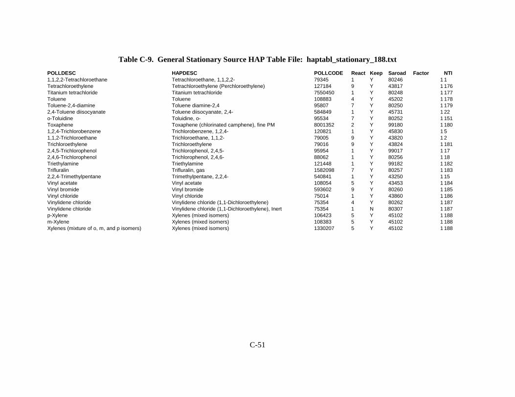
C-51
Table C-9. General Stationary Source HAP Table File: haptabl_stationary_188.txt
POLLDESC HAPDESC POLLCODE React Keep Saroad Factor NTI 1,1,2,2-Tetrachloroethane Tetrachloroethane, 1,1,2,2- 79345 1 Y 80246 1 1 Tetrachloroethylene Tetrachloroethylene (Perchloroethylene) 127184 9 Y 43817 1 176 Titanium tetrachloride Titanium tetrachloride 7550450 1 Y 80248 1 177 Toluene Toluene 108883 4 Y 45202 1 178 Toluene-2,4-diamine Toluene diamine-2,4 95807 7 Y 80250 1 179 2,4-Toluene diisocyanate Toluene diisocyanate, 2,4- 584849 1 Y 45731 1 22 o-Toluidine Toluidine, o- 95534 7 Y 80252 1 151 Toxaphene Toxaphene (chlorinated camphene), fine PM 8001352 2 Y 99180 1 180 1,2,4-Trichlorobenzene Trichlorobenzene, 1,2,4- 120821 1 Y 45830 1 5 1,1,2-Trichloroethane Trichloroethane, 1,1,2- 79005 9 Y 43820 1 2 Trichloroethylene Trichloroethylene 79016 9 Y 43824 1 181 2,4,5-Trichlorophenol Trichlorophenol, 2,4,5- 95954 1 Y 99017 1 17 2,4,6-Trichlorophenol Trichlorophenol, 2,4,6- 88062 1 Y 80256 1 18 Triethylamine Triethylamine 121448 1 Y 99182 1 182 Trifluralin Trifluralin, gas 1582098 7 Y 80257 1 183 2,2,4-Trimethylpentane Trimethylpentane, 2,2,4- 540841 1 Y 43250 1 15 Vinyl acetate Vinyl acetate 108054 5 Y 43453 1 184 Vinyl bromide Vinyl bromide 593602 9 Y 80260 1 185 Vinyl chloride Vinyl chloride 75014 1 Y 43860 1 186 Vinylidene chloride Vinylidene chloride (1,1-Dichloroethylene) 75354 4 Y 80262 1 187 Vinylidene chloride Vinylidene chloride (1,1-Dichloroethylene), Inert 75354 1 N 80307 1 187 p-Xylene Xylenes (mixed isomers) 106423 5 Y 45102 1 188 m-Xylene Xylenes (mixed isomers) 108383 5 Y 45102 1 188 Xylenes (mixture of o, m, and p isomers) Xylenes (mixed isomers) 1330207 5 Y 45102 1 188

C-52
Table C-10. General Onroad Mobile HAP Table File: haptabl_onroad_toxwt.txt
POLLDESC HAPDESC POLLCODE React Keep Saroad Factor NTI 2,3,7,8-TCDD TEQ Dioxins/Furans as 2,3,7,8TCCD TEQ, Lower Bound, Fi 600 2 N 80412 1 903 2,3,7,8-TCDD TEQ Dioxins/Furans as 2,3,7,8TCCD TEQ, Upper Bound, Fi 600 2 N 80245 1 903 7-PAH 7-PAH, fine PM 75 2 Y 80233 1 165 7-PAH POM, Group 8: Unspeciated (7-PAH only) 75 2 Y 78002 1 165 Acenaphthene POM, Group 2: no URE data 83329 2 Y 72002 1 165 Acenaphthylene POM, Group 2: no URE data 208968 2 Y 72002 1 165 Anthracene POM, Group 2: no URE data 120127 2 Y 72002 1 165 Benz[a]anthracene POM, Group 6: 5.0E-5 < URE <= 5.0E-4 56553 2 Y 76002 1 165 Benz[a]anthracene 7-PAH, fine PM 56553 2 Y 80233 1 165 Benzo[b]fluoranthene POM, Group 6: 5.0E-5 < URE <= 5.0E-4 205992 2 Y 76002 1 165 Benzo[b]fluoranthene 7-PAH, fine PM 205992 2 Y 80233 1 165 Benzo[k]fluoranthene POM, Group 6: 5.0E-5 < URE <= 5.0E-4 207089 2 Y 76002 1 165 Benzo[k]fluoranthene 7-PAH, fine PM 207089 2 Y 80233 1 165 Benzo[g,h,i,]perylene POM, Group 2: no URE data 191242 2 Y 72002 1 165 Benzo[a]pyrene POM, Group 5: 5.0E-4 < URE <= 5.0E-3 50328 2 Y 75002 1 165 Benzo[a]pyrene 7-PAH, fine PM 50328 2 Y 80233 1 165 Benzo[e]pyrene POM, Group 2: no URE data 192972 2 Y 72002 1 165 Chrysene POM, Group 7: 5.0E-6 < URE <= 5.0E-5 218019 2 Y 77002 1 165 Chrysene 7-PAH, fine PM 218019 2 Y 80233 1 165 Dibenzo[a,h]anthracene POM, Group 5: 5.0E-4 < URE <= 5.0E-3 53703 2 Y 75002 1 165 Dibenzo[a,h]anthracene 7-PAH, fine PM 53703 2 Y 80233 1 165 Fluoranthene POM, Group 2: no URE data 206440 2 Y 72002 1 165 Fluorene POM, Group 2: no URE data 86737 2 Y 72002 1 165 Indeno[1,2,3-c,d]pyrene POM, Group 6: 5.0E-5 < URE <= 5.0E-4 193395 2 Y 76002 1 165 Indeno[1,2,3-c,d]pyrene 7-PAH, fine PM 193395 2 Y 80233 1 165 Phenanthrene POM, Group 2: no URE data 85018 2 Y 72002 1 165 Pyrene POM, Group 2: no URE data 129000 2 Y 72002 1 165 Naphthalene Naphthalene, fine PM 91203 2 Y 46702 0.5 165 Naphthalene Naphthalene, gas 91203 5 Y 46701 0.5 165 Acetaldehyde Acetaldehyde 75070 5 Y 43503 1 37 Acrolein Acrolein 107028 5 Y 43505 1 41 Antimony Antimony Compounds, coarse PM 7440360 3 Y 80311 0.31 47 Antimony Antimony Compounds, fine PM 7440360 2 Y 80111 0.69 47 Arsenic Arsenic (inorganic, incl. unknown arsine), coarse 7440382 3 Y 70312 0.1 48 Arsenic Arsenic (inorganic, incl. unknown arsine), fine 7440382 2 Y 70112 0.9 48 Arsenic Compds. (inorganic incl. unknown arsin Arsenic (inorganic, incl. unknown arsine), coarse 93 3 Y 70312 0.1 48 Arsenic Compds. (inorganic incl. unknown arsin Arsenic (inorganic, incl. unknown arsine), fine 93 2 Y 70112 0.9 48 Benzene Benzene (including benzene from gasoline) 71432 1 Y 45201 1 50

C-53
Table C-10. General Onroad Mobile HAP Table File: haptabl_onroad_toxwt.txt POLLDESC HAPDESC POLLCODE React Keep Saroad Factor NTI 1,3-Butadiene Butadiene, 1,3- 106990 7 Y 43218 1 10 1,3-Butadiene Acrolein precusor - inert surrogate 106990 1 Y 80302 1 Cadmium Cadmium Compounds, coarse PM 7440439 3 Y 80324 0.62 60 Cadmium Cadmium Compounds, fine PM 7440439 2 Y 80124 0.38 60 Chlorine Chlorine 7782505 1 N 80135 1 70 Chromium III Chromium III Compounds, coarse PM 16065831 3 Y 59993 0.14 77 Chromium III Chromium III Compounds, fine PM 16065831 2 Y 59992 0.86 77 Chromium +6 Chromium VI Compounds, coarse PM 18540299 3 Y 69993 0.14 77 Chromium +6 Chromium VI Compounds, fine PM 18540299 2 Y 69992 0.86 77 Chromium & Compounds Chromium Compounds, coarse PM 136 3 Y 80341 0.14 77 Chromium & Compounds Chromium Compounds, fine PM 136 2 Y 80141 0.86 77 Chromium Chromium Compounds, coarse PM 7440473 3 Y 80341 0.14 77 Chromium Chromium Compounds, fine PM 7440473 2 Y 80141 0.86 77 Cobalt Cobalt Compounds, coarse PM 7440484 3 N 80342 0.19 78 Cobalt Cobalt Compounds, fine PM 7440484 2 N 80142 0.81 78 Cumene Cumene 98828 9 N 45210 1 81 Diesel PM, coarse Diesel, coarse PM dpmcoarse 3 Y 80401 1 Diesel PM, fine Diesel, fine PM dpmfine 2 Y 80400 1 Diesel PM Diesel, coarse PM 80400 3 Y 80401 0.08 Diesel PM Diesel, fine PM 80400 2 Y 80400 0.92 Dioxins/Furans as TEQ Dioxins/Furans as 2,3,7,8TCCD TEQ, Lower Bound, Fine 701 2 N 80412 1 902 Dioxins/Furans as TEQ Dioxins/Furans as 2,3,7,8TCCD TEQ, Upper Bound, Fine 701 2 N 80245 1 902 Ethyl Benzene Ethylbenzene 100414 4 Y 45203 1 98 Formaldehyde Formaldehyde 50000 5 Y 43502 1 107 Hexane Hexane 110543 9 Y 43231 1 116 Lead & Compounds Lead Compounds, coarse PM 195 3 Y 80393 0.24 122 Lead & Compounds Lead Compounds, fine PM 195 2 Y 80193 0.76 122 Lead Lead Compounds, coarse PM 7439921 3 Y 80393 0.24 122 Lead Lead Compounds, fine PM 7439921 2 Y 80193 0.76 122 Manganese & Compounds Manganese Compounds, coarse PM 198 3 Y 80396 0.36 126 Manganese & Compounds Manganese Compounds, fine PM 198 2 Y 80196 0.64 126 Manganese Manganese Compounds, coarse PM 7439965 3 Y 80396 0.36 126 Manganese Manganese Compounds, fine PM 7439965 2 Y 80196 0.64 126 Mercury & Compounds Mercury Compounds, fine PM 199 2 Y 80197 1 127 Mercury Mercury Compounds, fine PM 7439976 2 Y 80197 1 127 Methanol Methanol 67561 1 N 43301 1 128 Methyl ethyl ketone Methyl ethyl ketone (2-Butanone) 78933 9 N 43552 1 133 Methyl tert-butyl ether Methyl tert butyl ether 1634044 1 Y 43376 1 138 Nickel & Compounds Nickel Compounds, coarse PM 226 3 Y 80316 0.17 147

C-54
Table C-10. General Onroad Mobile HAP Table File: haptabl_onroad_toxwt.txt POLLDESC HAPDESC POLLCODE React Keep Saroad Factor NTI Nickel & Compounds Nickel Compounds, fine PM 226 2 Y 80216 0.83 147 Nickel Nickel Compounds, coarse PM 7440020 3 Y 80316 0.17 147 Nickel Nickel Compounds, fine PM 7440020 2 Y 80216 0.83 147 Phosphorus Phosphorus 7723140 2 N 80229 1 162 16-PAH POM, Group 1: unspeciated 40 2 Y 71002 1 165 Propionaldehyde Propionaldehyde 123386 5 Y 43504 1 166 Selenium Selenium Compounds, fine PM 7782492 2 N 80242 1 173 Styrene Styrene 100425 7 Y 45220 1 174 Toluene Toluene 108883 4 Y 45202 1 178 2,2,4-Trimethylpentane Trimethylpentane, 2,2,4- 540841 1 Y 43250 1 15 Xylenes (mixture of o, m, and p isomers) Xylenes (mixed isomers) 1330207 5 Y 45102 1 188 p-Xylene Xylenes (mixed isomers) 106423 5 Y 45102 1 188 m-Xylene Xylenes (mixed isomers) 108383 5 Y 45102 1 188 o-Xylene Xylenes (mixed isomers) 95476 5 Y 45102 1 188

C-55
Table C-11. General Nonroad Mobile HAP Table File: haptabl_nonroadGEN_toxwt.txt POLLDESC **c/f-split fixed for Cr3&6 HAPDESC POLLCODE React Keep Saroad Factor NTI 7-PAH 7-PAH, fine PM 75 2 Y 80233 1 165 Acetaldehyde Acetaldehyde 75070 5 Y 43503 1 37 Acrolein Acrolein 107028 5 Y 43505 1 41 Antimony Antimony Compounds, coarse PM 7440360 3 Y 80311 0.63 47 Antimony Antimony Compounds, fine PM 7440360 2 Y 80111 0.37 47 Arsenic & Comps (inorganic inc. unknown arsin Arsenic (inorganic, incl. unknown arsine), coarse 93 3 Y 70312 0.17 48 Arsenic & Comps (inorganic inc. unknown arsin Arsenic (inorganic, incl. unknown arsine), fine 93 2 Y 70112 0.83 48 Arsenic Arsenic (inorganic, incl. unknown arsine), coarse 7440382 3 Y 70312 0.17 48 Arsenic Arsenic (inorganic, incl. unknown arsine), fine 7440382 2 Y 70112 0.83 48 Benzene Benzene (including benzene from gasoline) 71432 1 Y 45201 1 50 Beryllium & Compounds Beryllium Compounds, coarse PM 109 3 Y 80318 0.61 54 Beryllium & Compounds Beryllium Compounds, fine PM 109 2 Y 80118 0.39 54 Beryllium Beryllium Compounds, coarse PM 7440417 3 Y 80318 0.61 54 Beryllium Beryllium Compounds, fine PM 7440417 2 Y 80118 0.39 54 1,3-Butadiene Butadiene, 1,3- 106990 7 Y 43218 1 10 1,3-Butadiene Acrolein precusor - inert surrogate 106990 1 Y 80302 1 10 Cadmium & Compounds Cadmium Compounds, coarse PM 125 3 Y 80324 0.62 60 Cadmium & Compounds Cadmium Compounds, fine PM 125 2 Y 80124 0.38 60 Cadmium Cadmium Compounds, coarse PM 7440439 3 Y 80324 0.62 60 Cadmium Cadmium Compounds, fine PM 7440439 2 Y 80124 0.38 60 Chlorine Chlorine 7782505 1 Y 80135 1 70 Chlorobenzene Chlorobenzene 108907 1 Y 45801 1 72 Chromium III Chromium III Compounds, coarse PM 16065831 3 Y 59993 0.2 77 Chromium III Chromium III Compounds, fine PM 16065831 2 Y 59992 0.8 77 Chromium +6 Chromium VI Compounds, coarse PM 18540299 3 Y 69993 0.2 77 Chromium +6 Chromium VI Compounds, fine PM 18540299 2 Y 69992 0.8 77 Chromium III Chromium III Compounds, coarse PM 16065831 3 N 80341 0.2 77 Chromium III Chromium III Compounds, fine PM 16065831 2 N 80141 0.8 77 Chromium +6 Chromium VI Compounds, coarse PM 18540299 3 N 80341 0.2 77 Chromium +6 Chromium VI Compounds, fine PM 18540299 2 N 80141 0.8 77 Chromium & Compounds Chromium Compounds, coarse PM 136 3 Y 80341 0.2 77 Chromium & Compounds Chromium Compounds, fine PM 136 2 Y 80141 0.8 77 Chromium Chromium Compounds, coarse PM 7440473 3 Y 80341 0.2 77 Chromium Chromium Compounds, fine PM 7440473 2 Y 80141 0.8 77 Cobalt Cobalt Compounds, coarse PM 7440484 3 Y 80342 0.1 78 Cobalt Cobalt Compounds, fine PM 7440484 2 Y 80142 0.9 78 Cumene Cumene 98828 9 Y 45210 1 81 Diesel PM, coarse Diesel, coarse PM dpmcoarse 3 Y 80401 1

C-56
Table C-11. General Nonroad Mobile HAP Table File: haptabl_nonroadGEN_toxwt.txt POLLDESC **c/f-split fixed for Cr3&6 HAPDESC POLLCODE React Keep Saroad Factor NTI Diesel PM, fine Diesel, fine PM dpmfine 2 Y 80400 1 Diesel PM Diesel, coarse PM 80400 3 Y 80401 0.08 Diesel PM Diesel, fine PM 80400 2 Y 80400 0.92 2,3,7,8-TCDD TEQ Dioxins/Furans as 2,3,7,8TCCD TEQ, Lower Bound, Fi 600 2 N 80412 1 903 2,3,7,8-TCDD TEQ Dioxins/Furans as 2,3,7,8TCCD TEQ, Upper Bound, Fi 600 2 Y 80245 1 903 Ethyl Benzene Ethylbenzene 100414 4 Y 45203 1 98 Formaldehyde Formaldehyde 50000 5 Y 43502 1 107 Hexane Hexane 110543 9 Y 43231 1 116 Lead & Compounds Lead Compounds, coarse PM 195 3 Y 80393 0.12 122 Lead & Compounds Lead Compounds, fine PM 195 2 Y 80193 0.88 122 Lead Lead Compounds, coarse PM 7439921 3 Y 80393 0.12 122 Lead Lead Compounds, fine PM 7439921 2 Y 80193 0.88 122 Manganese & Compounds Manganese Compounds, coarse PM 198 3 Y 80396 0.21 126 Manganese & Compounds Manganese Compounds, fine PM 198 2 Y 80196 0.79 126 Manganese Manganese Compounds, coarse PM 7439965 3 Y 80396 0.33 126 Manganese Manganese Compounds, fine PM 7439965 2 Y 80196 0.67 126 Mercury & Compounds Mercury Compounds, fine PM 199 2 Y 80197 1 127 Mercury Mercury Compounds, fine PM 7439976 2 Y 80197 1 127 Methanol Methanol 67561 1 Y 43301 1 128 Methyl ethyl ketone Methyl ethyl ketone (2-Butanone) 78933 9 Y 43552 1 133 Methyl tert-butyl ether Methyl tert butyl ether 1634044 1 Y 43376 1 138 Nickel & Compounds Nickel Compounds, coarse PM 226 3 Y 80316 0.51 147 Nickel & Compounds Nickel Compounds, fine PM 226 2 Y 80216 0.49 147 Nickel Nickel Compounds, coarse PM 7440020 3 Y 80316 0.51 147 Nickel Nickel Compounds, fine PM 7440020 2 Y 80216 0.49 147 Phenol Phenol 108952 5 Y 45300 1 159 Phosphorus Phosphorus 7723140 2 Y 80229 1 162 16-PAH - 7-PAH POM, Group 1: Unspeciated 75040 2 Y 71002 1 165 16-PAH POM, Group 1: unspeciated 40 2 Y 71002 1 165 7-PAH POM, Group 8: Unspeciated (7-PAH only) 75 2 Y 78002 1 165 Anthracene POM, Group 2: no URE data 120127 2 Y 72002 1 165 Pyrene POM, Group 2: no URE data 129000 2 Y 72002 1 165 Benzo[g,h,i,]perylene POM, Group 2: no URE data 191242 2 Y 72002 1 165 Indeno[1,2,3-c,d]pyrene POM, Group 6: 5.0E-5 < URE <= 5.0E-4 193395 2 Y 76002 1 165 Benzo[b]fluoranthene POM, Group 6: 5.0E-5 < URE <= 5.0E-4 205992 2 Y 76002 1 165 Benzo[k]fluoranthene POM, Group 6: 5.0E-5 < URE <= 5.0E-4 207089 2 Y 76002 1 165 Chrysene POM, Group 7: 5.0E-6 < URE <= 5.0E-5 218019 2 Y 77002 1 165 Benzo[a]pyrene POM, Group 5: 5.0E-4 < URE <= 5.0E-3 50328 2 Y 75002 1 165

C-57
Table C-11. General Nonroad Mobile HAP Table File: haptabl_nonroadGEN_toxwt.txt POLLDESC **c/f-split fixed for Cr3&6 HAPDESC POLLCODE React Keep Saroad Factor NTI Dibenzo[a,h]anthracene POM, Group 5: 5.0E-4 < URE <= 5.0E-3 53703 2 Y 75002 1 165 Benz[a]anthracene POM, Group 6: 5.0E-5 < URE <= 5.0E-4 56553 2 Y 76002 1 165 Acenaphthene POM, Group 2: no URE data 83329 2 Y 72002 1 165 Fluoranthene POM, Group 2: no URE data 206440 2 Y 72002 1 165 Acenaphthylene POM, Group 2: no URE data 208968 2 Y 72002 1 165 Phenanthrene POM, Group 2: no URE data 85018 2 Y 72002 1 165 Naphthalene Naphthalene, fine PM 91203 2 Y 46702 0.5 165 Naphthalene Naphthalene, gas 91203 5 Y 46701 0.5 165 Fluorene POM, Group 2: no URE data 86737 2 Y 72002 1 165 Benzo[a]pyrene 7-PAH, fine PM 50328 2 Y 80233 1 165 Indeno[1,2,3-c,d]pyrene 7-PAH, fine PM 193395 2 Y 80233 1 165 Benzo[b]fluoranthene 7-PAH, fine PM 205992 2 Y 80233 1 165 Benzo[k]fluoranthene 7-PAH, fine PM 207089 2 Y 80233 1 165 Chrysene 7-PAH, fine PM 218019 2 Y 80233 1 165 Dibenzo[a,h]anthracene 7-PAH, fine PM 53703 2 Y 80233 1 165 Benz[a]anthracene 7-PAH, fine PM 56553 2 Y 80233 1 165 Propionaldehyde Propionaldehyde 123386 5 Y 43504 1 166 Selenium & Compounds Selenium Compounds, coarse PM 253 3 Y 80343 0.11 173 Selenium & Compounds Selenium Compounds, fine PM 253 2 Y 80242 0.89 173 Selenium Selenium Compounds, coarse PM 7782492 3 Y 80343 0.11 173 Selenium Selenium Compounds, fine PM 7782492 2 Y 80242 0.89 173 Styrene Styrene 100425 7 Y 45220 1 174 Toluene Toluene 108883 4 Y 45202 1 178 2,2,4-Trimethylpentane Trimethylpentane, 2,2,4- 540841 1 Y 43250 1 15 p-Xylene Xylenes (mixed isomers) 106423 5 Y 45102 1 188 m-Xylene Xylenes (mixed isomers) 108383 5 Y 45102 1 188 Xylenes (mixture of o, m, and p isomers) Xylenes (mixed isomers) 1330207 5 Y 45102 1 188

C-58
Table C-12. Precursor General HAP Table File (used for precursors from all inventories): haptabl_precursor.txt
POLLDESC HAPDESC POLLCODE React Keep Saroad Factor Propene Acetaldehyde precursors-inert surrogate P33 1 Y 80301 0.525Butene, 2- Acetaldehyde precursors-inert surrogate P10 1 Y 80301 1.58Pentene, 2- Acetaldehyde precursors-inert surrogate P19 1 Y 80301 0.63Hexene, 2- Acetaldehyde precursors-inert surrogate P13 1 Y 80301 0.52Heptene, 2- Acetaldehyde precursors-inert surrogate P12 1 Y 80301 0.45Octene, 2- Acetaldehyde precursors-inert surrogate P18 1 Y 80301 0.39Nonene, 2- Acetaldehyde precursors-inert surrogate P17 1 Y 80301 0.63Butene,2-, 2-methyl Acetaldehyde precursors-inert surrogate P16 1 Y 80301 0.945Pentene, 2-, 3-methyl Acetaldehyde precursors-inert surrogate P23 1 Y 80301 0.78Pentene, 2-, 4-methyl Acetaldehyde precursors-inert surrogate P26 1 Y 80301 0.52Ethanol Acetaldehyde precursors-inert surrogate P28 1 Y 80301 0.048Propene Acetaldehyde precursors-reactive surrogate P33 7 Y 80100 0.525Butene, 2- Acetaldehyde precursors-reactive surrogate P10 7 Y 80100 1.58Pentene, 2- Acetaldehyde precursors-reactive surrogate P19 7 Y 80100 0.63Hexene, 2- Acetaldehyde precursors-reactive surrogate P13 7 Y 80100 0.52Heptene, 2- Acetaldehyde precursors-reactive surrogate P12 7 Y 80100 0.45Octene, 2- Acetaldehyde precursors-reactive surrogate P18 7 Y 80100 0.39Nonene, 2- Acetaldehyde precursors-reactive surrogate P17 7 Y 80100 0.63Butene,2-, 2-methyl Acetaldehyde precursors-reactive surrogate P16 7 Y 80100 0.945Pentene, 2-, 3-methyl Acetaldehyde precursors-reactive surrogate P23 7 Y 80100 0.78Pentene, 2-, 4-methyl Acetaldehyde precursors-reactive surrogate P26 7 Y 80100 0.52Ethanol Acetaldehyde precursors-reactive surrogate P28 7 Y 80100 0.048Butadiene, 1,3- Acrolein precusor - inert surrogate 106990 1 Y 80302 1Toluene Cresol Precursors - inert surrogate 108883 1 Y 80306 0.288Toluene Cresol Precursors - reactive surrogate 108883 4 Y 80506 0.288Ethene Formaldehyde precursors-inert surrogate P29 1 Y 80303 0.5136Propene Formaldehyde precursors-inert surrogate P33 1 Y 80303 0.71Butene, 1- Formaldehyde precursors-inert surrogate P01 1 Y 80303 0.54Pentene, 1- Formaldehyde precursors-inert surrogate P07 1 Y 80303 0.43Hexene, 1- Formaldehyde precursors-inert surrogate P04 1 Y 80303 0.36Heptene, 1- Formaldehyde precursors-inert surrogate P03 1 Y 80303 0.31Octene, 1- Formaldehyde precursors-inert surrogate P06 1 Y 80303 0.27Nonene, 1- Formaldehyde precursors-inert surrogate P05 1 Y 80303 0.24Decene, 1- Formaldehyde precursors-inert surrogate P02 1 Y 80303 0.21Propene, 2-methyl (Isobutene) Formaldehyde precursors-inert surrogate P30 1 Y 80303 0.864Butene, 1-, 2-methyl Formaldehyde precursors-inert surrogate P14 1 Y 80303 0.688Butadiene, 1,3- Formaldehyde precursors-inert surrogate 106990 1 Y 80303 1.12Butene, 1-, 3-methyl Formaldehyde precursors-inert surrogate P21 1 Y 80303 0.43Pentene, 1-, 3-methyl Formaldehyde precursors-inert surrogate P22 1 Y 80303 0.36Butene, 1-, 2,3-dimethyl Formaldehyde precursors-inert surrogate P08 1 Y 80303 0.576Isoprene Formaldehyde precursors-inert surrogate P32 1 Y 80303 0.8844Butene, 1-, 2-ethyl Formaldehyde precursors-inert surrogate P11 1 Y 80303 0.576Pentene, 1-, 2-methyl Formaldehyde precursors-inert surrogate P15 1 Y 80303 0.576Pentene, 1-, 4-methyl Formaldehyde precursors-inert surrogate P25 1 Y 80303 0.36Pentene, 1-, 2,4,4-trimethyl Formaldehyde precursors-inert surrogate P09 1 Y 80303 0.432Acetaldehyde Formaldehyde precursors-inert surrogate 75070 1 Y 80303 0.34MTBE Formaldehyde precursors-inert surrogate 1634044 1 Y 80303 0.0143Methanol Formaldehyde precursors-inert surrogate 67561 1 Y 80303 0.0282Ethene Formaldehyde precursors-reactive surrogate P29 6 Y 80180 0.5136Propene Formaldehyde precursors-reactive surrogate P33 6 Y 80180 0.71Butene, 1- Formaldehyde precursors-reactive surrogate P01 6 Y 80180 0.54Pentene, 1- Formaldehyde precursors-reactive surrogate P07 6 Y 80180 0.43Hexene, 1- Formaldehyde precursors-reactive surrogate P04 6 Y 80180 0.36Heptene, 1- Formaldehyde precursors-reactive surrogate P03 6 Y 80180 0.31Octene, 1- Formaldehyde precursors-reactive surrogate P06 6 Y 80180 0.27

C-59
Table C-12. Precursor General HAP Table File (used for precursors from all inventories): haptabl_precursor.txt
POLLDESC HAPDESC POLLCODE React Keep Saroad Factor Nonene, 1- Formaldehyde precursors-reactive surrogate P05 6 Y 80180 0.24Decene, 1- Formaldehyde precursors-reactive surrogate P02 6 Y 80180 0.21Propene, 2-methyl (Isobutene) Formaldehyde precursors-reactive surrogate P30 6 Y 80180 0.864Butene, 1-, 2-methyl Formaldehyde precursors-reactive surrogate P14 6 Y 80180 0.688Butadiene, 1,3- Formaldehyde precursors-reactive surrogate 106990 6 Y 80180 1.12Butene, 1-, 3-methyl Formaldehyde precursors-reactive surrogate P21 6 Y 80180 0.43Pentene, 1-, 3-methyl Formaldehyde precursors-reactive surrogate P22 6 Y 80180 0.36Butene, 1-, 2,3-dimethyl Formaldehyde precursors-reactive surrogate P08 6 Y 80180 0.576Isoprene Formaldehyde precursors-reactive surrogate P32 6 Y 80180 0.8844Butene, 1-, 2-ethyl Formaldehyde precursors-reactive surrogate P11 6 Y 80180 0.576Pentene, 1-, 2-methyl Formaldehyde precursors-reactive surrogate P15 6 Y 80180 0.576Pentene, 1-, 4-methyl Formaldehyde precursors-reactive surrogate P25 6 Y 80180 0.36Pentene, 1-, 2,4,4-trimethyl Formaldehyde precursors-reactive surrogate P09 6 Y 80180 0.432Acetaldehyde Formaldehyde precursors-reactive surrogate 75070 6 Y 80180 0.34MTBE Formaldehyde precursors-reactive surrogate 1634044 6 Y 80180 0.0143Methanol Formaldehyde precursors-reactive surrogate 67561 6 Y 80180 0.0282Butene, 1-, 2-methyl MEK precursors-inert surrogate P14 1 Y 80304 0.86Butane MEK precursors-inert surrogate P27 1 Y 80304 0.0309Isopentane MEK precursors-inert surrogate P31 1 Y 80304 0.0249Pentane, 3-methyl MEK precursors-inert surrogate P24 1 Y 80304 0.0213Butene, 1-, 2-methyl MEK precursors-reactive surrogate P14 7 Y 80204 0.86Butane MEK precursors-reactive surrogate P27 7 Y 80204 0.0309Isopentane MEK precursors-reactive surrogate P31 7 Y 80204 0.0249Pentane, 3-methyl MEK precursors-reactive surrogate P24 7 Y 80204 0.0213Methylene Chloride Phosgene precursors - inert surrogate 75092 1 Y 80350 1.16Tetrachloroethylene Phosgene precursors - inert surrogate 127184 1 Y 80350 0.2816Trichloroethylene Phosgene precursors - inert surrogate 79016 1 Y 80350 0.2988Vinylidene Chloride Phosgene precursors - inert surrogate 75354 1 Y 80350 0.7446Vinylidene Chloride Phosgene precursors - reactive 4 surrogate 75354 4 Y 80550 0.7446Methylene Chloride Phosgene precursors - reactive 9 surrogate 75092 9 Y 80450 1.16Tetrachloroethylene Phosgene precursors - reactive 9 surrogate 127184 9 Y 80450 0.2816Trichloroethylene Phosgene precursors - reactive 9 surrogate 79016 9 Y 80450 0.2988Butene, 1- Propionaldehyde precursors-inert surrogate P01 1 Y 80305 0.52Pentene, 2- Propionaldehyde precursors-inert surrogate P19 1 Y 80305 0.83Hexene, 3- Propionaldehyde precursors-inert surrogate P20 1 Y 80305 1.38Butene, 1- Propionaldehyde precursors-reactive surrogate P01 7 Y 80234 0.52Pentene, 2- Propionaldehyde precursors-reactive surrogate P19 7 Y 80234 0.83Hexene, 3- Propionaldehyde precursors-reactive surrogate P20 7 Y 80234 1.38
C.4.3 How we developed the Specific HAP Table File (Keyword SPECHAP): haptabl_SPEC.txt
The specific HAP table is new to Version 3 of EMS-HAP. We developed haptabl_SPEC.txt by gathering data from engineers who work on specific source categories that emit chromium. The data were gathered during the spring and summer of 2003. Chuck French, Emission Standards Division (ESD) in OAQPS led the data gathering effort from ESD engineers, and Gene Riley, Emissions, Monitoring and Analysis Division (EMAD) provided data from his testing experiences. We also examined speciated chromium data in the 1996 NTI to determine whether a category-based speciation factor could be determined. The following presents the results of this study:

C-60
Category hexavalent chromium Justification
Aerospace 3% Assume 3% is Cr VI, this appears to be a conservative, but reasonable estimate based on input from Tony Wayne (ESD Project Manager).
Asphalt Paving Mixtures (Hot Batch Plants - virgin not recycle materials) 3%
MAX of Gene Riley’s (EMAD) recommended range: 1% to 3% Cr VI emissions based on prior experience. This estimated range is dependent upon the Cr content for the raw materials being processed
Asphalt Roofing and Processing 5% MAX of two processes within this category
Asphalt Roofing and Processing (Saturate & Coating Blowing Stills) 5%
MAX of Gene Riley’s recommended range: Estimate of 0.5% to 2% Cr VI emissions for saturate blowing stills; and 2% to 5% for the coating stills. These estimated ranges are dependent upon the origin of the petroleum crude or bottoms (China, Chile, etc.).
Asphalt Roofing and Processing (Shingle Saturate & Coating Application Lines) 0.30%
MAX of Gene's recommended range: Recommend estimate of 0.1% to 0.3% Cr VI emissions for combined saturate and coating shingle lines.
CHOMIIUM ANODIZING OPERATIONS 80% Maximum of range (60-80%) suggested by Gene.
Chromium Chemicals Manufacturing 25%
Chuck French’s recommendation: Assume 25% Cr VI. Based on an Area Source Finding analysis conducted in 1994, and related information provided by Phil Mulrine (ESD Project Manager), about 19% to 25% of emissions are Cr+6 based on tests from 2 plants,
Clay Minerals Processing / Pottery Products NEC 43%
From Madeleine Strum’s (EMAD) analysis of speciated data from 1996: determined from a single facility (36029-31902) in the July 2001 version of the 1996 NTI (point source iventory) that reported both hex and nonhex emissions at the site; that facility has a MACT code of 0416, and an SIC code of 3269 (Pottery Products, NEC). Total facility emisions are .039 tons
COAL-FIRED UTILITY BOILERS 11%
Chuck French’s recommendation: 11% Cr VI is the average percent Cr VI from emissions tests at 4 coal-fired units. The range for the 4 tests was 0.4% to 23%.
Coating, Engraving, and Allied Services (SIC 3479) 1.60%
From Madeleine Strum’s (EMAD) analysis of speciated data from 1996: 1 site (36059-29441) which also has a MACT code of 0710 (misc metal parts) in the July 2001 version of the 1996 NTI. Emissions from that site are 0.006 tons
DECORATIVE CHROMIUM ELECTROPLATERS 95% Maximum of range (90-95%) suggested by Gene.
Electroplating, Plating, Polishing (SIC 3471) 71%
From Madeleine Strum’s (EMAD) analysis of speciated data from 1996: 1 sites (36055-30195) which also has a MACT code of 0710 (misc metal parts) in the July 2001 version of the 1996 NTI. Emissions from that site are 0.006 tons
General industrial machinery (SIC 3569) 3%
From Madeleine Strum’s (EMAD) analysis of speciated data from 1996: 1 site (36059-31159) which has no MACT code - emissions are 0.09 tons
HARD CHROM ELECTROPLATERS 98% Maximum of values suggested by Gene (96-98%) and Chuck (95%) Industrial, commercial and instituational boilers: coal 12% Chuck French’s recommentaion for coal based on test data from 3 units
Industrial, commercial and instituational boilers: fuel oil 20% Chuck French’s recommentaion for fuel oil based on test data from 9 units
Industrial, commercial and instituational boilers: wood 56% Chuck French’s recommentaion for wood based on test data from 6 units
Industrial, Commercial, and Institutional Boilers 56%
Highest value for the various fuel types (coal, wood, and fuel oil). Individual fuel type percentages were recommended by Chuck (test data from 3 unites (coal),6 units (wood) and 9 units (fuel oil)
Integrated Iron and Steel 3%
Chuck French’s recommendation (for steel foundaries, secondary lead smelting, primary lead smelting, iron foundaries and integrated iron and steel): Limited information from these types of similar sources indicates CrVI is low (e.g., 1%). However, since there is very limited data, assume a slightly higher value (3%), which is consistent with Steel Manufacturing (shown below). Using the slightly higher value is a conservative, but reasonable approach to account for uncertainties in the actual Cr VI percent.
Iron Foundaries 3% Chuck's recommendation (for steel foundaries, sedonary lead smelting, primary

C-61
Category hexavalent chromium Justification
lead smelting, iron foundaries and integrated iron and steel): Limited information from these types of similar sources indicates CrVI is low (e.g., 1%). However, since there is very limited data, assume a slightly higher value (3%), which is consistent with Steel Manufacturing (shown below). Using the slightly higher value is a conservative, but reasonable approach to account for uncertainties in the actual Cr VI percent.
Manufacturing industries, NEC (SIC 3999) 58%
From Madeleine's analysis of speciated data from 1996: 1 site (36110-31268) which has no MACT code - emissions are 0.03 tons
Measuring and controling devices (SIC 3829) 14%
From Madeleine's analysis of speciated data from 1996: 1 site (36057-30523) which also has a MACT code of 0710 (misc metal parts) in the July 2001 version of the 1996 NTI. Emissions from that site are 1e-5 tons
Misc. Metal parts 93%
From Madeleine's analysis of speciated data from 1996: 5 sites in the July 2001 version of the 1996 NTI reported both hex and nonhex emissions at the site; The individual percentages are: 100, 95, 71, 1.6, and 14, with an emissions-weighted average of 93%).
Municipal Solid Waste Combustors 6%
MAX of Gene's recommended range: Recommend estimate of 2% to 6% Cr VI emissions based on prior experience. This estimated range is dependent upon the Cr+6 content level of the solid waste being incinerated.
Oil-fired Utility boilers: 18%
Chuck's recommendation: I recommend assumption of 18% Cr VI, which is the average percent Cr VI from emissions tests at 7 oil-fired units. The range for the 7 tests was 5% to 34%.
Petroleum Refineries – Catalytic Cracking, Catalytic 10%
Chuck's recommendation: This is a reasonable conservative assumption based on information from Jeff Coburn (RTI), who is a Contractor for Bob Lucas (ESD Project Manager).
Photographic Equipment and supplies (SIC 3861) 100%
From Madeleine's analysis of speciated data from 1996: determined from two sites (36055-31627, 36055-29775)) in the July 2001 version of the 1996 NTI (point source iventory) that reported both hex and nonhex emissions at the site; both sites have a MACT code of 0710 (misc. metal parts) and no SCC. The individual percentages are: 99.96, 95.13, and weighted average emissions are 99.8%. One of the sites has emissions of 0.1 tons chromium.
Portland Cement Manufacturing 8%
MAX of Gene's recommended range: Recommend an estimate of 3% to 8% for Cr VI emissions based on prior experience. This estimate is dependent upon the Cr+6 content for raw materials consumed by the facility.
Primary Lead Smelting 3%
Chuck's recommendation (for steel foundaries, sedonary lead smelting, primary lead smelting, iron foundaries and integrated iron and steel): Limited information from these types of similar sources indicates CrVI is low (e.g., 1%). However, since there is very limited, I recommend that we assume a slightly higher value (3%), which is consistent with Steel Manufacturing (shown below). Using the slightly higher value is a conservative, but reasonable approach to account for uncertainties in the actual Cr VI percent.
Plywood - SCC 30700703 28%
From Madeleine's analysis of speciated data from 1996: determined from a process at a single facility (37037-27816) in the July 2001 version of the 1996 NTI (point source iventory) that reported both hex and nonhex emissions at the site; that facility has no MACT code, but has an SIC of 2492 (invalid SIC). Total process emissions are .0035 tons
Plywood - SCC 30700799 7%
From Madeleine's analysis of speciated data from 1996: determined from a process at a single facility (37037-27816) in the July 2001 version of the 1996 NTI (point source iventory) that reported both hex and nonhex emissions at the site; that facility has no MACT code, but has an SIC of 2492 (invalid SIC) total emissions for this process is .004 tons
Ready-MIxed Concrete 0.50% MAX of Gene's recommended range: Recommend an estimate of 0.1% to 0.5% for Cr VI emissions.
Secondary Lead Smelting 3%
Chuck's recommendation (for steel foundaries, sedonary lead smelting, primary lead smelting, iron foundaries and integrated iron and steel): Limited information from these types of similar sources indicates CrVI is low (e.g., 1%). However, since there is very limited, I recommend that we assume a slightly higher value (3%), which is consistent with Steel Manufacturing (shown below). Using the slightly higher value is a conservative, but reasonable approach to account for uncertainties in the actual Cr VI percent.
Steam, gas and hydraulic turbines (SIC 3511) 4%
From Madeleine's analysis of speciated data from 1996: 2 sites (36093-29187 and 36093-29188) whichhave no MACT or SCC, individual values are 1.07 and

C-62
Category hexavalent chromium Justification
99.95, weighted avge is 4%) Emissions from bigger site are 0.03 tons)
Steel Foundaries 3%
Chuck's recommendation (for steel foundaries, sedonary lead smelting, primary lead smelting, iron foundaries and integrated iron and steel): Limited information from these types of similar sources indicates CrVI is low (e.g., 1%). However, since there is very limited data, I recommend that we assume a slightly higher value (3%), which is consistent with Steel Manufacturing (shown below). Using the slightly higher value is a conservative, but reasonable approach to account for uncertainties in the actual Cr VI percent.
Steel Manufacturing Mills (i.e., Electric Arc Furnaces): 3%
Chuck's recommendation: Based on analyses conducted in 1993 by ESD and a 1986 Cr Study, it has been estimated that about 2.5% of the total Cr is believed to be Cr+6. Round up to 3% for the assumption for this source category.
We then mapped the information to inventory MACT and SIC codes. The 1999 specific HAP table is provided in Table C-13.

C-63
Table C-13. Specific HAP Table File: haptabl_SPEC.txt
OLDS1 = HAPgen SAROAD1 (gas or fine), NEWS1 = NewSAROAD ASSIGNMENT (gas or fine). For Coarse, NEWS2 replaces OLDS2. FOR POM, 7-PAH, 16-PAH, may need 3 SAROAD assignments. SPECFX -Applied in addition to HAPgen factor for entire pollcode/MACTcode/SCC/SIC combination. POLLDESC: New Speciation Class CAS OLDS1 NEWS1 OLDS2 NEWS2 OLDS3 NEWS3 SPECFX MACTcode SCC SIC Chromium Compounds: Non-VI 136 80141 59992 80341 59993 0.66 Chromium Compounds: VI 136 80141 69992 80341 69993 0.34 ChromiumCompounds:Non-VI: SIC 136 80141 59992 80341 59993 0.72 2431 ChromiumCompounds:VI: SIC 136 80141 69992 80341 69993 0.28 2431 ChromiumCompounds:Non-VI: SIC 136 80141 59992 80341 59993 0.72 2435 ChromiumCompounds:VI: SIC 136 80141 69992 80341 69993 0.28 2435 ChromiumCompounds:Non-VI: SIC 136 80141 59992 80341 59993 0.72 2436 ChromiumCompounds:VI: SIC 136 80141 69992 80341 69993 0.28 2436 ChromiumCompounds:Non-VI: SIC 136 80141 59992 80341 59993 0.72 2439 ChromiumCompounds:VI: SIC 136 80141 69992 80341 69993 0.28 2439 ChromiumCompounds:Non-VI: SIC 136 80141 59992 80341 59993 0.72 2493 ChromiumCompounds:VI: SIC 136 80141 69992 80341 69993 0.28 2493 ChromiumCompounds:Non-VI: SIC 136 80141 59992 80341 59993 0.72 2499 ChromiumCompounds:VI: SIC 136 80141 69992 80341 69993 0.28 2499 ChromiumCompounds:Non-VI: SIC 136 80141 59992 80341 59993 0.75 2800 ChromiumCompounds:VI: SIC 136 80141 69992 80341 69993 0.25 2800 ChromiumCompounds:Non-VI: SIC 136 80141 59992 80341 59993 0.75 2813 ChromiumCompounds:VI: SIC 136 80141 69992 80341 69993 0.25 2813 ChromiumCompounds:Non-VI: SIC 136 80141 59992 80341 59993 0.75 2816 ChromiumCompounds:VI: SIC 136 80141 69992 80341 69993 0.25 2816 ChromiumCompounds:Non-VI: SIC 136 80141 59992 80341 59993 0.75 2819 ChromiumCompounds:VI: SIC 136 80141 69992 80341 69993 0.25 2819 ChromiumCompounds:Non-VI: SIC 136 80141 59992 80341 59993 0.9 2911 ChromiumCompounds:VI: SIC 136 80141 69992 80341 69993 0.1 2911 ChromiumCompounds:Non-VI: SIC 136 80141 59992 80341 59993 0.97 2951 ChromiumCompounds:VI: SIC 136 80141 69992 80341 69993 0.03 2951 ChromiumCompounds:Non-VI: SIC 136 80141 59992 80341 59993 0.95 2952 ChromiumCompounds:VI: SIC 136 80141 69992 80341 69993 0.05 2952 ChromiumCompounds:Non-VI: SIC 136 80141 59992 80341 59993 0.9 2992 ChromiumCompounds:VI: SIC 136 80141 69992 80341 69993 0.1 2992 ChromiumCompounds:Non-VI: SIC 136 80141 59992 80341 59993 0.9 2999 ChromiumCompounds:VI: SIC 136 80141 69992 80341 69993 0.1 2999 ChromiumCompounds:Non-VI: SIC 136 80141 59992 80341 59993 0.92 3241 ChromiumCompounds:VI: SIC 136 80141 69992 80341 69993 0.08 3241 ChromiumCompounds:Non-VI: SIC 136 80141 59992 80341 59993 0.57 3251

C-64
Table C-13. Specific HAP Table File: haptabl_SPEC.txt
OLDS1 = HAPgen SAROAD1 (gas or fine), NEWS1 = NewSAROAD ASSIGNMENT (gas or fine). For Coarse, NEWS2 replaces OLDS2. FOR POM, 7-PAH, 16-PAH, may need 3 SAROAD assignments. SPECFX -Applied in addition to HAPgen factor for entire pollcode/MACTcode/SCC/SIC combination. POLLDESC: New Speciation Class CAS OLDS1 NEWS1 OLDS2 NEWS2 OLDS3 NEWS3 SPECFX MACTcode SCC SIC ChromiumCompounds:VI: SIC 136 80141 69992 80341 69993 0.43 3251 ChromiumCompounds:Non-VI: SIC 136 80141 59992 80341 59993 0.57 3253 ChromiumCompounds:VI: SIC 136 80141 69992 80341 69993 0.43 3253 ChromiumCompounds:Non-VI: SIC 136 80141 59992 80341 59993 0.57 3255 ChromiumCompounds:VI: SIC 136 80141 69992 80341 69993 0.43 3255 ChromiumCompounds:Non-VI: SIC 136 80141 59992 80341 59993 0.57 3259 ChromiumCompounds:VI: SIC 136 80141 69992 80341 69993 0.43 3259 ChromiumCompounds:Non-VI: SIC 136 80141 59992 80341 59993 0.57 3261 ChromiumCompounds:VI: SIC 136 80141 69992 80341 69993 0.43 3261 ChromiumCompounds:Non-VI: SIC 136 80141 59992 80341 59993 0.57 3264 ChromiumCompounds:VI: SIC 136 80141 69992 80341 69993 0.43 3264 ChromiumCompounds:Non-VI: SIC 136 80141 59992 80341 59993 0.57 3269 ChromiumCompounds:VI: SIC 136 80141 69992 80341 69993 0.43 3269 ChromiumCompounds:Non-VI: SIC 136 80141 59992 80341 59993 0.995 3273 ChromiumCompounds:VI: SIC 136 80141 69992 80341 69993 0.005 3273 ChromiumCompounds:Non-VI: SIC 136 80141 59992 80341 59993 0.97 3312 ChromiumCompounds:VI: SIC 136 80141 69992 80341 69993 0.03 3312 ChromiumCompounds:Non-VI: SIC 136 80141 59992 80341 59993 0.97 3313 ChromiumCompounds:VI: SIC 136 80141 69992 80341 69993 0.03 3313 ChromiumCompounds:Non-VI: SIC 136 80141 59992 80341 59993 0.97 3315 ChromiumCompounds:VI: SIC 136 80141 69992 80341 69993 0.03 3315 ChromiumCompounds:Non-VI: SIC 136 80141 59992 80341 59993 0.97 3316 ChromiumCompounds:VI: SIC 136 80141 69992 80341 69993 0.03 3316 ChromiumCompounds:Non-VI: SIC 136 80141 59992 80341 59993 0.97 3317 ChromiumCompounds:VI: SIC 136 80141 69992 80341 69993 0.03 3317 ChromiumCompounds:Non-VI: SIC 136 80141 59992 80341 59993 0.97 3321 ChromiumCompounds:VI: SIC 136 80141 69992 80341 69993 0.03 3321 ChromiumCompounds:Non-VI: SIC 136 80141 59992 80341 59993 0.97 3324 ChromiumCompounds:VI: SIC 136 80141 69992 80341 69993 0.03 3324 ChromiumCompounds:Non-VI: SIC 136 80141 59992 80341 59993 0.97 3325 ChromiumCompounds:VI: SIC 136 80141 69992 80341 69993 0.03 3325 ChromiumCompounds:Non-VI: SIC 136 80141 59992 80341 59993 0.97 3334 ChromiumCompounds:VI: SIC 136 80141 69992 80341 69993 0.03 3334 ChromiumCompounds:Non-VI: SIC 136 80141 59992 80341 59993 0.97 3339 ChromiumCompounds:VI: SIC 136 80141 69992 80341 69993 0.03 3339

C-65
Table C-13. Specific HAP Table File: haptabl_SPEC.txt
OLDS1 = HAPgen SAROAD1 (gas or fine), NEWS1 = NewSAROAD ASSIGNMENT (gas or fine). For Coarse, NEWS2 replaces OLDS2. FOR POM, 7-PAH, 16-PAH, may need 3 SAROAD assignments. SPECFX -Applied in addition to HAPgen factor for entire pollcode/MACTcode/SCC/SIC combination. POLLDESC: New Speciation Class CAS OLDS1 NEWS1 OLDS2 NEWS2 OLDS3 NEWS3 SPECFX MACTcode SCC SIC ChromiumCompounds:Non-VI: SIC 136 80141 59992 80341 59993 0.97 3341 ChromiumCompounds:VI: SIC 136 80141 69992 80341 69993 0.03 3341 ChromiumCompounds:Non-VI: SIC 136 80141 59992 80341 59993 0.97 3351 ChromiumCompounds:VI: SIC 136 80141 69992 80341 69993 0.03 3351 ChromiumCompounds:Non-VI: SIC 136 80141 59992 80341 59993 0.97 3353 ChromiumCompounds:VI: SIC 136 80141 69992 80341 69993 0.03 3353 ChromiumCompounds:Non-VI: SIC 136 80141 59992 80341 59993 0.97 3354 ChromiumCompounds:VI: SIC 136 80141 69992 80341 69993 0.03 3354 ChromiumCompounds:Non-VI: SIC 136 80141 59992 80341 59993 0.97 3356 ChromiumCompounds:VI: SIC 136 80141 69992 80341 69993 0.03 3356 ChromiumCompounds:Non-VI: SIC 136 80141 59992 80341 59993 0.97 3357 ChromiumCompounds:VI: SIC 136 80141 69992 80341 69993 0.03 3357 ChromiumCompounds:Non-VI: SIC 136 80141 59992 80341 59993 0.97 3363 ChromiumCompounds:VI: SIC 136 80141 69992 80341 69993 0.03 3363 ChromiumCompounds:Non-VI: SIC 136 80141 59992 80341 59993 0.97 3364 ChromiumCompounds:VI: SIC 136 80141 69992 80341 69993 0.03 3364 ChromiumCompounds:Non-VI: SIC 136 80141 59992 80341 59993 0.97 3365 ChromiumCompounds:VI: SIC 136 80141 69992 80341 69993 0.03 3365 ChromiumCompounds:Non-VI: SIC 136 80141 59992 80341 59993 0.97 3366 ChromiumCompounds:VI: SIC 136 80141 69992 80341 69993 0.03 3366 ChromiumCompounds:Non-VI: SIC 136 80141 59992 80341 59993 0.97 3369 ChromiumCompounds:VI: SIC 136 80141 69992 80341 69993 0.03 3369 ChromiumCompounds:Non-VI: SIC 136 80141 59992 80341 59993 0.97 3398 ChromiumCompounds:VI: SIC 136 80141 69992 80341 69993 0.03 3398 ChromiumCompounds:Non-VI: SIC 136 80141 59992 80341 59993 0.97 3399 ChromiumCompounds:VI: SIC 136 80141 69992 80341 69993 0.03 3399 ChromiumCompounds:Non-VI: SIC 136 80141 59992 80341 59993 0.05 3469 ChromiumCompounds:VI: SIC 136 80141 69992 80341 69993 0.95 3469 ChromiumCompounds:Non-VI: SIC 136 80141 59992 80341 59993 0.02 3471 ChromiumCompounds:VI: SIC 136 80141 69992 80341 69993 0.98 3471 ChromiumCompounds:Non-VI: SIC 136 80141 59992 80341 59993 0.984 3479 ChromiumCompounds:VI: SIC 136 80141 69992 80341 69993 0.016 3479 ChromiumCompounds:Non-VI: SIC 136 80141 59992 80341 59993 0.96 3511 ChromiumCompounds:VI: SIC 136 80141 69992 80341 69993 0.04 3511 ChromiumCompounds:Non-VI: SIC 136 80141 59992 80341 59993 0.97 3569

C-66
Table C-13. Specific HAP Table File: haptabl_SPEC.txt
OLDS1 = HAPgen SAROAD1 (gas or fine), NEWS1 = NewSAROAD ASSIGNMENT (gas or fine). For Coarse, NEWS2 replaces OLDS2. FOR POM, 7-PAH, 16-PAH, may need 3 SAROAD assignments. SPECFX -Applied in addition to HAPgen factor for entire pollcode/MACTcode/SCC/SIC combination. POLLDESC: New Speciation Class CAS OLDS1 NEWS1 OLDS2 NEWS2 OLDS3 NEWS3 SPECFX MACTcode SCC SIC ChromiumCompounds:VI: SIC 136 80141 69992 80341 69993 0.03 3569 ChromiumCompounds:Non-VI: SIC 136 80141 59992 80341 59993 0.97 3721 ChromiumCompounds:VI: SIC 136 80141 69992 80341 69993 0.03 3721 ChromiumCompounds:Non-VI: SIC 136 80141 59992 80341 59993 0.97 3724 ChromiumCompounds:VI: SIC 136 80141 69992 80341 69993 0.03 3724 ChromiumCompounds:Non-VI: SIC 136 80141 59992 80341 59993 0.97 3728 ChromiumCompounds:VI: SIC 136 80141 69992 80341 69993 0.03 3728 ChromiumCompounds:Non-VI: SIC 136 80141 59992 80341 59993 0.97 3761 ChromiumCompounds:VI: SIC 136 80141 69992 80341 69993 0.03 3761 ChromiumCompounds:Non-VI: SIC 136 80141 59992 80341 59993 0.97 3764 ChromiumCompounds:VI: SIC 136 80141 69992 80341 69993 0.03 3764 ChromiumCompounds:Non-VI: SIC 136 80141 59992 80341 59993 0.97 3769 ChromiumCompounds:VI: SIC 136 80141 69992 80341 69993 0.03 3769 ChromiumCompounds:Non-VI: SIC 136 80141 59992 80341 59993 0.86 3820 ChromiumCompounds:VI: SIC 136 80141 69992 80341 69993 0.14 3820 ChromiumCompounds:Non-VI: SIC 136 80141 59992 80341 59993 0.86 3821 ChromiumCompounds:VI: SIC 136 80141 69992 80341 69993 0.14 3821 ChromiumCompounds:Non-VI: SIC 136 80141 59992 80341 59993 0.86 3822 ChromiumCompounds:VI: SIC 136 80141 69992 80341 69993 0.14 3822 ChromiumCompounds:Non-VI: SIC 136 80141 59992 80341 59993 0.86 3823 ChromiumCompounds:VI: SIC 136 80141 69992 80341 69993 0.14 3823 ChromiumCompounds:Non-VI: SIC 136 80141 59992 80341 59993 0.86 3824 ChromiumCompounds:VI: SIC 136 80141 69992 80341 69993 0.14 3824 ChromiumCompounds:Non-VI: SIC 136 80141 59992 80341 59993 0.86 3825 ChromiumCompounds:VI: SIC 136 80141 69992 80341 69993 0.14 3825 ChromiumCompounds:Non-VI: SIC 136 80141 59992 80341 59993 0.86 3826 ChromiumCompounds:VI: SIC 136 80141 69992 80341 69993 0.14 3826 ChromiumCompounds:Non-VI: SIC 136 80141 59992 80341 59993 0.86 3827 ChromiumCompounds:VI: SIC 136 80141 69992 80341 69993 0.14 3827 ChromiumCompounds:Non-VI: SIC 136 80141 59992 80341 59993 0.01 3861 ChromiumCompounds:VI: SIC 136 80141 69992 80341 69993 0.99 3861 ChromiumCompounds:Non-VI: SIC 136 80141 59992 80341 59993 0.82 4911 ChromiumCompounds:VI: SIC 136 80141 69992 80341 69993 0.18 4911 ChromiumCompounds:Non-VI: SIC 136 80141 59992 80341 59993 0.82 4931 ChromiumCompounds:VI: SIC 136 80141 69992 80341 69993 0.18 4931

C-67
Table C-13. Specific HAP Table File: haptabl_SPEC.txt
OLDS1 = HAPgen SAROAD1 (gas or fine), NEWS1 = NewSAROAD ASSIGNMENT (gas or fine). For Coarse, NEWS2 replaces OLDS2. FOR POM, 7-PAH, 16-PAH, may need 3 SAROAD assignments. SPECFX -Applied in addition to HAPgen factor for entire pollcode/MACTcode/SCC/SIC combination. POLLDESC: New Speciation Class CAS OLDS1 NEWS1 OLDS2 NEWS2 OLDS3 NEWS3 SPECFX MACTcode SCC SIC ChromiumCompounds:Non-VI: SIC 136 80141 59992 80341 59993 0.82 4939 ChromiumCompounds:VI: SIC 136 80141 69992 80341 69993 0.18 4939 ChromiumCompounds:Non-VI: SIC 136 80141 59992 80341 59993 0.94 4952 ChromiumCompounds:VI: SIC 136 80141 69992 80341 69993 0.06 4952 ChromiumCompounds:Non-VI: SIC 136 80141 59992 80341 59993 0.94 4953 ChromiumCompounds:VI: SIC 136 80141 69992 80341 69993 0.06 4953 ChromiumCompounds:Non-VI: SIC 136 80141 59992 80341 59993 0.94 4959 ChromiumCompounds:VI: SIC 136 80141 69992 80341 69993 0.06 4959 ChromiumCompounds:Non-VI: MACT 136 80141 59992 80341 59993 0.44 0107 ChromiumCompounds:VI: MACT 136 80141 69992 80341 69993 0.56 0107 ChromiumCompounds:Non-VI: MACT 136 80141 59992 80341 59993 0.97 0201 ChromiumCompounds:VI: MACT 136 80141 69992 80341 69993 0.03 0201 ChromiumCompounds:Non-VI: MACT 136 80141 59992 80341 59993 0.97 0202 ChromiumCompounds:VI: MACT 136 80141 69992 80341 69993 0.03 0202 ChromiumCompounds:Non-VI: MACT 136 80141 59992 80341 59993 0.97 0203 ChromiumCompounds:VI: MACT 136 80141 69992 80341 69993 0.03 0203 ChromiumCompounds:Non-VI: MACT 136 80141 59992 80341 59993 0.97 0204 ChromiumCompounds:VI: MACT 136 80141 69992 80341 69993 0.03 0204 ChromiumCompounds:Non-VI: MACT 136 80141 59992 80341 59993 0.97 0205 ChromiumCompounds:VI: MACT 136 80141 69992 80341 69993 0.03 0205 ChromiumCompounds:Non-VI: MACT 136 80141 59992 80341 59993 0.97 0302 ChromiumCompounds:VI: MACT 136 80141 69992 80341 69993 0.03 0302 ChromiumCompounds:Non-VI: MACT 136 80141 59992 80341 59993 0.97 0304 ChromiumCompounds:VI: MACT 136 80141 69992 80341 69993 0.03 0304 ChromiumCompounds:Non-VI: MACT 136 80141 59992 80341 59993 0.97 0305 ChromiumCompounds:VI: MACT 136 80141 69992 80341 69993 0.03 0305 ChromiumCompounds:Non-VI: MACT 136 80141 59992 80341 59993 0.97 0308 ChromiumCompounds:VI: MACT 136 80141 69992 80341 69993 0.03 0308 ChromiumCompounds:Non-VI: MACT 136 80141 59992 80341 59993 0.97 0309 ChromiumCompounds:VI: MACT 136 80141 69992 80341 69993 0.03 0309 ChromiumCompounds:Non-VI: MACT 136 80141 59992 80341 59993 0.57 0407 ChromiumCompounds:VI: MACT 136 80141 69992 80341 69993 0.43 0407 ChromiumCompounds:Non-VI: MACT 136 80141 59992 80341 59993 0.92 0410 ChromiumCompounds:VI: MACT 136 80141 69992 80341 69993 0.08 0410 ChromiumCompounds:Non-VI: MACT 136 80141 59992 80341 59993 0.57 0414

C-68
Table C-13. Specific HAP Table File: haptabl_SPEC.txt
OLDS1 = HAPgen SAROAD1 (gas or fine), NEWS1 = NewSAROAD ASSIGNMENT (gas or fine). For Coarse, NEWS2 replaces OLDS2. FOR POM, 7-PAH, 16-PAH, may need 3 SAROAD assignments. SPECFX -Applied in addition to HAPgen factor for entire pollcode/MACTcode/SCC/SIC combination. POLLDESC: New Speciation Class CAS OLDS1 NEWS1 OLDS2 NEWS2 OLDS3 NEWS3 SPECFX MACTcode SCC SIC ChromiumCompounds:VI: MACT 136 80141 69992 80341 69993 0.43 0414 ChromiumCompounds:Non-VI: MACT 136 80141 59992 80341 59993 0.57 0416 ChromiumCompounds:VI: MACT 136 80141 69992 80341 69993 0.43 0416 ChromiumCompounds:Non-VI: MACT 136 80141 59992 80341 59993 0.95 0418 ChromiumCompounds:VI: MACT 136 80141 69992 80341 69993 0.05 0418 ChromiumCompounds:Non-VI: MACT 136 80141 59992 80341 59993 0.9 0502 ChromiumCompounds:VI: MACT 136 80141 69992 80341 69993 0.1 0502 ChromiumCompounds:Non-VI: MACT 136 80141 59992 80341 59993 0.9 0503 ChromiumCompounds:VI: MACT 136 80141 69992 80341 69993 0.1 0503 ChromiumCompounds:Non-VI: MACT 136 80141 59992 80341 59993 0.97 0701 ChromiumCompounds:VI: MACT 136 80141 69992 80341 69993 0.03 0701 ChromiumCompounds:Non-VI: MACT 136 80141 59992 80341 59993 0.2 1607 ChromiumCompounds:VI: MACT 136 80141 69992 80341 69993 0.8 1607 ChromiumCompounds:Non-VI: MACT 136 80141 59992 80341 59993 0.05 1610 ChromiumCompounds:VI: MACT 136 80141 69992 80341 69993 0.95 1610 ChromiumCompounds:Non-VI: MACT 136 80141 59992 80341 59993 0.02 1615 ChromiumCompounds:VI: MACT 136 80141 69992 80341 69993 0.98 1615 ChromiumCompounds:Non-VI: MACT 136 80141 59992 80341 59993 0.72 1624 ChromiumCompounds:VI: MACT 136 80141 69992 80341 69993 0.28 1624 ChromiumCompounds:Non-VI: MACT 136 80141 59992 80341 59993 0.94 1801 ChromiumCompounds:VI: MACT 136 80141 69992 80341 69993 0.06 1801 ChromiumCompounds:Non-VI: MACT 136 80141 59992 80341 59993 0.94 1802 ChromiumCompounds:VI: MACT 136 80141 69992 80341 69993 0.06 1802 ChromiumCompounds:Non-VI: MACT 136 80141 59992 80341 59993 0.94 1807-2 ChromiumCompounds:VI: MACT 136 80141 69992 80341 69993 0.06 1807-2 ChromiumCompounds:Non-VI: MACT 136 80141 59992 80341 59993 0.89 1808-1 ChromiumCompounds:VI: MACT 136 80141 69992 80341 69993 0.11 1808-1 ChromiumCompounds:Non-VI: MACT 136 80141 59992 80341 59993 0.82 1808-3 ChromiumCompounds:VI: MACT 136 80141 69992 80341 69993 0.18 1808-3 Chromium Compounds: Non-VI 7440473 80141 59992 80341 59993 0.66 Chromium Compounds: VI 7440473 80141 69992 80341 69993 0.34 ChromiumCompounds:Non-VI: SIC 7440473 80141 59992 80341 59993 0.72 2431 ChromiumCompounds:VI: SIC 7440473 80141 69992 80341 69993 0.28 2431 ChromiumCompounds:Non-VI: SIC 7440473 80141 59992 80341 59993 0.72 2435 ChromiumCompounds:VI: SIC 7440473 80141 69992 80341 69993 0.28 2435

C-69
Table C-13. Specific HAP Table File: haptabl_SPEC.txt
OLDS1 = HAPgen SAROAD1 (gas or fine), NEWS1 = NewSAROAD ASSIGNMENT (gas or fine). For Coarse, NEWS2 replaces OLDS2. FOR POM, 7-PAH, 16-PAH, may need 3 SAROAD assignments. SPECFX -Applied in addition to HAPgen factor for entire pollcode/MACTcode/SCC/SIC combination. POLLDESC: New Speciation Class CAS OLDS1 NEWS1 OLDS2 NEWS2 OLDS3 NEWS3 SPECFX MACTcode SCC SIC ChromiumCompounds:Non-VI: SIC 7440473 80141 59992 80341 59993 0.72 2436 ChromiumCompounds:VI: SIC 7440473 80141 69992 80341 69993 0.28 2436 ChromiumCompounds:Non-VI: SIC 7440473 80141 59992 80341 59993 0.72 2439 ChromiumCompounds:VI: SIC 7440473 80141 69992 80341 69993 0.28 2439 ChromiumCompounds:Non-VI: SIC 7440473 80141 59992 80341 59993 0.72 2493 ChromiumCompounds:VI: SIC 7440473 80141 69992 80341 69993 0.28 2493 ChromiumCompounds:Non-VI: SIC 7440473 80141 59992 80341 59993 0.72 2499 ChromiumCompounds:VI: SIC 7440473 80141 69992 80341 69993 0.28 2499 ChromiumCompounds:Non-VI: SIC 7440473 80141 59992 80341 59993 0.75 2800 ChromiumCompounds:VI: SIC 7440473 80141 69992 80341 69993 0.25 2800 ChromiumCompounds:Non-VI: SIC 7440473 80141 59992 80341 59993 0.75 2813 ChromiumCompounds:VI: SIC 7440473 80141 69992 80341 69993 0.25 2813 ChromiumCompounds:Non-VI: SIC 7440473 80141 59992 80341 59993 0.75 2816 ChromiumCompounds:VI: SIC 7440473 80141 69992 80341 69993 0.25 2816 ChromiumCompounds:Non-VI: SIC 7440473 80141 59992 80341 59993 0.75 2819 ChromiumCompounds:VI: SIC 7440473 80141 69992 80341 69993 0.25 2819 ChromiumCompounds:Non-VI: SIC 7440473 80141 59992 80341 59993 0.9 2911 ChromiumCompounds:VI: SIC 7440473 80141 69992 80341 69993 0.1 2911 ChromiumCompounds:Non-VI: SIC 7440473 80141 59992 80341 59993 0.97 2951 ChromiumCompounds:VI: SIC 7440473 80141 69992 80341 69993 0.03 2951 ChromiumCompounds:Non-VI: SIC 7440473 80141 59992 80341 59993 0.95 2952 ChromiumCompounds:VI: SIC 7440473 80141 69992 80341 69993 0.05 2952 ChromiumCompounds:Non-VI: SIC 7440473 80141 59992 80341 59993 0.9 2992 ChromiumCompounds:VI: SIC 7440473 80141 69992 80341 69993 0.1 2992 ChromiumCompounds:Non-VI: SIC 7440473 80141 59992 80341 59993 0.9 2999 ChromiumCompounds:VI: SIC 7440473 80141 69992 80341 69993 0.1 2999 ChromiumCompounds:Non-VI: SIC 7440473 80141 59992 80341 59993 0.92 3241 ChromiumCompounds:VI: SIC 7440473 80141 69992 80341 69993 0.08 3241 ChromiumCompounds:Non-VI: SIC 7440473 80141 59992 80341 59993 0.57 3251 ChromiumCompounds:VI: SIC 7440473 80141 69992 80341 69993 0.43 3251 ChromiumCompounds:Non-VI: SIC 7440473 80141 59992 80341 59993 0.57 3253 ChromiumCompounds:VI: SIC 7440473 80141 69992 80341 69993 0.43 3253 ChromiumCompounds:Non-VI: SIC 7440473 80141 59992 80341 59993 0.57 3255 ChromiumCompounds:VI: SIC 7440473 80141 69992 80341 69993 0.43 3255 ChromiumCompounds:Non-VI: SIC 7440473 80141 59992 80341 59993 0.57 3259

C-70
Table C-13. Specific HAP Table File: haptabl_SPEC.txt
OLDS1 = HAPgen SAROAD1 (gas or fine), NEWS1 = NewSAROAD ASSIGNMENT (gas or fine). For Coarse, NEWS2 replaces OLDS2. FOR POM, 7-PAH, 16-PAH, may need 3 SAROAD assignments. SPECFX -Applied in addition to HAPgen factor for entire pollcode/MACTcode/SCC/SIC combination. POLLDESC: New Speciation Class CAS OLDS1 NEWS1 OLDS2 NEWS2 OLDS3 NEWS3 SPECFX MACTcode SCC SIC ChromiumCompounds:VI: SIC 7440473 80141 69992 80341 69993 0.43 3259 ChromiumCompounds:Non-VI: SIC 7440473 80141 59992 80341 59993 0.57 3261 ChromiumCompounds:VI: SIC 7440473 80141 69992 80341 69993 0.43 3261 ChromiumCompounds:Non-VI: SIC 7440473 80141 59992 80341 59993 0.57 3264 ChromiumCompounds:VI: SIC 7440473 80141 69992 80341 69993 0.43 3264 ChromiumCompounds:Non-VI: SIC 7440473 80141 59992 80341 59993 0.57 3269 ChromiumCompounds:VI: SIC 7440473 80141 69992 80341 69993 0.43 3269 ChromiumCompounds:Non-VI: SIC 7440473 80141 59992 80341 59993 0.995 3273 ChromiumCompounds:VI: SIC 7440473 80141 69992 80341 69993 0.005 3273 ChromiumCompounds:Non-VI: SIC 7440473 80141 59992 80341 59993 0.97 3312 ChromiumCompounds:VI: SIC 7440473 80141 69992 80341 69993 0.03 3312 ChromiumCompounds:Non-VI: SIC 7440473 80141 59992 80341 59993 0.97 3313 ChromiumCompounds:VI: SIC 7440473 80141 69992 80341 69993 0.03 3313 ChromiumCompounds:Non-VI: SIC 7440473 80141 59992 80341 59993 0.97 3315 ChromiumCompounds:VI: SIC 7440473 80141 69992 80341 69993 0.03 3315 ChromiumCompounds:Non-VI: SIC 7440473 80141 59992 80341 59993 0.97 3316 ChromiumCompounds:VI: SIC 7440473 80141 69992 80341 69993 0.03 3316 ChromiumCompounds:Non-VI: SIC 7440473 80141 59992 80341 59993 0.97 3317 ChromiumCompounds:VI: SIC 7440473 80141 69992 80341 69993 0.03 3317 ChromiumCompounds:Non-VI: SIC 7440473 80141 59992 80341 59993 0.97 3321 ChromiumCompounds:VI: SIC 7440473 80141 69992 80341 69993 0.03 3321 ChromiumCompounds:Non-VI: SIC 7440473 80141 59992 80341 59993 0.97 3324 ChromiumCompounds:VI: SIC 7440473 80141 69992 80341 69993 0.03 3324 ChromiumCompounds:Non-VI: SIC 7440473 80141 59992 80341 59993 0.97 3325 ChromiumCompounds:VI: SIC 7440473 80141 69992 80341 69993 0.03 3325 ChromiumCompounds:Non-VI: SIC 7440473 80141 59992 80341 59993 0.97 3334 ChromiumCompounds:VI: SIC 7440473 80141 69992 80341 69993 0.03 3334 ChromiumCompounds:Non-VI: SIC 7440473 80141 59992 80341 59993 0.97 3339 ChromiumCompounds:VI: SIC 7440473 80141 69992 80341 69993 0.03 3339 ChromiumCompounds:Non-VI: SIC 7440473 80141 59992 80341 59993 0.97 3341 ChromiumCompounds:VI: SIC 7440473 80141 69992 80341 69993 0.03 3341 ChromiumCompounds:Non-VI: SIC 7440473 80141 59992 80341 59993 0.97 3351 ChromiumCompounds:VI: SIC 7440473 80141 69992 80341 69993 0.03 3351 ChromiumCompounds:Non-VI: SIC 7440473 80141 59992 80341 59993 0.97 3353 ChromiumCompounds:VI: SIC 7440473 80141 69992 80341 69993 0.03 3353

C-71
Table C-13. Specific HAP Table File: haptabl_SPEC.txt
OLDS1 = HAPgen SAROAD1 (gas or fine), NEWS1 = NewSAROAD ASSIGNMENT (gas or fine). For Coarse, NEWS2 replaces OLDS2. FOR POM, 7-PAH, 16-PAH, may need 3 SAROAD assignments. SPECFX -Applied in addition to HAPgen factor for entire pollcode/MACTcode/SCC/SIC combination. POLLDESC: New Speciation Class CAS OLDS1 NEWS1 OLDS2 NEWS2 OLDS3 NEWS3 SPECFX MACTcode SCC SIC ChromiumCompounds:Non-VI: SIC 7440473 80141 59992 80341 59993 0.97 3354 ChromiumCompounds:VI: SIC 7440473 80141 69992 80341 69993 0.03 3354 ChromiumCompounds:Non-VI: SIC 7440473 80141 59992 80341 59993 0.97 3356 ChromiumCompounds:VI: SIC 7440473 80141 69992 80341 69993 0.03 3356 ChromiumCompounds:Non-VI: SIC 7440473 80141 59992 80341 59993 0.97 3357 ChromiumCompounds:VI: SIC 7440473 80141 69992 80341 69993 0.03 3357 ChromiumCompounds:Non-VI: SIC 7440473 80141 59992 80341 59993 0.97 3363 ChromiumCompounds:VI: SIC 7440473 80141 69992 80341 69993 0.03 3363 ChromiumCompounds:Non-VI: SIC 7440473 80141 59992 80341 59993 0.97 3364 ChromiumCompounds:VI: SIC 7440473 80141 69992 80341 69993 0.03 3364 ChromiumCompounds:Non-VI: SIC 7440473 80141 59992 80341 59993 0.97 3365 ChromiumCompounds:VI: SIC 7440473 80141 69992 80341 69993 0.03 3365 ChromiumCompounds:Non-VI: SIC 7440473 80141 59992 80341 59993 0.97 3366 ChromiumCompounds:VI: SIC 7440473 80141 69992 80341 69993 0.03 3366 ChromiumCompounds:Non-VI: SIC 7440473 80141 59992 80341 59993 0.97 3369 ChromiumCompounds:VI: SIC 7440473 80141 69992 80341 69993 0.03 3369 ChromiumCompounds:Non-VI: SIC 7440473 80141 59992 80341 59993 0.97 3398 ChromiumCompounds:VI: SIC 7440473 80141 69992 80341 69993 0.03 3398 ChromiumCompounds:Non-VI: SIC 7440473 80141 59992 80341 59993 0.97 3399 ChromiumCompounds:VI: SIC 7440473 80141 69992 80341 69993 0.03 3399 ChromiumCompounds:Non-VI: SIC 7440473 80141 59992 80341 59993 0.05 3469 ChromiumCompounds:VI: SIC 7440473 80141 69992 80341 69993 0.95 3469 ChromiumCompounds:Non-VI: SIC 7440473 80141 59992 80341 59993 0.02 3471 ChromiumCompounds:VI: SIC 7440473 80141 69992 80341 69993 0.98 3471 ChromiumCompounds:Non-VI: SIC 7440473 80141 59992 80341 59993 0.984 3479 ChromiumCompounds:VI: SIC 7440473 80141 69992 80341 69993 0.016 3479 ChromiumCompounds:Non-VI: SIC 7440473 80141 59992 80341 59993 0.96 3511 ChromiumCompounds:VI: SIC 7440473 80141 69992 80341 69993 0.04 3511 ChromiumCompounds:Non-VI: SIC 7440473 80141 59992 80341 59993 0.97 3569 ChromiumCompounds:VI: SIC 7440473 80141 69992 80341 69993 0.03 3569 ChromiumCompounds:Non-VI: SIC 7440473 80141 59992 80341 59993 0.97 3721 ChromiumCompounds:VI: SIC 7440473 80141 69992 80341 69993 0.03 3721 ChromiumCompounds:Non-VI: SIC 7440473 80141 59992 80341 59993 0.97 3724 ChromiumCompounds:VI: SIC 7440473 80141 69992 80341 69993 0.03 3724 ChromiumCompounds:Non-VI: SIC 7440473 80141 59992 80341 59993 0.97 3728

C-72
Table C-13. Specific HAP Table File: haptabl_SPEC.txt
OLDS1 = HAPgen SAROAD1 (gas or fine), NEWS1 = NewSAROAD ASSIGNMENT (gas or fine). For Coarse, NEWS2 replaces OLDS2. FOR POM, 7-PAH, 16-PAH, may need 3 SAROAD assignments. SPECFX -Applied in addition to HAPgen factor for entire pollcode/MACTcode/SCC/SIC combination. POLLDESC: New Speciation Class CAS OLDS1 NEWS1 OLDS2 NEWS2 OLDS3 NEWS3 SPECFX MACTcode SCC SIC ChromiumCompounds:VI: SIC 7440473 80141 69992 80341 69993 0.03 3728 ChromiumCompounds:Non-VI: SIC 7440473 80141 59992 80341 59993 0.97 3761 ChromiumCompounds:VI: SIC 7440473 80141 69992 80341 69993 0.03 3761 ChromiumCompounds:Non-VI: SIC 7440473 80141 59992 80341 59993 0.97 3764 ChromiumCompounds:VI: SIC 7440473 80141 69992 80341 69993 0.03 3764 ChromiumCompounds:Non-VI: SIC 7440473 80141 59992 80341 59993 0.97 3769 ChromiumCompounds:VI: SIC 7440473 80141 69992 80341 69993 0.03 3769 ChromiumCompounds:Non-VI: SIC 7440473 80141 59992 80341 59993 0.86 3820 ChromiumCompounds:VI: SIC 7440473 80141 69992 80341 69993 0.14 3820 ChromiumCompounds:Non-VI: SIC 7440473 80141 59992 80341 59993 0.86 3821 ChromiumCompounds:VI: SIC 7440473 80141 69992 80341 69993 0.14 3821 ChromiumCompounds:Non-VI: SIC 7440473 80141 59992 80341 59993 0.86 3822 ChromiumCompounds:VI: SIC 7440473 80141 69992 80341 69993 0.14 3822 ChromiumCompounds:Non-VI: SIC 7440473 80141 59992 80341 59993 0.86 3823 ChromiumCompounds:VI: SIC 7440473 80141 69992 80341 69993 0.14 3823 ChromiumCompounds:Non-VI: SIC 7440473 80141 59992 80341 59993 0.86 3824 ChromiumCompounds:VI: SIC 7440473 80141 69992 80341 69993 0.14 3824 ChromiumCompounds:Non-VI: SIC 7440473 80141 59992 80341 59993 0.86 3825 ChromiumCompounds:VI: SIC 7440473 80141 69992 80341 69993 0.14 3825 ChromiumCompounds:Non-VI: SIC 7440473 80141 59992 80341 59993 0.86 3826 ChromiumCompounds:VI: SIC 7440473 80141 69992 80341 69993 0.14 3826 ChromiumCompounds:Non-VI: SIC 7440473 80141 59992 80341 59993 0.86 3827 ChromiumCompounds:VI: SIC 7440473 80141 69992 80341 69993 0.14 3827 ChromiumCompounds:Non-VI: SIC 7440473 80141 59992 80341 59993 0.01 3861 ChromiumCompounds:VI: SIC 7440473 80141 69992 80341 69993 0.99 3861 ChromiumCompounds:Non-VI: SIC 7440473 80141 59992 80341 59993 0.82 4911 ChromiumCompounds:VI: SIC 7440473 80141 69992 80341 69993 0.18 4911 ChromiumCompounds:Non-VI: SIC 7440473 80141 59992 80341 59993 0.82 4931 ChromiumCompounds:VI: SIC 7440473 80141 69992 80341 69993 0.18 4931 ChromiumCompounds:Non-VI: SIC 7440473 80141 59992 80341 59993 0.82 4939 ChromiumCompounds:VI: SIC 7440473 80141 69992 80341 69993 0.18 4939 ChromiumCompounds:Non-VI: SIC 7440473 80141 59992 80341 59993 0.94 4952 ChromiumCompounds:VI: SIC 7440473 80141 69992 80341 69993 0.06 4952 ChromiumCompounds:Non-VI: SIC 7440473 80141 59992 80341 59993 0.94 4953 ChromiumCompounds:VI: SIC 7440473 80141 69992 80341 69993 0.06 4953

C-73
Table C-13. Specific HAP Table File: haptabl_SPEC.txt
OLDS1 = HAPgen SAROAD1 (gas or fine), NEWS1 = NewSAROAD ASSIGNMENT (gas or fine). For Coarse, NEWS2 replaces OLDS2. FOR POM, 7-PAH, 16-PAH, may need 3 SAROAD assignments. SPECFX -Applied in addition to HAPgen factor for entire pollcode/MACTcode/SCC/SIC combination. POLLDESC: New Speciation Class CAS OLDS1 NEWS1 OLDS2 NEWS2 OLDS3 NEWS3 SPECFX MACTcode SCC SIC ChromiumCompounds:Non-VI: SIC 7440473 80141 59992 80341 59993 0.94 4959 ChromiumCompounds:VI: SIC 7440473 80141 69992 80341 69993 0.06 4959 ChromiumCompounds:Non-VI: MACT 7440473 80141 59992 80341 59993 0.44 0107 ChromiumCompounds:VI: MACT 7440473 80141 69992 80341 69993 0.56 0107 ChromiumCompounds:Non-VI: MACT 7440473 80141 59992 80341 59993 0.97 0201 ChromiumCompounds:VI: MACT 7440473 80141 69992 80341 69993 0.03 0201 ChromiumCompounds:Non-VI: MACT 7440473 80141 59992 80341 59993 0.97 0202 ChromiumCompounds:VI: MACT 7440473 80141 69992 80341 69993 0.03 0202 ChromiumCompounds:Non-VI: MACT 7440473 80141 59992 80341 59993 0.97 0203 ChromiumCompounds:VI: MACT 7440473 80141 69992 80341 69993 0.03 0203 ChromiumCompounds:Non-VI: MACT 7440473 80141 59992 80341 59993 0.97 0204 ChromiumCompounds:VI: MACT 7440473 80141 69992 80341 69993 0.03 0204 ChromiumCompounds:Non-VI: MACT 7440473 80141 59992 80341 59993 0.97 0205 ChromiumCompounds:VI: MACT 7440473 80141 69992 80341 69993 0.03 0205 ChromiumCompounds:Non-VI: MACT 7440473 80141 59992 80341 59993 0.97 0302 ChromiumCompounds:VI: MACT 7440473 80141 69992 80341 69993 0.03 0302 ChromiumCompounds:Non-VI: MACT 7440473 80141 59992 80341 59993 0.97 0304 ChromiumCompounds:VI: MACT 7440473 80141 69992 80341 69993 0.03 0304 ChromiumCompounds:Non-VI: MACT 7440473 80141 59992 80341 59993 0.97 0305 ChromiumCompounds:VI: MACT 7440473 80141 69992 80341 69993 0.03 0305 ChromiumCompounds:Non-VI: MACT 7440473 80141 59992 80341 59993 0.97 0308 ChromiumCompounds:VI: MACT 7440473 80141 69992 80341 69993 0.03 0308 ChromiumCompounds:Non-VI: MACT 7440473 80141 59992 80341 59993 0.97 0309 ChromiumCompounds:VI: MACT 7440473 80141 69992 80341 69993 0.03 0309 ChromiumCompounds:Non-VI: MACT 7440473 80141 59992 80341 59993 0.57 0407 ChromiumCompounds:VI: MACT 7440473 80141 69992 80341 69993 0.43 0407 ChromiumCompounds:Non-VI: MACT 7440473 80141 59992 80341 59993 0.92 0410 ChromiumCompounds:VI: MACT 7440473 80141 69992 80341 69993 0.08 0410 ChromiumCompounds:Non-VI: MACT 7440473 80141 59992 80341 59993 0.57 0414 ChromiumCompounds:VI: MACT 7440473 80141 69992 80341 69993 0.43 0414 ChromiumCompounds:Non-VI: MACT 7440473 80141 59992 80341 59993 0.57 0416 ChromiumCompounds:VI: MACT 7440473 80141 69992 80341 69993 0.43 0416 ChromiumCompounds:Non-VI: MACT 7440473 80141 59992 80341 59993 0.95 0418 ChromiumCompounds:VI: MACT 7440473 80141 69992 80341 69993 0.05 0418 ChromiumCompounds:Non-VI: MACT 7440473 80141 59992 80341 59993 0.9 0502

C-74
Table C-13. Specific HAP Table File: haptabl_SPEC.txt
OLDS1 = HAPgen SAROAD1 (gas or fine), NEWS1 = NewSAROAD ASSIGNMENT (gas or fine). For Coarse, NEWS2 replaces OLDS2. FOR POM, 7-PAH, 16-PAH, may need 3 SAROAD assignments. SPECFX -Applied in addition to HAPgen factor for entire pollcode/MACTcode/SCC/SIC combination. POLLDESC: New Speciation Class CAS OLDS1 NEWS1 OLDS2 NEWS2 OLDS3 NEWS3 SPECFX MACTcode SCC SIC ChromiumCompounds:VI: MACT 7440473 80141 69992 80341 69993 0.1 0502 ChromiumCompounds:Non-VI: MACT 7440473 80141 59992 80341 59993 0.9 0503 ChromiumCompounds:VI: MACT 7440473 80141 69992 80341 69993 0.1 0503 ChromiumCompounds:Non-VI: MACT 7440473 80141 59992 80341 59993 0.97 0701 ChromiumCompounds:VI: MACT 7440473 80141 69992 80341 69993 0.03 0701 ChromiumCompounds:Non-VI: MACT 7440473 80141 59992 80341 59993 0.2 1607 ChromiumCompounds:VI: MACT 7440473 80141 69992 80341 69993 0.8 1607 ChromiumCompounds:Non-VI: MACT 7440473 80141 59992 80341 59993 0.05 1610 ChromiumCompounds:VI: MACT 7440473 80141 69992 80341 69993 0.95 1610 ChromiumCompounds:Non-VI: MACT 7440473 80141 59992 80341 59993 0.02 1615 ChromiumCompounds:VI: MACT 7440473 80141 69992 80341 69993 0.98 1615 ChromiumCompounds:Non-VI: MACT 7440473 80141 59992 80341 59993 0.72 1624 ChromiumCompounds:VI: MACT 7440473 80141 69992 80341 69993 0.28 1624 ChromiumCompounds:Non-VI: MACT 7440473 80141 59992 80341 59993 0.94 1801 ChromiumCompounds:VI: MACT 7440473 80141 69992 80341 69993 0.06 1801 ChromiumCompounds:Non-VI: MACT 7440473 80141 59992 80341 59993 0.94 1802 ChromiumCompounds:VI: MACT 7440473 80141 69992 80341 69993 0.06 1802 ChromiumCompounds:Non-VI: MACT 7440473 80141 59992 80341 59993 0.94 1807-2 ChromiumCompounds:VI: MACT 7440473 80141 69992 80341 69993 0.06 1807-2 ChromiumCompounds:Non-VI: MACT 7440473 80141 59992 80341 59993 0.89 1808-1 ChromiumCompounds:VI: MACT 7440473 80141 69992 80341 69993 0.11 1808-1 ChromiumCompounds:Non-VI: MACT 7440473 80141 59992 80341 59993 0.82 1808-3 ChromiumCompounds:VI: MACT 7440473 80141 69992 80341 69993 0.18 1808-3

C-75
C.5 How we developed the Ancillary Files for PtTemporal We discussed the development of the temporal allocation factor files previously (C.2.3). We also supply cross-reference files that help PtTemporal assign profiles to sources whose SCCs don’t match an SCC/AMS in the temporal allocation factor file. These files are the: mact2scc99.txt (keyword=MACTLINK), scc2amsV3.txt (keyword=SCCLINK), and sic2scc.txt (keyword=SICLINK). They were developed by mapping MACT, SCC and SIC descriptions to SCC/AMS codes in the temporal allocation factor files. C.6 How we developed the Ancillary Files for PtGrowCntl PtGrowCntl (Chapter 6) can develop multiple sets of future year emissions in a single run through the use of a comma-delimited ancillary file (keyword PROJECT), which allows you to specify multiple projection scenarios. Each record in the PROJECT file contains all growth and/or emission reduction strategy scenario information for a particular projection scenario. At the time of developing Appendix C, we were in the process of updating growth and emission reduction factors. When complete, they will be made available (along with documentation) on the www.epa.gov/ttn/chief/emch website. For now, we only supply the CNTYUR file, popflg99.txt, which you can modify for creating county-specific controls or groups of county controls. As discussed in Chapter 6 you use this file in conjunction with the file you supply with USERFILE if you want to provide control information specific to a particular county or group. We provide urban/rural designations (based on 1999 census data). The county-level urban/rural designations in the popflg99.txt are based on the designation technique from EPA's Integrated Urban Air Toxics Strategy. For purposes of developing the Strategy, a county was considered "urban" if either 1) it includes a metropolitan statistical area with a population greater than 250,000 or 2) the U.S. Census Bureau designates more than fifty percent of the population as "urban." By having these designations in this file, you will be able to easily develop a control strategy that applies based on whether the county is urban or rural (if you choose to do so). The popflg99.txt file is also used by CountyProc to allow the user to assign a source group based upon whether the source is in an urban or rural county. C.7 How we developed the Ancillary Files for PtFinal_ASPEN The only file we supply with PtFinal_ASPEN, indecay.txt (keyword=DECAY), is the file that provides the decay coefficients for the ASPEN input files (see 7.1.3) for each of the nine reactivity/particulate size classes. This is the same file supplied with EMS-HAP version 2.0, used to process the July 2001 version of the 1996 NTI, and its development (and a complete listing of the contents of this file) is described in Section D.5.1 in Appendix D of Version 2.0 of the EMS-HAP User’s Guide.

C-76
C.8 How we developed the Ancillary Files for PtFinal_ISCST3 and CountyFinal PtFinal_ISCST3 and CountyFinal are very similar programs requiring similar ancillary files so we discuss these together. The key differences are that CountyFinal requires TRACTFILE when using the ISCST3 tract approach (whereas PtFinal_ISCST3 does not), and PtFinal_ISCST3 requires TRCTINF when using the ISCST3 tract approach (whereas CountyFinal does not). We supply some of the files for these programs. These are: the pollutant-based particle and gas deposition files (DEFPART and DEFGAS) and the elevation file for use with the tract-level modeling approach (ELEVDAT). Note the ELEVDAT file is supplied only for use with the tract approach (keyword MODEL=ISCTRACT, in the batch files for these programs). An ELEVDAT is not supplied when using the grid cell approach, because these data are domain and modeling-grid specific. We also supply TRACTFILE which is used by CountyFinal (not by PtFinal_ISCST3). Development of the particle and gas deposition files, defpartPHILLY.txt (keyword=DEFPART) and defgasPHILLY.txt (keyword=DEFGAS) for a prior urban toxics study can be found in Section E.9 in Version 2.0 of the EMS-HAP User’s Guide. The ELEVDAT file for the tract-level approach, tract_elev.txt, is created by assigning elevation data from the year 2001 ESRI Data and Maps CD 6 (available with ArcGIS software) to census tract centroids. The elevation data is from the North American Digital Elevation Model (DEM) in a gridded format. The elevation data is converted from a grid to point coverage by using the GRIDPOINT command in ARCINFO. This command converts the centers of the grid cells to a point coverage with attributes. This point coverage is overlaid with the census tract boundaries to assign a census tract to each point. The ARCINFO command ADDXY is used to assign latitude and longitude coordinates to each point. The point coordinates, point elevation and census tract identification numbers are output to a dBase file (elevtr_geo.dbf). A SAS program is then used to import this file and assign the elevation of a point closest to the census tract centroid for each census tract in the conterminous U.S. For some tracts, the centroid elevation may not be truly representative of the elevation within the tract, i.e., tracts with large variations of terrain. In the tract_elev.txt file, the minimum and maximum elevations for the tract are listed as a comments field after the tract centroid elevation, so that you can easily identify these tracts. Several thousand tracts did not contain point elevation data (5,092 tracts). These tracts were either: 1) tracts made up of water or along the coast and 2) tracts smaller than 1 km2 in area. Coastal tracts were usually outside of the elevation domain which stopped at the actual coastline and not the political boundaries of the counties or tracts. Tracts smaller than 1 km2 were not assigned elevation because they were smaller than the elevation data resolution (1 km2) and could not be resolved by the elevation point coverage. Tracts made up of water were assigned elevation values of 0 meters with the comments field in tract_elev.txt denoting the particular tracts as water tracts. One tract, Monhegan Island, off the coast of Maine, was too far from the coast to be represented by any elevation values on the

C-77
mainland. The elevation for the island was approximated to be 30.48 meters (from an interactive map session, 7/08/2004 at http://www.maine.gov/portal/facts_history/maps.html). This tract is denoted in the comments field of the elevation text file. For the remaining tracts, the closest elevation point to the tract centroid was assigned to the tract centroid. The comments field in the elevation text file, list the distance to the closest elevation point. The TRCTINF file, used only by PtFinal_ISCST3 and only when using the tract-level approach, is the same file that PtModelProc uses, when processing emissions for ASPEN. In PtFinal_ISCST3, the TRCTINF file is used to assign a census tract, based on the closest census tract centroid, to the poin sources, for assigning an elevation to the point source. The TRACTFILE is used only by CountyFinal and only when using the tract-level approach. It contains tract vertices for all the tracts in your domain. We supply tract vertices files for each of the 48 states in the conterminous U.S. and the District of Columbia (DC). The files are named tract_vertices_xx.sas7bdat where xx is the two-letter abbreviation of each state (and DC). If your domain covers several states, you must combine the appropriate tract vertices files together in SAS before running EMS-HAP. If your domain is confined to one state, you only need that one state’s file. You may want also subset the tract vertices file or files to cover only the counties you are interested in to decrease file size. The tract_verices_xx.sas7dbat files contain vertices that allow the tracts to be defined as polygons. The vertices were determined in ARCINFO by generalizing the tracts, or removing unnecessary vertices, while maintaining the general shapes of the census tracts. The tracts were generalized using the ARCINFO command GENERALIZE at a 50 m tolerance level, i.e., vertices were kept at every 50 m. The desirable number of vertices per tract was 20 since the default maximum number of vertices for a polygon in ISCST3 is 20. For those tracts with more than 20 vertices, a tolerance level of 100 m was used to generalize the tracts to reduce the number of vertices. After using the 100 m tolerance level, there were still tracts with more than 20 vertices. Once the vertices were calculated for each tract with either 50 or 100 m tolerance, the areas for the generalized tracts were also calculated. Vertices data were output as a text file with each vertex of a tract contained on one record. So that each tract would occupy one record, SAS was used to transpose the data and the latitude and longitude coordinates converted to arrays. In addition to transposing the data, the number of vertices for each tract was calculated. The initial vertices data contained the tracts’ geographic centroids as well as a repeat of the first vertex in each tract. These two points were removed for each tract, and a number of vertices calculated with the remaining vertices. Once the national database was in a format ready for EMS-HAP, the dataset was divided into files for each state (and DC), for easier storage and transfer. The other ancillary files required by PtFinal_ISCST3 and CountyFinal are not supplied with EMS-HAP because they are location-and-modeling-grid-specific (e.g., elevation data when using grid cell approach), user-specific (e.g., source grouping by MACT/SIC/SCC codes, keywords

C-78
MACTGRP, SICGRP, and SCCGRP respectively) or data are not available (e.g., particle deposition data by SCC code, keyword SCCPART). C.9 How we developed the Ancillary Files for CountyProc Many of the ancillary files used by CountyProc have already been discussed in Sections C.1, C.4, and C.5. Section C.9.1 discusses the remaining CountyProc ancillary files associated with ASPEN and ISCST3 emissions processing. Section C.9.2 discusses the ancillary files CountyProc uses for projecting emissions that have not already been discussed in Section C.6 (PtGrowCntl).
C.9.1 How we developed the files for grouping sources (keywords EMISBINS and CNTYUR)
We supply am_grp99PRE.txt as the source group and category code assignment file (keyword EMISBINS). We developed it based how we chose to group sources for a national scale modeling application. We grouped sources into the following source sectors: “major”, “area&other”, “nonroad” and “onroad”. (See Section 7.1.1 for definitions of these source sectors.) We grouped all ‘area and other sources into group 1, all nonroad mobile (including aircraft, commercial marine, and locomotives) into group 3, and all onroad mobile into group 2. We assigned the same source groupings to urban and rural sources. Although the CATCODE variable is not used for processing 1999 emissions, we still provide it in the am_grp99PRE.txt file. The method we used was to sort by SCC and iterate by 2. As inventories evolved, new SCCs were discovered and assigned unique CATCODE values that fit in between (if possible). SCCs unique to 1999 NEI precursor emissions were prefixed with a letter ‘P’; for example, the first unique (sorted) SCC found in the precursor inventory was assigned a CATCODE of ‘P001’. The CATCODE variable was only used when processing July 2001 version of the 1996 NTI-based emissions, as it allowed a 4-character variable to represent a 90-character category name (CAT_NAME). When processing 1999 NEI-based emissions, the (up to) 10-character SCC variable is retained for distinguishing separate emission processes.
C.9.2 How we developed the files for spatial allocation (keywords SAFFILE and SURRDESC)
The surrogate description spreadsheet file, surrogate_codes_and_definitions.csv was created for only the 1999 NEI-based emissions. We created it by taking the available surrogates and their codes and listing them, in a comma-delimited structure. We supply about 60 spatial allocation factor (SAF) files to allocate county-level emissions to census tracts. These files are named safe#.sas7bdat where # is a 3-digit integer that represents the surrogate code. The list of code numbers along with surrogate descriptions can be found in Table C-5. The updated ports (SAF 800) and navigable waterways (SAF 810) files are named

C-79
safdi#.sas7bdat. To use the newest versions of these two surrogates with the remaining surrogates, the remaining surrogate files should be copied to files called safdi#.sas7bdat. If you do not want to use the updated ports and navigable waterways, nothing has to be done with the remaining surrogate files and the older ports and navigable waterways will be used. As indicated in C.2.3, the spatial surrogates for use with ASPEN were the same as those developed for the SMOKE model, which are documented at http://www.epa.gov/ttn/chief/emch/spatial/newsurrogate.html. Once the shapefiles were developed, the census tract boundaries were overlayed in order to produce tract-level values (i.e., area, number or length, depending on the particular surrogate) for the surrogates. These tract level values were then converted to ratios by summing tract-level values for each county and dividing that by the total surrogate value of the county. A very important step in creating the surrogate ratios was gap-filling. Some surrogates contain ratios for a secondary surrogate since the main surrogate had no data in it. Although we still name the surrogate by its primary name, one should always refer to Table C-5 to determine the particular surrogates that were gap-filled for counties in which the primary surrogate data were unavailable for the particular county. The spatial surrogate files also contain an urban/rural flag (UFLAG variable), which is used in ASPEN to assign the dispersion characteristic of the source. The SAF files supplied with EMS-HAP for ASPEN modeling for use with 1999 emissions uses a modified criteria from that used in the files developed for the 1996 emission data. This modified criteria is that a tract is considered urban if either (1) or (2) is met: (1) The residential population density based on 2000 census data is greater than 750
people/km2. To calculate the residential population density of each tract only land area from each tract (rather than total tract area which is land plus water) is used.
(2) The square footage of buildings classified commercial, industrial or institutional based on data from the Federal Emergency Management Agency (FEMA) exceeds 50% of the total (land plus water) tract area. The FEMA data are the same as those used to develop the spatial surrogates (see Table C-5).

TECHNICAL REPORT DATA (Please read Instructions on reverse before completing)
1. REPORT NO.
EPA-454/B-03-0062. 3. RECIPIENT'S ACCESSION NO.
4. TITLE AND SUBTITLE
User's Guide for the Emissions Modeling System forHazardous Air Pollutants (EMS-HAP) Version 3.0
5. REPORT DATE
August 2004
6. PERFORMING ORGANIZATION CODE
7. AUTHOR(S) Madeleine Strum (EPA), Richard Mason (NOAA)and James Thurman (CSC)
8. PERFORMING ORGANIZATION REPORT NO.
9. PERFORMING ORGANIZATION NAME AND ADDRESS
10. PROGRAM ELEMENT NO.
11. CONTRACT/GRANT NO. EPA Contract No. IAG47939482-01 (CSC)
12. SPONSORING AGENCY NAME AND ADDRESS
U.S. Environmental Protection Agency Office of Air Quality Planning and Standards Emissions, Monitoring & Analysis Division Research Triangle Park, NC 27711
13. TYPE OF REPORT AND PERIOD COVERED
User’s Guide
14. SPONSORING AGENCY CODE
15. SUPPLEMENTARY NOTES
EPA Work Assignment Manager: Madeleine L. Strum, Ph.D
16. ABSTRACT
This user’s guide provides documentation for the Emissions Modeling System for Hazardous Air Pollutants (EMS-HAP, Version3.0), also referred to as EMS-HAP. It replaces EMS-HAP version 2.0. The key differences in Version 2 are the ability to process adifferently formatted inventory from the first few versions of the 1996 toxics inventory, added functionality to develop multipleprojections with a single run, more flexibility in allocating county-level emissions (such as aircraft) to distinct point sourcelocations, chemical speciation by emissions process and a new algorithm to use the tract-level surrogates provided with EMS-HAPfor an urban scale modeling assessment with ISCST3 such that the tract-level emissions are modeled as polygonal area sourceswith the shape and size of the census tracts.
This guide describes the EMS-HAP program functions and ancillary files, and it provides the user instructions for running themodel to prepare toxic emissions for input into either the Assessment System for Population Exposure Nationwide (ASPEN, Version1.1) or the Industrial Source Complex Short Term (ISCST3) dispersion model. EMS-HAP is an emissions processor for eitherASPEN or ISCST3 and performs the steps needed to prepare toxic emission inventories for these models. These steps includespatial allocation of county-level non-point and mobile source emissions to either census tracts or grid cells and temporal allocationof annual emissions to hourly emission rates. In addition, EMS-HAP can project future year emissions by adjusting the baselineemissions to account for growth and the emission reductions resulting from emission reduction scenarios including theimplementation of the Maximum Achievable Control Technology (MACT) standards. Appendix C discusses how the EMS-HAPancillary files that are supplied with EMS-HAP for were developed.
17. KEY WORDS AND DOCUMENT ANALYSIS
a. DESCRIPTORS b. IDENTIFIERS/OPEN ENDED TERMS c. COSATI Field/Group
Air Pollution Emission Models Emission Processing National Toxics Inventory National Air Toxics Assessment Urban Scale Modeling Air Toxics 18. DISTRIBUTION STATEMENT
Release Unlimited
19. SECURITY CLASS (Report)
Unclassified21. NO. OF PAGES
449
20. SECURITY CLASS (Page)
Unclassified22. PRICE
EPA Form 2220-1 (Rev. 4-77) PREVIOUS EDITION IS OBSOLETE

United States Office of Air Quality Planning and Standards Publication No. EPA 454/B-03-006Environmental Protection Emissions, Monitoring and Analysis Division August 2004Agency Research Triangle Park, NC