Embed Size (px)
Citation preview
User’s Guide for C-PORT Version 3.0 C-PORT: Community modeling system for near-PORT Version: 1.0 Prepared by: Institute for the Environment
University of North Carolina at Chapel Hill Prepared for: Office of Research and Development
U.S. Environmental Protection Agency Research Triangle Park, NC 27711
Date: October 31, 2016

UNC Institute for the Environment C-PORT User’s Guide v1.0
I
Acknowledgements
The C-PORT modeling system described in this document was developed under Work Assignments 2-09, 3-02, and 4-04 under the U.S. EPA’s Contract Number EP-D-12-044 to the University of North Carolina at Chapel Hill’s Institute for the Environment. We acknowledge Dr. Vlad Isakov and Dr. Timothy Barzyk, the EPA Project Officers, for their contributions and guidance in the development of C-PORT. We also acknowledge Professor Akula Venkatram of the University of California at Riverside for his contributions.
UNC Institute for the Environment C-PORT User’s Guide v1.0
II
Table of Contents
Acknowledgements .......................................................................................................... i 1 Introduction to C-PORT .............................................................................................. 1
1.1 Overview .........................................................................................................................1 1.2 References ......................................................................................................................4 1.3 Access to C-PORT .............................................................................................................4
2 Software/Browser Requirements ............................................................................... 5 3 Types of Sources ........................................................................................................ 5
3.1 Vehicles on Roads ............................................................................................................6 3.2 Locomotives on Rails .......................................................................................................6
3.2.1 Rail Lines ...................................................................................................................... 6 3.2.2 Railyards ....................................................................................................................... 7
3.3 Ships-in-Transit................................................................................................................7 3.3.1 Commercial Marine Vessels ......................................................................................... 7 3.3.2 Smaller Marine Vessels ................................................................................................ 7
3.4 Port Activities ..................................................................................................................7 3.4.1 Hotelling Ships ............................................................................................................. 8 3.4.2 Ground-based Activities on Terminals ......................................................................... 8 3.4.3 Industrial Sources within Terminal .............................................................................. 8
3.5 Grouping Similar Sources .................................................................................................8 3.5.1 Line Sources ................................................................................................................. 8 3.5.2 Buoyant Line Sources ................................................................................................... 9 3.5.3 Area Sources ................................................................................................................ 9 3.5.4 Point sources ................................................................................................................ 9
4 User Interface ............................................................................................................ 9 4.1 Overall Screen Layout .................................................................................................... 10 4.2 Navigation Tiles ............................................................................................................. 13 4.3 Select a Port .................................................................................................................. 13 4.4 Perform an Analysis ....................................................................................................... 14 4.5 View Results .................................................................................................................. 17
4.5.1 Visualization Options ................................................................................................. 19 4.5.2 Concentrations ........................................................................................................... 21 4.5.3 Cancer Risk from Annual Average Concentrations .................................................... 21 4.5.4 Non-cancer Risk from Annual Average Concentrations ............................................ 22
4.6 View Air Quality Data .................................................................................................... 23 5 Define a Simple Analysis ........................................................................................... 24
5.1 Select a Port .................................................................................................................. 24 5.2 Select a Metric............................................................................................................... 24 5.3 Select a Pollutant ........................................................................................................... 25 5.4 Select Meteorological Conditions ................................................................................... 25 5.5 Types of Sources to Include ............................................................................................ 25 5.6 Special Selections for Vehicles on Roads ......................................................................... 25 5.7 Run the Model ............................................................................................................... 26 5.8 View Results .................................................................................................................. 26
6 Add, Change, and Remove Sources ........................................................................... 27 6.1 Line Sources .................................................................................................................. 27
UNC Institute for the Environment C-PORT User’s Guide v1.0
III
6.1.1 Vehicles on Roads ...................................................................................................... 28 6.1.2 Locomotives on Rails ................................................................................................. 32
6.2 Buoyant Line Sources ..................................................................................................... 33 6.2.1 Ships-in-Transit .......................................................................................................... 33
6.3 Area Sources ................................................................................................................. 34 6.4 Point Sources ................................................................................................................ 36
6.4.1 Hotelling (Docked) Ships ............................................................................................ 36 6.4.2 Industrial Sources within Terminals ........................................................................... 38
7 Compare Analyses .................................................................................................... 38 7.1 Raw Difference .............................................................................................................. 39 7.2 Relative Difference ........................................................................................................ 41
8 User Feedback .......................................................................................................... 42
List of Tables
Table 1. Pollutants supported by C-PORT. .................................................................................................... 3
Table 2. Navigation tiles and their uses. ..................................................................................................... 13
UNC Institute for the Environment C-PORT User’s Guide v1.0
IV
List of Figures
Figure 1. Ports with loaded data supporting C-PORT analysis. ..................................................................... 2
Figure 2. Log In to CMAS located on right side of header. ........................................................................... 4
Figure 3. Enter your user name and password to access C-PORT. ............................................................... 5
Figure 4. Firefox unresponsive script warning. ............................................................................................. 5
Figure 5. Main C-PORT screen in Map mode without terrain..................................................................... 10
Figure 6. Opening screen showing list of ports. Select a port from the drop-down box, click its marker on the map, or select Other… and type in the location. .................................................................................. 11
Figure 7. Example of item-specific help topics. .......................................................................................... 11
Figure 8. Example of context-sensitive help box. ....................................................................................... 12
Figure 9. Charleston, SC's port sources. Roads are represented as pink line segments, rail lines as blue line segments, railyards as blue polygons, port area as green polygons, and point sources as yellow dots. .................................................................................................................................................................... 14
Figure 10. Perform Analysis frame to specify the conditions for your analysis. ......................................... 15
Figure 11. View results table showing status of model runs on Model Runs tab. ...................................... 16
Figure 12. C-PORT results for an hourly model run for New York City, NY. ................................................ 18
Figure 13. Visualization options frame when viewing model run results. .................................................. 19
Figure 14. Inspect mode for annual concentration model run. .................................................................. 20
Figure 15. Showing annual NOx concentration for a census block group in Portland, OR. ........................ 20
Figure 16. Annual average concentration of benzene for Charleston, SC. ................................................. 21
Figure 17. Estimated cancer risk for benzene in Charleston, SC. ............................................................... 22
Figure 18. Estimated non-cancer risk for benzene in Charleston, SC. ........................................................ 22
Figure 19. Example showing AQS monitors and data for selected sites in the New York/New Jersey area. .................................................................................................................................................................... 23
Figure 20. AQS monitors shown on map of sources in Baltimore, MD. ..................................................... 24
Figure 21. Edit properties for one road segment. ...................................................................................... 28
Figure 22. Widgets for modifying multiple selected roads at the same time. ........................................... 28
Figure 23. Four selected road segments on US 17 over Cooper River. Selected road segments are also displayed in the View and modify selected roads frame. ........................................................................... 29
Figure 24. Add new source button for the View and modify roads frame. Note the four types of roads that you can add. ........................................................................................................................................ 30
Figure 25. New road added to map. ........................................................................................................... 31
Figure 26. Edit properties for new road. Setting the Diesel truck multiplier to 0 effectively does not allow diesel trucks on this new road. ................................................................................................................... 31
Figure 27. Click OK to delete the selected source, or Cancel to not delete the source.............................. 32
UNC Institute for the Environment C-PORT User’s Guide v1.0
V
Figure 28. View and modify railways frame. Emissions must be entered for each rail segment. .............. 33
Figure 29. Emissions for ships-in-transit operating on each channel segment. ......................................... 34
Figure 30. Stack parameters for ships-in-transit operating on each channel segment. ............................. 34
Figure 31. View and modify area sources frame. ........................................................................................ 35
Figure 32. Portion of North Charleston, SC showing both railyard (blue polygon) and port terminal (green polygon). ..................................................................................................................................................... 35
Figure 33. Add a new area source. The new source is the green polygon in the middle of the map. Edit the name of the facility on the last line of the View and modify area sources window. ........................... 36
Figure 34. New point source for ships at new Fort Johnson Rd Terminal. ................................................. 37
Figure 35. View and modify point sources frame, Stack parameters tab, showing edits for new point source "Charleston Fort Johnson Rd Terminal". ......................................................................................... 37
Figure 36. Add new source within a terminal. Source is placed adjacent to the road. .............................. 38
Figure 37. Annual average NOx concentrations for Charleston, SC with one new terminal and two new point sources. .............................................................................................................................................. 39
Figure 38. Charleston, SC set up raw difference analysis for NOx, one new area source, two new point sources. ....................................................................................................................................................... 40
Figure 39. Raw difference showing effect of new sources. ........................................................................ 40
Figure 40. Relative difference showing effect of new sources and calculation issues with relative differences. Note scale is limited to the range -100% to +100%. ............................................................... 41
UNC Institute for the Environment C-PORT User’s Guide v1.0
1
1 Introduction to C-PORT
Near-road and near-source monitoring studies have established that busy roadways and large emission sources, respectively, may impact local air quality near the source. Reduced-form air quality modeling is a useful tool for examining what-if model runs for changes in emissions, such as those due to changes in number of vehicles, type of vehicles, or emissions control equipment for major industrial sources. Examining various modeling runs of air quality impacts in this way can identify potentially at-risk populations located near emissions sources, as well as the effects that a change in those sources may have on the population of interest.
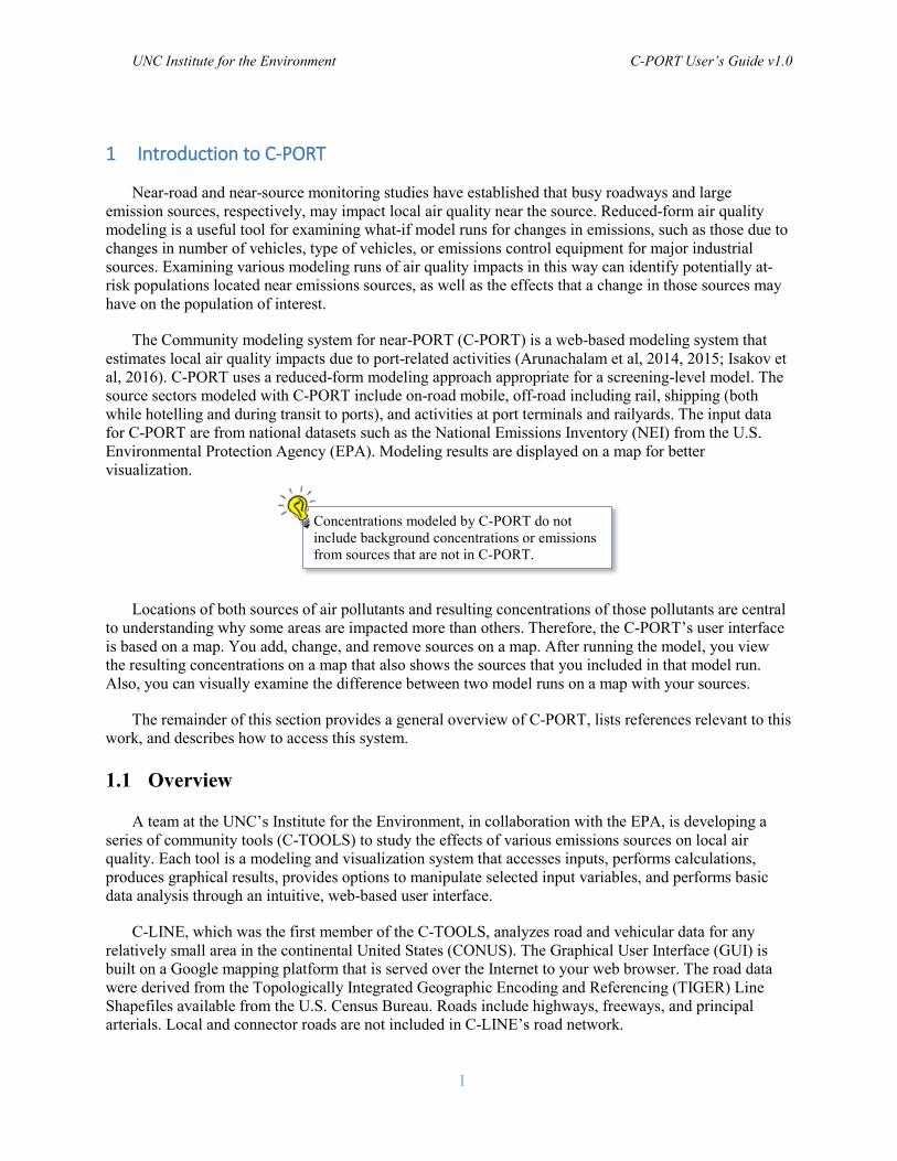
The Community modeling system for near-PORT (C-PORT) is a web-based modeling system that estimates local air quality impacts due to port-related activities (Arunachalam et al, 2014, 2015; Isakov et al, 2016). C-PORT uses a reduced-form modeling approach appropriate for a screening-level model. The source sectors modeled with C-PORT include on-road mobile, off-road including rail, shipping (both while hotelling and during transit to ports), and activities at port terminals and railyards. The input data for C-PORT are from national datasets such as the National Emissions Inventory (NEI) from the U.S. Environmental Protection Agency (EPA). Modeling results are displayed on a map for better visualization.
Locations of both sources of air pollutants and resulting concentrations of those pollutants are central to understanding why some areas are impacted more than others. Therefore, the C-PORT’s user interface is based on a map. You add, change, and remove sources on a map. After running the model, you view the resulting concentrations on a map that also shows the sources that you included in that model run. Also, you can visually examine the difference between two model runs on a map with your sources.
The remainder of this section provides a general overview of C-PORT, lists references relevant to this work, and describes how to access this system.
1.1 Overview
A team at the UNC’s Institute for the Environment, in collaboration with the EPA, is developing a series of community tools (C-TOOLS) to study the effects of various emissions sources on local air quality. Each tool is a modeling and visualization system that accesses inputs, performs calculations, produces graphical results, provides options to manipulate selected input variables, and performs basic data analysis through an intuitive, web-based user interface.
C-LINE, which was the first member of the C-TOOLS, analyzes road and vehicular data for any relatively small area in the continental United States (CONUS). The Graphical User Interface (GUI) is built on a Google mapping platform that is served over the Internet to your web browser. The road data were derived from the Topologically Integrated Geographic Encoding and Referencing (TIGER) Line Shapefiles available from the U.S. Census Bureau. Roads include highways, freeways, and principal arterials. Local and connector roads are not included in C-LINE’s road network.
Concentrations modeled by C-PORT do not include background concentrations or emissions from sources that are not in C-PORT.
UNC Institute for the Environment C-PORT User’s Guide v1.0
2
C-PORT is an expansion of C-LINE. Where C-LINE models roads and vehicles operating on those roads, C-PORT includes other types of vehicles and activities that occur at an ocean port. These include locomotives on rail lines and at railyards and ships traveling in shipping lanes and hotelling at docks. Other port activities are also modeled, including major industrial sources at docks and cargo transfers between ships and ground transportation. See Section 3 for additional information on data sources used in C-PORT.
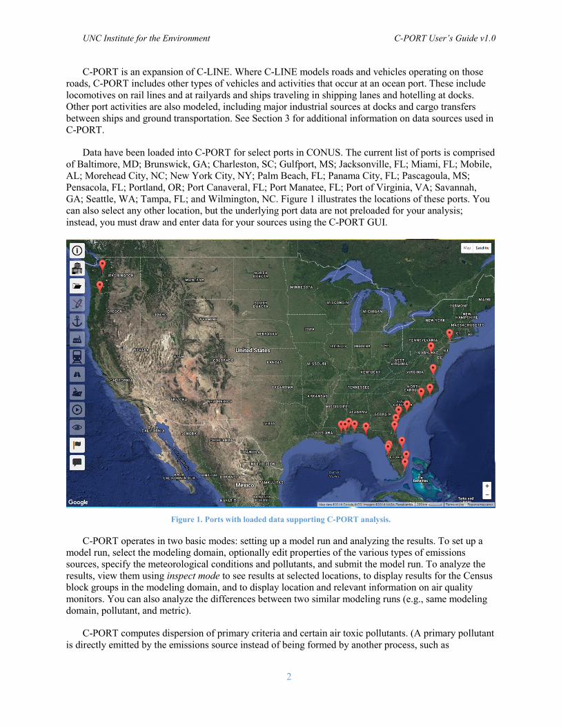
Data have been loaded into C-PORT for select ports in CONUS. The current list of ports is comprised of Baltimore, MD; Brunswick, GA; Charleston, SC; Gulfport, MS; Jacksonville, FL; Miami, FL; Mobile, AL; Morehead City, NC; New York City, NY; Palm Beach, FL; Panama City, FL; Pascagoula, MS; Pensacola, FL; Portland, OR; Port Canaveral, FL; Port Manatee, FL; Port of Virginia, VA; Savannah, GA; Seattle, WA; Tampa, FL; and Wilmington, NC. Figure 1 illustrates the locations of these ports. You can also select any other location, but the underlying port data are not preloaded for your analysis; instead, you must draw and enter data for your sources using the C-PORT GUI.
Figure 1. Ports with loaded data supporting C-PORT analysis.
C-PORT operates in two basic modes: setting up a model run and analyzing the results. To set up a model run, select the modeling domain, optionally edit properties of the various types of emissions sources, specify the meteorological conditions and pollutants, and submit the model run. To analyze the results, view them using inspect mode to see results at selected locations, to display results for the Census block groups in the modeling domain, and to display location and relevant information on air quality monitors. You can also analyze the differences between two similar modeling runs (e.g., same modeling domain, pollutant, and metric).
C-PORT computes dispersion of primary criteria and certain air toxic pollutants. (A primary pollutant is directly emitted by the emissions source instead of being formed by another process, such as
UNC Institute for the Environment C-PORT User’s Guide v1.0
3
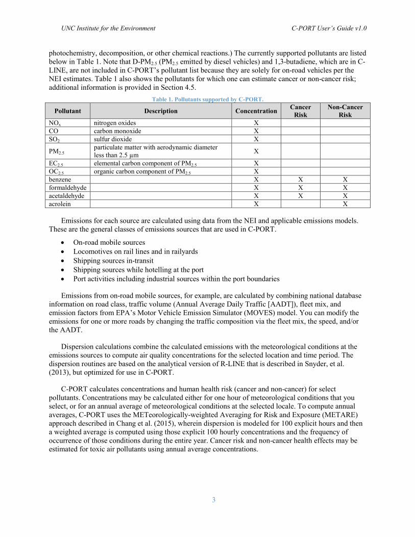
photochemistry, decomposition, or other chemical reactions.) The currently supported pollutants are listed below in Table 1. Note that D-PM2.5 (PM2.5 emitted by diesel vehicles) and 1,3-butadiene, which are in C-LINE, are not included in C-PORT’s pollutant list because they are solely for on-road vehicles per the NEI estimates. Table 1 also shows the pollutants for which one can estimate cancer or non-cancer risk; additional information is provided in Section 4.5.
Table 1. Pollutants supported by C-PORT.
Pollutant Description Concentration Cancer Risk
Non-Cancer Risk
NOx nitrogen oxides X CO carbon monoxide X SO2 sulfur dioxide X
PM2.5 particulate matter with aerodynamic diameter less than 2.5 µm X
EC2.5 elemental carbon component of PM2.5 X OC2.5 organic carbon component of PM2.5 X benzene X X X formaldehyde X X X acetaldehyde X X X acrolein X X
Emissions for each source are calculated using data from the NEI and applicable emissions models. These are the general classes of emissions sources that are used in C-PORT.
• On-road mobile sources • Locomotives on rail lines and in railyards • Shipping sources in-transit • Shipping sources while hotelling at the port • Port activities including industrial sources within the port boundaries
Emissions from on-road mobile sources, for example, are calculated by combining national database information on road class, traffic volume (Annual Average Daily Traffic [AADT]), fleet mix, and emission factors from EPA’s Motor Vehicle Emission Simulator (MOVES) model. You can modify the emissions for one or more roads by changing the traffic composition via the fleet mix, the speed, and/or the AADT.
Dispersion calculations combine the calculated emissions with the meteorological conditions at the emissions sources to compute air quality concentrations for the selected location and time period. The dispersion routines are based on the analytical version of R-LINE that is described in Snyder, et al. (2013), but optimized for use in C-PORT.
C-PORT calculates concentrations and human health risk (cancer and non-cancer) for select pollutants. Concentrations may be calculated either for one hour of meteorological conditions that you select, or for an annual average of meteorological conditions at the selected locale. To compute annual averages, C-PORT uses the METeorologically-weighted Averaging for Risk and Exposure (METARE) approach described in Chang et al. (2015), wherein dispersion is modeled for 100 explicit hours and then a weighted average is computed using those explicit 100 hourly concentrations and the frequency of occurrence of those conditions during the entire year. Cancer risk and non-cancer health effects may be estimated for toxic air pollutants using annual average concentrations.
UNC Institute for the Environment C-PORT User’s Guide v1.0
4
1.2 References
Arunachalam, S., T. Barzyk, V. Isakov, A. Venkatram, M. Snyder, N. A. Rice, B. Naess and K. Talgo (2014). C-PORT: A Community - scale Near - Source Air Quality System to Assess Port - related Air Quality Impacts, In Proceedings of the 16th International Conference on Harmonisation within Atmospheric Dispersion Modelling for Regulatory Purposes, September 2014, Varna, Bulgaria.
Arunachalam, S., H. Brantley, T. Barzyk, G. Hagler, V. Isakov, S. Kimbrough, B. Naess, N. Rice, M. Snyder, K. Talgo, A. Venkatram (2015). Assessment of Port-Related Air Quality Impacts: Geographic Analysis of Population, Int. J. Environ. Poll., 58(4):231-250.
Barzyk, Timothy M., Vlad Isakov, Saravanan Arunachalam, Akula Venkatram, Rich Cook, and Brian Naess (2015). A near-road modeling system for community-scale assessments of traffic-related air pollution in the United States. Environmental Modelling & Software 66: 46-56.
Chang, S.-Y. , W. Vizuete, A. Valencia, B. Naess, V. Isakov, T. Palma, M. Breen, S. Arunachalam (2015). A Modeling Framework for Characterizing Near-Road Air Pollutant Concentration at Community Scales, Sci. Total Environ. 538:905-921.
Isakov, V., Barzyk, T., Arunachalam, S., Snyder, M. & Venkatram, A. (2016). A Community-Scale Modeling System to Assess Port-Related Air Quality Impacts. Air Pollution Modeling and its Application XXIV, , Air Pollution Modeling and its Application XXIV, D.G. Steyn and N Chaumerliac (eds.), ISBN: 978-3-319-24478-5 (Online), Springer Proceedings in Complexity, pp. 385 -390.
Snyder, Michelle G., Akula Venkatram, David K. Heist, Steven G. Perry, William B. Petersen, and Vlad Isakov (2013). RLINE: A line source dispersion model for near-surface releases. Atmospheric Environment 77: 748-756.
1.3 Access to C-PORT
Access to C-PORT is granted to registered users of the CMAS Center. Go to the CMAS home page (https://www.cmascenter.org/) from a web browser and click “Log In” under the CMAS logo to navigate to the CMAS login page (see Figure 2). If you are a registered user, enter your email address and password and then press the Submit button. If you do not have a CMAS account, click the Create One link within the login message. This link takes you to the Create a CMAS Account page at https://www.cmascenter.org/register/create_account.cfm. Fill in the form and then mark your preferences at the bottom. When finished, click the Create Account button.
Figure 2. Log In to CMAS located on right side of header.
Once you have logged in to the CMAS Center, scroll down the page and look for the frame of “Supported Products” on the CMAS home page. Click the tab for “C-TOOLS” and then the “C-PORT”
UNC Institute for the Environment C-PORT User’s Guide v1.0
5
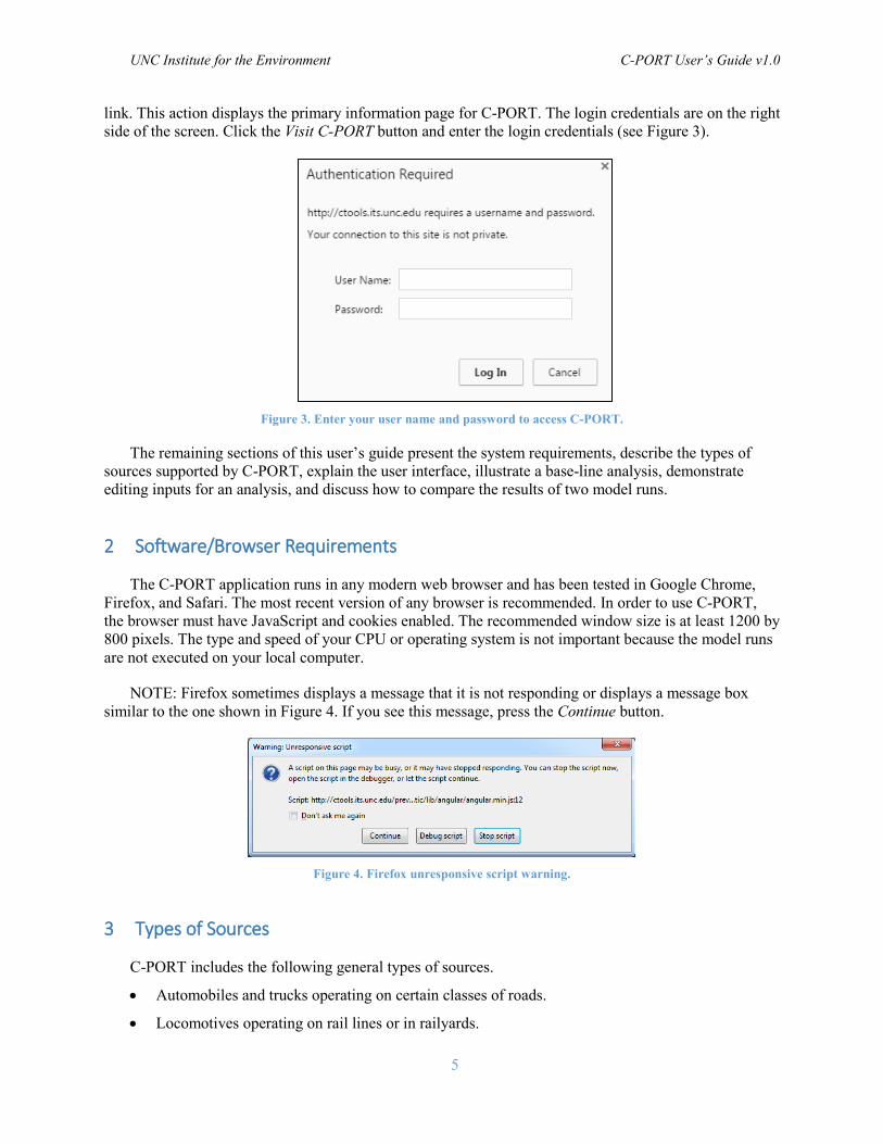
link. This action displays the primary information page for C-PORT. The login credentials are on the right side of the screen. Click the Visit C-PORT button and enter the login credentials (see Figure 3).
Figure 3. Enter your user name and password to access C-PORT.
The remaining sections of this user’s guide present the system requirements, describe the types of sources supported by C-PORT, explain the user interface, illustrate a base-line analysis, demonstrate editing inputs for an analysis, and discuss how to compare the results of two model runs.
2 Software/Browser Requirements
The C-PORT application runs in any modern web browser and has been tested in Google Chrome, Firefox, and Safari. The most recent version of any browser is recommended. In order to use C-PORT, the browser must have JavaScript and cookies enabled. The recommended window size is at least 1200 by 800 pixels. The type and speed of your CPU or operating system is not important because the model runs are not executed on your local computer.
NOTE: Firefox sometimes displays a message that it is not responding or displays a message box similar to the one shown in Figure 4. If you see this message, press the Continue button.
Figure 4. Firefox unresponsive script warning.
3 Types of Sources
C-PORT includes the following general types of sources.
• Automobiles and trucks operating on certain classes of roads.
• Locomotives operating on rail lines or in railyards.
UNC Institute for the Environment C-PORT User’s Guide v1.0
6
• Ships operating in shipping lanes outside the coastline or along inland waterways to gain access to terminals.
• Activities occurring within the boundaries of a terminal. These activities include hotelling (docked) ships that are producing emissions, ground-based activities such as transferring cargo between transportation modes (e.g., ship-to-truck), and other miscellaneous sources.
The remainder of this chapter discusses the types of emissions originating with each of these source types. The final section in this chapter provides a general overview of how the various emissions sources are classified for dispersion modeling.
3.1 Vehicles on Roads
Many types of vehicles operate on roads; these are called on-road mobile sources (ORM). C-PORT incorporates the paradigm and vehicle types of C-LINE. Four types of vehicles are included – automobiles and trucks that burn either gasoline or diesel fuel. Special vehicle types (e.g., electric vehicles and those that burn an alternative fuel) should be omitted from the AADT. Other diesel-burning vehicles including dump trucks, trash trucks, and buses should be included in the trucks burning diesel fuel.
The road data (i.e., line segments that define a road) are derived from the TIGER/Line Shapefiles available from the U.S. Census Bureau (https://www.census.gov/geo/maps-data/data/tiger.html). This dataset was filtered to include only highways, freeways, and principal arterials. Local and connector roads are not included in the road network.
Note that you cannot enter emissions from automobiles and trucks directly into C-PORT. Vehicular emissions are a function of many factors including speed, diurnal temperature range, engine load, age distribution of vehicles, and types of vehicles. These and other factors are input to the MOVES-2010b vehicle emissions model to calculate emission factors. To reduce execution time required for a C-PORT simulation, the MOVES model was previously executed for a wide range of conditions; its outputs in the form of emissions factors are available as supporting tables for C-PORT’s calculations.
3.2 Locomotives on Rails
EPA’s NEI-2011v1 emissions inventory was the starting point for rail emissions. C-PORT includes emissions for Class I diesel line haul locomotives. The activity and emissions factor data were processed through the Sparse Matrix Operator Kernel Emissions (SMOKE) modeling system to obtain the annual emissions in tons/yr for all pollutants included in C-PORT. Therefore, activity data and emissions factors are not available for these emissions categories.
3.2.1 Rail Lines
The location of rail lines was obtained from TIGER rail data (2010). Emissions (tons/yr) were apportioned to each rail segment based on the length of that segment, divided by the total length of rail line in that county. That is, the same rail traffic density is assumed to be present on each mile of rail in a county. If you add a new rail line, you must assign its emissions in tons/yr for that rail segment and not in some other units, such as tons/mi/yr.
UNC Institute for the Environment C-PORT User’s Guide v1.0
7
3.2.2 Railyards
Railyards were manually delineated in a GIS. First, the NEI was queried to obtain any data records providing a point location for yard locomotives. These points were then used to locate railyards, and polygons were drawn to delineate each railyard based on a satellite view in the GIS. If there were emissions for yard locomotives in a county associated with a port, but no location was included in the NEI, then the satellite view in the GIS was visually searched to locate one or more railyards.
NEI emissions from yard locomotives were assigned to railyards in the county in which the emissions occurred. If there were more than one railyard in a county and they did not have associated locations in the NEI, then emissions were apportioned among those railyards based on relative area.
3.3 Ships-in-Transit
C-PORT includes emissions for Class III commercial marine vessels (CMVs), which are sometimes referred to as Ocean Going Vessels (OGVs) in the literature, and Classes I and II smaller/recreational marine vessels. Channel data were extracted from the National Waterway Network (NWN) developed by the Oak Ridge National Laboratory (ORNL) and Vanderbilt University with input from the National Waterway GIS Design Committee (NWGISDC), whose members include the U.S. Army Corps of Engineers, Bureau of Transportation Statistics, and other federal agencies. The NWN is a geographic database of navigable waterways in and around the United States for analytical studies of waterway performance, for compiling commodity flow statistics, and for mapping purposes. For further information see http://www.navigationdatacenter.us/data/datanwn.htm.
The emissions for ships-in-transit are provided in tons/yr for each channel segment. Unlike ORM emissions, and like rail emissions, ships-in-transit do not have an activity level and an emissions factor.
3.3.1 Commercial Marine Vessels
Channels for Class III commercial marine vessels were obtained by merging the NWN with the Waterway Network Link Commodity Data (WNLCD; http://www.navigationdatacenter.us/data/datalink.htm) to determine channels with shipping activity. These channels were then delineated in a GIS as a series of straight lines from either the open ocean directly to a port or via a navigable, inland waterway upstream from an estuary or mouth of a river to a port. Applicable emissions from the NEI were then assigned to the delineated channels in tons/yr.
3.3.2 Smaller Marine Vessels
The Class I and II marine vessels were also routed based on the NWN, but without the merge with the WNLCD. This second dataset was not used because it is based on freight and many of these smaller ships are commercial fishing vessels. The relevant emissions were then apportioned to the channel segments based upon the fractional length of all channel segments assigned to the overall port.
3.4 Port Activities
Many types of activities take place within the port boundaries and at adjacent docks. Depending upon the importance or relative magnitude of emissions from those activities, you may want to model them individually or group them by type. For example, a coal-fired boiler is usually modeled as an individual source, but many small sources (e.g., mobile diesel ground vehicles) may be grouped together and modeled as a single area source.
UNC Institute for the Environment C-PORT User’s Guide v1.0
8
3.4.1 Hotelling Ships
Hotelling ships are large, commercial ships that are stopped at a pier/wharf/dock (PWD) or at anchorage close to the port. Depending upon regulations associated with a port, hotelling ships may run their auxiliary engines to provide power to support ship activities and cargo handlers or may use shore power (i.e., cold ironing). Only those ships using their engines should be designated as hotelling ships.
C-PORT marks locations where hotelling ships are generally located throughout the year. The sum of emissions for all ships located at one point over a time-span of one year is used to represent that source location. Also, a set of stack parameters that reasonably characterize the ships at that location is used to represent all ships. If you have two types of ships that use the same location for hotelling, you can model each of those types as a single source, but be certain to allocate the emissions from each of those types to its representative source. Be careful to not double-count emissions.
When computing emissions for hotelling ships, refer to governing regulations concerning the type of fuel to be used in port. Some locations may require low-sulfur or ultra-low-sulfur diesel fuel and/or biodiesel blends. The emissions from these fuels are different than those from typical diesel fuel.
3.4.2 Ground-based Activities on Terminals
A myriad of small sources operate through a terminal on unknown paths or large areas of pavement. Some examples are semi-trucks that pick up or drop off containers, gantry cranes, yard hostlers, and top picks.
3.4.3 Industrial Sources within Terminal
Depending upon location, a port may have a wide variety of industrial sources including an electricity generating unit (EGU), chemical plant, or refinery. Each of these industrial sources may have one or more emissions sources. If there are stacks or other types of hot or elevated sources, enter their information as a point source. If the source is at ground-level or consists of many similar small sources, combine them into one or more area sources. Additional information about each of these types of emissions sources is included in the following section.
3.5 Grouping Similar Sources
The previous parts of this section provided examples of types of sources as they exist in the physical world. This section groups these sources into four types based on how dispersion is modeled through the air. These four types are line sources, buoyant line sources, area sources, and point sources. Each of these is discussed with examples in this section.
3.5.1 Line Sources
A line source is a source of emissions to the atmosphere, where the emissions are released uniformly along a straight line. Based upon the type of source, an initial lateral spread (i.e., distance orthogonal to the line) and an initial vertical spread (i.e., vertical thickness of the source) are used. These factors take into account the width of the roadway and the average source height of the emissions source from the vehicles.
Two types of line sources in C-PORT are roads and rail lines. In the case of roads, the emissions sources are vehicles that may be moving or temporarily stopped (e.g., at a red stop light). But, the only
UNC Institute for the Environment C-PORT User’s Guide v1.0
9
known pieces of information made available to the user are the overall mix of vehicles by type (i.e., fleet), the number of vehicles, and the speed of the vehicles. Other statistical measures, such as the age distribution of the vehicles, load on the engine, and types of emissions controls, are determined within C-PORT and the underlying MOVES emissions model.
The other type of line source in C-PORT is the rail line on which locomotives produce emissions. The type of locomotives, load based on tonnage being pulled and grade, and hour of the year during which a locomotive travels on a specific straight segment of track are not known. Therefore, the total emissions that are provided in the NEI based on a county are allocated by mile of track within the county. For example, if a segment of track is one mile long and there are 100 miles of track in a county, then 1/100 or 0.01 of the total locomotive emissions in the county are allocated to that one-track segment in tons/yr.
3.5.2 Buoyant Line Sources
A buoyant line source is a line source that has sufficient heat or upward exit velocity where the emissions are exiting the source to cause the emissions to rise. This type of source is handled like a line source with the buoyancy of a hot point source. In C-PORT, the ships-in-transit source type is modeled as a buoyant line source.
3.5.3 Area Sources
An area source belongs to a relatively minor category of emissions sources, where the locations are either unknown or too numerous to handle as individual sources. C-PORT has two types of area sources: yard locomotives in railyards and terminal-related activities.
When a county has more than one railyard, the locomotive emissions for the county are apportioned to each railyard based on its relative size. For a specific railyard, the emissions are uniformly spread throughout the railyard polygon and are dispersed from there.
Terminal-related activities are handled like those in railyards, but are placed on the terminal’s polygon.
3.5.4 Point sources
A point source is typically a large, stationary emissions source with a known location. In C-PORT the point sources usually reside within the boundary of a terminal’s polygon. Similar to sources other than ORM, emissions are specified in tons/yr for each pollutant. However, a point source may also have an elevated outlet for the emissions (e.g., a stack) and the emissions may be hot compared to the ambient air. The emissions may also be forced from the outlet due to the heat or a blower.
Therefore, both the emissions (tons/yr) and stack parameters must be defined for each point source. The stack parameters are the stack height (m), inner stack diameter at the top (m), exit temperature (°K), and exit velocity (m/s).
4 User Interface
This section describes how to navigate the screens of C-PORT. First, we describe the overall screen layout and then the meaning of the navigation tiles and how to use them. Then, we provide an overview of performing an analysis, viewing each type of results, and displaying ambient air quality data from AQS monitors.
UNC Institute for the Environment C-PORT User’s Guide v1.0
10
4.1 Overall Screen Layout
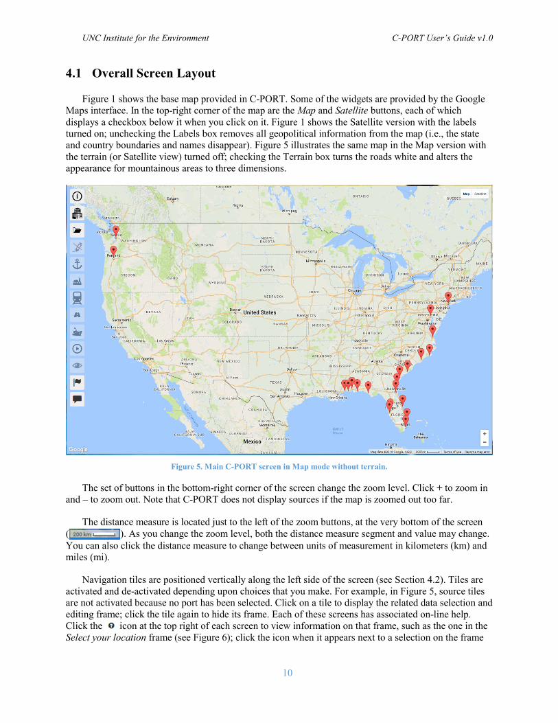
Figure 1 shows the base map provided in C-PORT. Some of the widgets are provided by the Google Maps interface. In the top-right corner of the map are the Map and Satellite buttons, each of which displays a checkbox below it when you click on it. Figure 1 shows the Satellite version with the labels turned on; unchecking the Labels box removes all geopolitical information from the map (i.e., the state and country boundaries and names disappear). Figure 5 illustrates the same map in the Map version with the terrain (or Satellite view) turned off; checking the Terrain box turns the roads white and alters the appearance for mountainous areas to three dimensions.
Figure 5. Main C-PORT screen in Map mode without terrain.
The set of buttons in the bottom-right corner of the screen change the zoom level. Click + to zoom in and – to zoom out. Note that C-PORT does not display sources if the map is zoomed out too far.
The distance measure is located just to the left of the zoom buttons, at the very bottom of the screen ( ). As you change the zoom level, both the distance measure segment and value may change. You can also click the distance measure to change between units of measurement in kilometers (km) and miles (mi).
Navigation tiles are positioned vertically along the left side of the screen (see Section 4.2). Tiles are activated and de-activated depending upon choices that you make. For example, in Figure 5, source tiles are not activated because no port has been selected. Click on a tile to display the related data selection and editing frame; click the tile again to hide its frame. Each of these screens has associated on-line help. Click the icon at the top right of each screen to view information on that frame, such as the one in the Select your location frame (see Figure 6); click the icon when it appears next to a selection on the frame
UNC Institute for the Environment C-PORT User’s Guide v1.0
11
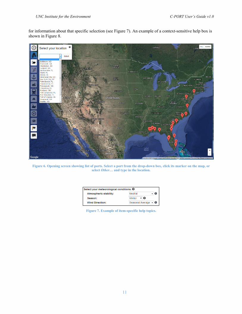
for information about that specific selection (see Figure 7). An example of a context-sensitive help box is shown in Figure 8.
Figure 7. Example of item-specific help topics.
Figure 6. Opening screen showing list of ports. Select a port from the drop-down box, click its marker on the map, or select Other… and type in the location.
UNC Institute for the Environment C-PORT User’s Guide v1.0
12
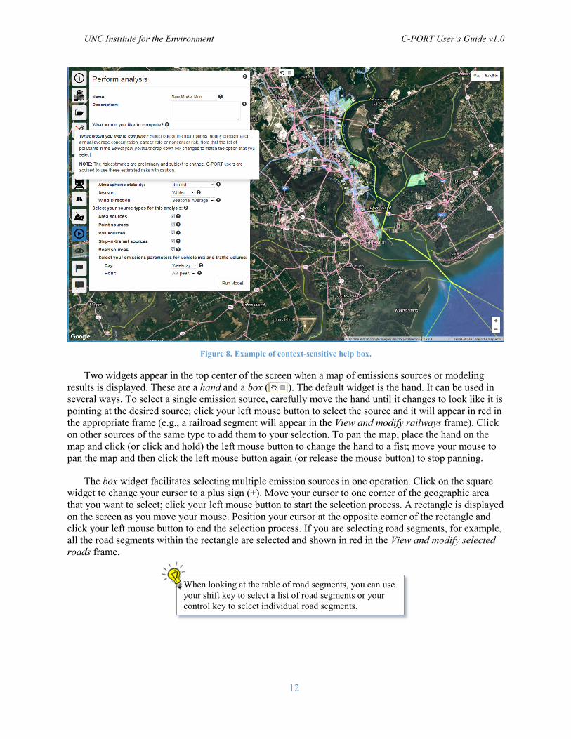
Figure 8. Example of context-sensitive help box.
Two widgets appear in the top center of the screen when a map of emissions sources or modeling results is displayed. These are a hand and a box ( ). The default widget is the hand. It can be used in several ways. To select a single emission source, carefully move the hand until it changes to look like it is pointing at the desired source; click your left mouse button to select the source and it will appear in red in the appropriate frame (e.g., a railroad segment will appear in the View and modify railways frame). Click on other sources of the same type to add them to your selection. To pan the map, place the hand on the map and click (or click and hold) the left mouse button to change the hand to a fist; move your mouse to pan the map and then click the left mouse button again (or release the mouse button) to stop panning.
The box widget facilitates selecting multiple emission sources in one operation. Click on the square widget to change your cursor to a plus sign (+). Move your cursor to one corner of the geographic area that you want to select; click your left mouse button to start the selection process. A rectangle is displayed on the screen as you move your mouse. Position your cursor at the opposite corner of the rectangle and click your left mouse button to end the selection process. If you are selecting road segments, for example, all the road segments within the rectangle are selected and shown in red in the View and modify selected roads frame.
When looking at the table of road segments, you can use your shift key to select a list of road segments or your control key to select individual road segments.
UNC Institute for the Environment C-PORT User’s Guide v1.0
13
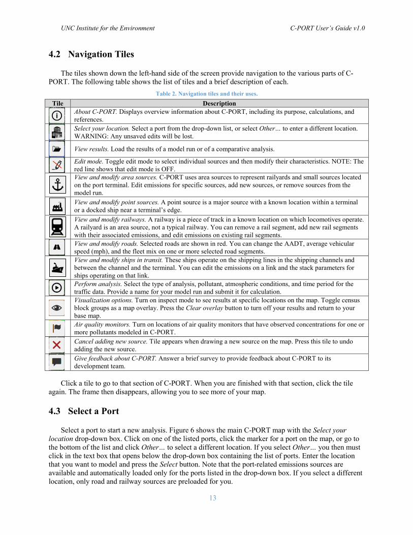
4.2 Navigation Tiles
The tiles shown down the left-hand side of the screen provide navigation to the various parts of C-PORT. The following table shows the list of tiles and a brief description of each.
Table 2. Navigation tiles and their uses. Tile Description
About C-PORT. Displays overview information about C-PORT, including its purpose, calculations, and references.
Select your location. Select a port from the drop-down list, or select Other… to enter a different location. WARNING: Any unsaved edits will be lost.
View results. Load the results of a model run or of a comparative analysis.
Edit mode. Toggle edit mode to select individual sources and then modify their characteristics. NOTE: The red line shows that edit mode is OFF.
View and modify area sources. C-PORT uses area sources to represent railyards and small sources located on the port terminal. Edit emissions for specific sources, add new sources, or remove sources from the model run.
View and modify point sources. A point source is a major source with a known location within a terminal or a docked ship near a terminal’s edge.
View and modify railways. A railway is a piece of track in a known location on which locomotives operate. A railyard is an area source, not a typical railway. You can remove a rail segment, add new rail segments with their associated emissions, and edit emissions on existing rail segments.
View and modify roads. Selected roads are shown in red. You can change the AADT, average vehicular speed (mph), and the fleet mix on one or more selected road segments.
View and modify ships in transit. These ships operate on the shipping lines in the shipping channels and between the channel and the terminal. You can edit the emissions on a link and the stack parameters for ships operating on that link.
Perform analysis. Select the type of analysis, pollutant, atmospheric conditions, and time period for the traffic data. Provide a name for your model run and submit it for calculation.
Visualization options. Turn on inspect mode to see results at specific locations on the map. Toggle census block groups as a map overlay. Press the Clear overlay button to turn off your results and return to your base map.
Air quality monitors. Turn on locations of air quality monitors that have observed concentrations for one or more pollutants modeled in C-PORT.
Cancel adding new source. Tile appears when drawing a new source on the map. Press this tile to undo adding the new source.
Give feedback about C-PORT. Answer a brief survey to provide feedback about C-PORT to its development team.
Click a tile to go to that section of C-PORT. When you are finished with that section, click the tile again. The frame then disappears, allowing you to see more of your map.
4.3 Select a Port
Select a port to start a new analysis. Figure 6 shows the main C-PORT map with the Select your location drop-down box. Click on one of the listed ports, click the marker for a port on the map, or go to the bottom of the list and click Other… to select a different location. If you select Other… you then must click in the text box that opens below the drop-down box containing the list of ports. Enter the location that you want to model and press the Select button. Note that the port-related emissions sources are available and automatically loaded only for the ports listed in the drop-down box. If you select a different location, only road and railway sources are preloaded for you.
UNC Institute for the Environment C-PORT User’s Guide v1.0
14
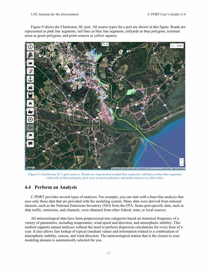
Figure 9 shows the Charleston, SC port. All source types for a port are shown in this figure. Roads are represented as pink line segments, rail lines as blue line segments, railyards as blue polygons, terminal areas as green polygons, and point sources as yellow squares.
Figure 9. Charleston, SC's port sources. Roads are represented as pink line segments, rail lines as blue line segments,
railyards as blue polygons, port area as green polygons, and point sources as yellow dots.
4.4 Perform an Analysis
C-PORT provides several types of analyses. For example, you can start with a base-line analysis that uses only those data that are provided with the modeling system. Many data were derived from national datasets, such as the National Emissions Inventory (NEI) from the EPA. Some port-specific data, such as ship traffic, emissions, and channels, were obtained from other federal, state, or local sources.
All meteorological data have been preprocessed into categories based on statistical frequency of a variety of parameters, including temperature, wind speed and direction, and atmospheric stability. This method supports annual analyses without the need to perform dispersion calculations for every hour of a year. It also allows fast lookup of typical (median) values and information related to a combination of atmospheric stability, season, and wind direction. The meteorological station that is the closest to your modeling domain is automatically selected for you.
UNC Institute for the Environment C-PORT User’s Guide v1.0
15
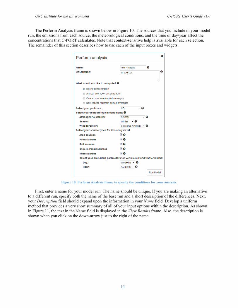
The Perform Analysis frame is shown below in Figure 10. The sources that you include in your model run, the emissions from each source, the meteorological conditions, and the time of day/year affect the concentrations that C-PORT calculates. Note that context-sensitive help is available for each selection. The remainder of this section describes how to use each of the input boxes and widgets.
Figure 10. Perform Analysis frame to specify the conditions for your analysis.
First, enter a name for your model run. The name should be unique. If you are making an alternative to a different run, specify both the name of the base run and a short description of the differences. Next, your Description field should expand upon the information in your Name field. Develop a uniform method that provides a very short summary of all of your input options within the description. As shown in Figure 11, the text in the Name field is displayed in the View Results frame. Also, the description is shown when you click on the down-arrow just to the right of the name.
UNC Institute for the Environment C-PORT User’s Guide v1.0
16
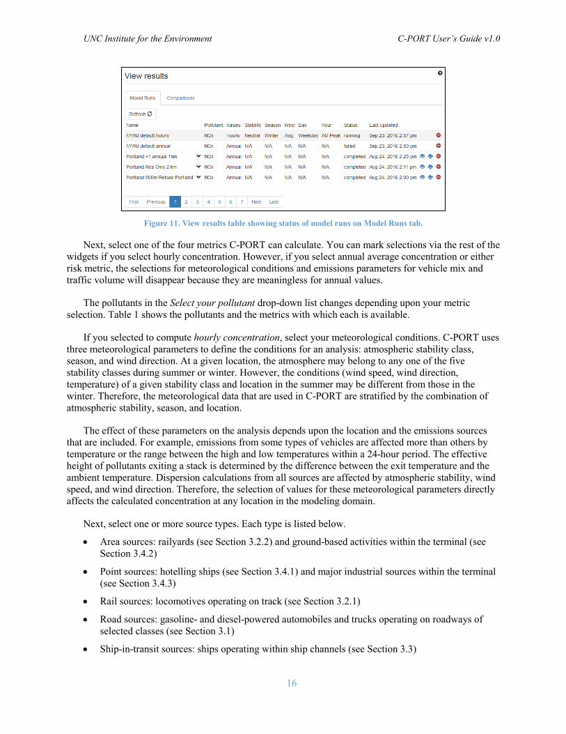
Figure 11. View results table showing status of model runs on Model Runs tab.
Next, select one of the four metrics C-PORT can calculate. You can mark selections via the rest of the widgets if you select hourly concentration. However, if you select annual average concentration or either risk metric, the selections for meteorological conditions and emissions parameters for vehicle mix and traffic volume will disappear because they are meaningless for annual values.
The pollutants in the Select your pollutant drop-down list changes depending upon your metric selection. Table 1 shows the pollutants and the metrics with which each is available.
If you selected to compute hourly concentration, select your meteorological conditions. C-PORT uses three meteorological parameters to define the conditions for an analysis: atmospheric stability class, season, and wind direction. At a given location, the atmosphere may belong to any one of the five stability classes during summer or winter. However, the conditions (wind speed, wind direction, temperature) of a given stability class and location in the summer may be different from those in the winter. Therefore, the meteorological data that are used in C-PORT are stratified by the combination of atmospheric stability, season, and location.
The effect of these parameters on the analysis depends upon the location and the emissions sources that are included. For example, emissions from some types of vehicles are affected more than others by temperature or the range between the high and low temperatures within a 24-hour period. The effective height of pollutants exiting a stack is determined by the difference between the exit temperature and the ambient temperature. Dispersion calculations from all sources are affected by atmospheric stability, wind speed, and wind direction. Therefore, the selection of values for these meteorological parameters directly affects the calculated concentration at any location in the modeling domain.
Next, select one or more source types. Each type is listed below.
• Area sources: railyards (see Section 3.2.2) and ground-based activities within the terminal (see Section 3.4.2)
• Point sources: hotelling ships (see Section 3.4.1) and major industrial sources within the terminal (see Section 3.4.3)
• Rail sources: locomotives operating on track (see Section 3.2.1)
• Road sources: gasoline- and diesel-powered automobiles and trucks operating on roadways of selected classes (see Section 3.1)
• Ship-in-transit sources: ships operating within ship channels (see Section 3.3)

UNC Institute for the Environment C-PORT User’s Guide v1.0
17
Finally, if you have checked the Road sources box and are computing Hourly concentration, you can select two emissions parameters for vehicle mix and traffic volume: Day and Hour. Use the drop-down box for Day to select either Weekday or Weekend. Then, select one of the four time periods under Hour:
• AM peak: the morning rush period (7:00am - 8:59am local time)
• Midday: the lower traffic volumes between the AM and PM rush periods (9:00am – 3:59pm local time)
• PM peak: the afternoon rush period (4:00pm - 6:59pm local time)
• Off-prime: time period before AM rush and after PM rush
• By adding and removing sources, moving sources, and changing the quantity of emissions in your analysis, you can perform a large variety of “what-if” scenarios. You can then run comparisons between any of these scenarios with your base-line scenario, or comparisons between two of these scenarios. Section 7 provides further information on running comparative analyses.
4.5 View Results
C-PORT shows your model results on a map. This presentation illustrates hot spots (i.e., localized areas of higher concentrations) and areas of lesser concern (i.e., lower concentrations). When you perform a comparative analysis by viewing the differences between the results of two scenarios, you can easily see where C-PORT predicts changes in concentrations or health effects from changes in emissions.
Select the View results tile to access your model results. Your results are separated into two tabs: Model Runs and Comparisons. An example of the Model Runs tab is shown above in Figure 11. Press the Refresh button to update your list of model runs and their current status. You can see that the model run that was submitted last is shown at the top of the list with the status “running”. The results from that model run are shown below (Figure 12). However, the status “failed” is shown for the model run “NY/NJ default annual”. If you have a model run that fails, please wait a few minutes and try it again. If it still fails, try zooming in for a smaller domain (fewer sources). If that still fails, please email us the information shown in your View results frame, using the Give feedback button on the left panel.
If you have a model run that fails, do NOT start or load a different scenario! Doing so will lose your model run entirely.
UNC Institute for the Environment C-PORT User’s Guide v1.0
18
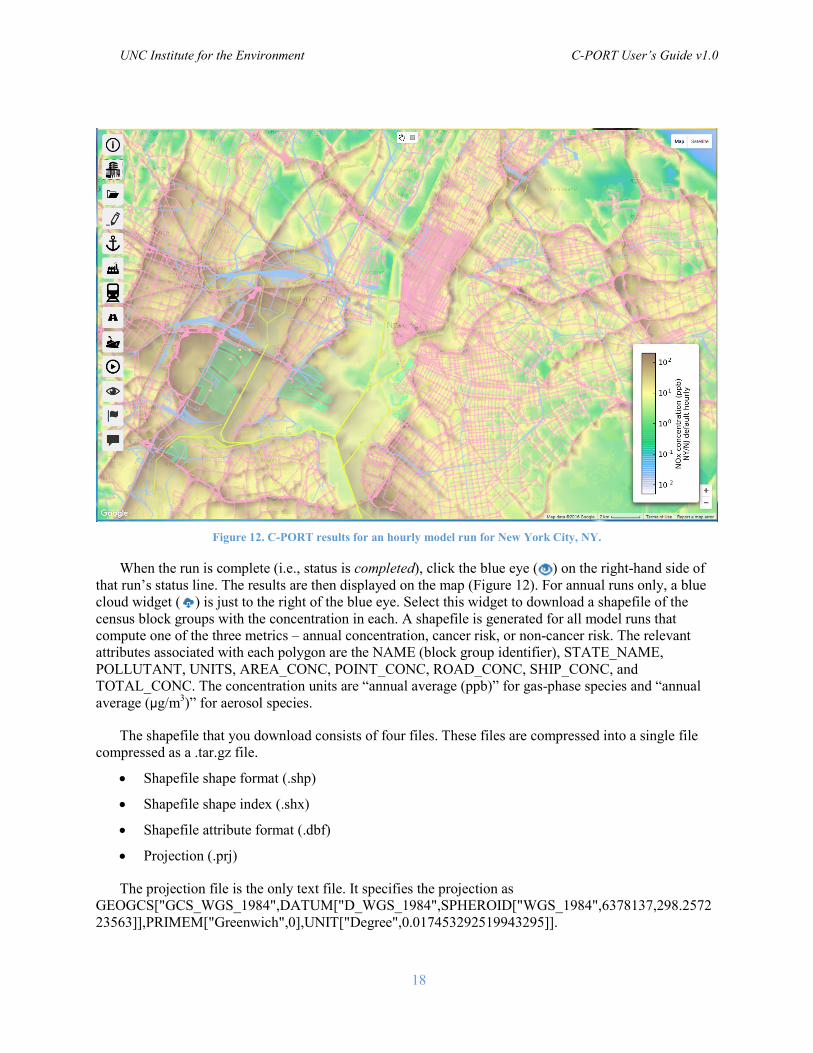
Figure 12. C-PORT results for an hourly model run for New York City, NY.
When the run is complete (i.e., status is completed), click the blue eye ( ) on the right-hand side of that run’s status line. The results are then displayed on the map (Figure 12). For annual runs only, a blue cloud widget ( ) is just to the right of the blue eye. Select this widget to download a shapefile of the census block groups with the concentration in each. A shapefile is generated for all model runs that compute one of the three metrics – annual concentration, cancer risk, or non-cancer risk. The relevant attributes associated with each polygon are the NAME (block group identifier), STATE_NAME, POLLUTANT, UNITS, AREA_CONC, POINT_CONC, ROAD_CONC, SHIP_CONC, and TOTAL_CONC. The concentration units are “annual average (ppb)” for gas-phase species and “annual average (μg/m3)” for aerosol species.
The shapefile that you download consists of four files. These files are compressed into a single file compressed as a .tar.gz file.
• Shapefile shape format (.shp)
• Shapefile shape index (.shx)
• Shapefile attribute format (.dbf)
• Projection (.prj)
The projection file is the only text file. It specifies the projection as GEOGCS["GCS_WGS_1984",DATUM["D_WGS_1984",SPHEROID["WGS_1984",6378137,298.257223563]],PRIMEM["Greenwich",0],UNIT["Degree",0.017453292519943295]].
UNC Institute for the Environment C-PORT User’s Guide v1.0
19
The results of the model run are displayed using a logarithmic scale. The legend in the lower right hand corner shows the color range for the minimum through maximum values calculated. For all model run types, the minimum value that can be displayed is 10-6. The actual minimum displayed depends upon the smallest values calculated in the model run.
Calculated values above pollutant-specific maximums are displayed in dark brown. The maximum value displayed depends upon the type of model run. For hourly and annual average model runs, a pollutant-specific maximum is used, based on ranges at or near the EPA’s National Ambient Air Quality Standard (NAAQS) for criteria pollutants, or the EPA’s Reference Concentration (RfC) for air toxics. Model runs that calculate cancer risk use a maximum value of 100 per million, while non-cancer risk has a maximum hazard quotient (HQ) of 1.
4.5.1 Visualization Options
When viewing the results of your analysis, click the Visualization options tile, which looks like a human eye ( ), to display the Visualization options frame (see Figure 13). You have three types of functionality on this frame: inspect mode, census block groups, and clear overlay.
Inspect mode displays the concentration at one or more selected locations on your map. To access this feature, click the Turn on inspect mode button. Your cursor then changes to a plus sign (+). You can then click on one or more locations of interest within your modeling domain. C-PORT displays the concentration and the coordinates of the location in (latitude, longitude) degrees, not (longitude, latitude).
NOTE: The concentration is not interpolated. Instead, it is obtained from the value of the nearest receptor point (i.e., nearest neighbor method). Also, if the bubble of information would extend beyond the edge of the visible map, C-PORT scrolls the map to make the entire bubble visible. Currently, there is no way to manually reposition a bubble, such as when one hides part of another bubble; you need to close the top bubble to see the information in the hidden bubble.
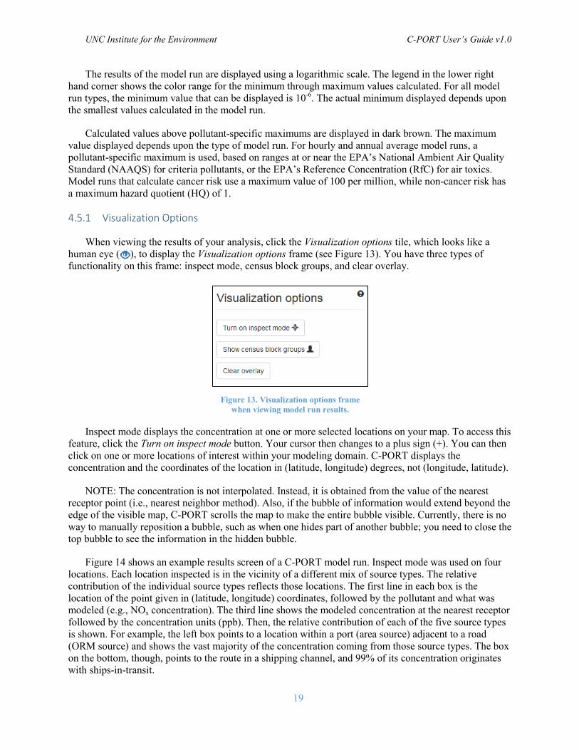
Figure 14 shows an example results screen of a C-PORT model run. Inspect mode was used on four locations. Each location inspected is in the vicinity of a different mix of source types. The relative contribution of the individual source types reflects those locations. The first line in each box is the location of the point given in (latitude, longitude) coordinates, followed by the pollutant and what was modeled (e.g., NOx concentration). The third line shows the modeled concentration at the nearest receptor followed by the concentration units (ppb). Then, the relative contribution of each of the five source types is shown. For example, the left box points to a location within a port (area source) adjacent to a road (ORM source) and shows the vast majority of the concentration coming from those source types. The box on the bottom, though, points to the route in a shipping channel, and 99% of its concentration originates with ships-in-transit.
Figure 13. Visualization options frame when viewing model run results.
UNC Institute for the Environment C-PORT User’s Guide v1.0
20
Figure 14. Inspect mode for annual concentration model run.
If you want to turn off one of the boxes, just click the X in its top right-hand corner. If you want to dismiss all of the boxes and end inspect mode, open the Visualization options frame again and click the Turn off inspect mode button, which is visible only when inspect mode is on.
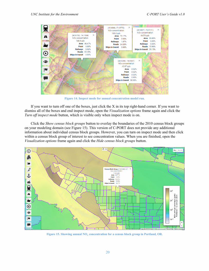
Click the Show census block groups button to overlay the boundaries of the 2010 census block groups on your modeling domain (see Figure 15). This version of C-PORT does not provide any additional information about individual census block groups. However, you can turn on inspect mode and then click within a census block group of interest to see concentration values. When you are finished, open the Visualization options frame again and click the Hide census block groups button.
Figure 15. Showing annual NOx concentration for a census block group in Portland, OR.
UNC Institute for the Environment C-PORT User’s Guide v1.0
21
When you are finished working with the results on your map, open the Visualization options frame and click the Clear overlay button. This removes the overlay of your modeling results, legend, values from inspect mode, and census block group boundaries. The Visualization options tile is also deactivated.
4.5.2 Concentrations
You can compute concentrations for your modeling domain as either 1-hr concentrations for specified meteorological conditions or an annual average. When viewing results of a model run, the same view is provided for both 1-hr and annual concentrations.
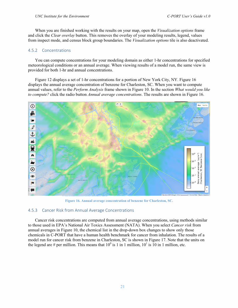
Figure 12 displays a set of 1-hr concentrations for a portion of New York City, NY. Figure 16 displays the annual average concentration of benzene for Charleston, SC. When you want to compute annual values, refer to the Perform Analysis frame shown in Figure 10. In the section What would you like to compute? click the radio button Annual average concentrations. The results are shown in Figure 16.
Figure 16. Annual average concentration of benzene for Charleston, SC.
4.5.3 Cancer Risk from Annual Average Concentrations
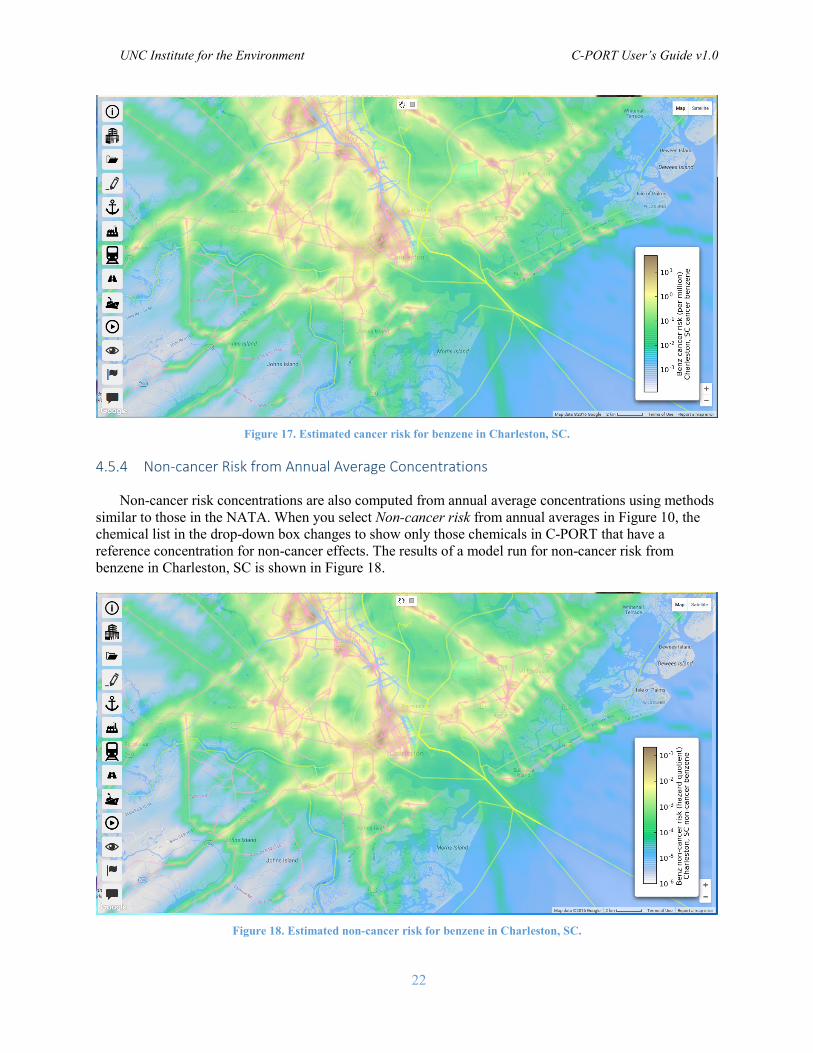
Cancer risk concentrations are computed from annual average concentrations, using methods similar to those used in EPA’s National Air Toxics Assessment (NATA). When you select Cancer risk from annual averages in Figure 10, the chemical list in the drop-down box changes to show only those chemicals in C-PORT that have a human health benchmark for cancer from inhalation. The results of a model run for cancer risk from benzene in Charleston, SC is shown in Figure 17. Note that the units on the legend are # per million. This means that 100 is 1 in 1 million, 101 is 10 in 1 million, etc.
UNC Institute for the Environment C-PORT User’s Guide v1.0
22
Figure 17. Estimated cancer risk for benzene in Charleston, SC.
4.5.4 Non-cancer Risk from Annual Average Concentrations
Non-cancer risk concentrations are also computed from annual average concentrations using methods similar to those in the NATA. When you select Non-cancer risk from annual averages in Figure 10, the chemical list in the drop-down box changes to show only those chemicals in C-PORT that have a reference concentration for non-cancer effects. The results of a model run for non-cancer risk from benzene in Charleston, SC is shown in Figure 18.
Figure 18. Estimated non-cancer risk for benzene in Charleston, SC.
UNC Institute for the Environment C-PORT User’s Guide v1.0
23
Note how the spatial patterns shown in Figure 16 through Figure 18 are identical. That is expected because all three of those figures are based on annual concentration, which is shown in Figure 16. The differences among the three figures are shown in the legend. Also, although the colors are the same, the range and breakpoints are different, with the maximum value on the legend of 100, 101, and 10-1 for concentration, cancer risk, and non-cancer risk, respectively.
4.6 View Air Quality Data
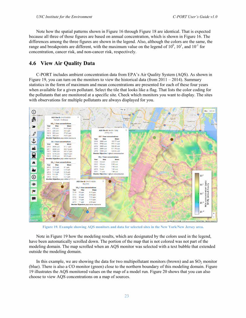
C-PORT includes ambient concentration data from EPA’s Air Quality System (AQS). As shown in Figure 19, you can turn on the monitors to view the historical data (from 2011 – 2014). Summary statistics in the form of maximum and mean concentrations are presented for each of these four years when available for a given pollutant. Select the tile that looks like a flag. That lists the color coding for the pollutants that are monitored at a specific site. Check which monitors you want to display. The sites with observations for multiple pollutants are always displayed for you.
Figure 19. Example showing AQS monitors and data for selected sites in the New York/New Jersey area.
Note in Figure 19 how the modeling results, which are designated by the colors used in the legend, have been automatically scrolled down. The portion of the map that is not colored was not part of the modeling domain. The map scrolled when an AQS monitor was selected with a text bubble that extended outside the modeling domain.
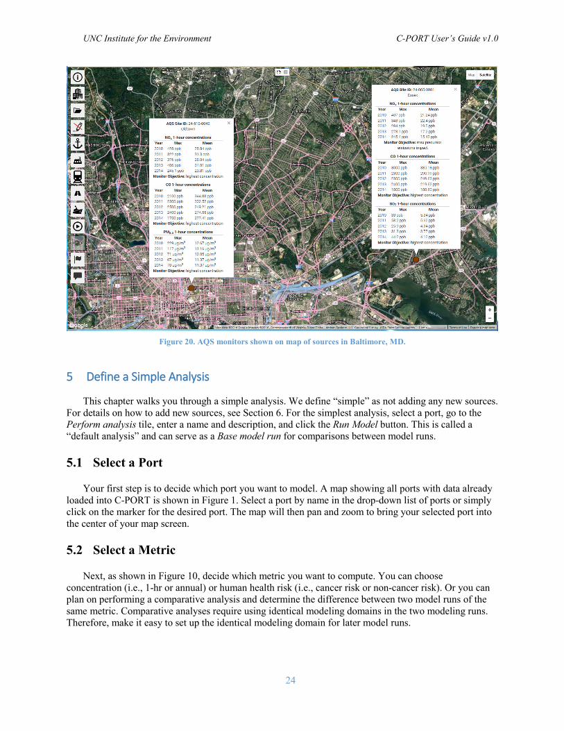
In this example, we are showing the data for two multipollutant monitors (brown) and an SO2 monitor (blue). There is also a CO monitor (green) close to the northern boundary of this modeling domain. Figure 19 illustrates the AQS monitored values on the map of a model run. Figure 20 shows that you can also choose to view AQS concentrations on a map of sources.
UNC Institute for the Environment C-PORT User’s Guide v1.0
24
Figure 20. AQS monitors shown on map of sources in Baltimore, MD.
5 Define a Simple Analysis
This chapter walks you through a simple analysis. We define “simple” as not adding any new sources. For details on how to add new sources, see Section 6. For the simplest analysis, select a port, go to the Perform analysis tile, enter a name and description, and click the Run Model button. This is called a “default analysis” and can serve as a Base model run for comparisons between model runs.
5.1 Select a Port
Your first step is to decide which port you want to model. A map showing all ports with data already loaded into C-PORT is shown in Figure 1. Select a port by name in the drop-down list of ports or simply click on the marker for the desired port. The map will then pan and zoom to bring your selected port into the center of your map screen.
5.2 Select a Metric
Next, as shown in Figure 10, decide which metric you want to compute. You can choose concentration (i.e., 1-hr or annual) or human health risk (i.e., cancer risk or non-cancer risk). Or you can plan on performing a comparative analysis and determine the difference between two model runs of the same metric. Comparative analyses require using identical modeling domains in the two modeling runs. Therefore, make it easy to set up the identical modeling domain for later model runs.
UNC Institute for the Environment C-PORT User’s Guide v1.0
25
Regardless of the type of analysis, pan and zoom the map and adjust the size of your browser window to arrive at the modeling domain you want. Your modeling domain is identified as the center of your map and the up-down and left-right extents of your browser window.
5.3 Select a Pollutant
The list of available pollutants changes to fit the metric that you choose. See Table 1 for the list of pollutants which are available for each metric. You can select only one pollutant for a model run.
5.4 Select Meteorological Conditions
You can select meteorological conditions only if you selected hourly concentrations for your metric. There are three categories of meteorological conditions that you need to select.
• Atmospheric stability: Stratified into five stability classes listed in order of increasing atmospheric turbulence
o Stable: Relatively stable atmosphere (lower dispersion rate) that produces greater ground-level concentrations near the emissions source and along the average wind direction.
o Slightly Stable: Atmosphere is still stable, but not as stable as the "stable" category.
o Neutral: Atmosphere is neither stable nor convective.
o Slightly Convective: Increased turbulence in the atmosphere tends to expand the pollution plume downwind, decreasing ground-level concentrations.
o Convective: Stability class with greatest turbulence that disperses the pollutants more quickly resulting in a wider, thicker plume with lower ground-level concentrations along the average wind direction.
• Season: Select either summer or winter conditions. The average temperature is lower in winter than in summer.
• Wind direction: Seasonal Average is the average wind direction corresponding to the season selected. Other selections are the 16 compass directions: South to North, SSW to NNE, SSE to NNW, etc.
5.5 Types of Sources to Include
You can select your source types as one or more of area, point, rail, ship-in-transit, and road sources. If you are planning to perform a comparative analysis, focus on the source types you intend to change. For example, you do not need to compute emissions and concentrations from sources on roads if your analysis is looking at the effects of increasing rail traffic. But, if you plan on performing model runs with all source types, then include them all in every model run.
5.6 Special Selections for Vehicles on Roads
If you are including Road Sources in this model run, you can also select values for two other parameters. These are used when running the model that computes emissions factors for the cars and trucks operating on roads.
UNC Institute for the Environment C-PORT User’s Guide v1.0
26
• Day: Select weekday or weekend to determine the hourly traffic patterns (number and types of vehicles) to be modeled.
• Hour: Select one of four possible time periods corresponding with traffic activity patterns.
o AM peak: The morning rush hour (7:00 – 8:59 A.M. local time)
o Midday: The lower traffic volume between the AM and PM rush periods (9:00 A.M. – 3:59 P.M.)
o PM peak: The afternoon rush period (4:00 – 6:59 P.M.)
o Off peak: Time period before AM peak and after PM peak
5.7 Run the Model
Click the Run Model button in the bottom, right-hand side of the Perform analysis frame. C-PORT automatically saves the selections and conditions that you designated for your model run when you click this button. This is your only opportunity to save your model.
C-PORT deactivates and animates the Run Model button while setting up the files for your model run. When the animation stops, C-PORT activates the button again. At this time you can activate the View results tile; press the Refresh button to show the status of your newest model run.
5.8 View Results
From View Results help:
This tile contains 2 tabs that are associated with saved model runs.
• Use the Model Runs tab to load a saved model run, to view the status of a submitted model run, and if completed, to view the results.
• Use the Comparisons tab to create a comparison between two model runs that have status "Completed", to view the status of a submitted comparison between two model runs, and if completed, to view the results.
If you are currently working on one of your model runs, it is shown in red. NOTE: If you select a different saved model run, any changes that you have made to your current model run and have not saved will be lost. If you have changes that you want to save, leave this tile, go to the Perform analysis tile, and enter a new model run name and description; press the Run Model button. Then, return to this tile and select a different model run to load.
If you want to delete a model run or a comparison press the '-' at the right end of that line. WARNING: A deleted model run cannot be recovered.
The model runs in the Model Runs and the Comparisons tabs display the list of all model runs that you have submitted. Press the Reset button to show the current list. The downward-pointing arrow to the right of the Name displays the Description. Each model run and comparison has a Status field. The values are:
• Running: Model run has been submitted and has not yet stopped.
UNC Institute for the Environment C-PORT User’s Guide v1.0
27
• Completed: Model run has completed successfully. Use the 'eye' icon to the right of that model run to view the results.
• Failed: Execution has failed. No further information is available at this time.
6 Add, Change, and Remove Sources
C-PORT gives you the ability to see how changing your sources (e.g., amount of pollution, add or remove a source) may affect the concentration or health effects in your modeling domain. This section presents the input screens for each source type (i.e., line, buoyant line, area, and point) and explains how those inputs are used. See Section 4 for information on the aspects of the GUI that are common to all source types. When you add a source, C-PORT finds the 10 nearest sources of similar type, and uses the average of the 10 sources to provide an estimate for the new source. The user can then choose to change this value to any other appropriate value before doing further analyses. This section goes into further detail for each source type.
6.1 Line Sources
C-PORT defines a line source as a straight line segment on which emissions occur uniformly. Further, the exit temperature is close enough to ambient temperature to assume zero plume rise.
To edit a single line segment for a source, click the black pencil icon ( ) on the right side of the selected segment; this action starts edit mode. Figure 21 illustrates the View and modify roads frame while changes are being made to the one selected road segment. The pencil changes to a green check ( ); press this icon when you are finished editing the line. After changing something on a line, a blue circular arrow ( ) appears on that line; press this icon to revert your changes to their original values. If you want to delete a road segment from your analysis, press the red icon ( ) on the far right side of that segment.
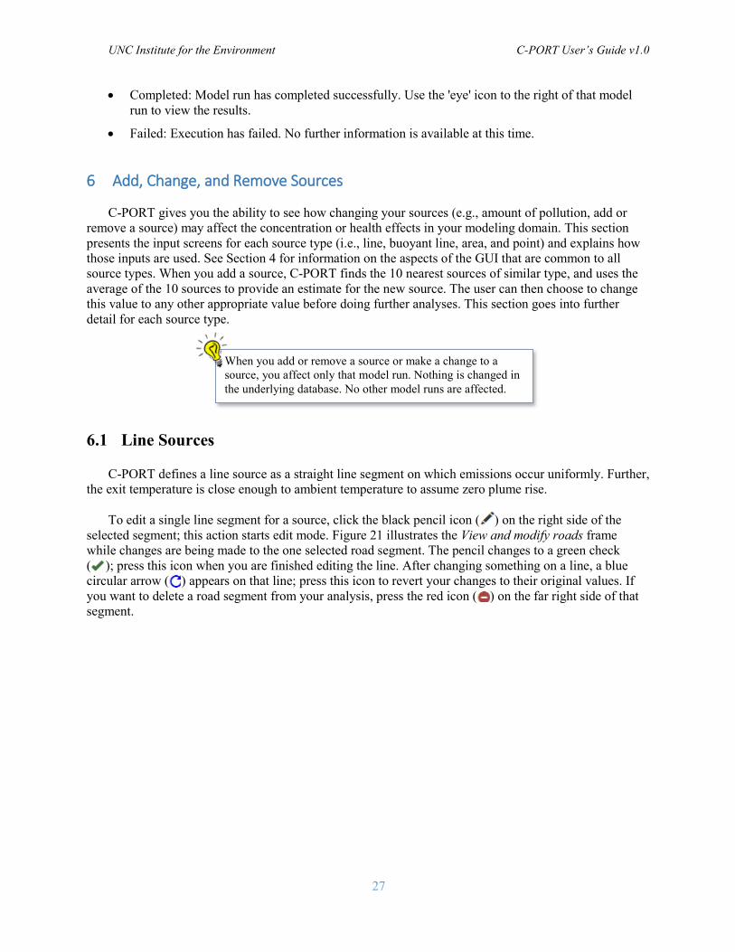
When you add or remove a source or make a change to a source, you affect only that model run. Nothing is changed in the underlying database. No other model runs are affected.
UNC Institute for the Environment C-PORT User’s Guide v1.0
28
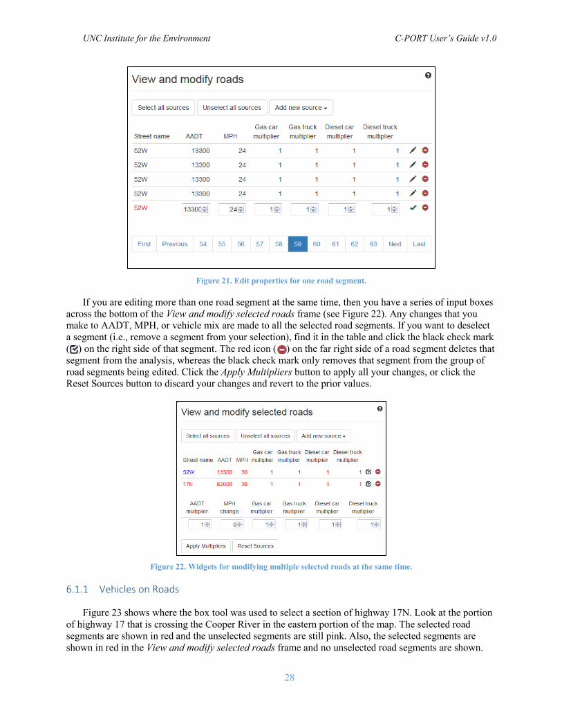
Figure 21. Edit properties for one road segment.
If you are editing more than one road segment at the same time, then you have a series of input boxes across the bottom of the View and modify selected roads frame (see Figure 22). Any changes that you make to AADT, MPH, or vehicle mix are made to all the selected road segments. If you want to deselect a segment (i.e., remove a segment from your selection), find it in the table and click the black check mark ( ) on the right side of that segment. The red icon ( ) on the far right side of a road segment deletes that segment from the analysis, whereas the black check mark only removes that segment from the group of road segments being edited. Click the Apply Multipliers button to apply all your changes, or click the Reset Sources button to discard your changes and revert to the prior values.
Figure 22. Widgets for modifying multiple selected roads at the same time.
6.1.1 Vehicles on Roads
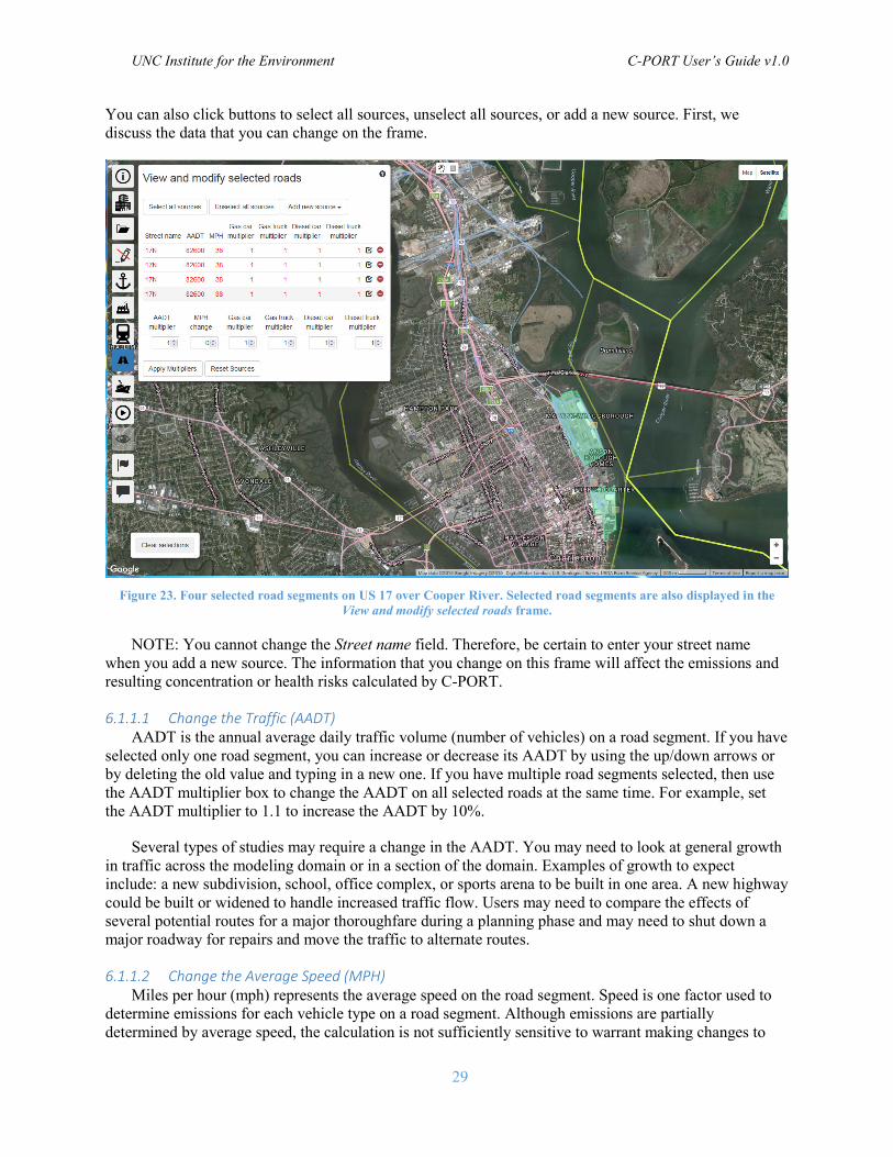
Figure 23 shows where the box tool was used to select a section of highway 17N. Look at the portion of highway 17 that is crossing the Cooper River in the eastern portion of the map. The selected road segments are shown in red and the unselected segments are still pink. Also, the selected segments are shown in red in the View and modify selected roads frame and no unselected road segments are shown.
UNC Institute for the Environment C-PORT User’s Guide v1.0
29
You can also click buttons to select all sources, unselect all sources, or add a new source. First, we discuss the data that you can change on the frame.
Figure 23. Four selected road segments on US 17 over Cooper River. Selected road segments are also displayed in the
View and modify selected roads frame.
NOTE: You cannot change the Street name field. Therefore, be certain to enter your street name when you add a new source. The information that you change on this frame will affect the emissions and resulting concentration or health risks calculated by C-PORT.
6.1.1.1 Change the Traffic (AADT) AADT is the annual average daily traffic volume (number of vehicles) on a road segment. If you have
selected only one road segment, you can increase or decrease its AADT by using the up/down arrows or by deleting the old value and typing in a new one. If you have multiple road segments selected, then use the AADT multiplier box to change the AADT on all selected roads at the same time. For example, set the AADT multiplier to 1.1 to increase the AADT by 10%.
Several types of studies may require a change in the AADT. You may need to look at general growth in traffic across the modeling domain or in a section of the domain. Examples of growth to expect include: a new subdivision, school, office complex, or sports arena to be built in one area. A new highway could be built or widened to handle increased traffic flow. Users may need to compare the effects of several potential routes for a major thoroughfare during a planning phase and may need to shut down a major roadway for repairs and move the traffic to alternate routes.
6.1.1.2 Change the Average Speed (MPH) Miles per hour (mph) represents the average speed on the road segment. Speed is one factor used to
determine emissions for each vehicle type on a road segment. Although emissions are partially determined by average speed, the calculation is not sufficiently sensitive to warrant making changes to
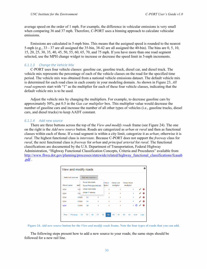
UNC Institute for the Environment C-PORT User’s Guide v1.0
30
average speed on the order of 1 mph. For example, the difference in vehicular emissions is very small when comparing 36 and 37 mph. Therefore, C-PORT uses a binning approach to calculate vehicular emissions.
Emissions are calculated in 5-mph bins. This means that the assigned speed is rounded to the nearest 5-mph (e.g., 33 - 37 are all assigned the 35-bin, 38-42 are all assigned the 40-bin). The bins are 0, 5, 10, 15, 20, 25, 30, 35, 40, 45, 50, 55, 60, 65, 70, and 75 mph. If you have more than one road segment selected, use the MPH change widget to increase or decrease the speed limit in 5-mph increments.
6.1.1.3 Change the Vehicle Mix C-PORT uses four vehicle classes: gasoline car, gasoline truck, diesel car, and diesel truck. The
vehicle mix represents the percentage of each of the vehicle classes on the road for the specified time period. The vehicle mix was obtained from a national vehicle emissions dataset. The default vehicle mix is determined for each road class in each county in your modeling domain. As shown in Figure 23, All road segments start with “1” as the multiplier for each of these four vehicle classes, indicating that the default vehicle mix is to be used.
Adjust the vehicle mix by changing the multipliers. For example, to decrease gasoline cars by approximately 50%, put 0.5 in the Gas car multiplier box. This multiplier value would decrease the number of gasoline cars and increase the number of all other types of vehicles (i.e., gasoline trucks, diesel cars, and diesel trucks) to keep AADT constant.
6.1.1.4 Add new source There are three buttons across the top of the View and modify roads frame (see Figure 24). The one
on the right is the Add new source button. Roads are categorized as urban or rural and then as functional classes within each of those. If a road segment is within a city limit, categorize it as urban; otherwise it is rural. The highest functional class is interstate. Because C-PORT does not support the freeway class for rural, the next functional class is freeway for urban and principal arterial for rural. The functional classifications are documented by the U.S. Department of Transportation, Federal Highway Administration, “Highway Functional Classification Concepts, Criteria and Procedures” available from http://www.fhwa.dot.gov/planning/processes/statewide/related/highway_functional_classifications/fcauab.pdf .
Figure 24. Add new source button for the View and modify roads frame. Note the four types of roads that you can add.
The following steps present how to add a new source to your roads; the same steps should be followed for a new rail line.
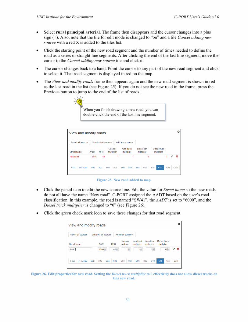
UNC Institute for the Environment C-PORT User’s Guide v1.0
31
• Select rural principal arterial. The frame then disappears and the cursor changes into a plus sign (+). Also, note that the tile for edit mode is changed to “on” and a tile Cancel adding new source with a red X is added to the tiles list.
• Click the starting point of the new road segment and the number of times needed to define the road as a series of straight line segments. After clicking the end of the last line segment, move the cursor to the Cancel adding new source tile and click it.
• The cursor changes back to a hand. Point the cursor to any part of the new road segment and click to select it. That road segment is displayed in red on the map.
• The View and modify roads frame then appears again and the new road segment is shown in red as the last road in the list (see Figure 25). If you do not see the new road in the frame, press the Previous button to jump to the end of the list of roads.
Figure 25. New road added to map.
• Click the pencil icon to edit the new source line. Edit the value for Street name so the new roads do not all have the name “New road”. C-PORT assigned the AADT based on the user’s road classification. In this example, the road is named “SW41”, the AADT is set to “6000”, and the Diesel truck multiplier is changed to “0” (see Figure 26).
• Click the green check mark icon to save these changes for that road segment.
Figure 26. Edit properties for new road. Setting the Diesel truck multiplier to 0 effectively does not allow diesel trucks on
this new road.
When you finish drawing a new road, you can double-click the end of the last line segment.
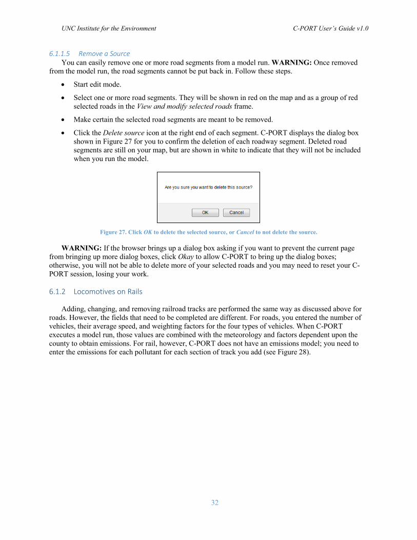
UNC Institute for the Environment C-PORT User’s Guide v1.0
32
6.1.1.5 Remove a Source You can easily remove one or more road segments from a model run. WARNING: Once removed
from the model run, the road segments cannot be put back in. Follow these steps.
• Start edit mode.
• Select one or more road segments. They will be shown in red on the map and as a group of red selected roads in the View and modify selected roads frame.
• Make certain the selected road segments are meant to be removed.
• Click the Delete source icon at the right end of each segment. C-PORT displays the dialog box shown in Figure 27 for you to confirm the deletion of each roadway segment. Deleted road segments are still on your map, but are shown in white to indicate that they will not be included when you run the model.
Figure 27. Click OK to delete the selected source, or Cancel to not delete the source.
WARNING: If the browser brings up a dialog box asking if you want to prevent the current page from bringing up more dialog boxes, click Okay to allow C-PORT to bring up the dialog boxes; otherwise, you will not be able to delete more of your selected roads and you may need to reset your C-PORT session, losing your work.
6.1.2 Locomotives on Rails
Adding, changing, and removing railroad tracks are performed the same way as discussed above for roads. However, the fields that need to be completed are different. For roads, you entered the number of vehicles, their average speed, and weighting factors for the four types of vehicles. When C-PORT executes a model run, those values are combined with the meteorology and factors dependent upon the county to obtain emissions. For rail, however, C-PORT does not have an emissions model; you need to enter the emissions for each pollutant for each section of track you add (see Figure 28).
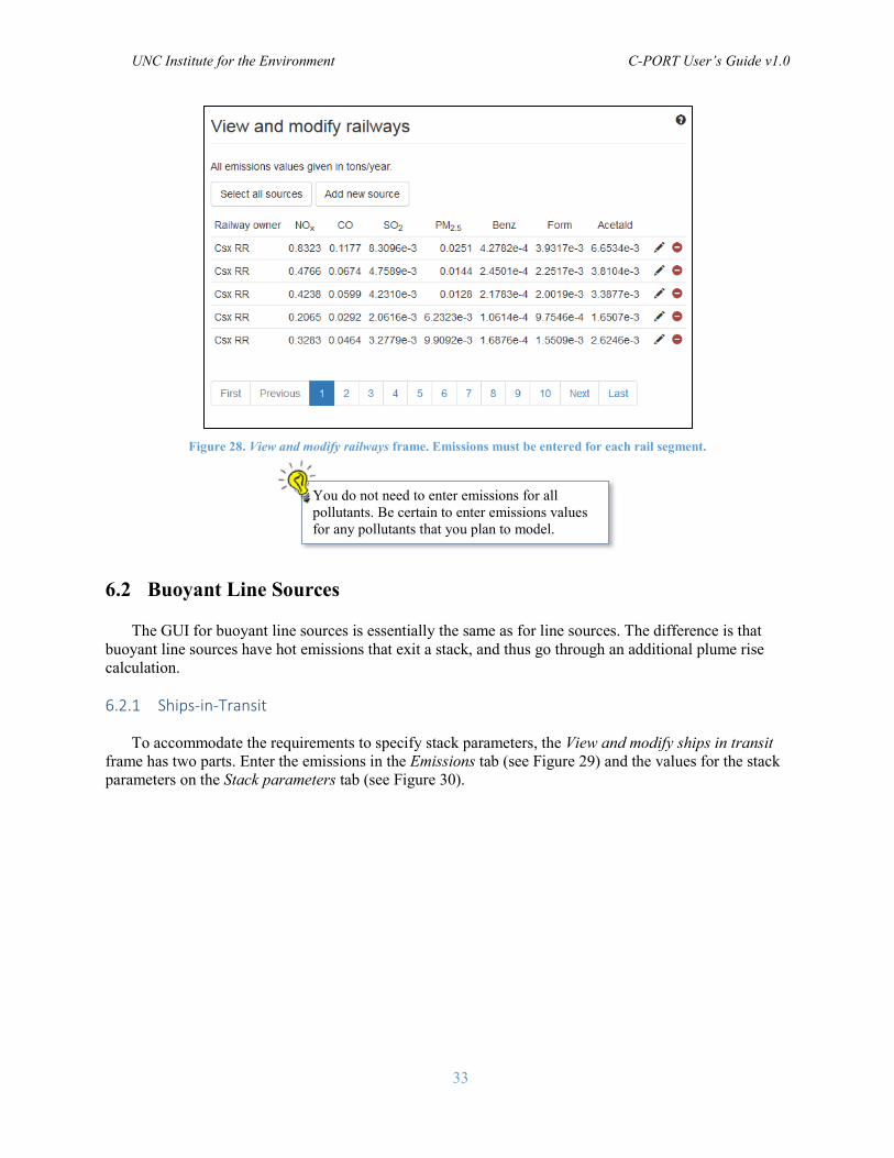
UNC Institute for the Environment C-PORT User’s Guide v1.0
33
Figure 28. View and modify railways frame. Emissions must be entered for each rail segment.
6.2 Buoyant Line Sources
The GUI for buoyant line sources is essentially the same as for line sources. The difference is that buoyant line sources have hot emissions that exit a stack, and thus go through an additional plume rise calculation.
6.2.1 Ships-in-Transit
To accommodate the requirements to specify stack parameters, the View and modify ships in transit frame has two parts. Enter the emissions in the Emissions tab (see Figure 29) and the values for the stack parameters on the Stack parameters tab (see Figure 30).
You do not need to enter emissions for all pollutants. Be certain to enter emissions values for any pollutants that you plan to model.
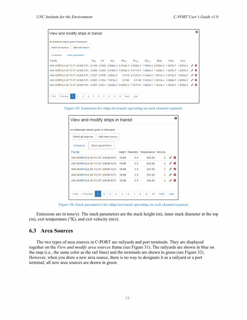
UNC Institute for the Environment C-PORT User’s Guide v1.0
34
Figure 29. Emissions for ships-in-transit operating on each channel segment.
Figure 30. Stack parameters for ships-in-transit operating on each channel segment.
Emissions are in tons/yr. The stack parameters are the stack height (m), inner stack diameter at the top (m), exit temperature (°K), and exit velocity (m/s).
6.3 Area Sources
The two types of area sources in C-PORT are railyards and port terminals. They are displayed together on the View and modify area sources frame (see Figure 31). The railyards are shown in blue on the map (i.e., the same color as the rail lines) and the terminals are shown in green (see Figure 32). However, when you draw a new area source, there is no way to designate it as a railyard or a port terminal; all new area sources are drawn in green.
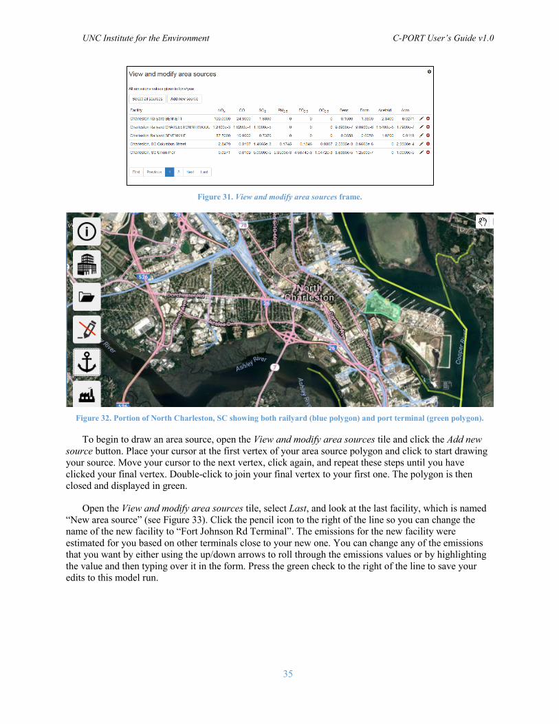
UNC Institute for the Environment C-PORT User’s Guide v1.0
35
Figure 31. View and modify area sources frame.
Figure 32. Portion of North Charleston, SC showing both railyard (blue polygon) and port terminal (green polygon).
To begin to draw an area source, open the View and modify area sources tile and click the Add new source button. Place your cursor at the first vertex of your area source polygon and click to start drawing your source. Move your cursor to the next vertex, click again, and repeat these steps until you have clicked your final vertex. Double-click to join your final vertex to your first one. The polygon is then closed and displayed in green.
Open the View and modify area sources tile, select Last, and look at the last facility, which is named “New area source” (see Figure 33). Click the pencil icon to the right of the line so you can change the name of the new facility to “Fort Johnson Rd Terminal”. The emissions for the new facility were estimated for you based on other terminals close to your new one. You can change any of the emissions that you want by either using the up/down arrows to roll through the emissions values or by highlighting the value and then typing over it in the form. Press the green check to the right of the line to save your edits to this model run.
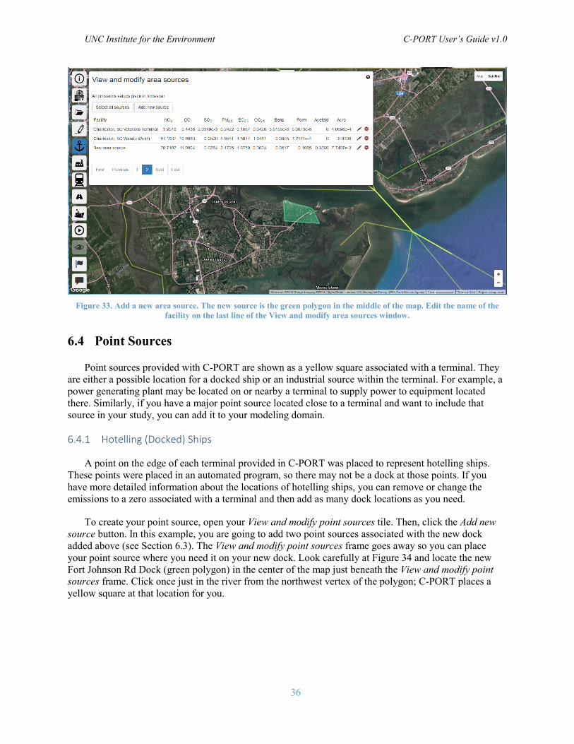
UNC Institute for the Environment C-PORT User’s Guide v1.0
36
Figure 33. Add a new area source. The new source is the green polygon in the middle of the map. Edit the name of the
facility on the last line of the View and modify area sources window.
6.4 Point Sources
Point sources provided with C-PORT are shown as a yellow square associated with a terminal. They are either a possible location for a docked ship or an industrial source within the terminal. For example, a power generating plant may be located on or nearby a terminal to supply power to equipment located there. Similarly, if you have a major point source located close to a terminal and want to include that source in your study, you can add it to your modeling domain.
6.4.1 Hotelling (Docked) Ships
A point on the edge of each terminal provided in C-PORT was placed to represent hotelling ships. These points were placed in an automated program, so there may not be a dock at those points. If you have more detailed information about the locations of hotelling ships, you can remove or change the emissions to a zero associated with a terminal and then add as many dock locations as you need.
To create your point source, open your View and modify point sources tile. Then, click the Add new source button. In this example, you are going to add two point sources associated with the new dock added above (see Section 6.3). The View and modify point sources frame goes away so you can place your point source where you need it on your new dock. Look carefully at Figure 34 and locate the new Fort Johnson Rd Dock (green polygon) in the center of the map just beneath the View and modify point sources frame. Click once just in the river from the northwest vertex of the polygon; C-PORT places a yellow square at that location for you.
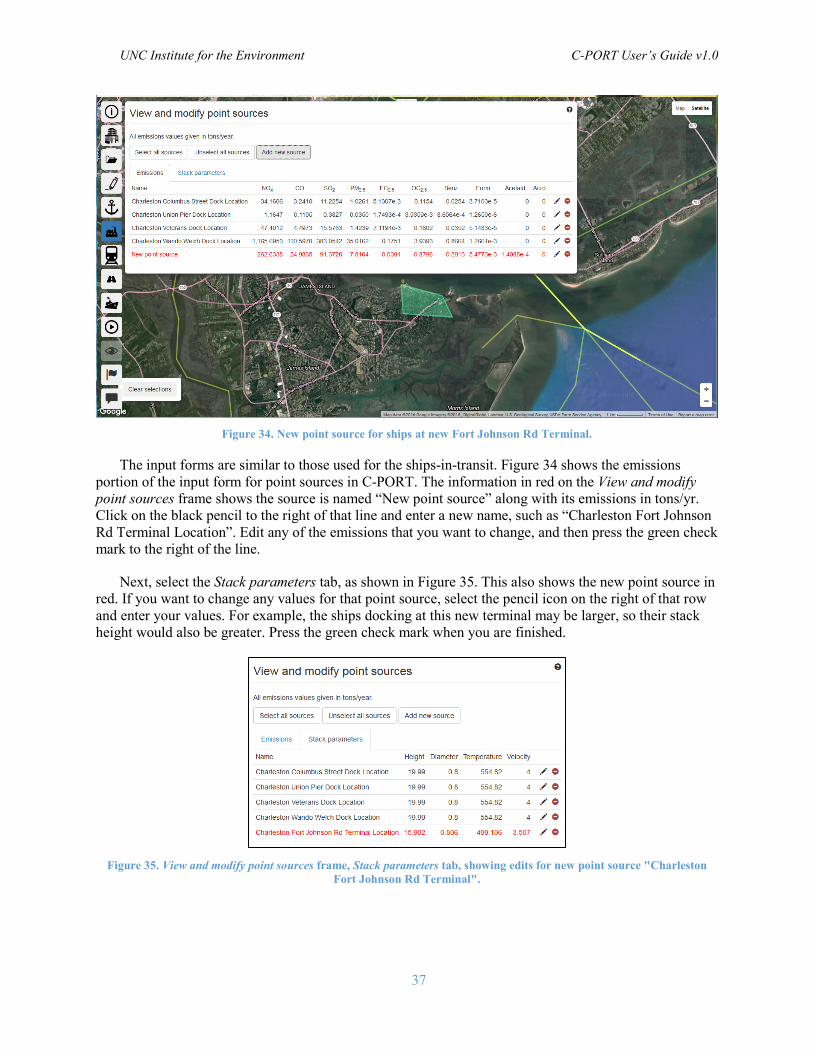
UNC Institute for the Environment C-PORT User’s Guide v1.0
37
Figure 34. New point source for ships at new Fort Johnson Rd Terminal.
The input forms are similar to those used for the ships-in-transit. Figure 34 shows the emissions portion of the input form for point sources in C-PORT. The information in red on the View and modify point sources frame shows the source is named “New point source” along with its emissions in tons/yr. Click on the black pencil to the right of that line and enter a new name, such as “Charleston Fort Johnson Rd Terminal Location”. Edit any of the emissions that you want to change, and then press the green check mark to the right of the line.
Next, select the Stack parameters tab, as shown in Figure 35. This also shows the new point source in red. If you want to change any values for that point source, select the pencil icon on the right of that row and enter your values. For example, the ships docking at this new terminal may be larger, so their stack height would also be greater. Press the green check mark when you are finished.
Figure 35. View and modify point sources frame, Stack parameters tab, showing edits for new point source "Charleston
Fort Johnson Rd Terminal".
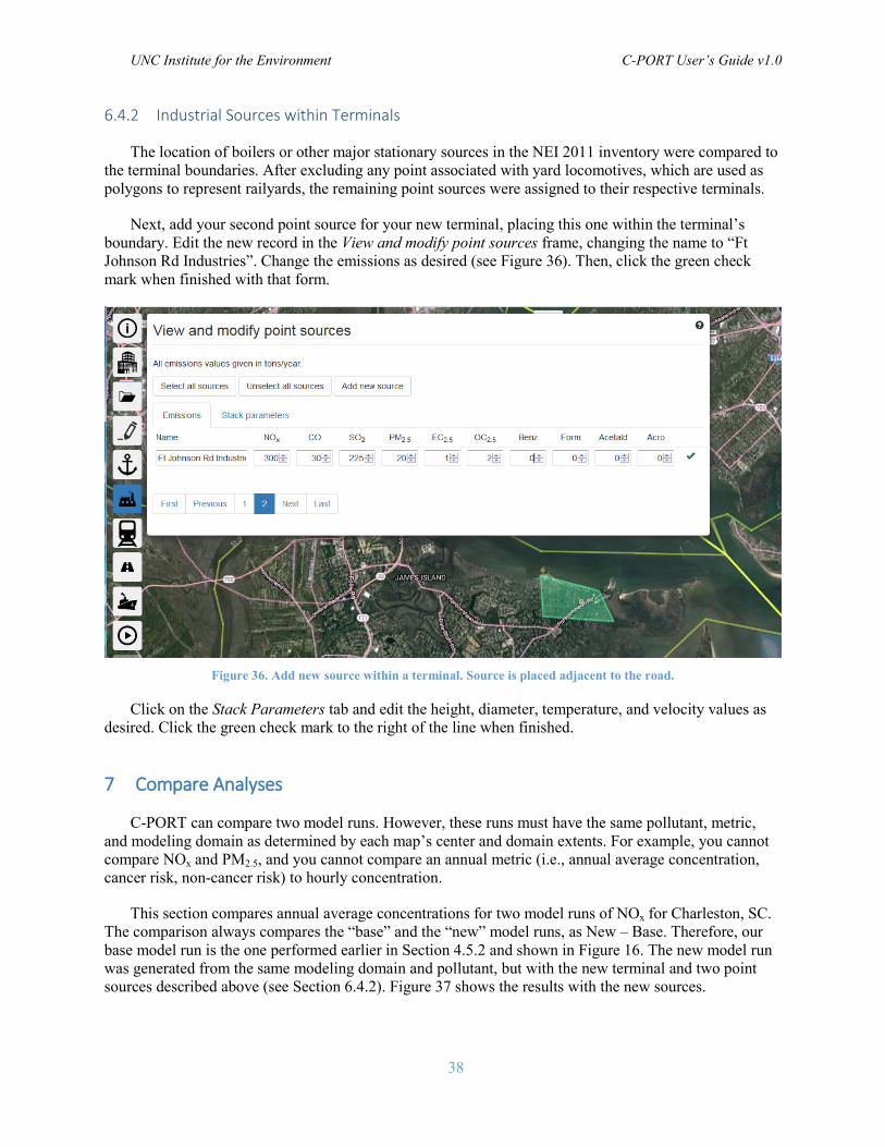
UNC Institute for the Environment C-PORT User’s Guide v1.0
38
6.4.2 Industrial Sources within Terminals
The location of boilers or other major stationary sources in the NEI 2011 inventory were compared to the terminal boundaries. After excluding any point associated with yard locomotives, which are used as polygons to represent railyards, the remaining point sources were assigned to their respective terminals.
Next, add your second point source for your new terminal, placing this one within the terminal’s boundary. Edit the new record in the View and modify point sources frame, changing the name to “Ft Johnson Rd Industries”. Change the emissions as desired (see Figure 36). Then, click the green check mark when finished with that form.
Figure 36. Add new source within a terminal. Source is placed adjacent to the road.
Click on the Stack Parameters tab and edit the height, diameter, temperature, and velocity values as desired. Click the green check mark to the right of the line when finished.
7 Compare Analyses
C-PORT can compare two model runs. However, these runs must have the same pollutant, metric, and modeling domain as determined by each map’s center and domain extents. For example, you cannot compare NOx and PM2.5, and you cannot compare an annual metric (i.e., annual average concentration, cancer risk, non-cancer risk) to hourly concentration.
This section compares annual average concentrations for two model runs of NOx for Charleston, SC. The comparison always compares the “base” and the “new” model runs, as New – Base. Therefore, our base model run is the one performed earlier in Section 4.5.2 and shown in Figure 16. The new model run was generated from the same modeling domain and pollutant, but with the new terminal and two point sources described above (see Section 6.4.2). Figure 37 shows the results with the new sources.
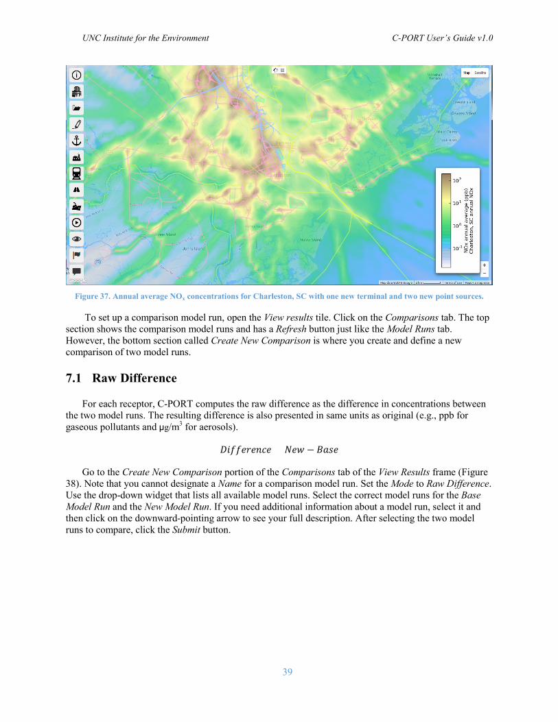
UNC Institute for the Environment C-PORT User’s Guide v1.0
39
Figure 37. Annual average NOx concentrations for Charleston, SC with one new terminal and two new point sources.
To set up a comparison model run, open the View results tile. Click on the Comparisons tab. The top section shows the comparison model runs and has a Refresh button just like the Model Runs tab. However, the bottom section called Create New Comparison is where you create and define a new comparison of two model runs.
7.1 Raw Difference
For each receptor, C-PORT computes the raw difference as the difference in concentrations between the two model runs. The resulting difference is also presented in same units as original (e.g., ppb for gaseous pollutants and μg/m3 for aerosols).
𝐷𝐷𝐷𝐷𝐷𝐷𝐷𝐷𝐷𝐷𝐷𝐷𝐷𝐷𝐷𝐷𝐷𝐷𝐷𝐷 = 𝑁𝑁𝐷𝐷𝑁𝑁 − 𝐵𝐵𝐵𝐵𝐵𝐵𝐷𝐷
Go to the Create New Comparison portion of the Comparisons tab of the View Results frame (Figure 38). Note that you cannot designate a Name for a comparison model run. Set the Mode to Raw Difference. Use the drop-down widget that lists all available model runs. Select the correct model runs for the Base Model Run and the New Model Run. If you need additional information about a model run, select it and then click on the downward-pointing arrow to see your full description. After selecting the two model runs to compare, click the Submit button.
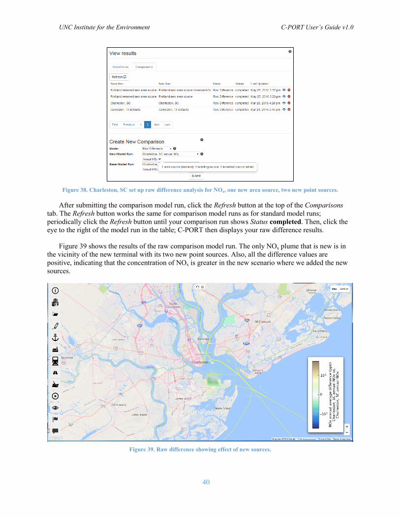
UNC Institute for the Environment C-PORT User’s Guide v1.0
40
Figure 38. Charleston, SC set up raw difference analysis for NOx, one new area source, two new point sources.
After submitting the comparison model run, click the Refresh button at the top of the Comparisons tab. The Refresh button works the same for comparison model runs as for standard model runs; periodically click the Refresh button until your comparison run shows Status completed. Then, click the eye to the right of the model run in the table; C-PORT then displays your raw difference results.
Figure 39 shows the results of the raw comparison model run. The only NOx plume that is new is in the vicinity of the new terminal with its two new point sources. Also, all the difference values are positive, indicating that the concentration of NOx is greater in the new scenario where we added the new sources.
Figure 39. Raw difference showing effect of new sources.
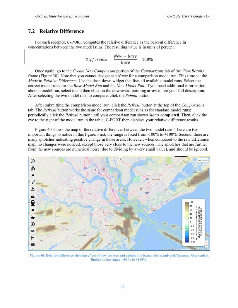
UNC Institute for the Environment C-PORT User’s Guide v1.0
41
7.2 Relative Difference
For each receptor, C-PORT computes the relative difference as the percent difference in concentrations between the two model runs. The resulting value is in units of percent.
𝐷𝐷𝐷𝐷𝐷𝐷𝐷𝐷𝐷𝐷𝐷𝐷𝐷𝐷𝐷𝐷𝐷𝐷𝐷𝐷 = 𝑁𝑁𝐷𝐷𝑁𝑁 − 𝐵𝐵𝐵𝐵𝐵𝐵𝐷𝐷
𝐵𝐵𝐵𝐵𝐵𝐵𝐷𝐷× 100%
Once again, go to the Create New Comparison portion of the Comparisons tab of the View Results frame (Figure 38). Note that you cannot designate a Name for a comparison model run. This time set the Mode to Relative Difference. Use the drop-down widget that lists all available model runs. Select the correct model runs for the Base Model Run and the New Model Run. If you need additional information about a model run, select it and then click on the downward-pointing arrow to see your full description. After selecting the two model runs to compare, click the Submit button.
After submitting the comparison model run, click the Refresh button at the top of the Comparisons tab. The Refresh button works the same for comparison model runs as for standard model runs; periodically click the Refresh button until your comparison run shows Status completed. Then, click the eye to the right of the model run in the table; C-PORT then displays your relative difference results.
Figure 40 shows the map of the relative differences between the two model runs. There are two important things to notice in this figure. First, the range is fixed from -100% to +100%. Second, there are many splotches indicating positive change in those areas. However, when compared to the raw difference map, no changes were noticed, except those very close to the new sources. The splotches that are further from the new sources are numerical noise (due to dividing by a very small value), and should be ignored.
Figure 40. Relative difference showing effect of new sources and calculation issues with relative differences. Note scale is
limited to the range -100% to +100%.

UNC Institute for the Environment C-PORT User’s Guide v1.0
42
8 User Feedback
Click on the tile at the bottom of the list of tiles on the left side of the C-PORT screen to provide comments about this product and your user experience. This icon directs you to a very short survey and a free-form text box to provide comments. We encourage all C-PORT users to provide feedback for future enhancements.