User Manual

UK DCP 2.2

Measurement of Road Pavement Strength by

Dynamic Cone Penetrometer

by Simon Done and Piouslin Samuel

Unpublished Project Report

PR INT/278/04Project Record No R8157

ii

PROJECT REPORT PR/INT/278/04

Measurement of Road Pavement Strength by Dynamic Cone Penetrometer

Simon Done and Piouslin Samuel

Sector: Transport

Theme: T2: Reduce overall transport cost by cost effective road rehabilitationand maintenance

Project Title: Improved Measurement of Road Pavement Strength by DynamicCone Penetrometer

Project Reference: R8157

Approvals

Project Manager

Quality Reviewed

Copyright TRL Limited May 2004This document has been prepared as part of a project funded by the UK Departmentfor International Development (DFID) for the benefit of developing countries. The viewsexpressed are not necessarily those of DFID.

The Transport Research Laboratory and TRL are trading names of TRL Limited, a member of theTransport Research Foundation Group of Companies.

TRL Limited. Registered in England, Number 3142272. Registered Office: Old Wokingham Road,Crowthorne, Berkshire, RG45 6AU, United Kingdom.

iii

ACKNOWLEDGEMENTS

The development of UK DCP software has been based upon the responses received toa questionnaire distributed to the members of the International Focus Group (IFG). Weare extremely grateful to those who took the time to complete the questionnaire andreturn it to us. We are also grateful to Dr Stephen Morris and James Painter of TessellaSupport Services plc who wrote the software and Yogita Maini of DFID and Phil Page-Green of CSIR, South Africa, who reviewed the project and provided useful feedback.The TRL team responsible for analysing the questionnaires, designing the software,writing the user manual and making UK DCP available were Piouslin Samuel, ColinJones, Simon Done, Dr John Rolt, Dave Weston and Trevor Bradbury.

May 2004

iv

Contents

1 Introduction .............................................................................................................1

2 Installation ...............................................................................................................5

2.1 Obtaining UK DCP.........................................................................................5

2.2 Installing UK DCP..........................................................................................52.2.1 Installation from CD ...................................................................................52.2.2 Installation from Transport Links website ..................................................5

2.3 Uninstalling UK DCP......................................................................................6

3 Start up....................................................................................................................7

3.1 Run UK DCP..................................................................................................73.1.1 Start a new project.....................................................................................83.1.2 Open an existing project............................................................................93.1.3 Closing a project and exiting UK DCP.......................................................9

3.2 Test Manager .................................................................................................9

4 Data input..............................................................................................................11

4.1 Introduction...................................................................................................11

4.2 Site details ....................................................................................................12

4.3 Upper layers.................................................................................................134.3.1 Layers removed .......................................................................................134.3.2 Upper layer details ...................................................................................14

4.4 Penetration data...........................................................................................164.4.1 Site details summary ...............................................................................164.4.2 Penetration data.......................................................................................16

4.5 Set-Up ..........................................................................................................204.5.1 Analysis ....................................................................................................214.5.2 Sectioning.................................................................................................214.5.3 CBR Calculation.......................................................................................224.5.4 Other Options...........................................................................................23

5 Layer analysis .......................................................................................................24

5.1 Introduction...................................................................................................24

5.2 Analysing Test layers...................................................................................24

5.3 Automatic layer analysis ..............................................................................25

5.4 Manual layer analysis ..................................................................................29

5.5 Analysis of drilled and very strong layers ....................................................365.5.1 Drilled layers ............................................................................................375.5.2 Very strong layers ....................................................................................39

6 Structural Number calculation ..............................................................................41

6.1 Introduction...................................................................................................416.1.1 Upper layers.............................................................................................416.1.2 Base and Sub-base Test layers ..............................................................416.1.3 Subgrade Test layers...............................................................................42

6.2 Calculating the Structural Number...............................................................426.2.1 Upper layers.............................................................................................43

v

6.2.2 Test layers................................................................................................446.2.3 SN Calculation Buttons ............................................................................456.2.4 Pavement Strength ..................................................................................48

7 Query ....................................................................................................................50

7.1 Introduction...................................................................................................50

7.2 Making a Query............................................................................................507.2.1 Query Parameter .....................................................................................517.2.2 Tests Included..........................................................................................517.2.3 Query Type...............................................................................................517.2.4 Display Options ........................................................................................51

7.3 Displaying the Query results ........................................................................517.3.1 Structural Number....................................................................................527.3.2 Layer or Pavement Thickness .................................................................537.3.3 CBR..........................................................................................................54

8 Sectioning .............................................................................................................56

8.1 Introduction...................................................................................................56

8.2 Sections box.................................................................................................578.2.1 Parameters ..............................................................................................578.2.2 Tests Included..........................................................................................588.2.3 Sections Buttons ......................................................................................58

8.3 Sectioning a project......................................................................................598.3.1 Determine Sections by parameter...........................................................598.3.2 Determine Design Sections for the project..............................................62

9 Reporting...............................................................................................................66

9.1 Introduction...................................................................................................66

9.2 Test Reports ................................................................................................679.2.1 Penetration Data ......................................................................................679.2.2 Layer Strength Analysis ...........................................................................69

9.3 Project Reports ............................................................................................719.3.1 Section Summary.....................................................................................719.3.2 Design Section Properties .......................................................................729.3.3 Project Summary .....................................................................................73

10 References ...........................................................................................................74

vi

List of Figures

Figure 1.1 DCP instrument ................................................................................................2Figure 3.1 Flash screen.....................................................................................................7Figure 3.2 Welcome box....................................................................................................8Figure 3.3 Test Manager (without test data)......................................................................8Figure 3.4 Test Manager (with test data and completed analysis)...................................9Figure 4.1 Test Details box ..............................................................................................11Figure 4.2 Illustration of Upper layers, Test layers and Removed layers.......................14Figure 4.3 Penetration Data box (with test data).............................................................16Figure 4.4 Penetration Data box (with a drilled layer and an extension rod)..................20Figure 4.5 Set-Up Options box ........................................................................................21Figure 4.6 Test Manager (showing that test data has been input) .................................23Figure 5.1 How Automatic analysis works ......................................................................26Figure 5.2 Layer Boundaries box using Automatic layer analysis ..................................26Figure 5.3 Test Manager (showing that test data has been analysed)...........................28Figure 5.4 Layer Boundaries box using Manual layer analysis ......................................30Figure 5.5 Test Manager (showing that test data has been analysed)...........................32Figure 5.6 Double intersections .......................................................................................34Figure 5.7 Negative gradient............................................................................................34Figure 5.8 Line does not intersect the line of test points.................................................35Figure 5.9 Line drawn parallel to its intended position ....................................................35Figure 5.10 Line moved laterally to its intended position ................................................36Figure 5.11 Lines overlap but do not intersect................................................................36Figure 5.12 Automatic analysis of a drilled layer.............................................................37Figure 5.13 Manual analysis of a drilled layer and the use of gaps................................38Figure 5.14 Automatic analysis of a very strong layer ....................................................39Figure 5.15 Manual analysis of a very strong layer and the use of gaps .......................40Figure 6.1 SN Calculation box (before calculating SNs).................................................43Figure 6.2 Layer Boundaries box.....................................................................................45Figure 6.3 Adjusted Penetration Data box.......................................................................46Figure 6.4 CBR Chart box................................................................................................46Figure 6.5 SN Calculation box (after calculations are complete)....................................48Figure 6.6 Test Manager (showing that SNs have been calculated)..............................49Figure 7.1 Query box .......................................................................................................50Figure 7.2 Structural Number histogram .........................................................................52Figure 7.3 Layer Thickness histogram ............................................................................53Figure 7.4 CBR histogram (Minimum).............................................................................54Figure 7.5 CBR histogram (Less Than) ..........................................................................55Figure 8.1 Sections box (before sectioning)....................................................................57Figure 8.2 Uniform Sections box .....................................................................................59Figure 8.3 Histogram of sectioning data..........................................................................61Figure 8.4 Uniform Sections box (with one section boundary added) ............................61Figure 8.5 Sections box (after Sectioning) ......................................................................62Figure 8.6 Section Summary box ....................................................................................62Figure 8.7 Design Section Properties box.......................................................................64Figure 8.8 Section Summary box (with one Design Section boundary added) ..............64Figure 8.9 Test Manager (showing that Design Sections have been defined)...............65Figure 9.1 Export box.......................................................................................................66Figure 9.2 Penetration Data Report.................................................................................67Figure 9.3 Layer Strength Analysis Report .....................................................................69Figure 9.4 Section Summary Report ...............................................................................71Figure 9.5 Design Section Properties Report..................................................................72Figure 9.6 Project Summary Report................................................................................73

vii

List of Tables

Table 4.1 Penetration rate – CBR relationships ..............................................................22Table 5.1 Example of penetration data and cumulative difference sum analysis ..........27Table 6.1 CBR – Strength Coefficient (a) relationships ..................................................42

List of Boxes

Box 1.1 Key points to know before starting to use UK DCP........................................ 4Box 4.1 Recording the removal of very thick Upper layers........................................ 15Box 4.2 Calculating adjusted penetration data........................................................... 17Box 5.1 Should penetration data be analysed automatically or manually? ............... 25Box 5.2 Corrected analysis of deep surface texture and disturbed soil..................... 29Box 5.3 Analysis of a drilled layer............................................................................... 38Box 5.4 Analysis of a very strong but penetrable layer.............................................. 40Box 6.1 The importance of checking the layer analysis against the CBR Chart....... 47

1

1 Introduction

When required to assess the strength of a pavement or to design improvementworks, the pavement engineer needs to know as much as possible about thethicknesses of the existing pavement layers and their condition. In some cases thequickest and easiest way to do this is to inspect the design to which the pavementwas originally built and perhaps also the as-built records made during construction.However, designs indicate only an intended construction and as-built records areoften only indicative of the construction work carried out. Furthermore, both designsand as-built records give no information as to what has happened to the pavementsince construction and the condition it is currently in. To give useful information, it istherefore necessary to investigate the current pavement condition using some formof destructive or non destructive testing.

The usual method of destructive testing is to dig test pits at suitable intervals alongthe road. These are very useful as pavement thicknesses can be measured andmaterial removed for testing in a laboratory. However, test pits are expensive to digand reinstate and are rarely dug at intervals of less than 2-3 kilometres.

The Dynamic Cone Penetrometer (DCP) (Figure 1.1), is an efficient way of testingpavement at more frequent intervals. Tests using the DCP generate data which canbe analysed to produce accurate information on in situ pavement layer thicknessesand strengths. Tests can be carried out very rapidly and test sites can be repairedextremely easily. A typical DCP test team of 3 people may be able to carry out 20tests in a day at a spacing of between 50 and 500 metres. The DCP can thereforegive information of sufficient quality and quantity to allow the pavement strength tobe estimated and improvement works designed. Results from DCP tests can also beused to locate test pits in the most suitable positions.

The DCP consists of a cone fixed to the bottom of a tall vertical rod. A weight isrepeatedly lifted and dropped onto a coupling at the mid-height of the rod to deliver astandard impact, or ‘blow’, to the cone and drive it into the pavement. A vertical scalealongside the rod is used to measure the depth of penetration of the cone. Thepenetration per blow, the ‘penetration rate’, is recorded as the cone is driven into thepavement and then used to calculate the strength of the material through which it ispassing. A change in penetration rate indicates a change in strength betweenmaterials, thus allowing layers to be identified and the thickness and strength of eachto be determined. These layers are then grouped together into the pavement layersof base, sub-base and subgrade, guided by test pit or as-built records if available.

The DCP cannot penetrate some strong surface and base materials such as hot mixasphalt or cement treated bases. These layers must be removed before the test canbegin and their strength assessed using different criteria.

The strengths of all layers can then be combined into a Structural Number for eachpavement layer and the entire pavement structure. Where tests are repeated alongthe pavement, a longitudinal picture of the pavement can be developed which allowschanges in construction and condition to be identified. This data can then be used todivide the road into homogeneous sections.

2

Figure 1.1 DCP instrument

This manual guides users of this UK DCP software. It has 9 chapters, eachdescribing one stage or function of its installation and operation.

No. Title Description

1 Introduction

2 Installation Obtain and install UK DCP.

3 Start up Run UK DCP and open a new or existing project. The term project refersto a set of related sites, at each of which a penetration test has beencarried out and which will be analysed together. In normal use, a projectwill be a single road or a length of apparently uniform construction.

4 Data input Input site details and penetration data for the tests within a project.

5 Layeranalysis

Analyse the penetration data from a test to identify, and determine thethicknesses of the distinct Test layers within the pavement. Layeridentification can be carried out manually or automatically.

6 StructuralNumbercalculation

Assign the Test layers to specific pavement layers and calculate theStructural Number of each pavement layer.

7 Query Produce histograms of strengths and pavement layer thicknesses alongthe project. The primary purpose of this function is to identify any errorsmade during data entry and analysis.

8 Sectioning Divide a project into uniform sections.

9 Reporting Produce reports of the data, analysis and results for printing or export.

3

UK DCP was written in Visual Basic language and uses a Microsoft Access databaseto store the data, although it is not necessary for Microsoft Access itself to beinstalled on the computer. It will run on Windows 98, NT, 2000 and XP operatingsystems and ideally requires a computer with a minimum specification of 400 MHz,64 MB of memory and 45 MB of free disk space , although it should still runsuccessfully, albeit slightly more slowly, on a computer of lower specification.

UK DCP is not intended to replace normal engineering judgement. The proceduresused are intended for users who already have a thorough understanding of DCPanalysis and are capable of deciding which method of analysis is most appropriatefor individual situations. The user must be aware of the limitations of this programand, most importantly, that incorrect data input will lead to incorrect output. The usershould be capable of assessing the accuracy of any results produced. No warrantycan be given on the validity of results and the ultimate responsibility for acceptanceand subsequent use of any results lies solely with the user. TRL Limited cannotaccept any liability for any error or omission.

Some of the limitations of the use of DCP and this package are:

UK DCP can analyse DCP data collected from existing flexible pavementsconstructed with unbound materials. Very little difficulty is experienced with thepenetration of granular pavement layers or lightly stabilised material. It is, however,often not possible to penetrate coarse granular materials, material stabilised with ahigh percentage of cement or thick layers of bituminous material. In such cases it isnecessary to drill a hole through the impenetrable layer and then continue gatheringDCP penetration data in the underlying material. Because penetration data can notbe recorded for the drilled layer, it is necessary to estimate and input the strengthcoefficient for the layer in order to assess its contribution to the Structural Number ofthe pavement.

Thin bituminous layers, such as a surface dressing, can be penetrated by the DCP,although the data is not used to calculate the strength of such layers, and as suchthe strength coefficient must be estimated.

UK DCP cannot analyse penetration data which includes two drilled layers below thesurface. If it proves necessary to drill twice, it is recommended that a test is repeatedor that the test result be analysed manually.

The DCP instrument with an extension rod of 400 mm can be used to a depth of only1200 mm. Although the instrument can be extended beyond this depth, withadditional extension rods or extension road longer than 400 mm, it is notrecommended that this is done as friction between the rod and the soil can giveunreliable data. However, UK DCP has been designed to accept data up to amaximum depth of 1500 mm.

The output from DCP results is controlled by the user as follows:• Selecting an appropriate CBR – DCP penetration relationship as explained in

4.5.3. CBR Calculation.• The user’s identification of the base, sub-base and subgrade layers as

explained in 5. Layer Analysis.• Selection of appropriate parameters for dividing the project into shorter

sections of uniform strength as explained in 8. Sectioning.

4

UK DCP is available free of charge to all who wish to use it.

Box 1.1 Key points to know before starting to use UK DCP

Context sensitive help is available at all stages. This manual can also be displayed andprinted through the Help menu at the top of the main window.

Data and results do not have to be saved manually. Whenever data is entered into a box andthe box is closed by clicking an OK button, its contents are automatically saved.

Only one set of penetration tests (a ‘project’) can be opened at any one time, but many ofthose tests can be examined simultaneously and compared.

When a number of windows and boxes are open, they can be selected for display using theWindow menu at the top of the main window.

In this manual all software images have been taken from a single project. Two images at thesame chainage represent the same data and later sectioning images are based uponpenetration data in earlier images.

5

2 Installation

2.1 Obtaining UK DCP

UK DCP can be obtained by contacting TRL:

TRL LimitedCrowthorne HouseNine Mile RideWokinghamBerkshireRG40 3GAUnited Kingdom

Tel: + 44 (0) 1344 770187Fax: +44 (0) 1344 770356Email: international_enquiries@trl.co.ukWeb: www.trl.co.uk

Alternatively, UK DCP is available on the Road Engineering for Development CD,distributed by TRL, or as a download from the Transport Links website. The addressof this website is www.transport-links.org/ukdcp

2.2 Installing UK DCP

Before installing UK DCP, it is recommended that any earlier versions of the softwareare uninstalled (2.3) and, if there are any data files from previous analysis to besaved, the UK DCP directory is moved from the Program Files directory to a differentlocation. The total size of the files which must be downloaded for installation is11.6MB.

2.2.1 Installation from CD

This procedure will install UK DCP, all necessary third party software and help filesonto the user’s computer. For computers with Windows 2000 or NT, follow steps 1 to4 below. For computers with Windows 98 or XP, follow steps 1 to 6.

1. Open the UK DCP folder on the CD.2. Double-click or run the file named ‘setup.exe’.3. When prompted, select the directory in which UK DCP will be installed. By

default, ‘C:\Program Files\UKDCP’ is selected.4. When the setup program is complete, a new item, ‘UK DCP’, will be added to

the Start/Programs menu.

5. In the UK DCP folder, double-click or run the file named ‘MDAC_TYP.exe’.6. When this setup program is complete, reboot the computer.

2.2.2 Installation from Transport Links website

The procedure to download all relevant files and install UK DCP, all necessary thirdparty software and help files onto the user’s computer from the Transport Linkswebsite is very simple. Click on UK DCP Installer. Downloading and installation willtake place automatically. For computers with Windows 98 or XP, it is then necessaryto click on ‘MDAC_TYP.exe’, wait for the setup programme to finish and reboot thecomputer.

6

2.3 Uninstalling UK DCP

This procedure will uninstall UK DCP from the user’s computer. It may vary slightlydepending upon which Windows operating system is installed on the computer.

1. Select Settings from the Start menu.2. Select Control Panel.3. Double-click Add or Remove Programs.4. Highlight the version of UK DCP to be removed.5. Click Change/Remove.6. This will not completely delete all files. When uninstallation is complete, open

Windows Explorer and then navigate to the folder in which UK DCP wasinstalled. Delete the folder and its contents. If the warning “Renaming, movingor deleting ‘ukdcp’ could make some programs not work. Are you sure thatyou want to do this?” is generated, click Yes and continue with the deletion.

7

3 Start up

This chapter describes how to run UK DCP and introduces the Test Manager.

3.1 Run UK DCP

UK DCP can be run by either clicking a desktop icon or through the Programs menuon the Start button. After a brief Flash screen (Figure 3.1), the Main window will openwith a Welcome box (Figure 3.2). The Welcome box allows a new or existing projectto be opened and also contains a list of the most recently used projects. The sameoptions are available in the File menu at the top of the main window.

Figure 3.1 Flash screen

8

Figure 3.2 Welcome box

3.1.1 Start a new project

Click New Project in the Welcome box or in the File menu at the top of the mainwindow. This will generate a Save New Project As box. Give a name to the newproject, select a folder in which to save it and click Save. The project will beautomatically given a .ukdcp file extension and saved in the selected folder. Anempty Test Manager box (Figure 3.3) will open for the new project with its name atthe top. Since only one project can be open within UK DCP at any time, if a project iscurrently open and a new project is named and saved, a message will be generatedseeking confirmation that the current project should be closed. If Yes is clicked, thecurrent project will be closed and the new project opened.

Figure 3.3 Test Manager (without test data)

9

3.1.2 Open an existing project

Click Open Existing Project in the Welcome box or Open Project in the File menu atthe top of the main window. This will generate an Open Existing Project box in whichthe file of the required project can be found and selected. Highlight the file and clickOpen. A Test Manager filled with the existing data and analysis will open (Figure 3.4shows a Test Manager of a project which has been fully analysed). Alternatively,double-click on the required file in the Recent Files list in the Welcome box or in theFile menu and the Test Manager will open. Since only one project can be open withinUK DCP at any time, if a project is currently open and an existing project is selected,a message will be generated seeking confirmation that the current project should beclosed. If Yes is clicked, the current project will be closed and the selected projectopened.

Figure 3.4 Test Manager (with test data and completed analysis)

3.1.3 Closing a project and exiting UK DCP.

Only one project can be run by UK DCP at any time. To close a project, click Closein the Test Manager. A box will be generated seeking confirmation. Click Yes toclose the project. To exit UK DCP, click Exit in the File menu at the top of the mainwindow. A box will be generated seeking confirmation. Click Yes to exit.

3.2 Test Manager

The Test Manager (empty: Figure 3.3, or complete: Figure 3.4) is used to store alldata from the project and manage data entry, layer analysis, strength calculations,queries and project sectioning. Each row of the table in the Test Manager representsone penetration test and shows the progress that has been made in analysing thedata from both the individual test and the entire project.

10

The table in the Test Manager has five columns.

Test number Tests are automatically numbered in chainage order from 1 upwards. If morethan one test is carried out at the same chainage, they are ordered accordingto their location (carriageway; shoulder; verge; lay-by / other – see 4.2 below).If more than one test is carried out at the same chainage in the carriageway,they are ordered according to their lane number and offset (see 4.2 below). Ifmore than one test is carried out at the same chainage off the carriageway,they are ordered according to their offset. There is no limit to the number oftests that can be entered in a single project. If a test is added out of sequenceor if a test is deleted, the numbering is automatically corrected.

Chainage(km)

The chainage at which the test was carried out, measured in kilometres.

Analysis The date when the test data was analysed to identify layers. The cell is blankif the data has not yet been analysed.

SNcalculation

The date when the Structural Numbers of the pavement layers werecalculated. The cell is blank if these have not yet been calculated.

Sectioning The date when Design Sections were determined for the project. The cell isblank if the project has not yet been sectioned.

There are eleven buttons below and to the right of the table. Warning messages aregenerated in response to Delete, Reset and Close. In each case, click Yes tocontinue with the operation.

Set-Up Record, review or edit information about how each test is carried out, analysedand displayed. This button is inactive if tests are being reviewed, edited oranalysed.

Add Input data from a new test into the Test Manager.

Delete Delete a selected existing test from the Test Manager. This button is inactive iftests are being reviewed, edited or analysed.

Reset Remove the layer analysis, SN calculation and sectioning from all tests in theproject.

Close Close a project. UK DCP remains open so that another project can be analysed.

Help Open this manual on the screen at the appropriate section.

Data Review or edit the details and data of a selected test.

Analyse Identify layers from the test data.

CalculateSN

Calculate the Structural Numbers of the pavement layers. This button is inactiveif layers have not yet been identified from the test data.

Query Graphically present the strengths and layer thicknesses along the length of anentire project. This button is inactive if the Structural Numbers have not yetbeen calculated for all the tests in the project.

Section Divide a project into sections according to a selection of parameters. This buttonis inactive if the Structural Numbers have not yet been calculated for all thetests in the project.

11

4 Data input

4.1 Introduction

This chapter describes how to input data for the penetration tests within a project.

For each penetration test, the following are required.• Site details – information about the site where the test was carried out.• Upper layers – information about the upper layers which cannot be analysed

by a DCP.• Penetration data – data which records the number of blows of the DCP and

the depth of penetration• Set-Up – information about how each test is carried out, analysed and

displayed.

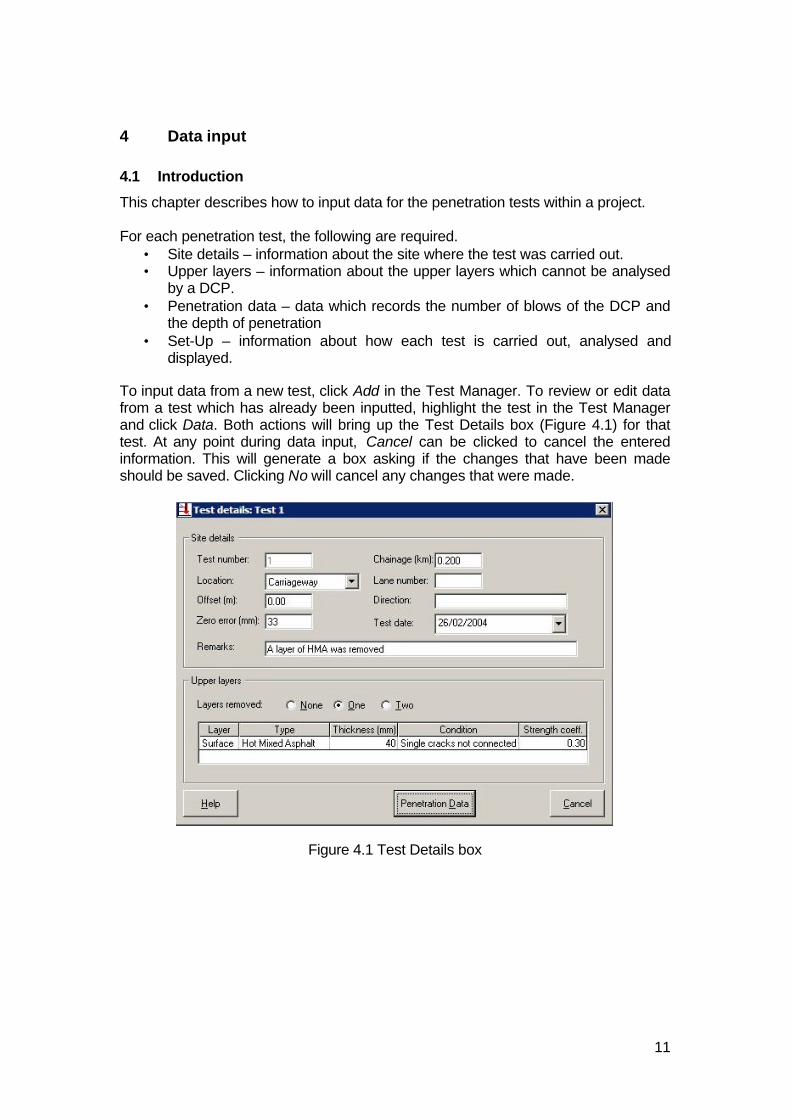
To input data from a new test, click Add in the Test Manager. To review or edit datafrom a test which has already been inputted, highlight the test in the Test Managerand click Data. Both actions will bring up the Test Details box (Figure 4.1) for thattest. At any point during data input, Cancel can be clicked to cancel the enteredinformation. This will generate a box asking if the changes that have been madeshould be saved. Clicking No will cancel any changes that were made.

Figure 4.1 Test Details box

12

4.2 Site details

The top panel of the Test Details box is titled Site details and records informationabout the site where the test was carried out. The panel has a number of fields.These are mandatory (M), optional (O) or filled in automatically (A).

Testnumber

A This field is filled in automatically according to the chainage andlocation of the test, as described in 3.2 above.

Chainage(km)

M It is important that all tests within a project use the same chainagedatum.

Location M Although penetration tests are normally carried out in thecarriageway of a road, it may be necessary to measure the strengthof the construction off the carriageway line. When results areanalysed, it will be necessary to distinguish between these locationsso that, for example, carriageway improvement works are notdesigned using layer strengths measured in a soft verge. Therefore,using the pull-down menu, select the location of the test fromcarriageway, shoulder, verge and lay-by / other. Carriageway is thedefault location.

Lanenumber

O It may be necessary to record in which lane of a road a test wasmade. Thus this field may be required if tests are being carried outon a road with more than one lane in each direction. Any normal localconvention can be used for numbering lanes.

Offset(m)

O This refers to the offset from a datum line along the road. It is normalto use the carriageway edge as the datum, although the centre line ofthe road could be used instead.

Direction O This is the traffic direction of the lane where the tests are beingcarried out. Direction does not need to be recorded on a single laneroad. The field is limited to 25 characters.

Zeroerror(mm)

M The zero error is the reading on the vertical scale of the DCP whenthe cone is sitting on a flat surface and is a result of the way in whichthe instrument is manufactured and assembled. The zero error ismeasured by placing the DCP on a smooth, level, hard surface,lowering the cone to the surface and reading the scale. This shouldbe done whenever the DCP is prepared for use and, ideally, beforeevery new series of tests. The zero error should be entered for everytest.

Test date M This defaults to today’s date, but can be changed using the pull downcalendar.

Remarks O These can be either typed or copied and pasted as required. Thefield is limited to 60 characters.

If the details of a test have already been entered, click Edit to be able to makechanges, although if the data has already been analysed, a box will be generatedwarning that editing the data will delete this analysis.

13

4.3 Upper layers

UK DCP uses penetration data to calculate the strength of most pavement layers.However, some layers are too thin, strong or impenetrable for relationships betweenpenetration rate and strength to be derived. In this case, the strength of the layer isassessed from the type of the layer and its condition. This applies to layer types suchas:

Surface• Thin bituminous seal• Hot mix asphalt• Concrete• Other surface

Base• Cement treated base• Bituminous base• Coarse granular base (such as Water Bound Macadam)

Since these layers are always found at the top of a pavement, they are referred to asUpper Layers. Layers whose strength can be calculated from penetration data arereferred to as Test Layers.

The calculation of layer and pavement strength for Upper layers and Test layers isexplained in detail in 6.1 below.

The bottom panel of the Test Details box (Figure 4.1) is titled Upper layers. Aselection must be made and a table must be completed.

4.3.1 Layers removed

Although Upper layers such as a thin bituminous seal can be penetrated by a DCP,some layers, such as hot mix asphalt or a cement treated base cannot bepenetrated. It is necessary to remove these layers by drilling or cutting out before thetest can be carried out. When inputting data, the number of upper layers which wereremoved should be entered. UK DCP can accept the removal of 0, 1 or 2 layers. Ifmore than two have been removed, it is necessary to group them into two or fewerremoved layers. Figure 4.2 illustrates the differences between Upper layers, Testlayers and removed layers for a variety of pavement constructions.

14

Pavement a) is unpaved. All layers can be analysed using penetration data. In this respectthere are no Upper layers, although in subsequent stages, such as the SNCalculation box, described in 6.2 below, and the Penetration Data Report, describedin 9.2.1 below, Unpaved will be recorded as an Upper layer so that the user isreminded of the surface type.

Pavement b) has a thin bituminous seal over a granular base. The thin seal cannot beanalysed using penetration data and is therefore an Upper layer. Since the materialcan be penetrated by a DCP cone, it is not necessary to remove the layer. Thereforefor this test there is one Upper layer but it is not removed.

Pavement c) has an HMA surface over a granular base. The HMA cannot be analysed usingpenetration data and is therefore an Upper layer. The material cannot be penetratedby a DCP cone and so must be removed. Therefore for this test, there is one Upperlayer and it is removed.

Pavement d) has a concrete surface over a granular base. As for pavement c), the concreteis an impenetrable Upper layer and must be removed. However, rigid pavements arenot analysed using Structural Numbers and therefore, although UK DCP calculatesthe Structural Numbers, only the strengths of the individual Test layers can be used.

Pavement e) has an HMA surface over a base such as water bound macadam. Both layersare impenetrable. Therefore for this test, there are two Upper layers and both areremoved.

Figure 4.2 Illustration of Upper layers, Test layers and Removed layers

4.3.2 Upper layer details

For each Upper layer, the following information must be entered into the table.

Layer This will be prompted according to the number of layers which have beenremoved. If 0 or 1 Upper layers have been removed, only one layer will beprompted and will be defined as Surface. If two Upper layers have beenremoved, two layers will be prompted. The first will be defined as Surface andthe second as Base.

Type Options will be offered from the list in 4.3 according to whether the layer is asurface or a base and whether or not the layer has been removed. If no Upperlayers have been removed, Unpaved will also be offered as an option. Graveland earth surfaces can be analysed using penetration data and so are nottechnically Upper layers, but will be recorded as such so that the surface typewill be listed when reports are generated. If the layer is Unpaved, the final threecolumns are automatically left grey and inactive since the layer will be analysedusing penetration data rather than condition. If the layer is concrete, the final two

Unpaved

UpperLayers

TestLayers

ThinBituminous

SealHMA

One layerremoved

No layers removed

HMA

Base

Two layersremoved

a) b) c) d)

Concrete

e)

15

columns are automatically left grey and inactive since rigid pavements are notanalysed using Structural Numbers.

Thickness(mm)

Thicker layers contribute more strength to the pavement. UK DCP will generatea prompt if the value is too high or low for that type of layer. If the layer is a thinbituminous seal, a default thickness of 20 mm will be automatically entered. Box4.1 provides guidance on how to record the removal of very thick Upper layers.

Condition The observed condition of a surface layer is used to determine its strengthcoefficient. If the condition is known, use the pull down menu to select acondition. Then click in the strength coefficient box and the value will be enteredautomatically. If condition is unknown, or it is already known which strengthcoefficient to use, enter a condition of ‘Unknown’ and then manually enter thevalue. If there are two Upper layers, it is often difficult to assess the condition ofthe base. Therefore a condition of Unknown is automatically generated for thebase and the strength coefficient must be entered manually.

Strengthcoefficient

The strength coefficient is required to calculate the contribution of the layer to thestrength or Structural Number of the pavement. It can be entered manually orgenerated automatically from the condition of the layer. If it is entered manually,UK DCP checks that it is within a realistic range for the layer type selected.

Box 4.1 Recording the removal of very thick Upper layers

UK DCP can be used to analyse granular layers underneath thin or thick bituminoussurfacing. The maximum allowable thickness of HMA or bituminous layer is 350 mm sincethis is a normal upper limit for this material type. However, if a greater thickness of asphalt isremoved before the DCP can be used, it is recommended that it is recorded in two layers; asurface layer of HMA with its observed condition and automatically generated strengthcoefficient followed by a base layer of bituminous material with unknown condition and astrength coefficient manually entered to be equal to that of the surface layer. The maximumtotal thickness of the removed asphalt is therefore 700 mm which should be sufficient for allroads.

There are five buttons below the Upper Layer panel.

Help Open this manual on the screen at the appropriate section.

PenetrationData

Open a Penetration Data box so that test data can be entered.Clicking this button also checks that all data entered into theTest Details box is valid. Any invalid entries must be correctedbefore the Penetration Data box can be opened.

Cancel Close the box and return to the Test Manager without savingthe changes that have been made since the box was created oropened for editing. A box is generated seeking confirmationthat the changes should be saved.

Edit Edit the data in the box. If the current data has already beenused to identify layers, a box will be generated warning thatediting the data will delete this analysis.

Close

Visible ifdata hasalready beenentered andsaved Return to the Test Manager without making any edits.

16

4.4 Penetration data

After completing the Test Details box with Site details and Upper layer information,click Penetration Data to open an empty Penetration Data box. This box has twopanels.

Figure 4.3 Penetration Data box (with test data)

4.4.1 Site details summary

This panel provides a summary of the site details which have already been entered.These details cannot be edited.

4.4.2 Penetration data

During a DCP test, the cone is driven into the pavement under repeated blows. Therecord from a test consists of a number of test points. At each test point the numberof blows since the last test point is recorded and the total penetration of the cone ismeasured.

It is recommended that the penetration of the cone should be measured atincrements of about 10 mm. However, it is usually easier to measure penetrationafter a set number of blows. It is therefore necessary to change the number of blowsbetween measurements according to the strength of the layer being penetrated. Forgood quality granular bases, measurements every 5 or 10 blows are normallysufficient, but for weaker sub-bases and subgrades, measurements every 1 or 2blows may be required. There is no disadvantage in taking too many readings but iftoo few are taken, there is a danger that weak spots will be missed and layerboundaries will be difficult to identify.

17

This data is entered into the table in this panel. Each row in the table represents onetest point. The table has four columns.

Pointnumber

The number of each test point. If a point is inserted or deleted, the numbering isautomatically corrected. A maximum of 250 test points can be entered for eachDCP test. If more than 250 have been recorded, it is likely that the cone hit animpenetrable object such as a stone, in which case the data is of no use.

Blows The number of blows given to the cone to drive it from the previous point to thecurrent point. The number of blows at the first test point is automatically set atzero. A maximum of 25 blows are permitted between each test point. If moreblows are given, changes in depth are likely to be too high for useful results tobe calculated.

Penetrationdepth (mm)

The depth at the current point, as read off the DCP scale. The depth of the firsttest point, the ‘initial reading’, is recorded before any blows have been given.Since the zero error (see above) is measured when the DCP is placed on asmooth and level surface, it is impossible for the initial reading to be less thanthe zero error. The initial reading also includes the thickness of all removedlayers. It will not be accepted if it is less than the sum of the zero error and thethicknesses of the removed layers as if so, it is likely to be an error. Note that inFigure 4.3 the initial reading (78) is greater than the sum of the zero error (33)and the thickness of the removed layer (40). A maximum penetration depth of1500 mm is allowed. If the cone has penetrated further than this, it is likely thatfriction along the rod is significantly reducing the penetration rate of the cone, inwhich case the data is unreliable and should not be used.

Comments Comments are entered automatically if an impenetrable layer was drilled or ifan extension rod was used (see below).

Box 4.2 Calculating adjusted penetration data

In order to analyse a penetration test, two corrections to the recorded depths are necessary.• The zero error is subtracted from all depths.• The length of an extension rod (see below), where used, is added to the depths of all test

points recorded after the rod was fitted.UK DCP makes these corrections automatically. The corrected data is referred to as‘adjusted data’.

To the right of the table are three buttons. These are used when entering or deletingpenetration data.

Insert Insert a test point into the data. Highlight the row below which the new test isrequired and click Insert. Then enter the data from the new test point into the emptyrow.

Delete Delete a test point. Highlight the test point to be deleted and click Delete. The firsttest point cannot be deleted.

Paste This button is used to transfer the penetration data of one test from a spreadsheetinto the panel, for example if the data was entered on site into a palm top or otherdevice. The data should be entered into the spreadsheet in two columns:incremental blows and total depth (mm). Highlight and copy the two columns. Thenreturn to UK DCP and click Paste. It is not necessary to position the cursor in thefirst row before clicking Paste.

18

Penetration data can also be entered manually. On the first row type the penetrationdepth before any blows have been given and then use Tab or Enter on the keyboardto enter data in one cell after another.

There are six buttons below the table.

Help Open this manual on the screen at the appropriate section.

TestDetails

Return to the Test Details box.

OK Save the data entered into the Test Details and Penetration Databoxes and return to the Test Manager. If the test was a new test,a further Test Details box will be generated. If the test had beenentered earlier and the data was being reviewed or edited, afurther box is not generated.

Cancel Close the box and return to the Test Manager without saving thechanges that have been made since the box was created oropened for editing. A box is generated seeking confirmation thatthe changes should be saved.

Edit Edit the penetration data. If the current data has already beenused to identify layers, a warning will be generated that editingthe data will delete this analysis.

Close

Visible ifdata hasalreadybeenenteredand saved

Return to the Test Manager without making any edits.

19

A comment will be entered automatically if a layer was drilled or an extension rodwas used.

Drilled layer

If an impenetrable layer has been drilled, the penetration data will include one pointrecorded before the DCP was removed and another point recorded after the layerwas drilled. There will be a difference in depth between these points, although noblows will have been recorded. If this data is pasted from a spreadsheet, a commentwill automatically appear in the Comment column stating ‘Layer Drilled’ (see Figure4.4). If data is edited or a point is inserted or deleted to give a depth difference withno recorded blows, a prompt will ask if a layer has been drilled. If Yes is clicked, thesame comment is entered; if No is clicked, the Blows entry is deleted and should bere-entered. Drilled layers are recorded and presented in later stages of the analysis.Only one drilled layer can be recorded in a test. If two layers were drilled to achievethe desired penetration depth, it is likely that the material was excessively disturbed,in which case the data is unreliable and should not be used.

Extension rod

In normal operation, a DCP can penetrate to 800 mm. It is possible to add anextension rod to allow the DCP to penetrate further. In this case, one point will berecorded before the DCP was removed and another after the extended DCP wasreinserted. The second point will have a numerically lower reading than the first, andno blows will have been recorded. If this data is pasted from a spreadsheet, acomment will automatically appear stating ‘Extension Rod Added’ (see Figure 4.4). Ifdata is edited or a point is inserted or deleted to give a point with no blows and anapparent reduction in depth, a prompt will ask if an extension rod has been added. IfYes is clicked, the same comment will appear; if No is clicked, the Blows entry isdeleted and should be re-entered. UK DCP will take account of the use of anextension rod, determine the length of the rod from the difference between the twodepth readings and adjust the penetration data accordingly. If there is an apparentreduction in depth before 400 mm of penetration has been reached, the prompt willnot be generated since it is unlikely that an extension rod was added when depthswere small. A reduction in depth before 500 mm is probably due to an error in thedata and an error message will be generated. Only one layer can be recorded asbeing due to the use of an extension rod since if further extension rods are used, it islikely that friction along the rod is significantly reducing the penetration rate of thecone, in which case the data is unreliable and should not be used.

20

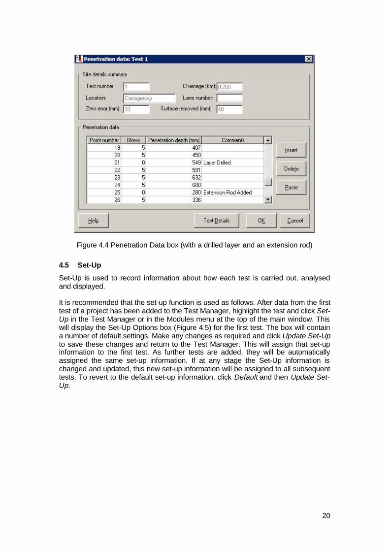
Figure 4.4 Penetration Data box (with a drilled layer and an extension rod)

4.5 Set-Up

Set-Up is used to record information about how each test is carried out, analysedand displayed.

It is recommended that the set-up function is used as follows. After data from the firsttest of a project has been added to the Test Manager, highlight the test and click Set-Up in the Test Manager or in the Modules menu at the top of the main window. Thiswill display the Set-Up Options box (Figure 4.5) for the first test. The box will containa number of default settings. Make any changes as required and click Update Set-Upto save these changes and return to the Test Manager. This will assign that set-upinformation to the first test. As further tests are added, they will be automaticallyassigned the same set-up information. If at any stage the Set-Up information ischanged and updated, this new set-up information will be assigned to all subsequenttests. To revert to the default set-up information, click Default and then Update Set-Up.

21

Figure 4.5 Set-Up Options box

If a number of tests have been added to the Test Manager, or even if analysis of thedata has already begun, it is possible to return to the Test Manager and change theSet-Up information for a single test. This may be done if a chosen method of analysisor display is unsuitable for the data. Highlight the test, click Set-Up, make therequired changes and click Update Set-Up. If analysis of that test has already beencarried out, a box is generated warning that the analysis will be deleted. It should benoted that if more tests are added, they will retain this updated Set-Up information.

There are four buttons in the Set-Up Options box.

Help Open this manual on the screen at the appropriate section.

Default Revert to the default set-up information, as defined below.

Update Set-Up Save amended set-up information, as described above.

Cancel Close Set-Up and return to the Test Manager without saving any changes.

The Set-Up Options box has four panels.

4.5.1 Analysis

Layers can be identified either automatically by UK DCP or manually by the user.This panel allows the method of identification to be selected. The default is automatic(‘system’) analysis.

4.5.2 Sectioning

A project can be divided into sections either automatically by UK DCP or manually bythe user. This panel allows the method of identification to be selected. Automaticsectioning is currently disabled. The default is manual (‘user’) sectioning.

22

4.5.3 CBR Calculation

The strengths of Test layers are calculated by converting the penetration rate (mmper blow) to a California Bearing Ratio (CBR) value and then from the CBR value toa strength coefficient and finally to a Structural Number. A number of relationshipsbetween penetration rate and CBR value have been derived and are given in Table4.1. Some of these are used when the DCP cone has an angle of 60°, others whenthe cone has an angle of 30°. The relationship and the cone angle are selected onthis panel. The user’s organisation should provide guidance as to which relationshipshould be used or whether a new relationship for the local conditions should bedeveloped. The default is the TRL relationship for a 60° cone.

The conversion of CBR value to strength coefficient and Structural Number isdescribed in Chapter 6.

Table 4.1 Penetration rate – CBR relationships

Coneangle

Name of relationship Relationship

60°cone

TRL(1) Log10(CBR) = 2.48 – 1.057 Log10(pen rate)

Kleyn(2) (pen rate > 2mm/blow)

CBR = 410 (pen rate)-1.27

Kleyn(3) (pen rate = 2mm/blow)

CBR = 66.66 (pen rate)2 – 330 (pen rate) + 563.33

Expansive ClayMethod(4)

Log10(CBR) = 2.315 – 0.858 Log10(pen rate)

100% Planings (5) Log10(CBR) = 1.83 – 0.95 Log10(pen rate)

50% Planings Log10(CBR) = 2.51 – 1.38 Log10(pen rate)

User-Defined Log10(CBR) = [constant] – [coefficient] Log10(pen rate)

Constant and Coefficient can be defined by the user

30°cone

Smith and Pratt(6) Log10(CBR) = 2.555 – 1.145 Log10(pen rate)

User-Defined Log10(CBR) = [constant] – [coefficient] Log10(pen rate)

Constant and Coefficient can be defined by the user

(pen rate is the penetration rate measured in millimetres per blow)

23

4.5.4 Other Options

When penetration data is being analysed, a graph of penetration depth against thenumber of blows given to the DCP is used to identify layers of different materials andthe boundaries between them. The items in this panel allow two changes to be madeto this graph which may help in identifying layers.

As-Built Thickness

It is sometimes difficult to identify layers from a penetration graph and, even if layerscan be seen, it can be difficult to be sure whether the layer is part of the base, sub-base or subgrade. If actual information on materials and layer thicknesses isavailable, layer identification from penetration data can be much easier. Thisinformation can come from records made when the pavement was being constructedor from test pits dug alongside and within the project. Neither source of informationwill accurately predict the layers at each test site, but they can provide usefulguidance. If as-built or test pit information is available, click in the As-Built ThicknessKnown? box and enter the recorded thicknesses for the Surface, Base and Sub-base. These will be displayed on the penetration graphs, as shown in, for example,Figure 5.2 and Figure 5.4. The default is to not display as-built thicknesses.

Colours

Different colours are used to indicate different elements of the penetration graph.They can be changed if required, for example if a printer does not print a particularcolour well. The defaults are Data Point – dark green; Test Layers – dark blue;underside of Upper Layers – bright blue; Drilled Layer – red.

After data from penetration tests has been input, the Test Manager is as shown inFigure 4.6.

Figure 4.6 Test Manager (showing that test data has been input)

24

5 Layer analysis

5.1 Introduction

A typical graph of penetration depth against the cumulative number of blows given tothe DCP shows a line of varying gradient. The gradient is equal to the penetrationrate of the cone as it is driven into the pavement.

For Test layers, it is possible to derive relationships (4.5.3) between the penetrationrate and the strength of the material through which the cone is passing. The gradientof the line can therefore be used to calculate the material strength. Changes in thegradient of the line indicate boundaries between materials of different strengths andhence the thicknesses of layers of different strengths.

Upper layers are often too thin, strong or impenetrable for their strength to bedetermined from the penetration rate. Instead, the strength of an Upper layer isestimated from the type of the layer and its condition, and its thickness is taken fromas-built records, test pit data or by measuring the thickness of a layer removedduring the DCP test.

This chapter describes how the thicknesses of Test layers are determined frompenetration graphs; Chapter 6 then describes how the strengths of Upper layers andTest layers are calculated.

The penetration graph can be analysed automatically or manually according to theselection made when defining Set-Up information (4.5.1).

5.2 Analysing Test layers

Begin layer analysis from the Test Manager. Highlight a test which has not yet beenanalysed and click Analyse in the Test Manager or in the Modules menu at the top ofthe main window.

This will open a Layer Boundaries box. It contains a graph of adjusted penetrationdepth (data adjustment is explained in Box 4.2) against the cumulative number ofblows given to the DCP. All test points are plotted onto the graph. The gradient of theline of test points is the penetration rate of the cone and hence the strength of thematerial at that depth. A shallow gradient indicates strong material, a steep gradientindicates weak material and changes in gradient indicate a layer boundary betweenTest layers of different strengths.

The other information displayed on the graph depends upon whether layer analysiswill be carried out automatically or manually. These two alternatives are compared inBox 5.1 and described in detail below.

25

Box 5.1 Should penetration data be analysed automatically or manually?

UK DCP allows penetration plots to be analysed automatically or manually. Each method hasadvantages and disadvantages.

Automatic analysis

AdvantagesQuicker than manual analysis.

DisadvantagesThe user has no control over where layer boundaries are located.Assigns a strength coefficient to a drilled layer.

SummaryAutomatically identified layer boundaries of a complex plot may be located inappropriately.Automatic analysis is therefore recommended when the penetration plot has a simple shape.

Manual analysis

AdvantagesUser has more control over where layer boundaries are located.The use of gaps can improve the analysis of drilled and strong layers.

DisadvantagesSlower than automatic analysis.

SummaryManual analysis is recommended when the penetration plot has a complex shape, theanalysis of which the user would like to have some control over. It is also recommended if anatypical item such as a large stone slowed down the penetration or had to be drilled.

5.3 Automatic layer analysis

The automatic layer analysis procedure first calculates the penetration rate at eachtest point and the average penetration rate for the entire test. For each test point itthen calculates the value of the average rate minus the rate at that point. Thesevalues are then summed in turn starting at the first test to find the cumulativedifference sum at each point. By the nature of the calculation, this sum will be zero atthe final test point. At one point this sum will reach a maximum absolute value. Thedepth of the point at which the sum reaches this maximum value is defined as thefirst Test layer boundary. This procedure has a similar effect to drawing a straightline from the first point to the last point and finding the depth of the intermediate pointwhich is furthest from this straight line (as shown in Figure 5.1).

26

Figure 5.1 How Automatic analysis works

The procedure is then repeated for the test points above this first boundary and forthe points below it. In this way the second and third boundaries can be identified.The procedure is repeated until the points between any two boundaries do notexhibit sufficient fluctuation from a straight line to allow a further boundary to beidentified with any degree of confidence. An automatically analysed penetration plotis shown in Figure 5.2.

Figure 5.2 Layer Boundaries box using Automatic layer analysis

27

To illustrate automatic layer analysis, Table 5.1 contains penetration data to a depthof 225 mm. The data is analysed in the table to show how a change from strong toweaker material can be identified at a depth of 75 mm. Figure 5.1 contains a graph ofthe data in this table. It shows how the point with the greatest cumulative differencesum is also the point which lies furthest from a straight line from the first point to thelast point. The first Test layer boundary has been automatically generated and isshown on the graph.

Table 5.1 Example of penetration data and cumulative difference sum analysis

Point Blows Adjusted pendepth

Pen rate(mm/blow)

Av. Penrate

Av. Pen rate –pen rate

Cumulativedifference sum

1 0 02 5 14 2.8 4.5 1.7 1.73 5 29 3.0 4.5 1.5 3.24 5 46 3.4 4.5 1.1 4.35 5 62 3.2 4.5 1.3 5.66 5 75 2.6 4.5 1.9 7.5 ? maximum value7 5 107 6.4 4.5 -1.9 5.68 5 133 5.2 4.5 -0.7 4.99 5 164 6.2 4.5 -1.7 3.210 5 196 6.4 4.5 -1.9 1.311 5 225 5.8 4.5 -1.3 0

Five points should be noted when using automatic layer analysis.• Boundaries can be identified only at depths corresponding to actual test

points.• The strength of a layer is calculated by the gradient of a straight line from the

intersection of its upper boundary with the line of test points to theintersection of its lower boundary with the line of test points.

• There are three situations where minor corrections are made to the analysisin order to prevent inaccurate calculation of the thickness of the first Testlayer. These are described in Box 5.2.

• Box 5.3 below recommends when automatic layer analysis should be usedfor penetration data containing drilled layers.

• Box 5.4 below recommends when automatic layer analysis should be usedfor penetration data containing strong but penetrable layers.

The following items are displayed in the Layer Boundaries box if automatic layeranalysis has been selected. The colours of some of the items depend upon selectionmade when defining Set-Up information.

Maximumlayersmessage

When the box is opened, a message will be generated giving the maximumnumber of Test layers which can be identified from the data using the aboveprocedure. Click OK to delete this message. If 10 Test layers can be identified(the limit set by UK DCP), a message is not generated.

First layerboundary

The first layer boundary identified using the above procedure is shown with ahorizontal line.

Number ofLayers field

The number in this box is the number of Test layers currently being shown.Clicking the Up and Down arrows increases and decreases this number andadds or removes layer boundaries from the graph. The number can beincreased up to the number which was shown in the Maximum layers

28

message. Unless a drilled layer is present, this number is initially 2.

Upper layerline

A dashed line indicates the underside of the Upper Layers.

Drilledlayers

If a layer has been drilled, it will be marked on the graph with two horizontaldotted lines, but the first automatic layer will not be shown. The Number ofLayers field will therefore initially show 3, the portion above the drilled layer,the drilled layer itself and the portion below. An automatically analysed drilledlayer is shown in Figure 5.12 below.

As-builtlayers

If as-built or test pit information was entered into the Set-Up of the test (4.5.4),these layers are shown, separated by dotted lines.

ShowGridlines

A check box is provided to allow gridlines to be displayed or removed.

AdjustedData button

Click this button to generate a box showing the penetration data (Figure 6.3).This data has been adjusted as described in Box 4.2. The box also includesthe average penetration rate between successive points. This box isgenerated to guide the identification of Test layers and cannot be edited.

Help button This button opens this manual on the screen at the appropriate section.

OK button This is used to accept and save the layer boundaries and return to the TestManager.

Cancelbutton

This is used to cancel the analysis. If changes have been made to theanalysis, a box is generated which offers an opportunity to save the changes.

Layerdescriptions

When the cursor is placed over the graph, a small box is generated. This boxgives the number of the Test layer, its thickness (mm) and the averagepenetration rate for the layer.

Pointdescriptions

When the cursor is placed over a test point, a small box is generated. Thisbox gives the cumulative blows and the adjusted depth of the point.

Add or remove layer boundaries from the graph until satisfied that the data has beenadequately analysed. In Figure 5.2 five Test layers appear sufficient. Adding furtherlayers does not increase the precision of the analysis. Note that identified Test layersmatching previously defined as-built layers is a useful check on the analysis.

Click OK to save the analysis and return to the Test Manager. It will be seen (Figure5.3) that today’s date will be in the Analysis column for that test.

Figure 5.3 Test Manager (showing that test data has been analysed)

29

It is possible to examine the graph and possibly edit the analysis of a test for whichlayers have already been identified. Highlight the test in the Test Manager and clickAnalyse. The Layer Boundaries box will be opened and the penetration graph will beshown, but Edit must be clicked before changes can be made to the number of Testlayers. When Edit is clicked, if SN Calculations have already been carried out, awarning appears that SN Calculation data, and possibly Sectioning data will bedeleted. If it is not necessary to edit the analysis, click Close to return to the TestManager.

Box 5.2 Corrected analysis of deep surface texture and disturbed soil

There are three situations where automatic layer analysis makes assumptions about theadjusted penetration data (adjusted penetration data is explained in Box 4.2) and makesminor corrections in order to prevent the inaccurate calculation of the thickness of the firstTest layer. These three situations are described below. In each case, it is important tounderstand how a simple automatic routine without these assumptions or a manualinterpretation of the penetration graph would produce the inaccuracy.

1. If an earth, gravel or thin bituminous surface has a deep texture or surface voids, the initialposition of the DCP cone may be slightly below the actual road surface. UK DCP assumesthe road surface to be at an adjusted penetration of zero and calculates the layer strengthfrom the penetration rate after penetration began.

2. If base material sticks to an impenetrable layer as it is removed, as is often the case withHMA and a granular base, the initial position of the DCP cone may be below the actual topsurface of the base. UK DCP assumes the top surface of the base layer to be at an adjustedpenetration equal to the measured thickness of the removed layer and calculates the layerstrength from the penetration rate after penetration began.

3. If base material is loosened by an impenetrable layer as it is removed, the first one or twoblows to the DCP will penetrate much more quickly through the loose material than laterblows in the unloosened material. UK DCP ignores the penetration rate in the loose material,assumes the top surface of the base layer to be at an adjusted penetration equal to themeasured thickness of the removed layer and calculates the layer strength from thepenetration rate below the loose material.

As a result of point 3, it is recommended that after a layer has been removed, the first twopenetration readings are taken after only one or two blows.

5.4 Manual layer analysis

Test layer boundaries are identified as follows. UK DCP allows a number of straightlines to be drawn along approximately straight portions of the graph. Test layerboundaries will be generated at each point where these lines intersect. A manuallyanalysed penetration plot is shown in Figure 5.4.

30

Figure 5.4 Layer Boundaries box using Manual layer analysis

Four points should be noted when using manual layer analysis.• Boundaries can be identified at any depth at which lines intersect.• The strength of a layer is calculated by the gradient of the straight line drawn

onto the plot. Various techniques allow the user more control over layerthickness than is possible with automatic layer analysis. These are describedbelow.

• Box 5.3 below recommends when manual layer analysis should be used forpenetration data containing drilled layers.

• Box 5.4 below recommends when manual layer analysis should be used forpenetration data containing strong but penetrable layers.

31

The following items are displayed in the Layer Boundaries box if manual layeranalysis has been selected. The colours of some of the items depend upon selectionmade when defining Set-Up information.

Number ofLayers field

The number in this box is the number of Test layers identified. As a newinteresting straight line is drawn, the number in this field increases by one.

Upper layerline

A dashed line indicates the underside of the Upper Layers.

Drilledlayers

If a layer has been drilled, it will be marked on the graph with two horizontaldotted lines.

As-builtlayers

If as-built or test pit information was entered into the Set-Up of the test (4.5.4),these layers are shown, separated by dotted lines.

ShowGridlines

A check box is provided to allow gridlines to be displayed or removed.

Zoom box A pull down menu allows the graph to be magnified so that lines can be moreaccurately placed.

AdjustedData button

Click this button to generate a box showing the penetration data (Figure 6.3).This data has been adjusted as described in Box 4.2. The box also includesthe average penetration rate between successive points. This box isgenerated to guide the identification of Test layers and cannot be edited.

Add Linebutton

Click this button to draw a straight line. Then click and hold at one end of theintended line. Drag the cursor to the end of the intended line and release.Double click on a line to delete it.

DisplayLayersbutton

Click this button to generate layer boundaries where the straight linesintersect. After layer boundaries have been generated, an additional straightline can be added, allowing the user to be satisfied with the analysis of aportion of the graph before completing the analysis. As the new line is drawn,the previously generated layer boundaries disappear.

RemoveLayersbutton

Click this button to remove all straight lines and layer boundaries.

Help button This button opens this manual on the screen at the appropriate section.

OK button This is used to accept and save the layer boundaries and return to the TestManager.

Cancelbutton

This is used to cancel the analysis. If changes have been made to theanalysis, a box is generated which offers an opportunity to save the changes.

Layerdescriptions

When the cursor is placed over the graph, a small box is generated. This boxgives the number of the Test layer, its thickness (mm) and the averagepenetration rate for the layer.

Pointdescriptions

When the cursor is placed over a test point, a small box is generated. Thisbox gives the cumulative blows and the adjusted depth of the point.

32

Study the graph and model it as a series of straight lines. Click Add Line and drawlines along each reasonably straight portion. These lines should form a series ofinterconnecting lines, although Gaps may be deliberately left in certain situations.Click Display Layers to generate the Test layer boundaries. In Figure 5.4 five straightlines seem to represent the graph sufficiently accurately, although an importantcheck is described below in Box 6.1. Note the closeness of the Test layers to thepreviously defined as-built layers and the similarity of the result to that derived usingautomatic analysis (Figure 5.2).

Click OK to save the analysis and return to the Test Manager. It will be seen (Figure5.5) that today’s date will be in the Analysis column for that test.

Figure 5.5 Test Manager (showing that test data has been analysed)

To edit the analysis of a test for which layers have already been identified, highlightthe test in the Test Manager and click Analyse. The Layer Boundaries box will beopened and the penetration graph will be shown, but Edit must be clicked beforechanges can be made to the number of Test layers. When Edit is clicked, if SNCalculations have already been carried out, a warning appears that SN Calculationdata, and possibly Sectioning data will be deleted. If it is not necessary to edit theanalysis, click Close to return to the Test Manager.

In most cases, manual layer identification is straightforward. However, there are anumber of hints and techniques which should be noted. They are illustrated in thefigures below.

Doubleintersections

Figure 5.6 If a graph has a sudden change of gradient, the boundary canbe identified using only two straight lines. However, if a graphhas a gradual change of gradient, three or more short lines maybe required. If these lines are drawn too long, it may occur thatone line has two or more intersections. In this case, boundariesmay be generated at unintended intersections. It isrecommended that double intersections are avoided.

Negativegradients

Figure 5.7 Since penetration graphs always have a gradient from top leftto bottom right, a line in the opposite direction will not beaccepted.

Intersectingthe line of

Figure 5.8 A line which does not cross the line of test points will not beaccepted.

33

points

Moving aline

Figure 5.9Figure 5.10

If a line does not exactly match a portion of the graph, it can bemoved laterally by clicking, holding and dragging.

Overlappinglines

Figure 5.11 If a line overlaps but does not intersect another line, a warningmessage is generated and the line is deleted.

Gapsbetweenlines

Figure 5.12

Figure 5.13

Figure 5.14

Figure 5.15

The use of non-intersecting lines can assist in the analysis ofdrilled and very strong layers. Their use is described in detail in5.5 below.

34

Figure 5.6 Double intersectionsThree straight lines have been drawn and both true intersections have been ringed.The lower intersection has been correctly identified, but the upper intersection has

been missed in favour of a false intersection. The lines should be removed bydouble-clicking and shorter lines drawn to prevent double intersections.

Figure 5.7 Negative gradientLines with negative gradient will not be accepted. After clicking OK, the line will be

deleted and should be redrawn.

35

Figure 5.8 Line does not intersect the line of test pointsStraight lines which do not cross the line of test points will not be accepted. After

clicking OK, the line will be deleted and should be redrawn.

Figure 5.9 Line drawn parallel to its intended positionNote that if the line does not cross the line of test points, it will not be accepted.

36

Figure 5.10 Line moved laterally to its intended positionThe line in Figure 5.9 has been moved and layers boundaries have been generated

at the intersections.

Figure 5.11 Lines overlap but do not intersect.Lines which overlap without intersection will not be accepted. After clicking OK, the

line will be deleted and should be redrawn.

5.5 Analysis of drilled and very strong layers

If two manually drawn lines do not intersect, the boundary will be generated at adepth midway between the two end points. Drawing non-intersecting lines can beuseful in the analysis of a drilled layer, a very strong but penetrable layer or anobstacle such as a stone.

The following figures and boxes describe how these examples are analyseddifferently under automatic and manual analysis and how the most appropriatemethod should be chosen.

37

5.5.1 Drilled layers

Figure 5.12 Automatic analysis of a drilled layer

38

When analysed automatically, the drilled layer is defined as a distinct Test layer.Later, during the calculation of Structural Numbers, a strength coefficient will have tobe manually assigned to this layer. In Figure 5.12 four Test layers have beenidentified, one of them the drilled layer.

Figure 5.13 Manual analysis of a drilled layer and the use of gaps

When analysed manually, the drilled layer is not defined as a distinct Test layer. Aboundary can be identified in the middle of the drilled layer. This is done byterminating the drawn lines at the upper and lower surfaces of the drilled layer andso generating a boundary midway between the two end points. The strengths of thetwo layers are calculated from the gradients of the drawn lines, thus eliminating theinfluence of the drilled layer on the analysis. In Figure 5.13 only three Test layershave been identified, the thickness of the drilled layer being divided equally betweenbase and sub-base.

Box 5.3 Analysis of a drilled layer

Automatic analysis identifies a drilled layer as distinct and assigns a strength coefficient.Manual analysis with the use of gaps can eliminate the influence of the drilled layer on thesubsequent analysis. Therefore automatic analysis should be used when, for example, astrongly stabilised pavement layer had to be drilled, while manual analysis should be usedwhen an isolated and atypical item such as a large stone had to be drilled.

39

5.5.2 Very strong layers

Figure 5.14 Automatic analysis of a very strong layer

When analysed automatically, the very strong but penetrable layer is likely to bedefined as a distinct Test layer. Later, during the calculation of Structural Numbers, ahigh strength coefficient will be assigned to this layer. In Figure 5.14 four Test layershave been defined, one of them the very strong layer.

40

Figure 5.15 Manual analysis of a very strong layer and the use of gaps

When analysed manually, the very strong but penetrable layer does not have to bedefined as a distinct Test layer. A boundary can be identified in the middle of thestrong layer. This is done by terminating the drawn lines at the upper and lowersurfaces of the strong layer, generating a boundary midway between the two endpoints. The strengths of the two layers are calculated from the gradients of the drawnlines, thus eliminating the influence of the very strong layer on the analysis. In Figure5.15 only three Test layers have been identified, the thickness of the very stronglayer in this case being allocated to the sub-base.

Box 5.4 Analysis of a very strong but penetrable layer

Automatic analysis identifies a very strong but penetrable layer as distinct layers. Manualanalysis with the use of gaps can eliminate the influence of this layer on the subsequentanalysis. Therefore automatic analysis should be used when a very strong layer is known tobe present within the pavement, while manual analysis should be used when it is likely that astone caused an obstruction to the cone.

41

6 Structural Number calculation

6.1 Introduction

Assessing the strength of a pavement is difficult. Most pavements have severallayers and for each one many different characteristics can be measured: thickness,modulus, CBR and so on. These values can be combined in many different ways.The concept of a Structural Number (7) (SN) was developed during the AASHO RoadTest research as a single number which would indicate the strength and durability ofan entire pavement and which would be internationally recognised. The concept wasdeveloped for the analysis of flexible pavements; rigid pavements are not analysedusing Structural Numbers.

Over time, the concept has expanded. The original term, SN, was calculated fromthe imported surface, base and sub-base layers. The modified Structural Number (8)

(SNC) was then introduced to include the effect of the subgrade. However, it wasrealised that because the subgrade contribution to SNC is independent of its depth,redefining subgrade material as sub-base gives a higher SNC. Tests were carriedout and the adjusted Structural Number (9) (SNP) was developed. This adjusts thecontribution of the sub-base and subgrade according to their depth and eliminatesthis potential source of error.

This chapter describes how to calculate the Structural Number of each pavementlayer. It provides the equations used to calculate SN and SNC, although those usedto calculate SNP are too extensive to be included here.

6.1.1 Upper layers

Upper layers are layers at the top of the pavement which are too thin, strong orimpenetrable for relationships between penetration rate and strength to be derived.The contribution of an Upper layer to the Structural Number of a pavement is itsstrength coefficient multiplied by its thickness. The strength coefficient is assessedfrom the type of the layer and its condition, as described in 4.3.2 above.

6.1.2 Base and Sub-base Test layers

The contribution of a Base and Sub-base layer to the Structural Number of apavement is its strength coefficient multiplied by its thickness.

SN = S aidi

where: i is a summation over layersai is a strength coefficient for each layerdi is the thickness of each layer measured in inches

The strength coefficient of a layer can be calculated from its CBR value, which iscalculated from the penetration rate as described in 4.5.3 above.

The relationship between CBR and strength coefficient depends upon the layer andthe material. These relationships are given in Table 6.1.

42

Table 6.1 CBR – Strength Coefficient (a) relationships

PavementLayer

Relationship

Base a = 0.0001 [29.14 (CBR) – 0.1977 (CBR)2 + 0.00045 (CBR)3]

This relationship is also used for a gravel or earth surface layer (10).

Cementtreatedbase

CBR >70%

a = 0.00016 [29.14 (CBR) – 0.1977 (CBR)2 + 0.00045 (CBR)3]

CBR <70%

a = 0. Tests have shown that a cement treated base with a CBRless than 70 has minimal effective strength.

Sub-base a = 0.184 Log10(CBR) – 0.0444 (Log10(CBR))2 – 0.075

6.1.3 Subgrade Test layers

The contribution of the Subgrade to the Structural Number of a pavement is referredto as SNG and is calculated directly from CBR without the need for an intermediatestrength coefficient. SNG is a function of the CBR of the entire subgrade, rather thanany layers into which the subgrade can be divided. A procedure to identify the layerswhich have the greatest influence within the subgrade and derive the aggregatesubgrade CBR in a manner which reflects engineering judgement has therefore beendevised and is included in UK DCP.

The relationship between subgrade CBR and SNG is as follows.

SNG = 3.51 Log10(CBR) – 0.85 Log10(CBR)2 – 1.43

6.2 Calculating the Structural Number

Begin the Structural Number calculation from the Test Manager. Highlight a test forwhich Structural Numbers have not yet been calculated and click Calculate SN in theTest Manager or in the Modules menu at the top of the main window. This button isinactive if the selected test has not yet been analysed.

This will generate an SN Calculation box (Figure 6.1). This box has three panels andfive buttons, although the third panel is not visible until the second panel has beencompleted.

It is possible to view the results and possibly edit the analysis of a test for whichStructural Numbers have already been calculated. Highlight the test in the TestManager and click Calculate SN. The results will be shown, but Edit must be clickedbefore changes can be made. When Edit is clicked, if the project has already beensectioned, a warning appears that sectioning results will be deleted if editingcontinues.

43

Figure 6.1 SN Calculation box (before calculating SNs)

6.2.1 Upper layers

This panel displays the Upper layers as defined in 4.3 above. For each Upper layer,the information below is presented and cannot be edited. If the surface is gravel orearth, it will be recorded in this panel, but since it will be analysed as a Test layerusing penetration data, its depth, thickness and strength coefficient are automaticallyleft blank in this panel. If the surface is concrete, the strength coefficient isautomatically left blank as rigid pavements are not analysed using StructuralNumbers.

Number UK DCP can accept a maximum of two Upper layers.

Position The uppermost Upper layer is automatically defined as Surface. If asecond Upper layer is present, it is automatically defined as Base.

Type The layer type, as described in 4.3.2.

Thickness (mm) The thickness of each layer.

Depth (mm) The depth to the underside of each layer.

Strengthcoefficient

The determination of the strength coefficient of Upper layers wasdescribed in 4.3.2.

44

6.2.2 Test layers

This panel displays the Test layers as defined in 4.3 above. For each Test layer, sixitems of information are required. Four items are filled in automatically (A) and twomust be entered manually (M).

Number A Test layers are automatically numbered sequentially from 1.

CBR (%) A This is calculated from the penetration rate using the selectedrelationship as described in 4.5.3, although if a drilled layer isidentified as being in the subgrade, the CBR value must be enteredmanually.

Thickness(mm)

A The thickness of each Test layer was determined from the layeranalysis.

Depth(mm)

A The depth to the underside of each layer.

Position M A Test layer can be defined as being part of one of the followingpavement layers: base, cement treated base, sub-base orsubgrade. This will determine which relationship of those describedin 6.1.2 and 6.1.3 will be used to derive the strength coefficientfrom the CBR value. For each Test layer, use the pull down menuto select from these four options and to automatically calculate thestrength coefficient of that test layer. Gravel and earth surfacesshould be defined as Base. As layers are defined, UK DCP will notpermit layers in illogical positions, such as a base below a sub-base. UK DCP will also generate a message if a base layer isdirectly above the subgrade of if the first Test layer is defined assubgrade, although these arrangements will be allowed. When alayer is defined, high CBR values are automatically reduced to alimiting value as follows. Base, Cement treated base and Sub-base: 150; Subgrade: 50. These limiting values are appliedbecause higher CBR values do not give a significant increase inthe Structural Number and it is inappropriate to give over-emphasisto these strong layers in graphical or tabular reports. The limitingvalues are used in all subsequent calculations and reports,although the original figure is also retained in this box for recordpurposes. If a drilled layer was analysed automatically, a ‘D’ will beindicated in the Number column, the CBR value will be zero andthe strength coefficient must be entered manually, unless thedrilled layer is within the subgrade in which case the CBR valuemust be entered manually. It is recommended that the user selectsa value to match the layers immediately above and below thedrilled layer.

Strengthcoefficient

M This is calculated automatically when the position of the test layerhas been entered. If the layer is defined as subgrade, the strengthcoefficient field will be grey and inactive since the contribution ofthe subgrade to SN, SNC and SNP is calculated directly from CBRand does not require a strength coefficient.

45

6.2.3 SN Calculation Buttons

Five buttons are present in the SN Calculation box.

Help Open this manual on the screen at the appropriate section.

LayerBoundaries

Open a Layer Boundaries box (Figure 6.2) as described in Chapter 5. Thisgraph can be used to guide the assignment of positions to each Test layer andcannot be edited. Within the Layer Boundaries box, Adjusted Data can beclicked to generate a box showing the adjusted penetration data (Figure 6.3),including the penetration rate between points, as described in Box 4.2 above.

CBR Chart Open a logarithmic chart (Figure 6.4) of CBR against depth for individual testpoints and the Test layers as already identified. This chart can be used tocheck that the line of the layers’ CBRs approximately follows the test points. If itdoes not, repeat the layer analysis, perhaps changing from automatic tomanual analysis or improving manual analysis further so that the user has morecontrol over where boundaries are located. This checking process is describedin more detail in Box 6.1. The chart cannot be edited. The chart displays CBRvalues as originally calculated, rather than the values limited to 150 or 50 asdescribed above. Drilled layers are shown as a gap in the CBR line.

SN Calculate Structural Numbers from the information in the first two panels. Thisbutton is unavailable until both panels have been completed. A third panelcontaining the Structural Numbers will appear when the button is clicked.

Cancel Cancel the SN calculation and return to the Test Manager. A box is generatedwhich offers an opportunity to save the identified boundaries.

Figure 6.2 Layer Boundaries box

46

Figure 6.3 Adjusted Penetration Data box

Figure 6.4 CBR Chart box

47

Box 6.1 The importance of checking the layer analysis against the CBR Chart

The CBR chart helps to ensure whether the layer analysis done is satisfactory or not. InFigure 6.2 the portion from 520 to 800 mm has been identified using automatic analysis as asingle layer. However, the CBR Chart shows that although a single CBR value has beencalculated for this layer, the CBR values vary within this layer.

If the CBR value varies considerably within a layer, it may be decided to reanalyse the data,perhaps changing from automatic analysis to manual analysis in order to divide the layer intothinner layers, and with different CBR value.

It is recommended that the CBR chart is checked after each test has been analysed.

48

6.2.4 Pavement Strength

After completing the Test layers panel with positions and strength coefficients, clickSN. This will generate a third panel in the SN Calculation box, titled PavementStrength (Figure 6.5). This panel contains a table which gives the calculatedStructural Number contributions from each pavement layer as described in 6.1above.

Figure 6.5 SN Calculation box (after calculations are complete)

Before moving to the third panel, the following should be noted in the second panelof Figure 6.5.• Positions have been selected to match those shown in Figure 6.2.• The CBR values of layers 1 and 7 have been reduced to their respective limiting

values.• The strength coefficient of drilled layer 5 has been manually set equal to that of

layer 4.• Strength coefficients are not required for layers 6 and 7 as they are in the

subgrade.

49

The third panel contains a table with the following information.

Layer This column lists each of the four pavement layers and the entire pavement.

SN This column gives the contribution of each pavement layer to SN. This is theStructural Number of imported layers, so there is no value for the subgrade.

SNC This column gives the contribution of each pavement layer to SNC. For thesurface, base and sub-base, these are the same values as for SN. For thesubgrade, this is the value SNG.

SNP This column gives the contribution of each pavement layer to the depth adjustedSNP. This adjustment applies to only the sub-base and subgrade, so the valuesfor the surface and base are the same as for SN and SNC.

Two additional buttons appear when the third panel is generated.

Edit Remove the Pavement Strength panel and edit the information in the Test layerspanel.

OK Save the results, close the SN Calculation box and any other associated boxes andreturn to the Test Manager. It will be seen (Figure 6.6) that today’s date will be in theSN calculation column for that test.

After data from penetration tests has been used to calculate Structural Numbers, theTest Manager is as shown in Figure 6.6. Note that the Query and Section buttons areactive if Structural Numbers have been calculated for all tests.

Figure 6.6 Test Manager (showing that SNs have been calculated)

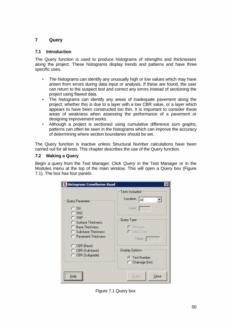
50

7 Query

7.1 Introduction

The Query function is used to produce histograms of strengths and thicknessesalong the project. These histograms display trends and patterns and have threespecific uses.

• The histograms can identify any unusually high or low values which may havearisen from errors during data input or analysis. If these are found, the usercan return to the suspect test and correct any errors instead of sectioning theproject using flawed data.

• The histograms can identify any areas of inadequate pavement along theproject, whether this is due to a layer with a low CBR value, or a layer whichappears to have been constructed too thin. It is important to consider theseareas of weakness when assessing the performance of a pavement ordesigning improvement works.

• Although a project is sectioned using cumulative difference sum graphs,patterns can often be seen in the histograms which can improve the accuracyof determining where section boundaries should be set.

The Query function is inactive unless Structural Number calculations have beencarried out for all tests. This chapter describes the use of the Query function.

7.2 Making a Query

Begin a query from the Test Manager. Click Query in the Test Manager or in theModules menu at the top of the main window. This will open a Query box (Figure7.1). The box has four panels.

Figure 7.1 Query box

51

7.2.1 Query Parameter

In the first panel, select one parameter from the following to display in the histogram.• SN• SNC• SNP

• Surface Thickness• Base Thickness• Sub-base Thickness• Pavement Thickness

• CBR (Base)• CBR (Sub-base)• CBR (Subgrade)

7.2.2 Tests Included

The location of a test is a mandatory field when site details are input. Since strengthsand thicknesses are likely to be different in, for example, the carriageway and theverge, it may not be informative to display these values on the same histogram.Therefore the tests from which the histogram will be formed should be selected fromthe following locations.

• All locations• Carriageway only (individual lanes may be selected)• Shoulder only• Verge only• Lay-by / other only

If this selection gives less than two tests for display, a warning message is shownand the query cannot be made.

7.2.3 Query Type

This panel is used to identify minimum or low values on the histograms. Theselection operates differently depending on which parameter is to be displayed andis described in 7.3.1 to 7.3.3 below.

7.2.4 Display Options

This panel is used to select whether the horizontal scale of the histogram will beChainage or Test number. In some projects more than one test may be carried out ata particular chainage, for instance in different lanes. If Chainage is selected, theresults from these tests will be shown at slightly different chainages so that the usercan see the results more clearly. The first test, by Test number, will be shown at therecorded chainage, the second will be shown at the recorded chainage plus onemetre, the third at the recorded chainage plus two metres and so on. Although Zoomcan be used to distinguish between the columns more clearly, they may still appearto be close together, particularly so for CBR histograms which contain moreinformation than Structural Number and thickness histograms. If this is the case, it isrecommended that a histogram is displayed by Test Number.

7.3 Displaying the Query results

After the four panels have been completed, click Query to display the requiredhistogram. The appearance of the histogram and the way in which low and minimumvalues are shown varies according to the parameter that is being displayed.

52

7.3.1 Structural Number

The Structural Number histogram (Figure 7.2) shows a series of columns, arrangedby chainage or test number, whose height is determined by SN, SNC or SNP. Thescales of the histogram are set automatically to best display the selected information.

The Query Type selection can be used if the user wants to check that, for example,the Structural Number is above a specified value at every test site. To do this, a LessThan value should be entered in the third panel of the Query box. A warning will begenerated if the entered value is outside a realistic range. This value is shown as ablue dotted horizontal line on the histogram. The columns of those tests whoseStructural Number is above the value are shown in yellow and the columns of thosetests whose Structural Number is below the value are shown in orange. A messageabove the histogram indicates at how many sites the Structural Number is below thevalue.

Figure 7.2 Structural Number histogram

Three items are available below the histogram.

Help Open this manual on the screen at the appropriate section.

Zoombox

Zoom allows the horizontal scale to be changed so that more detail is visible. If theZoom value is greater than 100, a horizontal scroll bar is provided. Zoom is useful ifmore than one test was carried out at a particular chainage and the columns aredisplayed by chainage.

Close Return to the Test Manager.

When the cursor is placed over a column, its value is displayed in a small box.

A histogram can be printed by clicking Print in the File menu at the top of the mainwindow. It can be exported as a bitmap by clicking Export in the File menu. BothPrint and Export are available by right-clicking on the histogram.

53

7.3.2 Layer or Pavement Thickness

The Thickness histogram (Figure 7.3) shows a series of columns, arranged bychainage or test number, whose height is determined by the thickness of thespecified layer. The scales of the histogram are set automatically to best display theselected information.

The Query Type selection can be used if the user wants to check that, for example, alayer or the entire pavement is thicker than a specified value at every test site. To dothis, a Less Than value should be entered in the third panel of the Query box. Awarning will be generated if the entered value is outside a realistic range. This valueis shown as a blue dotted horizontal line on the histogram. The columns of thosetests whose selected layer or pavement is thicker than the value are shown in yellowand the columns of those tests whose selected layer or pavement is thinner than thevalue are shown in orange. A message above the histogram indicates at how manysites the layer or pavement is thinner than the value.

Figure 7.3 Layer Thickness histogram

Three items are available below the histogram.

Help Open this manual on the screen at the appropriate section.

Zoombox

Zoom allows the horizontal scale to be changed so that more detail is visible. If theZoom value is greater than 100, a horizontal scroll bar is provided. Zoom is useful ifmore than one test was carried out at a particular chainage and the columns aredisplayed by chainage.

Close Return to the Test Manager.

When the cursor is placed over a column, its value is displayed in a small box.

A histogram can be printed by clicking Print in the File menu at the top of the mainwindow. It can be exported as a bitmap by clicking Export in the File menu. BothPrint and Export are available by right-clicking on the histogram.

54

7.3.3 CBR

The CBR histogram shows a series of columns, arranged by chainage or testnumber. The vertical scale is downwards. Each column is broken into pieces, eachpiece representing one Test layer within the base, sub-base or subgrade. The lengthof each piece represents the thickness of the Test layer that it represents. The CBRvalue of that Test layer, reduced if necessary to its limiting value of 150 or 50 asdescribed in 6.2.2, is placed at the mid-point of each piece. Thus if CBR (Base) hasbeen queried and three of the Test layers identified from the penetration data hadbeen defined as part of the Base, the column would have three pieces, each onewith its CBR value up to a maximum of 150. The scales of the histogram are setautomatically to best display the selected information.

The Query Type selection can be used in two ways.

Minimum (Figure 7.4)

The user wants to identify the Test layer within each test which has the lowest CBRvalue. To do this, Minimum should be selected in the third panel of the Query box.The piece of each column which represents the Test layer with the lowest CBR valueis shown in orange and all other pieces are shown in yellow. It should be noted thatdrilled layers identified during automatic layer analysis in the base and sub-base areassigned CBR values of 0 and are therefore likely to be shown in orange. These cannormally be identified as drilled layers from their CBR values. If two Test layers havethe same CBR value and that value is the minimum of the test, both pieces areshown in orange.

Figure 7.4 CBR histogram (Minimum)

55

Less Than (Figure 7.5)

The user wants to check that all Test layers within a pavement layer have a CBRvalue (reduced if necessary to its limiting value of 150 or 50) greater than a specifiedvalue at every test site. To do this, a Less Than value should be entered in the thirdpanel of the Query box. A warning will be generated if the entered value is outside arealistic range. The pieces of columns which represent Test layers whose CBR isabove the value are shown in yellow and the pieces of columns which represent Testlayers whose CBR is below the value are shown in orange. It should be noted thatdrilled layers identified during automatic layer analysis in the base and sub-base areassigned CBR values of 0 and are therefore likely to be shown in orange. These cannormally be identified as drilled layers from their CBR values.

Figure 7.5 CBR histogram (Less Than)

Three items are available below the histogram.

Help Open this manual on the screen at the appropriate section.

Zoombox

Zoom allows the horizontal scale to be changed so that more detail is visible. If theZoom value is greater than 100, a horizontal scroll bar is provided. Zoom is useful ifmore than one test was carried out at a particular chainage and the columns aredisplayed by chainage.

Close Return to the Test Manager.

A histogram can be printed by clicking Print in the File menu at the top of the mainwindow. It can be exported as a bitmap by clicking Export in the File menu. BothPrint and Export are available by right-clicking on the histogram.

56

8 Sectioning

8.1 Introduction

The Sectioning function is used to divide the project into sections which haveproperties that are both reasonably uniform and different from adjacent sections.

Sectioning is carried out using a cumulative difference sum graph and can be basedupon one or more of a number of parameters, including strengths and layerthicknesses. A cumulative difference sum graph is produced as follows. UK DCPaverages the selected parameter over the length of the project and then, for eachtest site, calculates the value of the average minus the parameter at that site. Thesevalues are then summed in turn starting at the first test to find the cumulativedifference sum at each site and the sum is plotted against chainage for the entireproject. This is a similar process to that described in 5.3 and Table 5.1. By the natureof the calculation, the cumulative difference sum graph will be zero at the final testsite. Cumulative difference sum graphs often take a sawtooth form, where a line ofconstant gradient represents a section where the parameter is uniform. Lines drawnat the peaks and troughs of the sawtooth represent the boundaries between uniformsections.

A project can be sectioned using more than one parameter. After sectioning hasbeen carried out using each selected parameter, a bar chart can be generated whichshows the sections derived from each parameter alongside each other. The user canthen compare the sections and define the Design Sections of the project. TheseDesign Sections can then be used to assess the performance of the pavement ordesign improvement works.

The Sectioning function is inactive unless Structural Number calculations have beencarried out for all tests. If the project has less than six tests, it is unlikely thatsectioning will produce useful results and therefore the function is also inactive in thiscase.

This chapter describes the use of the Sectioning function.

57

8.2 Sections box

Sectioning is carried out from the Sections box (Figure 8.1). Open this box byclicking Section in the Test Manager or in the Modules menu at the top of the mainwindow. The Sections box has two panels and several buttons.

Figure 8.1 Sections box (before sectioning)

8.2.1 Parameters

This panel contains a table and two buttons.

The table indicates which parameters have been used to section the project and thenumber of sections which were derived from each selected parameter. Sectioningcan be carried out using one or more of nine parameters.

• CBR (Base)• CBR (Sub-Base)• CBR (Subgrade)

• SN• SNP

• Surface Thickness• Base Thickness• Sub-base Thickness• Pavement Thickness

Two buttons are present in the Parameters panel.

DetermineSections

Section a project using a selected parameter. Its use is described in 8.3.1 below.

58

Summary Compare the sections derived from each selected parameter. It is not availableuntil sectioning has been carried out using at least one parameter. Its use isdescribed in 8.3.2 below.

8.2.2 Tests Included

The location of a test is a mandatory field when the Site details for that test areentered (4.2). Since strengths and thicknesses are likely to be different in, forexample, the carriageway and the verge, it may not be useful to section a projectusing results from all locations. Therefore the tests which will be used for sectioningshould be selected from the following locations.

• All locations• Carriageway only (individual lanes may be selected)• Shoulder only• Verge only• Lay-by / other only

If the selected location has less than six tests, it is unlikely that sectioning willproduce useful results and a warning message is generated stating that at least sixtests are required. Since all sectioning must be carried out using the same data,once sectioning has begun, it is not possible to change the choice of tests and thepanel is inactive.

8.2.3 Sections Buttons

There are six buttons at the bottom of the Sections box. Their use is described brieflybelow.Help Open this manual on the screen at the appropriate section.

Reset Allow the project to be reanalysed using tests in a differentlocation. This button is active after sectioning has begun or Edithas been clicked.

OK Accept and save the sectioning analysis and return to the TestManager. If Design Sections have been determined, it will beseen (Figure 8.9) that today’s date will be in the Sectioningcolumn for all tests.

Cancel Cancel the analysis which has just been carried out and return tothe Test Manager.

Edit Edit the sectioning analysis. Clicking this button allows the projectto be reanalysed using the same tests.

Close

Visible ifthe projecthas alreadybeensectionedand saved

Click this button to return to the Test Manager without making anyedits.

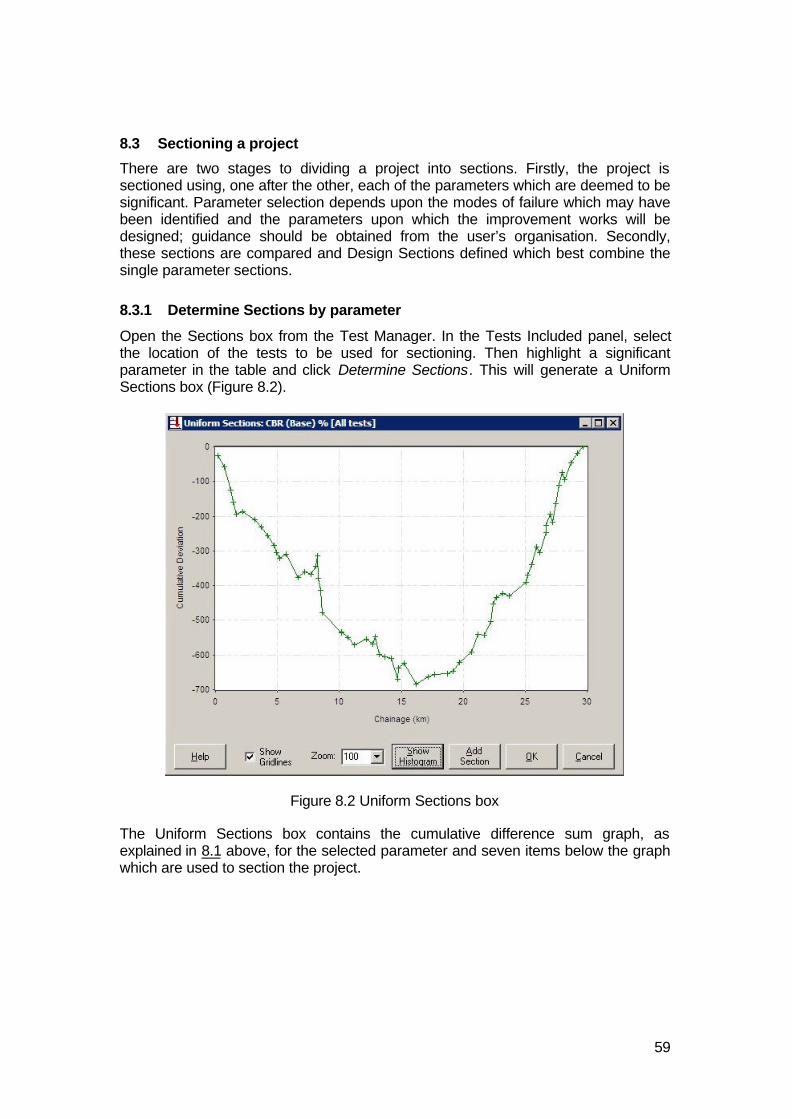
59

8.3 Sectioning a project

There are two stages to dividing a project into sections. Firstly, the project issectioned using, one after the other, each of the parameters which are deemed to besignificant. Parameter selection depends upon the modes of failure which may havebeen identified and the parameters upon which the improvement works will bedesigned; guidance should be obtained from the user’s organisation. Secondly,these sections are compared and Design Sections defined which best combine thesingle parameter sections.

8.3.1 Determine Sections by parameter

Open the Sections box from the Test Manager. In the Tests Included panel, selectthe location of the tests to be used for sectioning. Then highlight a significantparameter in the table and click Determine Sections. This will generate a UniformSections box (Figure 8.2).

Figure 8.2 Uniform Sections box

The Uniform Sections box contains the cumulative difference sum graph, asexplained in 8.1 above, for the selected parameter and seven items below the graphwhich are used to section the project.

60

Help Open this manual on the screen at the appropriate section.

ShowGridlines

A check box is provided to allow gridlines to be displayed or removed.

Zoom box Zoom allows the horizontal scale to be changed so that more detail is visible.If the Zoom value is greater than 100, a horizontal scroll bar is generated.

ShowHistogram

If the peaks and troughs of the cumulative difference sum graph are not clear,a histogram can help to identify section boundaries. Click this button todisplay a Histogram box (Figure 8.3) containing a histogram of the selectedparameter against chainage. The height of each column represents the valueof the parameter at that test point. In the case of CBR values, if the base, sub-base or subgrade comprise more than one Test layer, the CBR values ofthese Test layers (limited to 150 or 50 as described in 6.2.2) are combined togive an aggregate value. Within the base and sub-base, the Test layers areweighted according to their thicknesses but within the subgrade, the Testlayers are combined by the procedure referred to in 6.1.3 which derives anaggregate subgrade CBR in a manner which reflects engineering judgement.If a test was carried out at a chainage, but the parameter was zero, forexample if CBR (Sub-base) is selected, but no sub-base was identified, a boldline along the horizontal scale will be seen at that chainage. If no test wascarried out, only the fainter chainage scale will be visible. Within theHistogram box, Help opens this manual on the screen, Zoom allows moredetail to be seen and Close returns to the graph. When the cursor is placedover a column, its value is displayed in a small box.

Add Section Click the button and then click and hold the cursor on the white portion of thegraph. A vertical line will appear. Move the line until it is at a point where thegradient of the graph, and hence the parameter, makes a significant change.Since the cumulative difference sum is calculated from the lower chainageson the left towards the right, it is more accurate for a boundary to be placedmidway between a peak or trough and the point to its immediate right thanexactly at the peak or trough. Release the button to fix the section boundary.Add more boundaries as required. If a boundary is misplaced, it can be re-clicked and dragged or double-clicked and deleted. A graph with one sectionboundary added is shown in Figure 8.4. Since it is very rare for a cumulativedifference sum graph to be a perfect sawtooth, the user’s organisation shouldproduce guidance regarding how finely the project should be sectioned.

OK Save the sectioning and return to the Sections box. A number in the tablealongside the parameter will show into how many sections the project hasbeen divided for that parameter. Another significant parameter can then behighlighted for sectioning.

Cancel Cancel the sectioning and return to the Sections box.

61

Figure 8.3 Histogram of sectioning dataThis histogram displays the same data that was used to generate Figure 8.2.

Figure 8.4 Uniform Sections box (with one section boundary added)This graph is the same as shown in Figure 8.2.

62

After the project has been sectioned using all of the significant parameters, theSections box is as shown in Figure 8.5. In this case, design has focussed on thebase layer.

Figure 8.5 Sections box (after Sectioning)

8.3.2 Determine Design Sections for the project

The sectioning from all of the significant parameters can now be compared andDesign Sections defined. Click Summary in the Sections box to display a SectionSummary box (Figure 8.6). The Summary button will be enabled only after theuniform sectioning has been saved.

Figure 8.6 Section Summary box

63

The Section Summary box contains a series of parallel horizontal bars, one bar foreach selected parameter, as indicated on the left hand scale. Each bar extends fromthe chainage of the first included test to the chainage of the last included test. Oneach bar, every section boundary is marked with a bold line and the sections arecoloured alternately yellow and orange. A value in the centre of each section is theaverage value of the relevant parameter for all tests in the section. The user shouldcompare these bars in order to define the Design Sections of the project.

There are eight items below the horizontal bars.

Help Open this manual on the screen at the appropriate section.

Zoom box Zoom allows the horizontal scale to be changed so that more detailis visible. If the Zoom value is greater than 100, a horizontal scrollbar is provided.

DesignSectionProperties

This button is available after the first Design Section boundary hasbeen accepted. Click this button to generate a Design SectionProperties box (Figure 8.7) containing a table of Design Sectioninformation. For each Design Section, the table gives its start andend chainages, its length, the number of tests within it, and astatistical analysis of each of the nine parameters. Lower tenthpercentile values are not calculated for layer thicknesses, or for anyparameter if there are less than seven tests in a Design Section.The user should note that if a parameter in a section has a value ofzero, or if it is allocated a value of zero for an absent layer, thestatistical analysis will use this zero. Therefore averages and lowertenth percentiles may be lower than expected. To identify thesezeroes, and possibly delete or reanalyse a test, examine theminimum values for each parameter. Within the Design SectionProperties box, Help opens this manual on the screen and Closereturns to the Section Summary box.

AddDesignSection

This button is used to add a Design Section boundary to the seriesof horizontal bars. Click the button and then click and hold thecursor on the white portion of the graph. A vertical line will appear.Move the line until it is at a point which best represents a change inthe overall properties of the project. Release the button to fix theDesign Section boundary. Add more boundaries as required. If aboundary is misplaced, it can be re-clicked and dragged or double-clicked and deleted. It may be that all selected parameters havebeen sectioned at a similar point, in which case a boundary shouldbe placed in their midst, but if the sections are dispersed, guidancefrom the user’s organisation may be required to determine whichparameters may take precedence and where the Design Sectionboundary should be placed. Guidance should also be producedregarding how finely the project should be sectioned. A chart withone Design Section boundary added is shown in Figure 8.8.

OK Accept the Design Sections and enable the Design SectionProperties and Close buttons. Click Close to return to the Sectionsbox and then click Close in the Sections box to return to the TestManager. It will be seen (Figure 8.9) that today’s date will be in theSectioning column for all tests in the project.

Cancel Cancel the sectioning and return to the Sections box.

Edit Visible iftheprojecthasalreadybeensectionedand saved

Edit the sectioning analysis.

64

Close Click this button to return to the Sections box.

Figure 8.7 Design Section Properties box

Figure 8.8 Section Summary box (with one Design Section boundary added)

The addition of the Design Sections marks the end of the analysis of the penetrationdata. Reports which summarise the data, analysis and results can be produced.These are described in Chapter 9 below.

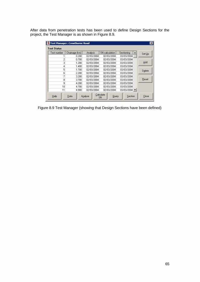
65

After data from penetration tests has been used to define Design Sections for theproject, the Test Manager is as shown in Figure 8.9.

Figure 8.9 Test Manager (showing that Design Sections have been defined)

66

9 Reporting

9.1 Introduction

The final function of UK DCP is the production of data, analysis and reports forprinting or export. All reports are selected from the Report menu at the top of themain window. They can be zoomed-in by double clicking with the left button andzoomed-out by double-clicking with the right button.

There are seven buttons at the bottom of each report.

Help Open this manual on the screen at the appropriate section.

Reset Returns to the top of the first page of the selected report.

Back If a report occupies more than one page, this button displays the previous page.

Next If a report occupies more than one page, this button displays the next page.

Print Generate a standard Print box. Select the printer and page and print as normal.

Export Generate an Export box (Figure 9.1). The report can be exported in one of fourformats: Windows Metafile (for use as a non-editable image), HTML (for use in awebsite), Clipboard (for temporary storage and pasting) and CSV (for use in aspreadsheet). Select the required format and click OK. Click Help to open thismanual on the screen and Cancel to return to the report. Reports which areincompatible with a spreadsheet cannot be exported in CSV format.

Close Close the report.

Figure 9.1 Export box

67

There are two types of reports: Test Reports and Project Reports.

9.2 Test Reports

Test Reports contain information from a single penetration test. Two Test Reportscan be produced.

9.2.1 Penetration Data

This report (Figure 9.2) can be produced after the penetration data has beenentered. Highlight the required test in the Test Manager and click Penetration Data inthe Report menu.

Figure 9.2 Penetration Data Report

68

The Report has the following six elements.• A header showing the UK DCP version number, the title of the report and the

project name.• A summary of test details, cone angle and upper layer information.• A table of original penetration data, including the penetration rate between

points.• Remarks if any were entered in the Site Details panel during data input.• Information about drilled layers and the use of an extension rod.• A footer showing when the report was produced and the page number of the

report. This report may occupy more than one page.

69

9.2.2 Layer Strength Analysis

This report (Figure 9.3) can be produced after the Structural Number calculationshave been carried out. Highlight the required test in the Test Manager and clickLayer Strength Analysis in the Report menu. As this report is not compatible with aspreadsheet, it cannot be exported in CSV format.

Figure 9.3 Layer Strength Analysis Report

70

The Report has the following nine elements.• A header showing the UK DCP version number, the title of the report and the

project name.• A summary of test details, cone angle and upper layer information.• A Layer Boundaries Chart.• A CBR Chart showing the CBR value of each test point and the CBR value of

each identified layer.• A Layer Properties table showing number, penetration rate, CBR (%) – not

reduced to its limiting value of 150 or 50, thickness, depth to underside oflayer, position (Base, Sub-base, etc) and strength coefficient for each Testlayer. This is similar to the table that was described in 6.2.2 above.

• A Pavement Strength table showing SN, SNC and SNP for each pavementlayer and for the entire pavement. This is the same table that is shown inFigure 6.5.

• The relationship which was used to convert the penetration rate to a CBRvalue, from those listed in Table 4.1.

• Space for the name of the producer of the report to be written.• A footer showing when the report was produced and that it occupies a single

page.

71

9.3 Project Reports

Project Reports contain information from the entire project. Three Project Reportscan be produced.

9.3.1 Section Summary

This report (Figure 9.4) can be produced after Design Sections have been defined.Click Section Summary in the Report menu. As this report is not compatible with aspreadsheet, it cannot be exported in CSV format.

Figure 9.4 Section Summary Report

The Report has the following five elements.• A header showing the UK DCP version number, the title of the report and the

project name.• A summary of the number of tests used for the sectioning and where they

were located.• A chart containing a series of parallel horizontal bars, one for each parameter

used when sectioning the project, and bold perpendicular lines to show whereDesign Section boundaries have been defined. The chart is the same as thechart in the Section Summary box in Figure 8.8.

• Space for the name of the producer of the report to be written.• A footer showing when the report was produced and that it occupies a single

page.

72

9.3.2 Design Section Properties

This report (Figure 9.5) can be produced after Design Sections have been defined.Click Design Section Properties in the Report menu.

Figure 9.5 Design Section Properties Report

The Report has the following four elements.• A header showing the UK DCP version number, the title of the report and the

project name.• A summary of the number of tests used for the sectioning and where they

were located.• A table showing, for each Design Section, the start and end chainages, its

length, the number of test within it, and a statistical analysis of nine strengthand thickness parameters. This table is similar to that in the Design SectionProperties box in Figure 8.7.

• A footer showing when the report was produced and the page number of thereport. This report may occupy more than one page.

73

9.3.3 Project Summary

This report (Figure 9.6) can be produced after Design Sections have been defined.Click Project Summary in the Report menu.

Figure 9.6 Project Summary Report

The Report has the following three elements.• A header showing the UK DCP version number, the title of the report and the

project name.• A table summarising the test details, Upper layers and Test layers and

calculated pavement strengths of each test in the project.• A footer showing when the report was produced and the page number of the

report. This report may occupy more than one page.

74

10 References

1. Jones C R and J Rolt (1991). Operating instructions for the TRL dynamic conepenetrometer (2nd edition). Information Note. Crowthorne: Transport ResearchLaboratory

2. User Manual, WinDCP 5.0 software, 2001. CSIR, South Africa

3. Kleyn K G & P F Savage (1982). The application of the pavement DCP todetermine the bearing properties and performance of Road Pavements. InternationalSymposium on Bearing Capacity of Roads and Airfields. Trondheim, Norway

4. Transport and Road Research Laboratory (1990). A users manual for a programto analyse dynamic cone penetrometer data. Overseas Road Note 8. TransportResearch Laboratory, Crowthorne

5. MacNeil D J and D P Steele, (2002). Granular and bituminous planings mixturesfor capping. TRL Report TRL523. TRL Limited, Crowthorne, UK

6. Smith R B and Pratt D N (1983). A field study of in situ California bearing ratioand dynamic cone penetrometer testing for road subgrade investigations. AustralianRoad Research 13(4) December 1983 pp285-294. (Australian Road ResearchBoard)

7. American Association of State Highway and Transportation Officials (AASHTO)(1993). AASHTO guide for design of pavement structures. Washington DC: AASHTO

8. Hodges J W, J Rolt and T.E Jones (1975). The Kenya road transport cost study:research on road deterioration. TRRL Research Report LR 673.Transport and RoadResearch Laboratory, Crowthorne, UK

9. Rolt J and C C Parkman (2000). Characterisation of Pavement Strength in HDMIII and changes adopted for HDM-4. 10th International Conference of the RoadEngineering Association of Asia and Australia

10. Morosiuk G, M J Riley, W D O Paterson, J B Odoki, J P Covarrubibus (2000).Modelling road deterioration and works effects. Volume 6 of the HDM 4 series ofpublications. PIARC ISOHDM