User Manual Module 3 Liner selection

Civil Engineering

User Manual Module 3 – Liner selection

AUTHORS: Rukshan Azoor, Benjamin Shannon,

Guoyang Fu, Ravin Deo, Jayantha Kodikara.

28 / 06 / 2021

UM M3 – Liner selection| ii

QUALITY INFORMATION

Document: User Manual, Module 3 – Liner selection

Edition date: 28-06-2021

Edition number: 1.1

Prepared by: Rukshan Azoor

Reviewed by: Benjamin Shannon, Guoyang Fu

Revision history

Revision Revision date Details Revised by

1 28-06-2021 Updated nomenclature, minor revisions Rukshan Azoor

UM M3 – Liner selection| iii

CONTENTS

Contents ............................................................................................................................................................ iii

Acknowledgements ............................................................................................................................................ iv

Introduction ........................................................................................................................................................ 1

1 Calculation process ............................................................................................................................................................1

1.1 Step I-Failure history...................................................................................................................................................2

1.2 Step II - Deterioration..................................................................................................................................................4

1.3 Step III - Leak rates ....................................................................................................................................................7

2 Summary of inputs, outputs and workflow ..........................................................................................................................8

3 Zone level analysis; multiple pipe calculations .................................................................................................................10

Nomenclature .................................................................................................................................................. 12

Disclaimer ........................................................................................................................................................ 14

References ...................................................................................................................................................... 14

A. Annex – Utility data pre-processing .......................................................................................................................... 15

UM M3 – Liner selection | iv

ACKNOWLEDGEMENTS

The Australian Government, through the Cooperative Research Centre, provided funding for the Smart Linings for Pipe and Infrastructure Project that produced this report. The CRC Program supports industry-led collaborations between industry, researchers and the community.

The project was led by the Water Services Association of Australia (WSAA) and included the following project partners, all of whom contributed expertise, labour, funding, products or trial sites to assist in the delivery of this project.

Abergeldie Watertech

BASF Australia

Bisley & Company

Calucem GmbH

Central Highlands Water

City West Water Corporation

Coliban Region Water Corporation

Downer

GeoTree Solutions

Hunter Water Corporation

Hychem International

Icon Water

Insituform Pacific

Interflow

Melbourne Water Corporation

Metropolitan Restorations

Monash University

Nu Flow Technologies

Parchem Construction Supplies

Sanexen Environmental Services

SA Water Corporation

South East Water Corporation

Sydney Water Corporation

The Australasian Society for Trenchless Technology (ASTT)

The Water Research Foundation

UK Water Industry Research Ltd (UKWIR)

Unitywater

University of Sydney

University of Technology Sydney

Urban Utilities

Ventia

Water Corporation

Wilsons Pipe Solutions

Yarra Valley Water

UM M3 – Liner selection | 1

INTRODUCTION

This document outlines the methods and processes used in the liner selection module (Figure 1), and provides guidelines for its use. Descriptions for the text highlighted in bold are provided in the nomenclature section.

Figure 1. Liner selection module icon in the user interface

The primary function of the liner selection module is to provide an initial estimate of a suitable lining type/method or any other renewal recommendation based on the available information about the pipeline/network. The calculations can be performed on an individual pipe segment or on a collection or a group of pipelines herein termed a zone. The option to select the analysis approach is provided at the start of the module (Figure 2).

Figure 2. Pipe level analysis and Zone level analysis icons

In pipe level analysis, the user is guided through a workflow to arrive at the initial liner decision based on information for one pipe segment. In zone level analysis, a batch calculation is performed on a pipe list that is input by the user. In both approaches, the available information is used to establish the level of deterioration of the pipe and a respective condition grade. Recommendations are based directly on the condition grade.

1 CALCULATION PROCESS

The calculation process is organised into a three-step simple workflow to determine the condition grade of a pipeline before recommending a suitable liner. The condition grade is evaluated using three methods, which can be used separately or in combination, depending on the level of available information. The three methods are, pipe failure history, deterioration and leak rates. The methods


are implemented in the above given order within the web application to arrive at the final recommendation. These methods are explained below.

1.1 Step I-Failure history

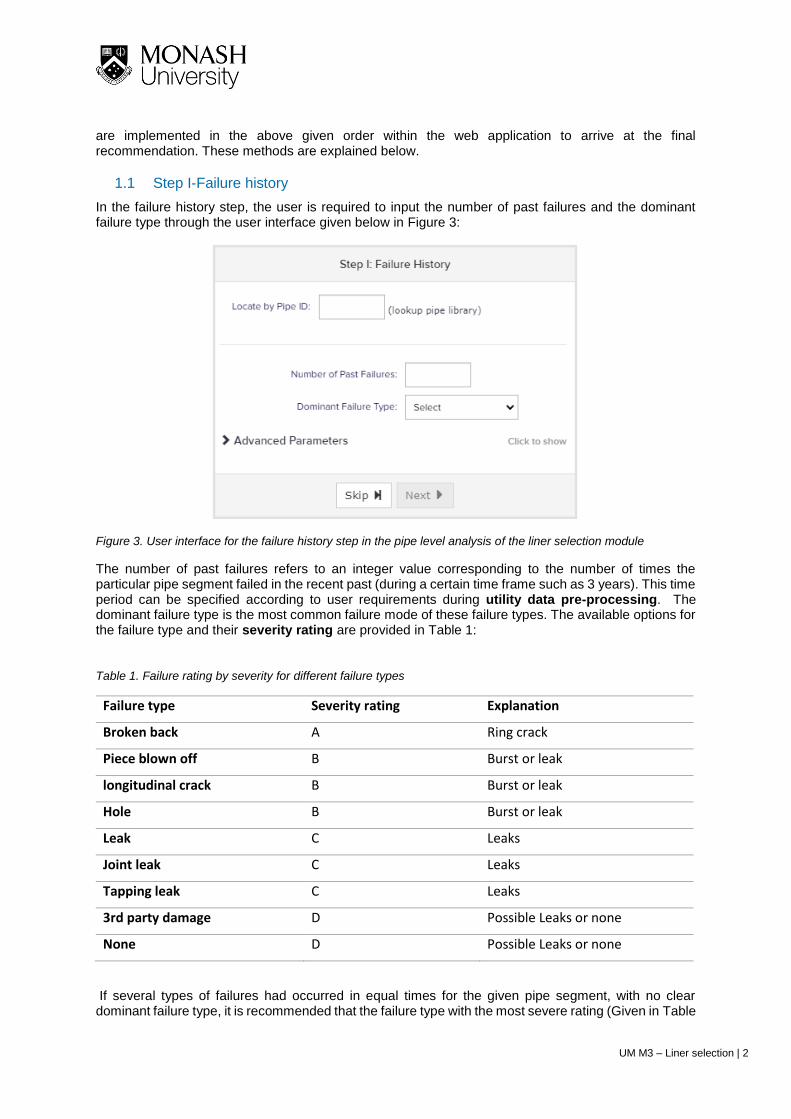
In the failure history step, the user is required to input the number of past failures and the dominant failure type through the user interface given below in Figure 3:

Figure 3. User interface for the failure history step in the pipe level analysis of the liner selection module

The number of past failures refers to an integer value corresponding to the number of times the particular pipe segment failed in the recent past (during a certain time frame such as 3 years). This time period can be specified according to user requirements during utility data pre-processing. The dominant failure type is the most common failure mode of these failure types. The available options for the failure type and their severity rating are provided in Table 1:

Table 1. Failure rating by severity for different failure types

Failure type Severity rating Explanation

Broken back A Ring crack

Piece blown off B Burst or leak

longitudinal crack B Burst or leak

Hole B Burst or leak

Leak C Leaks

Joint leak C Leaks

Tapping leak C Leaks

3rd party damage D Possible Leaks or none

None D Possible Leaks or none

If several types of failures had occurred in equal times for the given pipe segment, with no clear dominant failure type, it is recommended that the failure type with the most severe rating (Given in Table


1; with a rating A being the most severe and D being the least severe) be selected as the dominant failure type. Once these inputs are set, the calculation can proceed to the next step. Alternatively, the relevant input parameters can also be extracted from the pipe library by pipe ID look up.

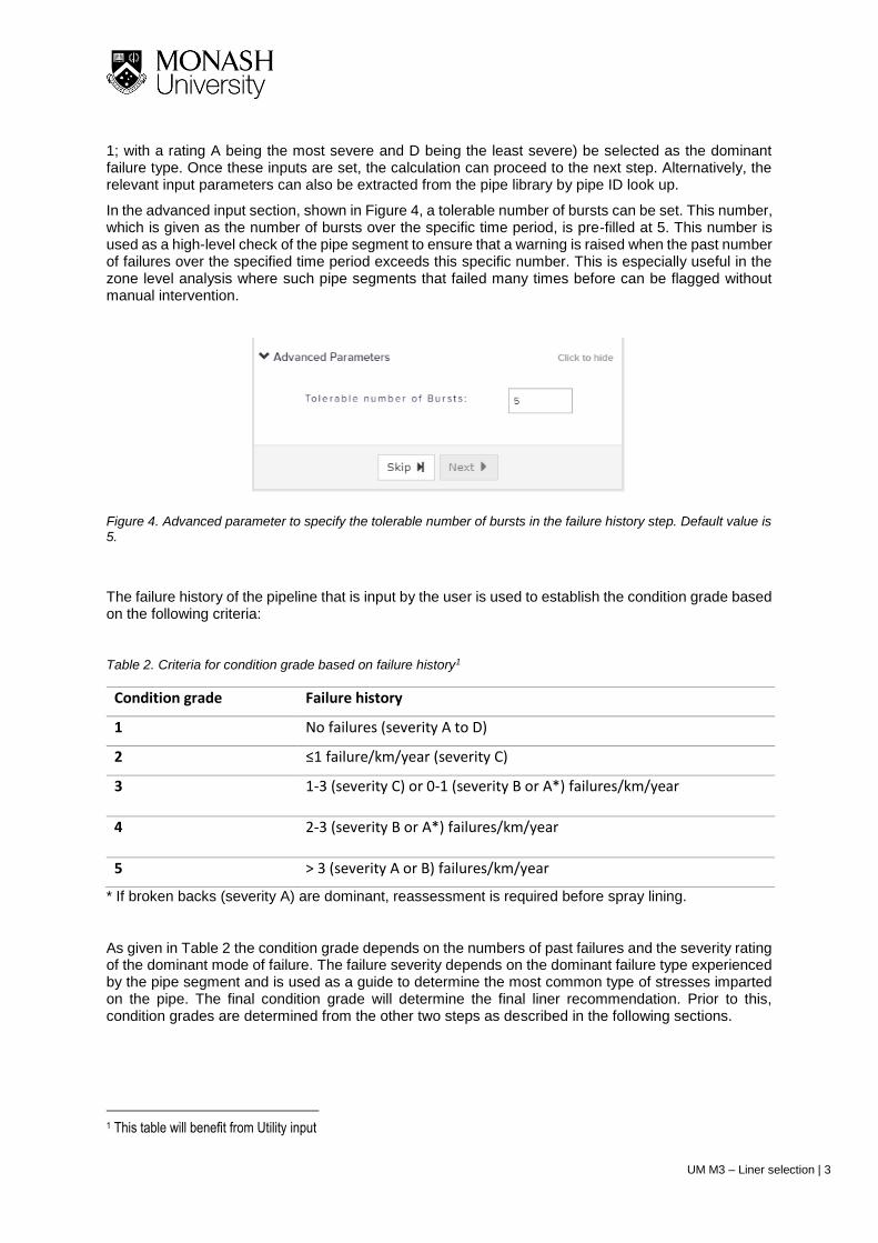
In the advanced input section, shown in Figure 4, a tolerable number of bursts can be set. This number, which is given as the number of bursts over the specific time period, is pre-filled at 5. This number is used as a high-level check of the pipe segment to ensure that a warning is raised when the past number of failures over the specified time period exceeds this specific number. This is especially useful in the zone level analysis where such pipe segments that failed many times before can be flagged without manual intervention.

Figure 4. Advanced parameter to specify the tolerable number of bursts in the failure history step. Default value is 5.

The failure history of the pipeline that is input by the user is used to establish the condition grade based on the following criteria:

Table 2. Criteria for condition grade based on failure history1

Condition grade Failure history

1 No failures (severity A to D)

2 ≤1 failure/km/year (severity C)

3 1-3 (severity C) or 0-1 (severity B or A*) failures/km/year

4 2-3 (severity B or A*) failures/km/year

5 > 3 (severity A or B) failures/km/year

* If broken backs (severity A) are dominant, reassessment is required before spray lining.

As given in Table 2 the condition grade depends on the numbers of past failures and the severity rating of the dominant mode of failure. The failure severity depends on the dominant failure type experienced by the pipe segment and is used as a guide to determine the most common type of stresses imparted on the pipe. The final condition grade will determine the final liner recommendation. Prior to this, condition grades are determined from the other two steps as described in the following sections.

1 This table will benefit from Utility input


1.2 Step II - Deterioration

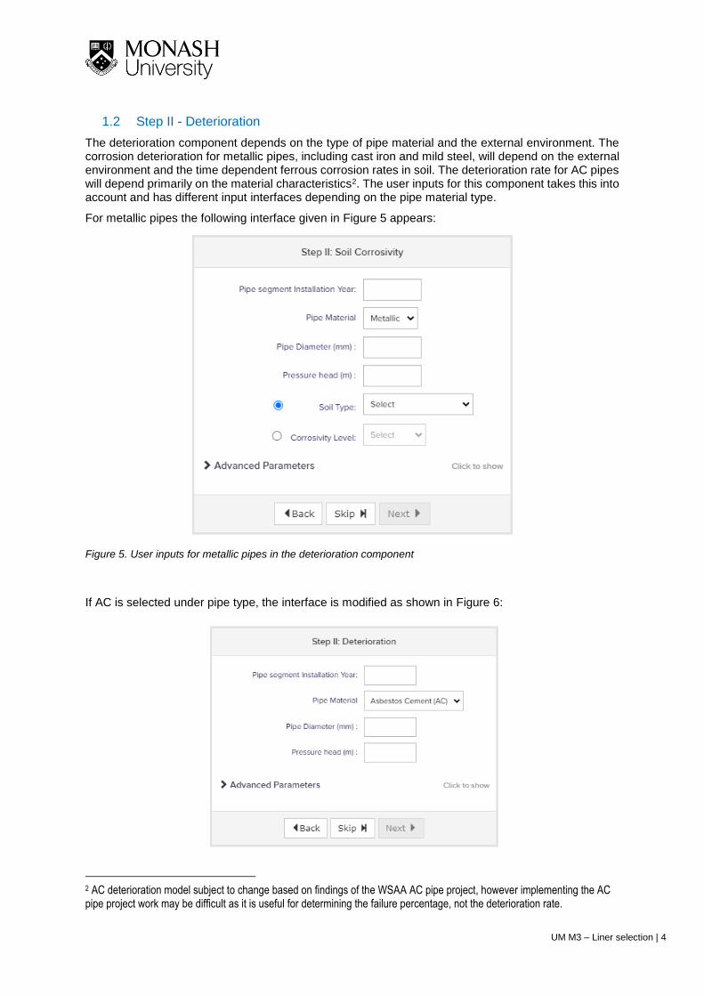
The deterioration component depends on the type of pipe material and the external environment. The corrosion deterioration for metallic pipes, including cast iron and mild steel, will depend on the external environment and the time dependent ferrous corrosion rates in soil. The deterioration rate for AC pipes will depend primarily on the material characteristics2. The user inputs for this component takes this into account and has different input interfaces depending on the pipe material type.

For metallic pipes the following interface given in Figure 5 appears:

Figure 5. User inputs for metallic pipes in the deterioration component

If AC is selected under pipe type, the interface is modified as shown in Figure 6:

2 AC deterioration model subject to change based on findings of the WSAA AC pipe project, however implementing the AC pipe project work may be difficult as it is useful for determining the failure percentage, not the deterioration rate.


Figure 6. Input fields for AC pipes in the deterioration step

The information on installation year, pipe diameter and pressure head are used to calculate the pipe wall thickness and material properties for both types of pipe based on cohort analysis. (See the document: TM M2 Part 1 – Pipe cohorts 3 [2] for a description of cohort analysis methods used for this purpose)

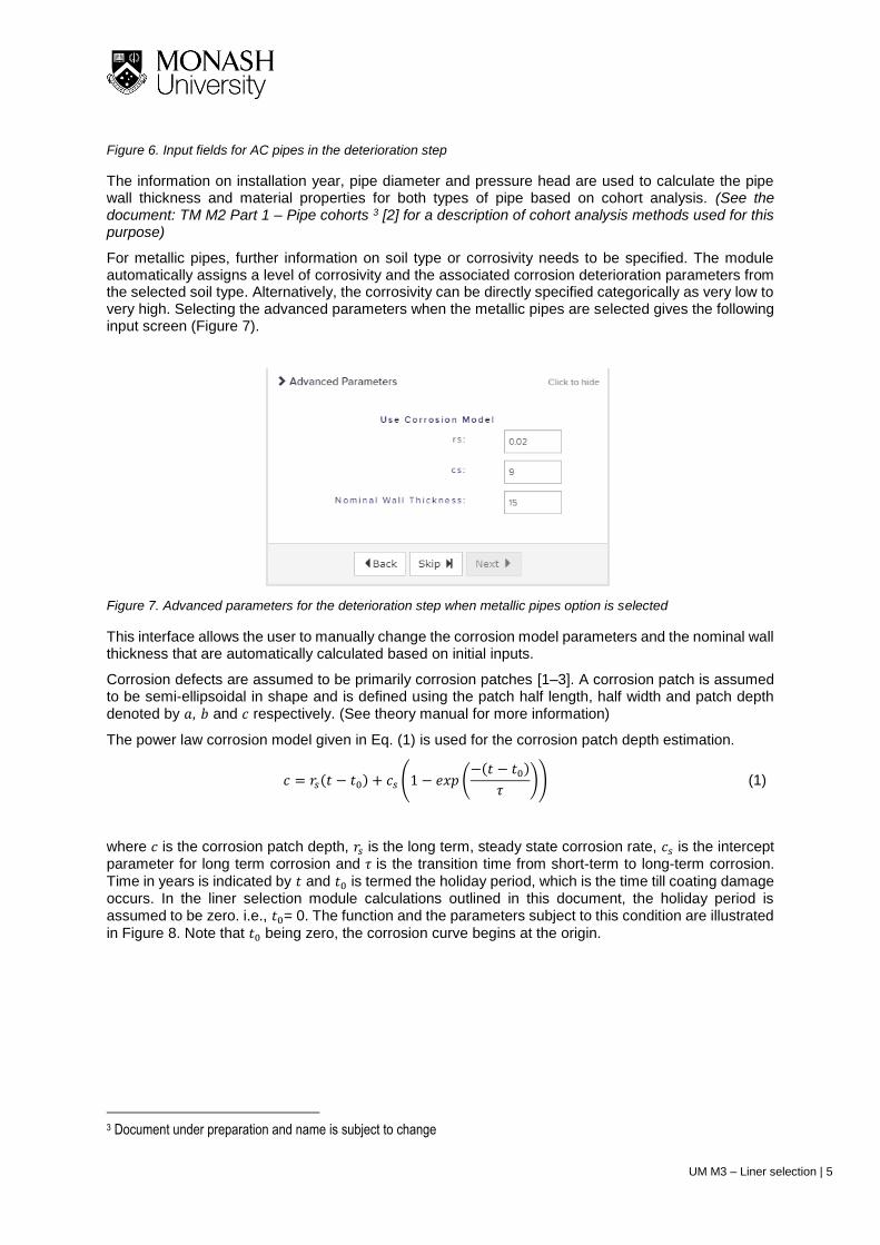
For metallic pipes, further information on soil type or corrosivity needs to be specified. The module automatically assigns a level of corrosivity and the associated corrosion deterioration parameters from the selected soil type. Alternatively, the corrosivity can be directly specified categorically as very low to very high. Selecting the advanced parameters when the metallic pipes are selected gives the following input screen (Figure 7).

Figure 7. Advanced parameters for the deterioration step when metallic pipes option is selected

This interface allows the user to manually change the corrosion model parameters and the nominal wall thickness that are automatically calculated based on initial inputs.

Corrosion defects are assumed to be primarily corrosion patches [1–3]. A corrosion patch is assumed to be semi-ellipsoidal in shape and is defined using the patch half length, half width and patch depth denoted by 𝑎, 𝑏 and 𝑐 respectively. (See theory manual for more information)

The power law corrosion model given in Eq. (1) is used for the corrosion patch depth estimation.

𝑐 = 𝑟𝑠(𝑡 − 𝑡0) + 𝑐𝑠 (1 − 𝑒𝑥𝑝 (−(𝑡 − 𝑡0)

𝜏)) (1)

where 𝑐 is the corrosion patch depth, 𝑟𝑠 is the long term, steady state corrosion rate, 𝑐𝑠 is the intercept parameter for long term corrosion and 𝜏 is the transition time from short-term to long-term corrosion.

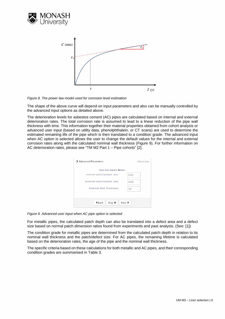
Time in years is indicated by 𝑡 and 𝑡0 is termed the holiday period, which is the time till coating damage occurs. In the liner selection module calculations outlined in this document, the holiday period is assumed to be zero. i.e., 𝑡0= 0. The function and the parameters subject to this condition are illustrated

in Figure 8. Note that 𝑡0 being zero, the corrosion curve begins at the origin.

3 Document under preparation and name is subject to change


Figure 8. The power law model used for corrosion level estimation

The shape of the above curve will depend on input parameters and also can be manually controlled by the advanced input options as detailed above.

The deterioration levels for asbestos cement (AC) pipes are calculated based on internal and external deterioration rates. The total corrosion rate is assumed to lead to a linear reduction of the pipe wall thickness with time. This information together their material properties obtained from cohort analysis or advanced user input (based on utility data, phenolphthalein, or CT scans) are used to determine the estimated remaining life of the pipe which is then translated to a condition grade. The advanced input when AC option is selected allows the user to change the default values for the internal and external corrosion rates along with the calculated nominal wall thickness (Figure 9). For further information on AC deterioration rates, please see “TM M2 Part 1 – Pipe cohorts” [2].

Figure 9. Advanced user input when AC pipe option is selected

For metallic pipes, the calculated patch depth can also be translated into a defect area and a defect size based on normal patch dimension ratios found from experiments and past analysis. (See: [1])

The condition grade for metallic pipes are determined from the calculated patch depth in relation to its nominal wall thickness and the patch/defect size. For AC pipes, the remaining lifetime is calculated based on the deterioration rates, the age of the pipe and the nominal wall thickness.

The specific criteria based on these calculations for both metallic and AC pipes, and their corresponding condition grades are summarised in Table 3.


Table 3. Condition grade calculation criteria used in the deterioration step for metallic and AC pipes

Condition grade Cast iron

Deterioration

Asbestos cement

Remaining life in years

1 Patch depth <50% wall thickness 50 or more

2 Patch depth between 50-80% wall thickness

20

3 Patch depth >80% wall thickness

Defect size <1000 mm2 if present

10

4 Defect size 1000-2000 mm2 5

5 Defect size >2000 mm2 0

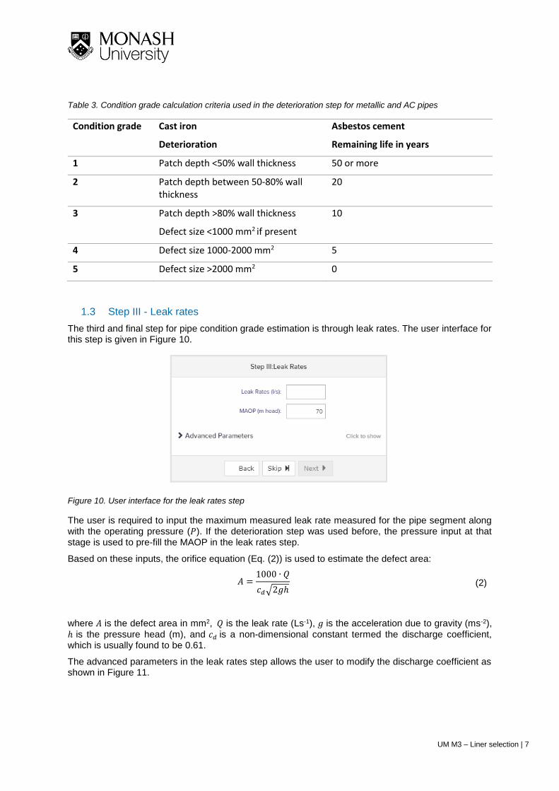
1.3 Step III - Leak rates

The third and final step for pipe condition grade estimation is through leak rates. The user interface for this step is given in Figure 10.

Figure 10. User interface for the leak rates step

The user is required to input the maximum measured leak rate measured for the pipe segment along with the operating pressure (𝑃). If the deterioration step was used before, the pressure input at that stage is used to pre-fill the MAOP in the leak rates step.

Based on these inputs, the orifice equation (Eq. (2)) is used to estimate the defect area:

𝐴 =1000 ∙ 𝑄

𝑐𝑑√2𝑔ℎ (2)

where 𝐴 is the defect area in mm2, 𝑄 is the leak rate (Ls-1), 𝑔 is the acceleration due to gravity (ms-2),

ℎ is the pressure head (m), and 𝑐𝑑 is a non-dimensional constant termed the discharge coefficient, which is usually found to be 0.61.

The advanced parameters in the leak rates step allows the user to modify the discharge coefficient as shown in Figure 11.


Figure 11. Advanced parameters for the leak rates step

The calculated defect areas are used to determine a condition grade similar to previous steps.

However, as the presence of a leak indicates that the host pipe is already compromised, and that the pipe cannot be in good condition, only the worst grades of 4 or 5 are assigned based on leak rates. Thus, the area calculated from the orifice equation is compared against a critical defect area of 1000 mm2 to assign the condition grade as given below in Table 4.

Table 4. Condition grade calculation from leak rates

Condition grade Defect area calculated from Leak rate

4 < 1000 mm2

5 > 1000 mm2

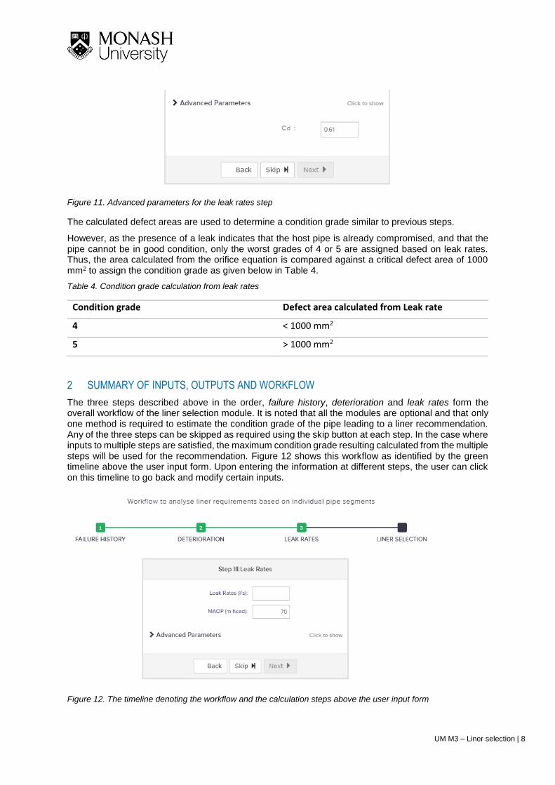
2 SUMMARY OF INPUTS, OUTPUTS AND WORKFLOW

The three steps described above in the order, failure history, deterioration and leak rates form the overall workflow of the liner selection module. It is noted that all the modules are optional and that only one method is required to estimate the condition grade of the pipe leading to a liner recommendation. Any of the three steps can be skipped as required using the skip button at each step. In the case where inputs to multiple steps are satisfied, the maximum condition grade resulting calculated from the multiple steps will be used for the recommendation. Figure 12 shows this workflow as identified by the green timeline above the user input form. Upon entering the information at different steps, the user can click on this timeline to go back and modify certain inputs.

Figure 12. The timeline denoting the workflow and the calculation steps above the user input form


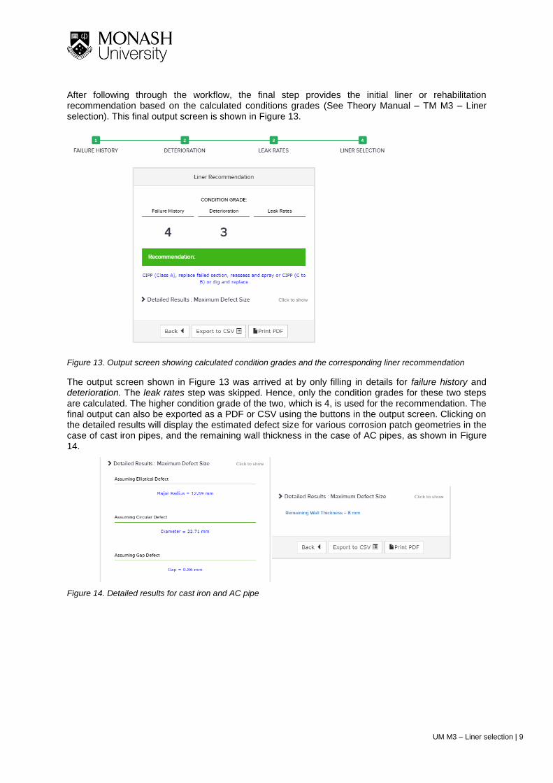
After following through the workflow, the final step provides the initial liner or rehabilitation recommendation based on the calculated conditions grades (See Theory Manual – TM M3 – Liner selection). This final output screen is shown in Figure 13.

Figure 13. Output screen showing calculated condition grades and the corresponding liner recommendation

The output screen shown in Figure 13 was arrived at by only filling in details for failure history and deterioration. The leak rates step was skipped. Hence, only the condition grades for these two steps are calculated. The higher condition grade of the two, which is 4, is used for the recommendation. The final output can also be exported as a PDF or CSV using the buttons in the output screen. Clicking on the detailed results will display the estimated defect size for various corrosion patch geometries in the case of cast iron pipes, and the remaining wall thickness in the case of AC pipes, as shown in Figure 14.

Figure 14. Detailed results for cast iron and AC pipe


3 ZONE LEVEL ANALYSIS; MULTIPLE PIPE CALCULATIONS

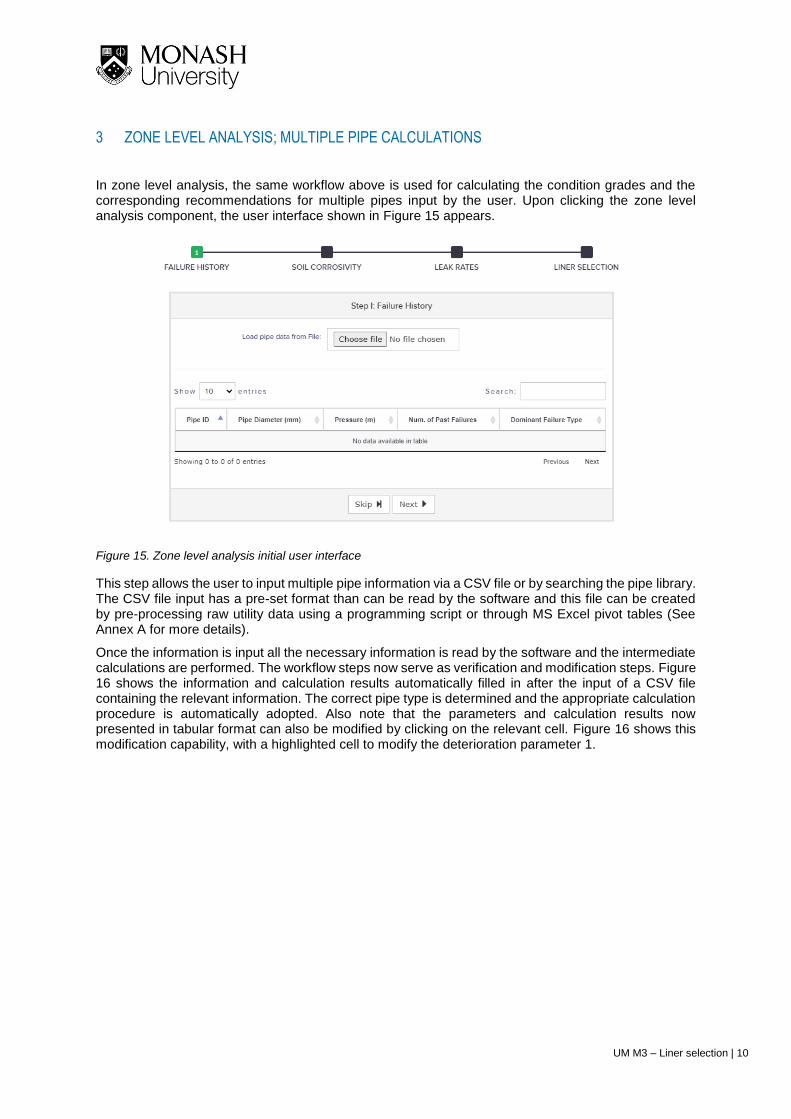
In zone level analysis, the same workflow above is used for calculating the condition grades and the corresponding recommendations for multiple pipes input by the user. Upon clicking the zone level analysis component, the user interface shown in Figure 15 appears.

Figure 15. Zone level analysis initial user interface

This step allows the user to input multiple pipe information via a CSV file or by searching the pipe library. The CSV file input has a pre-set format than can be read by the software and this file can be created by pre-processing raw utility data using a programming script or through MS Excel pivot tables (See Annex A for more details).

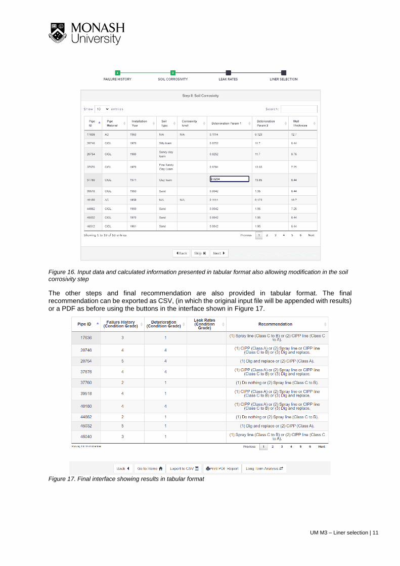
Once the information is input all the necessary information is read by the software and the intermediate calculations are performed. The workflow steps now serve as verification and modification steps. Figure 16 shows the information and calculation results automatically filled in after the input of a CSV file containing the relevant information. The correct pipe type is determined and the appropriate calculation procedure is automatically adopted. Also note that the parameters and calculation results now presented in tabular format can also be modified by clicking on the relevant cell. Figure 16 shows this modification capability, with a highlighted cell to modify the deterioration parameter 1.


Figure 16. Input data and calculated information presented in tabular format also allowing modification in the soil corrosivity step

The other steps and final recommendation are also provided in tabular format. The final recommendation can be exported as CSV, (in which the original input file will be appended with results) or a PDF as before using the buttons in the interface shown in Figure 17.

Figure 17. Final interface showing results in tabular format


NOMENCLATURE

Condition grade – A number from 1 to 5 indicating the severity of the deterioration of the pipeline. 5 being the most severely deteriorated and 1 being a pipe in pristine condition.

Step I pipe failure history – The calculation step where the past number of failures over a given time period and the domain failure type experienced during that period are used to estimate a condition grade for a pipe segment

Step II deterioration – The calculation step where the pipe material, age and soil conditions are used to estimate the level of deterioration based on available deterioration models, to finally estimate a condition grade for the pipe segment

Step III leak rates – The calculation step where measured leak rates are used to estimate the defect size based on the orifice equation to finally estimate the condition grade of the pipe segment

Severity rating – A rating assigned to a failure type ranging from A – D with A being the most severe and D the least severe.

Utility data pre-processing (see Annex A for more details) – A method to format raw data from utilities to the input format of the pipe evaluation platform. Processing can be done through programming scripts developed by Monash University or using the pivot table functionality in MS Excel.

2𝑎 Patch length (mm)

2𝑏 Patch width (mm)

𝑐 Patch depth (mm)

𝑘1 Patch factor

𝑘2 Aspect ratio

𝑟𝑠 Minimum corrosion rate (long-term) of metallic pipes (mm/y)

𝑐𝑠 Intercept parameter for long-term corrosion of metallic pipes (mm)

𝜏 Transition period between short-term and long-term corrosion (y)

𝑃 Operating pressure (MPa)

ℎ Pressure head (m)

𝑟𝑠𝑣 Radial corrosion rate for metallic pipes (mm/y)

𝑟𝑠ℎ Lateral extension rate for metallic pipes (mm/y)

𝑇𝑓 AC pipe remaining wall thickness at failure (mm)

𝑦𝑓 Predicted year for failure of an AC pipe (mm)

𝑐𝐴𝐶𝑖 Internal deterioration rate for AC pipes (mm/y)

𝑐𝐴𝐶𝑒 External deterioration rate for AC pipes (mm/y)

𝑄 Leak rate (L/s)

𝑐𝑑 Discharge coefficient

𝐴 Area of flow (mm2)

𝑔 Acceleration due to gravity (m/s2)


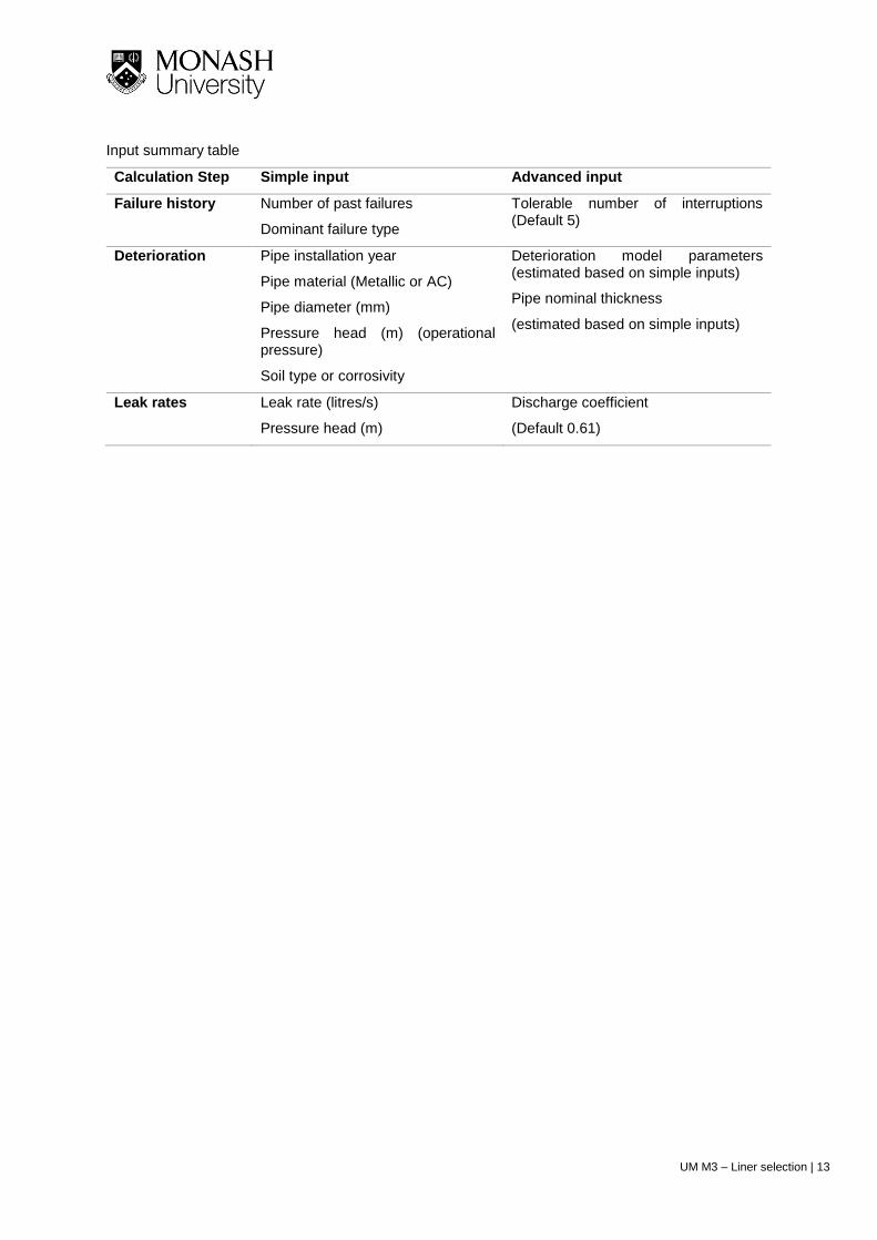
Input summary table

Calculation Step Simple input Advanced input

Failure history Number of past failures

Dominant failure type

Tolerable number of interruptions (Default 5)

Deterioration Pipe installation year

Pipe material (Metallic or AC)

Pipe diameter (mm)

Pressure head (m) (operational pressure)

Soil type or corrosivity

Deterioration model parameters (estimated based on simple inputs)

Pipe nominal thickness

(estimated based on simple inputs)

Leak rates Leak rate (litres/s)

Pressure head (m)

Discharge coefficient

(Default 0.61)


DISCLAIMER

1. Use of the information and data contained within the Liner Selection Module is at your sole risk.

2. If you rely on the information in the Liner Selection Module, then you are responsible for ensuring by independent verification of its accuracy, currency, or completeness.

3. The information and data in the Liner Selection Module is subject to change without notice.

4. The Liner Selection Module developers may revise this disclaimer at any time by updating the Pipe Liner Selection Module.

5. Monash University and the developers accept no liability however arising for any loss resulting from the use of the Liner Selection Module and any information and data.

REFERENCES

[1] Deo, R. N., Rathnayaka, S., Zhang, C., Fu, G. Y., Shannon, B., Wong, L. & Kodikara, J. K. Characterization of corrosion morphologies from deteriorated underground cast iron water pipes. Materials and Corrosion, 70(10):1837-1851

[2] Shannon, B., Fu, G., Azoor, R., Deo, R. and Kodikara, J. (2021). TM M2 Part 1 – Pipe cohorts

[3] Azoor, R., Shannon, B., Fu, G., Deo, R. and Kodikara, J. (2021). TM M3 – Liner selection


A. Annex – Utility data pre-processing

For the efficient use of the zone level analysis component in the liner selection module, it may be required to directly input utility data into the platform. Prior to using utility data, the data needs to be formatted to match the input format of the zone level analysis component. Methods and programming scripts have been developed for this purpose, with plans to include them as a separate component in the platform. This section outlines the steps in using these methods.

Method 1: Using MS Excel pivot tables

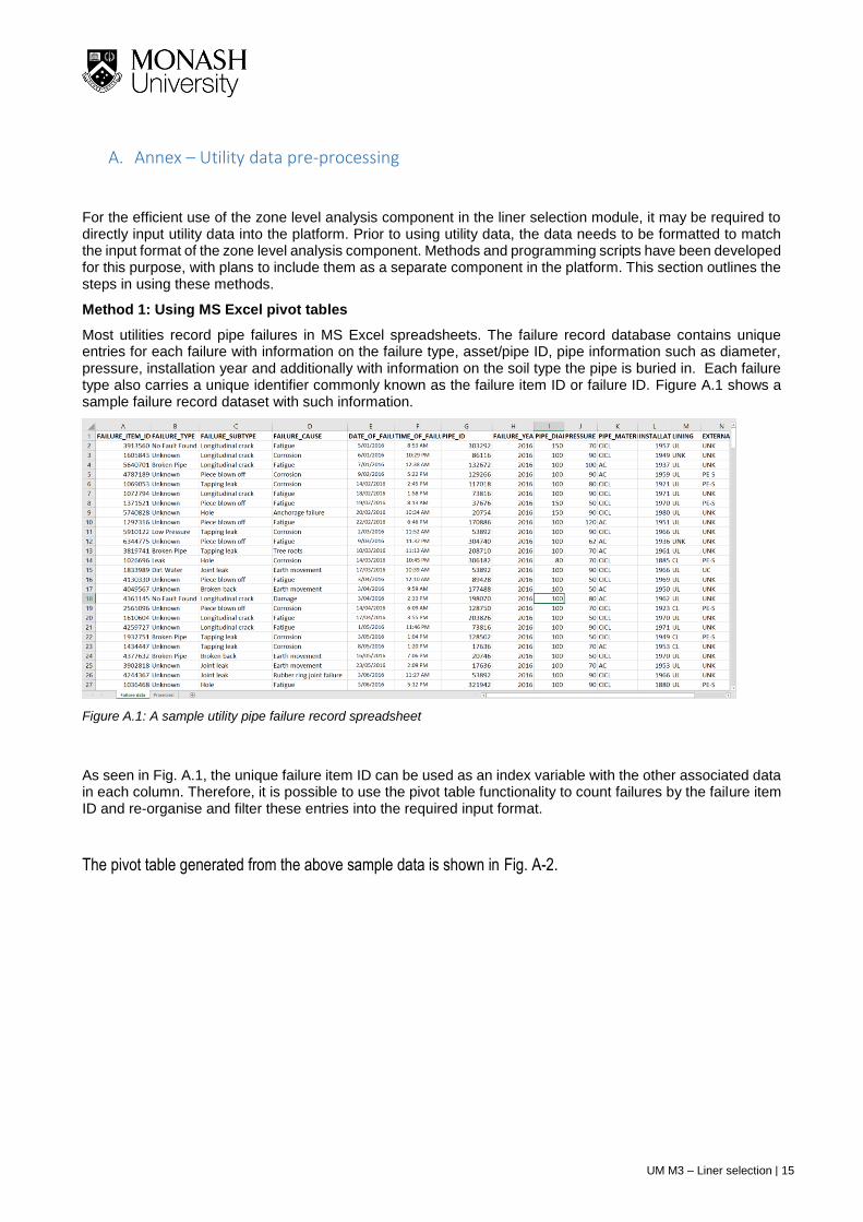
Most utilities record pipe failures in MS Excel spreadsheets. The failure record database contains unique entries for each failure with information on the failure type, asset/pipe ID, pipe information such as diameter, pressure, installation year and additionally with information on the soil type the pipe is buried in. Each failure type also carries a unique identifier commonly known as the failure item ID or failure ID. Figure A.1 shows a sample failure record dataset with such information.

Figure A.1: A sample utility pipe failure record spreadsheet

As seen in Fig. A.1, the unique failure item ID can be used as an index variable with the other associated data in each column. Therefore, it is possible to use the pivot table functionality to count failures by the failure item ID and re-organise and filter these entries into the required input format.

The pivot table generated from the above sample data is shown in Fig. A-2.


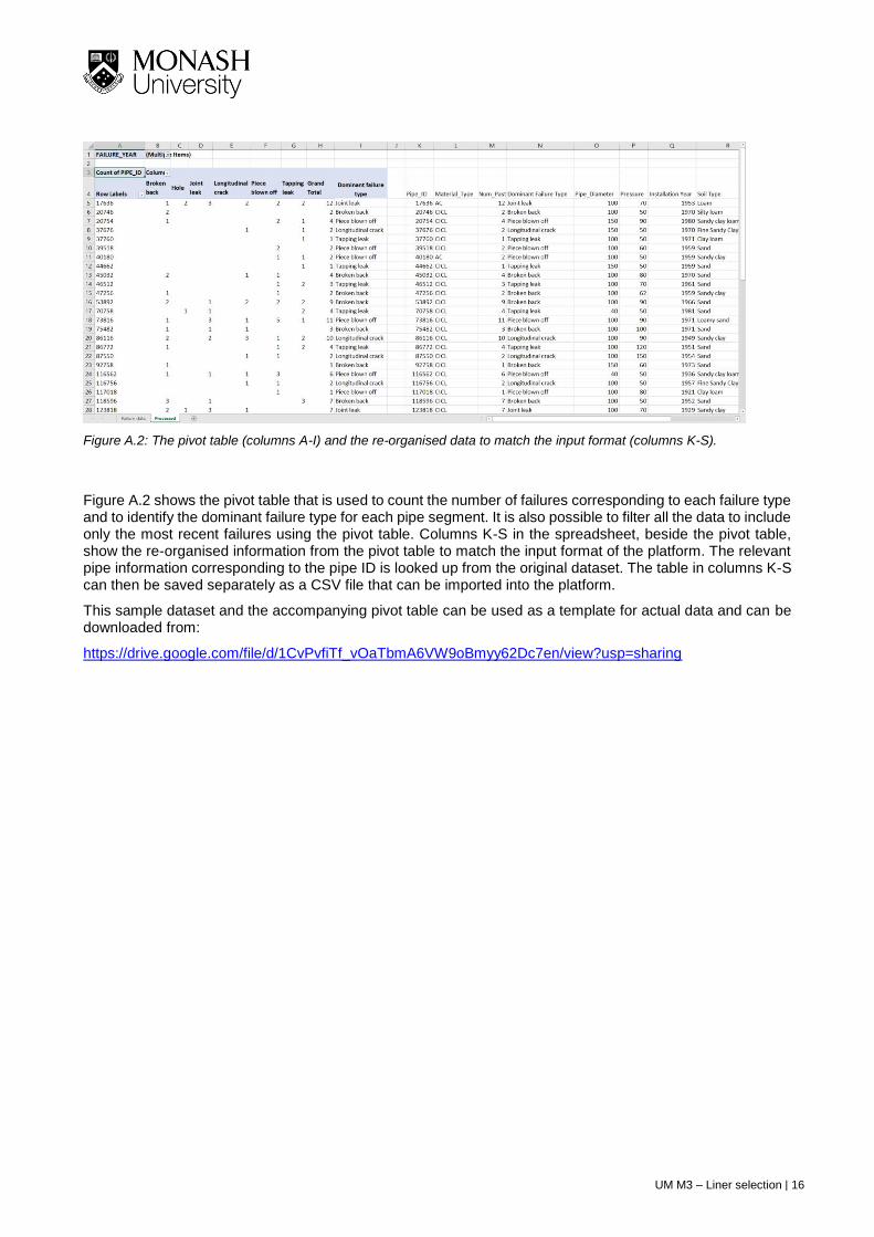
Figure A.2: The pivot table (columns A-I) and the re-organised data to match the input format (columns K-S).

Figure A.2 shows the pivot table that is used to count the number of failures corresponding to each failure type and to identify the dominant failure type for each pipe segment. It is also possible to filter all the data to include only the most recent failures using the pivot table. Columns K-S in the spreadsheet, beside the pivot table, show the re-organised information from the pivot table to match the input format of the platform. The relevant pipe information corresponding to the pipe ID is looked up from the original dataset. The table in columns K-S can then be saved separately as a CSV file that can be imported into the platform.

This sample dataset and the accompanying pivot table can be used as a template for actual data and can be downloaded from:

https://drive.google.com/file/d/1CvPvfiTf_vOaTbmA6VW9oBmyy62Dc7en/view?usp=sharing

https://drive.google.com/file/d/1CvPvfiTf_vOaTbmA6VW9oBmyy62Dc7en/view?usp=sharing


Method 2: Using a Python script

A Python script has been written to count and re-organise the utility raw data into the required input format similar to the pivot table. In addition, this script also checks for any spelling variants or different naming conventions for the different failure types. A dictionary file with the most common variants of the failure types is used to homogenise the input data and convert them to a common format. For example, this means that variations such as B/Back, BB, BrBack, circumferential failure and including minor spelling errors are all identified as a Broken back failure. The dictionary file can be updated based on utility requirements for more flexibility.

The script has been organised as a function that takes the source data as a Pandas dataframe and the past number of years that need to be considered in filtering as inputs. The function returns a CSV file formatted into the correct format. The python code can be run in a Jupyter notebook and can be downloaded along with the dictionary file from:

https://drive.google.com/drive/folders/18_wCCgt1x0-OyxWk5_lGYu0qgmaLtUwX?usp=sharing

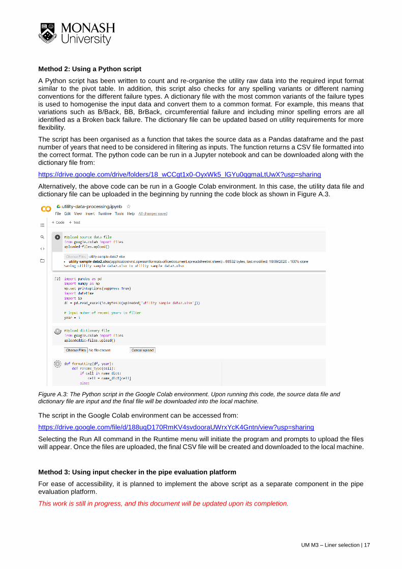
Alternatively, the above code can be run in a Google Colab environment. In this case, the utility data file and dictionary file can be uploaded in the beginning by running the code block as shown in Figure A.3.

Figure A.3: The Python script in the Google Colab environment. Upon running this code, the source data file and dictionary file are input and the final file will be downloaded into the local machine.

The script in the Google Colab environment can be accessed from:

https://drive.google.com/file/d/188uqD170RmKV4svdooraUWrxYcK4Gntn/view?usp=sharing

Selecting the Run All command in the Runtime menu will initiate the program and prompts to upload the files will appear. Once the files are uploaded, the final CSV file will be created and downloaded to the local machine.

Method 3: Using input checker in the pipe evaluation platform

For ease of accessibility, it is planned to implement the above script as a separate component in the pipe evaluation platform.

This work is still in progress, and this document will be updated upon its completion.

https://drive.google.com/drive/folders/18_wCCgt1x0-OyxWk5_lGYu0qgmaLtUwX?usp=sharing

https://drive.google.com/file/d/188uqD170RmKV4svdooraUWrxYcK4Gntn/view?usp=sharing

Documents

User Manual Module 3 Liner selection