Embed Size (px)
Citation preview
DosiVox-2DUser Manual
Loïc Martin & Norbert MercierIRAMAT-CRP2A
Université Bordeaux MontaigneMaison de l'Archéologie, Esplanade des Antilles
33607 Pessac Cedex, France

For technical support, please contact :
Loïc MARTIN: [email protected] MERCIER: [email protected]
DosiVox-2D and corresponding documentation are available at http://www.iramat-crp2a.cnrs.fr/spip/spip.php?article144.
Table of Contents
1 – Introduction…………………………………………………….…... p.2
2 – Installation ………………………………………………………… p.5
3 – Create a modelling …………………………………………….. p.6
4 – Running a simulation …………………………………………….. p.16
5 – Results processing ….…………………………………………. p.19
6 – References ………………………………………………………… p.22
1
1 – IntroductionPrinciples
DosiVox-2D is a software designed to simulate the beta radioactivity and calculate dose rate in heterogeneousisotropic samples of rocks or sediments (Martin et al., 2018; Fang et al., 2018). It can be freely downloaded with its Javainterface and documentation at http://www.iramat-crp2a.cnrs.fr/spip/spip.php?article144. It is derivated from DosiVox(Martin et al., 2015a, Martin et al., 2015b, Martin et al., 2015c, http://www.iramat-crp2a.cnrs.fr/spip/spip.php?article144 ),both created with the Geant4 toolkit (Agostinelli et al., 2003; Allison et al., 2007). DosiVox-2D is based on the concept of2D-modelling, in which beta particles are simulated in a flat representation of the sample. The software provides at the endof the calculations the distribution of beta dose rates in the different material/mineral modeled phases, as well as averagevalues.
In DosiVox-2D, one constructs the 2D-modelling from a segmented 2D-mapping of a sample, representing thedifferent materials composing this sample. Each pixel of the image becomes a voxel of the modelling, containing theinformation related to its constituting material (chemical composition, density, moisture, radioactive element contents); thevoxel is also able to record doses, what finally allows to calculate dose rates. The software runs the simulation of the betaparticle emissions coming from the K or/and U-series or/and Th-series. Alpha and gamma spectra are also available but nottested for 2D-modelling. As detailled in Martin (2015): the alpha particle specta (Uapha, Thalpha) are constructed from theNIST online database (Kramida et al., 2018); the beta particle spectra (Ubeta, Thbeta, Kbeta) and the gamma particlespectra (Ugamma, Thgamma) are based on the data from the NNDC (Brookhaven National Laboratory, USA,http://www.nndc.bnl.gov/) online database NuDat (version nov 2009)(Kinsey et al., 1996). In addition, the K gammaspectra (Kgamma) is constructed from NNDC online database NuDat (version janv 2013)(Kinsey et al., 1996). It is alsopossible to use your own energy spectrum for the beta particle emissions, referred as “User-defined” or "Udef". The resultsare provided as average dose rate in the sample, average dose rate in each material/mineral fraction represented, basichistograms of dose rate distributions for the different elements simulated and for each material, and beta dose rate mappingsfor the whole sample. The 2D-modelling simulations have been demonstrated to be equivalent to those of standard 3Dmodellings (Martin et al., 2018) in the limit of representativeness of the modeled slice over the whole sample.
Requirements
The following list contains the basic data and unavoidable considerations to create 2D-modellings with DosiVox-2D. It isimportant to keep in mind that a modelling is not a perfect representation of the reality, but is circumscribed by theuncertainty on the different parameters and approximations made by the user. Thus, it is possible to construct very accurateand heavy modellings with detailed data, or basic and fast simulations with only the minimum data required. It can be alsouseful to perform series of simulations with different values for a single parameter (like the moisture), in order tocharacterize the range of possible dose rates. All these ways to use the 2D-modelling (and any modelling in general) arecorrect and consistent inside the limits of the accuracy of your parameters and the assumptions made.
first of all, you need to consider that DosiVox-2D applies only to isotropic samples, i.e. a sample where thedistribution of the different materials/grains/heterogeneities is similar, in terms of probability, in all directions(Underwood, 1970; Martin et al., 2018). Without this condition, the 2D-mapping of the sample cannot beconsidered as representative of the whole sample (Fang et al., 2018). The isotropic condition must be consideredonly at the beta particle scale (millimeter to centimeter), what means that a layer (for instance a sedimentary layer)can be locally isotropic if the different objects and materials composing it are heterogeneous but well mixedtogether, and even if this layer is actually an anisotropic object by definition. In this case, 2D-modelling can beperformed on a sample slice included in the layer under study. The crucial point is to get a sample slice for the 2D-mapping that can be considered as representative of the whole sample, in terms of material proportions anddistributions. It is noticeable that 2D-modelling seems to give reliable results as well, even if a slight anisotropycan be observed, like a preferential direction of mineralization (Fang et al., 2018).
2
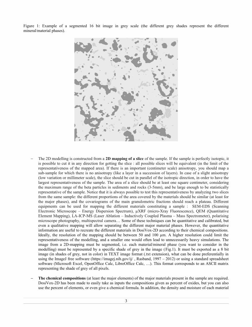
Figure 1: Example of a segmented 16 bit image in grey scale (the different grey shades represent the differentmineral/material phases).
The 2D modelling is constructed from a 2D mapping of a slice of the sample. If the sample is perfectly isotopic, itis possible to cut it in any direction for getting the slice : all possible slices will be equivalent (in the limit of therepresentativeness of the mapped area). If there is an important (centimeter scale) anisotropy, you should map asub-sample for which there is no anisotropy (like a layer in a succession of layers). In case of a slight anisotropy(low variation or millimeter scale), the slice should be cut in parallel of the isotropic direction, in order to have thelargest representativeness of the sample. The area of a slice should be at least one square centimeter, consideringthe maximum range of the beta particles in sediments and rocks (3-5mm), and be large enough to be statisticallyrepresentative of the sample. Notice that it is always possible to test this representativeness by analyzing two slicesfrom the same sample: the different proportions of the area covered by the materials should be similar (at least forthe major phases), and the covariograms of the main granulometric fractions should reach a plateau. Differentequipments can be used for mapping the different materials constituting a sample : SEM-EDS (ScanningElectronic Microscope – Energy Dispersion Spectrum), µXRF (micro-Xray Fluorescence), QEM (QuantitativeElement Mapping), LA-ICP-MS (Laser Ablation – Inductively Coupled Plasma – Mass Spectrometer), polarisingmicroscope photography, multispectral camera… Some of these techniques can be quantitative and calibrated, buteven a qualitative mapping will allow separating the different major material phases. However, the quantitativeinformation are useful to recreate the different materials in DosiVox-2D according to their chemical compositions.Ideally, the resolution of the mapping should be between 50 and 100 µm. A higher resolution could limit therepresentativeness of the modelling, and a smaller one would often lead to unnecessarily heavy simulations. Theimage from a 2D-mapping must be segmented, i.e. each material/mineral phase (you want to consider in themodelling) must be represented by a specific shade of grey in the image (Fig.1). It must be exported as a 8 bitimage (in shades of grey, not in color) in TEXT image format (.txt extension), what can be done preferentially inusing the ImageJ free software (https://imagej.nih.gov/ij/ , Rasband, 1997 – 2012) or using a standard spreadsheetsoftware (Microsoft Excel, OpenOffice Calc, LibreOffice Calc, …). This format corresponds to an ASCII matrixrepresenting the shade of grey of all pixels.
The chemical compositions (at least the major elements) of the major materials present in the sample are required.DosiVox-2D has been made to easily take as inputs the compositions given as percent of oxides, but you can alsouse the percent of elements, or even give a chemical formula. In addition, the density and moisture of each material
3
must be given. These data are somewhat difficult to get in case of loose materials, but it is usually possible toestimate these values and test various set of parameters. You might often consider only the major material phases,but other phases could be very important as well (if their radioactivity is significantly higher than the rest of thesample, like K-feldspars or zircons). A quick way to judge if a minor material must be represented or not is toestimate the proportion of beta dose from this material in the sample. Simply multiply the estimated massproportion of the material by its estimated radioactive content and by the corresponding beta dose conversionfactor. If both the resulting dose rate, normalized to the infinite matrix beta dose rate, and the mass proportion ofthe material are lower than one percent, the material can likely be neglected in the modelling.
You need to define the contents of radioactive elements (K, U-series, Th-series or/and user defined betaspectrum) for each modelled material. It is possible afterwards to adjust manually these values in each voxel.DosiVox-2D provides the beta energy spectrum of the K, the U-series and the Th-series (both at secularequilibrium). A user defined file is available in the software folder (DosiVox-2D/data/spectra/Userdef.txt) forimplementing your own energy spectrum (for example a U-series spectrum in disequilibrium), following thedefined pattern : the first line contains the conversion factor from element content to dose rate (Gray/ka) followedby a description ; then, a first column lists the energies of the emitted beta particles (in keV) and a second columngives the cumulative probabilities of these energies. The contents of the different radioactive elements can usuallybe obtained by LA-ICP-MS measurements, or mineral separation followed by ICP-MS or gamma spectrometrymeasurements. It is also possible to get the K content directly with the slice mapping analysis if a quantitativecalibration is set, and possibly the U and Th contents if they are high enough. If the access to these measurementfacilities is limited, you might consider the K, U and Th contents from the bulk sample, and test differenthypotheses of their distribution in the different materials.
you need to have the DosiVox-2D software installed (This software runs on Linux systems and has beenspecifically precompiled and tested for the Linux virtual machine available atftp://ftp.cenbg.in2p3.fr/info/Vmware/Old-Versions/g4.10.01.p01/ , see part 2), and a Java environment set forrunning the graphical interface (if you choose to run the software under the proposed virtual machine, the Javaenvironment is already set inside).
→ To sum up, once you have checked that your sample is isotropic (or almost) at the scale of the beta dose rateheterogeneity, you need, in order to perform a 2D-modelling with DosiVox-2D, to make a material mapping from a sliceof the sample, know the composition of the different major material phases as well as their contents in radioactiveelements, and of course have DosiVox-2D and its interface installed.
4
2 – InstallationThe DosiVox-2D software works under Linux. It was developed and tested with Scientific Linux 6.4 (Red HatTM),
running on the Geant4 Virtual Machine (freely available at: ftp://ftp.cenbg.in2p3.fr/info/Vmware/Old-Versions/g4.10.01.p01/ ) developped by the Centre d'Etudes Nucléaires de Bordeaux-Gradignan, France ( Incerti et al.,2010). This virtual machine itself contains the Geant4 libraries, which are necessary for compiling the source code, if non-compilated or modifed DosiVox-2D codes are used.
The provided instructions are given for a PC with the following setup:# Windows 7, 64 bit# Memory: min. 4 GB
1 – Download the virtual machine and unzip it in a folder.
2 – Installing the virtual machine playerDosiVox was tested with VMwareTM Workstation 12 Player (free for PC) and VMware Fusion 6TM (available for purchasefor Mac).
3 – Opening the virtual machineRun the virtual machine player and choose to open a Virtual Machine (browse and select the file sl6 x64:vmdk). Play thevirtual machine. The Parameters of this machine can be modified by editing virtual machine settings. For furtherinformation the user is invited to read the README file on the : ftp://ftp.cenbg.in2p3.fr/info/Vmware/Old-Versions/g4.10.01.p01/ page.
Note: At the first virtual machine start, VMware Player displays a message asking whether you have moved or copied thevirtual machine. You have to answer "I copied it".
Note: The virtual machine works as an independant computer on the user PC or Mac. All the data in the virtual machineare not automaticly saved in the regular computer, for example in the case of the deleting of the virtual machine. To accessand save virtual machine data outside of the virtual machine (simulation results for example), use a shared folder betweenthe regular computer and the virtual machine, or copy the data files in the virtual machine and paste them on the regularcomputer.
4 – Download and unzip the DosiVox-2D folder The DosiVox-2D folder contains three sub-folders: build, data, results.
The data folder contains the spectra folder where all the spectra used for simulations are stored. All these files are TXTfiles and therefore can be easily modified. For instance, the file UserDef allows the user to simulate any particle, includingones other than those emitted by the 40K and U- and Th-series. The data folder must also contain the Pilot Text Files (PTF)used by Geant4 to run the simulations (cf. DosiVox manual for further information on the PTFs).The results folder containsthe results of the simulation (cf. DosiVox manual for further information).
5 – Copy and paste the DosiVox-2D folder in the virtual machine /local1 folderIf you unzip the DosiVox-2D folder directly under the virtual machine, the access to the file may be restricted by Linux forsecurity. To allow accessing the files and launching the simulations, right-click on the DosiVox-2D folder icon, go in“properties” and select the options « Allow executing file as program » and « Apply permissions to enclosed files » in the“permissions” tabulation.
6 – DosiVox-2D is now ready to work. Follow the manual in order to build and run a modelling with it.
5
3 – Create a modellingThe graphical interface DosiEdit2D
DosiEdit2D is a user-friendly Java Graphical User Interface (GUI) for creating DosiVox-2D simulations. You cannot directly run a simulation from it, but it allows creating a Pilot Text File (PTF), as for DosiVox (Martin et al., 2015a).This interface run on any computer with a Java (8 or superior) environment set. To launch it, double-click on theDosiEdit2D.jar file. Notice that a Visual Basic interface is also available at http://www.iramat-crp2a.cnrs.fr/spip/spip.php?article144.
Open/load a new project
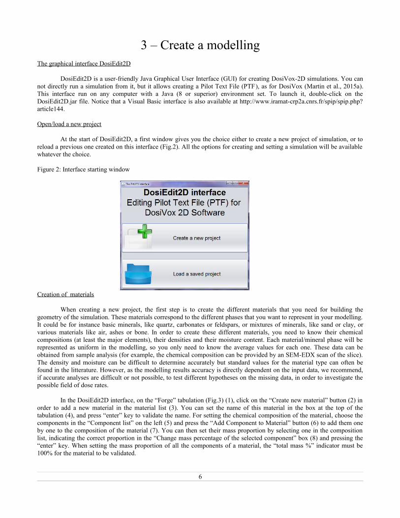
At the start of DosiEdit2D, a first window gives you the choice either to create a new project of simulation, or toreload a previous one created on this interface (Fig.2). All the options for creating and setting a simulation will be availablewhatever the choice.
Figure 2: Interface starting window
Creation of materials
When creating a new project, the first step is to create the different materials that you need for building thegeometry of the simulation. These materials correspond to the different phases that you want to represent in your modelling.It could be for instance basic minerals, like quartz, carbonates or feldspars, or mixtures of minerals, like sand or clay, orvarious materials like air, ashes or bone. In order to create these different materials, you need to know their chemicalcompositions (at least the major elements), their densities and their moisture content. Each material/mineral phase will berepresented as uniform in the modelling, so you only need to know the average values for each one. These data can beobtained from sample analysis (for example, the chemical composition can be provided by an SEM-EDX scan of the slice).The density and moisture can be difficult to determine accurately but standard values for the material type can often befound in the litterature. However, as the modelling results accuracy is directly dependent on the input data, we recommend,if accurate analyses are difficult or not possible, to test different hypotheses on the missing data, in order to investigate thepossible field of dose rates.
In the DosiEdit2D interface, on the “Forge” tabulation (Fig.3) (1), click on the “Create new material” button (2) inorder to add a new material in the material list (3). You can set the name of this material in the box at the top of thetabulation (4), and press “enter” key to validate the name. For setting the chemical composition of the material, choose thecomponents in the “Component list” on the left (5) and press the “Add Component to Material” button (6) to add them oneby one to the composition of the material (7). You can then set their mass proportion by selecting one in the compositionlist, indicating the correct proportion in the “Change mass percentage of the selected component” box (8) and pressing the“enter” key. When setting the mass proportion of all the components of a material, the “total mass %” indicator must be100% for the material to be validated.
6
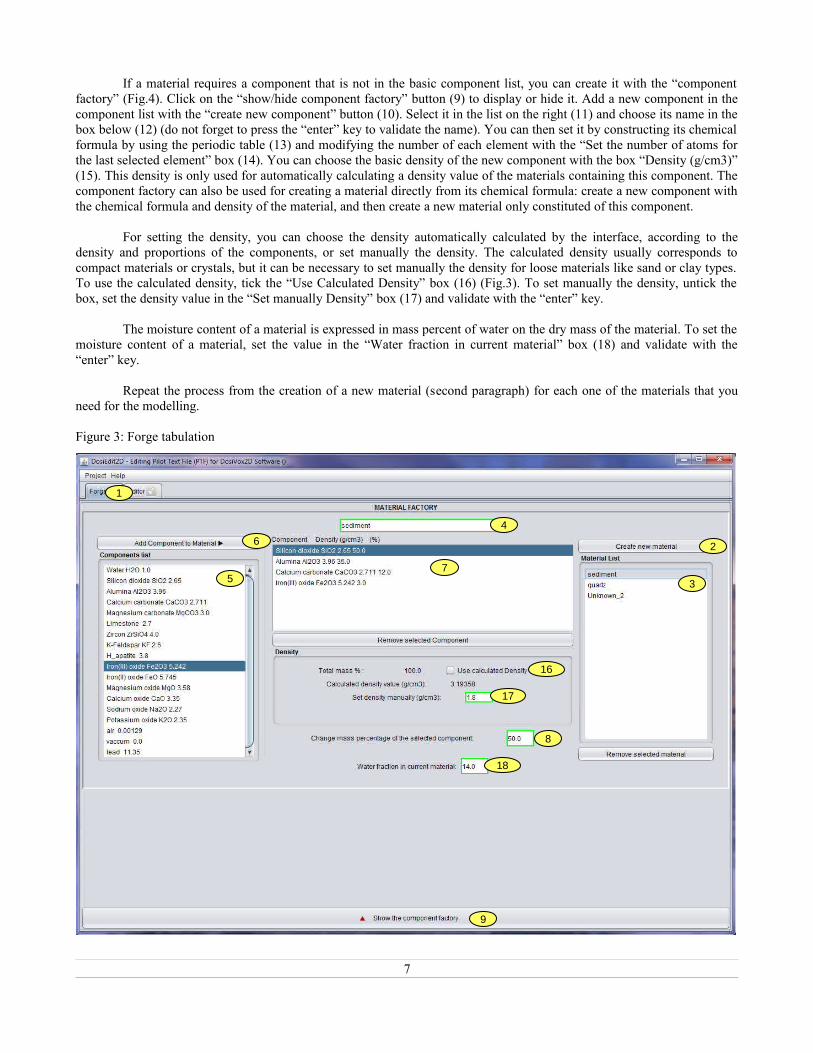
If a material requires a component that is not in the basic component list, you can create it with the “componentfactory” (Fig.4). Click on the “show/hide component factory” button (9) to display or hide it. Add a new component in thecomponent list with the “create new component” button (10). Select it in the list on the right (11) and choose its name in thebox below (12) (do not forget to press the “enter” key to validate the name). You can then set it by constructing its chemicalformula by using the periodic table (13) and modifying the number of each element with the “Set the number of atoms forthe last selected element” box (14). You can choose the basic density of the new component with the box “Density (g/cm3)”(15). This density is only used for automatically calculating a density value of the materials containing this component. Thecomponent factory can also be used for creating a material directly from its chemical formula: create a new component withthe chemical formula and density of the material, and then create a new material only constituted of this component.
For setting the density, you can choose the density automatically calculated by the interface, according to thedensity and proportions of the components, or set manually the density. The calculated density usually corresponds tocompact materials or crystals, but it can be necessary to set manually the density for loose materials like sand or clay types.To use the calculated density, tick the “Use Calculated Density” box (16) (Fig.3). To set manually the density, untick thebox, set the density value in the “Set manually Density” box (17) and validate with the “enter” key.
The moisture content of a material is expressed in mass percent of water on the dry mass of the material. To set themoisture content of a material, set the value in the “Water fraction in current material” box (18) and validate with the“enter” key.
Repeat the process from the creation of a new material (second paragraph) for each one of the materials that youneed for the modelling.
Figure 3: Forge tabulation
7
1
2
3
4
5
6
7
8
9
16
17
18
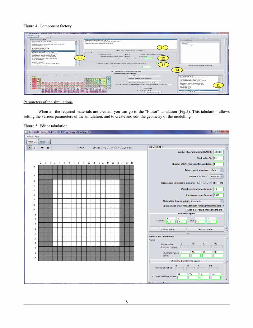
Figure 4: Component factory
Parameters of the simulations
When all the required materials are created, you can go to the “Editor” tabulation (Fig.5). This tabulation allowssetting the various parameters of the simulation, and to create and edit the geometry of the modelling.
Figure 5: Editor tabulation
8
10
12
11
13
14
15
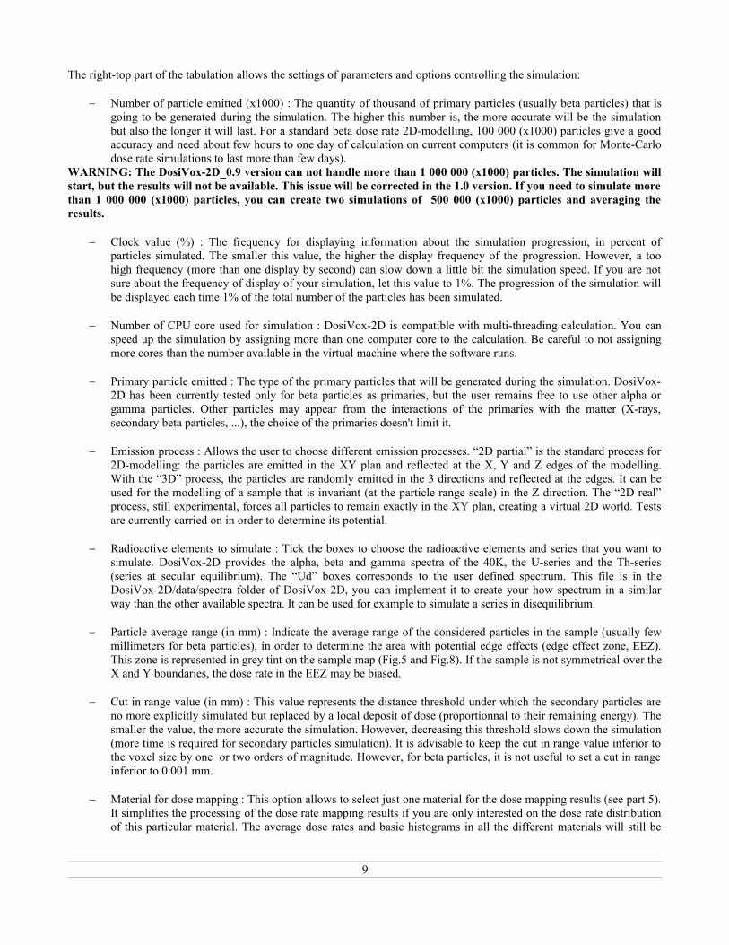
The right-top part of the tabulation allows the settings of parameters and options controlling the simulation:
Number of particle emitted (x1000) : The quantity of thousand of primary particles (usually beta particles) that isgoing to be generated during the simulation. The higher this number is, the more accurate will be the simulationbut also the longer it will last. For a standard beta dose rate 2D-modelling, 100 000 (x1000) particles give a goodaccuracy and need about few hours to one day of calculation on current computers (it is common for Monte-Carlodose rate simulations to last more than few days).
WARNING: The DosiVox-2D_0.9 version can not handle more than 1 000 000 (x1000) particles. The simulation willstart, but the results will not be available. This issue will be corrected in the 1.0 version. If you need to simulate morethan 1 000 000 (x1000) particles, you can create two simulations of 500 000 (x1000) particles and averaging theresults.
Clock value (%) : The frequency for displaying information about the simulation progression, in percent ofparticles simulated. The smaller this value, the higher the display frequency of the progression. However, a toohigh frequency (more than one display by second) can slow down a little bit the simulation speed. If you are notsure about the frequency of display of your simulation, let this value to 1%. The progression of the simulation willbe displayed each time 1% of the total number of the particles has been simulated.
Number of CPU core used for simulation : DosiVox-2D is compatible with multi-threading calculation. You canspeed up the simulation by assigning more than one computer core to the calculation. Be careful to not assigningmore cores than the number available in the virtual machine where the software runs.
Primary particle emitted : The type of the primary particles that will be generated during the simulation. DosiVox-2D has been currently tested only for beta particles as primaries, but the user remains free to use other alpha orgamma particles. Other particles may appear from the interactions of the primaries with the matter (X-rays,secondary beta particles, ...), the choice of the primaries doesn't limit it.
Emission process : Allows the user to choose different emission processes. “2D partial” is the standard process for2D-modelling: the particles are emitted in the XY plan and reflected at the X, Y and Z edges of the modelling.With the “3D” process, the particles are randomly emitted in the 3 directions and reflected at the edges. It can beused for the modelling of a sample that is invariant (at the particle range scale) in the Z direction. The “2D real”process, still experimental, forces all particles to remain exactly in the XY plan, creating a virtual 2D world. Testsare currently carried on in order to determine its potential.
Radioactive elements to simulate : Tick the boxes to choose the radioactive elements and series that you want tosimulate. DosiVox-2D provides the alpha, beta and gamma spectra of the 40K, the U-series and the Th-series(series at secular equilibrium). The “Ud” boxes corresponds to the user defined spectrum. This file is in theDosiVox-2D/data/spectra folder of DosiVox-2D, you can implement it to create your how spectrum in a similarway than the other available spectra. It can be used for example to simulate a series in disequilibrium.
Particle average range (in mm) : Indicate the average range of the considered particles in the sample (usually fewmillimeters for beta particles), in order to determine the area with potential edge effects (edge effect zone, EEZ).This zone is represented in grey tint on the sample map (Fig.5 and Fig.8). If the sample is not symmetrical over theX and Y boundaries, the dose rate in the EEZ may be biased.
Cut in range value (in mm) : This value represents the distance threshold under which the secondary particles areno more explicitly simulated but replaced by a local deposit of dose (proportionnal to their remaining energy). Thesmaller the value, the more accurate the simulation. However, decreasing this threshold slows down the simulation(more time is required for secondary particles simulation). It is advisable to keep the cut in range value inferior tothe voxel size by one or two orders of magnitude. However, for beta particles, it is not useful to set a cut in rangeinferior to 0.001 mm.
Material for dose mapping : This option allows to select just one material for the dose mapping results (see part 5).
It simplifies the processing of the dose rate mapping results if you are only interested on the dose rate distributionof this particular material. The average dose rates and basic histograms in all the different materials will still be
9
provided in the main result file, but the voxels filled by the no-selected materials will get the default value “0” inthe dose rate mappings results. If you prefer to get the dose rate mapping in all the materials, just let this option to“All materials”. You will still be able to separate the dose rate mapping of the different materials with a few imageprocessing (see part 5).
Exclude edge effect zones for dose results (recommended): this option excludes the voxels in the EEZ for the doserate calculation and mapping in the result files. It avoids potential bias in the results due to a local break of theisotropy of the modelling at the edges. However, if you want to include these voxels in the results (in the casewhere you are sure that the statistical isotropy of the modelling is respected), uncheck this box.
The “Voxel description” box (Fig.5) is used to set the size of the voxel grid. The size of the voxel in the X and Ydirection, corresponding to the resolution of the 2D image in these directions, have to be provided here. Thenumber of voxels can be used to modify the voxel grid size when creating manually a 2D geometry, but is uselesswhen loading a 2D image (which is the standard way of using DosiEdit2D).
Do not forget to press the “enter” key to validate any input. You can also use the “Validate values” button tovalidate all the changes. The “Refresh values” button applies the changes to the voxel mapping when applicable.
We strongly advise you to save the project at this point, before loading a 2D image. Even if a project with an imagecan be saved, the saved file might be heavy and its reloading might be long and memory consuming. A project savedwithout an image allows to reload all the created materials and all the set parameters. To save the project, click on the“Project” menu at the top left of the interface, and choose “save” or “save as”.
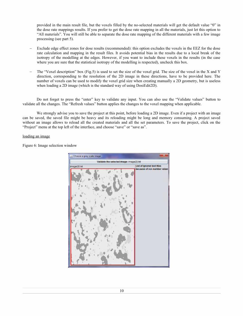
loading an image
Figure 6: Image selection window
10
For building the geometry of your sample in the modelling, you have to load a 2D 8bit image in shades of grey.This image has to be segmented, meaning that each material/mineral is represented by one specific grey shade. The imagemust be in TXT format (available from standard spreadsheet softwares or the free image processing software ImageJ, seeRasband, 1997 – 2012).
For loading an image, click on the “Load a grey scale image into the grid” button, and then select the foldercontaining the image. A window displaying the different images available in this folder will appear in the interface (Fig.6).From it, you can select the image (Fig.1) by clicking on it and then clicking on the “Validate the select image” button at thetop of the window.
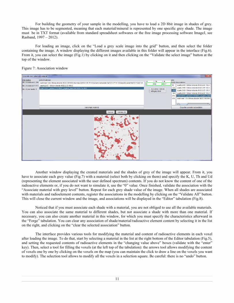
Figure 7: Association window
Another window displaying the created materials and the shades of grey of the image will appear. From it, youhave to associate each grey value (Fig.7) with a material (select both by clicking on them) and specify the K, U, Th and Ud(representing the element associated with the user defined spectrum) contents. If you do not know the content of one of theradioactive elements or, if you do not want to simulate it, use the “0” value. Once finished, validate the association with the“Associate material with grey level” button. Repeat for each grey shade value of the image. When all shades are associatedwith materials and radioelement contents, register the associations in the modelling by clicking on the “Validate All” button.This will close the current window and the image, and associations will be displayed in the “Editor” tabulation (Fig.8).
Noticed that if you must associate each shade with a material, you are not obliged to use all the available materials.You can also associate the same material to different shades, but not associate a shade with more than one material. Ifnecessary, you can also create another material in this window, for which you must specify the characteristics afterward inthe “Forge” tabulation. You can clear any association of shade/material/radioactive element content by selecting it in the liston the right, and clicking on the “clear the selected association” button.
The interface provides various tools for modifying the material and content of radioactive elements in each voxelafter loading the image. To do that, start by selecting a material in the list at the right bottom of the Editor tabulation (Fig.5),and setting the requested contents of radioactive elements in the “changing value above” boxes (validate with the “enter”key). Then, select a tool for filling the voxels (at the left top of the tabulation): the arrows tool allows modifying the contentof voxels one by one by clicking on the voxels on the map (you can maintain the click to draw a line on the voxels you wantto modify). The selection tool allows to modify all the voxels in a selection square. Be careful: there is no “undo” button.
11
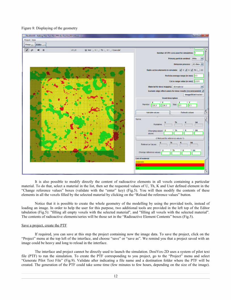
Figure 8: Displaying of the geometry
It is also possible to modify directly the content of radioactive elements in all voxels containing a particularmaterial. To do that, select a material in the list, then set the requested values of U, Th, K and User defined element in the“Change reference values” boxes (validate with the “enter” key) (Fig.5). You will then modify the contents of theseelements in all the voxels filled by the selected material by clicking on the “Reload the reference values” button.
Notice that it is possible to create the whole geometry of the modelling by using the provided tools, instead ofloading an image. In order to help the user for this purpose, two additional tools are provided in the left top of the Editortabulation (Fig.5): "filling all empty voxels with the selected material", and "filling all voxels with the selected material".The contents of radioactive elements/series will be those set in the “Radioactive Element Contents” boxes (Fig.5).
Save a project, create the PTF
If required, you can save at this step the project containing now the image data. To save the project, click on the“Project” menu at the top left of the interface, and choose “save” or “save as”. We remind you that a project saved with animage could be heavy and long to reload in the interface.
The interface and project cannot be directly used to launch the simulation. DosiVox-2D uses a system of pilot textfile (PTF) to run the simulation. To create the PTF corresponding to you project, go to the “Project” menu and select“Generate Pilot Text File” (Fig.9). Validate after indicating a file name and a destination folder where the PTF will becreated. The generation of the PTF could take some time (few minutes to few hours, depending on the size of the image).
12
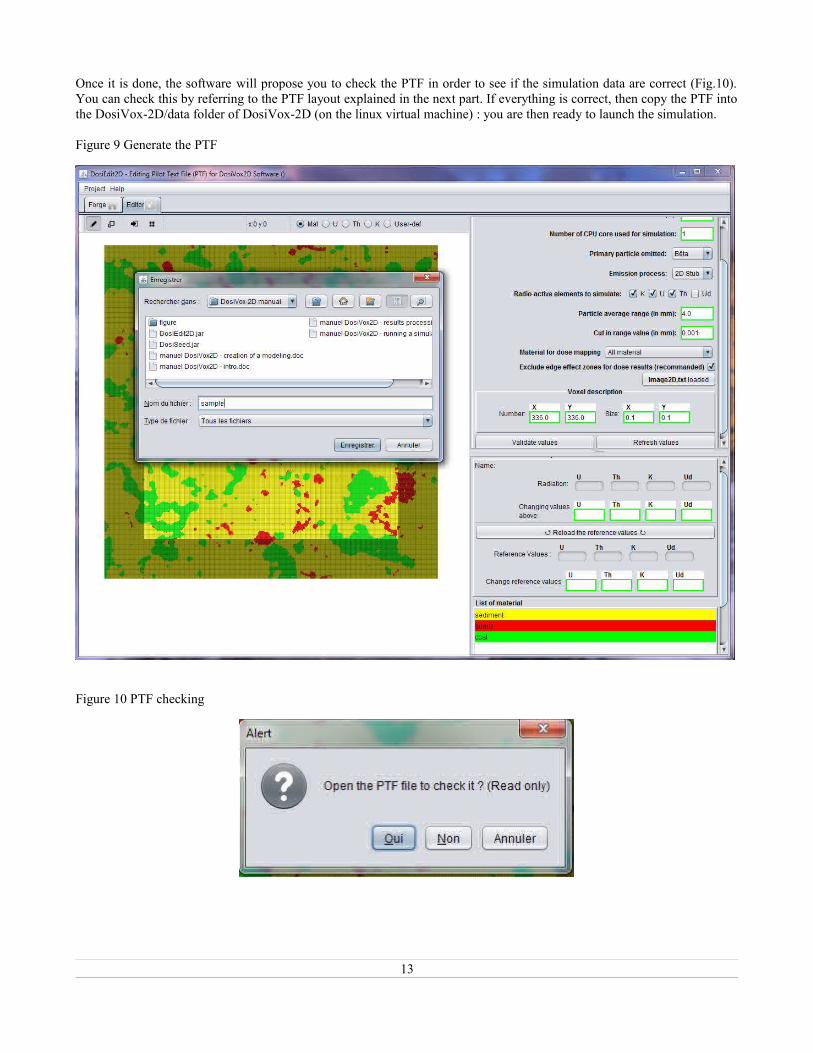
Once it is done, the software will propose you to check the PTF in order to see if the simulation data are correct (Fig.10).You can check this by referring to the PTF layout explained in the next part. If everything is correct, then copy the PTF intothe DosiVox-2D/data folder of DosiVox-2D (on the linux virtual machine) : you are then ready to launch the simulation.
Figure 9 Generate the PTF
Figure 10 PTF checking
13
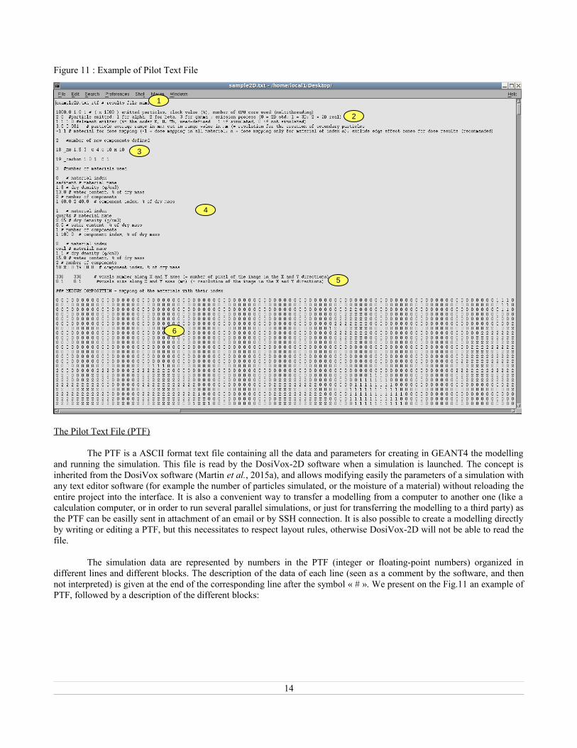
Figure 11 : Example of Pilot Text File
The Pilot Text File (PTF)
The PTF is a ASCII format text file containing all the data and parameters for creating in GEANT4 the modellingand running the simulation. This file is read by the DosiVox-2D software when a simulation is launched. The concept isinherited from the DosiVox software (Martin et al., 2015a), and allows modifying easily the parameters of a simulation withany text editor software (for example the number of particles simulated, or the moisture of a material) without reloading theentire project into the interface. It is also a convenient way to transfer a modelling from a computer to another one (like acalculation computer, or in order to run several parallel simulations, or just for transferring the modelling to a third party) asthe PTF can be easilly sent in attachment of an email or by SSH connection. It is also possible to create a modelling directlyby writing or editing a PTF, but this necessitates to respect layout rules, otherwise DosiVox-2D will not be able to read thefile.
The simulation data are represented by numbers in the PTF (integer or floating-point numbers) organized indifferent lines and different blocks. The description of the data of each line (seen as a comment by the software, and thennot interpreted) is given at the end of the corresponding line after the symbol « # ». We present on the Fig.11 an example ofPTF, followed by a description of the different blocks:
14
1
2
3
4
5
6
− The first line of the PTF (1) is the name for the results file (or RTF, see part X).
− The first block contains data relative to the general parameters of the simulation (2), like the number andtype of the particles to generate, or the radioactive element and/or series to simulate.
− The following series of blocks describes the new components, if any were created by the user (3). Eachone is characterized by an index (starting at 18, because indexes 0 to 17 correspond to the basiccomponents available in the interface, see Fig.3-(5)), its name, its density (only used in the interface forcalculating the default density of the materials containing it), and the number of elements it contains,followed by the list of symbols and numbers of atoms of each element composing it.
− The second series of blocks describes the different materials filling the voxels (4). Each one ischaracterized by an index, allowing to represent it in the material mapping: its name, its density, itsmoisture content, and the number, indexes and proportions of its components.
− After the material description, a data block defines the voxel grid where the sample is represented (voxelsizes and numbers in the X and Y direction) (5).
− The first matrix below is the material mapping (6). It is a matrix representing the material filling eachvoxel of the grid. This matrix has the size of the grid (the lines and columns represent respectively the Xand Y axis, each value represents a voxel) and each material is represented by its index issued from thedata blocks of material description.
− The four following matrices, sharing the same layout than the material mapping matrix, represent themapping of the radioactive contents. The order of the matrices is 40K, U-series, Th-series and UserDefined element.
It is possible to edit (or create, for experimented users) a PTF with a text editor software. Please find below some rules andadvices:
◦You must respect the layout and the order of the data blocks presented above.
◦ The data blocks, the components and the materials must be separated by one and only one empty line
◦ The data in a line must be separated by at least one space. Avoid using tabulation.
◦ The decimal separator is the point. Do not use comma.
◦Do not use complex notation for numbers (with power of ten for example).
◦ The indexes of the new components starts at “18”, those of the material at “0”.
◦ The unit of the U, Th and Udef mapping is ppm. The unit of the K mapping is %.
15
4 – Running a simulationLaunching a simulation
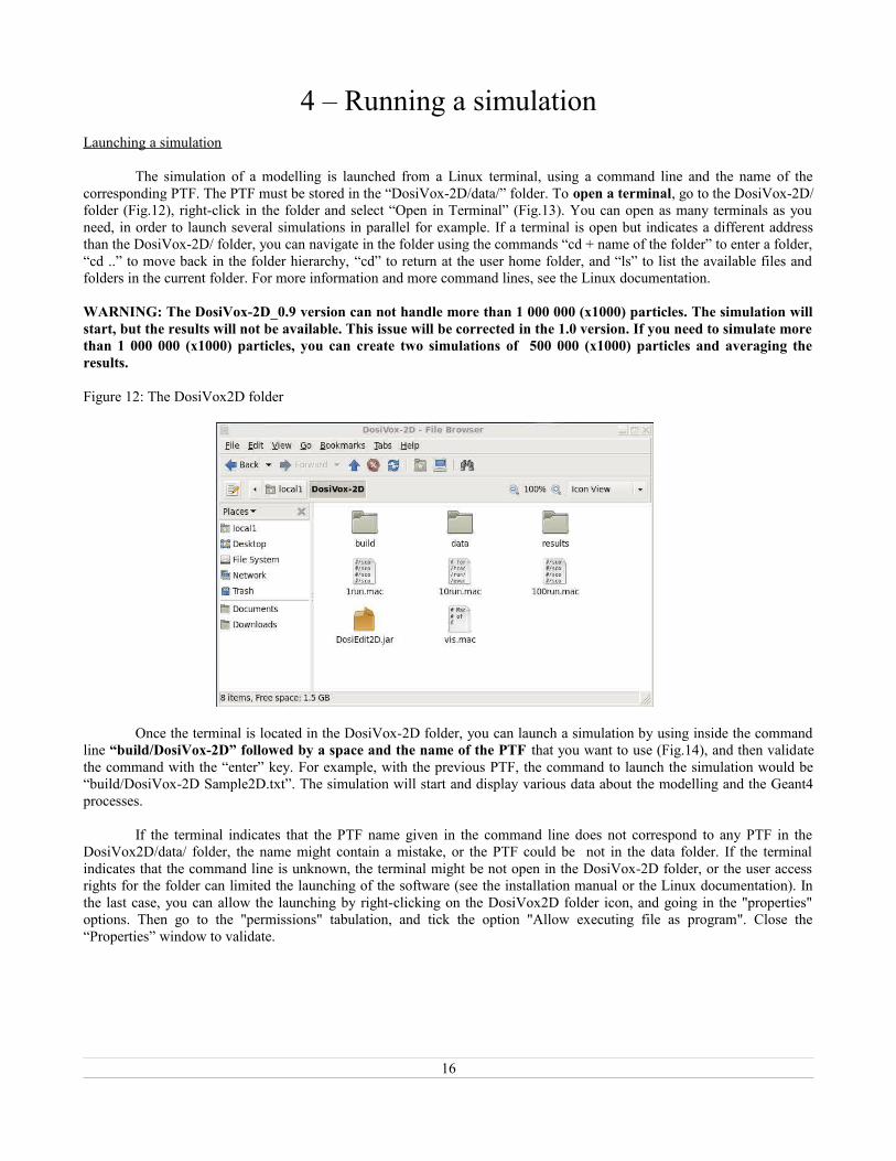
The simulation of a modelling is launched from a Linux terminal, using a command line and the name of thecorresponding PTF. The PTF must be stored in the “DosiVox-2D/data/” folder. To open a terminal, go to the DosiVox-2D/folder (Fig.12), right-click in the folder and select “Open in Terminal” (Fig.13). You can open as many terminals as youneed, in order to launch several simulations in parallel for example. If a terminal is open but indicates a different addressthan the DosiVox-2D/ folder, you can navigate in the folder using the commands “cd + name of the folder” to enter a folder,“cd ..” to move back in the folder hierarchy, “cd” to return at the user home folder, and “ls” to list the available files andfolders in the current folder. For more information and more command lines, see the Linux documentation.
WARNING: The DosiVox-2D_0.9 version can not handle more than 1 000 000 (x1000) particles. The simulation willstart, but the results will not be available. This issue will be corrected in the 1.0 version. If you need to simulate morethan 1 000 000 (x1000) particles, you can create two simulations of 500 000 (x1000) particles and averaging theresults.
Figure 12: The DosiVox2D folder
Once the terminal is located in the DosiVox-2D folder, you can launch a simulation by using inside the commandline “build/DosiVox-2D” followed by a space and the name of the PTF that you want to use (Fig.14), and then validatethe command with the “enter” key. For example, with the previous PTF, the command to launch the simulation would be“build/DosiVox-2D Sample2D.txt”. The simulation will start and display various data about the modelling and the Geant4processes.
If the terminal indicates that the PTF name given in the command line does not correspond to any PTF in theDosiVox2D/data/ folder, the name might contain a mistake, or the PTF could be not in the data folder. If the terminalindicates that the command line is unknown, the terminal might be not open in the DosiVox-2D folder, or the user accessrights for the folder can limited the launching of the software (see the installation manual or the Linux documentation). Inthe last case, you can allow the launching by right-clicking on the DosiVox2D folder icon, and going in the "properties"options. Then go to the "permissions" tabulation, and tick the option "Allow executing file as program". Close the“Properties” window to validate.
16
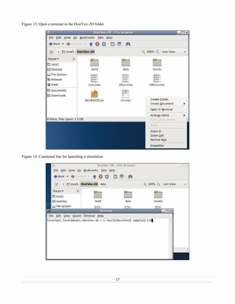
Figure 13: Open a terminal in the DosiVox-2D folder
Figure 14: Command line for launching a simulation
17
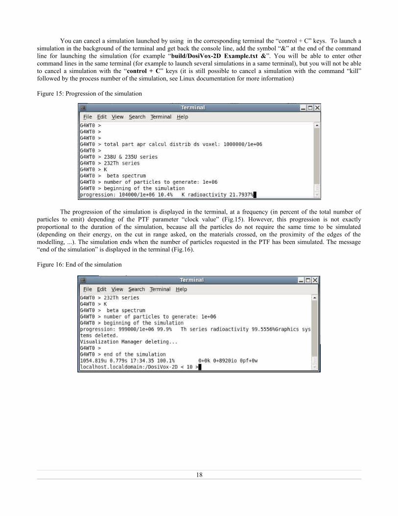
You can cancel a simulation launched by using in the corresponding terminal the “control + C” keys. To launch asimulation in the background of the terminal and get back the console line, add the symbol “&” at the end of the commandline for launching the simulation (for example “build/DosiVox-2D Example.txt &”. You will be able to enter othercommand lines in the same terminal (for example to launch several simulations in a same terminal), but you will not be ableto cancel a simulation with the “control + C” keys (it is still possible to cancel a simulation with the command “kill”followed by the process number of the simulation, see Linux documentation for more information)
Figure 15: Progression of the simulation
The progression of the simulation is displayed in the terminal, at a frequency (in percent of the total number ofparticles to emit) depending of the PTF parameter “clock value” (Fig.15). However, this progression is not exactlyproportional to the duration of the simulation, because all the particles do not require the same time to be simulated(depending on their energy, on the cut in range asked, on the materials crossed, on the proximity of the edges of themodelling, ...). The simulation ends when the number of particles requested in the PTF has been simulated. The message“end of the simulation” is displayed in the terminal (Fig.16).
Figure 16: End of the simulation
18
5 – Result processingThe Result Text Files (RTF)
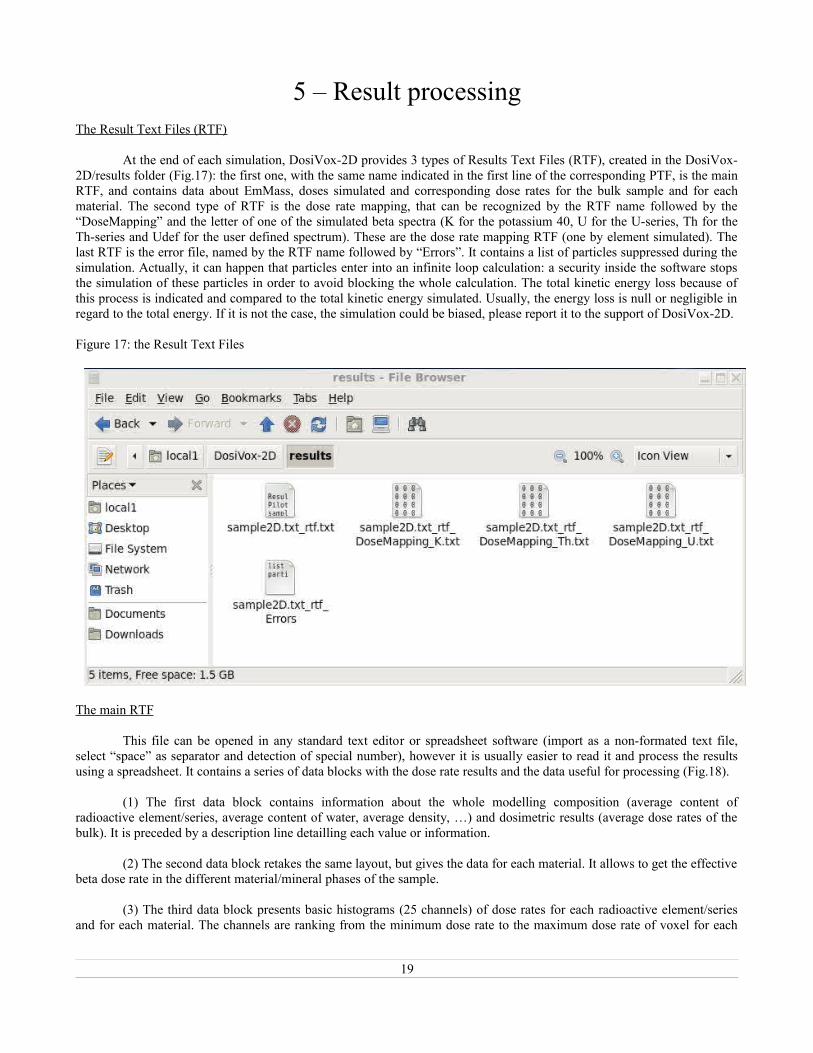
At the end of each simulation, DosiVox-2D provides 3 types of Results Text Files (RTF), created in the DosiVox-2D/results folder (Fig.17): the first one, with the same name indicated in the first line of the corresponding PTF, is the mainRTF, and contains data about EmMass, doses simulated and corresponding dose rates for the bulk sample and for eachmaterial. The second type of RTF is the dose rate mapping, that can be recognized by the RTF name followed by the“DoseMapping” and the letter of one of the simulated beta spectra (K for the potassium 40, U for the U-series, Th for theTh-series and Udef for the user defined spectrum). These are the dose rate mapping RTF (one by element simulated). Thelast RTF is the error file, named by the RTF name followed by “Errors”. It contains a list of particles suppressed during thesimulation. Actually, it can happen that particles enter into an infinite loop calculation: a security inside the software stopsthe simulation of these particles in order to avoid blocking the whole calculation. The total kinetic energy loss because ofthis process is indicated and compared to the total kinetic energy simulated. Usually, the energy loss is null or negligible inregard to the total energy. If it is not the case, the simulation could be biased, please report it to the support of DosiVox-2D.
Figure 17: the Result Text Files
The main RTF
This file can be opened in any standard text editor or spreadsheet software (import as a non-formated text file,select “space” as separator and detection of special number), however it is usually easier to read it and process the resultsusing a spreadsheet. It contains a series of data blocks with the dose rate results and the data useful for processing (Fig.18).
(1) The first data block contains information about the whole modelling composition (average content ofradioactive element/series, average content of water, average density, …) and dosimetric results (average dose rates of thebulk). It is preceded by a description line detailling each value or information.
(2) The second data block retakes the same layout, but gives the data for each material. It allows to get the effectivebeta dose rate in the different material/mineral phases of the sample.
(3) The third data block presents basic histograms (25 channels) of dose rates for each radioactive element/seriesand for each material. The channels are ranking from the minimum dose rate to the maximum dose rate of voxel for each
19
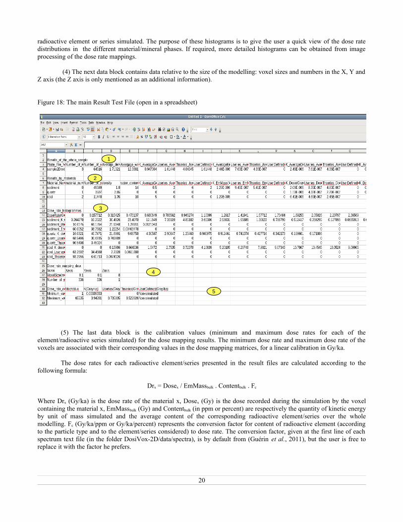
radioactive element or series simulated. The purpose of these histograms is to give the user a quick view of the dose ratedistributions in the different material/mineral phases. If required, more detailed histograms can be obtained from imageprocessing of the dose rate mappings.
(4) The next data block contains data relative to the size of the modelling: voxel sizes and numbers in the X, Y andZ axis (the Z axis is only mentioned as an additional information).
Figure 18: The main Result Test File (open in a spreadsheet)
(5) The last data block is the calibration values (minimum and maximum dose rates for each of theelement/radioactive series simulated) for the dose mapping results. The minimum dose rate and maximum dose rate of thevoxels are associated with their corresponding values in the dose mapping matrices, for a linear calibration in Gy/ka.
The dose rates for each radioactive element/series presented in the result files are calculated according to thefollowing formula:
Drx = Dosex / EmMassbulk . Contentbulk . Fc
Where Drx (Gy/ka) is the dose rate of the material x, Dosex (Gy) is the dose recorded during the simulation by the voxelcontaining the material x, EmMassbulk (Gy) and Contentbulk (in ppm or percent) are respectively the quantity of kinetic energyby unit of mass simulated and the average content of the corresponding radioactive element/series over the wholemodelling. Fc (Gy/ka/ppm or Gy/ka/percent) represents the conversion factor for content of radioactive element (accordingto the particle type and to the element/series considered) to dose rate. The conversion factor, given at the first line of eachspectrum text file (in the folder DosiVox-2D/data/spectra), is by default from (Guérin et al., 2011), but the user is free toreplace it with the factor he prefers.
20
1
2
3
4
5

If the objects of interest are grains inside one of the material/mineral phases of the modelling, the dose ratecalculated for this phase can be considered as the dose rate coming from the environment containing the grains. Therefore, itis possible to calculate the dose rate in grains just by applying an attenuation factor for moisture (Zimmerman, 1971, Nathanand Mauz, 2008) and grain size (Aitken, 1985, Guérin et al., 2012). However, users have to consider that these tabulatedfactors were calculated for environments with poor and scattered grains fraction, surrounded by a homogeneous fine matrix.Published data show that they may not be suitable for materials presenting a significant coarse fraction of grains (Guérinand Mercier, 2012) or if the material contains radioactive hotspots that are not represented in the modelling (Guérin et al.,2012). However two particular cases can be highlighted: if the grain size is very small compared to the particle range (as itis for fine grains under 10µm and beta particles) or if the grain fraction totally fills the material (for example if the materialis composed of an agglomerate of grains of the same mineral), then there is no need to apply attenuation factor for grain sizeas the dose rate received by the grains will be the same than in the material/mineral phase. However it is still necessary toremove the part of the dose rate absorbed by the moisture.
The dose rate mappings
The dose mapping results are text matrix with the same layout than the 2D image used for the model creation. Eachvalue of the matrix represents the dose rate recorded by the voxel at this location. There is one mapping file by elementsimulated, plus a total dose rate mapping file. These files can be opened into a spreadsheet, or read as a 16 bit text image(with ImageJ for instance). The dose rate of each file is distributed from the values 1 (corresponding to the minimum doserate of a voxel) to 65535 (maximum value of a 16bit image, corresponding here to the maximum dose rate of a voxel). Thevalue “0” corresponds to the EEZ (Edge Effect Zone) when it is excluded from the results or to the materials not representedif you chose the dose mapping option for one material only (see part 3). To calibrate the dose mapping files in Gy/ka (linearcalibration), use the values of the last data block of the main result file.
In addition to the visualization of the dose rates, the dose mapping files, once calibrated, allow to use imageprocessing for investigating dose rates distribution. It is therefore possible to obtain histograms of dose rates distribution fordifferent areas of the modelling. You can also isolate the dose rates in a material/mineral phase using the original segmentedimage of the sample slice by creating ROI (Region of Interest) or a binary mask of the material/mineral phase, and applyingit to the dose mapping ( https://imagej.nih.gov/ij/ ). It is also possible (by using for example the mathematical process ofImageJ or a simple spreadsheet) to apply attenuation factors for moisture and grain size (when required) to the dosemapping or to a ROI, and also to add/average different dose mappings together (once the attenuation factor are applied forexample, or if several simulations were carried on with the same modelling). Notice that if you use the ImageJ software, it isrecommended, once the dose mappings have been calibrated as 16bit images, to convert them in 32bit images. More processoptions will be available, and the results of the mathematical processes will be more accurate.
21
6 – ReferencesAitken, M.J., 1985. Thermoluminescence Dating. Academic Press, London, 378 p. https://doi.org/10.1002/gea.3340020110
Agostinelli et. al., 2003. Geant4 - a simulation toolkit. Nuclear instruments & methods in physics research, Section A, 506, 250-303. https://doi.org/10.1016/S0168-9002(03)01368-8
Allison , J., et. al., 2006. Geant4 developments and applications. IEEE Transactions on Nuclear Science 53, 270-278, https://doi.org/10.1109/TNS.2006.869826
Allison, J., et al., 2016. Recent developments in Geant4 Nuclear Instruments and Methods in Physics Research Section A: Accelerators, Spectrometers, Detectors and Associated Equipment 835, 186-225. https://doi.org/10.1016/j.nima.2016.06.125
Fang, F., Martin, L., Williams, I., Brink, F., Mercier, N., Grün, R., 2018. 2D modelling: A Monte Carlo approach for assessing heterogeneous beta dose rates in luminescence and ESR dating: Paper ΙΙ, application to igneous. Quaternary Geochronology, in press. https://doi.org/10.1016/j.quageo.2018.07.005
Guérin, G., Mercier, N., Adamiec, G., 2011. Dose-rate conversion factors: update. Ancient TL 29, 5-8. http://ancienttl.org/ATL_29-1_2011/ATL_29-1_Guerin_p5-8.pdf
Guérin, G., Mercier, N., 2012. Preliminary insight into dose deposition processes in sedimentary media on a scale of single grains: Monte Carlo modelling of the effect of water on the gamma dose rate. Radiation Measurements 47, 541 – 547. https://doi.org/10.1016/j.radmeas.2012.05.004
Guérin, G. , Mercier, N., Nathan, R. , Adamiec, G. and Lefrais, Y., 2012. On the use of the infinite matrix assumption and associated concepts: a critical review. Radiation Measurements 47, 778 – 785. https://doi.org/10.1016/j.radmeas.2012.04.004
Incerti, S., Baldacchino, G., Bernal, M., Capra, R., Champion, C., Francis, Z., Guatelli, S., Gueye, P., Mantero, A., Mascialino, B., Moretto, P., Nieminen, P., Rosenfeld, A., Villagrasa, C. & Zacharatou, C. (2010). THE Geant4-DNA
project. International Journal of Modeling, Simulation, and Scientific Computing, 1 (2), 157-178. http://dx.doi.org/10.1142/S1793962310000122
Kinsey, R.R.; Dunford, C.L.; Tuli, J.K. & Burrows, T.W., 1996. The NUDAT/PCNUDAT Program for Nuclear Data. 9th International Symposium of Capture Gamma-Ray Spectroscopy and Related Topics, Budapest, Hungary, October 1996. Data extracted from the NUDAT database, version nov 2009 and janv 2013,[https://www.nndc.bnl.gov/nudat2/reCenter.jsp?z=50&n=63]
Kramida, A., Ralchenko, Yu., Reader, J. and NIST ASD Team, 2018. NIST Atomic Spectra Database (version 5.0.0), https://physics.nist.gov/asd [Nov 2012]. National Institute of Standards and Technology, Gaithersburg, MD. https://doi.org/10.18434/T4W30F
Martin, L., 2015. Caractérisation et modélisation d'objets archéologiques en vue de leur datation par des méthodes paléo-dosimétriques : simulation des paramètres dosimétriques sous Geant4. Thèse de doctorat en Physique des archéomatériaux, Bordeaux, université Bordeaux-Montaigne, 304p. http://www.theses.fr/2015BOR30055
Martin, L., Incerti, S., Mercier, N., 2015a. DosiVox : a Geant 4-based software for dosimetry simulations relevant to luminescence and ESR dating techniques. Ancient TL 33 n°1, 1-10. http://ancienttl.org/ATL_33-1_2015/ATL_33-1_Martin_p1-10.pdf
Martin, L., Mercier, N., Incerti, S., Lefrais, Y., Pecheyran, C., Guerin, G., Jarry, M., Bruxelles, L., Bon, F., Pallier C., 2015b. Dosimetric study of sediments at the Beta dose rate scale : characterization and modelization with the DosiVox software. Radiation Measurement 81, 134-141. https://doi.org/10.1016/j.radmeas.2015.02.008
22
Martin, L., Incerti, S., Mercier, N., 2015c. Comparison of DosiVox simulation results with tabulated data and standard calculations. Ancient TL 33 n°2, 1-9. http://ancienttl.org/ATL_33-2_2015/ATL_33-2_Martin_p1-9.pdf
Martin, L., Fang, F., Mercier, N., Incerti, S., Grün, R., Lefrais, Y., 2018. 2D modelling: A Monte Carlo approach for assessing heterogeneous beta dose rates in luminescence and ESR dating: Paper Ι, theory and verification. Quaternary Geochronology, in press. https://doi.org/10.1016/j.quageo.2018.07.004
Nathan, R.P. , Mauz, B., 2008. On the dose-rate estimate of carbonate-rich sediments for trapped charge dating. Radiation Measurements 43, 14-25. https://doi.org/10.1016/j.radmeas.2007.12.012
Rasband, W.S., 1997 – 2012. ImageJ, U.S. National Institutes of Health, Bethesda, Maryland, USA,imagej.nih.gov/ij/
Underwood, E.E., 1970. Quantitative Stereology. Addison-Wesley, 274p. ISBN-13: 978-0201076509
Zimmerman, D.W., 1971. Thermoluminescent dating using fine grains from pottery. Archaeometry 10, 26–28. https://doi.org/10.1111/j.1475-4754.1971.tb00028.x
For technical support, please contact :
Loïc MARTIN: [email protected] MERCIER: [email protected]
DosiVox-2D and corresponding documentation are available at http://www.iramat-crp2a.cnrs.fr/spip/spip.php?article144.
23