User Manual for the Corporate Vulnerability Utility

By Robin Brooks and Kenichi Ueda1

April 6, 2005 A. Introduction The Corporate Vulnerability Utility (CVU) provides indicators for surveillance of the corporate sector in 53 countries. These indicators are based on underlying data from the annual reports of publicly traded companies and capture four types of risk: • balance sheet risk: indicators that capture risk associated with excessive leverage, poor

liquidity, low profitability, and high valuation; • international business cycle risk: indicators that measure the exposure of the corporate

sector to shocks from abroad though foreign sales, assets, and income; • external financing risk: indicators that measure the sensitivity of investment to tighter

financing conditions during a credit crunch or stock market crash; • default risk: indicators that summarize many dimensions of risk into a single statistic, a

forward-looking probability of default. The CVU provides easy access to these indicators via an interactive window in Excel. This window allows users to download annual indicators from 1990 at the country, region and industry levels. The CVU generates these indicators in the following steps: 1. Identifying indicators: the CVU synthesizes information from inside and outside the

Fund to identify the appropriate set of vulnerability indicators. 2. Downloading data: the CVU downloads required balance sheet, cash flow and income

statement items from Worldscope. Separately, it also downloads stock price and market capitalization data from Datastream.

1 We are grateful to seminar participants in APD, EUR, MFD, and WHD for many helpful comments. Special thanks go to Albert Jaeger, Simon Johnson, Guy Meredith, Jonathan Ostry, Eswar Prasad and Raghu Rajan for continued support and feedback. Finally, we thank Kellett Hannah, Qin Liu, and Farhad Nourbakhsh for superb technical support, and Eisuke Okada, Junko Sekine, and Wellian Wiranto for outstanding research assistance.

- 2 -

3. Cleaning data: the CVU ensures that every firm is represented in the data only once, in the country of its primary listing. It checks that firms that cease operations exit the data, and drops outliers.

4. Assessing coverage: the CVU constructs indicators on whether the data provide good coverage of publicly traded firms in each country. It also constructs an indicator to pick up how important publicly traded firms are relative to the overall economy.

5. Calculating indicators: the CVU calculates firm-level vulnerability indicators, ranging

from standard accounting ratios to option pricing-based default probabilities. 6. Aggregating indicators: the CVU provides simple and market capitalization-weighted

averages of firm-level indicators for countries, regions and industries. It also displays the representative observation at the bottom quartile, at the median, and at the top quartile.

7. Updating data: the CVU updates the set of vulnerability indicators every quarter, so that

they can be used for ongoing surveillance. The CVU aims to make ongoing surveillance of the corporate sector easier. It does this in a number of ways:

The CVU frees users from the time-consuming task of constructing vulnerability indicators. By providing ready-made indicators, the CVU allows users to focus on surveillance.

The CVU is easy to use. Its Excel-based interactive window allows users to quickly

access vulnerability indicators, and this user manual reviews these indicators and their strengths and weaknesses.

The CVU provides a common platform for corporate surveillance across countries.

It centralizes the downloading, cleaning and aggregating of firm-level data, providing a consistent framework for corporate surveillance across departments.

The CVU automatically updates indicators every quarter. This feature is critical for

ongoing surveillance. Many economists currently download Worldscope data on a one-off basis, which means that corporate surveillance lacks continuity.

The CVU systematically assesses the quality of coverage for each country. It does

this by comparing coverage of firms for each country to that in the S&P Global Stock Markets Factbook, a widely-used alternate data source.

The CVU constructs indicators in a transparent way. The CVU spells out exactly how

indicators are constructed and allows users to modify them. For example, some indicators are weighted averages of underlying accounting ratios. The CVU allows users to change the weights, which are often based on estimates for US data and may not carry over to other countries, especially emerging markets.

- 3 -

The CVU provides an improved measure of systemic risk to the corporate sector as a whole. The pooled Black-Scholes-Merton default probability nets out idiosyncratic risk among companies, isolating systemic risk to the overall corporate sector.

The underlying data have several limitations. The CVU addresses these in several ways: • Worldscope covers only publicly traded firms. The CVU systematically documents the

quality of coverage, by comparing coverage to the S&P Global Stock Markets Factbook, both in terms of number of companies in each country and in terms of market cap. It also compares the capitalization of the stock market to GDP, to assess whether many firms are unlisted, in which case the stock market is a poor measure of the full corporate sector.

• Worldscope does not break out the currency composition of debt. The CVU includes

option pricing-based default probabilities, which should incorporate all publicly available information through stock prices and their volatility. Hence, these default probabilities should capture risks from foreign currency debt exposure, and possible natural hedging through foreign sales. These indicators are also forward-looking, while balance sheet data on currency composition are not.

• There is a lag in the updating of Worldscope data, due to the fact that reporting dates

for individual companies are distributed throughout the year. This means that the CVU is ill-suited for high frequency corporate surveillance and is better suited for monitoring broad trends in corporate balance sheets.

We suggest using the CVU in the following steps. Before looking at the vulnerability indicators themselves, it is critical to get a sense of the quality of the underlying data. This means studying the importance of the stock market in relation to the overall economy, and getting a feel for how coverage changes over time. Next, we suggest getting a sense for the overall trends in corporate vulnerability, using the default risk indicators. These indicators have two advantages. First, they bundle various dimensions of risk into one statistic, allowing a rise in leverage to be offset by a rise in liquidity, for example. Second, they are forward-looking. Finally, we suggest taking a disaggregated look at corporate vulnerability, using accounting ratios, to get a sense of what factors are driving changes in overall corporate vulnerability. For cross-country comparisons, we suggest using market capitalization-weighted averages. These weighted averages have two advantages. First, they collapse the data toward the largest, economically most important firms, thereby focusing on systemic corporate risk. Second, they control for differences across countries in depth of coverage. For example, the CVU has data on 7,587 firms in the US in 2003. In contrast, Chile has 168 firms. Comparing the medians of both countries would be misleading, because the representative firm in the US is small, while it is relatively larger for Chile. The medians and upper and lower quartiles are more useful for looking at time-series within countries, or for comparisons across markets with similar coverage.

- 4 -

The remainder of this paper is structured as follows. Section B provides a summary of country, region and industry coverage. Section C lists the indicators, places them in the context of the recent literature, and explains their strengths and weaknesses. Section D reviews how the CVU cleans and aggregates firm-level data. Section E looks at how good data coverage is for individual countries. Section F gives a case study for using the CVU. Appendix I provides data codes for all Worldscope and Datastream items and provides tables on cut-offs for outliers and the number of firms in Datastream indices. Appendix II provides summary tables for all indicators, by country and year, in addition to the number of firms underlying each indicator, again by country and year. Because of its length, Appendix II is not included in this document, but can be downloaded separately from the “Data Summary” link on the CVU website. B. Coverage This section gives an overview of country, region and industry coverage. The CVU covers 53 countries. Following the Morgan Stanley Capital International (MSCI) indices, these countries are divided into 7 regions: Developed Americas (DAM), Emerging Americas (EAM), Developed Asia (DAS), Emerging Asia (EAS), Developed Europe (DEU), Emerging Europe (EEU), and the Middle-East and Africa (MEA). The CVU also provides indicators for the Euro Zone, which is included as a separate entry in the Developed Europe region. At the regional level, including the Euro Zone, indicators are calculated by pooling firm-level data for all countries in a given region. For more information on the MSCI classification, see http://www.msci.com/equity/coverage_matrix.pdf. Table 1 lists the countries and gives their region affiliations. Each company is assigned to one of 10 FTSE industry groups: Resources, Basic Industries, General Industrials, Cyclical Consumer Goods, Non-Cyclical Consumer Goods, Cyclical Services, Non-Cyclical Services, Utilities, Financials, Information Technology. In addition, the CVU provides indicators for the non-financial corporate sector, which aggregates data for firms in all industries except the financial sector. For more information on these groups, see http://www.datastream.com/product/investor/index.htm.

- 5 -

Table 1. Country and Region Coverage Developed Americas (DAM) Developed Asia (DAS) Developed Europe (DEU) Middle-East and Africa (MEA)

CANADA AUSTRALIA AUSTRIA EGYPTUSA HONG KONG BELGIUM ISRAEL

JAPAN DENMARK MOROCCONEW ZEALAND FINLAND PAKISTAN

SINGAPORE FRANCE SOUTH AFRICAGERMANY ZIMBABWE

GREECE IRELAND

ITALY LUXEMBOURG

NETHERLANDS NORWAY

PORTUGAL SPAIN

SWEDEN SWITZERLAND

UNITED KINGDOMEURO ZONE

Emerging Americas (EAM) Emerging Asia (EAS) Emerging Europe (EEU)ARGENTINA CHINA CZECH REPUBLIC

BRAZIL INDIA HUNGARYCHILE INDONESIA POLAND

COLOMBIA KOREA (SOUTH) RUSSIAN FEDERATIONMEXICO MALAYSIA SLOVAK REPUBLIC

PERU PHILIPPINES SLOVENIAVENEZUELA SRI LANKA TURKEY

TAIWANTHAILAND

C. Indicators This section lists the indicators provided by the CVU, defines their construction and explains their intuition. The indicators fall into five broad groups: (i) measures of data coverage; (ii) accounting ratios; (iii) measures of international exposure; (iv) measures of dependence on external financing; and (v) measures of default risk. Table 2 gives an overview of the various indicators in each category.

Table 2. Panel A. Accounting Ratios Leverage Liquidity Profitability Valuation

Debt-to-Equity (in %) Quick Ratio Return on Assets (in %) Price-to-Earnings RatioDebt-to-Assets (in %) Current Ratio Return on Equity (in %) Market-to-Book RatioDebt-to-Sales (in %) Cashflow to Sales in % Tobin's Q

Debt-to-Cashflow (in %) Interest Coverage RatioShort-Term Debt in % Total Debt Estimated Avg. Interest Rate in %Total Liabilities in % Total Assets

Current Liabilities in % Total LiabilitiesCurrent Assets in % Total Assets

- 6 -

Table 2. Panel B. Other Indicators Data Description External Dependence External Financing Default RiskNumber of Firms Foreign Sales in % Total Sales Kaplan & Zingales (1997) Index Z-Score and Z-Probability

Market Cap in Millions of USD Foreign Assets in % Total Assets Rajan & Zingales (1998) Index O-Score and O-ProbabilityNumber of Firms in % of S&P Benchmark Foreign Income in % Total Income Black-Scholes-Merton Default Probability

Market Cap in % of S&P BenchmarkMarket Cap in % of GDP

Future versions of the CVU aim to incorporate additional indicators. In particular, recent academic work has found measures of corporate governance and ownership structure to be important determinants of performance. Mitton (2002) finds that firm-level differences in variables related to corporate governance have a strong impact on firm performance during the East Asian financial crisis in 1997 – 1998. Joh (2003) finds that ownership structure and conflicts of interest among shareholders under a poor corporate governance system affected firm performance in Korea in the years before the East Asian financial crisis.2 More generally, the CVU aims to continually expand the measures of risk. Additional indicators could measure currency composition of corporate debt, economic activity, etc. C.1 Measures of Data Coverage The CVU provides statistics by country and region that describe data coverage. These statistics address two main concerns: (i) coverage of listed firms may vary across countries and over time; and (ii) the listed universe of firms may not provide a good representation of the corporate sector, if a significant number of corporations are unlisted. To address the first concern, the CVU compares data coverage in terms of number of firms and market caps to the S&P Global Stock Markets Factbook. To address the second, the CVU provides the ratio of total market capitalization to GDP. The full set of data coverage indicators is:

• number of firms • market capitalization in millions of USD • number of firms in percent of S&P Global Stock Markets Factbook • market capitalization in percent of S&P Global Stock Markets Factbook • market capitalization in percent of GDP

C.2 Accounting Ratios Analysis of the corporate sector should cover: (i) leverage; (ii) liquidity; (iii) profitability; and (iv) valuation. This section discusses each of these areas in turn. 2 Todd Mitton. 2002. “A Cross-Firm Analysis of the Impact of Corporate Governance on the East Asian Financial Crisis.” Journal of Financial Economics 64: 215 – 241. Sung Wook Joh. 2003. “Corporate Governance and Firm Profitability: Evidence from Korea before the Economic Crisis.” Journal of Financial Economics 68: 287 – 322.

- 7 -

C.2.1 Leverage Leverage is a key measure of corporate sector vulnerability. Highly leveraged corporate sectors have little equity relative to assets, so they are at higher risk of insolvency in response to shocks that reduce the value of assets and hence equity. Actual or threatened insolvency will lead to reduced access to finance and/or bankruptcy. The CVU reports all measures of leverage in percent. The leverage indicators are as follows:

• debt-to-equity • debt-to-assets • debt-to-sales • debt-to-cashflow • short-term to total debt • total liabilities to total assets • current liabilities to total liabilities • current assets to total assets

Leverage indicators are subject to distortions and must be used carefully. There is often a discrepancy between book and market value of debt, because accounting measures of debt do not adjust for interest rate risk. In addition, debt-to-equity and debt-to-assets are subject to potential measurement error in the book value of equity or assets. Underlying weakness may be masked during a stock market or real estate bubble, for example, when assets (and hence equity) may be overvalued. As a result, debt-to-sales or debt-to-cashflow may be better indicators. The ratio of short-term to total debt examines the maturity structure of debt. The numerator of this indicator captures debt payable within one year including the current portion of long-term debt. When companies become financially distressed, this ratio tends to rise as lenders prefer shorter-term exposures. Total liabilities is the most comprehensive measure of firms’ obligations. This measure includes current liabilities, long-term debt, pension benefits, and unrealized losses on marketable securities. The ratio of total liabilities to total assets is thus the most comprehensive measure of leverage. C.2.2 Liquidity Liquidity is a buffer against shocks to financing and cashflow, and declining liquidity ratios may be an indication of financial difficulties. Firms typically first respond to shocks by drawing down their liquid assets and allowing accounts payable to rise, so falling liquidity ratios can be a signal of financial distress. A less liquid company is more likely to become delinquent on loans if cashflow turns negative or new financing is limited. The CVU reports five liquidity indicators:

• current ratio • quick ratio • cashflow to sales • interest coverage ratio

- 8 -

• estimated average interest rate The current ratio is the ratio of current assets to current liabilities. It measures the ability of a firm to pay its short-term obligations with assets that can easily and quickly be converted into cash. Current assets refer to cash and other assets that can be liquidated and converted to cash within one year, e.g. cash, marketable securities, accounts receivable, and inventory. Current liabilities are obligations that require cash payment within one year (e.g. short-term debt, accounts payable, wages, taxes, etc). The quick ratio is a stricter measure of liquidity than the current ratio, because it nets out inventories from current assets. This is because inventories are considered the least liquid of current assets. The quick ratio therefore compares cash, cash equivalents and net receivables to current liabilities. High levels of leverage may be more sustainable if profits are high relative to interest payments, as measured by the interest coverage ratio (ICR). This ratio compares earnings before interest and taxes (EBIT) to interest payments falling due. When this ratio is less than one, it can mean that a firm is in arrears on its interest payments. However, other indicators of liquidity are needed to get a more complete picture of financial distress, because ICRs do not account for all resources that a company has available to meet its debt service payments. During a recession or period of restructuring, companies may show a sharp decline in ICRs, but liquid assets may allow them to remain current on their payments. This ratio can also be constructed using EBITDA, which may be a better measure of cashflow available for interest obligations, since depreciation is a non-cash expense. Finally, because profitability is a key input for the ICR, the CVU also provides an alternate measure of liquidity relative to sales: cashflow to sales. The estimated average interest rate is calculated by dividing interest expense on debt by total debt. This interest rate will be higher for firms that are more financially distressed. C.2.3 Profitability Profits are a sign of financial strength that can shape the response of creditors to shocks. Large one-time losses are manageable if firms generate sufficient profits. Creditors are less likely to withdraw credit for more profitable firms. The CVU provides two measures of profitability, both of which are reported in percent:

• return on assets • return on equity

The return on assets (RA) is the ratio of net income to total assets and measures the efficiency with which a company uses its assets. Net income is the bottom line measure of total earnings after adjustments for operating costs, depreciation, interest, taxes, and other expenses. RA can be expressed as the product of profit margin (net income divided by

- 9 -

operating revenue) and asset turnover (operating revenue over total assets). Separating these components of RA may shed light on whether firms are raising RA via higher profit margins or greater turnover of their assets. For example, service companies like luxury goods stores typically have high margins but low turnover, while retail firms such as discount warehouse have low margins but high turnover. Persistently low or declining RA at the sectoral level could be an indication of excess capacity (reduced margins) or low productivity. The return on equity (RE) is the ratio of net income to shareholders’ equity and measures the return to shareholders on their investment. It may be useful to break down RE into the return on assets (net income/total assets) and the equity multiplier (total assets/equity). Firms may boost their RE by raising their return on assets or by taking on more leverage. C.2.4 Valuation These indicators combine accounting and stock market data to provide a measure of the stock market valuation of a company relative to its earnings and growth potential. Standard finance textbooks, such as Corporate Finance by Ross and others (2002), provide detailed descriptions of these measures.3 The CVU has three valuation measures:

• price-to-earnings ratio • market-to-book ratio • Tobin’s Q

The P/E ratio is a common measure of the esteem in which a firm is held by investors. This ratio divides the stock price of a company by its earnings per share. If the dividends of a company are expected to grow at a steady rate, the current stock price can be written as P = Div/(r – g) where Div measures expected dividends next year, r is the return that investors require from similar investments next year, and g is the expected rate of dividend growth. The P/E ratio can thus be written as:

grEDiv

EP

−×=

1

A high P/E ratio may mean (i) investors expect high dividend growth (g); (ii) the stock has low risk and investors are content with a low prospective return (r); or (iii) a company is expected to achieve average growth while paying out a high proportion of earnings. The market-to-book ratio is the ratio of stock price to book value per share. Book value per share is stockholders’ book equity (net worth) divided by number of shares outstanding.

3Stephen A. Ross, Randolph W. Westerfield, Jeffrey Jaffe. 2002. “Corporate Finance.”

- 10 -

Book equity equals common stock plus retained earnings—the net amount a firm received from stockholders or reinvested on their behalf. A ratio of 1.25, for example, means that a firm is worth 25 percent more than past and present shareholders have put into the company. Investment managers classify firms with high book-to-market ratios as value stocks, which are seen as having higher risk of financial distress than growth stocks (low book-to-market ratios). Consistent with this notion, Fama and French (1998) find that value stocks tend to have higher returns than growth stocks in equity markets around the world.4 Tobin’s Q is defined as the ratio of the market value of a company’s debt and equity to the current replacement cost of assets. However, because the market value of debt and replacement cost of asset are hard to measure, the CVU approximates Q as market value of equity plus book value of debt, divided by book value of assets. James Tobin argued that firms have an incentive to invest when Q is greater than one (i.e. when capital equipment is worth more than it costs to replace), and that they will stop investing only when Q is equal to one (i.e. when the value of equipment falls to replacement cost). From an M&A perspective, if the market value of a company is smaller than its replacement cost of asset, an investor can profit from purchasing the company. Hence, in either case, Tobin’s Q should be one in equilibrium. In practice, however, this is not often the case, reflecting both imperfect markets and measurement error.5 If a firm faces financial constraints, Q can become higher than one. An example is a start-up company: while investors recognize growth potential and price the stock accordingly, the company cannot borrow sufficiently and operates with low total assets. Shrinking industries are an illustration of the opposite. Measurement error is associated with valuation of intangible assets. When intangible assets are not well recorded, Q can become higher than one, as is often the case with companies with strong brand images or patent protection. C.3 Measures of External Dependence This section presents three indicators that measure the exposure of the corporate sector to foreign shocks. These indicators are based on firm-level data on the importance of foreign operations for firms’ sales, assets and profitability. At the country level, these measures give an indication of the sensitivity of the corporate sector to shocks from abroad. At the industry level, they help distinguish between industries that are more versus less global and therefore provide information on how industrial structure affects the sensitivity of countries to foreign shocks. The three indicators, which are measured in percent, are: 4 Eugene F. Fama and Kenneth R. French. December 1998. “Value versus Growth: The International Experience.” Journal of Finance 53: 1975 - 1999.

5 For example, see discussions in Abdul Abiad, Nienke Oomes, and Kenichi Ueda, 2004, “The Quality Effect: Does Financial Liberalization Improve the Allocation of Capital?” IMF Working Paper WP/04/112.

- 11 -

• foreign sales to total sales • foreign assets to total assets • foreign income to total income

A limitation of the foreign sales and income data is that they reflect only sales and income generated by operations abroad (i.e., through foreign subsidiaries), and therefore omit sales and income associated with exports. These variables are therefore a lower bound on the international exposure of the corporate sector. Furthermore, unlike the accounting ratios above, foreign sales, assets and income are not standard reporting items in firms’ annual reports, which means that they may be subject to selection bias. For example, companies may report data only in favorable years. More generally, the quality of these variables is less good than for other Worldscope data. However, Brooks and Del Negro (2003) find that firms with a high foreign component to sales, assets or income also tend to have stock returns that comove more with global shocks. This is evidence that the indicators correctly identify firms with more international operations.6 Regional aggregates are calculated by pooling firm-level data within a given region, including for the Euro Zone. Because this does not net out international sales within a region, the regional international sales ratios are overstated. The same goes for the regional international asset and international income ratios. C.4 Measures of Dependence on External Financing This section presents two measures that quantify the extent to which companies depend on external sources of funds to finance investment. In the medium-term, the importance of external financing is related to financial depth and structure of a country.7 In the short-term, a rise in dependence on external financing may be a leading indicator for higher growth, if higher capacity utilization rates are spurring companies to invest more. At the same time, however, it can also be a risk factor, as it raises the sensitivity of a country to an unexpected “credit crunch.” A collapse in business investment in the event of a credit crunch can have larger adverse effects on economic activity. The CVU features two measures of dependence on external financing: (i) the Rajan and Zingales (1998) index of dependence on external financing; and (ii) the Kaplan and Zingales (1997) index of financial constraints. In perfect capital markets a firm’s investment decisions are independent of its financial condition. But if internal and external capital are not perfect substitutes—issuing debt and equity is costly because of transaction costs and asymmetric information. Fazzari, Hubbard 6 Robin Brooks and Marco Del Negro, forthcoming in 2005, “Firm-Level Evidence on International Stock Market Comovement,” Review of Finance.

7 Raghuram Rajan and Luigi Zingales. 1998. “Financial Dependence and Growth.” American Economic Review 88(3): 559 – 586.

- 12 -

and Petersen (1988) argue that firms’ internal cash flow may affect investment spending because of a “financing hierarchy,” whereby internal funds have a cost advantage over new debt or equity. Under these conditions, measures of dependence on external financing can be related to investment behavior and thus economic activity.8 C.4.1 The Rajan and Zingales (1998) Index This index measures dependence on external finance as a firm’s capital expenditures minus cash flow from operations divided by capital expenditures. The CVU presents this variable in percent—meaning it shows the percentage of total capital expenditures that are externally financed.9 Cashflow from operations is the sum of cashflow from operations, plus decreases in inventories, decreases in receivables, and increases in payables. This definition includes changes in the non-financial components of net working capital as part of funds from operations. In certain businesses these represent major sources (or uses) of funds that help a firm avoid (or force it to tap) external sources of funds.

CE - (CF + DF + DR + IP)RZ = CE

Capital expenditures (CE) refer to funds used to acquire fixed assets other than those associated with acquisitions. Cashflow consists of two components: (i) income before extraordinary items and preferred and common dividends, but after taking into account the operating and non-operating income and expense, reserves, income taxes, minority interest and equity in earnings; and (ii) depreciation, depletion and amortization. Decrease in inventory (DF) is generated by taking the difference between last period’s total inventories with those from the current period. Decrease in receivables (DR) is the difference between last period’s total receivables with this periods receivables. Finally, increase in payables (IP) is the difference between last period’s accounts payable with those from this period. This variable tracks the increase in accounts payable. Users can use the components of this index to construct a US Dollar measure of the financing gap. This measure is simply: CE – (CF + DF + DR + IP), and is denominated in thousands of US Dollars. 8 Steven Fazzari, Glenn Hubbard and Bruce Petersen. 1988. “Financing Constraints and Investment.” Brookings Papers on Economic Activity 1.

9 To measure dependence on external financing, Rajan and Zingales (1998) use Compustat data for the 1980s. They sum each component of the RZ index over the 1980s, firm by firm, to smooth out annual fluctuations, and then construct the ratio of investment financed externally for each firm. Then they report the RZ index as the median within industries. The CVU reports an annual RZ index to capture fluctuation between investment and cashflow.

- 13 -

C.4.2 The Kaplan and Zingales (1997) Index A variety of models suggest that financial constraints are important determinants of real activity and asset prices, see Bernanke et al. (1996) for a review. According to these models, imperfect capital markets serve to magnify macroeconomic shocks. The Kaplan and Zingales (1997) index measures the degree to which firms are likely financially constrained, and is higher for firms more likely to be constrained. The CVU follows Lamont and others (2001) in constructing this index: -1.001909*[cashflow to capital] + 0.2826389*[Tobin's Q] + 3.139193*[debt to capital] - 39.3678*[dividends to capital] - 1.314759*[cash to capital]. These coefficients are based on regressions by Kaplan and Zingales (1997) using data for U.S. manufacturing firms with positive real sales growth over the period 1969 to 1984. After calculating the KZ index for every firm, Lamont et al. (2001) classify the top 33 percent of all firms ranked on the KZ index as constrained.10 An important caveat to the Kaplan and Zingales (1997) index is that its coefficients are based on US data. These coefficients may not carry over to other countries, where financial markets are less developed or institutions and regulatory frameworks differ. To address this, the CVU makes the input variables for the index available for download. This allows users to adapt the index by changing the coefficients on the input variables. C.5 Default Probabilities This section presents three indicators that measure the risk of default. Relative to simple accounting ratios, they have two main advantages: (i) they are forward-looking; and (ii) they combine various dimensions of risk into a single statistic, which gives the overall impact on vulnerability from potentially offsetting changes, such as a rise in leverage versus a rise in profitability, for example. Of course, it is still important to monitor movements in individual accounting ratios to get a sense of underlying vulnerabilities. There are two ways to calculate default probabilities: one is empirical and combines accounting ratios into a single statistic, while the other is model-based and combines accounting data with stock price information. Two widely-used models in the first category are the Altman (1968)11 Z-Score model and the

10 Owen Lamont, Christopher Polk and Jesus Saa-Requejo. 2001. “Financial Constraints and Stock Returns.” The Review of Financial Studies 14(2): 529 – 554. Steven Kaplan and Luigi Zingales. 1997. “Do Financing Constraints Explain Why Investment is Correlated with Cash Flow?” Quarterly Journal of Economics (112): 168 – 216. Ben Bernanke, Mark Gertler and Simon Gilchrist. 1996. “The Financial Accelerator and the Flight to Quality.” Review of Economics and Statistics 78: 1 – 15.

11 Edward I. Altman, “Financial Ratios, Discriminant Analysis and the Prediction of Corporate Bankruptcy”, The Journal of Finance, Vol. 23, No. 4 (Sep., 1968), 589-609.

- 14 -

Ohlson (1980)12 O-Score model. Both are based on regression models to explain historical default patterns. The model-based approach uses the Black-Scholes-Merton option pricing model to derive the market’s assessment of default risk. Because the Black-Scholes-Merton default probability uses stock prices and their volatility as inputs, this measure incorporates all publicly available information and is therefore more comprehensive than the empirical models. C.5.1 The Altman (1968) Z-Score Altman (1968) develops a measure of distress that combines five accounting ratios. Letting

iD denote a binary variable (1 for default and 0 otherwise), the Altman (1968) model is similar to a logit regression where 1 , ,i nix xL are the accounting ratios:

exp( ) ,1 exp( )

ii

i

yDy

=+

with 0 1 1 , , .i i n niy x xα α α= + + +L

Altman (1968) calls iy− the Z-Score (higher Z means lower y and lower default probability). The Z-Score therefore captures the probability of survival (one year ahead) and is defined as follows:

Working Capital Retained Earnings EBIT-Score 1.2 1.4 3.3Total Asset Total Asset Total Asset

Market Value of Equity Sales0.6 0.999 ,Total Liabilities Total Asset

Z = + +

+ +

where EBIT stands for earning before interest and taxes. The Z-Probability is calculated using the cumulative density function for the logistic distribution:

ii

i

exp( -Score )-Prob = .1 exp( -Score )

ZZZ

−+ −

One caveat to Altman’s (1968) Z-Score is that the coefficients were estimated a long time ago based on a relatively narrow sample of US data. How applicable are these coefficients for the US today, and how well do they carry over to other countries, where attitudes towards default and the legal environment are different? Because of these questions, the CVU reports

12 James A. Ohlson, “Financial Ratios and the Probabilistic Prediction of Bankruptcy”, Journal of Accounting Research, Vol. 18, No.1 (Spring, 1980), 109-131.

- 15 -

makes all input variables available for download to users, so that they can change the coefficients. Updated coefficients for the US are available in Hillegeist and others (2004).13 C.5.2 The Ohlson (1980) O-Score The Ohlson (1980) O-Score measures the one-year-ahead probability of default (higher O means higher y and therefore a higher default probability). The O-Score combines nine accounting ratios into a single statistic:

Total Liability Working Capital-Score= 1.32 0.41Size 6.03 1.43Total Asset Total Asset

Current Liabilities Net Income FFO0.08 2.37 1.83Current Asset Total Asset Total Liabilities

0.285 1.72 0.52 ,

O

F G H

− − + −

+ − −

+ − −

where Size is the natural log of total asset divided by the GDP deflator;14 FFO means pre-tax income plus depreciation and amortization; F is an indicator variable equal to one if cumulative net income over the previous tow years is negative, and zero otherwise; G is an indicator variable equal to one if owners’ equity is negative and zero otherwise; and H is the scaled change in net income (NI): 1 1( ) /( ).t t t tNI NI NI NI− −− + The O-Probability is defined as:

ii

i

exp( -Score )-Prob = .1 exp( -Score )

OOO+

The caveat for Altman’s (1968) Z-Score carries over to Ohlson’s (1980) O-Score, which is estimated for US data. The CVU reports all input variables separately, allowing users to change the coefficients. Updated coefficients are available in Hillegeist and others (2004). C.4.3 The Black-Scholes-Merton (BSM) Default Probability The BSM default probability is calculated based on a widely-used theoretical asset pricing model. The BSM model in the CVU follows Hillegeist and others (2004) and Vassalou and Xing (2004)15 who apply the BSM formula16 to assess the probability of 13 Stephen A. Hillegeist, Elizabeth K. Keating, Donald P. Cram, and Kyle G. Lundstedt, “Assessing the Probability of Bankruptcy,” Review of Accounting Studies, 9, 5-34, 2004.

14 The CVU uses 2000 as the base year of the GDP deflator for all the countries.

15 Maria Vassalou and Yuhang Xing, “Default Risk in Equity Returns,” The Journal of Finance, Vol. LIX, No. 2, April 2004.

- 16 -

default. BSM derive the market’s assessment of default risk for a company from its equity price, assuming that the market price reflects investors’ correct calculation of default risk.17

• The BSM default probabilities show the theoretical probability of default one-year-ahead. See the formulas and computational notes below for further details.

• Distance-to-default, an input into the default probability, shows how much the

asset value needs to fall one-year-ahead for a firm to default given its current balance sheet position. It is reported in terms of the number of standard deviations of asset returns. The higher this number, the lower the BSM probability of default.

The model may generate default probabilities that are biased, if markets are not arbitrage free—possible in emerging markets with thin trading—or if the distribution of asset returns is not approximately normal. However, Hillegeist and others (2004) show that the BSM model predicts defaults for US data much better than the Z- or O-Score models. Because the BSM probability is a non-linear measure, creating default probabilities at the country, region or industry levels is more complicated that for other measures. The CVU does two things. As for other indicators, it calculates country, region or industry averages based on firm-level BSM probabilities. However, these measures do not provide a good indication of systemic risk, because they do not net out firm-specific risk. For this reason, the CVU reports pooled BSM probabilities, which treat the corporate sector in a country, region or industry as a portfolio. Inputs such as stock prices and balance sheet items are added up across companies to create a synthetic company at the country, region, and industry levels. The BSM probability is then calculated for this synthetic company, which corresponds to a portfolio of stocks. De Nicolo (2004) shows that these pooled BSM probabilities incorporate imperfect correlation of firm-level default risk and allow for time-variation in this correlation. The pooled BSM is thus the most appropriate measure of systemic risk to the corporate sector.18 The pooled BSM probability differs from the market cap-weighted average of firm-level BSM probabilities. If firm-specific shocks predominate, and the industrial structure of 16 Fischer Black and Myron Scholes, “The Pricing of Options and Corporate Liabilities,” Journal of Political Economy, 7, 637-654, 1973; Robert Merton, “On the Pricing of Corporate Debt: The Risk Structure of Interest Rates,” Journal of Finance, 29, 449-470, 1974.

17 Commercially available Moody’s KMV model works essentially in the same way, though the exact formula behind Moodys KMV is proprietary and not disclosed fully.

18 Gianni De Nicolo, “US Large Complex Banking Groups: Business Strategies, Risks, and Surveillance Issues,” IMF Country Report 04/228.

- 17 -

a country is well diversified, then the pooled BSM probability will typically be lower than the market cap-weighted average. If, however, firm-specific shocks are drowned out by a large common shock, the BSM probability may exceed the market cap-weighted average, especially if the corporate sector is dominated by a few disproportionately large firms. Formulas and Computational Notes Instantaneous distance-to-default: For a firm to survive, its assets must exceed its debt. Hence, log(Asset) - log(Debt) is a natural measure for distance to default. For practical reasons, short-term debt plus half of long term debt plus interest payments (defined as B) is typically used as the default barrier. If the value of assets falls below this level, a firm is assumed to declare default. To make the distance to default comparable across individual firms, it is normalized by the standard deviation of the asset return ( Aσ ). Letting A stand for assets,

Instantaneous distance-to-default = log( ) log( ) .A

A Bσ−

Distance-to-default within one year: as in Black and Scholes (1973) and Merton (1974), the logarithm of a firm’s assets is assumed to follow the standard Brownian motion, and thus

Distance-to-default within one year =

2

log( ) log( )2

,

A

A

A BDtD

σµ

σ

⎛ ⎞− + −⎜ ⎟

⎝ ⎠=

where µ is the expected return.19 Because DtD is normally distributed with mean zero, we add 3 to the calculated DtD measure so that the reported DtD is always positive.20 Reported distance-to-default within one year = 3.DtD + For example, if the reported distance-to-default is 3, a firm has enough assets not to default as long as the asset return does not drop 3 standard deviation from its current level within one year.

19 Following Vassalou and Xing (2004) and Hillegeist and others (2004), we use last year’s annual capital gain of assets as the expected return. While the latter use ex dividend returns with 200 percent as the upper bound and the risk free rate as the lower bound, we use cum dividend returns without bounds as in Vassalou and Xing. A priori bounds may be reasonable for US data, but they do not seem appropriate for volatile emerging market economies. We find little difference between the two ways of defining the formula.

20 In normal distributions, 3 standard deviation left from the mean has cumulative density of 1 percent.

- 18 -

BSM default probability within one year: By construction, DtD follows a standard normal distribution. Hence, lettingΦ denote the standard cumulative normal distribution, the probability of default is calculated as follows: BSM default probability within one year = . . ( ).Def Prob DtD= Φ − For example, in case the reported distance to default is 3 as in previous example, it is 0 in unadjusted terms, and the default probability is (0) 0.5,Φ = or 50 percent. Data on the value of assets and on the standard deviation of asset returns are not observed and thus need to be estimated using the Black-Scholes-Merton formula. Specifically, given the observed price of equity and the observed standard deviation of equity returns, the value of assets and the volatility of asset returns can be solved for, as there are two unknowns in two equations.21 The first is the Black-Scholes-Merton pricing formula: ( ) ,r

AE A DtD Beσ −= Φ + − where E is price of equity and r is the risk free rate. The second is the optimal hedge equation: ( ),E A AE A DtDσ σ σ= Φ + where Eσ is the standard deviation of equity prices. The annualized weekly equity return is used to calculate Eσ for each firm in each year.22 D. Data Cleaning and Aggregation This section discusses the process of data cleaning and aggregation. It provides detailed explanations for how outliers are dropped from the underlying data, and reviews how the

21 These equations are highly non-linear and are solved iteratively by first the fixing standard deviation of asset returns to search over the asset value, and then fixing the asset value to search over standard deviation, until the squared error of approximation falls within 0.001 for each firm in each year. Hillegeist and others (2004) simultaneously solve two equations. This method sometimes fails to deliver the solution for our dataset. Vassalou and Xing (2004) calculate asset values (the first equation) daily and obtain the sample variance of assets without using the second equation. Although it may be a superior method, this computation requires much more computational time and memory than our approach.

22 The return is based on a weekly price index and all (typically 52 weeks) observations are used to calculate the standard deviation of equity returns.

- 19 -

CVU aggregates firm-level data up to country, region and industry levels. Most important, it explains how various aggregations differ in interpretation. D.1 Outliers The CVU eliminates two kinds of outliers. First, observations are dropped on an economic basis when values are incompatible with the economic content of the data. An example is a negative value for the market capitalization of a company, which is bounded from below by zero. Table 1 in Appendix I lists such bounds for all underlying data. Observations outside these bounds are dropped. Second, data are dropped on a statistical basis, by eliminating observations in excess of two standard deviations from the mean for that variable. The CVU automatically drops all economic outliers from the firm-level data, so that simple averages, market cap-weighted averages, and quartiles for all indicators are based on cleaned data. The CVU only drops statistical outliers for calculating simple averages and market cap-weighted averages of indicators. It does not eliminate statistical outliers for quartiles, since these are not sensitive to the inclusion of such outliers in the data. D.2 Aggregation For every indicator, the CVU aggregates firm-level data up to country, region and industry levels using simple averages, market cap-weighted averages, and quartiles. This section shows how to interpret these measures. • The CVU provides simple averages and market cap-weighted averages for each

indicator. As the size distribution is typically skewed towards smaller firms, the simple average contains more information on smaller companies than the market cap-weighted average.

• The market cap-weighted average is the best measure for cross-country studies. This

is because it compresses data for each country towards the economically most important companies, which focuses on systemic risk and mitigates differences across countries in coverage. Market caps are lagged by one year for this method of aggregation.

• The CVU also provides data on the representative firm at the 25th percentile, the

median, and 75th percentile. The wider the range between the 25th and 75th percentiles, the more heterogeneous the corporate sector in terms of risk exposure. The difference between the median and simple average is a measure of the skewness of the distribution.

The CVU provides an additional way to control for differences across countries in coverage. It gives users the option to download indicators based on underlying data only for firms in the Datastream Global Equity Indices. These indices cover 49 countries and for each market contain a representative sample of stocks covering between 75 – 80 percent of total market capitalization. They provide an alternative perspective on the most important firms in

- 20 -

terms of overall corporate vulnerability. Table 2 in Appendix I lists the countries for which Datastream indices are available and provides the number of companies in each case. E. Data Coverage This section reports on the representativeness of data in the CVU. It consists of four tables. Table 1 shows the number of all companies (financial and non-financial) for each country, region and globally from 1990 to 2003.

Table 1. Number of Firms

1990 1991 1992 1993 1994 1995 1996 1997 1998 1999 2000 2001 2002 2003DEVELOPED ASIA 1616 1962 2063 2097 2296 2561 2806 2930 3767 4023 4689 5766 6104 6376AUSTRALIA 94 100 104 108 121 158 191 207 260 352 592 1178 1232 1276HONG KONG 78 100 121 121 147 245 341 371 394 418 580 779 860 906JAPAN 1392 1686 1742 1773 1905 1982 2066 2135 2870 2985 3113 3282 3451 3592NEW ZEALAND 9 11 13 14 22 27 34 36 47 53 65 106 110 110SINGAPORE 43 65 83 81 101 149 174 181 196 215 339 421 451 492EMERGING ASIA 162 328 548 734 965 1361 1552 1656 1837 2349 3033 3360 4540 4744CHINA . 1 6 12 18 52 57 67 68 164 194 208 1186 1252INDIA 3 15 56 101 115 185 209 222 236 253 277 317 324 329INDONESIA 3 47 65 64 85 118 138 147 155 182 272 302 316 316KOREA (SOUTH) 59 68 93 131 181 206 242 266 360 594 694 738 775 790MALAYSIA 83 132 203 211 223 310 376 411 437 447 630 735 796 851PHILIPPINES 4 15 25 33 50 85 94 95 100 107 188 189 193 199SRI LANKA . . . . 14 18 16 18 18 20 24 21 14 19TAIWAN 3 10 23 40 97 185 202 208 219 342 423 512 568 590THAILAND 7 40 77 142 182 202 218 222 244 240 331 338 368 398DEVELOPED EUROPE 1817 1956 2099 2243 2402 2533 3132 3538 3999 4509 5344 5727 5632 5823AUSTRIA 28 32 34 39 44 50 62 66 69 77 91 97 91 89BELGIUM 56 59 58 62 66 67 72 87 105 129 136 135 126 134DENMARK 80 96 101 103 108 110 139 146 162 166 178 181 179 170FINLAND 24 24 27 29 51 53 69 80 93 114 128 132 134 133FRANCE 220 247 276 287 301 313 401 474 573 663 766 800 785 811GERMANY 240 260 283 321 339 359 449 481 556 679 818 813 766 825GREECE 28 32 54 72 93 104 150 154 164 211 280 297 160 299IRELAND 32 33 32 34 34 36 38 40 45 50 59 51 59 57ITALY 91 95 97 97 101 111 122 138 157 181 233 249 258 259LUXEMBOURG . 1 5 6 6 7 9 11 19 20 27 25 28 27NETHERLANDS 83 96 100 106 112 117 127 138 158 174 207 207 201 195NORWAY 33 34 43 49 53 57 73 100 125 129 151 164 161 154PORTUGAL 22 25 28 30 35 41 65 64 61 68 71 70 60 67SPAIN 61 69 76 84 86 86 96 106 114 125 132 141 144 139SWEDEN 36 45 61 70 78 83 106 147 179 225 288 313 314 306SWITZERLAND 106 108 112 117 125 132 161 179 198 213 252 262 268 262UNITED KINGDOM 677 700 712 737 770 807 993 1127 1221 1285 1527 1790 1898 1896EURO ZONE 885 973 1070 1167 1268 1344 1660 1839 2114 2491 2948 3017 2812 3035DEVELOPED AMERICAS 1761 1999 2153 2412 3318 3820 4376 4885 6647 7915 8434 8573 8543 8675CANADA 179 188 189 205 213 255 286 321 517 738 900 1006 1089 1088UNITED STATES 1582 1811 1964 2207 3105 3565 4090 4564 6130 7177 7534 7567 7454 7587EMERGING AMERICAS 55 82 130 167 221 246 294 321 438 633 699 712 705 705ARGENTINA 2 5 9 13 20 25 31 37 49 59 68 68 63 67BRAZIL 24 34 44 49 65 79 89 92 135 238 264 270 266 264CHILE 19 27 40 45 55 63 72 79 109 159 161 167 170 168COLOMBIA . . 8 13 17 17 19 20 23 23 23 25 30 31MEXICO 10 14 20 30 40 41 49 57 78 93 100 98 96 95PERU . . 6 11 17 13 24 26 33 45 55 58 57 59VENEZUELA . 2 3 6 7 8 10 10 11 16 28 26 23 21EMERGING EUROPE 10 14 27 51 53 77 142 186 232 279 321 356 387 393CZECH REPUBLIC . . . . . 4 26 30 32 33 34 34 32 31HUNGARY . . . 6 5 8 17 21 26 33 34 34 34 35POLAND . . . 4 7 20 28 35 52 63 75 87 87 86RUSSIAN FEDERATION . . . . . 1 11 19 16 19 24 29 27 32SLOVENIA . . . . . . . . . . 1 1 7 7SLOVAKIA . . . . . . . 1 2 2 3 3 3 3TURKEY 10 14 27 41 41 44 60 80 104 129 150 168 197 199MIDDLE EAST AND AFRICA 50 55 77 106 127 140 162 222 416 509 578 608 610 612EGYPT . . . . . . . 3 14 12 18 14 12 16ISRAEL . . . 3 7 18 25 36 51 62 86 111 119 124MOROCCO . . . . . . . 8 8 11 15 15 15 17PAKISTAN . 1 17 31 39 40 44 63 67 67 75 79 78 79SOUTH AFRICA 50 54 60 72 77 78 87 105 266 346 371 374 371 361ZIMBABWE . . . . 4 4 6 7 10 11 13 15 15 15GLOBAL 5471 6396 7097 7810 9382 10738 12464 13738 17336 20217 23098 25102 26521 27328 Coverage expands dramatically over time, from 5,471 firms in 1990 to 27,328 firms in 2003. Table 1 also shows that coverage in emerging markets is lower than advanced countries. But

- 21 -

how representative is this coverage, relative to the known universe of listed companies and relative to economic activity? Table 2 shows the ratio of the number of companies in the CVU by country, region and globally, compared to the number of companies listed in the S&P Global Stock Markets Factbook.

Table 2. Number of Firms in Percent of the Number of Firms in the S&P Global Stock Markets Factbook

1990 1991 1992 1993 1994 1995 1996 1997 1998 1999 2000 2001 2002 2003DEVELOPED ASIA 42.9 53.0 54.0 52.6 53.0 59.0 62.8 62.2 79.8 82.4 89.6 111.0 102.7 103.1AUSTRALIA 8.6 10.4 10.1 10.1 10.2 13.4 16.1 17.0 22.4 28.9 44.5 88.3 92.3 90.8HONG KONG 27.5 30.0 31.3 26.9 27.8 47.3 60.8 55.3 56.9 58.3 74.5 90.9 88.8 88.0JAPAN 67.2 80.0 82.2 82.3 86.4 87.6 88.5 89.4 118.8 120.9 121.6 132.8 112.9 115.3NEW ZEALAND 5.3 7.9 10.6 10.3 12.7 16.0 21.5 27.3 35.9 42.7 45.1 73.1 73.8 70.1SINGAPORE 28.7 39.2 50.9 45.5 42.1 70.3 78.0 59.7 61.1 60.6 81.1 109.1 103.9 103.6EMERGING ASIA 4.0 7.5 11.5 13.3 13.4 16.2 16.4 16.5 18.1 22.7 28.1 30.8 40.9 42.0CHINA . . 11.5 6.6 6.2 16.1 10.6 8.8 8.0 17.3 17.9 17.9 96.0 96.6INDIA 0.1 0.6 2.0 3.1 2.6 3.4 3.5 3.8 4.0 4.3 4.7 5.5 5.7 5.8INDONESIA 2.4 33.3 41.9 36.8 39.4 49.6 54.5 52.1 53.8 65.7 93.8 95.6 95.5 94.9KOREA (SOUTH) 8.8 9.9 13.5 18.9 25.9 28.6 31.8 23.4 33.4 50.4 53.1 52.3 50.8 50.5MALAYSIA 29.4 41.1 55.0 51.5 46.7 58.6 60.5 58.1 59.4 59.0 79.2 90.9 92.0 94.9PHILIPPINES 2.6 9.3 14.7 18.3 26.5 41.5 43.5 43.0 45.2 47.6 82.1 81.8 82.5 85.0SRI LANKA . . . . 6.5 8.0 6.8 7.5 7.7 8.4 10.0 8.8 5.9 7.8TAIWAN 1.5 4.5 9.0 14.0 31.0 53.3 52.9 51.5 50.1 74.0 79.7 87.7 89.0 88.2THAILAND 3.3 14.5 25.2 40.9 46.8 48.6 48.0 51.5 58.4 61.2 86.9 88.5 94.1 98.3DEVELOPED EUROPE 35.1 38.7 36.8 45.1 42.9 44.4 52.0 57.6 63.2 64.9 73.9 75.9 66.6 63.7AUSTRIA 28.9 30.5 30.4 35.1 39.6 45.9 58.5 65.3 71.9 79.4 93.8 85.1 100.0 103.5BELGIUM 30.8 32.2 33.9 37.6 42.6 46.9 51.8 61.7 62.1 75.0 78.2 86.5 80.8 82.2DENMARK 31.0 36.8 39.3 40.1 42.9 51.6 58.6 61.6 66.9 71.2 79.1 87.0 89.1 90.9FINLAND 32.9 38.1 44.3 50.9 78.5 72.6 97.2 64.5 72.1 77.6 83.1 86.8 91.2 93.7FRANCE 38.1 44.8 35.1 60.8 65.6 69.6 58.5 69.4 80.6 68.5 94.8 101.1 101.7 112.2GERMANY 58.1 60.7 42.6 75.4 81.3 52.9 65.9 68.7 75.0 72.8 80.0 82.3 107.1 120.6GREECE 19.3 25.4 41.9 50.3 43.1 49.1 67.0 67.0 67.2 75.1 85.1 87.9 46.9 88.2IRELAND . . . . 42.5 45.0 50.0 48.2 56.3 59.5 77.6 75.0 95.2 103.6ITALY 41.4 42.4 42.5 46.2 45.3 44.4 50.0 57.7 64.6 67.0 80.1 86.5 87.5 95.6LUXEMBOURG . 1.4 8.5 9.7 10.0 11.5 16.7 19.6 35.8 39.2 50.0 48.1 80.0 81.8NETHERLANDS 31.9 47.1 53.5 43.3 35.3 53.9 58.5 68.7 74.5 82.1 88.5 115.0 111.7 106.6NORWAY 29.5 30.4 37.4 40.8 40.2 37.7 46.2 51.0 58.7 66.2 79.1 88.2 89.9 98.7PORTUGAL 12.2 13.9 14.7 16.4 17.9 24.3 41.1 43.2 45.2 54.4 65.1 72.2 95.2 113.6SPAIN 14.3 15.9 19.0 22.3 22.7 23.8 26.9 27.6 23.6 17.4 13.0 9.7 4.8 4.4SWEDEN 14.0 19.6 29.8 34.1 34.2 37.2 46.3 60.0 69.4 81.2 98.6 109.8 112.9 115.9SWITZERLAND 58.2 59.3 62.2 54.4 52.7 56.7 75.6 82.9 85.3 89.1 100.0 99.6 103.9 90.7UNITED KINGDOM 39.8 43.1 38.0 44.8 37.2 38.8 45.7 52.2 58.5 66.1 80.2 93.1 111.6 82.0EURO ZONE 33.1 36.6 34.7 46.2 47.4 47.9 55.1 59.5 64.1 61.4 67.5 64.4 48.1 51.2DEVELOPED AMERICAS 22.7 25.5 27.5 28.8 37.4 43.1 44.9 47.8 67.6 86.9 94.3 112.0 90.5 97.8CANADA 15.6 17.3 16.9 18.2 18.0 21.3 22.6 23.6 37.4 50.7 63.5 77.4 29.0 30.4UNITED STATES 24.0 26.9 29.3 30.5 40.4 46.5 48.2 51.6 72.5 93.8 100.1 119.1 131.1 143.3EMERGING AMERICAS 4.7 6.5 8.1 10.5 13.8 14.6 17.5 19.0 26.5 40.7 47.7 52.8 55.2 56.9ARGENTINA 1.1 2.9 5.1 7.2 12.8 16.8 21.1 27.2 37.7 45.7 53.5 61.3 75.9 62.6BRAZIL 4.1 6.0 7.8 8.9 11.9 14.5 16.2 17.2 25.6 49.8 57.5 63.1 66.7 71.9CHILE 8.8 12.2 16.3 17.1 19.7 22.2 25.4 26.8 38.0 55.8 62.4 67.1 66.9 70.0COLOMBIA . . 10.0 14.6 15.0 8.9 10.1 10.6 14.1 15.9 18.3 20.3 26.3 27.2MEXICO 5.0 6.7 10.3 15.8 19.4 22.2 25.4 28.8 40.2 49.5 55.9 58.3 57.8 59.7PERU . . 2.4 4.7 7.8 5.3 10.4 10.5 12.8 18.6 23.9 28.0 28.2 29.9VENEZUELA . 2.3 3.3 6.5 7.8 8.9 11.5 11.0 11.7 18.4 32.9 41.3 39.0 38.9EMERGING EUROPE 9.1 10.4 18.6 25.2 20.4 3.9 7.0 10.3 12.4 19.8 21.2 24.1 31.9 31.4CZECH REPUBLIC . . . . . 0.2 1.6 10.9 12.3 20.1 26.0 36.2 41.0 49.2HUNGARY . . . 21.4 12.5 19.0 37.8 42.9 47.3 50.0 56.7 59.6 70.8 71.4POLAND . . . 18.2 15.9 30.8 33.7 24.5 26.3 28.5 33.3 37.8 40.3 42.4RUSSIAN FEDERATION . . . . . . 15.1 9.1 6.8 9.2 9.6 12.3 13.8 15.0SLOVENIA . . . . . . . . . . 2.6 2.6 20.0 5.2SLOVAKIA . . . . . . . 0.1 0.2 0.4 0.6 0.6 0.8 1.0TURKEY 9.1 10.4 18.6 27.0 23.3 21.5 26.2 31.1 37.5 45.3 47.6 54.2 68.4 70.1MIDDLE EAST AND AFRICA . 0.2 5.9 7.9 8.4 8.3 9.3 7.9 13.5 15.7 17.9 19.2 20.0 21.8EGYPT . . . . . . . 0.5 1.6 1.2 1.7 1.3 1.0 1.7ISRAEL . . . . . . . 5.6 7.8 9.6 13.1 17.5 19.3 21.5MOROCCO . . . . . . . 16.3 15.1 20.0 28.3 27.3 27.3 32.1PAKISTAN . 0.2 2.7 4.7 5.4 5.2 5.6 8.1 8.7 8.8 9.8 10.6 11.0 11.3SOUTH AFRICA . . 8.8 11.1 12.0 12.2 13.9 16.4 39.8 51.8 60.2 69.0 82.4 84.7ZIMBABWE . . . . 6.3 6.3 9.4 10.9 14.9 15.7 18.8 20.8 19.7 18.5GLOBAL 24.5 27.7 28.2 30.0 32.0 33.1 35.7 36.7 46.1 53.9 60.1 67.3 65.5 67.0 Table 2 shows that coverage in terms of the numbers of firms comes close to 70 percent of listed companies in the Factbook. This proportion has improved over time, increasing from 25 percent in 1990. This ratio is much lower in emerging markets than for mature countries.

- 22 -

Table 3 shows that coverage is more exhaustive in market capitalization terms. While the CVU covers only about 70 percent of the Factbook in terms of the number of companies, it covers over 90 percent of companies in market capitalization terms. This means that, though coverage is not exhaustive in terms of numbers, the CVU does cover the most significant listed firms in terms of size.

Table 3. Year-End Market Capitalization in Percent of Year-End Market Capitalization in the S&P Global Stock Markets Factbook

1990 1991 1992 1993 1994 1995 1996 1997 1998 1999 2000 2001 2002 2003DEVELOPED ASIA 71.1 73.1 74.0 72.9 75.8 78.0 80.7 84.2 87.1 94.7 91.3 95.0 95.3 95.9AUSTRALIA 58.5 60.7 55.6 59.0 60.0 64.4 66.2 67.2 84.6 80.3 84.6 88.2 89.0 91.7HONG KONG 59.7 61.8 60.9 62.7 62.0 72.7 77.0 70.3 69.5 72.7 75.8 77.2 72.4 67.0JAPAN 72.2 74.4 76.3 76.5 78.7 79.4 82.9 89.3 90.1 99.5 95.0 99.5 100.9 102.8NEW ZEALAND 18.4 39.9 40.5 43.4 50.6 55.2 57.0 59.9 64.8 69.9 71.7 94.7 97.6 97.1SINGAPORE 65.9 68.6 72.3 47.9 55.1 82.4 83.9 84.6 87.3 88.4 97.8 108.1 105.0 109.7EMERGING ASIA 26.3 33.3 43.3 53.9 56.4 67.4 67.3 56.3 60.4 67.2 56.8 64.6 88.8 84.3CHINA . . 8.7 6.2 6.8 9.8 6.6 6.2 4.3 18.3 20.2 21.1 81.3 61.8INDIA 4.2 9.1 22.6 40.1 41.8 47.4 62.0 69.2 72.7 80.4 76.1 83.3 87.6 88.2INDONESIA 4.6 102.3 83.9 74.6 60.4 90.4 89.3 87.3 87.1 91.2 99.3 94.5 98.3 97.8KOREA (SOUTH) 34.6 37.9 42.8 52.4 59.2 63.4 63.1 61.5 654.1 69.1 79.3 88.4 90.3 92.7MALAYSIA 72.6 76.0 80.4 80.0 74.9 79.3 83.5 87.0 61.6 85.0 91.1 94.8 97.3 93.6PHILIPPINES 10.6 54.9 69.1 57.6 52.3 73.7 75.7 78.6 78.4 70.6 44.0 44.6 41.1 90.5SRI LANKA . . . . 46.8 51.1 38.8 43.6 41.3 45.5 46.5 47.5 34.9 48.1TAIWAN 9.9 14.0 19.5 32.7 47.4 66.8 65.3 68.1 66.9 87.0 92.8 101.6 103.0 103.9THAILAND 10.1 30.9 44.9 62.1 71.9 76.8 77.9 82.9 102.6 88.1 93.1 91.5 92.1 98.0DEVELOPED EUROPE 56.0 56.4 58.7 62.2 60.0 61.3 68.5 71.6 76.0 79.9 89.3 91.7 92.6 93.8AUSTRIA 90.0 135.5 41.0 45.7 53.1 58.3 65.3 70.6 73.5 75.0 80.8 93.4 97.3 95.0BELGIUM 42.5 48.4 49.1 46.9 45.5 46.4 53.9 60.1 67.3 72.8 73.0 77.3 85.6 83.2DENMARK 42.8 44.5 45.8 46.1 45.6 53.6 54.2 49.9 59.6 57.7 76.8 71.9 84.0 78.2FINLAND 24.8 26.9 29.4 41.8 51.4 47.2 59.5 60.9 65.4 79.0 90.0 90.4 91.8 92.7FRANCE 53.0 60.4 60.8 63.1 65.2 64.1 71.0 79.0 80.9 84.5 91.7 92.9 94.3 92.5GERMANY 68.4 63.9 68.2 68.9 72.1 68.4 77.6 75.1 85.3 78.2 85.1 83.7 93.6 93.2GREECE 40.4 48.6 58.0 63.2 61.0 65.3 80.8 83.6 75.2 80.6 89.3 93.8 89.2 95.4IRELAND . . . . . 69.3 68.3 71.7 85.0 72.0 79.9 85.1 90.4 93.6ITALY 49.6 47.8 48.7 54.6 47.5 61.1 58.8 62.3 68.5 70.7 76.5 80.9 85.0 95.8LUXEMBOURG . 0.1 9.5 13.0 14.3 11.8 17.3 17.9 23.2 31.0 65.4 38.1 80.9 104.2NETHERLANDS 93.5 97.2 96.0 97.3 76.9 79.0 99.0 98.7 102.2 99.2 106.1 116.6 105.0 112.4NORWAY 45.6 41.3 47.2 56.2 57.9 57.1 61.1 62.4 63.5 71.8 88.3 95.9 98.4 102.1PORTUGAL 35.8 41.6 56.8 57.9 62.4 79.1 87.0 114.2 92.2 85.0 97.5 106.4 106.8 105.8SPAIN 59.4 56.1 70.1 73.2 58.0 58.1 64.0 65.8 69.6 80.8 73.9 71.4 68.0 66.7SWEDEN 22.1 21.9 26.1 37.9 39.7 41.1 45.3 52.6 60.0 77.8 82.1 85.4 91.5 88.5SWITZERLAND 30.3 31.1 33.9 41.4 44.3 44.1 66.0 69.3 86.1 89.8 95.6 113.1 94.4 96.8UNITED KINGDOM 58.9 58.4 60.3 64.2 60.6 64.1 66.5 69.7 68.2 76.4 93.9 95.1 96.9 99.1EURO ZONE 61.0 61.5 64.3 66.6 64.1 64.9 73.3 75.9 80.3 81.2 86.9 88.1 90.2 91.3DEVELOPED AMERICAS 60.0 62.3 63.2 61.8 64.5 66.7 67.6 69.6 77.2 85.2 88.9 89.7 90.0 92.3CANADA 52.3 51.2 51.1 50.9 51.5 55.2 55.5 59.6 63.8 74.0 68.6 73.0 85.9 88.6UNITED STATES 60.5 63.0 63.9 62.5 65.3 67.3 68.2 70.1 77.8 85.7 90.0 90.6 90.2 92.5EMERGING AMERICAS 20.8 30.5 34.7 39.7 38.3 42.4 43.1 46.5 51.9 56.8 47.9 44.8 51.1 73.3ARGENTINA 3.5 25.3 56.2 68.6 67.0 80.8 82.7 87.0 89.8 61.2 26.3 16.9 14.5 87.0BRAZIL 9.5 19.4 18.2 21.2 20.1 21.7 22.8 24.2 32.8 43.4 45.8 45.9 49.0 54.0CHILE 44.3 53.6 72.6 69.3 68.3 62.9 67.2 72.1 74.3 82.9 83.1 86.6 89.4 96.3COLOMBIA . . 46.4 56.1 53.5 49.7 57.4 67.3 46.9 44.0 35.7 34.4 64.6 61.3MEXICO 18.4 31.0 29.5 35.7 38.5 41.9 47.1 53.6 57.2 65.9 64.7 68.9 74.1 82.7PERU . . 38.2 37.7 40.9 42.1 63.7 44.9 36.5 37.2 34.9 28.6 27.4 139.1VENEZUELA . 20.0 18.2 28.6 59.5 46.6 54.1 45.6 44.0 46.3 58.7 58.4 58.4 69.4EMERGING EUROPE 29.4 35.5 46.6 55.3 54.6 37.6 84.0 70.9 72.3 76.2 86.8 88.5 80.4 77.0CZECH REPUBLIC . . . . . 13.5 52.8 67.2 79.8 90.0 88.3 85.0 64.2 93.0HUNGARY . . . 48.3 24.3 22.6 77.2 87.8 89.8 94.7 96.7 97.5 99.0 98.9POLAND . . . 20.1 35.1 40.4 59.0 52.7 79.7 87.9 87.7 93.3 93.8 95.1RUSSIAN FEDERATION . . . . . . 121.0 66.2 38.2 48.7 85.6 88.4 75.7 67.5SLOVENIA . . . . . . . . . . 16.7 14.5 49.0 46.2SLOVAKIA . . . . . . . 12.1 12.5 3.1 6.7 5.7 5.5 7.0TURKEY 29.4 35.5 46.6 58.0 59.6 56.8 65.0 83.0 80.5 87.3 89.1 92.0 94.8 95.7MIDDLE EAST AND AFRICA . 0.2 51.1 40.6 38.7 31.8 31.8 38.6 49.5 53.8 63.6 58.5 61.1 65.7EGYPT . . . . . . . 8.1 26.3 13.1 27.2 13.5 12.2 23.0ISRAEL . . . . . . . 51.7 62.1 88.2 113.9 78.8 85.2 87.0MOROCCO . . . . . . . 48.8 50.3 55.5 75.7 74.0 69.8 77.9PAKISTAN . 0.2 20.7 40.1 39.1 29.1 24.1 78.2 71.4 78.4 76.8 72.4 82.5 80.1SOUTH AFRICA . . 53.5 40.7 38.9 32.0 32.2 35.7 49.2 49.8 52.2 56.1 62.1 63.2ZIMBABWE . . . . 13.9 13.8 33.4 119.2 34.0 46.4 38.1 32.3 43.1 31.7GLOBAL 61.2 62.6 63.3 63.4 65.0 67.1 69.5 70.5 76.9 83.6 86.9 88.4 90.2 91.8 Finally, Table 4 compares coverage in terms of economic activity. It shows the ratio of market capitalization to GDP in percent for each country and region in the sample, in addition to the sample total across all countries. This ratio is highest for small economies like

- 23 -

the Netherlands and lowest for some emerging markets with a large proportion of state owned companies (Brazil). This table suggests that caution should be used in emerging markets especially when drawing inferences regarding overall economic activity.

Table 4. Year-End Market Capitalization to GDP in Percent

1990 1991 1992 1993 1994 1995 1996 1997 1998 1999 2000 2001 2002 2003DEVELOPED ASIA 64.0 64.0 48.0 56.1 61.5 57.8 60.2 51.1 62.3 106.9 72.7 64.4 63.0 84.4AUSTRALIA 20.7 28.9 26.3 40.7 39.0 43.8 51.0 49.0 76.6 87.9 83.1 92.2 84.7 105.6HONG KONG 66.0 86.4 102.5 204.6 125.3 155.7 221.1 167.3 144.5 275.5 285.8 240.1 209.6 305.6JAPAN 69.3 67.0 48.3 52.7 61.0 55.1 54.5 46.0 57.2 101.5 63.2 53.8 54.0 72.7NEW ZEALAND 3.7 13.6 15.6 25.7 27.1 29.5 33.1 27.6 29.8 34.8 26.1 32.9 35.8 41.0SINGAPORE 61.0 75.6 71.1 109.3 105.0 145.3 136.7 94.3 100.7 212.9 161.4 147.5 121.2 174.3EMERGING ASIA 8.6 8.5 12.2 25.9 29.6 29.2 31.4 17.9 20.8 41.5 27.7 31.4 38.7 50.0CHINA . 0.0 0.3 0.4 0.5 0.6 0.9 1.4 1.1 6.1 10.9 9.4 29.6 29.8INDIA 0.5 1.6 5.3 14.4 17.2 17.1 20.4 21.9 18.7 34.0 24.5 19.4 23.1 42.4INDONESIA 0.3 5.4 7.3 15.6 16.1 29.8 35.8 11.8 20.2 41.8 17.7 15.2 17.0 25.6KOREA (SOUTH) 14.3 11.7 13.8 20.0 26.7 22.3 15.7 5.5 23.0 61.4 26.6 43.0 41.2 50.5MALAYSIA 80.2 90.7 127.8 263.4 200.4 198.8 254.3 81.3 84.1 156.1 118.0 129.2 126.6 151.9PHILIPPINES 1.4 12.4 18.0 42.7 46.4 57.5 72.4 29.4 41.6 44.5 30.3 26.4 21.2 27.3SRI LANKA . . . . 11.5 7.8 5.2 6.1 4.5 4.6 3.0 4.0 3.5 7.2TAIWAN 6.2 9.7 9.3 28.4 48.0 47.2 63.9 67.5 65.1 113.6 74.3 105.7 95.5 137.6THAILAND 2.8 11.5 23.9 66.6 65.5 64.7 42.7 12.9 32.0 41.9 22.4 28.8 33.4 81.3DEVELOPED EUROPE 18.5 19.9 17.6 26.3 26.4 28.7 37.0 49.5 66.3 87.7 99.6 81.7 63.2 72.9AUSTRIA 6.4 6.1 4.7 7.0 8.0 8.1 9.6 12.2 11.8 11.8 12.7 12.0 14.9 20.4BELGIUM 12.6 14.3 12.3 15.4 15.6 15.9 22.0 30.0 57.4 49.3 52.7 48.4 43.4 48.3DENMARK 12.5 14.9 10.2 13.9 16.3 16.7 21.2 27.7 34.2 35.1 52.3 42.8 37.4 47.1FINLAND 4.1 3.1 3.3 11.4 19.6 16.0 29.4 36.4 78.0 215.8 219.8 141.9 96.6 97.9FRANCE 13.7 17.1 15.8 22.6 21.8 21.5 27.0 37.9 55.2 86.3 101.0 82.5 63.2 71.1GERMANY 15.7 14.2 11.7 16.3 16.2 16.0 21.9 29.3 43.5 53.1 57.7 48.3 32.3 41.8GREECE 7.3 7.0 5.5 8.3 9.1 9.5 15.7 23.5 49.3 130.9 86.9 69.2 45.9 59.1IRELAND 13.2 16.4 13.4 23.3 22.9 26.9 32.4 44.2 65.0 51.9 68.7 61.9 44.8 52.3ITALY 6.7 6.5 5.1 7.5 8.3 11.7 12.3 18.4 32.6 43.5 54.5 39.1 34.1 40.0LUXEMBOURG . 0.2 14.3 26.3 30.4 26.4 40.7 49.8 82.1 78.4 170.7 91.8 105.2 138.9NETHERLANDS 37.9 43.6 38.6 54.5 62.4 67.8 91.0 122.6 156.4 172.8 182.9 138.9 100.3 106.9NORWAY 10.3 7.7 6.6 13.1 17.0 17.2 22.0 26.4 19.9 28.9 34.4 39.0 34.7 43.8PORTUGAL 4.6 4.9 5.3 8.3 11.2 13.5 19.1 41.8 51.6 49.0 55.5 44.9 37.7 42.0SPAIN 12.9 15.1 11.5 17.4 17.8 19.7 25.5 34.0 47.6 57.9 66.1 57.1 47.6 57.5SWEDEN 9.0 8.7 7.8 20.5 24.4 29.5 41.4 57.9 67.4 115.6 112.6 90.5 67.2 84.4SWITZERLAND 20.6 22.6 26.6 46.4 46.8 60.7 87.7 152.0 220.4 235.1 307.5 235.3 190.5 219.9UNITED KINGDOM 50.3 55.7 51.8 76.7 70.4 79.6 97.1 104.9 113.8 153.3 167.9 147.3 115.2 133.0EURO ZONE 13.3 14.2 12.2 17.8 18.5 19.6 25.4 34.9 51.9 69.3 77.6 62.0 47.0 55.0DEVELOPED AMERICAS 30.7 41.2 43.2 46.8 45.5 60.3 71.9 92.4 115.4 149.5 134.4 120.1 93.2 117.8CANADA 19.3 22.8 21.4 29.5 28.7 34.2 44.0 53.1 56.2 89.7 79.7 71.5 67.0 91.0UNITED STATES 31.9 43.0 45.2 48.2 46.8 62.4 74.1 95.4 119.6 153.8 138.5 123.5 95.0 119.9EMERGING AMERICAS 1.5 6.0 7.3 12.7 11.8 10.5 12.1 15.1 10.8 20.1 16.1 15.3 13.7 24.6ARGENTINA 0.1 2.5 4.6 12.8 9.6 11.8 13.6 17.6 13.6 18.1 15.4 12.1 14.8 26.6BRAZIL 0.3 2.0 2.1 4.8 6.9 4.6 6.4 7.7 6.7 18.9 17.3 16.8 13.2 25.7CHILE 18.0 39.2 46.5 62.9 82.8 64.4 58.5 62.8 48.5 77.6 66.7 71.3 63.2 115.2COLOMBIA . . 4.6 8.0 9.2 9.6 10.1 12.3 6.4 5.9 4.0 5.4 7.8 11.3MEXICO 2.3 9.7 11.3 17.8 11.9 13.3 15.1 20.9 12.5 21.1 13.9 13.9 11.8 16.2PERU . . 2.7 5.6 7.5 9.3 14.0 13.4 7.5 9.8 7.0 5.9 6.5 36.8VENEZUELA . 4.2 2.3 3.8 4.2 2.2 7.7 7.5 3.5 3.3 3.9 2.9 2.5 3.1EMERGING EUROPE 3.7 3.6 2.8 6.9 5.1 5.5 10.0 18.8 9.5 27.0 18.7 19.2 19.7 26.3CZECH REPUBLIC . . . . . 3.7 15.3 15.0 15.6 17.8 17.4 13.0 13.8 18.3HUNGARY . . . 1.0 0.9 1.2 8.9 28.4 26.6 32.2 25.1 19.5 20.0 20.0POLAND . . . 0.6 1.1 1.4 3.2 4.2 9.7 15.8 16.5 13.1 14.1 16.9RUSSIAN FEDERATION . . . . . 7.5 11.5 20.9 2.9 18.0 12.8 22.0 27.2 36.0SLOVENIA . . . . . . . . . . 2.2 2.1 10.2 11.9SLOVAKIA . . . . . . . 1.0 0.5 0.2 0.4 0.4 0.4 0.6TURKEY 3.7 3.6 2.8 10.7 9.5 6.8 11.1 26.8 13.2 49.4 30.3 28.3 17.4 27.3MIDDLE EAST AND AFRICA 37.7 32.4 31.4 30.2 36.2 34.0 30.3 28.9 30.5 48.7 46.1 35.6 43.1 56.7EGYPT . . . . . . . 2.2 7.8 4.8 7.9 3.4 3.7 7.8ISRAEL . . . 0.9 6.2 11.9 12.4 22.7 23.8 54.3 63.6 49.2 37.3 60.5MOROCCO . . . . . . . 17.8 22.0 21.6 24.8 19.8 16.6 23.0PAKISTAN . 0.0 3.3 9.0 8.5 4.3 4.1 13.8 6.4 9.1 8.3 6.3 13.1 18.1SOUTH AFRICA 37.7 45.1 42.4 53.6 64.7 59.4 54.0 55.7 62.7 99.9 83.5 68.6 107.5 105.8ZIMBABWE . . . . . . . . . . . . . .GLOBAL 29.6 33.4 30.3 37.9 39.1 42.4 48.9 56.8 72.5 102.2 92.4 81.9 67.7 83.9 F. Using the CVU This section explains how to use the CVU. It shows an example of how to download the return on assets for the non-financial corporate sector in Indonesia, South Korea, Malaysia, Singapore, Taiwan POC and Thailand between 1994 and 2003.

- 24 -

1. TGS has downloaded the CVU add-in onto all Fund computers. To activate the add-in, users go to Tools menu, choose the add-ins menu, and select the CVU add-in. After the

CVU add-in is activated, users will see the CVU button on the Toolbar in Excel, which is shown in the screenshot below.

2. To open the CVU, users click the CVU button . This opens the interactive CVU window.

3. The CVU opens to the data coverage window, the default window, which allows users to

assess data coverage. We suggest users always assess data coverage before downloading corporate vulnerability indicators. In case of low or variable coverage, corporate health indicators should be interpreted with caution. The data coverage window is shown in the screenshot below.

- 25 -

4. The data coverage window prompts users for information. Step 1 asks them to select

countries and/or regions for analysis. In this example, Indonesia, Malaysia, Singapore, South Korea, Taiwan POC and Thailand have been selected. Step 2 asks users to specify the time period for analysis. 1994 is given as the start year and 2003 is the end year. Step 3 asks whether users want to assess coverage for all firms in the CVU, or only for firms in the Datastream Global Equity indices, typically the largest, economically most important firms. Coverage is examined for all firms. Step 4 asks users to choose an indicator for data coverage. Users can download multiple indicators at a time, and also have the option of graphing indicators in Excel. The number of firms in percent of the number of firms in the S&P Global Stock Markets Factbook has been selected.

5. Users download data coverage indicators by pushing the “Submit” button. They can close

the interactive window by hitting the “Cancel” button. They can access the CVU manual by pushing the “Help” button.

5. The data coverage indicator is downloaded onto an Excel sheet, as in the screenshot

below. If multiple coverage indicators are selected, each indicator is downloaded onto a

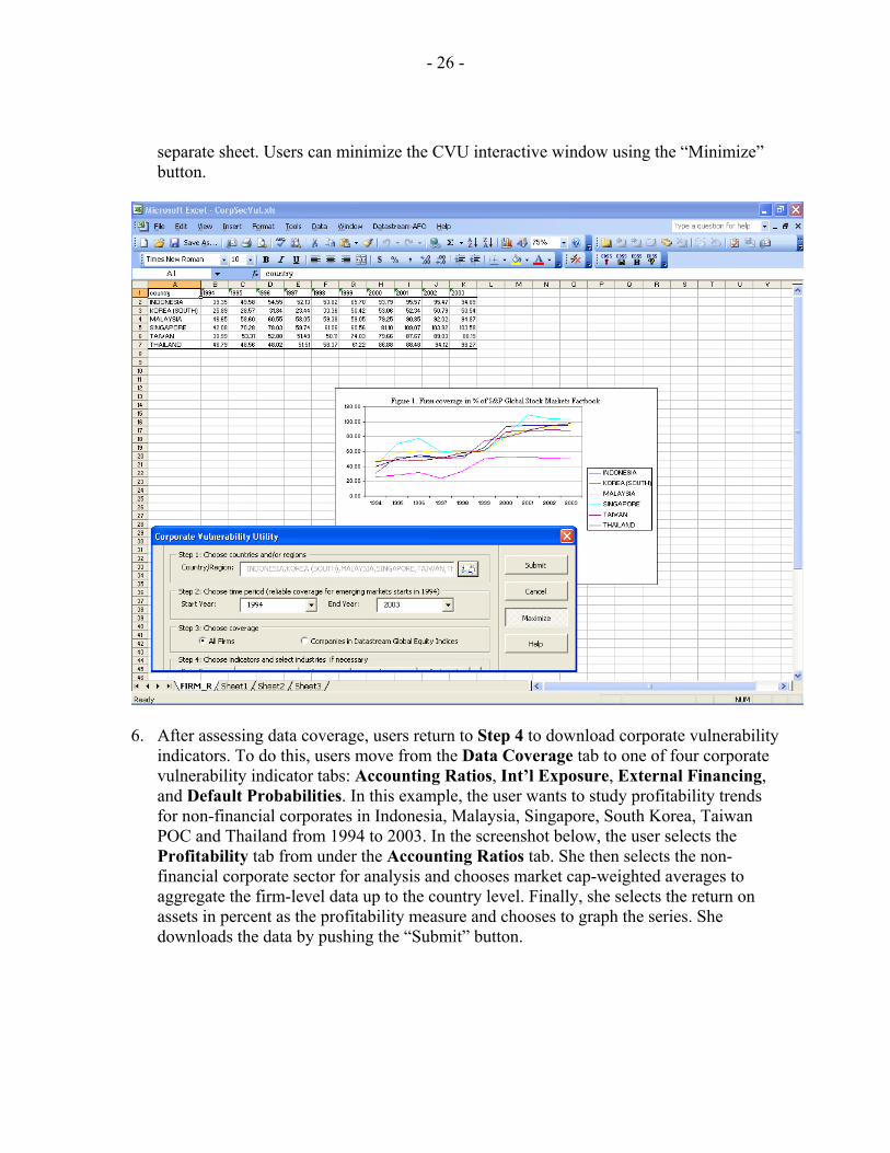
- 26 -

separate sheet. Users can minimize the CVU interactive window using the “Minimize” button.

6. After assessing data coverage, users return to Step 4 to download corporate vulnerability

indicators. To do this, users move from the Data Coverage tab to one of four corporate vulnerability indicator tabs: Accounting Ratios, Int’l Exposure, External Financing, and Default Probabilities. In this example, the user wants to study profitability trends for non-financial corporates in Indonesia, Malaysia, Singapore, South Korea, Taiwan POC and Thailand from 1994 to 2003. In the screenshot below, the user selects the Profitability tab from under the Accounting Ratios tab. She then selects the non-financial corporate sector for analysis and chooses market cap-weighted averages to aggregate the firm-level data up to the country level. Finally, she selects the return on assets in percent as the profitability measure and chooses to graph the series. She downloads the data by pushing the “Submit” button.

- 27 -

7. The screenshot below shows that the CVU downloads the return on assets in percent onto

a separate sheet in Excel. Users can again minimize the CVU interactive window by hitting the “Minimize” button. They can download additional corporate health indicators, which will be downloaded onto separate sheets.

- 28 -

- 29 - APPENDIX I

Data Appendix This appendix describes data sources for all indicators in the CVU. It also contains tables on the cut-offs used to eliminate outliers (Table I), on the number of firms in Datastream indices by country (Table 2), and on the sources for the riskfree rate used in the BSM calculation. Data Coverage

• Number of firms (ACTIVE): number of firms for which fiscal-year-end market cap (WS 08001) and calendar-year-end market cap (DS Code: MV) are greater than zero.

• Market cap in millions of USD (TOTMV): total calendar-year-end market cap (DS

Code: MV) for all firms in ACTIVE.

• Firm coverage in % of S&P Global Stock Markets Factbook (FIRM_R): ACTIVE in % of the number of firms in the Factbook by country.

• Market cap coverage in % of S&P Global Stock Markets Factbook (MK_R): TOTMV

in % of market cap in the Factbook by country.

• Market cap in % of GDP (TOTMV_R): TOTMV in % of GDP from World Economic Outlook (Series Code: NGDP).

Accounting Ratios Leverage

• Debt in % of equity (DE): Worldscope data item (WS 08231).

• Debt in % of assets (DA): Worldscope data item (WS 08236).

• Debt in % of sales (DS): total debt (WS 03255) divided by sales (WS 01001)×100.

• Debt in % of cashflow (TDCF): total debt (WS 03255) divided by cashflow (WS 04201) × 100.

• Short-term debt in % of total debt (STR): short-term debt and current portion of long-

term debt (WS 03051) divided by total debt (WS 03255) × 100.

• Total liabilities in % of assets (TLTA): total liabilities (WS 03351) divided by total assets (WS 02999) × 100.

• Current liabilities in % of total liabilities (CLTL): current liabilities (WS 03101)

divided by total liabilities (WS 03351) × 100.

- 30 - APPENDIX I

• Current assets in % of total assets (CATA): current assets (WS 02201) divided by

total assets (WS 02999) × 100. Liquidity

• Current Ratio (CR): WorldScope data item (WS 08106).

• Quick Ratio (QR): WorldScope data item (WS 08101).

• Cashflow in % of sales (CM): cashflow (WS 04201) divided by sales (WS 01001) × 100.

• Interest coverage ratio (EE): Worldscope data item (WS 08291). • Estimated average interest rate in % (AR): Worldscope data item (WS 08356).

Profitability

• Return on assets in % (RA): WorldScope data item (WS 08326).

• Return on equity in % (RE): WorldScope data item (WS 08371). Valuation

• Price to earnings ratio (PC): Worldscope data item (WS 09104).

• Market to book ratio (BR): Worldscope data item (WS 09704).

• Tobin's Q (TQA): [fiscal-year-end market cap (WS 08001) + book value of total debt (WS 03255)] divided by total assets (WS 02999).

International Exposure

• Foreign sales in % of total sales (FS): Worldscope data item (WS 08731).

• Foreign assets in % of total assets (FA): WorldScope data item (WS 08736).

• Foreign income in % of total income (FI): WorldScope data item (WS 08741). External Financing Indicators The Rajan and Zingales (1998) Index

- 31 - APPENDIX I

• The RZ index (RZ) is made up of five accounting variables: [CE – (CF + DF + DR + PI)] divided by CE × 100:

• Capital expenditures (CE): Worldscope data item (WS 04601), which represents

funds used to acquire fixed assets other than those associated with acquisitions. • Cashflow (CF): Worldscope data item (WS 04201). • Decrease in inventories (DF): -1 × change in inventories (WS 02101). • Decrease in receivables (DR): -1 × change in receivables (WS 02051). • Increase in payables (IP): change in accounts payable (WS 03040).

The Kaplan and Zingales (1997) Index

• The KZ Index (KZ) is a weighted average of five accounting ratios: -1.002*CC + 0.283*TQA + 3.319*DP -39.368*DI -1.315*CP.

• Cashflow / Fixed Assets (CC): cashflow (WS 04201) divided by lagged net property,

plant and equipment (WS 02501). • Tobin's Q (TQA): [fiscal-year-end market cap (WS 08001) + book value of total debt

(WS 03255)] divided by total assets (WS 02999). • Debt / Total Capital (DP): total debt (WS 03255) divided by [total debt (WS 03255) +

total common equity (WS 03501) + preferred stock (WS 03451)]. • Dividends / Fixed Assets (DI): [preferred dividends (WS 05401) + common

dividends (WS 05376)] divided by lagged net property, plant and equipment (WS 02501).

• Cash / Fixed Assets (CP): cash and short-term investments (WS 02001) divided by

lagged net property, plant and equipment (WS 02501). Default Probabilities

The Altman (1968) Z-Score

• The Z-Score is a weighted average of five accounting ratios: 1.2 × Z1 + 1.4 × Z2 + 3.3 × Z3 + 0.6 × Z4 + 0.999 × Z5.

- 32 - APPENDIX I

• Working Capital / Total Assets (Z1): working capital (WS 03151) divided by total assets (WS 02999). (WS 03151) is the difference between current assets and current liabilities.

• Retained earnings / Total Assets (Z2): retained earnings (WS 03495) divided by total

assets (WS 02999). (WS 03495) is accumulated after tax earnings which have not been distributed as dividends to shareholders or allocated to a reserve account.

• EBIT/Total Assets (Z3): EBIT (WS 18191) divided by total assets (WS 02999). (WS

18191) is earnings before interest expense and income taxes by taking the pretax income and adding back interest expense on debt and subtracting interest capitalized.

• Market Value of Equity / Book Value of Total Liabilities (Z4): fiscal-year-end market

cap (WS 08001) divided by total liabilities (WS 03351). • Sales / Total Assets (Z5): sales (WS 01001) divided by total assets (WS 02999).

The Ohlson (1980) O-Score

• The O-Score is a weighted average of nine accounting variables: - 1.32 - 0.407 × O1 + 6.03 × O2 - 1.43 × O3 + 0.076 × O4 - 1.72 × O5 - 2.37 × O6 - 1.83 × O7 + 0.285 × O8 - 0.521 × O9.

• log(Total Assets / GDP deflator) (O1): log[total assets (WS 02999) divided by GDP

deflator index (2000 = 100) obtained from World Economic Outlook (Series Code NGDP_D)].

• Total Liabilities / Total Assets (O2): total liabilities (WS 03351) divided by total

assets (WS 02999).

• Working Capital / Total Assets (O3): working capital (WS 03151) divided by total assets (WS 02999).

• Current Liabilities / Current Assets (O4): current liabilities (WS 03101) divided by

current assets (WS 02201).

• Dummy Variable (O5): one if total liabilities (WS 03351) > total assets (WS 02999), zero otherwise.

• Net Income / Total Assets (O6): net income (WS 01751) divided by total assets (WS

02999).

- 33 - APPENDIX I

• Funds from Operations / Total Liabilities (O7): [pre-tax income (WS 01401) + depreciation and amortization expenses (WS 01151)] divided by total liabilities (WS 03351).

• Dummy Variable (O8): one when there have been two successive years when net

income (WS 01751) < 0, zero otherwise.

• Net Income Growth (O9): [net income (WS 01751) – lagged net income (WS 01751)] / [net income (WS 01751) + lagged net income (WS 01751)].

The Black-Scholes-Merton (BSM) Default Probability

The BSM probability is calculated in Matlab using the Black-Scholes-Merton option pricing formulas. It uses as inputs the following WorldScope and Datastream variables: • SD: short-term debt and current portion of long-term debt (WS 03051).

• LD: total debt (WS 03255) - short-term debt and current portion of long-term debt

(WS 03051).

• IN: standard deviation of return on weekly price index (DS Code: PI) from Datastream, which is annualized by multiplying by sqrt(52).

• MK: fiscal-year-end market cap (WS 08001)

• CD: common dividends (WS 05376).

• ID: interest expense on debt (WS 01251).

• IR: riskfree rate, which is the interest rate on a financial instrument as similar as

possible to the US three month Treasury Bill (see Table 3 in this appendix).

- 34 - APPENDIX I

Table 1. Cut-Off Conditions for Outliers

VariableLower cut-off

conditionUpper cut-off

condition VariableLower cut-off

conditionUpper cut-off

conditionAP AP<0 . O2 O2<0 .AR AR<0 AR>500 O3 . .BP . . O4 O4<0 .BP_US . . O5 . .BR BR<0 . O6 . .BSM BSM<0 BSM>100 O7 . .CA CA<0 . O8 . .CATA CATA<0 CATA>100 O9 . .CC . . OD OD<0 OD>100CD CD<0 . OS . .CE CE<0 . PC PC<-500 PC>500CF CF<0 . PD PD<0 .CI CI<0 . PI . .CL CL<0 . PM PM<-5000 PM>5000CLTL CLTL<0 CLTL>100 PS PS<0 .CM . . PT . .CP CP<0 . QR QR<0 QR>500CR CR<0 CR>500 RA RA<-1000 RA>1000D2 D2<0 . RC . .DA DA<0 . RE RE<-1000 RE>1000DC DC<0 . RZ RZ<-5000 RZ>5000DE DE<0 . SA SA<0 .DEN . . SD SD<0 .DF . . SS SS<0 .DI DI<0 . STR STR<0 STR>100DP DP<0 . TA TA<0 .DR . . TD TD<0 .DS DS<0 . TDCF TDCF<0 TDCF>10000DTD . . TE TE<0 .EA EA<0 . TI TI<0 .EE EE<-5000 EE>5000 TL TL<0 .EQ EQ<0 . TLTA TLTA<0 TLTA>1000ET . . TQA TQA<0 TQA>100FA FA<0 FA>100 TR TR<0 .FD . . VOL . .FI FI<0 FI>100 WC . .FS FS<0 FS>100 XP XP<0 .ID ID<0 . Z1 . .IN IN<0 . Z2 Z2<0 .KZ KZ<-1000 KZ>1000 Z3 . .LD . . Z4 Z4<0 .MK MK<=0 . Z5 Z5<0 .MV MV<=0 . ZD ZD<0 ZD>100NI . . ZS . .O1 . .

- 35 - APPENDIX I

Table 2. Number of Stocks for Datastream Global Equity Indices

Country Approximate No. of Stocks

Base date

Argentina 50 Jan 1988Australia 160 Jan 1973Austria 50 Jan 1973Belgium 90 Jan 1973Brazil 100 July 1994Canada 250 Jan 1973Chile 50 Jul 1989China 100 Sept 1991Colombia 50 Jan 1992Czech Republic 50 Nov 1993Denmark 50 Jan 1973Finland 50 Mar 1988France 250 Jan 1973Germany 250 Jan 1973Greece 50 Jan 1988Hungary 50 June 1991Hong Kong 130 Jan 1973India 100 Jan 1990Indonesia 50 Apr 1990Ireland 50 Jan 1973Israel 50 Jan 1992Italy 160 Jan 1973Japan 1000 Jan 1973Korea 100 Jan 1987Luxembourg 35 Feb 1992Malaysia 90 Jan 1986Mexico 90 Jan 1988Netherlands 130 Jan 1973New Zealand 50 Jan 1988Norway 50 Jan 1980Pakistan 50 Dec 1996Philippines 50 Sep 1987Peru 50 Jan 1994Poland 50 Mar 1994Portugal 50 Jan 1990Romania 50 Dec 1996Russia 50 June 1994Singapore 100 Jan 1973South Africa 70 Jan 1973Spain 120 Jan 1986Sri Lanka 50 June 1987Sweden 70 Jan 1982Switzerland 150 Jan 1973Taiwan 70 Sep 1987Thailand 50 Jan 1987Turkey 50 Jan 1988UK 550 Jan 1965US 1000 Jan 1973Venezuela 20 Jan 1990

- 36 - APPENDIX I

Table 3. Sources for Riskfree Rate

Country Main Source Alternative SourceARGENTINA DX: WALR PC 30 DAY MINIMUMAUSTRALIA For 1990-1992: EDSS: 19361TB.ZB... For 1993-2004: EDSS: 19361.A..XI...AUSTRIA DS: ASVIB3MBELGIUM EDSS: 12460C..ZF...BRAZIL For 1990-1994: DS: BROVERN For 1995-2004: EDSS: 22360C..ZF...CANADA DS: CDN3MTBCHILE* Before July 1997: DX: 90 DAY PRBC For July 1997 and thereafter: DX: 90 DAY PDBCCHINA DS: CHDIS3MCOLOMBIA DS: CBFTDEPCZECH REPUBLIC EDSS: 93560C..ZF...DENMARK DS: DNREPOREGYPT EDSS: 46960C..ZF...FINLAND DS: FNIBC3MFRANCE For 1990-2000: EDSS: 13260C..ZF... For 2000-2004: DS: BBFRF3MGERMANY EDSS: 13460C..ZF...GHANA EDSS: 65260C..ZF...GREECE EDSS: 17460C..ZF...HONG KONG EDSS: 53260C..ZF...HUNGARY EDSS: 94460C..ZF...INDIA For 1990-1992: EDSS: 53460B..ZI... For 1993-2004: DS: INTB91DINDONESIA DS: IDSB90IRELAND DS: EIRED3MISRAEL EDSS: 43660C..ZF...ITALY EDSS: 13660C..ZF...JAPAN DS: JPGBD3MKOREA (SOUTH) DS: KOCD91DLUXEMBOURG EDSS: 12460C..ZF...MALAYSIA DS: MYIBK3MMEXICO EDSS: 27360C..ZF...MOROCCO DS: MDDEP3MNETHERLANDS DS: HOLIB3MNEW ZEALAND DS: NZTBL3MNORWAY DS: NWIBK3MPAKISTAN EDSS: 56460B..ZI...PERU For 1990-2000: EDSS: 29360L..ZB... For 2000-2004: DS: PSDP180PHILIPPINES EDSS: 56660..ZF...POLAND For 1990-2000: EDSS: 96460C..ZF... For 2000-2004: DS: POIBK6MPORTUGAL For 1990-1993: EDSS: 18260C..ZF... For 1994-2004: DS: BPPTE3MRUSSIAN FEDERATION DS: RSIBK90SINGAPORE DS: SNGTB3MSLOVAKIA DS: SXIBK3MSLOVENIA EDSS: 96160C..ZF...SOUTH AFRICA EDSS: 19960C..ZF...SPAIN EDSS: 18460C..ZF...SRI LANKA DS: SRTBL3MSWEDEN Except 2001: EDSS: 14460C..ZI... For 2001 only: EDSS: 14460CBAZB...SWITZERLAND EDSS: 14660C..ZF...TAIWAN DS: TAMM90DTHAILAND For 1990-1993: EDSS: 57860L..ZI... For 1994-2004: DS: THBTRP3TURKEY EDSS: 18660LC.ZB...UNITED KINGDOM EDSS: 11260C..ZI...UNITED STATES DS: USTBL3MVENEZUELA DS: VEN30DPZIMBABWE EDSS: 69860C..ZF..

*Chile's yearly numbers are the simple means of its monthly figures.**EDSS refers to IMF's Economic Data Sharing System, DS stands for Datastream from Datastream International Limited,and DX is a time series system from EconData Pty Ltd.