UNITED NATIONS CONFERENCE ON TRADE AND DEVELOPMENT

POLICY ISSUES IN INTERNATIONAL TRADE AND COMMODITIES

STUDY SERIES No. 24

USER MANUAL AND HANDBOOK ON AGRICULTURAL TRADE POLICY SIMULATION MODEL

(ATPSM)

by

Ralf Peters and David Vanzetti

Trade Analysis Branch Division on International Trade in Goods and Services, and Commodities

United Nations Conference on Trade and Development Geneva, Switzerland

UNITED NATIONS

New York and Geneva, 2004

ii

NOTE

The purpose of this series of studies is to analyze policy issues and to stimulate discussions in the area of international trade and development. The series includes studies by UNCTAD staff, as well as by distinguished researchers from academia. In keeping with the objective of the series, authors are encouraged to express their own views, which do not necessarily reflect the views of the United Nations.

The designations employed and the presentation of the material do not imply the expression of any opinion whatsoever on the part of the United Nations Secretariat concerning the legal status of any country, territory, city or area, or of its authorities, or concerning the delimitation of its frontiers or boundaries.

Material in this publication may be freely quoted or reprinted, but acknowledgement is requested, together with a reference to the document number. It would be appreciated if a copy of the publication containing the quotation or reprint were sent to the UNCTAD secretariat:

Chief

Trade Analysis Branch Division on International Trade in Goods and Services, and Commodities

United Nations Conference on Trade and Development Palais des Nations CH-1211 Geneva

Series Editor: Sam Laird

Officer-in-Charge, Trade Analysis Branch DITC/UNCTAD

UNCTAD/ITCD/TAB/25

UNITED NATIONS PUBLICATION Sales No. E.04.II.D.3 ISBN 92-1-115609-6

ISSN 1607-8291

© Copyright United Nations 2004 All rights reserved

iii

Disclaimer UNCTAD declines all responsibility for errors and deficiencies in the database or software or in the documentation accompanying it, for program maintenance and upgrading as well as for any damage that may arise from them. UNCTAD also declines any responsibility for updating the data and assumes no responsibility for errors and omissions in the data provided. Users are, however, requested to report any errors or deficiencies in the product to UNCTAD. Copyright Copyright © 2004 UNCTAD United Nations Conference on Trade and Development. All rights reserved. ATPSM can freely be used and distributed. Any publications that are partly based on ATPSM must acknowledge the use of ATPSM.

iv

ACKNOWLEDGEMENTS

This handbook was prepared by David Vanzetti and Ralf Peters of the Trade Analysis Branch, UNCTAD. Brett Graham and Odd Gulbrandsen contributed to earlier versions of the handbook. Jenifer Tarcardon-Mercado assisted in the preparation of the manuscript. The model and the handbook were developed in collaboration with the United Nations Food and Agricultural Organization (FAO). UNCTAD received financial support from the United Kingdom Department for International Development (DFID).

v

ABSTRACT

The Agricultural Trade Policy Simulation Model (ATPSM) is designed of detailed

analysis of agricultural trade policy issues. It can be used as a tool by researchers and negotiators alike for quantifying the economic effects at the global and regional level of recent changes in national trade policies.

ATPSM is a deterministic, partial equilibrium, comparative static model covering 161

countries and 35 agricultural commodities. Features of the model include the extensive database, the distinction between bound and applied tariffs, and quota rents. Rents associated with two-tier tariff rate quotas are explicitly modelled within ATPSM. The model solution gives estimates of the changes in trade volumes, prices, government revenues and welfare indicators associated with changes in the trade policy environment. The model is distributed for free from UNCTAD's website at www.unctad.org/tab.

Instructions in the use of ATPSM are contained in this report. No prior knowledge of

modelling or programming is required to install and run the model. The instructions cover use of the interface to set up scenarios and report the results, the model structure and the data.

vi

vii

CONTENTS

USER MANUAL................................................................................................................. ix Installation................................................................................................................. ix Getting started with ATPSM...................................................................................... x Scenarios ...................................................................................................................xi Country groups........................................................................................................xiv HANDBOOK........................................................................................................................ 1 PART A. INTRODUCTION............................................................................................... 2 A.1. Modelling agricultural trade policies................................................................ 2 A.2. The origins of ATPSM ..................................................................................... 2 A.3. ATPSM: A deterministic comparative static partial equilibrium model.......... 2 A.4. Quantifiable and non-quantifiable trade policies ............................................. 3 A.5. Overview of the content of the Handbook........................................................ 3 A.6. Changes to ATPSM since Version 1.1 ............................................................. 4 PART B. A NON-TECHNICAL DESCRIPTION OF ATPSM ..................................... 5 B.1 Country coverage.............................................................................................. 5 B.2. Commodity coverage........................................................................................ 6 B.3. Trade policies included..................................................................................... 6 B.4. Economic estimates .......................................................................................... 7 B.5. Interpretation of the economic effects .............................................................. 7 B.6. Specification of trade policies .......................................................................... 7 B.7. Tariffs and prices .............................................................................................. 8 B.8. Quotas ............................................................................................................... 9 B.8.1. Tariff quotas and quota rents.............................................................. 9 B.8.2. Preference arrangements .................................................................. 11 B.8.3. Export subsidies and quotas ............................................................. 11 B.9. Domestic support ............................................................................................ 12 B.10. Analysing economic effects of trade policy proposals................................... 12 B.11. Model limitations............................................................................................ 14 PART C. ATPSM EQUATIONS AND PROCEDURES............................................... 15 C.1. Main features of ATPSM ............................................................................... 15 C.2. Domestic price formation ............................................................................... 15 C.3. Equation system for individual commodity and country................................ 16 C.4. World market clearing prices ......................................................................... 18 C.5. Trade revenue and welfare effects.................................................................. 19 C.6. Animal product – feed relationships............................................................... 20 C.7. Tariff quota rents and tariff revenues ............................................................. 21

viii

PART D. THE ATPSM DATABASE.............................................................................. 23 D.1. Country list ..................................................................................................... 23 D.2. Prices and volumes ......................................................................................... 23 D.3. Bilateral trade flows........................................................................................ 23 D.4. Tariffs and tariff quotas .................................................................................. 24 D.5. Export subsidies.............................................................................................. 24 D.6. Domestic support ............................................................................................ 24 D.7. Price elasticities .............................................................................................. 25

REFERENCES................................................................................................................... 26 APPENDIX I – ATPSM regions and commodity codes ................................................ 27 A.1. ATPSM region codes ...................................................................................... 27 A.2. ATPSM FAO commodity concordance .......................................................... 29 Figure 1. Quota rents with a binding out-of-quota tariff................................................ 10

ix

USER MANUAL

Agricultural Trade Policy Simulation Model (ATPSM Version 3, August 2004)

Installation

ATPSM Version 3 can be downloaded free of charge from the UNCTAD website at

http://www.unctad.org/tab/ and automatically installed by running the installation program. It may also be installed from a CD available from the Trade Analysis Branch at UNCTAD. To start the program the user will need merely to click on an icon on the desktop.

ATPSM may need to be installed manually in some situations, for example if the program

has been obtained via e-mail. Manual installation instructions: Unzip the zip file to any folder, keeping the folder structure within it. It is useful to keep the

database file atpsm.mdb in a separate folder to prevent it being overwritten with subsequent updates. The main installation task is to create a link to this database as follows:

Create an ODBC data source called atpsm using the file atpsm.mdb:

Control Panel Administrative Tools Data Sources (ODBC) Add Button select Microsoft Access Driver (*.mdb) Finish button Data Source Name = atpsm Click Select and find the file atpsm.mdb Ok Then just double-click on atpsm.exe in the Explorer to open the model. A shortcut can be

created by right-clicking on this file.

To check that the Microsoft Access database file atpsm.mdb is correctly linked, go to the scenarios page and click on "All countries" under the heading "Country code". A long list of countries should appear. If not, try the ODBC data source linking procedure again.

Help files are provided via the menu. Previous scenarios can be loaded, or new ones created

by entering the shocks, saving the scenario definition and pressing "simulate". When the simulation is "finished" go to the results.

x

Getting started with ATPSM

ATPSM is a trade policy simulation model. It can be used as a tool for quantifying economic effects of changes in trade policies. The user specifies a specific change in trade policy, the model simulates the new prices and trade flows and calculates welfare effects. The results can be analysed and saved by the user.

General information about ATPSM, its structure and functionality, can be obtained from the ATPSM Handbook.

ATPSM has a graphical user interface to assist the user in setting up scenarios, running the simulations and storing and reading the output data. Context-specific on-line help is available.

Instructions on using the graphical user interface are given here. Instructions on how to run a simulation and how to check results are given at the on-line help pages belonging to Scenarios and Results.

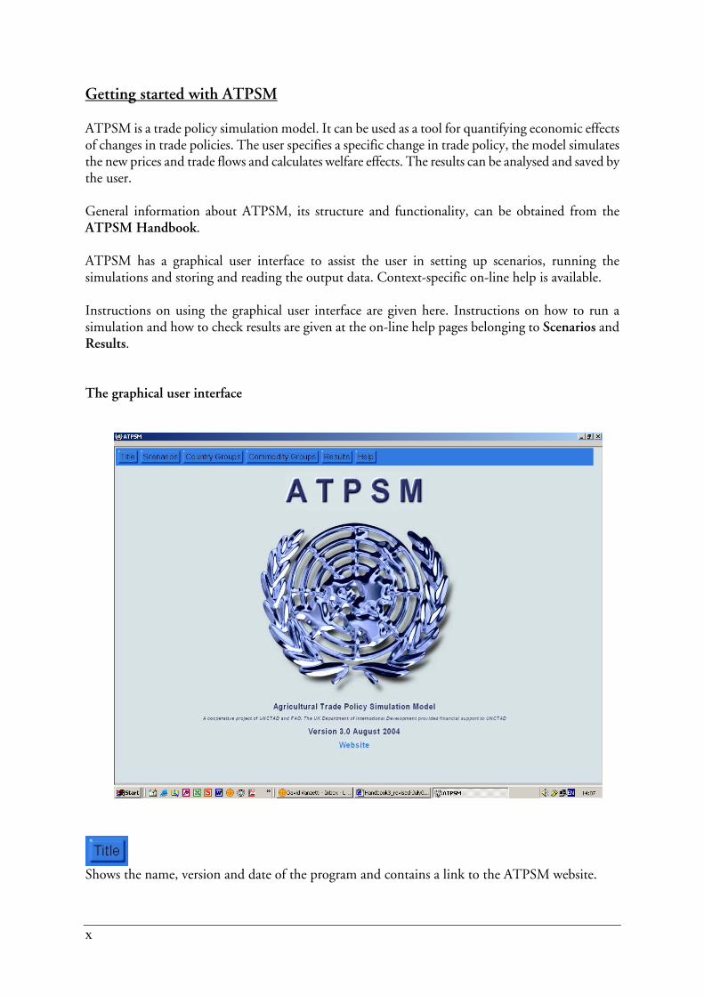
The graphical user interface

Shows the name, version and date of the program and contains a link to the ATPSM website.

xi

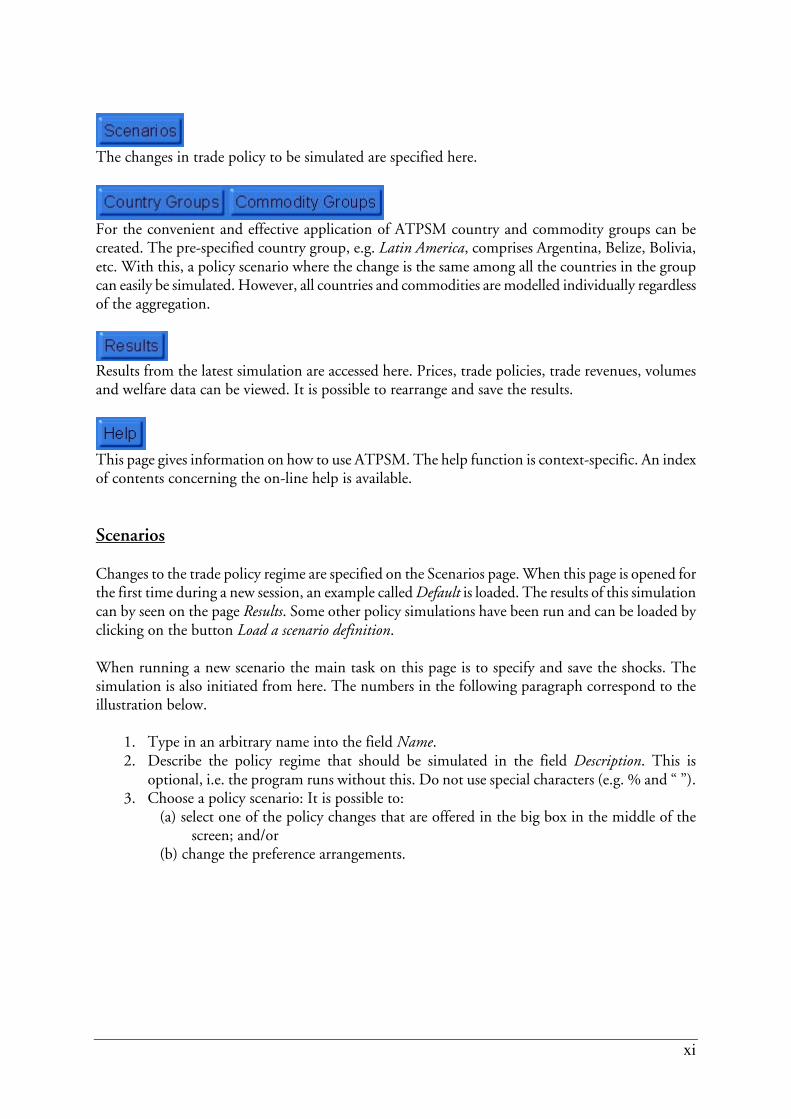
The changes in trade policy to be simulated are specified here.

For the convenient and effective application of ATPSM country and commodity groups can be created. The pre-specified country group, e.g. Latin America, comprises Argentina, Belize, Bolivia, etc. With this, a policy scenario where the change is the same among all the countries in the group can easily be simulated. However, all countries and commodities are modelled individually regardless of the aggregation.

Results from the latest simulation are accessed here. Prices, trade policies, trade revenues, volumes and welfare data can be viewed. It is possible to rearrange and save the results.

This page gives information on how to use ATPSM. The help function is context-specific. An index of contents concerning the on-line help is available.

Scenarios

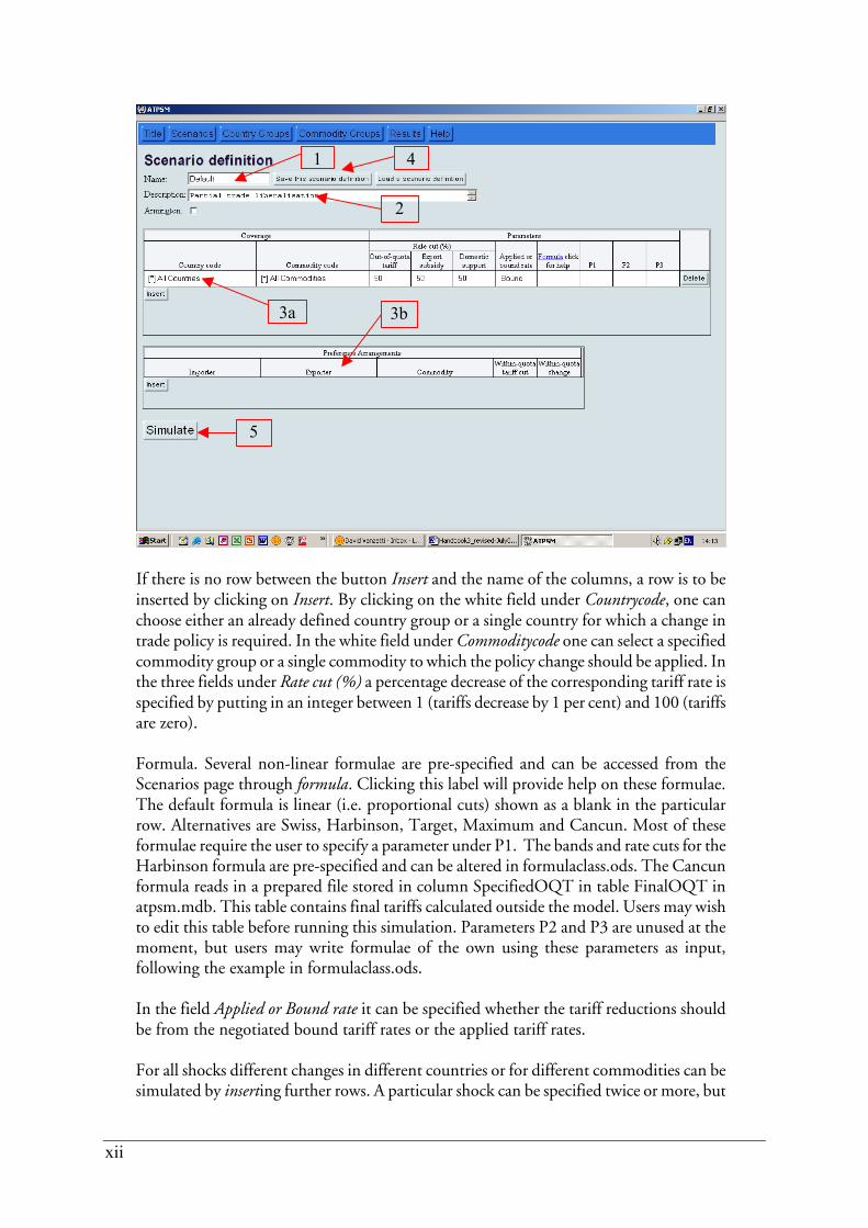
Changes to the trade policy regime are specified on the Scenarios page. When this page is opened for the first time during a new session, an example called Default is loaded. The results of this simulation can by seen on the page Results. Some other policy simulations have been run and can be loaded by clicking on the button Load a scenario definition.

When running a new scenario the main task on this page is to specify and save the shocks. The simulation is also initiated from here. The numbers in the following paragraph correspond to the illustration below.

1. Type in an arbitrary name into the field Name. 2. Describe the policy regime that should be simulated in the field Description. This is

optional, i.e. the program runs without this. Do not use special characters (e.g. % and “ ”). 3. Choose a policy scenario: It is possible to:

(a) select one of the policy changes that are offered in the big box in the middle of the screen; and/or

(b) change the preference arrangements.

xii

If there is no row between the button Insert and the name of the columns, a row is to be inserted by clicking on Insert. By clicking on the white field under Countrycode, one can choose either an already defined country group or a single country for which a change in trade policy is required. In the white field under Commoditycode one can select a specified commodity group or a single commodity to which the policy change should be applied. In the three fields under Rate cut (%) a percentage decrease of the corresponding tariff rate is specified by putting in an integer between 1 (tariffs decrease by 1 per cent) and 100 (tariffs are zero).

Formula. Several non-linear formulae are pre-specified and can be accessed from the Scenarios page through formula. Clicking this label will provide help on these formulae. The default formula is linear (i.e. proportional cuts) shown as a blank in the particular row. Alternatives are Swiss, Harbinson, Target, Maximum and Cancun. Most of these formulae require the user to specify a parameter under P1. The bands and rate cuts for the Harbinson formula are pre-specified and can be altered in formulaclass.ods. The Cancun formula reads in a prepared file stored in column SpecifiedOQT in table FinalOQT in atpsm.mdb. This table contains final tariffs calculated outside the model. Users may wish to edit this table before running this simulation. Parameters P2 and P3 are unused at the moment, but users may write formulae of the own using these parameters as input, following the example in formulaclass.ods.

In the field Applied or Bound rate it can be specified whether the tariff reductions should be from the negotiated bound tariff rates or the applied tariff rates. For all shocks different changes in different countries or for different commodities can be simulated by inserting further rows. A particular shock can be specified twice or more, but

1

2

3b 3a

4

5

xiii

latter rows overwrite earlier rows. For example, if All commodities are specified in the first row and Sugar in the second, the latter is read last. The button Delete deletes single rows. If there is no row between the button Insert and the name of the columns, a row is to be inserted by clicking on Insert.

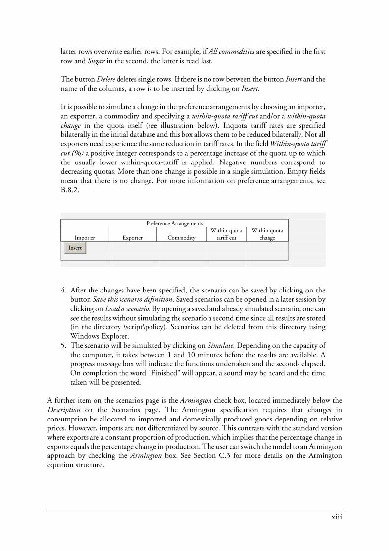
It is possible to simulate a change in the preference arrangements by choosing an importer, an exporter, a commodity and specifying a within-quota tariff cut and/or a within-quota change in the quota itself (see illustration below). Inquota tariff rates are specified bilaterally in the initial database and this box allows them to be reduced bilaterally. Not all exporters need experience the same reduction in tariff rates. In the field Within-quota tariff cut (%) a positive integer corresponds to a percentage increase of the quota up to which the usually lower within-quota-tariff is applied. Negative numbers correspond to decreasing quotas. More than one change is possible in a single simulation. Empty fields mean that there is no change. For more information on preference arrangements, see B.8.2.

Preference Arrangements

Within-quota Within-quota

Importer Exporter Commodity tariff cut change

Insert

4. After the changes have been specified, the scenario can be saved by clicking on the button Save this scenario definition. Saved scenarios can be opened in a later session by clicking on Load a scenario. By opening a saved and already simulated scenario, one can see the results without simulating the scenario a second time since all results are stored (in the directory \script\policy). Scenarios can be deleted from this directory using Windows Explorer.

5. The scenario will be simulated by clicking on Simulate. Depending on the capacity of the computer, it takes between 1 and 10 minutes before the results are available. A progress message box will indicate the functions undertaken and the seconds elapsed. On completion the word "Finished" will appear, a sound may be heard and the time taken will be presented.

A further item on the scenarios page is the Armington check box, located immediately below the Description on the Scenarios page. The Armington specification requires that changes in consumption be allocated to imported and domestically produced goods depending on relative prices. However, imports are not differentiated by source. This contrasts with the standard version where exports are a constant proportion of production, which implies that the percentage change in exports equals the percentage change in production. The user can switch the model to an Armington approach by checking the Armington box. See Section C.3 for more details on the Armington equation structure.

xiv

Country groups Users can create country groups to more conveniently specify shocks and report input and

output. However, for the purpose of the simulation countries within groups are treated separately. To create a new group:

1. Click on Country Groups or Commodity Groups in the main menu. 2. Enter an arbitrary code of a few letters or numbers in the field Code and enter a country

group name in the field Name. 3. Click insert. 4. Highlight the new group name in the window Currently defined groups. 5. Click on the button Countries. 6. Add countries to the group by clicking on the sign in front of a country in the window on

the left-hand side. 7. Countries can be deleted by clicking on the sign in front of a country in the window on

the right-hand side. 8. It is not necessary to confirm or save the input.

The new defined groups remain available after the end of a session. There are several predefined country groups. A list of predefined groups can be seen in the

ATPSM Handbook, B.1. Results

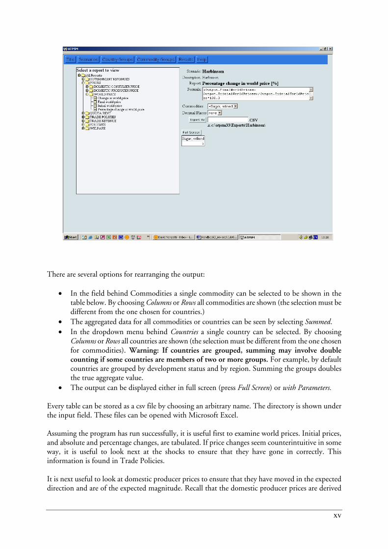
Results on prices, trade policies, trade revenues, volumes and welfare data from the latest simulation are accessed here. Click on the plus sign to see the contents of the categories. A table can be opened by pressing the corresponding button .

The output shows the chosen name of the scenario, a description of the proposal, the name of the variable displayed and the formula with which the output is calculated within the program. The latter may be changed by editing the text box containing the formula. For example, values can be expressed in millions by dividing by 1000000.0 (e.g. write: (Output.FinalWorldPrices-Output.InitialWorldPrices)/1000000.0). However, the labelling will not reflect the modified formula.

xv

There are several options for rearranging the output:

• In the field behind Commodities a single commodity can be selected to be shown in the table below. By choosing Columns or Rows all commodities are shown (the selection must be different from the one chosen for countries.)

• The aggregated data for all commodities or countries can be seen by selecting Summed. • In the dropdown menu behind Countries a single country can be selected. By choosing

Columns or Rows all countries are shown (the selection must be different from the one chosen for commodities). Warning: If countries are grouped, summing may involve double counting if some countries are members of two or more groups. For example, by default countries are grouped by development status and by region. Summing the groups doubles the true aggregate value.

• The output can be displayed either in full screen (press Full Screen) or with Parameters.

Every table can be stored as a csv file by choosing an arbitrary name. The directory is shown under the input field. These files can be opened with Microsoft Excel.

Assuming the program has run successfully, it is useful first to examine world prices. Initial prices, and absolute and percentage changes, are tabulated. If price changes seem counterintuitive in some way, it is useful to look next at the shocks to ensure that they have gone in correctly. This information is found in Trade Policies.

It is next useful to look at domestic producer prices to ensure that they have moved in the expected direction and are of the expected magnitude. Recall that the domestic producer prices are derived

xvi

from a blend of the import tariffs and export subsidies. The domestic price change is a result of the world price change and the exogenously determined trade policy change. Hence, the domestic producer price may either rise or fall. The user may then read and analyze trade revenues, volumes of consumption, production, exports and imports, as well as welfare effects. Bilateral (country to country) information is shown for quotas, rent and within-quota tariffs. Menus for importers and exporters are shown on the interface. To avoid a delay in presenting bilateral three dimensional information, it is useful to limit one dimension (importer, exporter or commodity) to a single element.

HANDBOOKAgricultural Trade Policy Simulation Model

(ATPSM Version 3, August 2004)

2

A.1. Modelling agricultural trade policies

The Agricultural Trade Policy Simulation Model (ATPSM) is a trade policy simulation modelcapable of detailed analysis of agricultural trade policy issues. It can be used as a tool by researchersand negotiators alike for quantifying the economic effects at the global and regional levels ofrecent changes in national trade policies. Alternatively, it can be used to consider the potentialchanges resulting from future unilateral action by individual countries or actions required undernegotiated agreements.

ATPSM is a deterministic, partial equilibrium, comparative static model. It analyses theeffects of price and trade policy changes on supply and demand using a system of simultaneousequations that are characterized by a number of data and behavioural relationships designed tosimulate the real world. The model solution gives estimates of the changes in trade volumes,prices and welfare indicators associated with changes in the trade policy environment. A feature ofthe model is its handling of a two-tier tariff structure whereby imports within a quota level attracta relatively low tariff, and out-of-quota imports face a higher tariff. Rents associated with thesequotas are explicitly modelled within ATPSM.

Given limitations in the data and the abstract nature of such models, the user should interpretthe results with caution. However, the model has detailed commodity and country coverage andfor the comparison of various policy scenarios, it can be very helpful in indicating the relativemagnitudes of the effects of policy changes on welfare, trade and prices.

A.2. The origins of ATPSM

The development of ATPSM was initiated by UNCTAD in 1988. A detailed description ofthe model and its results was published for the first time in 1990 in a United Nations studyentitled, Agricultural Trade Liberalization in the Uruguay Round: Implications for Developing Countries(UNCTAD/ITP/48).

In the late 1990s, the model was significantly enhanced in a joint effort by UNCTAD, withfunding from the United Kingdom Department for International Development, and the Food andAgriculture Organization of the United Nations (FAO) to address issues arising from the outcomeof the Uruguay Round. The model database coverage was increased to enable policy analysis in anincreasing number of commodities and countries. The model equations were refined to enable theanalysis of changes in tariff quotas and tariff quota rates and to distinguish between bound andapplied tariff rates.

A.3. ATPSM: A deterministic comparative static partial equilibrium model

The model consists of a system of equations that represent supply, demand and trade flowsfor different agricultural goods in different countries.

PART A: INTRODUCTION

3

In an attempt to simulate the real world a number of assumptions are made. The model isdeterministic. There are no stochastic shocks or other uncertainties. It is static. There is no specifictime dimension to the implementation of policy measures or to the maturing of their economiceffects. Finally, it is a partial equilibrium model. Whereas the model aims at estimating far-reachingdetails of the agricultural economy, it does not deal with the repercussions of barrier reductions onother parts of the national economy. Thus, effects on the industrial and service parts of the economyor the labour market are not subject to analysis.

Simplifying the model in these respects allows a detailed specification of the most relevantagricultural trade policies having computable economic effects. Similarly, the model reports resultsfor many different countries. It gives results not only globally but also for various country groups,geographical as well as political. There is extensive coverage of agricultural commodities and themodel considers interrelationships between the agricultural commodities in both supply and demand(for example, when competing for land or consumer preferences). Finally, the model accounts forthree different economic agents within each economy – producers, consumers and government.Therefore, results can be presented by commodity and by agent for each country, each region orthe world.

A.4. Quantifiable and non-quantifiable trade policies

The ATPSM focuses on standard agricultural trade policies, such as tariff cuts, subsidyreductions and quota changes. However, a number of other agricultural trade interventions exist,such as sanitary and phytosanitary regulations, seasonal import restrictions and anti-dumpingmeasures. Such interventions cannot be simulated unless a tariff equivalent can be derived.

Another set of non-quantifiable policies is found in the farm price support over and abovethe market access measures. These range from subsidies on agricultural inputs to research anddevelopment financing, favourable interest rates and amortization periods on loans etc. The primaryproblem in modelling such policies is that the support they provide is general and not specificallyassigned to certain commodities. These policies support agricultural production capacity as a whole.Although one could envisage simulating such support in a model, it is not currently possible in theATPSM.

A.5. Overview of the content of the Handbook

This Handbook is prepared with two main purposes:

- to facilitate the understanding of the model’s capabilities and outcome of policy scenarios;- to allow users to formulate policy scenarios, execute the model and interpret the results.

The Handbook is structured as follows: Part B of this Handbook provides a non-technicaldescription of the ATPSM. The countries, commodities and policies that are included in themodel are specified and defined. Details on policies related to market access, import quota rents,export subsidies, domestic support and bilateral quotas are provided. An explanation on how tointerpret the results is presented.

4

Part C of the Handbook provides details on how to operate the model. The main features ofthe model, implementing trade policy scenarios and reading the output are outlined. Since ATPSMhas a graphical user interface with context-specific online help, further features are addressed briefly.

Part D of the Handbook provides a detailed mathematical description of the model. Technicalissues relating to trade equilibrium, domestic price determination, quota rents and feedshare effectsare explained.

A.6. Changes to ATPSM since Version 1.1

The current (August 2004) version of ATPSM is 3. In this version several changes to thedatabase have been implemented:

(i) Several commodities have been removed or aggregated (coffee, tobacco) and otherssplit (sugar) or added (livestock, rubber).

(ii) Volume data have been updated to the average of three years 1999-2001.(iii) Price data have been updated to 1999-2001.(iv) Applied tariff data have been updated to 2001 or 2000.(v) Export subsidy data have been revised and now include the value of export credits. In

addition, reductions in exports subsidies now depend on the volume and expenditureconstraints, just as applied tariff reductions depend on the difference between boundand applied tariffs.

(vi) Bilateral in-quota tariff data have been included, so in-quota tariff reductions can bespecified bilaterally.

(vii) Elasticities have been revised to include more cross-elasticities. These are derived fromown price elasticities plus various axioms (homogeneity, symmetry, Slutzky condition).

(viii) Capture rates are specified in the database. Rents are assumed to accrue to producerswhere tariff rate quotas are allocated historically.

There have been a number of cosmetic changes to the graphical user interface:

(i) In-quota tariffs can be specified and reported bilaterally.(ii) Users can specify their own tariff-cutting proposals in a customized formula box.(iii) A progress box is included to indicate running time.(iv) An Armington toggle is included on the interface so users can choose how two-way

trade is determined.(v) Commas are inserted between thousands and millions to improve clarity.(vi) Negative numbers have a minus (-) sign, and are no longer in red.

Details of recent changes are given in the table xxDataModifications in the ATPSM Accessdata file atpsm.mdb.

Version 3 contains modifications to the data, script and executable files. Users of previousversions of ATPSM can update without having to install the program again. New files can merelybe copied over the previous version. The new database file atpsm.mdb should be placed in thesame folder as the previous one so that the link to the database is maintained. After changing thedata file, the saved scenarios have to be rerun if the user is still interested in their results.

5

The ATPSM has a global coverage of agricultural commodities with protection barriers thatsignificantly distort world trade. It estimates the effects of barrier reductions on terms of trade,tariff revenues, welfare, supply and demand allocation and prices. It takes into account almost allthe agricultural trade policy measures having computable economic effects.

B.1. Country coverage

The present version of the model covers 176 countries and includes all larger economies.The countries that are not explicitly covered by the model are mostly small island economies andare included in the Rest of World. The economy of each country is represented individually, exceptthe 15 countries that are part of European Union which are represented as a single country group.

The lack of agricultural trade policy data prevents extended policy analysis for some countries.In the present version of the model, no policy data are available for 20 countries. For a further 37countries there are either no applied or no bound tariff rates available. These countries are essentiallyprice takers in the model, with domestic prices moving with world prices and production,consumption, exports and imports adjusting accordingly. Country coverage is found in AppendixI, table A.1.

For the convenient and effective application of ATPSM it is possible to define one’s owncountry and commodity groups. This can be done on the pages Country Groups and CommodityGroups. Using these groups in the simulations, the policy changes correspond to all countries orcommodities that belong to the group. The new defined groups remain available after the end of asession.

There are several predefined country and commodity groups available. One category of groupsis the partition in Developed, Developing and Least Developed Countries. Each country in themodel belongs to one of these three groups. Another classification is regional. There are elevenregional groups and, again, every country belongs to one and only one of these eleven groups. Thepredefined regions are:

- Caribbean- Central America- Central and Eastern Europe- Central Asia- North Africa and the Middle East- North America- Oceania- South America- South, East and South-East Asia- Sub-Saharan Africa- Western Europe.

The assignment of countries to groups can be changed by the user.

PART B: A NON-TECHNICAL DESCRIPTION OF ATPSM

6

B.2. Commodity coverage

Many agricultural commodities are subject to agricultural trade policy distortions. Thosewith particularly high barriers having substantially distorting economic impact are the basicfoodstuffs, such as animal and cereal products, sugar, and vegetable oils and oil seeds. Tropicalproducts of interest to developing countries include beverages, cotton and tobacco. Although notpart of the Agreement on Agriculture, rubber is also included in the 35 ATPSM commodities.

The commodities can be aggregated into groups. The predefined commodity groups are:

- Beverages (cocoa, tea, coffee)- Cereals (wheat, rice, barley, maize and sorghum)- Dairy products (milk concentrates, butter and cheese)- Fruit (apples and pears, citrus, bananas and other tropical fruit)- Meat (livestock, bovine meat, sheep meat, pig meat and poultry)- Oilseeds (vegetable oils and oilseeds)- Sugar (sugar, raw and sugar, refined)- Tobacco and cotton (tobacco and cotton)- Vegetables (pulses and roots and tubers, and tomatoes).

The assignment of commodities to groups can be changed by the user. The commodityconcordance is specified in Appendix I, table A.2.

B.3. Trade policies included

While ATPSM can analyse many general trade policy issues, its main purpose is to simulateand evaluate the various agricultural trade policy changes that may be suggested for or in theWTO negotiations on agriculture. The present version can simulate general policy changes commonfor all countries and commodities involved in these negotiations or policy changes specific toindividual countries or groups of countries.

Trade policy changes that can be simulated by the model include:

- Reduction of out-of-quota tariffs, either by a linear percentage reduction or by severalnon-linear formulae, such as the so-called Swiss formula;1

- Reduction of bilateral within-quota tariffs, by a certain percentage;- Reduction of the tariff equivalent of domestic support (over and above market-access

measures), by a certain percentage;- Reduction in the tariff equivalent of export subsidies, by a certain percentage;- Change in bilateral import quotas, by a certain percentage;- Different percentage changes in all the above policies applied to selected countries or country

groups and commodities;- Use of applied tariff rates instead of bound out-of-quota rates.

1 The Swiss formula implies the higher the tariff, the deeper the tariff cut (for example, a 100% tariff is cut by50%, but a 150% tariff is cut by 60%).

7

B.4. Economic estimates

The model produces five categories of economic estimates for each country:

- Volume changes in production consumption, imports and exports;- Trade value changes – changes in export, import and net trade revenue;- Welfare changes – changes in producer surplus, consumer surpluses; and net government

revenue;- Price changes – world market, wholesale (consumer) and farm prices;- Changes in tariff quota rents – forgone and receivable.

The introduction of a two-tier tariff system with import quotas that resulted from the UruguayRound agreement created a new category of economic effects – the tariff quota rents. The capturerate of these rents can be specified by country and commodity from the menu. The default settingin ATPSM is that producers from the exporting country capture 100 per cent of these rents.

Because the model produces figures for all these estimates, by country, by region, bycommodity and by policy scenario, there is considerable scope for the evaluation of trade policyproposals by comparing results from different scenarios. Users can examine the effects on thecountry or commodity that is of primary interest to them. Alternatively, it is possible to concentrateon the overall effects of the trade policy proposals and make recommendations based on an overallanalysis.

B.5. Interpretation of the economic effects

As previously noted, the model does not have a time dimension. Therefore, nothing can beinferred about the time length within which the economic effects would be fully realized. Thegeneral interpretation is that the economic effects are of a long-term nature, with the implementationspread over several years. The elasticities that govern supply and demand responses to price changeshave been estimated on the basis of a 10-year time horizon.

There is a distinct difference in the speed of reaction between demand and supply responseto price changes. The reaction of the former is relatively quick, with full response from one to twoyears. The full response of the latter, however, may be from one to more than ten years, dependingon the commodity. If there were an immediate reduction in trade barriers this imbalance in thetiming of responses could create a temporary disequilibrium. As the lag in supply response wouldbe greater than that in demand there could be an excessive increase in prices or a substantialreduction in the stocks (or both). However, as negotiated reductions in trade barriers are generallyspread over several years, the impact of the potential imbalance resulting from differing responsetimes is likely to be minimal.

B.6. Specification of trade policies

In ATPSM the changes in supply and demand are estimated from percentage changes indomestic prices. To estimate the percentage change in domestic prices from trade policy changesall tariffs must be expressed as a percentage of the world market price. In ATPSM specific andmixed tariffs are converted into ad-valorem equivalents.

8

In ATPSM tariff cuts are expressed as a percentage of the initial tariff. The default method inthe model for implementing tariff cuts is to reduce all tariffs by an equal percentage (linear cuts).However, alternative methods have been suggested and implemented in previous negotiating rounds.One of these methods is the Swiss formula, which makes progressively higher proportional taxcuts in progressively higher tariffs. Global and specific tariff cuts using this method can also besimulated in ATPSM. Other cuts include the Harbinson bands approach and a pre-specified Cancunor blended formula. Final tariffs can also be set to a maximum or to a pre-specified target level.

Export subsidies and extra farm support are measured as tariff ad-valorem equivalents in themodel. Hence, cuts in these supports are measured as percentage reductions of the ad-valoremequivalents.

The model is capable of analysing global trade policy changes, specific trade policy changesto individual countries and commodities or some combination thereof. In any simulation theglobal tariff cuts apply to all countries and commodities that are not assigned specific tariff cuts.

Tariff quotas are expressed in volumes. A policy change is expressed as a percentage changeof the quota. Positive changes in tariff quotas allow more imports to enter under a lower within-quota tariff.

B.7. Tariffs and prices

In the model domestic prices are determined as a function of world market prices and of thesupport measures, tariffs, subsidies and quotas. There is no independent behaviour of domesticprices. Also, no account is taken of domestic trade margins. Domestic prices have the character ofborder wholesale prices. An exception is the farm (supply) price, which might be affected by extrafarm price support (for example, deficiency payments) over and above the market access support.

In the ATPSM datasets a country is often an importer and exporter of the one (aggregated)good. To accommodate this feature of trade data, composite tariffs for determining the domesticconsumption and production price are estimated. This is in contrast with other trade models thatdetermine domestic demand with a nested import demand structure, which requires knowledge ofimport elasticities between all foreign goods, so-called Armington elasticities. These elasticities arenotorious for their importance in determining trade model outcomes, but little detailed quantitativeassessment of them has been done.

The first step to estimate this tariff is to compute a tax on domestically consumed production.This tax is assumed to be a trade-weighted average of the import tariff and the export tariffequivalent. The domestic wholesale price is then estimated as the average of the import tariff andthe tax for the domestically consumed production, weighting the former by imports and the latterby the domestically consumed production. The producer (farm price) is computed as the averageof the export support and the domestically consumed production tax, weighting the former byexports and the latter by the domestically consumed production, plus the tariff equivalent of extrafarm support.

9

One of the attractive properties of this price specification is that where a commodity isexclusively imported, the wholesale and farm price are equal to the world market price plus theimport tariff. Similarly, if the commodity is exclusively exported, the domestic wholesale and farmprice are equal to the world market price plus the tariff equivalent of the export subsidy.

Tariff cuts can be specified for the out-of-quota and within-quota tariff and for the tariffequivalents of export subsidies and extra farm support. If the applied tariff is lower than the policy-determined reduced bound out-of-quota tariff, the former is applied. Alternatively, the user canspecify that tariff cuts be made to the applied rates.

B.8. Quotas

The model can estimate the economic consequences of import quota changes. Import quotasare assumed to be binding. Changing the import quotas exogenously changes the allocation ofquota rents and tariff revenues, but not the level of imports.

B.8.1. Tariff quotas and quota rents

The Agreement on Agriculture of the Uruguay Round instituted a new system of tarifficationthat can be characterized as a general preferential arrangement. The system consists of a two-tiertariffication with a low tariff applying to an import quota (the “within-quota tariff ”) and a hightariff applying above the import quota (the “out-of-quota tariff ”). The importing country controls(although with the obligation to notify the WTO) the size of the quota, referred to as the globalquota, and the distribution of it among suppliers, referred to as bilateral quotas.

This system has the peculiarity of generating rents. Their size makes them an importantdeterminant of welfare and therefore warrants inclusion in the model.

Quota rents are the quota times the difference between the domestic prices and world priceplus the within-quota tariff. There are three possible scenarios:

(1) If the within-quota tariff is binding, the quota is unfilled, domestic prices equal worldprices plus the within-quota tariff and there is no quota rent;

(2) If the quota is binding, imports equal the quota and the rent is positive butindeterminate;

(3) If the over-quota tariff is binding, imports exceed the quota and the rent is the quotatimes the difference between the within-quota and out-of-quota tariff rates.

Ideally, the import quota fill rate should determine the domestic price. If the quota is unfilleddomestic prices should be determined by the within-quota tariffs, and prices should be high onlyif the quota is filled or overfilled. However, it is often observed that quotas are unfilled but domesticprices are high nonetheless. This may be because administrative constraints prevent the quotasbeing filled, or perhaps quotas are allocated on an historical basis to countries that are no longerexporters. More to the point, countries with high domestic prices are unlikely to be prepared to seethem eroded by a shift in the supply of imports. As a result, the assumption here is that the out-of-quota tariffs (or possibly the applied tariffs) determine the domestic market price.

10

This assumption restricts the model in two important ways. Firstly, it is not possible tomodel an increase in import quotas above the initial level of imports. Secondly, changes in quotarents make no impact on the exporting countries’ supply decisions because, on the margin, theprice received by the supplier does not change as quota rents change. The quota rent is effectivelya lump sum transfer from the importing country’s Government to the exporting countries’ supplier.

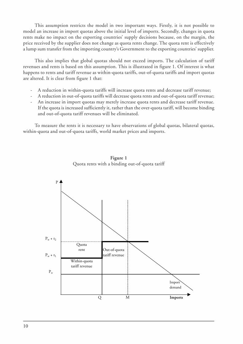
This also implies that global quotas should not exceed imports. The calculation of tariffrevenues and rents is based on this assumption. This is illustrated in figure 1. Of interest is whathappens to rents and tariff revenue as within-quota tariffs, out-of-quota tariffs and import quotasare altered. It is clear from figure 1 that:

- A reduction in within-quota tariffs will increase quota rents and decrease tariff revenue;- A reduction in out-of-quota tariffs will decrease quota rents and out-of-quota tariff revenue;- An increase in import quotas may merely increase quota rents and decrease tariff revenue.

If the quota is increased sufficiently it, rather than the over-quota tariff, will become bindingand out-of-quota tariff revenues will be eliminated.

To measure the rents it is necessary to have observations of global quotas, bilateral quotas,within-quota and out-of-quota tariffs, world market prices and imports.

Figure 1Quota rents with a binding out-of-quota tariff

P

Pw + t2

Out-of-quotaPw + t1 tariff revenue

Pw

Importdemand

Q Imports M

Quotarent

Within-quotatariff revenue

11

Global quotas, specifying the total level of imports at the lower tariff level, are notified to theWTO, but most bilateral quotas are not and have to be estimated. The model uses bilateral tradeflows to estimate the bilateral quota distribution. For each bilateral trade flow of each commoditythe rent is calculated.

Which agent actually captures the rent created by the tariff rate quota depends on institutionalfactors and market structures. Rents could accrue to a number of agents, including exportingproducers, exporting Governments, importing Governments, importing consumers or distributionand processing agents. Alternatively, the rent could be dissipated through unproductive rent-seekingactivities. For a discussion on tariff rate quota administration see Abbott and Morse (1999), deGorter and Sheldon (2000) and Skully (2001).

In ATPSM the capture rate of the rent can be specified by country and by commodity in thecapturerate column in table RentCapture in the database. The rent can be allocated to the supplierand the importing country Government. The capture rate specifies the share in the quota rent, so100 implies all the rent accrues to the exporter.

The model measures the rents forgone by importers, given a 100 per cent rent capture byexporters. Global rents forgone equate with rents receivable. For countries with special preferences,such as the ACP countries that have preferential access to EU markets, rent is equal to the wholeout-of-quota tariff times the bilateral quota.

B.8.2. Preference arrangements

Some countries allow other countries to bring in commodities at reduced or zero tariffs.Users can specify reduction in bilateral tariffs facing exporters with preferential access to specificmarkets. This is only relevant where quota rents accrue to exporters. This is specified by the capturerate. These are contained in the database (see the RentCapture table in atpsm.mdb or the variableinitial quota rent to exporter in the results tab on the interface) and may be respecified by the user.

B.8.3. Export subsidies and quotas

Export subsidies and export quotas are intrinsically linked in ATPSM. If the export quotadetermines the size of exports, the unit tariff of the export support is equal to the subsidy dividedby the quota. The ad-valorem tariff equivalent is the ratio of the unit tariff to the world marketprice. However, if exports exceed the quota, the subsidy becomes simply a transfer of wealth as, onthe margin, the additional exports are sold at world market prices and eliminate the domesticmarket protection. In such a case it is assumed that the subsidy extends to total exports. The unittariff is then calculated as the total value of the subsidy divided by the export volume.

This treatment ignores two possible complications in the application of export subsidies. Itis possible that an export subsidy is applied at a lower rate than the import tariff on the samecommodity, this making the export subsidy redundant. In addition, sometimes farmers pay for thesubsidies, thus reducing the farm price below the wholesale price. While such situations can bemodelled, data on export subsidies are much less abundant than for tariffs and are often not available.Therefore, the model uses the above treatment of export subsidies.

12

B.9. Domestic support

As part of the Agreement on Agriculture obligations Governments are required to report thetotal expenditure on domestic support of agricultural production. The amounts reported includemarket access measures and other types of support, such as deficiency payments. To improvetransparency, efforts have been made to separate the market access measures from other supportthat is price-distorting. The GATT and, later, the WTO have defined various coloured “boxes” ofsupport (green, blue, amber and red). The box containing the price-distorting support over andabove the market access measures is reflected in DomesticSupport in atpsm.mdb. Users can changethese data.

The ATPSM explicitly models extra farm price support. The data from a study done byCornell University on behalf of UNCTAD have been included in the model database in the formof ad-valorem tariff equivalents. To obtain the farm (supply) price, these equivalents are added tothe wholesale price. In a policy scenario the equivalents can be reduced by a desired percentage. Itis the change in the sum of the producer and extra farm support tariff that represents the supplysupport change.

B.10. Analysing economic effects of trade policy proposals

The purpose of ATPSM is to evaluate the economic effects of agricultural trade policy changes.These changes may be tariff cuts, introduction of or increases in market access preferences and/ormodification of quotas. The model computes the associated changes in several variables, includingtrade revenue, welfare, tariff revenue and tariff quota rent.

The principle of ATPSM is that trade policy modifications induce price changes that altersupply, demand, exports and imports. The model calculates a market clearing world price wherethe global sum of net import changes equals zero. The model estimates all effects in terms ofchanges from a reference period (calibrated to the year 2000). The model analyses the outcome ofpolicy scenarios that specify cuts in out-of-quota tariffs, within-quota tariffs, farm support andexport subsidies. Changes in tariff rate quotas may also be specified.

When a country unilaterally cuts a tariff on a commodity this results in an increase in demandand reduction in supply of that commodity in that country that leads to an increase in the worldprice. Thus, for the country undertaking the tariff cut there are two effects on the domestic price.The first is a negative effect as a result of the reduction in the tariff and the second is a positiveeffect as a result of the increase in the world market price. The net effect is a fall in the domesticprice (though this cannot be guaranteed when reforms are on more than one commodity in oneregion).

The trade revenue change is the difference between the change in export and import values.For a country that unilaterally cuts tariffs the export volume decreases while the export pricechange is unclear. The direction of the export value change is indeterminate (but usually negative).Both the volume and price of imports increase as a result of a unilateral tariff cut, resulting in anincrease in import value for that country.

13

Welfare in ATPSM has three components. The first, producer surplus, is the aggregatedifference between price and marginal cost plus any quota rent received on exports. The second,consumer surplus, is the aggregate difference between marginal valuation and price. The third, netgovernment revenue, only relates to revenue from import tariffs, including both within-quota andout-of-quota tariffs, and expenditure on export subsidies and domestic support. The fall in thedomestic price resulting from a unilateral tariff cut reduces producer surplus and increases consumersurplus in that country. It also results in a reduction in government revenue if the initial tariff issmall and there are no tariff rate quotas. These two conditions are not trivial and are worth discussingin more detail.

The principle underlying the first condition is simple enough. Where tariffs are high enougha reduction in those tariffs will lead to an increase in imports that more than outweighs the fall inthe tariff revenue per import. The most extreme example is where a prohibitive tariff is lowered toa non-prohibitive level, thereby increasing tariff revenue from nothing to some positive amount.

The effect of tariff-rate quotas on government revenue is illustrated in figure 1, shown earlier.Given that out-of-quota tariff is assumed to be binding, government revenue will fall following:

(1) a reduction in within-quota tariffs;(2) a reduction in out-of-quota tariffs; or(3) a increase in the tariff rate quota. This involves a transfer of out-of-quota tariff revenue

to quota rents.

The net effect of a unilateral tariff cut on a particular commodity is an increase in aggregatewelfare for the country unless that country is able to significantly influence the world price of thecommodity as a result of its size in the market. In this case there will exist some optimal tariff levelfor that country in that market.

In the rest of the world the increased world price leads to an increase in producer surplus anda fall in consumer surplus. However, the reduction in the out-of-quota tariff could mitigatesomewhat the increase in producer surplus in the rest of the world through a reduction in quotarents. The change in government revenue is indeterminate.2 Those countries that are net exportersof the commodity experience a gain in welfare (in the absence of changes in quota rents) whilethose countries that are net importers experience a loss. The net effect is a global increase inwelfare.

When a country unilaterally reduces its export subsidies on a commodity the results in thedomestic economy are similar. There is a fall in the domestic price as producers can no longerreceive a higher price from exporting the good. There is an increase in demand and a reduction insupply of that commodity in that country that leads to an increase in the world price. Domesticproducer surplus falls and consumer surplus increases. However, government expenditureunambiguously falls as a result of the reduction in the export subsidy. Again, the net effect is anincrease in aggregate welfare for the country unless that country is able to significantly influencethe world price of the commodity as a result of its size in the market.

2 There will be an increase in government revenue if the elasticity of demand for the commodity in that countryis less than 1.

14

B.11. Model limitations

Like every model, ATPSM involves compromises. The most obvious are noted here.

(1) Unfilled import quotas. It is assumed here that within-quota tariffs are not relevant in pricedetermination, even where quotas are unfilled. This means that the higher out-of-quota tariffs orapplied tariffs are taken as determining domestic prices. This assumption overstates the benefits ofliberalization, as there may be cases where within-quota rates are the relevant determinant ofdomestic prices.

(2) A further limitation is the handling of preferences. The model assumes that import quotas arefilled regardless of the size of the rent. The benefits of preferential access are eroded when moregeneral liberalisation occurs, and this is not captured completely by the model. The erosion ofquota rents is taken into account but the trade creation and diversion effects are not.

(3) In the absence of quality data, bilateral quotas are allocated by a complex procedure based oneach country’s imports and exports. Quota rents are proportionate to trade flows. Unfortunately,there is no simple means of specifying particular bilateral quotas if or when better data becomeavailable. Initial quota levels can be obtained by examining the file BilateralQuotas.csv, and initialrents can be seen from BilateralRents.csv. These are large files and are not normally generated, butcan be produced by activating the write statements in newequation.ods:

//ExportMatrixComCounCoun(&BilateralQuotas,”BilateralQuotas”,””,”<> showssource country, {} shows destination”); //ExportMatrixComCounCoun(&Bilateralrent,”Bilateralrent”,””,”<> shows

source country, {} shows destination”);

To do this remove the ‘//’ at the beginning of each statement. Source countries (exporters) arelisted page by page. The first page, of 161 rows, shows EU exports to all countries. Commoditiesare in columns.

(4) Model parameters and policy data. Some countries in the model do not have policy data. Dataquality is particularly an issue where there are many commodities and countries to deal with. Inaddition, there are problems in aggregating policy data across several tariff line items, and reliableinformation on applied rates, which are not notified to the WTO, is not available for some countries.

15

C.1. Main features of ATPSM

The Agricultural Trade Policy Simulation Model (ATPSM) is a comparative static partialequilibrium global model with the following main features:

1. An equation system for all countries, rendering incidences of supply, demand, export andimport volume responses to world market price changes, given a set of price support changes,price transmission mechanisms and market structures;

2. Derivation by country (group) and commodity (group) of the volume, trade revenue andwelfare effects of the policy changes.

3. Estimation of the size and distribution of tariff revenues and tariff quota rents amongcountries.

4. Presentation of estimation results in various dimensions, such as by country (group orregion), commodity, policy scenario and economic variable.

C.2. Domestic price formation

One principal characteristic of the model is that domestic prices are all a function of worldmarket prices and border protection or special domestic support measures. Thus, no data are pro-vided about domestic prices and no transaction costs (such as wholesale and retail margins) aretaken into account. All protection measures are expressed in tariff rate equivalents.

In the ATPSM datasets a country is often an importer and exporter of the one (aggregated)good. To accommodate this feature of trade data, composite tariffs for determining the domesticconsumption and production price are estimated. The technique chosen to derive the composedtariffs is to divide the volumes into three groups – imports, exports and production supplied to thedomestic market (Sd).

First, a domestic market tariff (td) is computed as the weighted average of two tariffs – theexport tariff (tx) and import tariff (tm) – where the weights are export (X) and imports (M):

td = (X tx + M tm)/(M + X);

Then, a consumption (domestic market) tariff is computed as the weighted average of theimport tariff (tm) and the domestic market tariff (td), where the weights are imports (M) anddomestic supply (Sd):

tc = (M tm + Sd td) / D;

Similarly, a supply (domestic market) tariff is computed as the weighted average of the ex-port tariff (tm) and the domestic market tariff (td), where the weights are exports (X) and domesticsupply (Sd) plus the domestic support tariff (tp):

ts = (X tx + Sd td) / S + tp;

These calculations are applied both to the baseline and to the final tariffs.

PART C: ATPSM EQUATIONS AND PROCEDURES

16

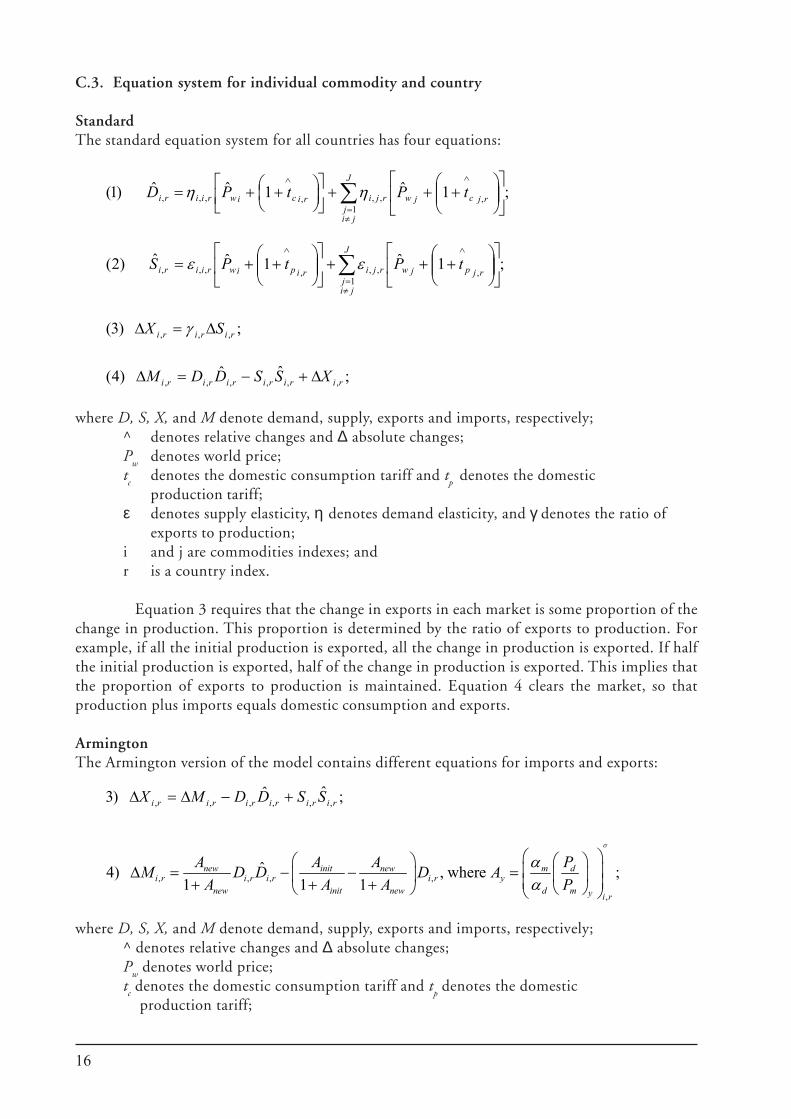
C.3. Equation system for individual commodity and country

StandardThe standard equation system for all countries has four equations:

;1ˆ1ˆˆ)1(1

,,,,,,, ∑≠=

∧∧

+++

++=

J

jij

rjcjwrjiriciwriiri tPtPD ηη

;1ˆ1ˆˆ)2(1

,,,,,,, ∑≠=

∧∧

+++

++=

J

jij

rjpjwrjiripiwriiri tPtPS εε

;)3( ,,, ririri SX ∆=∆ γ

;ˆˆ)4( ,,,,,, riririririri XSSDDM ∆+−=∆

where D, S, X, and M denote demand, supply, exports and imports, respectively;^ denotes relative changes and ∆ absolute changes;P

wdenotes world price;

tc

denotes the domestic consumption tariff and tp denotes the domestic

production tariff;ε denotes supply elasticity, η denotes demand elasticity, and γ denotes the ratio of

exports to production;i and j are commodities indexes; andr is a country index.

Equation 3 requires that the change in exports in each market is some proportion of thechange in production. This proportion is determined by the ratio of exports to production. Forexample, if all the initial production is exported, all the change in production is exported. If halfthe initial production is exported, half of the change in production is exported. This implies thatthe proportion of exports to production is maintained. Equation 4 clears the market, so thatproduction plus imports equals domestic consumption and exports.

ArmingtonThe Armington version of the model contains different equations for imports and exports:

;ˆˆ)3 ,,,,,, riririririri SSDDMX +−∆=∆

, , , ,

,

ˆ4) , where ;1 1 1

new init new m di r i r i r i r y

new init new d m y i r

A A A PM D D D AA A A P

σ

αα

∆ = − − = + + +

where D, S, X, and M denote demand, supply, exports and imports, respectively;^ denotes relative changes and ∆ absolute changes;P

w denotes world price;

tc denotes the domestic consumption tariff and t

p denotes the domestic

production tariff;

17

ε denotes supply elasticity, η denotes demand elasticity, and γ denotes the ratio of ex-ports to production;

i and j are commodities indexes;r is a country index;(P

d/P

m)

y=(P

w(1+t

d)/(P

w(1+t

m))

y ,where y=init indicates initial values and

y=new indicates values after the policy changes;σ denotes the Armington elasticity between imports and domesticallyproduced goods.

Equation 4 requires that the relation of imports and domestic supply is determined bythe price ratio of domestic supply and imports:

m d

d m

PMD M P

σαα

= −

Equation 3 clears the market, so that production plus imports equals domesticconsumption and exports.

The default value for the elasticity is 2.2, although for homegeneous goods there may bea sound argument for increasing this value.

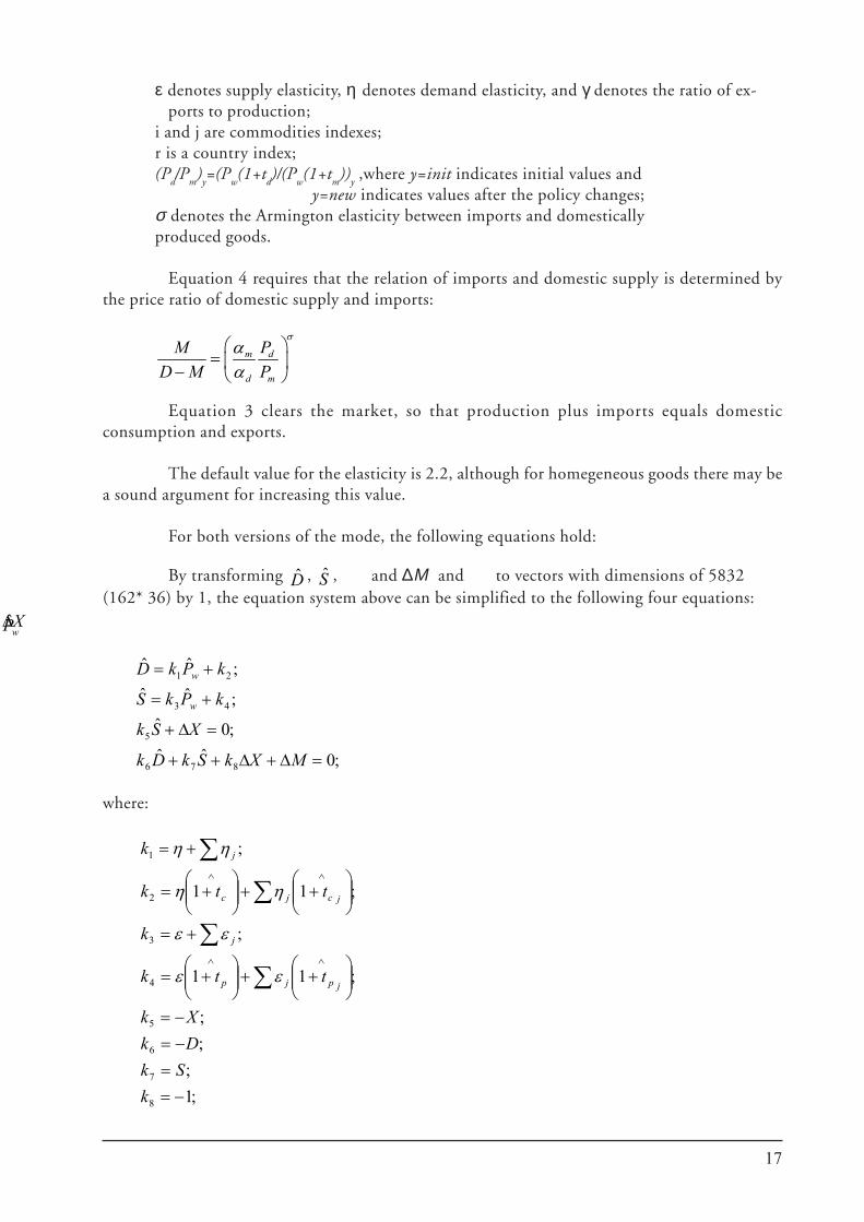
For both versions of the mode, the following equations hold:

By transforming D , S ,

X∆

and ∆Μ and

wP

to vectors with dimensions of 5832(162* 36) by 1, the equation system above can be simplified to the following four equations:

;0ˆˆ;0ˆ;ˆˆ;ˆˆ

876

5

43

21

=∆+∆++

=∆+

+=

+=

MXkSkDk

XSk

kPkS

kPkD

w

w

where:

;1;

;;

;11

;

;11

;

8

7

6

5

4

3

2

1

−==−=−=

++

+=

+=

++

+=

+=

∑

∑

∑

∑

∧∧

∧∧

kSk

DkXk

ttk

k

ttk

k

jpjp

j

jcjc

j

εε

εε

ηη

ηη

18

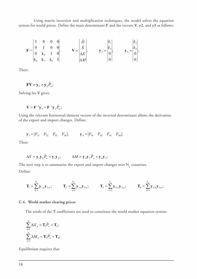
Using matrix inversion and multiplication techniques, the model solves the equationsystem for world prices. Define the main determinant F and the vectors V, y2, and y3 as follows:

;

00

;

00

;ˆˆ

;

Ikk0Ik000I0000I

= 4

2

33

1

2

876

5

kk

kk

MXSD

k

==

∆∆

= yyVF

Then:

;ˆ23 wPyyFV +=

Solving for V gives:

;ˆ2

13

1wPyFyFV −− +=

Using the relevant horizontal element vectors of the inverted determinant allows the derivationof the export and import changes. Define:

;; 444342414343332311 FFFFFFFF == yy

Then:

;ˆ;ˆ34243121 yyyyyyyy +=∆+=∆ ww PMPX

The next step is to summarize the export and import changes over Np countries.

Define:

∑∑∑∑====

====pppp N

nnn

N

nnn

N

nnn

N

nnn

1,3,44

1,2,43

1,3,12

1,2,11 ;;;; yyTyyTyyTyyT

C.4. World market clearing prices

The totals of the T coefficients are used to constitute the world market equation system:

∑

∑

=

=

+=∆

+=∆

N

nwn

N

nwn

PM

PX

143

121

;ˆ

;ˆ

TT

TT

Equilibrium requires that

19

;0)(1

=∆−∆∑=

N

nnn MX

i.e. the change in world excess supply is zero. This implies that

0)(ˆ)( 4231 =−+− TTTT wP.

Note that T1 and T

3 are square commodity matrices and that all other variables are commodity

vectors. Solving for the world market price change gives:

);()(ˆ42

131 TTTT −−−= −

wP

The absolute world market price change is:

;ˆwww PPP =∆

Once the world price changes are derived these changes can then be inserted into equations (1) to(4) to get the volume responses.

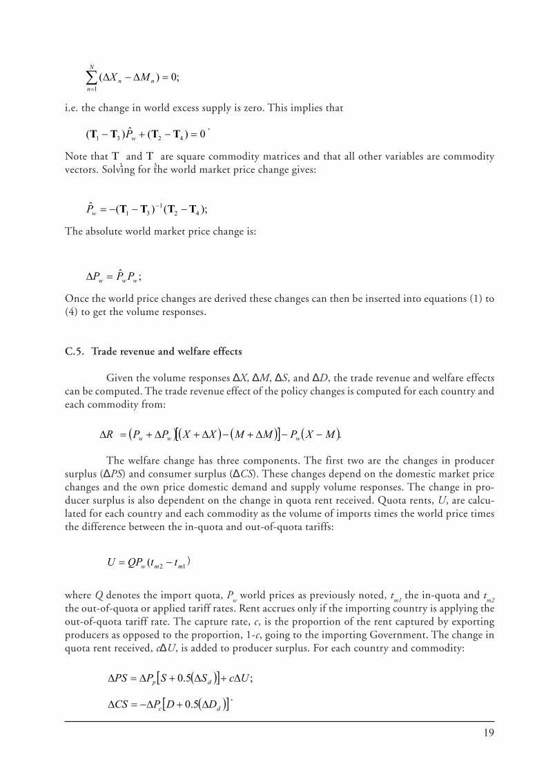
C.5. Trade revenue and welfare effects

Given the volume responses ∆X, ∆M, ∆S, and ∆D, the trade revenue and welfare effectscan be computed. The trade revenue effect of the policy changes is computed for each country andeach commodity from:

( ) ( ) ( )[ ] ( ).MXPMMXXPPR www −−∆+−∆+∆+=∆

The welfare change has three components. The first two are the changes in producersurplus (∆PS) and consumer surplus (∆CS). These changes depend on the domestic market pricechanges and the own price domestic demand and supply volume responses. The change in pro-ducer surplus is also dependent on the change in quota rent received. Quota rents, U, are calcu-lated for each country and each commodity as the volume of imports times the world price timesthe difference between the in-quota and out-of-quota tariffs:

12( mmw ttQPU −= )

where Q denotes the import quota, Pw world prices as previously noted, t

m1 the in-quota and t

m2

the out-of-quota or applied tariff rates. Rent accrues only if the importing country is applying theout-of-quota tariff rate. The capture rate, c, is the proportion of the rent captured by exportingproducers as opposed to the proportion, 1-c, going to the importing Government. The change inquota rent received, c∆U, is added to producer surplus. For each country and commodity:

( )[ ] ;5.0 UcSSPPS dp ∆+∆+∆=∆

( )[ ]dc DDPCS ∆+∆−=∆ 5.0.

20

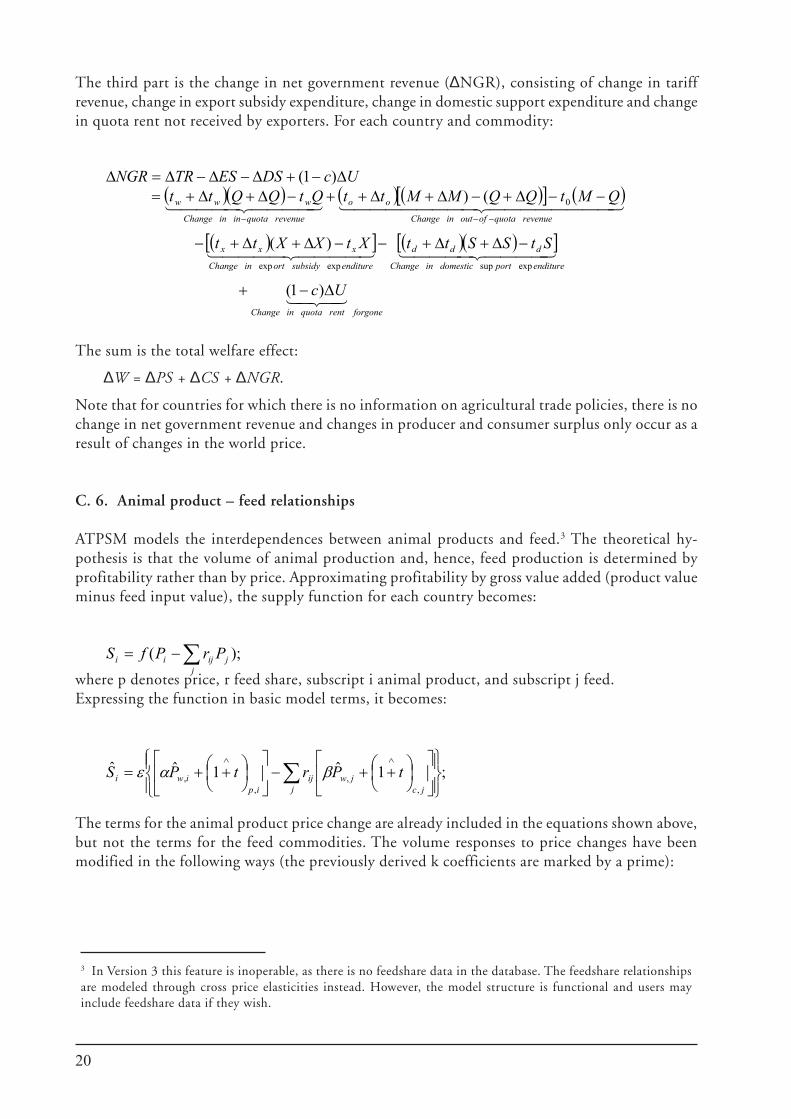
The third part is the change in net government revenue (∆NGR), consisting of change in tariffrevenue, change in export subsidy expenditure, change in domestic support expenditure and changein quota rent not received by exporters. For each country and commodity:

( )( ) ( ) ( )[ ] ( )

( )[ ] ( )( )[ ]

43421

4444 34444 214444 34444 21

44444444 344444444 214444 34444 21

forgonerentquotainChange

enditureportdomesticinChange

ddd

endituresubsidyortinChange

xxx

revenuequotaofoutinChange

oo

revenuequotaininChange

www

Uc

StSSttXtXXtt

QMtQQMMttQtQQttUcDSESTRNGR

∆−+

−∆+∆+−−∆+∆+−

−−∆+−∆+∆++−∆+∆+=∆−+∆−∆−∆=∆

−−−

)1(

)(

())1(

expsupexpexp

0

The sum is the total welfare effect:

∆W = ∆PS + ∆CS + ∆NGR.

Note that for countries for which there is no information on agricultural trade policies, there is nochange in net government revenue and changes in producer and consumer surplus only occur as aresult of changes in the world price.

C. 6. Animal product – feed relationships

ATPSM models the interdependences between animal products and feed.3 The theoretical hy-pothesis is that the volume of animal production and, hence, feed production is determined byprofitability rather than by price. Approximating profitability by gross value added (product valueminus feed input value), the supply function for each country becomes:

∑−=j

jijii PrPS );(fwhere p denotes price, r feed share, subscript i animal product, and subscript j feed.Expressing the function in basic model terms, it becomes:

;1ˆ1ˆˆ,

,,

,

++−

++= ∑

∧∧

j jcjwij

ipiwi tPrtPS βαε

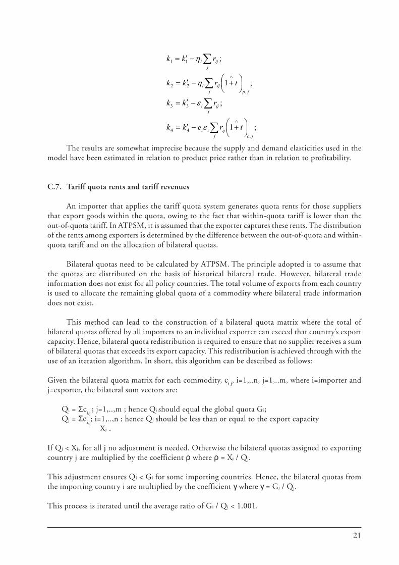
The terms for the animal product price change are already included in the equations shown above,but not the terms for the feed commodities. The volume responses to price changes have beenmodified in the following ways (the previously derived k coefficients are marked by a prime):

3 In Version 3 this feature is inoperable, as there is no feedshare data in the database. The feedshare relationshipsare modeled through cross price elasticities instead. However, the model structure is functional and users mayinclude feedshare data if they wish.

21

∑

∑

∑

∑

+−′=

−′=

+−′=

−′=

∧

∧

j jcijii

jiji

jpjiji

jiji

trekk

rkk

trkk

rkk

;1

;

;1

;

,44

33

,22

11

ε

ε

η

η

The results are somewhat imprecise because the supply and demand elasticities used in themodel have been estimated in relation to product price rather than in relation to profitability.

C.7. Tariff quota rents and tariff revenues

An importer that applies the tariff quota system generates quota rents for those suppliersthat export goods within the quota, owing to the fact that within-quota tariff is lower than theout-of-quota tariff. In ATPSM, it is assumed that the exporter captures these rents. The distributionof the rents among exporters is determined by the difference between the out-of-quota and within-quota tariff and on the allocation of bilateral quotas.

Bilateral quotas need to be calculated by ATPSM. The principle adopted is to assume thatthe quotas are distributed on the basis of historical bilateral trade. However, bilateral tradeinformation does not exist for all policy countries. The total volume of exports from each countryis used to allocate the remaining global quota of a commodity where bilateral trade informationdoes not exist.

This method can lead to the construction of a bilateral quota matrix where the total ofbilateral quotas offered by all importers to an individual exporter can exceed that country’s exportcapacity. Hence, bilateral quota redistribution is required to ensure that no supplier receives a sumof bilateral quotas that exceeds its export capacity. This redistribution is achieved through with theuse of an iteration algorithm. In short, this algorithm can be described as follows:

Given the bilateral quota matrix for each commodity, ci,j, i=1,..n, j=1,..m, where i=importer andj=exporter, the bilateral sum vectors are:

Qi = Σci,j ; j=1,..,m ; hence Qi

should equal the global quota Gi;

Qj = Σci,j; i=1,..,n ; hence Qj should be less than or equal to the export capacity Xj .

If Qj < Xj, for all j no adjustment is needed. Otherwise the bilateral quotas assigned to exportingcountry j are multiplied by the coefficient ρ where ρ = Xj / Qj.

This adjustment ensures Qi < Gi for some importing countries. Hence, the bilateral quotas fromthe importing country i are multiplied by the coefficient γ where γ = Gj / Qj.

This process is iterated until the average ratio of Gi / Qi < 1.001.

22

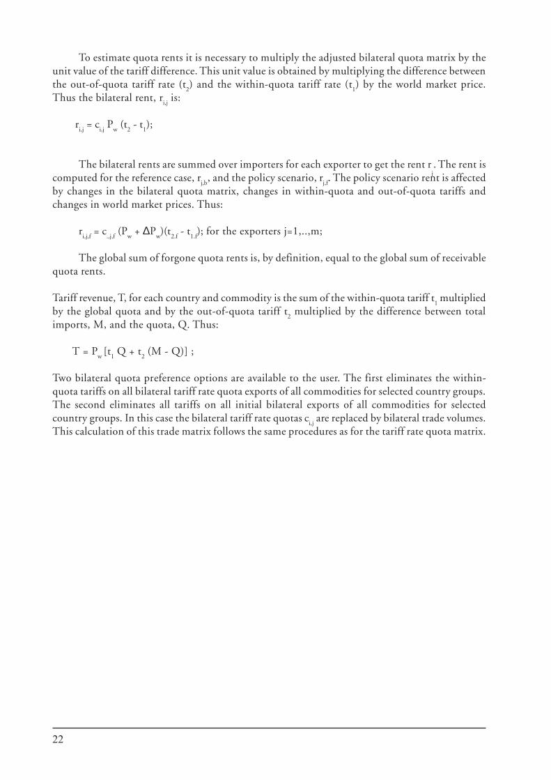
To estimate quota rents it is necessary to multiply the adjusted bilateral quota matrix by theunit value of the tariff difference. This unit value is obtained by multiplying the difference betweenthe out-of-quota tariff rate (t

2) and the within-quota tariff rate (t

1) by the world market price.

Thus the bilateral rent, ri,j is:

ri,j = c

i,j P

w (t

2 - t

1);

The bilateral rents are summed over importers for each exporter to get the rent rj. The rent is

computed for the reference case, rj,b

, and the policy scenario, rj,f. The policy scenario rent is affected

by changes in the bilateral quota matrix, changes in within-quota and out-of-quota tariffs andchanges in world market prices. Thus:

ri,j,f

= c.,j,f

(Pw + ∆P

w)(t

2.f - t

1.f); for the exporters j=1,..,m;

The global sum of forgone quota rents is, by definition, equal to the global sum of receivablequota rents.

Tariff revenue, T, for each country and commodity is the sum of the within-quota tariff t1 multiplied

by the global quota and by the out-of-quota tariff t2 multiplied by the difference between total

imports, M, and the quota, Q. Thus:

T = Pw

[t

1 Q + t

2 (M - Q)] ;

Two bilateral quota preference options are available to the user. The first eliminates the within-quota tariffs on all bilateral tariff rate quota exports of all commodities for selected country groups.The second eliminates all tariffs on all initial bilateral exports of all commodities for selectedcountry groups. In this case the bilateral tariff rate quotas c

i,j are replaced by bilateral trade volumes.

This calculation of this trade matrix follows the same procedures as for the tariff rate quota matrix.

23

All initial data are stored in the Access database file atpsm.mdb. It is possible to run ATPSMwithout having Microsoft Access, but it is not possible to change the initial data without thissoftware.

D.1. Country list

The total number of countries in the model is 162 (or, counting the EU 15 members, 176countries). One country is labelled Rest of World, essentially a residual to balance the initial data-base. The country names and codes can be found in Appendix I. The trade policy data require-ments are discussed in the relevant sections below.

D.2. Prices and volumes

The world market prices have been developed using several sources (International FinancialStatistics, FAO Trade Yearbook and UNCTAD price statistics), extending the period covered from1999 to 2001.

The volumes of trade and production have been obtained from the FAO supply utilizationaccounts. Consumption is obtained by adding imports and production and subtracting exports –so-called apparent consumption. This concept does not take into account movements in and outof stocks. Sometimes, owing to incompatibility between production and trade accounts, the ap-parent consumption can equate to a negative number. In such a case production is increased toensure that consumption is non-negative.

As the commodity specification in the supply utilization accounts is more detailed than theone used in the ATPSM, the volumes were aggregated applying appropriate conversion factors. Tostabilize the data for annual variations in yield, a three-year average of volumes from 1999 to 2001was estimated.

D.3. Bilateral trade flows

As bilateral tariff quotas are incompletely specified in the notifications to the WTO, infor-mation about bilateral trade flows becomes a necessary means for distributing the global tariffquotas among exporters. The procedure implies that the tariff quotas tend to be distributed totraditional suppliers.

The database of the UNCTAD trade deflator system is used as a data source. First, intra-EUtrade is eliminated, as the EU countries are treated as one region in the model. As the trade flowsare reported at HS line level, the next step is to sum up the HS flows to the level of the ATPSMcommodity groups. The resulting bilateral trade flows are listed in the sub-file “TRADE” in thefile atpsm.mdb.

PART D: THE ATPSM DATABASE

24

D.4. Tariffs and tariff quotas

All import trade barriers (out-of-quota and within-quota tariff rates and tariff rate quotas)are derived using information from the Agricultural Market Access Database (AMAD). AMAD ispublicly accessible from the website www.amad.org. It is maintained by the OECD, and a numberof other organizations, including FAO, UNCTAD, the US Department of Agriculture, AgricultureCanada and the EU Agricultural Directorate, contribute to its development. Most of the data inAMAD come from WTO schedules and notifications. However, the applied rates are obtainedfrom the UNCTAD TRAINS database.

There are three problems to address in converting AMAD data to a format suitable for use inATPSM:

1. For some countries and many tariff lines, the tariffs are specific or mixed;

2. The tariffs in the notifications provided by countries to WTO are specified by HS line;

3. For several countries, the implementation period for tariff cuts prescribed in the Agree-ment on Agriculture goes beyond the year 2000.

As mentioned previously, in ATPSM all tariffs must be expressed as a percentage of theworld market price. The method for converting specific and mixed tariffs into ad-valorem equivalentsis detailed in Appendix II.

The AMAD files containing the within-quota tariff information also contain tariff quotadata. Therefore, the quotas in these files are summed to ATPSM commodity group levelsimultaneously with the weighted (or simple) aggregation of the within-quota tariffs. The quotasums represent the global tariff quotas. The main difficulty encountered in this aggregation is thattariff quotas in several cases cover commodity groups both inside and outside the ATPSMframework. In such instances the quota is allocated to the commodity group (inside or outsideATPSM) with the most imports.

The data are listed in three ATPSM sub-files, “INQUOTAS”, “OUTQUOTA” and“AppliedTariffRates”.

D.5. Export subsidies

The data on export subsidies and quotas are based on government notifications to WTO.They can be found in the atpsm.mdb subfileExportSubsidies.

D.6. Domestic support

The Uruguay Round Agreement on Agriculture calls for reductions in production-distorting(amber box) domestic support. However, it is not clear to what extent differing forms of domesticsupport distort production and trade. Direct income support and payments to factors of productionhave less effect on output than payments on output. In addition, in some instances administeredprices appear to be providing domestic support, but such policies actually rely on border measuresfor their effect. Double counting can occur where domestic support is conflated with borderprotection. (See de Gorter, Ingco and Ignacio (2004, p. 122) for elaboration of this point.) TheATPSM database attempts to avoid this. The support has been converted into tariff ad-valorem

25

equivalents through dividing unit support by the world market price. The domestic support isfound in the subfile “DomesticSupport”.

This approach implies low rates of domestic support for the European Union and the UnitedStates. The production-limiting (blue box) items in EU domestic support are debatable, as atpresent they are accompanied by production limits. The justification for excluding blue box supportis that it is difficult to assess whether the production limits offset the additional support. Greenbox support is exempt from reduction commitments. The impact of amber, blue and green boxsupport on production is a grey area, the subject of an ongoing decoupling debate.

D.7. Price elasticities

To calculate price elasticities for the ATPSM the supply and demand elasticities available inthe FAO databases was used. The FAO database on price elasticities covers direct and cross-priceelasticities for domestic demand, and area supply and yield of major agricultural commodities.

For the purpose of the ATPSM, the area and yield elasticities from FAO are used to estimatea supply elasticity. Given that supply (S) is the product of area (A) and yield (Y),

S = A Y

the supply elasticity is simply the sum of the area and yield elasticities. Taking the logarithm of theequation:

log S = log A + log Y;

then, dividing all the three elements by log P, it follows that:

es = ea + ey

There are a number of countries represented in ATPSM for which no FAO estimate ofsupply or demand elasticity exists. In these instances, the elasticities are assumed to be the same asthose for a geographically close proxy region. The price elasticities are listed in the sub-file“Elasticities”.

26

Abbott, P. and Morse, B. A. (1999). TRQ implementation in developing countries, paper pre-sented at the Conference on Agriculture and the New Trade Agenda in the WTO 2000Negotiations, October 1999, Geneva, World Bank and World Trade Organization.

AMAD database http://www.amad.org.

De Gorter, H., Ingco, M. and Ignacio, L. (2004). ‘Domestic support: economics and policyinstruments’, in Ingco, M. and Nash, J. (eds) Agriculture and the WTO: creating a TradingSystem for Development, World Bank, Washington, D.C.

De Gorter, H. and Sheldon, I., eds. (2000). Issues in reforming tariff-rate import quotas in theagreement on agriculture in the WTO, Commissioned Paper No. 13, International Agricul-tural Trade Research Consortium.

FAOSTAT database http://apps.fao.org.

Skully, D.W. (2001). The economics of TRQ administration, Technical Bulletin No. 1893.Washington, DC, Economic Research Service, US Department of Agriculture.

UNCTAD (1990). Agricultural trade liberalization in the Uruguay Round: Implications fordeveloping countries (UNCTAD/ITP/48), Geneva.

UNCTAD TRAINS database http://www.unctad.org/trains/index.htm

REFERENCES

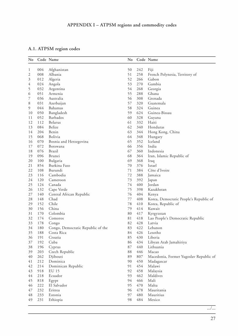
27

1 004 Afghanistan2 008 Albania3 012 Algeria4 024 Angola5 032 Argentina6 051 Armenia7 036 Australia8 031 Azerbaijan9 044 Bahamas10 050 Bangladesh11 052 Barbados12 112 Belarus13 084 Belize14 204 Benin15 068 Bolivia16 070 Bosnia and Herzegovina17 072 Botswana18 076 Brazil19 096 Brunei20 100 Bulgaria21 854 Burkina Faso22 108 Burundi23 116 Cambodia24 120 Cameroon25 124 Canada26 132 Cape Verde27 140 Central African Republic28 148 Chad29 152 Chile30 156 China31 170 Colombia32 174 Comoros33 178 Congo34 180 Congo, Democratic Republic of the35 188 Costa Rica36 191 Croatia37 192 Cuba38 196 Cyprus39 203 Czech Republic40 262 Djibouti41 212 Dominica42 214 Dominican Republic43 918 EU 1544 218 Ecuador45 818 Egypt46 222 El Salvador47 232 Eritrea48 233 Estonia49 231 Ethiopia

APPENDIX I – ATPSM regions and commodity codes

50 242 Fiji51 258 French Polynesia, Territory of52 266 Gabon53 270 Gambia54 268 Georgia55 288 Ghana56 308 Grenada57 320 Guatemala58 324 Guinea59 624 Guinea-Bissau60 328 Guyana61 332 Haiti62 340 Honduras63 344 Hong Kong, China64 348 Hungary65 352 Iceland66 356 India67 360 Indonesia68 364 Iran, Islamic Republic of69 368 Iraq70 376 Israel71 384 Côte d’Ivoire72 388 Jamaica73 392 Japan74 400 Jordan75 398 Kazakhstan76 404 Kenya77 408 Korea, Democratic People‘s Republic of78 410 Korea, Republic of79 414 Kuwait80 417 Kyrgyzstan81 418 Lao People‘s Democratic Republic82 428 Latvia83 422 Lebanon84 426 Lesotho85 430 Liberia86 434 Libyan Arab Jamahiriya87 440 Lithuania88 446 Macao89 807 Macedonia, Former Yugoslav Republic of90 450 Madagascar91 454 Malawi92 458 Malaysia93 462 Maldives94 466 Mali95 470 Malta96 478 Mauritania97 480 Mauritius98 484 Mexico

.../...

A.1. ATPSM region codes

No Code Name No Code Name

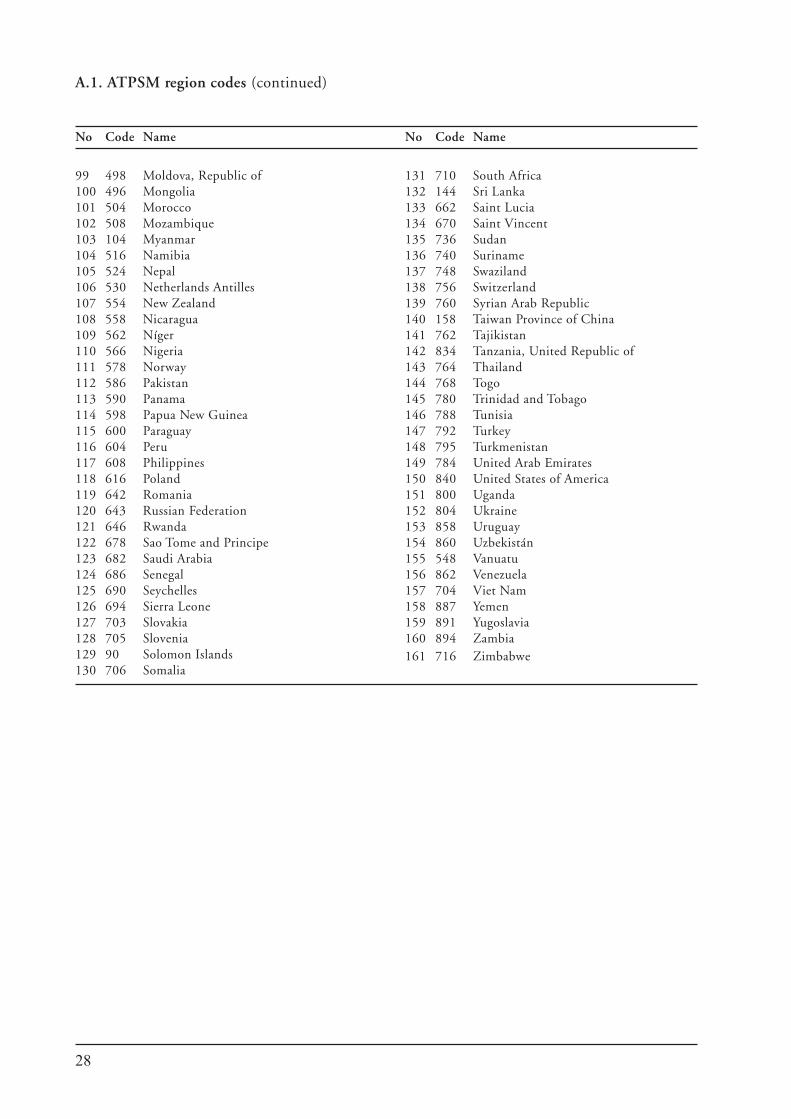
28

99 498 Moldova, Republic of100 496 Mongolia101 504 Morocco102 508 Mozambique103 104 Myanmar104 516 Namibia105 524 Nepal106 530 Netherlands Antilles107 554 New Zealand108 558 Nicaragua109 562 Níger110 566 Nigeria111 578 Norway112 586 Pakistan113 590 Panama114 598 Papua New Guinea115 600 Paraguay116 604 Peru117 608 Philippines118 616 Poland119 642 Romania120 643 Russian Federation121 646 Rwanda122 678 Sao Tome and Principe123 682 Saudi Arabia124 686 Senegal125 690 Seychelles126 694 Sierra Leone127 703 Slovakia128 705 Slovenia129 90 Solomon Islands130 706 Somalia

131 710 South Africa132 144 Sri Lanka133 662 Saint Lucia134 670 Saint Vincent135 736 Sudan136 740 Suriname137 748 Swaziland138 756 Switzerland139 760 Syrian Arab Republic140 158 Taiwan Province of China141 762 Tajikistan142 834 Tanzania, United Republic of143 764 Thailand144 768 Togo145 780 Trinidad and Tobago146 788 Tunisia147 792 Turkey148 795 Turkmenistan149 784 United Arab Emirates150 840 United States of America151 800 Uganda152 804 Ukraine153 858 Uruguay154 860 Uzbekistán155 548 Vanuatu156 862 Venezuela157 704 Viet Nam158 887 Yemen159 891 Yugoslavia160 894 Zambia161 716 Zimbabwe

A.1. ATPSM region codes (continued)

No Code Name No Code Name

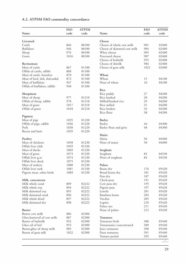
29

LivestockCattle 866 00100Buffaloes 946 00100Sheep 976 00100Goats 1016 00100

BovinemeatMeat of cattle 867 01100Offals of cattle, edible 868 01100Meat of cattle, boneless 870 01100Meat of beef, drd, sltd,smkd 872 01100Meat of buffaloes 947 01100Offals of buffaloes, edible 948 01100

SheepmeatMeat of sheep 977 01210Offals of sheep, edible 978 01210Meat of goats 1017 01210Offals of goats 1018 01210

PigmeatMeat of pigs 1035 01220Offals of pigs, edible 1036 01220Pork 1038 01220Bacon and ham 1039 01220

PoultryMeat of chickens 1058 01230Offals liver chik 1059 01230Meat of ducks 1069 01230Meat of geese 1073 01230Offals liver g.se 1074 01230Offals liver duck 1075 01230Meat of turkeys 1080 01230Offals liver turk 1081 01230Pigeon meat, other birds 1089 01230

Milk, concentrateMilk whole cond 889 02222Milk whole evp 894 02222Milk skimmed evp 895 02222Milk skimmed cond 896 02222Milk whole dried 897 02222Milk skimmed dry 898 02222

ButterButter cow milk 886 02300Ghee,butteroil of cow milk 887 02300Butter of bufmilk 952 02300Ghee oil of buf 953 02300Butter,ghee of sheep milk 983 02300Butter of goat mlk 1022 02300

CheeseCheese of whole cow milk 901 02400Cheese of skimmed cow milk 904 02400Whey cheese 905 02400Processed cheese 907 02400Cheese of bufmilk 955 02400Cheese of shmilk 984 02400Cheese of goat mlk 1021 02400

WheatWheat 15 04100Flour of wheat 16 04100

RiceRice paddy 27 04200Rice husked 28 04200Milled/husked rice 29 04200Rice milled 31 04200Rice broken 32 04200Rice flour 38 04200

BarleyBarley 44 04300Barley flour and grits 48 04300

MaizeMaize 56 04400Flour of maize 58 04400

SorghumSorghum 83 04530Flour of sorghum 84 04530

PulsesBeans dry 176 05420Broad beans dry 181 05420Peas dry 187 05420Chick-peas 191 05420Cow peas dry 195 05420Pigeon peas 197 05420Lentils 201 05420Bambara beans 203 05420Vetches 205 05420Lupins 210 05420Pulses nes 211 05420Flour of pulses 212 05420

TomatoesTomatoes fresh 388 05440Tomatojuice concentrated 389 05440Juice tomatoes 390 05440Paste tomatoes 391 05440Tomato peeled 392 05440

A.2. ATPSM FAO commodity concordance

FAO ATPSMName code code

FAO ATPSMName code code

.../...

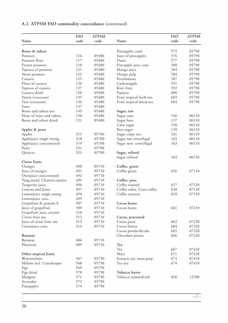
30

Roots & tubersPotatoes 116 05480Potatoes flour 117 05480Frozen potatoes 118 05480Tapioca of potatoes 121 05480Sweet potatoes 122 05480Cassava 125 05480Flour of cassava 126 05480Tapioca of cassava 127 05480Cassava dried 128 05480Yautia (cocoyam) 135 05480Taro (cocoyam) 136 05480Yams 137 05480Roots and tubers nes 149 05480Flour of roots and tubers 150 05480Roots and tubers dried 151 05480

Apples & pearsApples 515 05700Applejuice single streng 518 05700Applejuice concentrated 519 05700Pears 521 05700Quinces 523 05700

Citrus fruitsOranges 490 05710Juice of oranges 491 05710Oranjuice concentrated 492 05710Tang.mand. Clement.satsma 495 05710Tangerine juice 496 05710Lemons and limes 497 05710Lemonjuice single-streng 498 05710Lemonjuice conc. 499 05710Grapefruit & pomelo 0 507 05710Juice of grapefruit 509 05710Grapefruit juice cocentr 510 05710Citrus fruit nes 512 05710Juice of citrus fruit nes 513 05710Citrusjuice conc. 514 05710

BananasBananas 486 05710Plantains 489 05710

Other tropical fruitsWatermelons 567 05790Melons incl. Cantaloupes 568 05790Figs 569 05790Figs dried 570 05790Mangoes 571 05790Avocados 572 05790Pineapples 574 05790

A.2. ATPSM FAO commodity concordance (continued)

FAO ATPSMName code code

FAO ATPSMName code code

Pineapples cand 575 05790Juice of pineapples 576 05790Dates 577 05790Pineapple juice conc 580 05790Mango juice 583 05790Mango pulp 584 05790Persimmons 587 05790Cashewapple 591 05790Kiwi fruit 592 05790Papayas 600 05790Fruit tropical fresh nes 603 05790Fruit tropical dried nes 604 05790

Sugar, rawSugar cane 156 06110Sugar beet 157 06110Cane sugar 158 06110Beet sugar 159 06110Sugar crops nes 161 06110Sugar raw centrifugal 162 06110Sugar non- centrifugal 163 06110

Sugar, refinedSugar refined 164 06120

Coffee, greenCoffee green 656 07110

Coffee, proc.Coffee roasted 657 07120Coffee subst. Cont.coffee 658 07120Coffee extracts 659 07120

Cocoa beansCocoa beans 661 07210

Cocoa, processedCocoa paste 662 07220Cocoa butter 664 07220Cocoa powder&cake 665 07220Chocolate prsnes 666 07220

TeaTea 667 07410Mate 671 07410Extracts tea, mate,prep. 672 07410Tea nes 674 07410

Tobacco leavesTobacco unmanfcted 826 12100

.../...

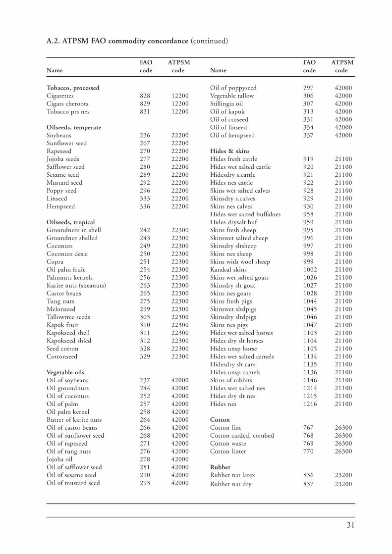
31

Tobacco, processedCigarettes 828 12200Cigars cheroots 829 12200Tobacco prs nes 831 12200

Oilseeds, temperateSoybeans 236 22200Sunflower seed 267 22200Rapeseed 270 22200Jojoba seeds 277 22200Safflower seed 280 22200Sesame seed 289 22200Mustard seed 292 22200Poppy seed 296 22200Linseed 333 22200Hempseed 336 22200

Oilseeds, tropicalGroundnuts in shell 242 22300Groundnut shelled 243 22300Coconuts 249 22300Coconuts desic 250 22300Copra 251 22300Oil palm fruit 254 22300Palmnuts kernels 256 22300Karite nuts (sheanuts) 263 22300Castor beans 265 22300Tung nuts 275 22300Melonseed 299 22300Tallowtree seeds 305 22300Kapok fruit 310 22300Kapokseed shell 311 22300Kapokseed shled 312 22300Seed cotton 328 22300Cottonseed 329 22300

Vegetable oilsOil of soybeans 237 42000Oil groundnuts 244 42000Oil of coconuts 252 42000Oil of palm 257 42000Oil palm kernel 258 42000Butter of karite nuts 264 42000Oil of castor beans 266 42000Oil of sunflower seed 268 42000Oil of rapeseed 271 42000Oil of tung nuts 276 42000Jojoba oil 278 42000Oil of safflower seed 281 42000Oil of sesame seed 290 42000Oil of mustard seed 293 42000

Oil of poppyseed 297 42000Vegetable tallow 306 42000Stillingia oil 307 42000Oil of kapok 313 42000Oil of ctnseed 331 42000Oil of linseed 334 42000Oil of hempseed 337 42000

Hides & skinsHides fresh cattle 919 21100Hides wet salted cattle 920 21100Hidesdry s.cattle 921 21100Hides nes cattle 922 21100Skins wet salted calves 928 21100Skinsdry s.calves 929 21100Skins nes calves 930 21100Hides wet salted buffaloes 958 21100Hides drysalt buf 959 21100Skins fresh sheep 995 21100Skinswet salted sheep 996 21100Skinsdry sltsheep 997 21100Skins nes sheep 998 21100Skins with wool sheep 999 21100Karakul skins 1002 21100Skins wet salted goats 1026 21100Skinsdry slt goat 1027 21100Skins nes goats 1028 21100Skins fresh pigs 1044 21100Skinswet sltdpigs 1045 21100Skinsdry sltdpigs 1046 21100Skins nes pigs 1047 21100Hides wet salted horses 1103 21100Hides dry slt horses 1104 21100Hides unsp horse 1105 21100Hides wet salted camels 1134 21100Hidesdry slt cam 1135 21100Hides unsp camels 1136 21100Skins of rabbits 1146 21100Hides wet salted nes 1214 21100Hides dry slt nes 1215 21100Hides nes 1216 21100

CottonCotton lint 767 26300Cotton carded, combed 768 26300Cotton waste 769 26300Cotton linter 770 26300

RubberRubber nat latex 836 23200Rubber nat dry 837 23200

A.2. ATPSM FAO commodity concordance (continued)

FAO ATPSMName code code

FAO ATPSMName code code

32

33

UNCTAD Study Series on

POLICY ISSUES IN INTERNATIONAL TRADEAND COMMODITIES

No. 1 Erich Supper, Is there effectively a level playing field for developing countryexports?, 2001, 138 p. Sales No. E.00.II.D.22.

No. 2 Arvind Panagariya, E-commerce, WTO and developing countries, 2000, 24 p.Sales No. E.00.II.D.23.

No. 3 Joseph Francois, Assessing the results of general equilibrium studies of multi-lateral trade negotiations, 2000, 26 p. Sales No. E.00.II.D.24.

No. 4 John Whalley, What can the developing countries infer from the UruguayRound models for future negotiations?, 2000, 29 p. Sales No. E.00.II.D.25.

No. 5 Susan Teltscher, Tariffs, taxes and electronic commerce: Revenue implicationsfor developing countries, 2000, 57 p. Sales No. E.00.II.D.36.

No. 6 Bijit Bora, Peter J. Lloyd, Mari Pangestu, Industrial policy and the WTO, 2000,47 p. Sales No. E.00.II.D.26.

No. 7 Emilio J. Medina-Smith, Is the export-led growth hypothesis valid for develop-ing countries? A case study of Costa Rica, 2001, 49 p. Sales No. E.01.II.D.8.

No. 8 Christopher Findlay, Service sector reform and development strategies: Issuesand research priorities, 2001, 24 p. Sales No. E.01.II.D.7.

No. 9 Inge Nora Neufeld, Anti-dumping and countervailing procedures – Use orabuse? Implications for developing countries, 2001, 33 p. Sales No. E.01.II.D.6.

No. 10 Robert Scollay, Regional trade agreements and developing countries: The caseof the Pacific Islands’ proposed free trade agreement, 2001, 45 p. Sales No.E.01.II.D.16.

No. 11 Robert Scollay and John Gilbert, An integrated approach to agricultural tradeand development issues: Exploring the welfare and distribution issues, 2001,43 p. Sales No. E.01.II.D.15.

No. 12 Marc Bacchetta and Bijit Bora, Post-Uruguay round market access barriersfor industrial products, 2001, 50 p. Sales No. E.01.II.D.23.

No. 13 Bijit Bora and Inge Nora Neufeld, Tariffs and the East Asian financial crisis,2001, 30 p. Sales No. E.01.II.D.27.

34

No. 14 Bijit Bora, Lucian Cernat, Alessandro Turrini, Duty and Quota-Free Access forLDCs: Further Evidence from CGE Modelling, 2002, 130 p. Sales No.E.01.II.D.22.

No. 15 Bijit Bora, John Gilbert, Robert Scollay, Assessing regional trading arrange-ments in the Asia-Pacific, 2001, 29 p. Sales No. E.01.II.D.21.

No. 16 Lucian Cernat, Assessing regional trade arrangements: Are South-South RTAsmore trade diverting?, 2001, 24 p. Sales No. E.01.II.D.32.

No. 17 Bijit Bora, Trade related investment measures and the WTO: 1995-2001, 2002.

No. 18 Bijit Bora, Aki Kuwahara, Sam Laird, Quantification of non-tariff measures,2002, 42 p. Sales No. E.02.II.D.8.

No. 19 Greg McGuire, Trade in services – Market access opportunities and the ben-efits of liberalization for developing economies, 2002, 45 p. Sales No. E.02.II.D.9.

No. 20 Alessandro Turrini, International trade and labour market performance: majorfindings and open questions, 2002, 30 p. Sales No. E.02.II.D.10.

No. 21 Lucian Cernat, Assessing south-south regional integration: same issues, manymetrics, 2003, 32 p. Sales No. E.02.II.D.11.

No. 22 Kym Anderson, Agriculture, trade reform and poverty reduction: implicationsfor Sub-Saharan Africa, 2004, Sales No. E.04.II.D.5.

No. 23 Ralf Peters and David Vanzetti, Shifting sands: searching for a compromise inthe WTO negotiations on agriculture, 2004, Sales No. E.04.II.D.4.

No. 24 Ralf Peters and David Vanzetti, User manual and handbook on agriculturaltrade policy simulation model (ATPSM), 2004, Sales No. E.04.II.D.3.

35

United Nations publications may be obtained from bookstores and distributors throughout the world.Please consult your bookstore or write to:

United Nations Publications

All orders from North America, Latin America, the Caribbean and Asia and the Pacific shouldbe sent to:

United Nations PublicationsRoom DC2-853, 2 UN PlazaNew York, NY 10017, USATelephone: (212) 963-8302, Toll Free 1-800-253-9646 (North America only)Fax: (212) 963-3489E-mail: publications@un.org

Customers in Europe, Africa and the Middle East should send their orders to:Section des Ventes et CommercialisationBureau E-4, CH-1211Geneva 10, SwitzerlandTelephone: 41 (22) 917-2613/2614Fax: 41 (22) 917-0027E-mail: unpubli@unog.ch

36

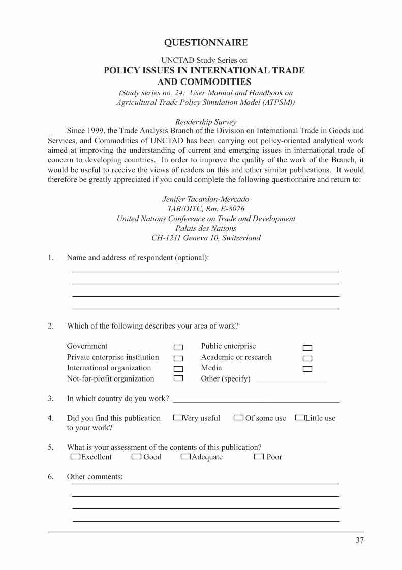
37

QUESTIONNAIRE

UNCTAD Study Series onPOLICY ISSUES IN INTERNATIONAL TRADE

AND COMMODITIES(Study series no. 24: User Manual and Handbook on

Agricultural Trade Policy Simulation Model (ATPSM))

Readership SurveySince 1999, the Trade Analysis Branch of the Division on International Trade in Goods and

Services, and Commodities of UNCTAD has been carrying out policy-oriented analytical workaimed at improving the understanding of current and emerging issues in international trade ofconcern to developing countries. In order to improve the quality of the work of the Branch, itwould be useful to receive the views of readers on this and other similar publications. It wouldtherefore be greatly appreciated if you could complete the following questionnaire and return to:

Jenifer Tacardon-MercadoTAB/DITC, Rm. E-8076

United Nations Conference on Trade and DevelopmentPalais des Nations

CH-1211 Geneva 10, Switzerland

1. Name and address of respondent (optional):

2. Which of the following describes your area of work?

Government Public enterprisePrivate enterprise institution Academic or researchInternational organization MediaNot-for-profit organization Other (specify) _________________

3. In which country do you work? _________________________________________

4. Did you find this publication Very useful Of some use Little useto your work?

5. What is your assessment of the contents of this publication? Excellent Good Adequate Poor

6. Other comments: