USER MANUAL

for

Low Cost Home Ownership

Version 7.24

Shelton Development Services Ltd

Redcroft House

Redcroft Walk

Cranleigh

Surrey GU6 8DS

Tel. 0845 678 9 876 Fax. 0845 076 3777

Email support@sdsproval.co.uk

2

Contents 1.0 Starting & Exiting SDS ProVal Page 3

1.1 Start SDS ProVal 3 1.2 Exit SDS ProVal 3

2.0 Open, Save & Close Appraisal Files 4 2.1 Start a New Appraisal 4 2.2 Open an Existing Appraisal 4 2.3 Save a New Appraisal 4 2.4 Save an Existing Appraisal as a New Version 4 2.5 Close an Appraisal 4 3.0 Navigation Controls 5 3.1 Screen Sizing 5 4.0 Setting and Applying Default Values 5

4.1 Personal Defaults 5 4.2 System Defaults 6 4.3 Dwelling Names & January 1999 Values 6 4.4 Defaults Validation Report 7 4.5 Updating an Existing Appraisal with New Default Values 7

5.0 Carrying out a Quick Appraisal 7 6.0 Carrying out a Full Appraisal 8

6.1 Entering Data 7 6.2 Memorandum Information 8 6.3 Scheme Header Details 8 6.4 Unit Details, Grant Index & On-Costs 9 6.5 Qualifying Scheme Cost 10 6.6 Scheme Cost Index 10 6.7 Grant 10 6.8 Analysis of On-Costs (excl. interest) 11 6.9 Scheme Timing 11 6.10 Comparison of On-Costs 13 6.11 Summary of Total Scheme Costs 14 6.12 Private Finance 14 6.13 Inflation & Rent Allowances 15 6.14 Cost Rent at Year 1 15 6.15 Set Rents for Long Term Cashflow 16 6.16 Cost to Purchaser & Affordability Ratios 17 6.17 Long Term Cashflow 18 6.18 Staircasing 21

7.0 Sensitivity Analysis 21 8.0 Benchmarks 22 9.0 Printing 23 10.0 Exporting Data 24 11.0 Help 24 Appendix 25 Creating Links & Entering User Defined Calculations 25 November 2011

3

Changes Incorporated Since The Last Manual

Compatibility with Excel 2003, 2007 and 2010 incorporated. Keyboard shortcuts added.

1.0 Starting & Exiting

Starting ProVal will amend the Excel operating environment and as a precaution the user should first close any other workbooks which may be open in Excel. Exiting will restore the Excel environment. An existing appraisal file cannot be opened in Excel as though it was an ordinary workbook because the necessary database and code files will not be present.

1.1 Start Double click on the desktop shortcut icon. Starting from the shortcut provided will open Excel and ensure ProVal system files are opened. ProVal appraisal files cannot be read properly in Excel on their own, therefore it is not possible to copy files onto another machine and open them in Excel.

1.2 Exit 1. Ensure any open appraisals have been closed. To check that all

appraisals have been closed, click the button View Opened Files.

2. To exit ProVal and restore the Microsoft Excel environment to its

normal position, click the button Exit ProVal.

4

2.0 Open, Save & Close Appraisal Files

2.1 Start a New Appraisal

1. From the Control Panel, click the button Start New.

2. Choose Low Cost Home Ownership Version 7xx from the modules listed in the dialog box and click OK button once. Refer to the Website for a list of the latest file versions.

2.2 Open an Existing Appraisal

1. From the Control Panel, click Open Existing File.

2. Select Appraisal File from the options listed. 3. Choose the appraisal file to be opened from the Open dialog box. Navigate to

the correct drive and folder as necessary. See also 4.1 for setting a preferred folder to open into.

2.3 Save a New Appraisal

1. Click Home Page

2. Click Save.

3. Check that the folder name which is shown in the Save As dialog box is correct. A default folder name can be set in Personal Defaults [see 4.1].

4. Enter or amend the file name as necessary.

5. Click the Save button to save the appraisal.

2.4 Save an Existing Appraisal as a New Version An appraisal can only be saved as a new version, after it has been saved for the first time. See 2.3 above.

1. Click Home Page

2. Click Save as New Version.

3. Verify the name of the new file and the folder in which it is to be saved.

4. Click Save.

5. Enter a password (twice) to protect the appraisal (i.e. make it Read-Only) as appropriate. Password protected files can still be opened and read, but cannot be amended unless the password is supplied. Ensure you keep a note of any passwords as these cannot be recovered by your supplier.

! Tip Amend the description of the Appraisal Version cell in the header section of the appraisal to describe the new version being saved. This data will be used to generate a new file name incorporating the version description.

2.5 Close an Appraisal

1. Click Home Page

2. Click Close.

3. If the file has not been saved then save it as described above, otherwise confirm whether any changes that may have been made are to be saved.

5

3.0 Navigation Controls To assist the user to move to any part of the appraisal, navigation buttons are

identified by black text on a yellow background. The Help button has a light blue

background.

Green buttons perform some kind of action such as Start on the Home page.

Click the button once either to move to the relevant part of the appraisal (navigation) or to start the action. The normal scroll bar devices are available to the user at the right hand side and bottom of the screen. Normal keyboard commands are also available.

3.1 Screen Sizing On starting a new appraisal all pages are automatically sized to the width of the

screen. This action will be performed when pressing Start on the Home Page.

If the appraisal is subsequently viewed on a different screen size, resizing of the pages can be carried out by clicking the button on the Home page. The user can manually adjust the zoom by using the View|Zoom toolbar command.

4.0 Setting and Applying Default Values Inputs can be set by default when a new appraisal is started. Default values are held in separate files and there is no limit to the number of files which can be created. The user chooses which default file to use at the start of a new appraisal. Default values, with the exception of Benchmark values, can be overwritten on the appraisal. The Validation Report highlights changes to key defaults and shows the original and the current values. There are 3 types of Default files:

1. Personal Defaults 2. System Defaults 3. Dwelling Names & January 1999 Values

4.1 Personal Defaults These values are personal to the user.

1. Click Set Defaults on the Control Panel

2. Choose the Personal Defaults option. The four personal default values which can be set are: Printer Click into the cell and choose a printer from the printer

names listed. User Name Enter appropriate text. Folder Path for Saved

Resize Pages ssWidths

6

Appraisal Files Click into the cell and browse to the preferred folder where appraisals are to be saved. If not set, the default folder option will be displayed, i.e. Drive:\SDS ProVal\ProVal Appraisals.

Folder Path for Saved Consolidation Files Click into the cell and browse to the preferred folder

where consolidations are to be saved. If not set, the default folder option will be displayed, i.e. Drive:\SDS ProVal\ProVal Appraisals\ProVal Consolidations.

On completion click Save & Return to Control Panel.

4.2 System Defaults These values are the main appraisal values. They are set in one file for all ProVal modules. Separate pages in the file allow the user to set different values for the different tenure types. On delivery a Demonstration file is supplied which is used principally for training purposes. Do not use this file as a guide to setting values appropriate to your organisation.

1. On the Control Panel click Set Defaults.

2. Choose the Standard option.

3. On opening click View Defaults. This will display the Global default values

page. This page covers most of the values you will want to set.

4. Click Update these Defaults and use the Tab key to move from cell to cell to set

default values as prompted. 5. Use the navigation buttons to move to the other pages of the file to set defaults

for Benchmarks, LCHO as appropriate. 6. To password protect the values from unauthorised changes:

1. Click Set or Change Password at the top of each page.

2. Enter and confirm a password. Passwords apply to each page.

7. Return to the Home Page and click Save Defaults.

To create another file of defaults, using the Standard as starting point: 1. Make changes to the default values as required. 2. Change the Name in the Global Defaults page.

3. Return to the Home Page. Click Save As New Version.

4. Click Close to return to the Control Panel.

A report showing the comparison of key default values with user input can be viewed and printed in the appraisal. This is further explained in Defaults Validation Report below.

4.3 Dwelling Names & January 1999 Values This is a special System Defaults file to store up to 10 dwelling descriptions and assign January 1999 Capital Values for up to 108 user-defined locations.

1. From the Control Panel click Set Defaults

2. Select Dwelling Names & Jan 99 Values

3. At the Home Page, click View Defaults

4. Click Update These Defaults

5. Give the Page a name.

7

6. Give each Section a name, then enter your Dwelling Descriptions, locations and January 1999 values.

7. If required, set a password to protect the values. Click Set or Change Password

8. Repeat steps 3, 4 and 5 for Pages 2 and 3. Each page can be accessed from its navigation button.

9. Return to the Home Page, save the changes and close the file.

Values in this file will supersede the limited area for Dwelling Names and Jan ‘99 values shown in the global page in the main system default file.

4.4 Defaults Validation Report Key default values used in the appraisal can be changed. The Defaults Validation Report compares the actual appraisal values with those imported from the default file. Differences are highlighted and both values reported.

4.5 Updating an Existing Appraisal with New Default Values Having applied default values to an appraisal, the user may wish to update the appraisal with more recent default values, or with default values from a different default file.

1. At the start of the appraisal click Update with Default Values.

2. From the dialog box select the appropriate defaults file. 3. Specify which default values are to be imported. The choices are: Global Values,

Rent Pointing Values, Life Cycle Costings and Benchmarks. 4. Click OK. ! Warning This action cannot be undone. Save the appraisal before carrying out this procedure.

5.0 Carrying out a Quick Appraisal ! Tip Before starting a new appraisal ensure default values have been set [4.0]. Using default values saves the user from entering data on the appraisal.

1. From the Control Panel click Start New and select Low Cost Home Ownership

Version 7xx from the options listed.

2. Click Start on the Home Page. Select an appropriate defaults file.

3. Only enter data prompted by the pink essential information labels. Green labels prompt for optional information. See also 6.1.

4. Some additional data may be needed as prompted by the green labels, where the appraisal requirements demand it.

5. At finish, click Essential Input Check to show whether all essential input (i.e.

data prompted by a pink label) has been entered.

8

6.0 Carrying out a Full Appraisal

1. From the Control Panel click the button Start New.

2. Select the Low Cost Home Ownership Version 7xx option and click the OK button.

3. At the Home Page, click Start.

4. Apply appropriate default values option.

6.1 Entering Data The colour coding for cell labels and data input is as follows: Pink labels Essential data. Green labels Optional data. Blue labels These can be overwritten by the user to describe the

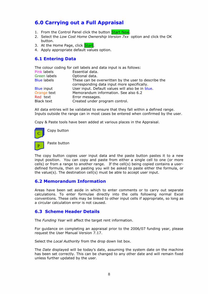
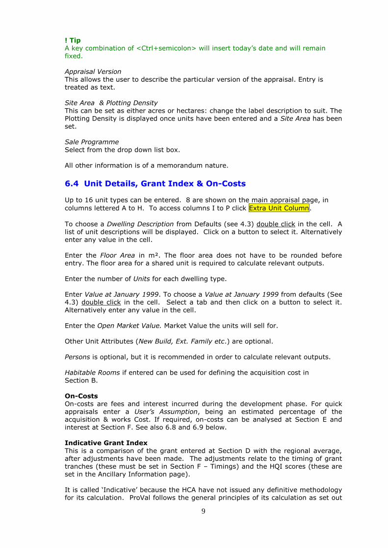
corresponding data input more specifically. Blue input User input. Default values will also be in blue. Orange text Memorandum information. See also 6.2 Red text Error messages. Black text Created under program control. All data entries will be validated to ensure that they fall within a defined range. Inputs outside the range can in most cases be entered when confirmed by the user. Copy & Paste tools have been added at various places in the Appraisal. Copy button Paste button The copy button copies user input data and the paste button pastes it to a new input position. You can copy and paste from either a single cell to one (or more cells) or from a range to another range. If the cell(s) being copied contains a user-defined formula, then on pasting you will be asked to paste either the formula, or the value(s). The destination cell(s) must be able to accept user input.

6.2 Memorandum Information

Areas have been set aside in which to enter comments or to carry out separate calculations. To enter formulae directly into the cells following normal Excel conventions. These cells may be linked to other input cells if appropriate, so long as a circular calculation error is not caused.

6.3 Scheme Header Details The Funding Year will affect the target rent information. For guidance on completing an appraisal prior to the 2006/07 funding year, please request the User Manual Version 7.17. Select the Local Authority from the drop down list box. The Date displayed will be today’s date, assuming the system date on the machine has been set correctly. This can be changed to any other date and will remain fixed unless further updated by the user.

C

P

9

! Tip A key combination of <Ctrl+semicolon> will insert today’s date and will remain fixed. Appraisal Version This allows the user to describe the particular version of the appraisal. Entry is treated as text. Site Area & Plotting Density This can be set as either acres or hectares: change the label description to suit. The Plotting Density is displayed once units have been entered and a Site Area has been set. Sale Programme Select from the drop down list box. All other information is of a memorandum nature.

6.4 Unit Details, Grant Index & On-Costs Up to 16 unit types can be entered. 8 are shown on the main appraisal page, in

columns lettered A to H. To access columns I to P click Extra Unit Column.

To choose a Dwelling Description from Defaults (see 4.3) double click in the cell. A list of unit descriptions will be displayed. Click on a button to select it. Alternatively enter any value in the cell. Enter the Floor Area in m². The floor area does not have to be rounded before entry. The floor area for a shared unit is required to calculate relevant outputs. Enter the number of Units for each dwelling type. Enter Value at January 1999. To choose a Value at January 1999 from defaults (See 4.3) double click in the cell. Select a tab and then click on a button to select it. Alternatively enter any value in the cell. Enter the Open Market Value. Market Value the units will sell for. Other Unit Attributes (New Build, Ext. Family etc.) are optional. Persons is optional, but it is recommended in order to calculate relevant outputs. Habitable Rooms if entered can be used for defining the acquisition cost in Section B. On-Costs On-costs are fees and interest incurred during the development phase. For quick appraisals enter a User’s Assumption, being an estimated percentage of the acquisition & works Cost. If required, on-costs can be analysed at Section E and interest at Section F. See also 6.8 and 6.9 below. Indicative Grant Index This is a comparison of the grant entered at Section D with the regional average, after adjustments have been made. The adjustments relate to the timing of grant tranches (these must be set in Section F – Timings) and the HQI scores (these are set in the Ancillary Information page). It is called ‘Indicative’ because the HCA have not issued any definitive methodology for its calculation. ProVal follows the general principles of its calculation as set out

10

by the HCA in their published documents. Further detailed information on the Grant Index calculation methodology is available from SDS on request.

6.5 Qualifying Scheme Cost Section B - Qualifying Scheme Cost - identifies all the capital costs of the scheme which qualify for grant. Confirm the floor area for the scheme at the start of the section. Make adjustments for circulation space etc. to the habitable floor area (entered in section A) by percentage and/or an actual figure. Floor area is an input option when entering acquisition and works costs, and when defining fees. Acquisition Replace the blue Text input with a suitable description, e.g. Asking Price, Agreed Value, My Guess. Select an Input Type from the drop down list box e.g. per unit, per person, lump sum etc. In the next column enter an Input value. Choose the VAT rate, if applicable, in the VAT % column. The Acquisition Total, averages per unit and per person are shown and, if entered, an averages per habitable room and per site area. Works Works costs entered in a similar way to Acquisition, by selecting an appropriate Input Type from the drop down list box (e.g. per unit, per person, lump sum etc.) followed by an Input value. VAT for any input can be added as appropriate. Choose the VAT rate in the VAT% column. The Works Total will be shown, together with averages per unit, per person and a total average per square metre (gross, gfa and habitable hfa). Account Codes Account Codes are used in conjunction with Export Data procedures. Sums can be transferred to other applications with an associated Account Code. Discount From On-Costs For 2006/07 funding years ignore this input. For earlier funding years, please refer to User Manual Version 7.17

6.6 Scheme Cost Index This only applies to schemes prior to 2006/07. For earlier funding years, please refer to User Manual Version 7.17

6.7 Grant At Section D enter a total Specified Gross SHG. This should include the value of RCGF and also the value of any free public land. Enter any other Public Subsidy (such as the value of free public land). When appraising schemes which have free public land, enter the full market value at Section B and show the value of the discount in the Grant section as Public Subsidy. The resulting Total SHG Claimed and grant rate will be displayed. Enter grant from other sources (compatible with SHG) together with a description of what the grant is, in Other Grant. It is recommended that LA capital grant is shown at this position rather than as SHG.

11

Sources of Grant can be set out as memorandum information. This information does not affect the viability results or the interest calculation in the development cashflow.

6.8 Analysis of On-Costs (Excl. interest) See Section E. Analysis of on-costs is optional. To analyse the on-costs set the Analyse On-Costs, y/n? to y. All descriptions and values can be set as defaults and amended on the appraisal. On-costs can be entered by two input alternatives:

1. In the column headed Input Type for Sums select from the drop down list box and enter an appropriate sum in the next column.

2. In the column headed Input Type for %. select from the drop down list box and enter an appropriate percentage in the next column.

Both options can be used together. The total displayed includes VAT where this option has been selected. See also Detailed On-Cost Timings [6.9.1]. Account Codes can be associated with each on-cost description and are used when exporting the data to other applications. To complete the analysis of on-costs calculate an estimate of the interest cost in Section F. See 6.9.

6.9 Scheme Timing Complete Section F to estimate the interest cost during the development period. This section is optional when not analyzing the on-costs, but the grant tranche timings are essential for the calculation of the Grant Index shown in Section A. Event timings in Section F create a Default Interest Cost. The user can subsequently amend monthly sums in the Scheme Cashflow and choose the interest arising. Detailed timings of fees can also be estimated, see 6.9.1. Begin by entering a Cashflow Start date using the format mmm-yyyy (e.g. Feb-2002). This date defines Month No.1. It is not an event but should not be set later than the earliest event in the cashflow. All subsequent cashflow timings must be entered as positive month numbers, relative to the Cashflow Start date. Set interest rates for negative and positive balances following the Cashflow Start. SHG Tranches Double click in the input cell and enter a percentage of the Total. Note that when the Total changes, the payment/sum will automatically change. If the Net Grant Tranche displayed is not correct an Alternative Net Tranche Sum can be entered in the adjoining column. Amend all tranches as necessary to ensure the total SHG remains the same. In the last column of this table enter the Receipt Timing by Month No. i.e. when each tranche will be received. The calendar date will be shown automatically. For example, if the Cashflow Start has been set to Jun-2006 then Month No.3 would be Aug-2006.

12

Other Grant A summary of any other grant entered is displayed on the right. Other Grant can be spread either by an S-curve (sine function) or by straight-line. Select preference from the drop down list box at Cost Spread Method. Complete timing information in the columns Receipt Start Month No. and Receipt End Month No. If the tranche is all received in one month, enter the same month no. in both columns. Acquisition Costs The acquisition total is shown on the right. This total can be split into 3 separate payments. For example, if monies are to be paid on exchange then this may be defined as the first payment and the balance paid on legal completion can represent the second or final payment. Double click in the input cell and choose either to create a sum based on a percentage of the Total, or to enter a formula linking the input to the Total. Note that when using a formula in this way, if the Total changes, the payment/sum will automatically change. Enter the Payment Timings by Month No. i.e. when each payment is due to be made in the last column of this table. If the acquisition value is being received as public subsidy, e.g. free land, then enter the actual land cost (enter zero if free) in the centre of this section. See also 6.7. Works Costs The works total will be shown on the right. Works can be entered into the cashflow as 3 separate sums, and spread, either by an S-curve (sine function) or by a straight line. Choose preference at Cost Spread Method. If there are high costs at the outset of the scheme then this amount may be treated as the First Sum and spread across the early months of the scheme with the balance being spread over another period(s). Double click in the input cell and choose either to create a sum based on a percentage of the Total, or to enter a formula linking the input to the Total. Note that when using a formula in this way, if the Total changes, the payment/sum will automatically change. For each sum entered under works costs enter an Expenditure Start Month No. and Expenditure End Month No. On-Costs Enter On-Costs in the same way as Works Costs, described above. Sales Programme Enter the Month No. for First Sale Month (i.e. when the first legal completion occurs) and similarly for Last Sale Month. Sales receipts are not entered as individual units; the income is spread evenly from first to last month number. Timings entered in Section F create a Default Interest Cost. To display the resulting cashflow on the Scheme Cashflow page:

1. Click Scheme Cashflow then click Update Cashflow Using Default Scheme

Timings/Sums.

2. This action will overwrite all existing sums unless "x" is entered at the top of the cost analysis column. A warning to this effect will be given.

3. Once displayed, the values can be amended by deleting or overwriting any value in blue.

13

4. Arithmetical errors will be shown by as a sum outstanding at the top of the column and by an error message.

5. To select the interest cost created by user specified sums, return to the Scheme Timings section and at the end of Section F, enter “y” at Substitute User-defined Sums - y/n?.

6. The Default Interest Cost can be selected at any time whether or not the Scheme Cashflow page reflects Scheme Timings, but any conflict between the Scheme Cashflow and the interest option selected will be highlighted.

Fees can be cashflowed separately by cost heading on the Detailed On-Cost Timings page and the resulting cashflow transferred to the Scheme Cashflow page [6.9.1]. A scheme can be cashflowed over a period of 48 months. For interest on land over a longer period, separately calculate the interest and add it as a capital cost in the Acquisition cost at Section B. The interest calculation in the month is calculated on the average cumulative cashflow balance at the beginning and end of the month.

To view the development cashflow as a chart click Cashflow Charts.

6.9.1 Detailed On-Cost Timings Create a detailed cashflow analysis of each individual on-cost as follows:

1. Click Detailed On-Cost Timings.

2. Each On-cost Description is displayed with its gross total (as defined in the Analysis of On-Costs - Section E).

3. To ensure a calendar date is assigned to each month number, enter a Cashflow Start in Scheme Timings (Section F).

4. The Balance to Enter total will reduce as sums are entered in the cashflow in columns headed 1 to 48. These can be manually entered.

5. Alternatively, each On-cost total can be automatically entered by clicking

the green button Automatically Spread On-Costs. Select an On-cost

description and define the spreading of costs in the dialog box displayed (3 separate spreading periods can be defined). Repeat the process for each On-cost Description.

6. On completion the detailed On-cost cashflow can be transferred to the

Scheme Cashflow by clicking Transfer Sums to Scheme Cashflow. Any

arithmetical errors will be flagged before transfer. On this page it is also possible to show the Paid to Date and Outstanding to Pay position for any specified date.

6.10 Comparison of On-Costs Section G compares the actual on-costs (fees and interest as analysed in Sections E & F) with the calculation arising from the percentage setting made in Section A. If a deficit arises, i.e. Total On-costs exceed Assumed On-costs this is displayed as a deficit and the deficit is added into the Total Scheme Cost in Section H. If the comparison results in a surplus, the surplus ignored in the Total Scheme Costs. In the case of a surplus the user is free to decide how the surplus should be used. To take the saving enter the surplus as a minus sum in Section H.

14

6.11 Summary of Total Scheme Costs Section H summarises the Total Qualifying Cost (as determined in Section B), together with any on-cost deficit identified when on-costs are analysed. Enter Non-Qualifying Costs together with any appropriate description. These costs do not attract grant. There are 2 entries for non-qualifying costs, but the user may also wish to use the facility at this position to make other adjustments to the total scheme costs. This section shows the comparison of Total Scheme Cost and its relationship with the Open Market Value of the units. A TSC/OMV Target % can be set to show the Affordable Total Scheme Cost. The Scheme Funding analysis displays the information entered in Section D on sources of SHG together with any loan adjustments from Section I.

6.12 Private Finance Section I defines the residual Net Loan which the scheme requires. The starting point is the Total Scheme Cost determined in Section H from which SHG and any other grant, together with sales receipts from the initial sales, are deducted. To recognise advance rent income, set the number of months ahead of practical completion that rent will be received. The amount of rent recognised is based on the Net Rent arising in Year 1 of the Long Term Cashflow, pro rata the number of months selected, then divided by 2. The loan can be further adjusted either by a user-defined Adjustment and/or by entering a RSL Capital Contribution. Neither entry will attract any funding costs. Entries made by an Adjustment or by a RSL Capital Contribution will be shown in the Analysis of RSL Funding in Section H. Loan Repayment Methods There are two methods of repaying the Net Loan.

Annuity The Annuity method repays both interest and capital over a specified term (up to 45 years) by a series of equal sums per annum (calculated monthly). This is similar to a conventional repayment mortgage. In the Long Term Cashflow the loan will always show as being fully repaid at the end of the Term, but a deficit may arise in the year if rent income is lower than the annuity. If surpluses arise later in the cashflow period any earlier deficits will get repaid. These deficits/surpluses are shown on the Cashflow line of the Long Term Cashflow and the Cumulative Balance is also shown.

Interest Only Method Interest, calculated on a monthly basis, is paid off year by year using all of the available Net Rent. If the net rent is greater than the interest, the outstanding loan is reduced. Conversely, if the net rent is less than the interest the outstanding loan will increase. This is akin to an overdraft. The Cashflow will only be shown in the Long Term Cashflow when the Loan is paid off.

15

Note that the loan may increase before rents are sufficient to exceed the interest charge and reduce the outstanding loan balance. In extreme cases the loan could increase infinitely.

Enter y to set the preferred Loan Repayment to the Annuity method or n for the Interest Only method. Interest Rates If appropriate, apportion the Net Loan into two loan sources by percentage, i.e. Loan A and Loan B. Set separate interest rates for each loan amount. Set Loan A:% Apportionment to 100% for a single loan source. Set interest rates for up to 3 periods. For the Annuity loan repayment method the rates must be set up to the term of the loan. For the Interest Only method rates must be set to Year 45 (the length of the Long Term Cashflow). Value:Loan Ratio At Section I OMV as % of Loan and Unsold Equity as % of Loan is displayed. Set an Unsold Equity:Loan, Target % to show the affordable loan. NPV of (Net Income + Net S/c Receipts) is shown separately, together with percentage to loan.

6.13 Inflation & Rent Allowances At Section J set the Base Inflation Rate e.g. RPI. Separate margins (positive or negative) are added to this rate for the rent income and rent allowances. Rents can be set over two periods. Management, Other Costs and Open Market Values are set over one period. All inflation parameters must be set to year 45. Allowances should be set at the rate equivalent to the first year that the scheme will be in management. Rent Allowances Set the allowances for the following: Management Set a sum per unit per annum. Other Costs This description can be changed by the user and a sum per unit per annum entered if appropriate. Voids & Bad Debts A percentage loss on gross rents.

6.14 Cost Rent at Year 1 At Section K enter the Number of Weekly Rent Periods to be collected in the year e.g. 52.18 (recommended) 48, etc. The Cost Rent at Year 1 to meet all Year 1 private finance repayments and other rent allowances is shown. Year 1 is the first full year that the scheme is in management.

16

When entering Advance Rent Income in Section I – Private Finance – the calculation of the Cost Rent ignores this income. The cost rent for each unit type is apportioned pro-rata to floor area. The cost rent for a unit which is shared is also treated in the same way. Warning! When the 'Interest Only' loan repayment method is used the calculation of Loan Interest in Year 1 is based on the full Net Loan. However, in the Long Term Cashflow an average interest is calculated after receiving rents. The Loan Interest in Section K will therefore not be the same as that shown in the Long Term Cashflow. Setting a rent equivalent to the Cost Rent may not repay the principal over the Long Term Cashflow unless there are sufficient revenue surpluses arising in later years.

6.15 Set Rents for Long Term Cashflow In Section L set the rent for each dwelling type. Rent should be set at a level appropriate to the time the units go into management. This rent determines the rent received in Year 1 of the Long Term Cashflow, i.e. the first full year that the scheme is in management. Rents are then inflated from Year 2 onwards. Remember that rent allowances set in Section J should also be as at Year 1 of the Long Term Cashflow. To show a rent based on the percentage yield of the unsold equity, enter Preferred Yield % on Unsold Equity at the start of this section. Enter Set Rent per Week into the dwelling column. On the next line enter any Other Charges p.w. to be collected. If the scheme does not require the payment of rent, enter zero. Check that any Other Charges collected are also matched by corresponding expenditure in Section J, as appropriate. E.g. Service charges collected will typically be equal to the cost of providing the service. If this is the case, the entries will not impact on the viability of the appraisal, but will have an effect on the affordability assessment in Section M. Affordable Loan The Affordable Loan is based on the rents set in this Section. The Net Rent received is capitalised at the Year 1 interest rate to show an Affordable Loan. The Affordable Loan is equivalent to what the RSL could afford to borrow on the Set Rents, assuming that the net rent in Year 1 fully met the loan cost in Year 1. For the 'Interest Only' loan repayment method, the loan cost is the interest cost in Year 1. For the 'Annuity' loan repayment method, the loan cost is the annuity in Year 1. A comparison between the Actual Loan with the Affordable Loan is reported as a Difference. If the Difference is negative it is the additional money (by way of subsidy or a reduction in the Loan) necessary for the Set Rents to breakeven at Year 1. If the Difference is positive, it indicates the amount of additional borrowing that the scheme could support. This Difference is also the Capitalised Year 1 Revenue Deficit/Surplus as shown in the Long Term Cashflow and is one way of assessing the implied capital subsidy required from the organisation.

17

6.16 Cost to Purchaser & Affordability Ratios Section M provides information on the level of mortgage required and based on the target income of the purchaser an indication of affordability. Schemes which appear acceptable to the RSL may still be unviable, because the purchaser costs are excessive and therefore, unaffordable. Such a position would undermine selling the units. Enter the Purchaser’s Mortgage Interest Rate and the mortgage Repayment Term. Enter a Target Total Cost/Earnings %. This target is the desired maximum ratio of the purchaser’s mortgage, rent and other costs to their gross earnings. A deposit can be paid by the purchaser, entered either as a percentage of the Open Market Value, or as a percentage of the equity share acquired. The effect is to reduce the mortgage and thereby improve affordability. Mortgage & Earnings Affordability Report This shows the minimum earnings required to qualify for the mortgage and the ratio of Total Costs to Minimum Earnings. If the ratio is greater than the target value, it is displayed bold. Enter a Mortgage Earnings Multiplier. This will determine the Minimum Earnings Required to qualify for the mortgage. E.g. If the purchaser requires equity of £50,000 then a mortgage multiplier of 3.5 would require minimum earnings of £50,000/3.5, i.e. £14,286 p.a. plus the annual cost of rent/other charges. Next, enter the gross Household Earnings p.a. expected to be earned. The maximum mortgage position is reported and the Total Cost/Household Earnings % displayed. Affordable Equity Share % Based on Household Earnings This report shows the affordable equity share based on the Household Earnings p.a. firstly, using the mortgage multiplier; secondly on the Target Cost/Earnings % The results are mutually exclusive. The inputs for Mortgage Earnings Multiplier and Household Earnings p.a. determine the maximum mortgage available to acquire an equity share. This share % is shown on the first line of the report, but the ratio of the total costs to the earnings may exceed the Target Cost/Earnings % as shown on the second line. Please note that the Affordable Equity Share % does not make any adjustment to the rent which may arise when increasing or reducing the equity share. LCHO Comparison with Outright Sale & Target Rent Buying the property outright by way of 100% mortgage determines the Outright Sale Cost p.w. (to which Other charges are added). The saving of the LCHO proposal is reported. If there is no saving then the result will be negative and shown bold. Also shown is the relationship between the cost of LCHO and the cost of outright sale. E.g. the total cost of a LCHO proposal to acquire 50% of the equity may be equivalent to 70% of the cost of outright sale. The higher the percentage the less attractive the proposal becomes (this ignores the question of earnings and mortgage status). A value greater than 100% would indicate that outright purchase is cheaper than LCHO and the result will show bold.

18

The Limited Target Rent is shown for comparison purposes only. Limited target rent is the lower of target rent and rent cap. The Extra Cost for LCHO p.w. is shown together with the Rent as % of LCHO. Averages for all of the above are displayed in the rightmost column.

6.17 Long Term Cashflow Section N shows the Long Term Cashflow (LTC) over 45 years. The cashflow is not intended to replicate the complex treasury arrangements which most organisations have. It is intended to show that the scheme, in isolation, can repay its loan and provide a viable return. 6.17.1 Cashflow Calculations 'Interest Only' Repayment Method This method treats the loan like an overdraft. The loan is repaid as soon as possible using the net rent plus any net staircasing receipts. The Average Interest assumes monthly rent and monthly loan repayments, but staircasing receipts are deemed to arise at the very end of the cashflow period. Total loan repayments are equal to the Loan Repayments arising from the Net Rent Received plus Staircasing Loan Repayments. When total loan repayments are greater than the loan interest, the Closing Loan reduces. Conversely, when they are less than the loan interest, the Closing Loan will increase. The Net Rent + Receipts - Less Interest (shown as memorandum text) is the difference between the Average Interest in the year and all net income. The Cashflow is the difference between all net income and all loan repayments and will therefore be zero until the loan has been repaid, at which point a positive Cashflow will arise. The Cumulative Balance adds together all Cashflows to the period up to Year 45.

'Annuity' Loan Repayment Method This method is similar to a conventional repayment mortgage. The loan is repaid by equal annual amounts (annuities) over the term specified in Section I. The Average Interest assumes monthly annuity repayments. Total loan repayments are equal to the annuity Loan Repayments plus Staircasing Loan Repayments. Total loan repayments may be higher or lower than the income available. The loan will always be paid off at the end of the term unless staircasing receipts allow the loan to be repaid sooner. The value of the annuity will change when interest rates change, as specified in Section I. The loan will always start reducing after Year 1 because the annuity includes interest plus loan principle. The Net Rent + Receipts - Less Interest (shown as memorandum text) is the difference between the Average Interest in the year and all net income. The Cashflow is the difference between all income and all loan repayments. The annuity remains constant year on year (assuming no change in the interest rate) but the rent increases by inflation, so revenue deficits which arise in the early years of the LTC may be met by surpluses in later years.

19

The Cumulative Balance adds together all Cashflows to the period up to Year 45. If at the end of the loan repayment period the Cumulative Balance is positive this represents the cash surplus arising at that point in time, but if it is negative, this is the total cash the organisation has given to the scheme; in either case, having first repaid the loan. 6.17.2 Cashflow Report Peak Loan Occurrence - shows the maximum loan amount and the year in which it occurs. For the 'Annuity' loan repayment method the peak loan will always be in Year 1, but for the 'Interest Only' loan repayment method the peak loan can be at any year and may increase indefinitely if the rents are set too low. If the result is n/a then the loan cannot be repaid within 45 years. Revenue First Exceeds Costs - for 'Annuity' loan repayment method, this will be the first year that total net income is greater than the total loan repayments. For the 'Interest Only' loan repayment method this will be the year that the total net income exceeds the Interest in the year. Loan Repaid By - for the 'Annuity' loan repayment method, this will always be the same as the term of the loan as set in Section I, unless staircasing receipts allow the loan to be repaid sooner. For the 'Interest Only' loan repayment method this will be the year in which the Closing Loan is zero. If the repayment period exceeds Year 45, then n/a will be displayed. See also Peak Loan Occurrence notes above. Peak Cumulative Debt - this will only be shown for the Annuity loan repayment method. The year and the amount will be shown. A debt arises when the Cashflow is negative (i.e. loan repayments exceed net income). The Cumulative Balance line will display the Peak Cumulative Debt. Ordinarily this will be the year before Revenue First Exceeds Costs – see above. First Cumulative Breakeven - this will only be shown for the Annuity loan repayment method and will be the first year in which the Cumulative Balance is positive. If there is more than one positive Cumulative Breakeven over the term of the cashflow, the last Cumulative Breakeven will also be reported. Last Cumulative Breakeven - this will only be shown for the Annuity loan repayment method and will be the last year in which the Cumulative Balance is positive. This will only be reported when there is more than one positive Cumulative Breakeven over the period of the cashflow. Maximum Annual Deficit – When the loan repayment method is Annuity, this will be the worst negative Cashflow in any one year. For the Interest Only method, it will be the worst shortfall between total net income and interest. Capitalised Year 1 Revenue Deficit/Surplus - this repeats the information described above in Section 6.15 –Affordable Loan. It is the difference between the Affordable Loan and the Actual Loan. If the reported amount were to be entered as an adjustment to the loan the cashflow will equal zero (Annuity loan repayment method) or the interest would equal total net income (Interest Only method). Cumulative Surplus/Deficit - the value of the Cumulative Balance at the year specified as Summarise Cashflow Results to Year. When the loan repayment method is Interest Only, this will be zero if the loan has not been repaid at the specified Cashflow Results to Year. Net Present Value (NPV)

1. Select an appropriate NPV Calculation Option from the drop-down list box (further explained below).

20

2. To include a residual Capital Value in the NPV enter values as prompted in this section, i.e.

a) Set the Capital Value of Scheme - Year 1, specify a Capital Growth Rate to inflate the year 1 value to the point in the future (as specified by Summarise Cashflow Results to Year). This value is discounted back to Year 1 and added to the NPV. The Discounted Capital Value is not shown in the LTC.

b) To include the Discounted Capital Value in the NPV calculation ensure NPV Calculation Option includes the Cap. Value option.

3. Enter a NPV Discount Rate. 4. Enter a period for the NPV calculation, Summarise Cashflow Results to Year.

There are 3 NPV Calculation Options. 1. Net Rent – Loan ( NPV net rent, minus the loan) 2. Net Rent + Cap. Value – Loan (NPV net rent, plus residual capital value and the

net staircasing receipts, minus the loan 3. Cashflow (NPV of the Cashflow line on the Cashflow) Net Rent – Loan The result is the net present value of the Net Rent Received (discounted over the period set at Summarise Cashflow Results to Year) from which the Opening Loan is deducted. The Opening Loan represents the initial capital costs to the organisation (i.e. Total Scheme Costs less grant). A positive result is normally required. Net Rent + Cap. Value – Loan is the same as above, except with this option a residual asset value can be defined. This is a value determined by the user as an estimate of what the capital value of the scheme will be at the point at Summarise Cashflow Results to Year discounted back to Year 1. It is not often used because the final result changes significantly depending on the estimate of residual value and hence it is not a very consistent measure. This option also adds in the NPV of the net staircasing receipts. This value is shown separately for information. Cashflow is the line shown on the Long Term Cashflow and represents the difference between the Net Rent Received and the Loan Repayments. When the loan repayment method is by Annuity and the loan interest rate and term are the same as the discount rate and NPV period, the result will be the same as Net Rent – Loan. When the loan repayment is Interest Only the result will represent the NPV of the net rent received after the loan has been repaid. Internal Rate Of Return - the IRR is related to the Net Present Value. It is the NPV Discount Rate which achieves a Net Present Value of zero. The Internal Rate of Return result displays the result according to the NPV Calculation Option chosen by the user. There are occasions when it is not mathematically possible to calculate IRR. Similarly the value may be greater than or less than 50%. In these instances the report will display either <-50% or >50% as appropriate. This should be interpreted as “No valid value found”. For NPV purpose the rent is discounted monthly. Yield Gross Yield is calculated as follows:

NPV of Gross Rent ex. Voids, divided by the Opening Loan, expressed p.a. (as defined by the prompt Summarise Cashflow Results to Year).

Net Yield is calculated as follows: NPV of Gross Rent ex. Voids less all allowances and Interest, divided by the Opening Loan, expressed p.a. (as defined by the prompt Summarise Cashflow Results to Year).

21

Interest - the Interest Total will be shown together with the year and value of the minimum interest cover. The interest cover is the Net Rent Received divided by the Interest arising in the year, as a percentage. Set a Target Interest Cover Percentage and the first year in which it will be met will be reported.

To see a graph of the LTC, click Charts at the top of the page. Two charts are

displayed below the Cumulative Development Cashflow, viz. 1. Annual Revenue Deficit/Surplus and the Cumulative Balance. 2. Closing Loan Profile.

6.18 Staircasing Staircasing can be entered in Section N by spreading the total unsold equity

percentage. There is a tool to enable automatic spreading. Click Set/Clear

Stairc’sg Profile and follow on-screen instructions.

Use the option Inflate Grant/Equity Loan by OMV inflation when staircasing, y/n? to inflate the grant/equity loan by the value of the OMV inflation factor when staircasing. An Equity Loan is similar to Grant except the repayment of it is indexed to the sales receipts and so the repayments can therefore eventually exceed the amount of the initial sum provided. Sequence of Transactions When a Unit Staircases 1. The Shared Unsold Equity is inflated (from year 2) up to the year in which

staircasing occurs. 2. The Year End Receipt is based on the Staircasing % to be Sold entered by the

user. 3. From the receipt the deemed loan debt repayment (pro rata to the Staircasing

% to be Sold) is made and is shown as the S'csg Loan Repayments. If there is insufficient receipt to meet the deemed loan debt then all of the receipt is used to reduce the loan and no payment to the Grant Recycling Fund is made.

4. From the remaining receipt the grant is set aside to the Grant Recycling Fund. The grant is pro rata to the Staircasing % to be Sold.

5. If the remaining receipt is insufficient to make a full payment to the Grant Recycling Fund, the shortfall will be shown as Grant Deferred and is carried forward to the next staircasing event.

6. Any remaining surplus after step 5 is used to make further Staircasing Loan Repayments. If the Loan Repayments from Staircasing allow the loan to be repaid in full, any balance is shown in the Cashflow.

7. After staircasing, the unsold equity will reduce and the rent received in the following years will also reduce pro rata. Other Charges are not affected.

7.0 Sensitivity Analysis The Sensitivity Analysis shows the effect of changing 13 key variables, Scenarios, on the Long Term Cashflow position. The Analysis also calculates the Scenarios J & K separately report the additional subsidy, rent change or equity share to meet a particular loan repayment period (Interest Only loan repayment method) or Cumulative Cashflow period (Annuity method). The results will report the combined effect of all scenarios specified, except Scenarios J & K. For these scenarios all current appraisal parameters/input remain unchanged, including grant.

22

When On-Costs are analysed the interest calculation may be set to user-specified. In this situation when testing sensitivity of capital costs (i.e. Acquisition, Works or the Grant) it is not possible to automatically recalculate the interest, therefore the sensitivity analysis ignores the impact of interest changes. When these conditions apply a note to this effect is displayed in the Results section. To show the Sensitivity results for the scenarios specified by the user, click

Show Sensitivity Results.

When printing the Sensitivity Report the user will be prompted to Update the Sensitivity Analysis. This is to ensure that the printed results correctly report the sensitivity results based on the current appraisal position. Refusing to update the Analysis will cause the report to be printed without the Results section completed.

8.0 Benchmarks The Benchmarks page allows the user to compare benchmark values with current Appraisal values. Benchmark values are defined at 3 levels and must be set in the Defaults file [see 4.0]. The levels are: Green: A benchmark value which you want to meet. If the Appraisal passes this

test a green traffic light is displayed. Amber: Logically any value between Green and Red. Red: A benchmark value which you do not want to exceed. If the Appraisal

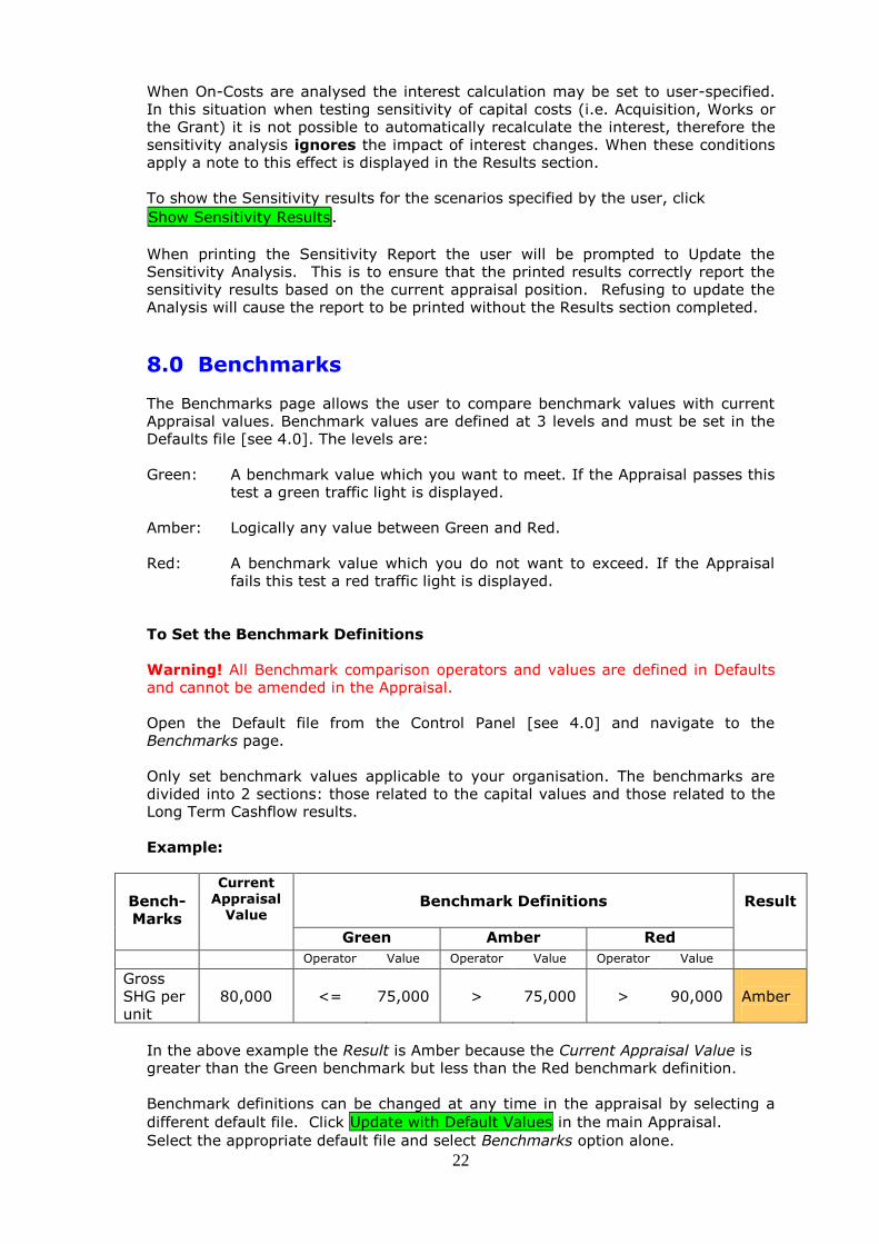
fails this test a red traffic light is displayed. To Set the Benchmark Definitions Warning! All Benchmark comparison operators and values are defined in Defaults and cannot be amended in the Appraisal. Open the Default file from the Control Panel [see 4.0] and navigate to the Benchmarks page. Only set benchmark values applicable to your organisation. The benchmarks are divided into 2 sections: those related to the capital values and those related to the Long Term Cashflow results. Example:

Bench- Marks

Current Appraisal

Value

Benchmark Definitions

Result

Green Amber Red

Operator Value Operator Value Operator Value

Gross SHG per unit

80,000

<=

75,000

>

75,000

>

90,000

Amber

In the above example the Result is Amber because the Current Appraisal Value is greater than the Green benchmark but less than the Red benchmark definition. Benchmark definitions can be changed at any time in the appraisal by selecting a

different default file. Click Update with Default Values in the main Appraisal.

Select the appropriate default file and select Benchmarks option alone.

23

At the bottom of the page of this report the user can define and set appraisal descriptions/values not already listed in the first two sections as follows. To define other benchmarks

1. Unhide Sheet Tabs by clicking Reveal or Hide Tabs at the top of the page. Click

OK when the warning message appears. 2. Enter a description for the benchmark. If the benchmark value is a value per

unit or per person, use the 6 lines at the top of this section. If the benchmark value is a percentage, enter its description in the last 8 lines of this section.

3. Enter the Current Appraisal Value to be benchmarked in the second column by using an Excel formula e.g.

a. Enter an = sign in the cell b. Choose the Appraisal sheet tab at the bottom of the screen to c. Highlight the Appraisal page d. Click in the cell which holds the value you want to benchmark e. Press Enter button on keyboard.

4. Hide the Sheet Tab by clicking Reveal or Hide Tabs at the top of the page.

5. Enter Green and Red Benchmark Definition Operators and Values.

9.0 Printing

All printing is done from a single print button Printing Options shown at the top of

the page. Any combination of pages and quantity can be printed. Pages can be printed in colour if preferred. Uncheck the Black & White option. The default printer will be shown on the Print Options dialog box, but other printers can be selected. To set the default printer:

1. Click Set Defaults on the Control Panel.

2. Choose the Personal Defaults option. 3. Click into the cell and choose a printer from the printer names listed.

4. Click Save & Return to Control Panel.

When printing the Sensitivity Report the user will be prompted to Update the Sensitivity Analysis. This is to ensure that the printed results correctly report the sensitivity results based on the current appraisal position. Refusing to update the Analysis will cause the report to be printed without the Results section completed. Printing Default Values It is not possible to print the Personal Defaults information. Printing System Defaults To print the default values’ files:

1. Click Set Defaults on the Control Pane.

2. Choose the default file to be printed.

3. When the file opens click View Defaults.

4. Navigate to the page to be printed.

5. Click Print this Page. The device will be the active printer. A printer

24

dialog box will not be displayed and one copy of the page will be printed. 6. Repeat Step 4 and 5 to print other pages.

10.0 Exporting Data Where the remote system requires A/c Codes, these can be set as defaults. To set these default values see [4.0]. To create an export data file: 1. Open appraisal from which the data is to be exported.

2. Click Home page.

3. Click Create Export Data File .

4. Select the type of file to be created. Those systems which are supported will be displayed.

5. Follow the on-screen instructions. 6. A file will be saved on completion and stored in the current appraisal folder. 7. Once an export file has been created, it is then ready to import into the remote

system. Follow the remote system's instructions for doing this. Subsequent Appraisal Changes After an export file has been created it will not be updated if the appraisal data is subsequently changed. To create a new export file of a changed appraisal file, repeat steps 1 to 7 above. A message will be displayed warning that an export file already exists which can then be overwritten. Once overwritten the previous export file will be lost. To avoid this happening save the updated appraisal file as a new version with a new file name. See [2.4] for help with this.

11.0 Help

For on-screen help, click Help.

For individual Help topics click the button Index, View Topic & Print.

From the list of topics displayed, select a topic and click the button View Topic. To

print the topic note click the button Print Topic.

If the page is not optimally displayed for your screen, click

To return to the Appraisal click the button Return to Appraisal

Some cells on the Appraisal have user help notes in a comment box. Comment boxes are identified by a small red triangle in the top right corner of the cell. To view the comment, place the mouse cursor over the red triangle. See also thewww.sdsproval.co.uk website for FAQS and other topical help notes.

Resize Page Widths

25

Appendix Creating Links & Entering User Defined Calculations The following instructions are for users with a basic understanding of Microsoft Excel. Entering User Defined Calculations

1. In an open ProVal Appraisal file, create a calculation in a Memorandum Area using normal Excel formulae. E.g. =SUM(source range)

2. The result must usually be a whole number and not equal to zero, otherwise in the next step the ProVal data validation procedure may either reject it, or ask you to accept it.

3. To enter the result into the appraisal, click into the destination cell (which must be capable of receiving user input) and type an = sign. Point to the cell in the Memorandum Area which holds the source value and <Enter>. To ensure a whole number is entered use the Excel ROUND function. E.g. In the destination cell type:

4. =ROUND(source cell address,0) 5. To break the link delete the data in the destination cell. 6. Alternatively, you can enter a formula directly into a destination cell. In this

case watch that you do not create a Circular calculation. If this happens you will see an error message in the Status Bar.

Warning! Values which are entered using a formula can cause problems, if the user forgets that the formula exists. Values on the appraisal may change unexpectedly, depending on whether the precedents are changed. Use formulae with caution. Creating Links to Other Excel Workbooks

1. Open a ProVal Appraisal file from the Control Panel and go to the part of the Appraisal which has the relevant data.

2. Start a new instance of Excel (Windows | Start | Programs). 3. Start a new workbook. 4. In a cell of the new workbook type an = sign 5. Return to the ProVal appraisal using the icon on the Status Bar. 6. Click into the source cell (a dotted line will appear around it) and press

<Enter> You can now edit the cell of the new file using normal Excel functions. When the new workbook is saved the links to the Appraisal will also be saved. On opening the new workbook the user will be prompted to update the link. Agreeing to update the link will amend the destination values with the current Appraisal values.