User Guide - Novoptel

User Guide

PM1000 Polarimeter

Novoptel GmbH

EIM-E

Warburger Str. 100

33098 Paderborn

Germany

www.novoptel.com

Revision history

Version Date Remarks Author

0.2.1 26.01.2015 Draft version B. Koch

0.2.2 27.02.2015 Register and operation description updated B. Koch

0.2.3 04.03.2015 Operation description updated B. Koch

0.2.4 11.03.2015 Description of measurement data files B. Koch

0.2.5 21.07.2015 Description of PDL measurement B. Koch

0.2.6 24.07.2015 Remove obsolete registers 96 to 102 B. Koch

0.2.7 05.04.2016 Includes all functions until firmware 1.0.2.1 B. Koch

0.2.8 20.06.2016 GUI v1.0.7.1, firmware 1.0.3.1: 100 MS/s Poincaré live

view, delay of BNC trigger input, optional 720p60 output

B. Koch

0.2.9 24.01.2018 GUI v1.0.9.5, firmware 1.0.4.5: Add description of laser

modulation / demodulation, high-sensitivity mode

B. Koch

0.3.0 20.08.2018 GUI v1.1.0.0, firmware 1.0.5.0: Simultaneous recording

and data transfer; variable pre- and post-trigger data

B. Koch

0.3.1 02.05.2019 Firmware 1.0.5.1: Power transient detection, LAN B. Koch

0.4.0 09.06.2020 GUI 2.0.0.0; firmware 1.0.6.0: Dynamic undersampling,

laser sweep

B. Koch

0.4.1 28.07.2020 Add USB 3.0 transfer protocol and SDRAM data transfer B. Koch

0.4.2 27.08.2020 Minor changes in Register description; retrigger during long

events (firmware 1.0.6.2)

B. Koch

0.4.3 12.05.2021 Add registers for trigger input 2 (from laser, fw 1.0.6.6); add

scrambler voltage calibr. for <4 SOPs; configuration files

B. Koch

0.4.4 12.07.2021 PM1000 clock drift compensation during SOP event

recording (fw 1.0.7.0). Register for reference SOP table

B. Koch

0.4.5 15.09.2021 Modification of reference SOP table registers (fw 1.0.7.2),

extend description of Wavelength sweep

B. Koch

Novoptel 3 of 54 PM1000_UG_0_4_5_k01.doc

Table of contents

Introduction ................................................................................................................. 5

Rear panel .................................................................................................................. 5

External monitor ......................................................................................................... 5

Fundamental PM1000 configuration ........................................................................... 6

Register description .................................................................................................... 7

Reference SOP table memory .................................................................................. 13

Reset dark current ................................................................................................ 15

Sphere: live / memory ........................................................................................... 15

Connecting the instrument to a PC via USB ............................................................. 16

Installing the USB driver ........................................................................................ 16

Connecting the instrument .................................................................................... 16

Operation of the instrument via graphical user interface .......................................... 17

Standalone GUI .................................................................................................... 17

Installing GUI ........................................................................................................ 17

Basic operation ..................................................................................................... 18

User Settings ........................................................................................................ 22

Memory configuration............................................................................................ 24

Triggering and gating ............................................................................................ 26

Internal trigger configuration ................................................................................. 27

User calibration set ............................................................................................... 30

Device Test ........................................................................................................... 31

Wavelength Sweep ............................................................................................... 35

Laser Modulation / Demodulation ......................................................................... 39

Input Power Histograms ........................................................................................ 41

SOP Speed Histograms ........................................................................................ 41

Using Matlab to analyze stored data ..................................................................... 43

Operation of the instrument using register access .................................................... 47

Access the USB driver .......................................................................................... 47

Support for Matlab ................................................................................................ 47

USB 2.0 Settings ................................................................................................... 47

USB 2.0 Transfer protocol ..................................................................................... 47

USB 3.0 Transfer protocol ..................................................................................... 49


TCP/IP (LAN) Communication .............................................................................. 51

SPI Communication .............................................................................................. 52

Serial interface (SPI) commands .......................................................................... 52

Serial interface (SPI) timing .................................................................................. 52

Operation of the instrument using other programs ................................................... 54

Firmware upgrade .................................................................................................... 54

Acronyms .................................................................................................................. 54


Introduction

The PM1000 polarimeter measures all 4 Stokes parameters at a sampling rate of 100 MHz.

Optionally, the samples are averaged to increase accuracy at low optical input power.

Furthermore, three normalization modes can be chosen. The calculated states of polarization

(SOPs) are displayed on a Poincaré sphere at a connected monitor. This allows the

polarimeter to be used without extra computer. The external monitor shows the realtime

Poincaré sphere display at up to 50 MHz (at 100 MHz, only every second sample is

displayed).

To explore the temporal evolution of the polarization, the user can switch the display to

oscilloscope view. In this mode, the Stokes parameters are recorded in the polarimeter’s

memory and then plotted over time. The memory size is 4.3 Gb, i.e. 67 M polarization states

can be recorded. The user can shift the oscilloscope plot and zoom into via the front control

buttons.

The recording process can be triggered either externally by a BNC input signal or internally

by defined SOP or input power events. Pre- and post-trigger data is stored. The memory can

be read out via the SPI or USB interface. To configure the polarimeter, a graphical user

interface (GUI) can be started on a PC that is connected to the polarimeter by USB. The GUI

can also load screenshots of the connected monitor to the PC and display the Poincaré

sphere.

Rear panel

Figure 1 shows the rear panel of the PM1000.

Fig. 1: PM1000 rear panel.

External monitor

A monitor can be connected to the HDMI output to display a polarimeter screen with 1280 x

720 pixels (“720p”, now default) at 60 Hz. A HDMI to DVI cable is included. It must be

ensured that the connected monitor supports the chosen display standard!

BNC

+5V IN

AIR IN

AIR OUT POWER SWITCH


Fundamental PM1000 configuration

Optical frequency

The optical frequency value can be adjusted to match that of the analyzed optical input signal.

Averaging time (ATE)

For accurate SOP measurement at lower optical input powers, internal averaging after the 100 MS/s AD conversion is recommended. The averaging time is denoted by the averaging time exponent (ATE). 2ATE samples are averaged and an effective conversion time of

2ATE10 ns is achieved. ATE ranges from 0 (100 MS/s) to 20 (95.4 S/s).

Normalization mode

The PM1000 provides three choices for the normalization of Stokes parameters/ vectors:

Standard normalization: Stokes vectors are normalized to unit length. Regardless of power and DOP, they appear at the surface of the Poincaré sphere.

Exact normalization: Stokes vectors are normalized only with respect to optical power. For DOP < 1 (or DOP = 0) they appear inside (or in the center of) the Poincaré sphere.

Non-normalized: Stokes vectors are normalized only with respect to a user-defined power value, 1 mW by default. This means that DOP and optical power determine the length of the displayed Stokes vector up to a maximum length of 1.

Memory exponent (ME)

The memory exponent (ME) defines the size of the internal memory block that is being

written into. The smallest block is achieved with ME=10 (210 = 1024 SOPs). The largest block

is achieved with ME=26 (226 = 67,108,864 SOPs).

The memory recording time is derived from ME, ATE and the sampling time 10 ns. At highest

speed (ATE=0), the memory is filled within 0.67 seconds, since 226∙20∙10 ns = 0.67 s.


Register description

Basic functions of the PM1000 are configured using the front control buttons. Advanced

functions can be controlled through the USB, LAN or SPI port by reading and writing to

internal registers, which are described in the following table. Note that the register addresses

have an offset of 512. This allows a Novoptel PM1000 polarimeter and an EPS1000

polarization scrambler/transformer to be connected to a shared single SPI port. All undefined

registers are reserved and should not be written into.

Register

address

Name Bit(s) Read/

Write

Function

512+0 ALM Internal alarm code. The alarm can be cleared by

writing “0” to this register. This is successful only if

the alarm condition is no longer present.

0 R/W Alarm condition present.

1 R/W Optical input over range.

2 R/W Optical input under range.

4 R/W Critical board temperature.

512+1 ATE 9..0 R/W Averaging time exponent (ATE), integer range 0 to

20.

512+2 PC1 15..0 R Photocurrent 1, 16 bit unsigned, averaged according

to ATE.


to ATE.


to ATE.


to ATE.

512+6 LPC2 15..0 R Latched copy of photocurrent 2, updated on any read

of PC1.


of PC1.


of PC1.

512+9 PCFP 15..0 R Floating point position of photocurrent 1 to 4,

updated on any read of PC1.

512+10 S0uWU 15..0 R Input power in µW, integer part.

512+11 S0uWL 15..0 R Input power in µW, fractional part. Updated at last

read of S0uWU.

512+12 S1uWU 15..0 R S1 of Stokes vector normalized to 1 µW, integer part.

Offset=215.

512+13 S1uWL 15..0 R S1 of Stokes vector normalized to 1 µW, fractional

part. Updated at last read of S1uWU.


Offset=215.




Offset=215



512+18 LS1uWU 15..0 R Latched copy of S1uWU, updated on any read of

S0uWU


512+19 LS1uWL 15..0 R Latched copy of S1uWL, updated on any read of

S0uWU


S0uWU


S0uWU


S0uWU


S0uWU

512+24 DOPSt 15..0 R Degree of polarization (DOP), 16 bit unsigned, 15

fractional bits

512+25 S1St 15..0 R S1 of Stokes vector “Standard Normalization”, 15

fractional bits. Offset=215.





512+28 LS1St 15..0 R Latched copy of S1St, updated on any read of

DOPSt


DOPSt


DOPSt

512+31 DOPEx 15..0 R Degree of polarization (DOP), 16 bit unsigned, 15

fractional bits

512+32 S1Ex 15..0 R S1 of Stokes vector “Exact Normalization”, 15






512+35 LS1Ex 15..0 R Latched copy of S1Ex, updated on any read of

DOPEx


DOPEx


DOPEx

512+38 EPow 15..0 R/W Reference power level in µW for non-normalized

Stokes vectors to reach a length of 1.

512+39 S1Nn 15..0 R S1 of Stokes vector “Non-normalized”, 15 fractional

bits. Offset=215.


bits. Offset=215.


bits. Offset=215.

512+42 LS2Nn 15..0 R Latched copy of S2Nn , updated on any read of

EPow


EPow


EPow

512+45 S3Sign 0 R/W If 1 (default), sign of S3 is chosen so that transversal

directions x and y form a right-handed coordinate


system with propagation coordinate z.

512+46 SlNrm 1..0 R/W Stokes parameters/vector normalization mode, see

section Fundamental PM1000 configuration.

“00”: Non-normalized

“01”: Standard normalization

“10”: Exact normalization

512+48

…

512+63

UCal 15..0 R/W User calibration matrix M with elements M00, M01,

M02, M03; M10, M11, M12, M13; M20, M21, M22,

M23; M30, M31, M32, M33. Non-normalized Stokes

vector = M (photocurrent vector).

512+64 UCalSL 3..0 R/W Floating point position of user calibration matrix.

512+65 SelUCal 0 R/W “1” switches to user defined calibration matrix.

1 W “1” writes user calibration matrix to flash RAM.

512+66 WLBand 9..8 R Number of available wavelength bands

1..0 R/W Index of current wavelength band

512+67 MinFreq 15..0 R Minimum extrapolated optical frequency in GHz/10,

16 bit unsigned.

512+68 MaxFreq 15..0 R Maximum extrapolated optical frequency in GHz/10,

16 bit unsigned.

512+69 CurFreq 15..0 R/W Current optical frequency in GHz/10, 16 bit unsigned.

512+70 MinCalFr 15..0

R

Minimum calibrated optical frequency in GHz/10, 16

bit unsigned.

512+71 MaxCalFr 15..0 R Maximum calibrated optical frequency in GHz/10, 16

bit unsigned.

512+72

0 W SDRAM write trigger. Any write of “1” to this register

bit will trigger a recording of the sampled SOPs in the

SDRAM. Recording period is defined by averaging

ATE (register 512+1). 2ME samples will be recorded,

defined by the memory exponent ME (register

512+73).

Writing of “0” into this bit will stop any recording in

progress. (3)

R SDRAM busy. ”1” if recording is in progress.

1 R “1” if post-trigger data recording is in progress.

2 R/W Continuous cyclic memory recording enabled (1) or

disabled(0)

3 R “1” if a full memory block was recorded since the last

trigger

W “1” enables automatic retrigger for next memory

block

4 R “1” if SDRAM is busy due to oscilloscope display

W “1” enables “endless” retrigger for next memory

block. Restarts in block 0 if end or memory is

reached, pauses if block number specified in register

(512+82) is reached. (1)

5 R “1” if SDRAM is busy due to Poincaré sphere display

8 R/W Enables dynamic undersampling(3)

10 R/W Enables retriggering during long events(4)

15 R “1” if endless block retrigger is paused (1)

512+73 4..0 R/W SDRAM memory exponent ME (max. 26)

512+74 3..0 R/W Negative exponent for 16 bit power vector recorded

to SDRAM. The recorded data represents power in


µW left-shifted bitwise by this value. The shifting

reduces quantization errors when recording at low

input powers.

512+75 0 R/W “0” selects Power+Stokes to be recorded, “1” selects

DOP+Stokes

1 R Power/DOP selection updated at last SDRAM trigger

512+76 15..0 R Current write address of SDRAM, bits 15..0

512+77 9..0 R Current write address of SDRAM, bits 25..16

512+78 15..0 R The number of recorded Blocks after last SDRAM

trigger

512+79 15..0 R/W Selects a memory block

512+81 9..0 R/W The stop address in the selected memory block, bits

25..16. Used in combination with register (512+96). (7)

512+82 15..0 R/W Maximum number of memory blocks in automatic

retrigger mode. Default is 512. In endless retrigger

mode, recording is paused when it reaches the block

defined by this register. (1)

512+83 15 R/W Defines power event trigger source:

“0”: Selects power deviation from reference

“1”: Selects power gradient (power increases or

decreases by more than given factor within given

time)(2)

14..0 R/W Factor (>1) for power gradient detection as 15 bit

unsigned including 10 post-comma bits (2)

512+84 15..0 R/W Input power trigger threshold in µW

512+85 15..0 R/W Input power reference in µW

512+86 0 R/W Define reference for internal trigger signal:

“0”: External Stokes vector

“1”: Internal delayed Stokes vector

6..1 R/W Number of clock cycles -1 for Stokes vector delay

10..7 R/W Exponent for clock division of Stokes vector delay

512+87 15..0 R/W Stokes parameter 1 of external Stokes vector

reference. 15 fractional bits. Offset=215.





512+90 15..0 R Current internal SOP trigger signal

512+91 15..0 R/W Trigger threshold for internal SOP trigger signal

512+92 0 R/W “1” enables SOP event triggering.

1 R/W “1” enables SOP event gating.

2 R/W SOP event triggering/gating: “0”: Active high/rising

edge. “1”: Active low/falling edge

3 R/W “1” enables external triggering through BNC.

4 R/W “1” enable external gating through BNC.

5 R/W External triggering/gating: “0”: Active high/rising


6 R/W “1” enables input power event triggering.

7 R/W “1” enables input power event gating.

8 R/W Input power triggering/gating: “0”: Active high/rising


12..11 R/W Trigger2 input (from laser) configuration:

“00”: Ignore trigger2. No timestamps


“10”: Record all SOP vectors according to registers

(512+96) and (512+81) after rising edge of trigger2.

Add a timestamp after every first SOP vector of a

cycle defined by register (512+103).

“01”: Record one SOP vector cycle defined by

register (512+103) upon each rising edge of trigger2.

Add a timestamp after every first SOP vector of a

cycle.

512+93 15..0 R Bits 47..32 of internal microseconds counter. Bits

31..0 are frozen when reading this register. (6)

512+94 15..0 R Bits 31..16 of internal microseconds counter. (6)

512+95 15..0 R Bits 15..0 of internal microseconds counter. (6)

512+96 15.0 R/W Memory (SDRAM) recording stop address:

If >0, the memory recording will stop at this address.

If 0, recording will stop at the address 2ME-1. Used in

combination with register (512+81).

512+103 10..0 R/W Number or SOPs to be recorded for one Mueller

matrix. Used in combination with register (512+92) (5)

512+104 15..0 W Code 39293 triggers SDRAM USB high speed

transfer. Code 39294 triggers SDRAM LAN high

speed transfer.

512+105 15..0 R/W Bits 15..0 of SDRAM high speed read address

512+106 9..0 R/W Bits 25..16 of SDRAM high speed read address

512+107 15..0 R/W Number of addresses to be transferred in SDRAM

high speed mode.

512+108 15..0 R/W Power threshold in µW under which SOP triggers are

blocked (1). Default value: 1 µW

512+110

…

512+125

15..0 R Factory calibration matrix M with elements M00,

M01, M02, M03; M10, M11, M12, M13; M20, M21,

M22, M23; M30, M31, M32, M33. Non-normalized

Stokes vector = M (photocurrent vector).

512+126 3..0 R Floating point position of factory calibration matrix.

512+127 15..0 R/W Delay for optional trigger input 2 (from laser) in

microseconds

512+128 15..0 R Firmware version as 4 digit BCD

512+129 15..0 R Device DNA word 3 (DNA bits 63...48) (same as

read via JTAG)


read via JTAG)


read via JTAG)

512+132 15..0 R Device DNA word 0 (DNA bits 15...0) (same as read

via JTAG)

512+133 15..0 R Module Serial Number

512+134 15..0 R Maximum input power in µW

512+144

…

512+159

15..0

R Module Type as 32 character string. Beginning at

512+144, each Register contains two bytes,

representing two ASCII-coded characters.

512+186 0 R/W Selects display type at connected monitor:

“0” selects Poincaré sphere live view

“1” selects Poincaré sphere memory view

512+187 0 R/W “1” enables automatic Poincaré sphere refresh

512+188 15..0 R/W Automatic Poincaré sphere refresh period in

milliseconds, 16 bit unsigned


512+189 15..0 W Any write transaction to this register clears the

Poincaré sphere on the connected monitor.

512+201 1..0 R/W Determines the pre-trigger data amount (1)

“00”: 50%, “01”: 25%, “10”:12.5%

512+202 15..0 R/W Stokes parameter threshold for dynamic

undersampling as integer in rad * 215

512+203 0 R/W “1” enables synchronization of averaging to edge of

sync signal at BNC input4)

512+204 4..0 R/W If >0: Maximum ATE during dynamic undersampling

512+207 0 R/W “0” freezes HDMI frame buffer

512+220 0 R/W 1 (default): Enable bit-shift of ADC values to reduce

quantization errors.

1 R/W 1 (default): Increase averaging at low input power to

reduce noise.

512+226 15..0 R/W BNC input debounce time * 10 ns. At 50 (default), the

status of the input is adopted after 500 ns without

toggling.

512+227 8..0 R/W BNC input delay time * 10 ns. At 10 (default), the

signal is delayed by 100 ns. Bits 8 and 7 exist only in

firmware 1.0.3.1 or newer

12..9 R/W Only in firmware 1.0.3.1 or newer:

Clock exponent for BNC input delay line.

15..13 R/W Only in firmware 1.0.3.1 or newer:

Number of BNC trigger events that are ignored after

every activation of a recording.

512+229 15..0 R Returns the power histogram count according to

histogram address and bit selector

512+230 9..0 R/W Histogram address

15..14 R/W Histogram bit selector

“00”: Bits 15..0 of histogram count are read

“01”: Bits 31..16 of histogram count are read

“1X”: Bits 47..32 of histogram count are read

512+231 15..0 R Returns the SOP speed histogram count according

to histogram address and bit selector

512+232 3..0 W Histogram control

Bit 0: “1” starts the SOP speed histogram count.

Bit 1: “1” stops the SOP speed histogram count.

Bit 2: “1” starts the power histogram count.

Bit 3: “1” stops the power histogram count.

512+234 3..0 R/W SOP speed histogram right shift bits. With a value he

given by this register, the maximum histogram bin

(address 1023) refers to 8 rad / 2he.

512+236 5..0 R/W Number of clock cycles for SOP speed interval

10..6 R/W Exponent for clock division of SOP speed interval

512+237 1..0 R/W Input power histogram selector

“00”: The current input power value is recorded

“01”: The power difference between current and

delayed value is recorded

6..3 R/W Power histogram right shift bits. With a value he

given by this register, the maximum histogram bin

(address 1023) refers to 8192 µW / 2he.

512+238 5..0 R/W Number of clock cycles for power interval

10..6 R/W Exponent for clock division of power interval

512+300 15..0 R/W Reference Timestamp Bits 63..48(3)





512+430 1..0 R/W Status of the optional optical switches. Bit 0 refers to

first switch, Bit 1 to second switch. Usually first

switch is REF/DUT and second switch inverts light

path through DUT.

512+445 1 W “1” will reset the table to the first entry(7)

0 W “1” will launch a trigger event (manual trigger) (7)

9..0 R Read current Ref. SOP table position(7)

512+446 5..0 W Ref. SOP table memory write trigger. (7)

Bit 0: Write table memory vector 00

Bit 1: Write table memory vector 01

…

Bit5: Write table memory vector 05

512+447

8

R/W

Enable (1) or disable (0) ref. SOP table(7)

1 R/W Enable (1) or disable (0) continuous table

execution(7)

0 R/W Table execution in row (1) or table (0) mode(7)

512+448 10..0 R/W Length of current table in table memory(7)

15..12 R/W Table trigger divider exponent x. Example for x=3:

Only every 8th (23=8) trigger event will be processed.

(7)

512+449 9..0 R/W Table memory input address(7)

512+450

…

512+454

15..0 R/W Table memory input vector 00 to 04. See section

“Reference SOP table memory”. (7)

512+460

…

512+464

15..0 R/W Table memory output vector 00 to 04. See section

“Reference SOP table memory”. (7)

(1) Only applicable since firmware 1.0.5.0







Reference SOP table memory

Since firmware 1.0.7.1, the reference SOP for the triggering and tracking function can be

taken from an internal table memory. The table memory is either triggered row by row by an

external signal at the BNC port of the polarimeter, or it runs in continuous mode with dwell

times specified in each table row.

Vector Meaning

00 Table dwell time in multiples of 40 ns, minus 1, Bits 15..0

01 Table dwell time in multiples of 40 ns, minus 1, Bits 31..16

02 Stokes parameter 1 as 16 bit signed integer with 15 fractional bits




For a dwell time of 200 ns, a value of 4 must be written into Vector 00, since

(4+1)*40ns=200ns. A Stokes parameter of -0.123 must be written as 61506 since 2^16-

round(0.123*2^15)= 61506.


Operation of the instrument via front control panel

The polarimeter firmware provides a cyclic menu, the keywords of which are shown on the

OLED display. The menu structure is

Optical band

Optical frequency

Averaging time (ATE)

Normalization mode

Sphere: live / memory

Rotate horizontal

Rotate vertical


Reset dark current

Factory / User calibration

Configure LAN

The control buttons UP and DOWN let you to navigate through the menu. The control

buttons LEFT and RIGHT change a selected setting or value. The menu points shown in

grey are optional.

Reset dark current

Especially at low input powers, recalibration of the 4 photodetectors’ dark currents can

improve measurement accuracy. Use the UP/DOWN buttons to navigate through the menu

until Reset dark current is displayed. Disable any optical input signal and press the RIGHT

button twice. The new dark current values are then stored in the correspondent registers. To

permanently store the new dark current values in the PM1000 please refer to the section

User calibration set.

Sphere: live / memory

This menu item lets you select between the following display modes:

Poincaré live

The current SOP is displayed as a point in or on the Poincaré sphere. The SOPs are plotted

in red if they lie on the front side of the sphere and blue if they lie on the back side. Points of

past SOPs are kept in infinite persistence. According to the selected ATE (averaging) value,

new points are plotted with a frequency of up to 50 MHz. Pushing the center button or

rotating the sphere clears the SOPs on the sphere.

Poincaré memory

SOPs stored in the memory are being displayed. This is useful if you want to explore the

evolution of a recorded SOP event in the Stokes space. If the sphere is rotated, memory data

is loaded anew.

Factory / User calibration

By default, the PM1000 uses an internal factory calibration set which is valid for the specified

wavelength range. By the GUI, the user can also write/read user calibration data to/from the

polarimeter which is valid for only one specific wavelength. The user calibration can be

stored permanently in the polarimeter so that it can be accessed through the polarimeter

menu without a PC.


Connecting the instrument to a PC via USB

The instrument communicates via the USB IC FT232H (USB 2.0 version) or FT601Q (USB

3.0 version) from FTDI (Future Technology Devices International Limited,

http://www.ftdichip.com).

The Novoptel PM1000 Graphical User Interface (= GUI) is compiled on a Microsoft Windows

10 64 Bit system. It is recommended to set the DPI scaling to 100%. For reliable data

transfer, the USB cable should be as short as possible, and there should be no USB HUB in

between the PC and the device.

Installing the USB driver

Execute the installation program of the provided USB driver (CDM21228_Setup.exe for instruments with black USB 2.0 socket, FTD3XXDriver_WHQLCertified_v1.3.0.4_Installer .exe for instruments with blue USB 3.0 socket). You will find more detailed information about the driver at http://www.ftdichip.com/Support/Documents/InstallGuides.htm.

Connecting the instrument

After the driver has been installed successfully, connect PC and instrument using the

provided USB cable. Wait until Windows has recognized the USB device and shown an

acknowledgement message. Power the instrument with the provided power supply and

switch it on.

http://www.ftdichip.com/

http://www.ftdichip.com/Support/Documents/InstallGuides.htm


Operation of the instrument via graphical user interface

Standalone GUI

The current GUI is available as a standalone executable that does not need installation. If

you have an older version with installer, please follow the steps described below.

Installing GUI

Any previous version of the graphical user interface has to be uninstalled first. For

installation, execute setup.exe in the folder PM_GUI_XXXX, where XXXX refers to the GUI

version. Follow the instructions of the installation dialogue.

If not found on the PC, Microsoft .NET Framework 4.5 will be installed during installation of

the GUI.

While installing a recently released GUI on Windows 10, you may receive a SmartScreen

warning:

Microsoft Windows SmartScreen may flag newly uploaded files that have not built up a long

enough history. You can install the GUI by clicking “More info” and then “Run anyway”.


The software launches automatically after installation. If you want to launch the software later

manually, select Programs\Novoptel\PM_GUI from the Windows Start Menu.

Basic operation

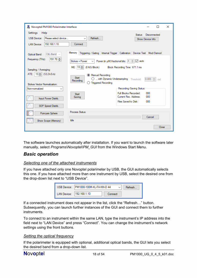
Selecting one of the attached instruments

If you have attached only one Novoptel polarimeter by USB, the GUI automatically selects

this one. If you have attached more than one instrument by USB, select the desired one from

the drop-down list next to “USB Device”.

If a connected instrument does not appear in the list, click the “Refresh…” button.

Subsequently, you can launch further instances of the GUI and connect them to further

instruments.

To connect to an instrument within the same LAN, type the instrument’s IP address into the

field next to “LAN Device” and press “Connect”. You can change the instrument’s network

settings using the front buttons.

Setting the optical frequency

If the polarimeter is equipped with optional, additional optical bands, the GUI lets you select

the desired band from a drop-down list.


Type the optical frequency in THz with up to two positions after decimal point into the field

besides Frequency and press Enter or tune the frequency with the up and down buttons.

Outside the calibrated frequency range, the polarimeter matrix will be extrapolated.

Measurements in the extrapolated range will be less accurate than in the calibrated range. If

a frequency in the extrapolated range is selected, a warning message will be displayed.

Setting the averaging time exponent (ATE)

Type any valid ATE value between 0 and 20 into the box and press Enter or adjust the ATE

with the up and down buttons. The resulting conversion rate is displayed at the right of the

box. Averaging time is 10 ns · 2ATE.

Selection of a normalization mode

Select the desired normalization mode from the drop-down list. See section Fundamental

PM1000 configuration for the definition of normalization modes.

Poincaré sphere display

With firmware 1.0.3.0 and GUI 1.0.7.0 or newer, the actual SOP samples can be displayed in

infinite persistence mode on the Poincaré sphere in the GUI at full sampling speed of 100

MHz. The display can be cleared by rotating the sphere with the mouse. The Poincaré

sphere window opens after pressing Poincare Sphere.

The sphere window can be resized by moving the window corners with the mouse. Power,

degree-of-polarization (DOP) and the three Stokes parameters are displayed as color bars

and text.


The orientation of the Poincaré sphere can be changed by moving the mouse on the sphere

with left button pressed. If the mouse is moved to the upper right corner, a menu will open.

The endless plotting of SOPs can be paused by clicking on the Resume/Pause button. The

sphere window can also be used to display SOP samples that have previously been stored in

the PM1000 internal memory, or loaded from files. This is done by selecting PM1000

memory or Data file instead of PM1000 live. After every window resize or sphere rotation, the

memory will be loaded again. The loading progress is displayed in the lower right corner.

If PER Measurement is activated, the GUI will analyze the current SOP trajectory. From the

maximum peripheral diameter of the trajectory, a PER value will be calculated and displayed.

Moving the trajectory to the center of the screen improves accuracy.

The user can calibrate the orientation of the sphere according to his needs. First, horizontal

or vertical polarization should be defined with the buttons Define SOP as Horiz. or Define

SOP as Vertical. This redefines the S1 axis, while the rotation about the S1 axis is still

undefined. This orientation can now be defined by the button Define SOP as Linear with a

linear input signal having an azimuth angle >0°, <90°. The more the azimuth angle differs

from 0° and 90°, the better. Reset to Defaults will restore factory settings. To store the new

orientation permanently, go to the Calibration tab on the main window and press Rewrite

PM1000 Flash Memory.

The power value displayed near the top, left of the Poincaré sphere, is averaged to suppress

power fluctuations. The averaging time can be adjusted by changing the value below the

label Power Averaging.


Oscilloscope plot

The stored Stokes parameters can also be displayed in an oscilloscope plot over time by

pressing Show Scope (Memory).

Four traces are being plotted in the new window: The three Stokes parameters S1-S3 plus

either power or DOP, whichever has been selected for memory recording, see section

Memory configuration. In the plot, the DOP will be normalized to 2, which means that a DOP

of 1 will appear in the middle of the y-range. The power curve is normalized to the maximum

value in the data set and refers to the y-axis on the right side of the plot. The maximum

power value is displayed in mW in the top right corner of the plot.

The plot can be zoomed in/out and shifted right and left. When more than one SOP event

has been recorded, the different events can be selected for plotting by up and down buttons:

The GUI oscilloscope plot allows to derive the SOP changing speed from the stored SOP

samples.

After selecting Speed from the drop-down list, the black curve in the plot will show the SOP

speed instead of Power or DOP. The SOP speed plot is normalized to its maximum, which is

displayed at the upper right of the plot. Since the SOP speed is calculated sample-to-sample,

it will contain a lot of noise when observing slow SOP changes with small ATE.


For deeper SOP analysis with other programs like Matlab, the data displayed in the

oscilloscope plot can be stored into a file on the computer by pressing Save data to file.

User Settings

Various settings can be set in the drop-down menu Settings of the GUI. Most of the settings

will be stored in the user’s application data directory, so that it will be remembered until the

GUI is uninstalled.

Configuration Files

The current configuration can also be saved to (“Export Configuration File…”) and loaded from (“Import Configuration File…”) files on disk. This includes basic settings such as optical frequency and averaging, but also the trigger configuration.

High-Sensitivity Mode

Optionally, the PM1000 is equipped with a high-sensitive mode, in which very weak signals

are measured with reduced noise at the cost of bandwidth. The GUI will display a message

once the PM1000 is in the high-sensitivity mode. The user can let the polarimeter switch

between the modes automatically (Auto) or force the polarimeter into the high-sensitivity

mode (ON) or into the normal mode (OFF). When measuring intensity-modulated signals, the

automatic mode selection can become unreliable and the user should determine one of the

modes himself.

Orientation of Stokes parameter S3

Two sign conventions exist for Stokes parameter S3. Transversal directions x and y form a

right-handed coordinate system either with propagation coordinate z or time t. Ellipse

handedness is defined when looking in direction of that axis z or t. For more information,


please refer to Application Note 3: “Mueller matrix measurement with PM1000 and

EPS1000”. Default factory setting is for x, y, z right-handed.

Auto-Averaging at low input power

If the optical signal is very weak, the polarimeter will reduce noise by averaging. If high

speed sampling is required and noise is tolerable, the user can disable the automatic

averaging here.

Non-normalized SOP Power Reference

In Non-normalized mode, Stokes vectors are normalized only with respect to a user-defined

power value, 1 mW by default. Here the power reference value can be defined in µW.

Log File Directory

By default, the log files are stored in the user’s application data directory. Hence they will be

deleted when the GUI is uninstalled. In the Settings menu, the user can set the log file

directory to Desktop instead

Data File Type

The memory data can be saved in binary or text file format. The binary format uses less disk

space and works faster, whereas the text format allows an easier processing of data with

external programs. The data type can be chosen in the menu strip Settings->Select Data File

Type.

Both file types start with an ASCII text header for additional data, e.g. sampling and

averaging time. Sample scripts for opening and plotting data in Matlab can be provided by

Novoptel. They are described at the end of this document.

Data File Timestamp

The timestamp in the data files can be referred to the local time or to UTC (Coordinated

Universal Time).

Auto-Save Files

During trigger-event recording, two types of files can be created:

- A single index file that includes a timestamp and the trigger source

- One data file with recorded pre- and post-trigger data for each trigger event.

Auto-Save Subdirectories

The number of files saved is only limited by disk space. Even if there is disk space available,

Windows sometimes blocks file creation in directories that already contain many ten

thousand files. If this setting is activated, the GUI will create a new directory at the beginning

of a measurement and every time the current directory is blocked.

Pre-Trigger Data Ratio

Selects the amount of pre-trigger data: 50% (default), 25% or 12.5%.


Memory configuration

The PM1000 internal memory allows to store up to 67 M SOP samples (2ME, between 210

and 226) at a rate of up to 100 MS/s. It is configured in the Memory tab of the main tab

control.


The block size of the memory is defined by a memory exponent (ME) between 10 and 26,

see section Fundamental PM1000 configuration. The memory block recording time, derived

from block size and averaging time, is displayed accordingly. There are 2(26-ME) memory

blocks.

Power or DOP recording

The memory stores 4 Stokes parameters at once. For the parameter S0, the GUI allows to

select either optical power or degree-of-polarization (DOP) for recording. If power is selected,

the unit of S0 will be µW. To increase accuracy, the 16 bit integer value can be shifted bitwise

to add some fractional bits before recording. If the option auto is selected, the number of

fractional bits will be selected automatically according to the current input power level.

Timestamps

When starting a recording, a 64 Bit reference timestamp will be written into the timestamp

registers, (addresses 512+300 to 512+303). The upper 37 Bit refer to the seconds elapsed

since 12:00:00 midnight, January 1, 0001 in the Gregorian calendar. The lower 27 Bits refer

to 10-ns-ticks elapsed in the current second.

The 64 Bit relative timestamps in the memory are referred to the reference timestamp. The

upper 8 Bits of the relative timestamp are the timestamp indicator (all “1”, which can be

excluded for the S0 Stokes parameter). The lower 56 Bit differ depending on recording

mode:

Trigger-event recording:

Bits 55 down to 53: Code for last trigger source.

Bits 52 down to 48: Reserved.


Bits 47 down to 0: Counter for elapsed Microseconds.

Dynamic undersampling:

Bits 55 down to 0: Counter for elapsed Nanoseconds. 56 Bits suffice for > 1 year

uninterrupted recording.

Manual recording

The polarimeter will just record a number of samples according to ME after the user presses

Start Recording, and then stop. The Memory will contain only SOP data, the timestamp

registers contain the timestamp of the SOP at address 0.

In all recording modes, the button Start Recording (which by starting became “Stop

Recording”) can be pressed a second time to stop the recording immediately.

Dynamic Undersampling

If the SOP is to be logged for a long time, the polarimeter can save memory space by

dynamically undersampling the data: An SOP is only recorded if one of the Stokes

parameters differ by a given threshold from the last saved SOP.

If the optical signal contains a lot of noise, the amount of recorded SOPs can still be very

high. To reduce the amount of data, increase either ATE or the Stokes parameter threshold.

In the latter case, the recording has to be stopped and started again for the changes to take

effect. In the memory, each SOP is followed by a timestamp with one exception: If the time

difference of two samples is 10 ns (which is only possible with ATE=0), the timestamp is

skipped. Also here, the memory timestamps are relative to the timestamp in the timestamp

register.

The memory block size in this mode is always 225 addresses, which should normally contain

224 SOPs and 224 relative timestamps. There are two such blocks available. When file saving

is active, the data from the block that is actively recording is already transferred to the PC

and written into the file up to the current recording address. When the polarimeter has

reached the end of the second block, it will overwrite the first block, but only if the GUI has

finished saving the data from the first block. The GUI will create a new file for each block, so

that a file usually contains not more than 224 SOPs. This limits the file size to about 256 MB

in binary format or about 800 MB in text format.

Triggered recording

The checkbox Triggered Recording enables the continuous, cyclic recording mode, which is

useful for detecting and recording rare SOP events. In this mode, each memory block is like

a ring memory in which the measurement process is repeated without interruption until a

trigger event occurs. This trigger event can be launched from an internal or external signal,

see next section. After a trigger event, a defined amount of post-trigger data is still recorded,

see Pre-Trigger Data Ratio in the previous section.


After the last of the post-trigger samples is recorded, the polarimeter will write a relative

timestamp into the memory both to mark the stop position in the block and to allow

calculation of the trigger event time. The timestamp in the memory is relative to the

timestamp in the timestamp registers.

After that, the recording will continue in the next memory block, expecting the next trigger

event. The maximum number of events n depends on the memory block size defined by ME:

n=226-ME. This means that at an ME of 26 (whole memory as one block), only one event is

recorded.

Saving the event data to files

After clicking on Start Saving and selecting a file name, the GUI downloads the event data

already while the next events are being recorded. Once the recording reaches the end of the

memory, the polarimeter will start over from the first block. If the events occur faster than the

data transfer of one block, the polarimeter will fill only as many block as are still available.

So, if downloading lags recording by the full memory size, trigger events or records will be

missed. The GUI will mark a block as available for the next recording after it has downloaded

its data. This way, the number of files is only limited by disk space, and also fast subsequent

events are recorded without having to wait for file transfer between the events.

If the recording has been stopped manually, the polarimeter will continue downloading the

rest of the events until the user clicks Stop Saving.

Triggering and gating

The Triggering / Gating tab of the GUI allows to enable triggering or gating of the memory

recording. Triggering means that the cyclic measurement process is stopped after recording

of post-trigger samples. Gating means that the recording process will be paused as long as

the gating signal is active.


The SOP event triggering / gating signal is the result of an internal Stokes vector

multiplication, see next section. The external triggering / gating signal is a LVCMOS33 (0 V /

+3.3 V) signal that is applied to the BNC connector at the rear panel of the instrument.

Retriggering

If “Rising edge” is selected, an SOP trigger is launched only in the moment the trigger

threshold is surpassed. If it is surpassed already before starting the recording, the trigger

launches only once eventually the trigger threshold is underrun and surpassed again. Until

then, the SOP event is not recorded. The same applies for SOP events that last longer than

the recording time of the post-trigger samples, where only the one block containing the

beginning of the event will be recorded. In both situations, activation of “Retrigger during long

SOP events” will launch additional triggers if a level higher than the trigger level is detected.

An SOP event lasting longer than the post-trigger recording time will then seamlessly

continue in the next recording block.

Internal trigger configuration

The internal trigger signals can be configured in the Internal Trigger tab of the GUI. There are

two basic internal trigger sources: SOP events and power events.

If the PM1000 is equipped with a digital feedback interface to the EPS1000 for SOP tracking,

the External SOP Reference serves as the target SOP for the tracking function.

SOP Event

The SOP event trigger signal is the length of a difference vector between the current and a

reference Stokes vector, normalized to a maximum of 1 (rather than the diameter 2 of the

Poincaré sphere). It is therefore a function of the angle δ between the two Stokes vectors:

Trigger signal = 0.5 ∙ | Scur-Sref |= sin(δ/2). For small δ it holds trigger signal δ/2.

For triggering, the trigger signal must surpass the trigger threshold. The trigger threshold can

be adjusted between 0 (trigger signal always high) and 1 (trigger signal always low) in steps

of 0.01.


At very low input power and small ATE, noise can lead to high calculated SOP changes and

create unwanted trigger edges. The trigger can be blocked if the power drops below an

adjustable power threshold (“Trigger Signal Power Thresh.”), which is 1 W by default.

Delayed measured SOP for reference

The reference Stokes vector can be chosen to be a copy of the permanently measured SOP

that has been delayed by a specified time. The delay time, see top of the figure above, is

specified by the number of clock cycles, tau, and an exponent for clock division, clkexp.

Based on an initial clock period of 10 ns, the delay Td can be calculated by Td = 10 ns ∙ tau ∙

2clkexp. By the angle δ and the time Td, a certain SOP changing speed δ/Td is specified. The

PM1000 will be triggered whenever the optical input signal surpasses this speed. In the

figure above, 0.2 rad within a delay time of 10 ns ∙ 3 ∙ 26 = 1920 ns means a SOP speed of

103.34 krad/s. Please note that for correct operation, the delay time should always be longer

than the averaging time (set by ATE).

External (user-specified) SOP for reference

It is possible to define an arbitrary Stokes vector as reference. To do so, enter three Stokes

parameters, separated by semicolons, in the text field of the drop-down box and press Set.

The Stokes vector will be normalized and transmitted to the polarimeter. One can also select

one of the predefined Stokes vectors from the drop-down list. Or, set the current measured

SOP as reference by pressing the button Set Cur. SOP.

Some applications may require the reference SOP to change over time, for example during a

laser sweep. This can be achieved by writing the desired parameters into a table memory,

see the chapter “Table memory”. Execution of the table is either triggered by a rising edge at

the BNC input or by writing to the corresponding register via USB, LAN or SPI. There are two

basic trigger modes, row or table:

Row Trigger Mode

In row trigger mode, the rows of the stored table are executed one-by-one upon a trigger

event. After the last table row, the counter starts over from the first table row.

Table Trigger Mode

In table trigger mode, the counter starts over from the first table entry upon every trigger.

Subsequent rows are executed after the dwell time delay specified in each row. After the last

table row, the row counter is halted until the next trigger event occurs.

Continuous Mode

In continuous mode, the counter is not halted after the last row but executed the table

continuously according to the dwell times specified in each row.

Power Event

The polarimeter can also trigger on input power events.

Gradient detection

This function allows triggering on power transients, for example if the power changes by

more than ±0.1 dB within 1 µs. Here the same delay time constant is used as for SOP

events. The power changing threshold can be given in dB in the GUI in steps of 0.01 and will

be written as a factor in the PM1000 registers (see register description). The internal error


signal changes from “0” to “1” when the power has increased or decreased by more than this

factor during the delay time constant.

Deviation detection

This function changes the internal trigger signal form “0” to “1” when the current input power

differs from a target power by more than a deviation tolerance, which acts as a threshold.

Target and deviation tolerance powers are given in W. One can set the current input power

as target power by pressing the button “Set Curr. Pow.” in the GUI.

If this signal is used for gating of SOP recording, “active low” has to be selected in the

Triggering/Gating tab in order to let the samples with power within the deviation tolerance

pass the gate.

Clock drift compensation

The Triggered Recording process may run for days or even for unlimited time collecting

events to be captured. During this, the internal microsecond-counter of the polarimeter will

drift away from the Windows PC clock. The latter may be synchronized to the true time by

appropriate measures. From polarimeter firmware 1.0.7.0 on, the GUI will read the internal

microsecond-counter at time of data downloading and compare it to the elapsed time derived

from the PC clock. It will calculate the deviation between the two clocks and create a second,

corrected timestamp for the captured data. In the created data files, the original timestamp is

either called Timestamp or TimestampUTC depending on chosen time format whereas the

corrected timestamp is either called Timestamp_Win or TimestampUTC_Win.

In Triggered Recording mode, both timestamps refer to the first SOP in the file. Timestamp or

TimestampUTC differs from file to file.

In Dynamic Undersampling mode, Timestamp or TimestampUTC refers to the time when

recording was activated and serves as a reference for the individual SOP timestamps.

Timestamp or TimestampUTC is the same in all data files of a common recording.

Timestamp_Win or TimestampUTC_Win is the time of the first SOP in a file, corrected by the


PC clock at time of downloading. All time corrections are applied only in integer

microseconds.

Time stamp calibration

Due to varying USB latency, all timestamps in the polarimeter have an additional common

error offset of up to a few milliseconds. If higher accuracy is required, the user can

additionally activate External signal triggering in Triggered Recording mode and provide an

event at the BNC port at a defined time. By analyzing the polarimeter clock timestamp in the

created file for this event, he can correct all other timestamps and reduce the error down to 1

microsecond. If events are provided at the BNC port from time to time and are captured by

External signal triggering, also polarimeter clock drift can be compensated with high

accuracy.

User calibration set

By default, the polarimeter uses the internal factory calibration set. Using the GUI a user

calibration set can be loaded to and from the polarimeter. It can also be stored in the

polarimeter’s permanent memory (Flash) by pressing the button “Rewrite Flash memory” to

be able to access it without GUI

The Flash rewriting function also permanently stores the current dark current values that can

be recalibrated using the front control buttons or by pressing the button Reset Dark Current.

Also stored are the user rotation matrixes from the recalibration function in the Poincaré

sphere window.


Device Test

If available, a Novoptel polarization scrambler/transformer (e.g. EPS1000 or EPX1000) can

be controlled by the GUI to measure polarization dependent loss (PDL) and the Mueller

matrix of a connected device under test or simply align the scrambler/transformer output

SOP to a specified vector.

Optional Optical Switches

If the polarimeter is equipped with one or two optical switches, they can be operated from the

GUI.

PDL by Extinction Method

If PDL is measured by Extinction Method, the polarization scrambler/transformer is driven to

obtain the polarization states where minimum and maximum transmissions are reached.

From minimum and maximum transmission, PDL can be calculated.

Starting at “0”, all 16 electrode voltages are modified subsequently. After measuring the

optical power at maximum and minimum transmission, the calculated PDL will displayed.


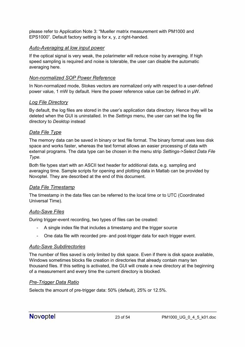
Mueller matrix measurement

PDL can also calculated from the Mueller matrix of a DUT. To measure the Mueller matrix of

a DUT, first a minimum of 4 voltage sets that lead to a predefined polarization states have to

be found. Examples for most suitable polarization sets are the corners of tetrahedrons,

diamonds, cubes and other polyhedrons. The GUI allows to choose between 1, 3, 4, 6, 8, 14

and 20 polarization states, where “4” corresponds to 4 corners of a tetrahedron, “6”

corresponds to the 6 normal vectors on the surface of a cube, “8” corresponds to the 8

corners of this cube, “14” is a combination of the two, and “20” corresponds to the corners of

a dodecahedron. The selection of “1” or “3” is not suitable for measuring the Mueller matrix.

The EPS1000 will cyclically apply the selected number of SOPs to the DUT, with a dwell time

in each state between 1.28 µs and 1 ms. In the above configuration, one Mueller matrix takes

14 times 1 ms, so 14 ms. If one needs to shorten the measurement time, for example during

a fast laser sweep, one can reduce the number of SOPs and select a shorter dwell time. The

fastest possible Mueller measurement takes 4 times 1.28 µs, so 5.12 µs.

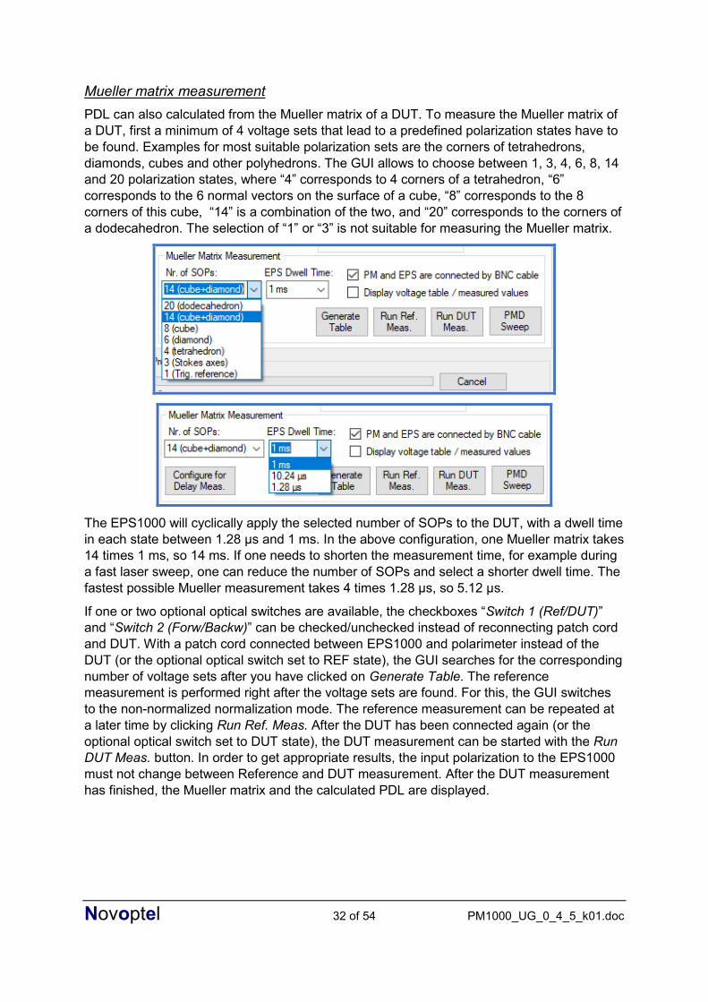
If one or two optional optical switches are available, the checkboxes “Switch 1 (Ref/DUT)”

and “Switch 2 (Forw/Backw)” can be checked/unchecked instead of reconnecting patch cord

and DUT. With a patch cord connected between EPS1000 and polarimeter instead of the

DUT (or the optional optical switch set to REF state), the GUI searches for the corresponding

number of voltage sets after you have clicked on Generate Table. The reference

measurement is performed right after the voltage sets are found. For this, the GUI switches

to the non-normalized normalization mode. The reference measurement can be repeated at

a later time by clicking Run Ref. Meas. After the DUT has been connected again (or the

optional optical switch set to DUT state), the DUT measurement can be started with the Run

DUT Meas. button. In order to get appropriate results, the input polarization to the EPS1000

must not change between Reference and DUT measurement. After the DUT measurement

has finished, the Mueller matrix and the calculated PDL are displayed.


Aligning the scrambler output to specific polarizations

If “3 (Stokes axes)” is selected from the dropdown list of target SOPs, the GUI will create a

voltage table which switches between horizontal ([1 0 0]), vertical ([0 1 0]) and right-circular

([0 0 1]) polarization. If “1 (Trig. Reference)” is selected, the GUI will align the polarization to

the reference SOP defined in the “Internal Trigger” / “SOP Event” tab. Apart from selecting

one SOP from the dropdown list, any vector can be typed into the textbox in the format “0.00;

0.00; 0.00”.

If you want to keep the generated voltage table for later usage, press “Disconnect” in the

“Device Test” tab of the PM1000 GUI to disconnect from the scrambler. Then open the

EPS1000 GUI, connect to the scrambler and click “Save File” in the “Synchronous/Triggered

Scrambling” tab of the EPS1000 GUI. This way one can create several files that allow

switching to desired polarizations by loading the corresponding file into the EPS1000 GUI.

Please not that these files are only valid as long as the input polarization to the scrambler is

preserved.

Synchronizing Polarimeter and Scrambler

If PM1000 and EPS1000 are connected by a BNC cable, SOP switching and SOP recording

can be synchronized. In this case, the dwell time at each input SOP is reduced from about

1 s to 1 ms, which dramatically reduces measurement time.

Delaying the external trigger signal input:

Caused by internal processing, Stokes parameter signals reach the PM1000 memory with a

delay of about 0.8 µs. This means that if polarization changes and external trigger signal

occur simultaneously, the source of the recorded sample lies 0.8 us in the past. The PM1000

can compensate the Stokes parameter time lag by delaying the trigger signal internally. If


synchronism is required, the user should set TAU=80 and CLKEXP=0 in the Triggering /

Gating tab to achieve a trigger signal delay of 0.8 us.

During Mueller matrix measurement with synchronized PM1000 and EPS1000 in contrast,

the Stokes parameter time lag is helpful: As the EPS1000 will indicate a polarization change

at the beginning of each cycle with a rising edge of the trigger signal, the PM1000 will store a

sample from the time the polarization was stable, 0.8 us in the past. Any delay of the DUT

will be added to the Stokes parameter time lag. Very long DUT delays or very short cycles

can cause the PM1000 to sample in an unstable region of a cycle, e.g. in the first half of the

cycle. In this case the trigger should be delayed to compensate the delay of the DUT.

Since firmware 1.0.3.1, the delay can be defined by TAU * 2CLKEXP * 10 ns, where TAU is

between 13 and 524 and CLKEXP is between 0 and 15. The minimum value 13 of TAU is

caused by a fundamental processing delay of the trigger signal. CLKEXP causes an

undersampling of the trigger input. The undersampling can increase the uncertainty of the

sampling point within the cycle. Hence it is recommended to make use of the full range of

TAU and let CLKEXP be as small as possible.

Determining the DUT delay with synchronized PM1000 and EPS1000:

The delay of the DUT can be determined by recording a polarization event synchronous to

the external trigger input using the trigger event recording function of the PM1000. The

button Configure for Delay Meas. in the Device Test tab will load a suitable voltage table with

100 ms cycle time to the EPS1000. In the Memory tab, enable Trigger-Event Recording,

press Start Recording and open the oscilloscope window after the measurement has been

completed. By using a suitable ATE value and the zoom function of the oscilloscope view,

the time difference between trigger event (the center of the figure as long as not shifted) and

SOP event can be determined. Change the delay in the Triggering / Gating tab and repeat

the measurement until the DUT delay is compensated. It is recommended to leave a small

(positive) safety margin between trigger and SOP event, for example 0.5 µs at a cycle time of

1 ms. The adjusted trigger delay will be applied during the DUT measurement of a Mueller

matrix measurement. The adjusted values will be ignored in the reference measurement

since most commonly a patch cord is used as the DUT and the delay will be close to zero.


Wavelength Sweep

The polarimeter GUI can measure, store and evaluate Mueller matrices obtained during a

wavelength sweep and calculate the differential group delay (DGD) of the device under test

(DUT). Since the sweep consist of discrete frequency steps, measurement range depends

on step size. With 50 GHz frequency steps, maximum unambiguous DGD measurement is

limited (by Nyquist’s theorem) to 1/(2 * 50 GHz) = 10 ps. If larger DGD is to be measured,

smaller frequency steps must be chosen. On the other side of the range, with a maximum

frequency difference of 88*50 GHz = 4.4 THz, mean DGDs of 12 fs have been measured

with a standard deviation of ≤ 3 fs in experiments.


Sweep with Novoptel LU1000:

If a Novoptel laser unit LU1000 is connected by USB to the same PC, it can be controlled by

the polarimeter GUI during the wavelength sweep. After the GUI connects to the LU1000, it

displays the laser module capabilities and sets the sweep settings to cover the maximum

possible wavelength range. The pause time (here: 50 ms) during the channel switching also

depends on the laser module type and has to be checked against the laser module data

sheet by the user.

There are two possibilities to perform the sweep(s):

a) One sweep of the reference path (button Run Ref. Sweep), then switching to the DUT

path with the switch control on the polarimeter main window, then one sweep of the

DUT path (button Run DUT Sweep). One reference sweep can be used for several

subsequent DUT sweeps.

b) One combined sweep, during which the optical switch is automatically toggled at each

frequency to measure both reference and DUT. This means more frequent switching.

Switch lifetime is defined by the manufacturer as >107 cycles.

Saving measurement data:

After the DUT sweep (or the combined sweep in above case b)) the calculated DGD value

will be displayed. For further analysis, the obtained data can be saved to a text file in Matlab

format. The saved data contains

- current laser frequency,

- Mueller matrix,

- Mueller-Jones matrix,

- Jones matrix,

- mean loss and

- PDL

for each wavelength during the sweep.

Sweep with other laser, controlled by user:

If no LU1000 is available, the sweep can be performed by any other laser that meets one of

the following conditions a) or b) below. Start frequency/wavelength, step size and number of

frequencies/wavelengths have to be defined before the sweep.

a) While switching from one channel to the next, the output power must drop

significantly (by >10 dB) for at least 2 Milliseconds. This way, the GUI can indicate a

number of laser pulses corresponding to the different wavelengths in the measured

data. If the number of detected pulses differs from the set value, a warning will be

displayed after the measurement. The user must set the laser to a channel >1 before

the sweep, so that the switching to channel 1 upon starting the sweep can be

recognized by the associated intensity dip. The width of the laser pulses must exceed

the measuring time for one Mueller matrix. E.g. if the Nr. of SOPs for each

measurement is set to 14 (cube+diamond) with dwell time 1 ms in the main window,

each Mueller matrix measurement takes 14 * 1 ms, and so the laser pulse width

should be >14 ms + intensity dip time. To start the reference measurement, click Ext.

Ref Sweep. Then manually start the sweep of the laser. After the laser finished the

sweep, stop the measurement with the cancel button at the bottom of the polarimeter

main window.


b) The laser provides a rising edge in a LVCMOS33 trigger signal after each sweep

step. Ensure that the laser step time exceeds the Mueller matrix measurement time. To start the reference measurement, click Ext. Ref Sweep. Then manually start the

sweep of the laser. The progress of the measurement will be shown on the progress

bar in the main window. If no progress is reported, check BNC connection between

laser and PM1000. After the specified number of Mueller matrixes have been

measured, the process will stop.

To measure the DUT, switch the paths and repeat above steps except that you now click Ext.

DUT Sweep. Saving data and using calibration files is the same as with LU1000. Combined

sweeps of Ref. + DUT are not possible here.

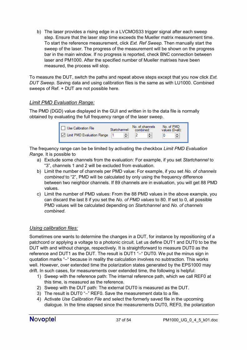
Limit PMD Evaluation Range:

The PMD (DGD) value displayed in the GUI and written in to the data file is normally

obtained by evaluating the full frequency range of the laser sweep.

The frequency range can be be limited by activating the checkbox Limit PMD Evaluation

Range. It is possible to

a) Exclude some channels from the evaluation: For example, if you set Startchannel to

“3”, channels 1 and 2 will be excluded from evaluation.

b) Limit the number of channels per PMD value: For example, if you set No. of channels

combined to “2”, PMD will be calculated by only using the frequency difference

between two neighbor channels. If 89 channels are in evaluation, you will get 88 PMD

values.

c) Limit the number of PMD values: From the 88 PMD values in the above example, you

can discard the last 8 if you set the No. of PMD values to 80. If set to 0, all possible

PMD values will be calculated depending on Startchannel and No. of channels

combined.

Using calibration files:

Sometimes one wants to determine the changes in a DUT, for instance by repositioning of a

patchcord or applying a voltage to a photonic circuit. Let us define DUT1 and DUT0 to be the

DUT with and without change, respectively. It is straightforward to measure DUT0 as the

reference and DUT1 as the DUT. The result is DUT1 “–“ DUT0. We put the minus sign in

quotation marks “–“ because in reality the calculation involves no subtraction. This works

well. However, over extended time the polarization states generated by the EPS1000 may

drift. In such cases, for measurements over extended time, the following is helpful:

1) Sweep with the reference path: The internal reference path, which we call REF0 at

this time, is measured as the reference.

2) Sweep with the DUT path: The external DUT0 is measured as the DUT.

3) The result is DUT0 “–” REF0. Save the measurement data to a file.

4) Activate Use Calibration File and select the formerly saved file in the upcoming

dialogue. In the time elapsed since the measurements DUT0, REF0, the polarization


states of the EPS1000 may have drifted, or may have been searched anew. This

does not matter significantly.

5) Sweep with the reference path: The internal reference path, which we call REF1 at

this time, is measured as the reference.

6) Sweep with the DUT path: The external DUT1 is measured as the DUT.

7) The displayed result will be (DUT1 “–“ REF1) “–“ (DUT0 “–“ REF0) = (DUT1 ”–”

DUT0) ”–” (REF1 ”–” REF0)”, i.e., DUT change “minus” reference change.

The measurements can be verified with, say, a patchcord as DUT. If it is left unchanged all

the time, DUT1 “–“ DUT0 and (DUT1 “–“ REF1) “–“ (DUT0 “–“ REF0) both yield a Mueller

matrix very close to identity. But if a lot of time has elapsed between measurements DUT0,

DUT1, then (DUT1 “–“ REF1) “–“ (DUT0 “–“ REF0) (with REF0 measured together with

DUT0, and REF1 together with DUT1) will generally be closer to the identity matrix than

DUT1 “–“ DUT0.


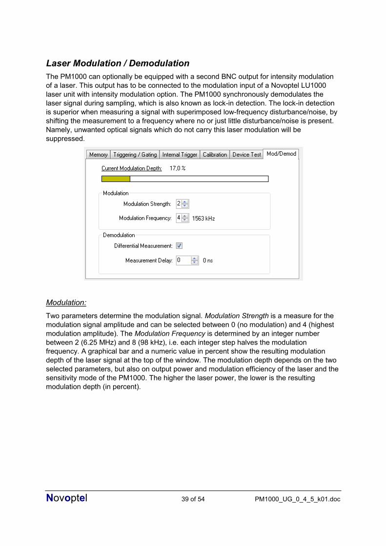
Laser Modulation / Demodulation

The PM1000 can optionally be equipped with a second BNC output for intensity modulation

of a laser. This output has to be connected to the modulation input of a Novoptel LU1000

laser unit with intensity modulation option. The PM1000 synchronously demodulates the

laser signal during sampling, which is also known as lock-in detection. The lock-in detection

is superior when measuring a signal with superimposed low-frequency disturbance/noise, by

shifting the measurement to a frequency where no or just little disturbance/noise is present.

Namely, unwanted optical signals which do not carry this laser modulation will be

suppressed.

Modulation:

Two parameters determine the modulation signal. Modulation Strength is a measure for the

modulation signal amplitude and can be selected between 0 (no modulation) and 4 (highest

modulation amplitude). The Modulation Frequency is determined by an integer number

between 2 (6.25 MHz) and 8 (98 kHz), i.e. each integer step halves the modulation

frequency. A graphical bar and a numeric value in percent show the resulting modulation

depth of the laser signal at the top of the window. The modulation depth depends on the two

selected parameters, but also on output power and modulation efficiency of the laser and the

sensitivity mode of the PM1000. The higher the laser power, the lower is the resulting

modulation depth (in percent).


Fig. 2: Modulation depth depending on laser output power, modulation strength = 4

It is recommended to operate with modulation depths of about 50%. Larger modulation

depths can cause mode hops or slow response. Current modulation (in mA) and optical

power modulation (in mW) inside the LU1000 is proportional to modulation strength. So, for a

given modulation strength, modulation depth is low at high mean powers and high at low

mean powers. Furthermore, associated FM is on the order of 100 MHz and decreases with

increasing modulation frequency.

Fig. 3 shows that with an output power of about +13 dBm, a 50% modulation depth is

reached for modulation frequencies 98 kHz ... 1563 kHz. This is the recommended usage. In

the high-sensitivity range with limited bandwidth, response is significantly reduced already at

3125 kHz. In the normal mode response is significantly reduced only at 6250 kHz, due to the

laser’s modulation bandwidth.

Demodulation:

The checkbox Differential Measurement enables the demodulation. When activated, the

signal is averaged over quarters of the modulation period. The PM1000 takes the signal

difference between 2nd and 4th quarter of the modulation period to generate the

demodulated measurement signal. Please not that in this mode, the stored and displayed

signal power depends the modulation depth and can therefore be lower than the actual or

mean input power.

Successful demodulation depends on the signal delay between the source modulation and

the optical input signal of the PM1000. When measuring Mueller matrices or PDL, also the

DUT can add extra delay. This gets more important at higher modulation frequencies. The

user can take into account increased signal delay by setting the additional Measurement

Delay in steps of 10 ns until the current modulation depth reaches a maximum. For Mueller

matrices or PDL measurements, the user may have to set different delays for reference and

DUT measurement.


Input Power Histograms

The polarimeter can accumulate the actual input power value in a histogram. The GUI

configures, reads and displays the histogram.

If desired, the user can switch to “Power deviation per time”, where only the difference

between the actual power value and a delayed power value is put into the histogram. The

delay time can is determined by the values tau and clkexp and can be calculated by Td = 10

ns ∙ tau ∙ 2clkexp.

A new value is put into the histogram every 20 ns if clkexp is 0 or 1. For other values of

clkexp, the period is 10 ns ∙ 2clkexp.

The histogram data can be saved to a text file.

SOP Speed Histograms

The polarimeter can calculate the momentary SOP speed and accumulate the values in a

histogram. For this purpose, the current SOP is compared with a delayed copy of an earlier

SOP. Again, the delay Td is calculated by Td = 10 ns ∙ tau ∙ 2clkexp.

If a large SOP arc exceeds the histogram range, it is put into the last histogram bin with

number 1024. If bin number 1024 is filled during a measurement, the user should decrease

the delay time so that the future SOP arcs become smaller and match the histogram range.

A new value is put into the histogram every 20 ns if clkexp is 0 or 1. For other values of

clkexp, the period is 10 ns ∙ 2clkexp.

The histogram data can be saved to a text file.

In the logarithmic plot, the y-axis gives the count readings of the histogram bins. In the linear

plot, the y-axis is normalized to the sum of all count readings.



Using Matlab to analyze stored data

As described in the sections above, the GUI allows storing the measured data in form of text

or binary files. These files can be opened for further investigation by Matlab or other

programs in an easy way. Since version 2.0.0.0 of the GUI, timestamps are included in the

files for each SOP.

The files start with a header that contains the measurement meta data. The header of text

files is formatted in such a way that it can directly be evaluated by Matlab after the hash (“#”)

signs are removed:

# Timestamp='2018.08.21 09:35:45.385';

# ATE=7;

# SamplePeriod_ns=1280;

# ME=10;

# Data1Name='Power';

# PowerLeftShift=4;

# Normalization=1;

# NonNormPowRef=1000;

# TriggerGatingReg=1;

# CyclicRecording=1;

# PreTriggerSamples=0.125;

# TriggerSource='SOP 19.56 krad/s';

# SOPTriggerConfiguration=799;

# SOPTriggerThreshold=655;

# SOPTriggerPowerThreshold=1;

# POWTriggerReference=1000;

# POWTriggerThreshold=100;

In binary files, the length of the header is given by the variable headerlength, which itself

stands at the beginning of the header. It is at least 256. This means that the first 256 bytes of

the file (or more, if headerlength is larger) represent text in ASCII format which should be

evaluated to get the measurement metadata. The measurement data starts after the header

at byte 256 (if header bytes are counted from 0 to 255), i.e. byte 257 in total. The variable

Timestamp is a timestamp at the last sample of the measurement data. This time counting

inside the PM1000 is synchronized with the host PC at the beginning of the recording with an

uncertainty of about 1 ms. This timestamp can be used to calculate the trigger moment when

the duration of post-trigger data sampling is subtracted. ATE, ME and Normalization refer to

the selected settings of the same name. SamplePeriod_ns is the sample period in

nanoseconds, derived from ATE. Data1Name is either “Power” or “DOP”, depending on the

data selection for the Stokes parameter S0. When “Power” is selected, the value

PowerLeftShift determines the amount of fractional bits in the data of S0. For example, if

“PowerLeftShift=4”, a value S0 of 17520 in the file corresponds to an input power of

17520*2-4 = 1095 Microwatts.

In the “Non-normalization” mode, the Stokes parameters S1 to S3 are only normalized to the

specified power reference, given in the variable NonNormPowRef.

TriggerGatingReg is the content of register (512+92) which defines the triggering and gating

conditions.

When the PM1000 is in cyclic (triggered) recording mode (CyclicRecording=1),

PreTriggerSamples states the relative amount of pre-trigger samples in the data.

TriggerSource reveals the actual trigger event, either “SOP”, “POW” or “EXT”,

notwithstanding the fact that more than one trigger source may have been configured in the

tab “Triggering / Gating” . “POW” and “EXT” are followed by the trigger threshold.


TriggerConfiguration refers to the trigger signal configuration register (512+86) and

TriggerThreshold is the value of the trigger threshold register (512+91).

SOPTriggerPowerThreshold is the power in Microwatts, under which the SOP trigger would

be blocked.

POWTriggerReference and POWTriggerThreshold give the power reference and power

threshold for the power event trigger signal.

In contrast to binary files, the byte length of the header in text files is not specified. Hence the

variable headerlength is missing. Instead, all lines of the header begin with a hash sign to

distinguish header from subsequent measurement data.

The measurement data in text files are comma-separated values that also allow opening the

file in Excel for instance. The binary files cannot be opened by Excel. If files were saved in

binary format by mistake, they can be opened in the GUI’s oscilloscope window and saved

again, this time in text format.

The following Matlab or GNU Octave (www.octave.org) function pm1000plot.m opens a file

and plots the contained data. This function is available at

https://www.novoptel.de/Home/Downloads/pm1000plot.m or

https://www.novoptel.eu/Home/Downloads/pm1000plot.m. Since standard browsers open

.m files as text files, simply save the file pm1000plot.m from within the browser.

% This is to plot the Stokes parameters loaded from a Novoptel PM1000 polarimeter

% supports GUI version 2.0.0.0, with Timestamps

% Copyright 2020 Benjamin Koch, Novoptel GmbH

% Usage: pm1000plot(filename, withtimestamps); % filename can for instance be 'myrecord.txt' (text file) or 'myrecord.bin' (binary file). % For GUI >=2.0.0.0, firmware >=1.0.6.0, the records contain timestamps. % To accomodate this, withtimestamps is chosen as 1 or, if dropped, is chosen as 1 by default. % Examples: pm1000plot('myrecord.txt'); pm1000plot('myrecord.bin'); % pm1000plot('myrecord.txt',1); pm1000plot('myrecord.bin',1); % For GUI <2.0.0.0, there are no timestamps, and one sets withtimestamps as 0. % Examples: pm1000plot('myrecord.txt',0); pm1000plot('myrecord.bin',0);

function pm1000plot(filename, withtimestamps)

if (nargin<2) || isempty(withtimestamps) withtimestamps=1; end

% open the data file

FID=fopen(filename);

if sum(filename(end-3:end)=='.bin')==4, % this is a binary file

% get the header length (mimimum 256 bytes)

C=fread(FID, 256, 'uint8');

headerstrings=strsplit(char(transpose(C)), char(13));

try eval(char(headerstrings(1)))

catch err

disp(sprintf('ERROR: Unknown command: %s', char(headerstrings(1))));

pause

end

% get the full header with meta data

fseek(FID, 0, 'bof');

C=fread(FID, headerlength, 'uint8');

headerstrings=strsplit(char(transpose(C)), char(13));

size_headerstrings=size(headerstrings);

nlines=size_headerstrings(2);

% load information from meta data

if nlines>2,

for ii=2:nlines-1

https://www.novoptel.de/Home/Downloads/pm1000plot.m

https://www.novoptel.eu/Home/Downloads/pm1000plot.m


try eval(char(headerstrings(ii)))

catch err

disp(sprintf('ERROR: Unknown command: %s', char(headerstrings(ii))));

pause

end

end;

end;

% get the data after the header

fseek(FID, headerlength, 'bof');

C=fread(FID, 'uint16');

if withtimestamps,

% get the timestamps and stokes parameters

TS_N = reshape(C, 8, floor(length(C)/8));

% get the timestamps, referred to the first sample

Timestamp_ns = uint64(TS_N(4,:)*2^48) + uint64(TS_N(3,:)*2^32) ...

+ uint64(TS_N(2,:)*2^16 )+ uint64(TS_N(1,:));

Timestamp_ns = Timestamp_ns - Timestamp_ns(1);

% restore the Stokes parameters

N=TS_N(5:8,:);

else

N = reshape(C, 4, floor(length(C)/4));

Timestamp_ns = (1:length(N))*SamplePeriod_ns;

end;

else % this is text file

% get the meta data

C=textscan(FID, '#%s', 'Delimiter', '@');

% load information from meta data

if length(C{1})>0,

for ii = 1:length(C{1}),

try eval(C{1}{ii})

catch err

disp(sprintf('ERROR: Unknown command: %s', C{1}{ii}));

end

end

end

if withtimestamps,

% get the timestamps and stokes parameters

NN=textscan(FID,'%f %f %f %f %f','Delimiter',',');

clear Timestamp_ns;

Timestamp_ns(1,:)=NN{1};


clear N

for ii=2:5,

N(ii-1,:)=NN{ii};

end;

else

% get the stokes parameters

NN=textscan(FID,'%f %f %f %f','Delimiter',',');


clear N

for ii=1:4,

N(ii,:)=NN{ii};

end;

Timestamp_ns = (1:length(N))*SamplePeriod_ns;

end

end;

% close the data file

fclose(FID);


% remove offset from Stokes parameters 1..3

N(2:4,:)=N(2:4,:)-2^15;

S=N/2^15;

% plot the data

figure;

x=Timestamp_ns; %X-axis in Nanoseconds

plot(x, S(1,:), '.:k', x, S(2,:), '.:r', x, S(3,:), '.:b', ...

x, S(4,:), '.:g');

legend(Data1Name, 'Stokes 1', 'Stokes 2', 'Stokes 3');

xlabel('Nanoseconds');

grid on;


Operation of the instrument using register access

The polarimeter is controlled by reading from and writing to internal control registers, see

chapter “register description”.

Access the USB driver

The USB driver has to be installed on your system and the instrument needs to be connected

using a USB cable.

Support for Matlab

Matlab needs a header file like ftd2xx.h from FTDI to access the USB 2.0 driver directly.

Novoptel provides the header version matftd2xx.h, in which the data types are modified to

become compatible with current Matlab versions.

You will find help about communicating to a driver at

http://www.mathworks.com/help/techdoc/ref/loadlibrary.html

The different functions of the driver can be seen from the header file. Information about each

function is provided at http://www.ftdichip.com/Support/Knowledgebase/index.html

To avoid accessing the driver with Matlab directly, Novoptel provides precompiled MEX files

for basic read and write functions. Examples of Matlab communication scripts are included in

Matlab_USB_Support_Files.zip, which can be downloaded from

https://www.novoptel.de/Home/Downloads_en.php and

https://www.novoptel.eu/Home/Downloads_en.php.

USB 2.0 Settings

The following settings have to be applied within Matlab (or other programs) to enable USB

communication:

Baud Rate 230400 baud

Word Length 8 Bits

Stop Bits 1 Bit

Parity 0 Bit

To speed up sequential read and write operations, we further recommend the following

setting:

USB Latency Timer 2 ms

USB 2.0 Transfer protocol

The instrument is controlled by reading from and writing to USB registers. The register

address line is 12 bits wide, while each register stores 16 bits. All communication is initiated

by the USB host, e.g. the Matlab program.

Writing to a register uses a 9 byte data packet. Each byte represents an ASCII-coded

character. The packet starts with the ASCII-character “W” and ends with the ASCII-code for

carriage return.

http://www.mathworks.com/help/techdoc/ref/loadlibrary.html

http://www.ftdichip.com/Support/Knowledgebase/index.html

https://www.novoptel.de/Home/Downloads_en.php

https://www.novoptel.eu/Home/Downloads_en.php


Send write data packet

„W“ A(2) A(1) A(0) D(3) D(2) D(1) D(0) ^CR

The 12 bit register address A is sent using 3 bytes, each containing the ASCII-character of

the hexadecimal numbers 0 to F which represents the 4 bit nibble. The character of the most

significant nibble is sent first. The 16 bit data, which should be written into the register, is

sent with 4 bytes using the same coding as the register address.

Reading data from a register requires the host to send a request data packet to the

instrument. The packet starts with the ASCII-character “R”, followed by the register address

coded the same way as in write data packets.

Send request data packet

„R“ A(2) A(1) A(0) „0“ „0“ „0“ „0“ ^CR

After receiving the request data packet, the instrument sends the requested data packet to

the host:

D(3) D(2) D(1) D(0) CR

Burst transfer

To increase transfer speed, consecutive addresses of an internal memory can be transferred at once. Additional packets are defined for this purpose:

Send Set burst address register packet

„X“ „0“ „0“ „0“ D(3) D(2) D(1) D(0) ^CR

The data D is the address of the register that will be incremented during burst transfer. In

most cases, this register will represent the read address of a memory.

Send Set start value packet

„X“ „0“ „0“ „1“ D(3) D(2) D(1) D(0) ^CR

The data D is the start value of the counting.

Send Set stop value packet

„X“ „0“ „0“ „2“ D(3) D(2) D(1) D(0) ^CR

The data D is the stop value of the counting

Send Set read address packet

„X“ „0“ „0“ „3“ D(3) D(2) D(1) D(0) ^CR


The data D is the address of a register that contains the data to be sent during burst transfer.

In most cases, this register will represent the data output of a memory. After sending this

packet, burst transfer will start. Beginning with the start value, the address register will be

incremented until it reaches the stop value. After every step, the data appearing in the read

address register will be transferred to the host.

SDRAM data transfer

To increase transmission speed when reading from the SDRAM of the PM1000, parts of the

SDRAM can be transferred in a single packet. The SDRAM part is defined by the start

address and the number of addresses to be transferred. Since the start address is 26 bit

wide, it requires 2 registers for definition. One SDRAM address contains one SOP (4 Stokes

parameters * 16 bit = 64 bit). Since the buffer size is 2^16 bytes, the packet size is limited to

2^13 SOPs. The data transfer sequence is as follows:

- write lower 16 bits of start address into register number 512+105

- write upper 10 bits of start address into register number 512+106

- write number of addresses to be transferred into register number 512+107

- write “39293” into register number 512+104 (this triggers the transfer)

- wait for buffer to be filled, then read the buffer

USB 3.0 Transfer protocol

The protocol of the USB 3.0 interface differs from USB 2.0. CRC words and ACK packets

ensure correct data transfer. The word size is 16 bit instead of 8 bit.

Write data packet

Writing to a register via USB 3.0 requires a 4 word (1 word = 16 bit) data packet. The packet

starts again with the ASCII-code 0x57 (for “W”), but here as a 16 bit word instead of a byte.

„W“ A(11..0) D(15..0) CRC

The 12 bit register address is sent in the second word, followed by the 16 bit register data in

another word. The packet is completed by a cyclic redundancy check (CRC) word. The CRC

value can be calculated by the following c-code lines, assuming the array data_p contains

the write data packet:

crc = 0xFFFF;

length = 3;

while (length--)

{

crc = (crc<<1) | (crc>>15); // cyclic shift of crc

crc ^= *data_p++; // xor with data

}

After the PM1000 has received the write data packet, it sends an acknowledgement (ACK)

packet:

CRC_OK CMD A(11..0) D(15..0)

At least the first word of the ACK packet should be checked by the transmission script. If

CRC_OK equals 52428, the PM1000 has received a packet with correct CRC word. The rest


of the packet are command (CMD, = “W” in this case), register address and register data as

in the write data packet sent to the PM1000.

Request data packet

„R“ A(11..0) 0 CRC


the host:

FIFO LENGTH PM_CRC D(15..0) FIFO_CRC

FIFO_LENGTH and FIFO_CRC are for SDRAM data transfer and can be ignored here.

D(15..0) is the data read from the register. PM_CRC is the CRC calculated from the request

packet and the register data word. It can be calculated with the following c-code lines:

crc = crc_req; // crc as sent in the request packet

crc = (crc<<1) | (crc>>15); // cyclic shift of crc

crc ^= data; // xor with received data word

SDRAM data transfer

The USB 3.0 interface also supports SDRAM data transfer. The buffer sizes is smaller (4096

bytes), which limits the number of SOPs/addresses per packet to 512. Up to the triggering of

the data transfer (“39293” to register 512+104), the packet sequence is the same as in the

USB 2.0 case. After the transfer triggering, one must continuously read an arbitrary register

and check the FIFO_LENGTH packet until its value reaches the requested number of SOPs.

Then, the interface has to be switched into the FIFO mode by the following packet:

„F“ 0 0 CRC

This packet will not be acknowledged. Instead, the requested number of SOPs can now be

read from the interface. The SOP data can be verified by calculating the CRC over the

complete packet and compare it with FIFO_CRC of the last request data packet.


TCP/IP (LAN) Communication

The user can set the IP address, gateway and subnet mask via the front buttons. After the

next power-up, the PM1000 will open a TCP/IP socket using the entered settings and wait for

a connection.

TCP/IP Settings

Port: 5025

Input buffer: 16384 Bytes

Write data packet

In contrast to USB 2.0 communication, writing to a register via TCP/IP requires only a 5 byte

data packet. The packet starts with the ASCII-code 0x57 (for “W”).

„W“ A(11..8) A(7..0) D(15..8) D(7..0)

The 12 bit register address is sent first in two bytes, followed by the 16 bit register data in

another two bytes.

Reading data over TCP/IP requires the program to send a request data packet of 3 bytes to

the instrument. The packet starts with the ASCII-code 0x52 (for “R”), followed by the register

address coded the same way as in write data packets.

Request data packet

„R“ A(11..8) A(7..0)


the host:

D(1) D(0)

SDRAM data transfer

The SDRAM data transfer sequence is identical to the USB 2.0 case, except for the

following:

- The buffer size is 16384 bytes

- The trigger code is “39294” instead of “39293”


SPI Communication

All internal registers can also accessed by SPI. The SPI interface allows communication with

much lower latency than USB. The SPI connector at the backside of the device provides the

following connection:

Connector

notch

SDI GND CS

SDO GND SDCK

Transmission starts with falling edge of CS and ends with rising edge of CS. After falling

edge of CS, the command is transmitted. SDI is sampled with rising edge of SCK. Maximum

SCK frequency is 500 kHz. Command and data word length is 16 bit each. MSB of command

and data word is sent first, LSB last. If a valid register read (RDREG) command is received,

the SDO output register shifts with falling edge of SCK to transmit the requested data word.

Otherwise SDO remains in high impedance state. Data transfer to the device continues

directly after transmitting a register write (WRREG) command.

Serial interface (SPI) commands

Command Code Data Function

RDREG 0XXXh OUT Read register XXXh (see section Register description)

WRREG 1XXXh IN Write register XXXh (see section Register description)

Serial interface (SPI) timing

Fig. 3: Timing of SPI port.

Symbol Description Min Max Units

TCSCK CS low to SDCK high 120 – ns

TCKCS SDCK low to CS high 120 – ns

TSDCKL SDCKL low time 1 – µs

TSDCKH SDCKL high time 1 – µs


TSETUP SDI egde to SDCK high (setup time) 30 – ns

THOLD SDCK to SDI edge (hold time) 30 – ns

TCKO SDCK edge to stable SDO – 100 ns


Operation of the instrument using other programs

The USB vendor http://www.ftdichip.com/Support/Knowledgebase/index.html provides

examples for USB access using other programs, for example LabVIEW®. A rudimental

example of a LabVIEW-VI (virtual instrument) is available from Novoptel upon request.

Firmware upgrade

Via the JTAG port the user can upgrade the firmware, if ever needed.

The schematic and timing of the JTAG port correspond to that detailed in Spartan-6 FPGA

Configuration User Guide UG380 (v2.6) June 20, 2014 from Xilinx (www.xilinx.com).

Acronyms

ATE Averaging time exponent

DOP Degree of polarization

DUT Device under test

DVI Digital visual interface

FPGA Field-programmable gate array

GUI Graphical user interface

HDMI High definition multimedia interface

LAN Local Area Network

LSB Least significant bit

JTAG Joint test action group

ME Memory exponent

MSB Most significant bit

PC Personal computer

PDL Polarization dependent loss

SOP State of polarization

SPI Serial peripheral interface

USB Universal serial bus

http://www.ftdichip.com/Support/Knowledgebase/index.html

http://www.xilinx.com/