Embed Size (px)
Citation preview
Use It or Lose It:Efficiency Gains from Wealth Taxation
Fatih Guvenen∗ Gueorgui Kambourov† Burhan Kuruscu‡
Sergio Ocampo-Diaz§ Daphne Chen¶
February 15, 2017
Preliminary and Incomplete. Please do not distribute.
Abstract
This paper studies the quantitative implications of wealth taxation (as opposed tocapital income taxation) in an incomplete markets model with return rate heterogeneityacross individuals. The rate of return heterogeneity arises from the fact that some individ-uals have better entrepreneurial skills than others, allowing them to obtain a higher returnon their wealth. With such heterogeneity, capital income and wealth taxes have differentefficiency and distributional implications. Under capital income taxation, entrepreneurswho are more productive and, as a result, generate more income pay higher taxes. Underwealth taxation, on the other hand, entrepreneurs who have similar wealth levels pay sim-ilar taxes regardless of their productivity. Thus, in this environment, the tax burden shiftsfrom productive entrepreneurs to unproductive ones if the capital income tax were replacedwith a wealth tax. This reallocation increases aggregate productivity. Second, and at thesame time, it increases wealth inequality in the population. To provide a quantitative as-sessment of these different effects, we build and simulate an overlapping generations modelwith individual-specific returns on capital income and with idiosyncratic shocks to laborincome. Our results indicate that switching from a capital income tax to a wealth taxincreases welfare by almost 8% through better allocation of capital. We also study optimaltaxation in this environment and find that, relative to the benchmark, the optimal wealthtax increases welfare by 9.6% while the optimal capital income tax increases it by 6.3%.
∗University of Minnesota, FRB of Minneapolis, and NBER; [email protected]; www.fguvenen.com†Department of Economics, University of Toronto, 150 St. George St., Toronto ON, M5S 3G7,
Canada; [email protected].‡Department of Economics, University of Toronto, 150 St. George St., Toronto ON, M5S 3G7,
Canada; [email protected].§University of Minnesota; [email protected].¶Econ One
1

1 Introduction
Capital taxation is an important revenue source for governments. For example, taxeslevied on various types of capital accounted for 27% of the total tax revenues in theUnited States in 2011 and 23.2% of the tax revenues in the 28 European Union countriesin 2006 (see Table I). These averages also mask large variation across countries: therevenue share ranged from a low of 15.5 for Sweden to 36.5% for neighboring Norway.Expressed as a fraction of GDP, the level is again high and varies significantly, from alow of 6.5% of GDP for Germany to 15.9 for Norway.
Given these large magnitudes and the obvious potential of capital taxes to distortoptimal investment decisions, it is perhaps not surprising that a vast body of literaturehas focused on the most efficient and/or equitable ways to tax capital income. How-ever, beyond the equity/efficiency trade-off another key aspect of the tax policy is theprecise way to impose taxes on capital/wealth. For example, while many countries taxthe income flow generated by capital, some countries have also taxed the stock of wealthregardless of the flow of income it generates (e.g. France, Netherlands, Norway, Den-mark, Spain, and Switzerland). The question of taxing the stock versus the flow hasreceived scant attention, partly because under the standard assumption of identical re-turns received by all investors capital income taxes and wealth taxes have identical (orvery similar implications).
Table I – Capital Income Taxes, Select OECD Countries
% of GDP % of taxesUSA 8.0 27.0UK 11.4 31.5France 10.7 24.3Germany 6.5 16.8Sweden 7.5 15.5Norway 15.9 36.5Luxembourg 11.2 31.3EU-28 9.2 23.2
Source: European Commission (2011, Table 54, year 2006) and OECD (2011, USA).
Recent empirical studies cast strong doubt on this assumption of identical returns
2

by documenting large and persistent heterogeneity in returns, using clean and largeadministrative panel data sets that track millions of households over long periods oftime (e.g., Fagereng et al (2015), and others reviewed in the next section). Furthermore,a new class of economic models of inequality have shown that the Pareto right tailof the wealth distribution cannot be generated by models where the source of risk isidiosyncratic labor income, whereas a model that incorporates return heterogeneity cangenerate the Pareto tail. Moreover, if the return heterogeneity is persistent over time,then these class of models also generate behavior consistent with the dynamic evolutionof inequality over time.
In this paper, we study the optimal structure of the taxation of capital and, inparticular, analyzes how taxing the income flow from capital (hereafter, “capital incometax”) differs from taxing the stock of wealth (hereafter “wealth tax”). Our analysis is inthe tradition of the Ramsey taxation literature and is conducted using a fully-specifiedand calibrated economic framework to provide a quantitative evaluation of the pros andcons of each policy.
Our analysis reveals three main conclusions, which we elaborate on in a moment: (i)a revenue-neutral switch from the current US tax system of capital income taxation toa flat wealth tax system increases average welfare significantly, (ii) when each policy isconsidered separately, a positive tax on the stock of wealth is optimal, whereas in mostof the scenarios we consider a negative tax (or a subsidy) on capital income is optimal,and (iii) in addition to quantitative differences, the implications of a capital income taxand a wealth tax are also qualitatively the opposite of each other; in particular a wealthtax delivers efficiency gains but redistributional losses, which is the opposite of the effectof a capital income tax (efficiency loss but redistributional gains).
The specifics of the model we study are as follows. We study an overlapping genera-tions economy inhabited by individuals who derive utility from consumption and leisureand die probabilistically. The key ingredient of the model is that each individual hasan entrepreneurial skill that has a permanent fixed component, which differs from otherindividuals, and possibly (but not necessary) a stochastic component which evolves overthe life cycle. This entrepreneurial skill is realized when the individual operates thisindividual-specific technology. Individuals can borrow from a bond market to invest intheir “firm” over and above their own saved resources. The same bond market can also beused as a savings device, which will be optimal for individuals whose entrepreneurial skill(and hence private return) is very low. Individuals also face idiosyncratic labor income
3
risk, borrowing constraints in the bond market, and other features, although we showthat these additional details do not change the main conclusions of the paper. Finally,we also consider intergenerational links between parents and children through accidentalbequests, and the transmission of entrepreneurial and labor market ability. These alsoturn out not to be too important.
With such rate of return heterogeneity, capital income and wealth taxes are no longerequivalent. Under capital income taxation, entrepreneurs who are more productive and,as a result, generate more income pay higher taxes. Under wealth taxation, on theother hand, entrepreneurs who have similar wealth levels pay similar taxes regardlessof their productivity. In this environment, the tax burden would shift from productiveentrepreneurs to unproductive ones if capital income tax were replaced with wealth tax.Since children of very successful entrepreneurs often inherit large amounts of wealthbut may not be able to work it as efficiently, society can reallocate wealth from lessproductive children to those with better uses of capital by switching to wealth tax. Thisreallocation has a first order effect on aggregate productivity. However, since on averagemore productive entrepreneurs have more wealth, wealth inequality should increase afterthis switch. This discussion should reveal that these two forms of taxation have differentdistributional and efficiency implications when people earn different rates of returnson wealth. Relative to the capital income tax, wealth tax generates efficiency gains butdistributional losses. Our framework allows us to study the structure and level of optimaltaxes on wealth taking into account these efficiency and inequality trade-offs. Moreover,modeling investor heterogeneity in the study of optimal taxation allows us to quantifywho gains and who loses from different forms of taxation and brings us one step closerto the political economy aspect.
To provide a quantitative assessment of these different effects and the optimal level ofwealth taxation, we build and simulate an overlapping generations model with individual-specific returns on capital and idiosyncratic shocks to labor income. Entrepreneurialability (or rate of return) is allowed to vary both within a generation and across gener-ations (from parent to child). The key exercise we conduct is to consider an economycalibrated to the US data and implement a revenue-neutral tax reform that replacescapital income tax with wealth tax. Our results indicate that switching from a capitalincome tax to a wealth tax has large welfare gains − welfare increases by almost 8%in the tax reform through better allocation of capital. We also study optimal taxationin this environment and find that, relative to the benchmark, the optimal wealth tax
4

increases welfare by 9.6% while the optimal capital income tax increases it by only 6.3%
One of the advantages of our framework is that, with rate of return heterogeneity, itgenerates the high wealth concentration observed in the data. In the U.S., for example,the richest top 1% of all households owns 34% of the total net worth (Diaz-Gimenez et al.(2011)). Given this large wealth inequality, it is important for studies of wealth taxationto be able to account for the wealth inequality. Thus, we view incorporating rate ofreturn heterogeneity in the study of optimal taxation as an important step. In fact,the theoretical and quantitative literature on wealth inequality has demonstrated thatrate of return heterogeneity is central for understanding this high wealth concentration.Following the influential works of Huggett (1993) and Aiyagari (1994), several papershave studied models with incomplete financial markets and uninsurable labor incomerisk in order to understand the high wealth inequality (Among others see for exampleKrusell and Smith (1998) and Storesletten et al. (2001)). A common finding from thisliterature is that labor income risk and incomplete markets fall short of generating thehigh concentration of wealth observed in the data. Castañeda et al. (2003) do significantlybetter in matching the high Gini coefficient for wealth. However, even this most successfulattempt generates 14.7% wealth holdings in the hands of the top 1%. A parallel literaturehas investigated models with heterogeneity in entrepreneurial ability and capital incomerisk (Quadrini (2000); Cagetti and De Nardi (2009, 2006); Benhabib et al. (2011, 2013,2014) ). These papers have shown that incorporating rate of return heterogeneity goesa long way in accounting for the high concentration of wealth in the hands of the few.Two of these papers also study fiscal policy. Cagetti and De Nardi (2009) evaluate theeffect of eliminating estate taxation and Benhabib et al. (2011) study the effect of capitalincome and estate taxes on wealth inequality. Neither of these papers however, analyzesthe differences between capital income and wealth taxes, nor studies optimal capitaltaxation as we do in this paper.
Literature Review.
The earlier work on capital income taxation date back to the famous Chamley-Juddresult, which established that under a general set of conditions the optimal tax on capitalis zero, assuming that market are complete and people are infinitely lived (Judd (1985);Chamley (1986)). Subsequent quantitative analyses by Lucas (1990), Atkeson et al.(1999), and Jones et al. (1993) have shown that even in richer environments the optimallevel turns out to be very close to zero. A parallel literature relaxed these assumptions
5
(Hubbard et al. (1986); Aiyagari (1995); Imrohoroglu (1998); Erosa and Gervais (2002);Garriga (2003); Conesa et al. (2009); Kitao (2010)). By incorporating more realisticfeatures such as incomplete financial markets and/or finitely lived agents, this recentliterature has shown that it is in fact desirable to tax capital and the optimal capitaltax can be large. In a recent study, Werning (2014) has reevaluated the results in Judd(1985) and Chamley (1986). He has shown that zero tax result is achieved in very specialcases and, when it is achieved, very slowly after taxing capital at very high rates earlyon. Thus, he concludes that zero capital taxation result is not practical.
The idea of wealth taxes has also been recently proposed by Thomas Piketty in hisinfluential book, Capital in the Twenty-First Century (Piketty (2014)). Piketty proposesusing a combination of capital income and wealth taxes to balance these efficiency andinequality tradeoffs. Piketty mostly focuses on equity considerations, but also describesthe efficiency gain benefits of the use-it-or-lose-it mechanism. However, he does notprovide a formal analysis of it. Our paper provides a full-blown framework to find thestructure of optimal taxes on wealth, including the tax base, the level, and progressivityof the optimal tax system taking these efficiency-inequality trade-offs into consideration.
Several other papers have also used frameworks with entrepreneurial or firm het-erogeneity to address different questions. Buera et al. (2011) uses a framework withentrepreneurial heterogeneity, very similar to ours, to explain the aggregate productiv-ity and financial development across countries. Gabaix (2011) show that idiosyncraticshocks to firm productivities can generate aggregate fluctuations.
Several papers have applied the Mirleesian approach to optimal taxation by studyingthe problem of a planner in an environment where economic agents have some incentiveissues and implementing the planner’s allocations with tax policy (Among others, notableexamples of this literature are Golosov et al. (2003) and Kocherlakota (2005)). Shourideh(2012) applies the same approach to study optimal taxes in an environment with rateof return heterogeneity. However, this paper neither distinguishes capital income andwealth taxes, nor goes beyond a theoretical analysis in a simple framework. In our paper,on the other hand, we construct a much richer framework embedded in data that we usefor quantitative analysis.
6
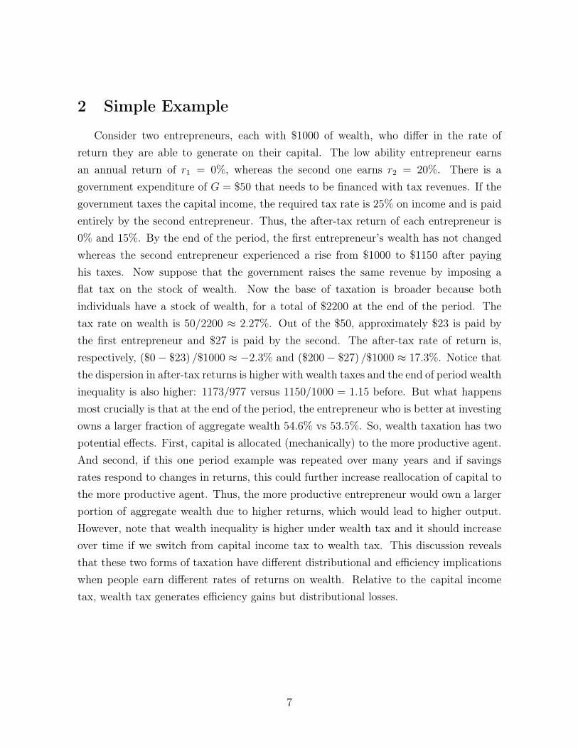
2 Simple Example
Consider two entrepreneurs, each with $1000 of wealth, who differ in the rate ofreturn they are able to generate on their capital. The low ability entrepreneur earnsan annual return of r1 = 0%, whereas the second one earns r2 = 20%. There is agovernment expenditure of G = $50 that needs to be financed with tax revenues. If thegovernment taxes the capital income, the required tax rate is 25% on income and is paidentirely by the second entrepreneur. Thus, the after-tax return of each entrepreneur is0% and 15%. By the end of the period, the first entrepreneur’s wealth has not changedwhereas the second entrepreneur experienced a rise from $1000 to $1150 after payinghis taxes. Now suppose that the government raises the same revenue by imposing aflat tax on the stock of wealth. Now the base of taxation is broader because bothindividuals have a stock of wealth, for a total of $2200 at the end of the period. Thetax rate on wealth is 50/2200 ≈ 2.27%. Out of the $50, approximately $23 is paid bythe first entrepreneur and $27 is paid by the second. The after-tax rate of return is,respectively, ($0− $23) /$1000 ≈ −2.3% and ($200− $27) /$1000 ≈ 17.3%. Notice thatthe dispersion in after-tax returns is higher with wealth taxes and the end of period wealthinequality is also higher: 1173/977 versus 1150/1000 = 1.15 before. But what happensmost crucially is that at the end of the period, the entrepreneur who is better at investingowns a larger fraction of aggregate wealth 54.6% vs 53.5%. So, wealth taxation has twopotential effects. First, capital is allocated (mechanically) to the more productive agent.And second, if this one period example was repeated over many years and if savingsrates respond to changes in returns, this could further increase reallocation of capital tothe more productive agent. Thus, the more productive entrepreneur would own a largerportion of aggregate wealth due to higher returns, which would lead to higher output.However, note that wealth inequality is higher under wealth tax and it should increaseover time if we switch from capital income tax to wealth tax. This discussion revealsthat these two forms of taxation have different distributional and efficiency implicationswhen people earn different rates of returns on wealth. Relative to the capital incometax, wealth tax generates efficiency gains but distributional losses.
7
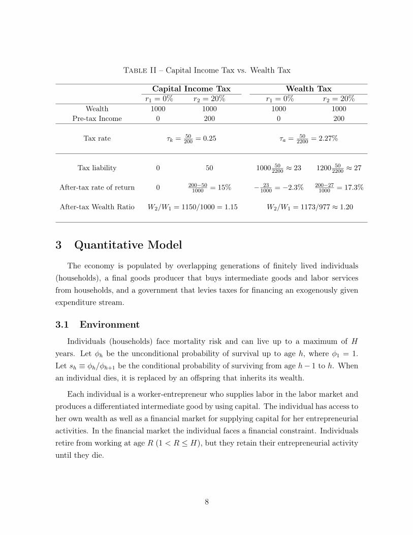
Table II – Capital Income Tax vs. Wealth Tax
Capital Income Tax Wealth Taxr1 = 0% r2 = 20% r1 = 0% r2 = 20%
Wealth 1000 1000 1000 1000Pre-tax Income 0 200 0 200
Tax rate τk = 50200 = 0.25 τa = 50
2200 = 2.27%
Tax liability 0 50 1000 502200 ≈ 23 1200 50
2200 ≈ 27
After-tax rate of return 0 200−501000 = 15% − 23
1000 = −2.3% 200−271000 = 17.3%
After-tax Wealth Ratio W2/W1 = 1150/1000 = 1.15 W2/W1 = 1173/977 ≈ 1.20
3 Quantitative Model
The economy is populated by overlapping generations of finitely lived individuals(households), a final goods producer that buys intermediate goods and labor servicesfrom households, and a government that levies taxes for financing an exogenously givenexpenditure stream.
3.1 Environment
Individuals (households) face mortality risk and can live up to a maximum of Hyears. Let φh be the unconditional probability of survival up to age h, where φ1 = 1.Let sh ≡ φh/φh+1 be the conditional probability of surviving from age h− 1 to h. Whenan individual dies, it is replaced by an offspring that inherits its wealth.
Each individual is a worker-entrepreneur who supplies labor in the labor market andproduces a differentiated intermediate good by using capital. The individual has access toher own wealth as well as a financial market for supplying capital for her entrepreneurialactivities. In the financial market the individual faces a financial constraint. Individualsretire from working at age R (1 < R ≤ H), but they retain their entrepreneurial activityuntil they die.
8
Preferences. Individual preferences are given by:
E0
(H∑h=1
βh−1φhu(ch, `h)
),
where ch is consumption at age h while `h is leisure at age h.1
Labor market productivity. At a given age individuals differ in their labor marketability, yih, which consists of three components
log yih = θi︸︷︷︸permanent
+ κh︸︷︷︸lifecycle
+ eih︸︷︷︸AR(1)
where θi is an individual fixed effect, κh is a life-cycle component that is common to allindividuals and eih follows an AR(1) process during working years (h < R):
eih = ρeei,h−1 + εe,
where εe is an i.i.d. shock with mean zero and variance σ2εe . When an individual dies at
age h, she is replaced by her offspring with h = 1 that inherits her wealth. Individual-specific labor market ability θ is imperfectly inherited from parents:
θchild = ρθθparent + εθ,
where εθ is an i.i.d. shock with mean zero and variance σ2εθ.
Given the wage rate w per efficiency units of labor, the individual’s labor income isgiven by wyihn where n is the hours supplied in the market.
Entrepreneurial process. The key feature of the model is heterogeneity in (average)return to capital, without which capital income taxes and wealth taxes can have identicaleffects.2 Individual i owns the product line i and produces xih units of intermediate goodi according to
xih = zihkih,
1There is no bequest motive. We consider a bequest motive in one of the extensions of the paper.2Notice that wealth and capital income taxes can have different implications even when marginal
returns are equal across individuals, if average returns are different. This will be the case in versionsof our baseline model below. But to see a simpler example with linear returns—so that marginal andaverage returns are equal—suppose that all individuals earn the same average rate of return r on wealth.In this case, consider the budget constraint of a household under two tax systems (capital income tax
9
where zih is the individual i’s entrepreneurial ability and kih is capital. Entrepreneurialability zih has a permanent and a stochastic component. As a result,
zih = f(zpi , zsih)
where zpi captures permanent differences in entrepreneurial ability while zsih capturesvariations over the life-cycle. zsih is governed by the transition matrix Πz while a newborninherits zpi imperfectly from her parent:
log(zpchild) = ρz log(zpparent) + εz,
where εz is an i.i.d. shock with mean zero and variance σ2εz . Due to the imperfect
correlation between the parent’s and child’s ability, some children end up with largeamount of wealth but with low entrepreneurial ability. Similarly, some children withlittle assets at the beginning of their life have high entrepreneurial abilities.
In particular, we assume that zsih ∈ H,L, 0 such that
zih = f(zpi , zsih) =
(zpi )
ω if zsih = H where ω > 1
zpi if zsih = L
0 if zsih = 0
and wealth tax) ignoring other taxes for simplicity:
c+ a′ = [1 + r (1− τk)] a+ wn when capital income is taxed at rate τkc+ a′ = (1 + r) (1− τa) a+ wn when wealth stock is taxed at rate τa,
where a is wealth, r is the interest rate, and wn is the labor income. Suppose the government has tofinance the same amount of expenditures G in both cases. Then,
G = τkr
∫a
aΓ(da) = τa (1 + r)
∫a
aΓ(da),
where Γ(a) is the distribution of agents over wealth. The government budget constraint implies that
τkr = τa (1 + r)⇒ τa =rτk
1 + r
If we insert τa into the after-tax return in the wealth tax we obtain
(1 + r) (1− τa) = (1 + r)
(1− rτk
1 + r
)= 1 + r (1− τk)
Therefore, the budget constraint of the household under two tax systems are the same, so the decisionrules will be the same.
10
with transition matrix
Πz =
1− p1 − p2 p1 p2
0 1− p2 p2
0 0 1
.Finally, individuals whose permanent ability is above the median permanent abil-
ity—i.e., zp > zpmed = 1—start life in state zsih = H while the rest start in state zsih = L.
Financial markets. There are financial market frictions that restrict the extent towhich individuals can borrow to invest in their business. In particular, an individualwith assets a faces a financial constraint
k ≤ ϑ(zih)a,
where ϑ(zih) ∈ [1,∞]. The dependence of ϑ on zih is to allow for the fact that morehighly productive agents could potentially borrow more with the same level of capital.This is a feature that we will have in the baseline calibration and will also consider thecase with ϑ(zih) = ϑ. When ϑ = 1 the financial constraint is extreme since the individualcan only use her own assets in production. When ϑ = ∞ there is no longer a financialconstraint since there is no longer a restriction on the amount that an individual canborrow.
Taxation. Individuals pay a proportional consumption tax, τc, and a proportionalcapital income tax τk. The individual also pays a labor income tax, where for a laborincome of wyihn the after-tax labor income is
(1− τl) (wyihn)ψ ,
where the parameter ψ controls the progressivity of the labor income tax: when ψ = 1
the labor income tax is proportional at the level τl and the progressivity increases withψ.
In our main experiment we will study a revenue-neutral switch to a tax system wherethe government taxes the individual’s wealth stock at the proportional rate τa. We willalso discuss the case where the proportional wealth tax τa is imposed only for wealthabove a certain threshold level, inducing progressivity in the wealth tax.
11
Social security. When an agent retires at age R, she starts receiving social securityincome yR (θ) that depends on her type θ in the following way:
yR (θ, e) = Φ (θ, e)E,
where Φ is the agent’s replacement ratio, a function that depends on the agent’s perma-nent type θ and the last transitory shock to labor productivity, and E which correspondsto the average earnings of the working population in the economy.
Final Goods Producer. The final goods producer behaves competitively and useslabor and intermediate goods in the production of the final good:
Y = QαL1−α,
where Q is the intermediate good aggregator given by
Q =
(∫i
xµi
)1/µ
.
The problem of the final good producer can be written as
maxxi,L
(∫i
xµi
)α/µL1−α −
∫i
pixi − wL,
where pi is the price of the intermediate good i and w is the wage rate. Taking the firstorder conditions, we obtain the following pricing function for intermediate good i
pi (xi) = αxµ−1i Qα−µL1−α,
and the wage ratew = (1− α)QαL−α.
Note that the price of the intermediate good i depends only on the quantity of interme-diate good. Therefore, we can drop i in the price and write the price as only a functionof quantity x
p (x) = αxµ−1Qα−µL1−α.
12
3.2 Individual’s problemFor clarity of notation, in this subsection we suppress the individual subscript i.
Note that the production problem of each agent is static in nature and can be solved inisolation of the other decisions the agent takes. In particular, the agent will maximize theprofits coming from the entrepreneurial activity by choosing an optimal capital demand:
π (a, z) = maxk≤ϑ(z)a
p (zk) zk − (r + δ) k
s.t. p (zk) = P (zk)µ−1 ,
where z = f (zp, zs) and P = αQα−µL1−α. The decision of the individual is then:
k (a, z) = min
(µPzµ
r + δ
) 11−µ
, ϑ(z)a
,
which yields
π (a, z) =
P (zϑ(z)a)µ − (r + δ)ϑ(z)a if k (a, z) = ϑ(z)a
(1− µ)Pzµ(µPzµ
r+δ
) µ1−µ if k (a, z) < ϑ(z)a
.
The household’s after-tax non-labor income, Y (a, z, τk, τa), is given by after-tax prof-its from their firm and interest payments obtained from the financial market:
Y (a, z, τk, τa) = [a+ (π (a, z) + ra) (1− τk)] (1− τa)
The individual’s problem then is given by:
Vh(a,S) = maxc,n,a′
u (c, 1− n) + βsh+1E[Vh+1(a
′,S′) | S
]s.t. (1 + τc) c+ a′ = Y (a, f (zp, zs) , τk, τa) + yW (θ, e)
a′ ≥ 0,
where S = (zp, zs, θ, e) is the vector of exogenous states of an individual and
yW (θ, e) =
(1− τl)(wyhn)ψ if h < R where log yh = θ + κh + e
yR(θ, e) if h ≥ R.
13

We assume that eh = eh−1 for h ≥ R, thus the retirement income is essentially condi-tioned on the earnings shock in period R− 1.
3.3 GovernmentThe government taxes capital income, labor income, and consumption in order to
finance government expenditures G and social security payments. For future referencelet
SSC =∑
h≥R,a,S
yR (θ, e) Γ (h, a,S)
be the total social security payments. Above Γ is the stationary distribution of agentsover all possible states.
To characterize yR (θ, e) we define:
E =wN
IR1
where w is the economy wide wage rate (per efficiency units), IR1 ≤ 1 is the measureof agents in working age, and N is the total number of effective hours worked in theeconomy:
N =∑
h<R,a,S
yh (θ, e)nh (s) Γ (h, a,S)
Note that the summation is taken over efficiency units yh. The replacement ratio isprogressive and satisfies:
Φ (θ, e) =
0.9yR1 (θ,e)
yR1if yR1 (θ,e)
yR1≤ 0.3
0.27 + 0.32(yR1 (θ,e)
yR1− 0.3
)if 0.3 <
yR1 (θ,e)
yR1≤ 2
0.91 + 0.15(yR1 (θ,e)
yR1− 2)
if 2 <yR1 (θ,e)
yR1≤ 4.1
1.1 if 4.1 <yR1 (θ,e)
yR1
where yR1 (θ, e) is the average efficiency units that an agent of type θ gets conditional onhaving a given eR = e.
yR1 (θ, eR) =1
R
∑h<R,a,S
∫yh (θ, e) Γ (h, a,S)
the integral is taken with respect to the stationary distribution of agents by age and is
14

taken over all possible asset holdings, types z, and histories of e such that eR is the onegiven in the left hand side. Finally yR1 is the average of yR1 (θ, e) across θ and e.
3.4 Equilibrium
Let ch(a,S), nh(a,S) and ah+1(a,S) denote the optimal decision rules and Γ (h, a,S)
be the stationary distribution of agents. A competitive equilibrium is given by thefollowing conditions:
1. Consumer’s maximize given p(x), w, r and taxes.
2. The solution to the final goods producer gives pricing function p(x) and wage ratew.
3. Q =(∑
h,a,S (za)µ Γ (h, a,S))1/µ
and L =∑
h,a,S yhnh(a,S)Γ (h, a,S), where log yh =
θ + κh + e.
4. The government budget balances. We will compare the following two alternatives:
(a) Taxing capital and labor income, in which case the government’s budget be-comes
G+ SSC = τk∑h,a,S
(π (a, z) + ra) Γ (h, a,S)
+ τL∑h,a,S
(wyhnh(a,S)) Γ (h, a,S)
+ τc∑h,a,S
ch(a,S)Γ (h, a,S)
whereSSC =
∑h≥R,a,S
yR (θ, e) Γ (h, a,S) .
(b) Taxing wealth stock and labor income, in which case the government’s budget
15

becomes
G+ SSC = τa∑h,a,S
((1 + r) a+ π (a, z)) Γ (h, a,S)
+ τL∑h,a,S
(wyhnh (a,S)) Γ (h, a,S)
+ τc∑h,a,S
ch (a,S) Γ (h, a,S)
5. The bond market clears:
0 =∑h,a,S
(a− k (a, z)) Γ (h, a,S)
4 Quantitative Analysis: Tax Reform
4.1 Model Parameterization
The benchmark model is calibrated to US data. The model period is one year.
Government Policy. The benchmark economy has a proportional capital income taxτk, a proportional labor earnings tax determined by τl, and a proportional consumptiontax τc. Using the results in McDaniel (2007), we calibrate a capital income tax τk of25%, a labor income tax of 22.4%, and a consumption tax of 7.5%.
Demographics. Individuals enter the economy at age 20 and can live up to 80 years(so the maximum real life age is 100). They retire at age R = 46, which is 66 years old.The conditional survival probabilities from age h to h+ 1 are taken from Bell and Miller(2002) for the US data.
Preferences. Individuals value consumption c and leisure `. The utility function takesthe following form
u(c, `) =(cγ`1−γ)1−σ
1− σ.
We calibrate β = 0.9475 to generate a wealth-to-output ratio of 3 in the stationaryequilibrium. The leisure parameter γ = 0.46 is calibrated to match an average hours ofwork of 0.4 for the working age population, i.e. ages 25 to 60, in equilibrium.
16
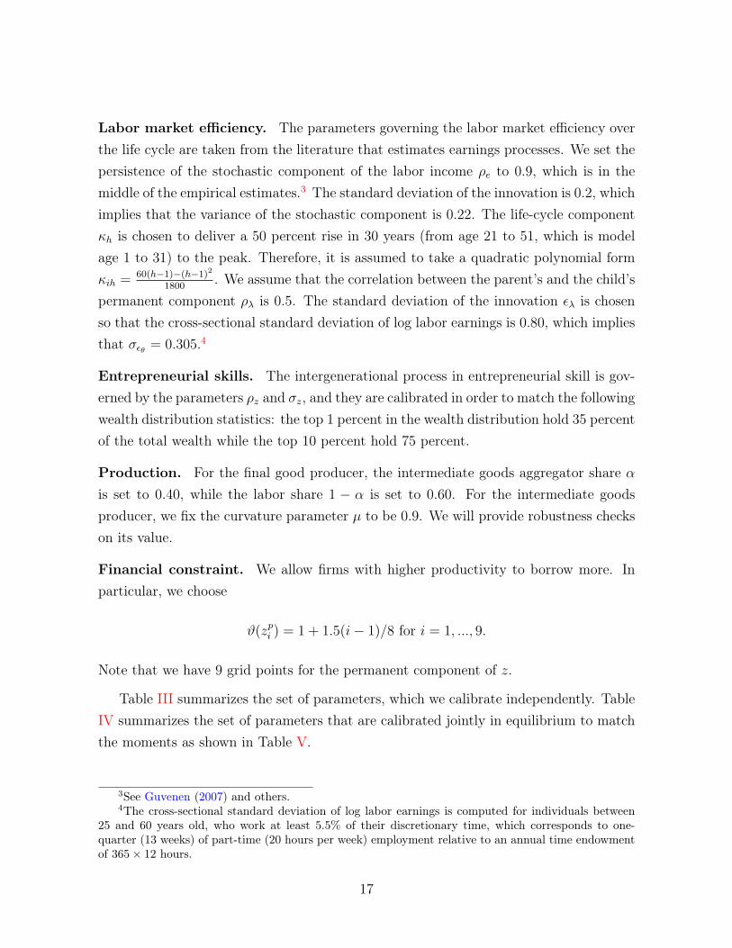
Labor market efficiency. The parameters governing the labor market efficiency overthe life cycle are taken from the literature that estimates earnings processes. We set thepersistence of the stochastic component of the labor income ρe to 0.9, which is in themiddle of the empirical estimates.3 The standard deviation of the innovation is 0.2, whichimplies that the variance of the stochastic component is 0.22. The life-cycle componentκh is chosen to deliver a 50 percent rise in 30 years (from age 21 to 51, which is modelage 1 to 31) to the peak. Therefore, it is assumed to take a quadratic polynomial formκih = 60(h−1)−(h−1)2
1800. We assume that the correlation between the parent’s and the child’s
permanent component ρλ is 0.5. The standard deviation of the innovation ελ is chosenso that the cross-sectional standard deviation of log labor earnings is 0.80, which impliesthat σεθ = 0.305.4
Entrepreneurial skills. The intergenerational process in entrepreneurial skill is gov-erned by the parameters ρz and σz, and they are calibrated in order to match the followingwealth distribution statistics: the top 1 percent in the wealth distribution hold 35 percentof the total wealth while the top 10 percent hold 75 percent.
Production. For the final good producer, the intermediate goods aggregator share αis set to 0.40, while the labor share 1 − α is set to 0.60. For the intermediate goodsproducer, we fix the curvature parameter µ to be 0.9. We will provide robustness checkson its value.
Financial constraint. We allow firms with higher productivity to borrow more. Inparticular, we choose
ϑ(zpi ) = 1 + 1.5(i− 1)/8 for i = 1, ..., 9.
Note that we have 9 grid points for the permanent component of z.
Table III summarizes the set of parameters, which we calibrate independently. TableIV summarizes the set of parameters that are calibrated jointly in equilibrium to matchthe moments as shown in Table V.
3See Guvenen (2007) and others.4The cross-sectional standard deviation of log labor earnings is computed for individuals between
25 and 60 years old, who work at least 5.5% of their discretionary time, which corresponds to one-quarter (13 weeks) of part-time (20 hours per week) employment relative to an annual time endowmentof 365× 12 hours.
17
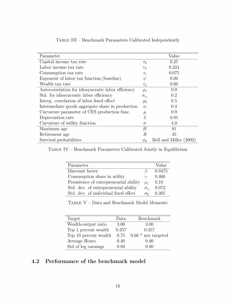
Table III – Benchmark Parameters Calibrated Independently
Parameter ValueCapital income tax rate τk 0.25Labor income tax rate τL 0.224Consumption tax rate τc 0.075Exponent of labor tax function (baseline) ψ 0.00Wealth tax rate τa 0.00Autocorrelation for idiosyncratic labor efficiency ρe 0.9Std. for idiosyncratic labor efficiency σεe 0.2Interg. correlation of labor fixed effect ρθ 0.5Intermediate goods aggregate share in production α 0.4Curvature parameter of CES production func. µ 0.9Depreciation rate δ 0.05Curvature of utility function σ 4.0Maximum age H 81Retirement age R 45Survival probabilities φh Bell and Miller (2002)
Table IV – Benchmark Parameters Calibrated Jointly in Equilibrium
Parameter ValueDiscount factor β 0.9475Consumption share in utility γ 0.460Persistence of entrepreneurial ability ρz 0.10Std. dev. of entrepreneurial ability σεz 0.072Std. dev. of individual fixed effect σθ 0.305
Table V – Data and Benchmark Model Moments
Target Data BenchmarkWealth-output ratio 3.00 3.00Top 1 percent wealth 0.357 0.357Top 10 percent wealth 0.75 0.66 * not targetedAverage Hours 0.40 0.40Std of log earnings 0.80 0.80
4.2 Performance of the benchmark model
18
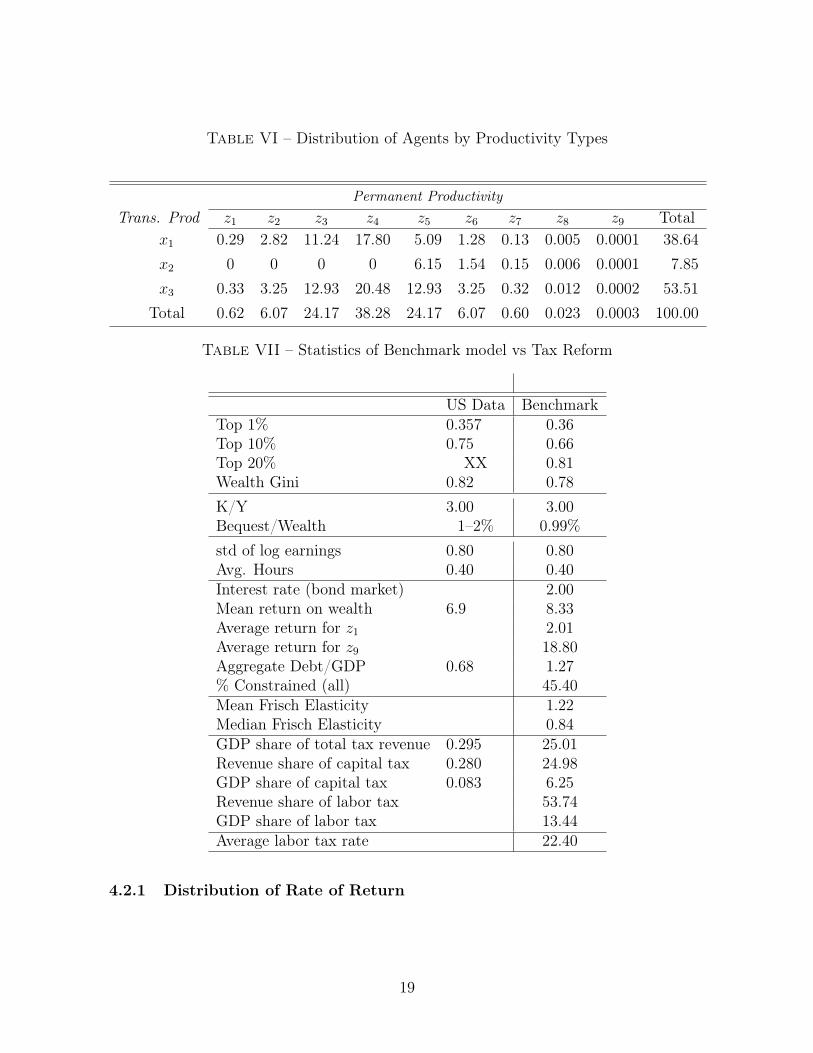
Table VI – Distribution of Agents by Productivity Types
Permanent ProductivityTrans. Prod z1 z2 z3 z4 z5 z6 z7 z8 z9 Total
x1 0.29 2.82 11.24 17.80 5.09 1.28 0.13 0.005 0.0001 38.64x2 0 0 0 0 6.15 1.54 0.15 0.006 0.0001 7.85x3 0.33 3.25 12.93 20.48 12.93 3.25 0.32 0.012 0.0002 53.51
Total 0.62 6.07 24.17 38.28 24.17 6.07 0.60 0.023 0.0003 100.00
Table VII – Statistics of Benchmark model vs Tax Reform
US Data BenchmarkTop 1% 0.357 0.36Top 10% 0.75 0.66Top 20% XX 0.81Wealth Gini 0.82 0.78K/Y 3.00 3.00Bequest/Wealth 1–2% 0.99%std of log earnings 0.80 0.80Avg. Hours 0.40 0.40Interest rate (bond market) 2.00Mean return on wealth 6.9 8.33Average return for z1 2.01Average return for z9 18.80Aggregate Debt/GDP 0.68 1.27% Constrained (all) 45.40Mean Frisch Elasticity 1.22Median Frisch Elasticity 0.84GDP share of total tax revenue 0.295 25.01Revenue share of capital tax 0.280 24.98GDP share of capital tax 0.083 6.25Revenue share of labor tax 53.74GDP share of labor tax 13.44Average labor tax rate 22.40
4.2.1 Distribution of Rate of Return
19
Table VIII – Percentiles of Rate of Return Distribution, Benchmark Model
p10 p25 p50 p60 p75 p80 p90 p95 p99.9Unweighted (%) 2 2 2 6.6 12 13.3 17.3 22.4 76.6(Wealth) weighted (%) 2 2 5.3 8.8 11.7 13.1 20.4 26.4 50.2
20 30 40 50 60 70 80 90 100
Age
0
50
100
150
200
250
300
Re
turn
(%
)
Mean Return
Meanz1z2z3z4z5z6z7z8z9
(a) Unweighted Returns
20 30 40 50 60 70 80 90 100
Age
0
20
40
60
80
100
120
140
160
180
We
igh
ted
Re
turn
(%
)
Weighted Return by Prod. Levels
Meanz1z2z3z4z5z6z7z8z9
(b) Weighted Returns
Figure 1 – Deciles of the Rate of Return Distribution Over Life Cycle, Benchmark
Standard Deviation of Return by Age
Unweighted return - Assets The return for each age group is computed as:
r =1
T
∑t
Pr (at, z, xt) +Ratat
where:
Pr (at, z, xt) = p (ztkt)µ − (R + δ) kt kt = min θ (z) at , k
? (z, xt)
Weighted return - Assets The return for each age group is computed as:
r =
∑t Pr (at, z, xt) +Rat∑
t at
20

Table IX – Unweighed Returns of Assets by Age Group - Benchmark Model
Age 20 21-25 26-30 31-35 36-40 41-45 46-50 51-55 56-60 61-65 66-70 AllStd Dev 77.9 10.0 8.3 6.0 7.9 5.8 5.2 4.8 4.5 4.6 4.4 9.1Mean 79.9 16.2 12.0 7.9 9.7 6.7 5.8 5.1 4.7 4.5 4.2 7.0p99.9 690.6 71.5 58.6 40.1 45.3 33.0 30.0 28.4 25.7 25.9 22.4 76.6p99 416.6 47.2 38.4 27.5 35.1 24.5 21.1 19.0 17.8 19.8 18.9 42.7p95 219.0 31.9 25.9 18.0 23.7 17.2 15.5 14.4 13.9 14.4 14.1 22.3p90 148.3 28.9 22.9 15.4 19.8 14.5 13.3 12.5 12.1 12.1 11.9 17.3p75 96.6 20.0 16.1 11.4 15.3 11.3 10.0 8.6 6.7 5.0 2.0 12.0p50 63.7 15.3 11.5 7.2 8.0 3.5 2.0 2.0 2.0 2.0 2.0 2.0p25 32.8 9.5 5.3 1.6 2.4 2.0 2.0 2.0 2.0 2.0 2.0 2.0p10 16.9 5.3 2.0 1.6 2.4 2.0 2.0 2.0 2.0 2.0 2.0 2.0p1 5.8 2.0 2.0 1.6 2.4 2.0 2.0 2.0 2.0 2.0 2.0 2.0
where:
Pr (at, z, xt) = p (ztkt)µ − (R + δ) kt kt = min θ (z) at , k
? (z, xt)
Table X – Weighed Returns of Assets by Age Group - Benchmark Model
Age 20 21-25 26-30 31-35 36-40 41-45 46-50 51-55 56-60 61-65 66-70 AllStd Dev 8.1 9.6 8.2 7.4 6.5 5.8 5.2 4.8 4.5 4.4 4.4 8.5Mean 7.4 15.5 11.9 9.8 8.0 6.7 5.8 5.1 4.6 4.4 4.2 8.4p99.9 76.6 68.1 57.5 49.2 38.6 32.5 29.6 28.1 25.8 23.5 22.3 27.9p99 39.3 45.5 38.1 34.2 28.8 23.9 20.7 18.8 17.7 18.1 18.8 26.6p95 19.2 30.7 25.7 22.4 19.5 17.1 15.4 14.3 13.8 14.1 14.1 22.0p90 15.2 27.8 22.6 19.1 16.3 14.4 13.3 12.5 12.0 12.0 11.9 17.0p75 10.1 19.3 16.0 14.1 12.7 11.2 10.0 8.6 6.7 5.0 2.0 11.1p50 4.6 14.4 11.3 8.9 6.6 3.4 2.0 2.0 2.0 2.0 2.0 4.6p25 2.2 9.0 5.2 2.0 2.0 2.0 2.0 2.0 2.0 2.0 2.0 2.0p10 2.0 4.8 2.0 2.0 2.0 2.0 2.0 2.0 2.0 2.0 2.0 2.0p1 2.0 2.0 2.0 2.0 2.0 2.0 2.0 2.0 2.0 2.0 2.0 2.0
Unweighted return - Capital The return for each age group is computed as:
r =1∑
t 1kt>0
∑t
Pr (at, z, xt) +Ratkt
1kt>0
where:
Pr (at, z, xt) = p (ztkt)µ − (R + δ) kt kt = min θ (z) at , k
? (z, xt)
21
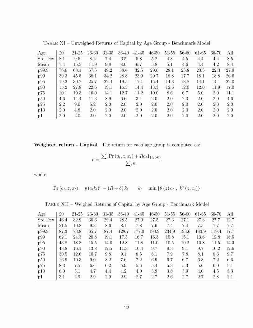
Table XI – Unweighed Returns of Capital by Age Group - Benchmark Model
Age 20 21-25 26-30 31-35 36-40 41-45 46-50 51-55 56-60 61-65 66-70 AllStd Dev 8.1 9.6 8.2 7.4 6.5 5.8 5.2 4.8 4.5 4.4 4.4 8.5Mean 7.4 15.5 11.9 9.8 8.0 6.7 5.8 5.1 4.6 4.4 4.2 8.4p99.9 76.6 68.1 57.5 49.2 38.6 32.5 29.6 28.1 25.8 23.5 22.3 27.9p99 39.3 45.5 38.1 34.2 28.8 23.9 20.7 18.8 17.7 18.1 18.8 26.6p95 19.2 30.7 25.7 22.4 19.5 17.1 15.4 14.3 13.8 14.1 14.1 22.0p90 15.2 27.8 22.6 19.1 16.3 14.4 13.3 12.5 12.0 12.0 11.9 17.0p75 10.1 19.3 16.0 14.1 12.7 11.2 10.0 8.6 6.7 5.0 2.0 11.1p50 4.6 14.4 11.3 8.9 6.6 3.4 2.0 2.0 2.0 2.0 2.0 4.6p25 2.2 9.0 5.2 2.0 2.0 2.0 2.0 2.0 2.0 2.0 2.0 2.0p10 2.0 4.8 2.0 2.0 2.0 2.0 2.0 2.0 2.0 2.0 2.0 2.0p1 2.0 2.0 2.0 2.0 2.0 2.0 2.0 2.0 2.0 2.0 2.0 2.0
Weighted return - Capital The return for each age group is computed as:
r =
∑t Pr (at, z, xt) +Rat1kt>0∑
t kt
where:
Pr (at, z, xt) = p (ztkt)µ − (R + δ) kt kt = min θ (z) at , k
? (z, xt)
Table XII – Weighed Returns of Capital by Age Group - Benchmark Model
Age 20 21-25 26-30 31-35 36-40 41-45 46-50 51-55 56-60 61-65 66-70 AllStd Dev 46.4 32.9 30.6 29.4 28.5 27.9 27.5 27.3 27.1 27.3 27.7 12.7Mean 21.5 10.8 9.3 8.6 8.1 7.8 7.6 7.4 7.4 7.5 7.7 7.7p99.9 87.3 73.8 65.7 87.4 128.7 177.0 190.9 234.9 193.6 183.9 119.4 17.7p99 62.1 24.3 20.8 19.1 17.5 16.7 16.3 15.8 15.1 13.6 12.8 16.5p95 43.8 18.8 15.5 14.0 12.8 11.8 11.0 10.5 10.2 10.8 11.5 14.3p90 43.8 16.1 13.8 12.5 11.3 10.4 9.7 9.3 9.1 9.7 10.2 12.6p75 30.5 12.6 10.7 9.8 9.1 8.5 8.1 7.9 7.8 8.1 8.6 9.7p50 16.9 10.3 9.0 8.2 7.6 7.2 6.9 6.7 6.7 6.8 7.2 6.6p25 8.3 7.5 6.6 6.2 5.9 5.6 5.4 5.3 5.3 5.6 6.0 5.1p10 6.0 5.1 4.7 4.4 4.2 4.0 3.9 3.8 3.9 4.0 4.5 3.3p1 3.1 2.9 2.9 2.9 2.9 2.7 2.7 2.6 2.7 2.7 2.8 2.1
22

Table XIII – Percentiles of Wealth Distribution
p10 p25 p50 p60 p75 p80 p90 p95 p99.9Assets 7.5 10713.5 66432.6 109603.9 221621.9 282558.9 503725.9 788464.5 12127732.9
4.2.2 Wealth distribution, the Pareto tail, and assets deciles.
Figure 2 – Asset Deciles by Age
20 30 40 50 60 70 80 90 100
Age
0
1
2
3
4
5
6
7
8
We
alth (
$)
×105 Wealth Decile by age
d1d2d3d4d5d6d7d8d9
There are two formats we have used for the Pareto tail graph I’m attaching themboth.
Table XIV – Pareto Coefficient for distribution of wealth above 1 million dollars
BaselineTail Coeff. W > 1e6 1.46
23
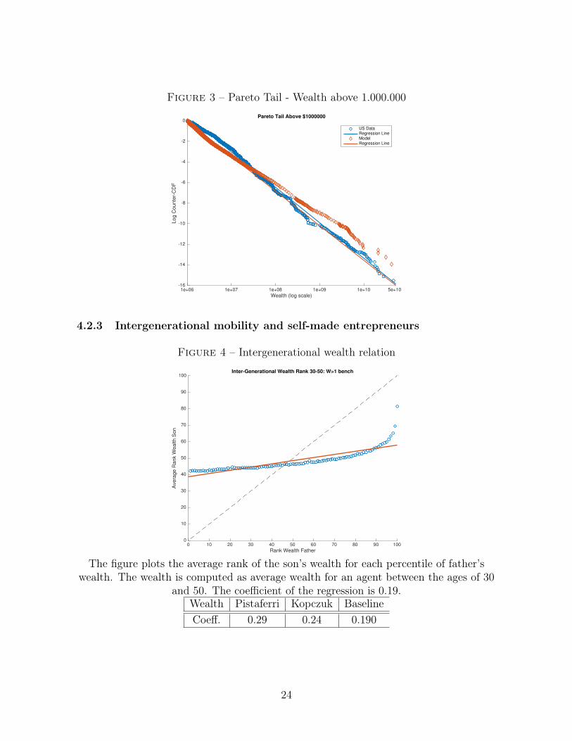
Figure 3 – Pareto Tail - Wealth above 1.000.000
1e+06 1e+07 1e+08 1e+09 1e+10 5e+10
Wealth (log scale)
-16
-14
-12
-10
-8
-6
-4
-2
0
Lo
g C
ounte
r-C
DF
Pareto Tail Above $1000000
US DataRegression LineModelRegression Line
4.2.3 Intergenerational mobility and self-made entrepreneurs
Figure 4 – Intergenerational wealth relation
0 10 20 30 40 50 60 70 80 90 100
Rank Wealth Father
0
10
20
30
40
50
60
70
80
90
100
Ave
rag
e R
ank W
ealth
Son
Inter-Generational Wealth Rank 30-50: W>1 bench
The figure plots the average rank of the son’s wealth for each percentile of father’swealth. The wealth is computed as average wealth for an agent between the ages of 30
and 50. The coefficient of the regression is 0.19.Wealth Pistaferri Kopczuk BaselineCoeff. 0.29 0.24 0.190
24

Figure 5 – Intergenerational return relation
0 10 20 30 40 50 60 70 80 90 100
Rank Return Father
0
10
20
30
40
50
60
70
80
90
100
Avera
ge R
ank R
etu
rn S
on
Inter-Generational Return Rank 30-50: W>1 bench
The figure plots the average rank of the son’s return for each percentile of father’sreturn. The return is computed as average return for an agent between the ages of 30
and 50. The coefficient of the regression is –0.002.Pistaferri Book Value
Coeff. –0.002
4.2.4 Top 80 Agents
Table XV – Statistics on the Top 80 agents of the simulation
WNB < 1, 000, 000 38.8%Initial percentile < 90 38.8%WNB/WT > 100 50.0%WNB/WT > 1, 000 47.5%Constrained Initial 55.0%Constrained Final 27.5%Mean Leverage Initial 32.1%Mean Leverage Final –26.4%
Leverage is measured as the debt-to-equity ratio.
25
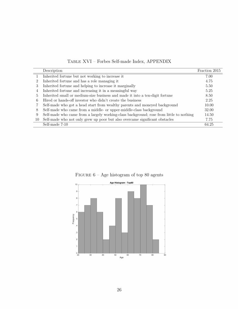
Table XVI – Forbes Self-made Index, APPENDIX
Description Fraction 20151 Inherited fortune but not working to increase it 7.002 Inherited fortune and has a role managing it 4.753 Inherited fortune and helping to increase it marginally 5.504 Inherited fortune and increasing it in a meaningful way 5.255 Inherited small or medium-size business and made it into a ten-digit fortune 8.506 Hired or hands-off investor who didn’t create the business 2.257 Self-made who got a head start from wealthy parents and moneyed background 10.008 Self-made who came from a middle- or upper-middle-class background 32.009 Self-made who came from a largely working-class background; rose from little to nothing 14.5010 Self-made who not only grew up poor but also overcame significant obstacles 7.75
Self-made 7-10 64.25
Figure 6 – Age histogram of top 80 agents
20 30 40 50 60 70 80 90
Age
0
1
2
3
4
5
6
7
8
9
10
Fre
qu
en
cy
Age Histogram - Top80
26
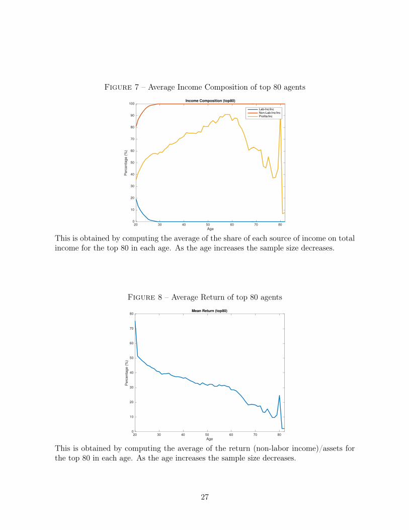
Figure 7 – Average Income Composition of top 80 agents
20 30 40 50 60 70 80
Age
0
10
20
30
40
50
60
70
80
90
100
Perc
en
tage
(%
)
Income Composition (top80)
Lab-Inc/IncNon-Lab-Inc/IncProfits/Inc
This is obtained by computing the average of the share of each source of income on totalincome for the top 80 in each age. As the age increases the sample size decreases.
Figure 8 – Average Return of top 80 agents
20 30 40 50 60 70 80
Age
0
10
20
30
40
50
60
70
80
Perc
enta
ge (
%)
Mean Return (top80)
This is obtained by computing the average of the return (non-labor income)/assets forthe top 80 in each age. As the age increases the sample size decreases.
27

4.2.5 Constrained producers and leverage.
Table XVII – Optimal capital level and percentage of constrained agents by produc-tivity
Book ValueHigh Shock Low ShockK Const. K Const.
z1 3990 32.6z2 116742 70.2z3 3029913 99.5z4 78638108 100.0z5 2040966891 100.0 150825105 100.0z6 52971084173 100.0 289277209 100.0z7 1374807093290 100.0 554823437 99.9z8 35681628444367 100.0 1064131696 97.5z9 926078003710803 100.0 2040966891 91.3
Figure 9 – Constrained Firms by productivity and age
20 30 40 50 60 70 80 90 100
Age
0
10
20
30
40
50
60
70
80
90
100
Share
of C
on
st.
Firm
s (
%)
Share of Const. Firms
Meanz1z2z3z4z5z6z7z8z9
28

Figure 10 – Constrained Firms by wealth decile and age
20 30 40 50 60 70 80 90 100
Age
0
10
20
30
40
50
60
70
80
90
100
110
% o
f C
on
st. F
irm
s
% Const. Firms by Wealth Decile
d1d2d3d4d5d6d7d8d9d10
4.2.6 Leverage (Leverage is measured as the debt-to-equity ratio. )
Table XVIII – Percentiles of leverage distribution
p10 p25 p50 p60 p75 p80 p90 p95 p99.9Leverage 0 0 0 37.5 56.3 56.3 75 75 112.5
Leverage is measured as the debt-to-equity ratio.
29
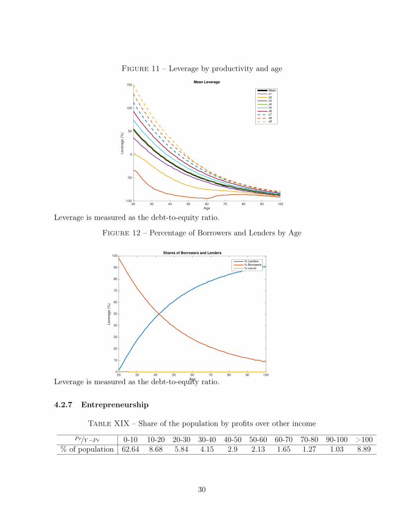
Figure 11 – Leverage by productivity and age
20 30 40 50 60 70 80 90 100
Age
-100
-50
0
50
100
150
Le
vera
ge (
%)
Mean Leverage
Meanz1z2z3z4z5z6z7z8z9
Leverage is measured as the debt-to-equity ratio.
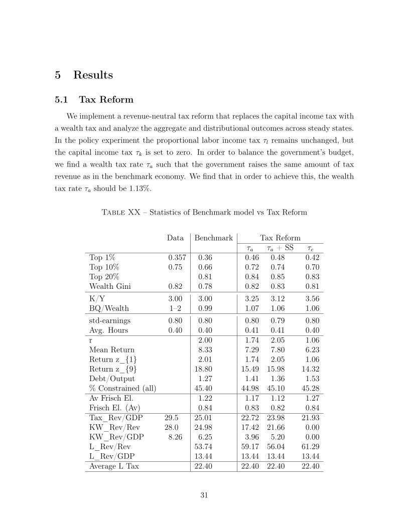
Figure 12 – Percentage of Borrowers and Lenders by Age
20 30 40 50 60 70 80 90 100
Age
0
10
20
30
40
50
60
70
80
90
100
Levera
ge (
%)
Shares of Borrowers and Lenders
% Lenders% Borrowers% Lev=0
Leverage is measured as the debt-to-equity ratio.
4.2.7 Entrepreneurship
Table XIX – Share of the population by profits over other income
Pr/Y−Pr 0-10 10-20 20-30 30-40 40-50 50-60 60-70 70-80 90-100 >100% of population 62.64 8.68 5.84 4.15 2.9 2.13 1.65 1.27 1.03 8.89
30
5 Results
5.1 Tax Reform
We implement a revenue-neutral tax reform that replaces the capital income tax witha wealth tax and analyze the aggregate and distributional outcomes across steady states.In the policy experiment the proportional labor income tax τl remains unchanged, butthe capital income tax τk is set to zero. In order to balance the government’s budget,we find a wealth tax rate τa such that the government raises the same amount of taxrevenue as in the benchmark economy. We find that in order to achieve this, the wealthtax rate τa should be 1.13%.
Table XX – Statistics of Benchmark model vs Tax Reform
Data Benchmark Tax Reformτa τa + SS τc
Top 1% 0.357 0.36 0.46 0.48 0.42Top 10% 0.75 0.66 0.72 0.74 0.70Top 20% 0.81 0.84 0.85 0.83Wealth Gini 0.82 0.78 0.82 0.83 0.81K/Y 3.00 3.00 3.25 3.12 3.56BQ/Wealth 1–2 0.99 1.07 1.06 1.06std-earnings 0.80 0.80 0.80 0.79 0.80Avg. Hours 0.40 0.40 0.41 0.41 0.40r 2.00 1.74 2.05 1.06Mean Return 8.33 7.29 7.80 6.23Return z_1 2.01 1.74 2.05 1.06Return z_9 18.80 15.49 15.98 14.32Debt/Output 1.27 1.41 1.36 1.53% Constrained (all) 45.40 44.98 45.10 45.28Av Frisch El. 1.22 1.17 1.12 1.27Frisch El. (Av) 0.84 0.83 0.82 0.84Tax_Rev/GDP 29.5 25.01 22.72 23.98 21.93KW_Rev/Rev 28.0 24.98 17.42 21.66 0.00KW_Rev/GDP 8.26 6.25 3.96 5.20 0.00L_Rev/Rev 53.74 59.17 56.04 61.29L_Rev/GDP 13.44 13.44 13.44 13.44Average L Tax 22.40 22.40 22.40 22.40
31
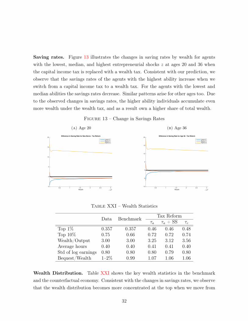
Saving rates. Figure 13 illustrates the changes in saving rates by wealth for agentswith the lowest, median, and highest entrepreneurial shocks z at ages 20 and 36 whenthe capital income tax is replaced with a wealth tax. Consistent with our prediction, weobserve that the savings rates of the agents with the highest ability increase when weswitch from a capital income tax to a wealth tax. For the agents with the lowest andmedian abilities the savings rates decrease. Similar patterns arise for other ages too. Dueto the observed changes in savings rates, the higher ability individuals accumulate evenmore wealth under the wealth tax, and as a result own a higher share of total wealth.
Figure 13 – Change in Savings Rates
(a) Age 20
0.5 1 1.5 2 2.5 3
Wealth×10
6
-5
0
5
10
15
20Difference in Saving Rate for New Borns - Tax Reform
Lowest ZMedian ZHighest Z
(b) Age 36
0.5 1 1.5 2 2.5 3
Wealth×10
6
-10
-5
0
5
10
15
20Difference in Saving Rate for Age 36 - Tax Reform
Lowest ZMedian ZHighest Z
Table XXI – Wealth Statistics
Data Benchmark Tax Reformτa τa + SS τc
Top 1% 0.357 0.357 0.46 0.46 0.48Top 10% 0.75 0.66 0.72 0.72 0.74Wealth/Output 3.00 3.00 3.25 3.12 3.56Average hours 0.40 0.40 0.41 0.41 0.40Std of log earnings 0.80 0.80 0.80 0.79 0.80Bequest/Wealth 1–2% 0.99 1.07 1.06 1.06
Wealth Distribution. Table XXI shows the key wealth statistics in the benchmarkand the counterfactual economy. Consistent with the changes in savings rates, we observethat the wealth distribution becomes more concentrated at the top when we move from
32
an economy with a capital income tax to a one with a wealth tax. The fraction of wealthheld by the households in the top 1 percent increases from 36 percent to 46 percent,while the fraction of wealth held by the households in the top 10 percent increases from66 percent to 72 percent. The wealth-to-output ratio also increases from 3 to 3.25.
Aggregate Variables. Table XXII lists the aggregate variables in the two economies.Since wealth is more concentrated in the hands of more productive agents under wealthtax, the aggregate intermediate goods aggregator increases by 24.8 percent. Therefore,the aggregate output increases by 10.1 percent.
Table XXII – Equilibrium Variables
BenchmarkTax Reform
τa τa + SS τcLevel % Change Level % Change Level % Change
Capital income tax rate τk 25% 0 - - 0 -Wealth tax rate rate τa 0 1.13% - 1.54% - 0 -Consumption tax rate τc 7.5% 7.5% - 7.5% - 12.16% -Aggregate Capital k 3.50 4.18 19.4 3.93 12.3 4.74 35.3Intermediate goods Q 3.51 4.38 24.8 4.15 18.4 4.87 38.8Wage w 1.25 1.36 8.7 1.33 6.4 1.42 14.0Output Y 1.17 1.28 10.1 1.26 7.9 1.33 14.1Labor L 0.56 0.57 1.3 0.57 1.4 0.56 0.1Consumption C 0.83 0.91 10.0 0.90 8.4 0.93 12.2TFPQ 1.001 1.047 4.60 1.06 5.51 1.027 2.60TFP?Q/TFPQ 1.582 1.514 - 1.50 - 0.120 -
Welfare. Given our utility function specification, the welfare consequences of switchingfrom the benchmark economy to a counterfactual economy with a wealth tax for ahousehold in state S with age h and wealth a is given by
CEh(a,S) = 100×
[(Vh(a,S; τ policy)
Vh(a,S; τ bench)
)1/γ(1−σ)
− 1
].
This measure specifically gives what fraction of consumption a household is willing topay in order to move from the steady state of the economy with a capital income tax tothe steady state of the economy with a wealth tax.
33
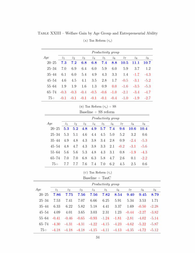
Table XXIII – Welfare Gain by Age Group and Entrepreneurial Ability
(a) Tax Reform (τa)
Productivity groupAge z1 z2 z3 z4 z5 z6 z7 z8 z9
20–25 7.3 7.2 6.8 6.8 7.4 8.8 10.5 11.1 10.725–34 7.0 6.9 6.4 6.0 5.9 6.0 5.9 3.7 1.235–44 6.1 6.0 5.4 4.9 4.3 3.3 1.4 -1.7 -4.345–54 4.6 4.5 4.1 3.5 2.8 1.7 -0.5 -3.1 -5.255–64 1.9 1.9 1.6 1.3 0.9 0.0 -1.6 -3.5 -5.365–74 -0.3 -0.3 -0.4 -0.5 -0.6 -1.0 -2.1 -3.4 -4.775+ -0.1 -0.1 -0.1 -0.1 -0.1 -0.4 -1.0 -1.9 -2.7
(b) Tax Reform (τa) + SS
Baseline + SS reform
Productivity groupAge z1 z2 z3 z4 z5 z6 z7 z8 z9
20–25 5.3 5.2 4.8 4.9 5.7 7.4 9.6 10.6 10.425–34 5.3 5.1 4.6 4.4 4.5 5.0 5.2 3.2 0.635–44 4.9 4.8 4.3 3.8 3.4 2.8 0.9 -2.4 -5.345–54 4.8 4.7 4.3 3.8 3.3 2.1 -0.2 -3.1 -5.655–64 5.6 5.6 5.3 4.8 4.3 3.1 0.8 -1.9 -4.365–74 7.0 7.0 6.8 6.3 5.8 4.7 2.6 0.1 -2.275+ 7.7 7.7 7.6 7.4 7.0 6.2 4.5 2.5 0.6
(c) Tax Reform (τc)
Baseline + TauC
Productivity groupAge z1 z2 z3 z4 z5 z6 z7 z8 z9
20–25 7.86 7.75 7.56 7.56 7.82 8.54 9.40 9.45 8.7925–34 7.53 7.41 7.07 6.66 6.25 5.91 5.34 3.53 1.7135–44 6.33 6.22 5.82 5.18 4.41 3.37 1.69 -0.50 -2.2845–54 4.09 4.01 3.65 3.03 2.31 1.23 -0.44 -2.27 -3.8255–64 -0.41 -0.46 -0.65 -0.93 -1.24 -1.81 -2.81 -4.02 -5.1465–74 -4.30 -4.31 -4.31 -4.22 -4.15 -4.23 -4.62 -5.22 -5.8775+ -4.18 -4.18 -4.18 -4.15 -4.11 -4.13 -4.35 -4.72 -5.12
34
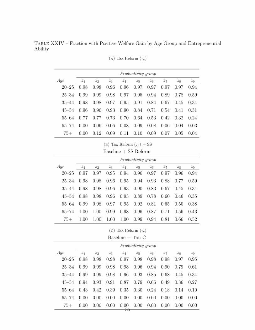
Table XXIV – Fraction with Positive Welfare Gain by Age Group and EntrepreneurialAbility
(a) Tax Reform (τa)
Productivity groupAge z1 z2 z3 z4 z5 z6 z7 z8 z9
20–25 0.98 0.98 0.96 0.96 0.97 0.97 0.97 0.97 0.9425–34 0.99 0.99 0.98 0.97 0.95 0.94 0.89 0.78 0.5935–44 0.98 0.98 0.97 0.95 0.91 0.84 0.67 0.45 0.3445–54 0.96 0.96 0.93 0.90 0.84 0.71 0.54 0.41 0.3155–64 0.77 0.77 0.73 0.70 0.64 0.53 0.42 0.32 0.2465–74 0.00 0.06 0.06 0.08 0.09 0.08 0.06 0.04 0.0375+ 0.00 0.12 0.09 0.11 0.10 0.09 0.07 0.05 0.04
(b) Tax Reform (τa) + SS
Baseline + SS Reform
Productivity groupAge z1 z2 z3 z4 z5 z6 z7 z8 z9
20–25 0.97 0.97 0.95 0.94 0.96 0.97 0.97 0.96 0.9425–34 0.98 0.98 0.96 0.95 0.94 0.93 0.88 0.77 0.5935–44 0.98 0.98 0.96 0.93 0.90 0.83 0.67 0.45 0.3445–54 0.98 0.98 0.96 0.93 0.89 0.78 0.60 0.46 0.3555–64 0.99 0.98 0.97 0.95 0.92 0.81 0.65 0.50 0.3865–74 1.00 1.00 0.99 0.98 0.96 0.87 0.71 0.56 0.4375+ 1.00 1.00 1.00 1.00 0.99 0.94 0.81 0.66 0.52
(c) Tax Reform (τc)
Baseline + Tau C
Productivity groupAge z1 z2 z3 z4 z5 z6 z7 z8 z9
20–25 0.98 0.98 0.98 0.97 0.98 0.98 0.98 0.97 0.9525–34 0.99 0.99 0.98 0.98 0.96 0.94 0.90 0.79 0.6135–44 0.99 0.99 0.98 0.96 0.93 0.85 0.68 0.45 0.3445–54 0.94 0.93 0.91 0.87 0.79 0.66 0.49 0.36 0.2755–64 0.43 0.42 0.39 0.35 0.30 0.24 0.18 0.14 0.1065–74 0.00 0.00 0.00 0.00 0.00 0.00 0.00 0.00 0.0075+ 0.00 0.00 0.00 0.00 0.00 0.00 0.00 0.00 0.00
35
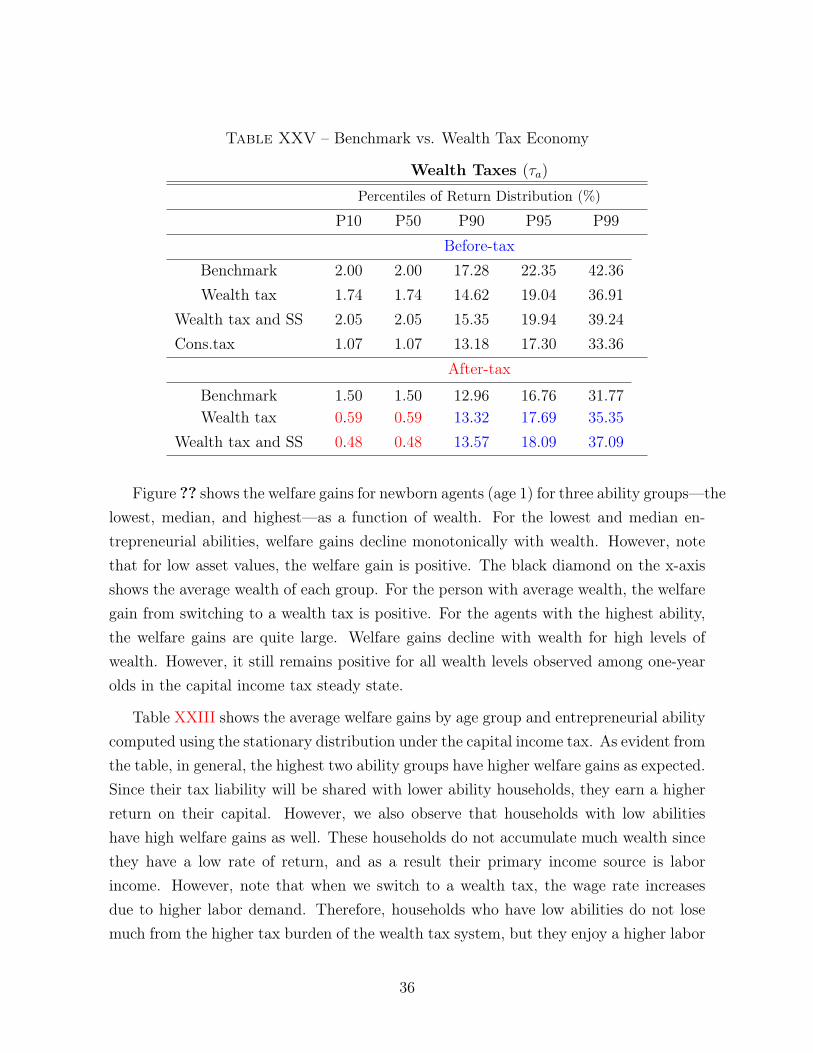
Table XXV – Benchmark vs. Wealth Tax Economy
Wealth Taxes (τa)
Percentiles of Return Distribution (%)
P10 P50 P90 P95 P99Before-tax
Benchmark 2.00 2.00 17.28 22.35 42.36Wealth tax 1.74 1.74 14.62 19.04 36.91
Wealth tax and SS 2.05 2.05 15.35 19.94 39.24Cons.tax 1.07 1.07 13.18 17.30 33.36
After-tax
Benchmark 1.50 1.50 12.96 16.76 31.77Wealth tax 0.59 0.59 13.32 17.69 35.35
Wealth tax and SS 0.48 0.48 13.57 18.09 37.09
Figure ?? shows the welfare gains for newborn agents (age 1) for three ability groups—thelowest, median, and highest—as a function of wealth. For the lowest and median en-trepreneurial abilities, welfare gains decline monotonically with wealth. However, notethat for low asset values, the welfare gain is positive. The black diamond on the x-axisshows the average wealth of each group. For the person with average wealth, the welfaregain from switching to a wealth tax is positive. For the agents with the highest ability,the welfare gains are quite large. Welfare gains decline with wealth for high levels ofwealth. However, it still remains positive for all wealth levels observed among one-yearolds in the capital income tax steady state.
Table XXIII shows the average welfare gains by age group and entrepreneurial abilitycomputed using the stationary distribution under the capital income tax. As evident fromthe table, in general, the highest two ability groups have higher welfare gains as expected.Since their tax liability will be shared with lower ability households, they earn a higherreturn on their capital. However, we also observe that households with low abilitieshave high welfare gains as well. These households do not accumulate much wealth sincethey have a low rate of return, and as a result their primary income source is laborincome. However, note that when we switch to a wealth tax, the wage rate increasesdue to higher labor demand. Therefore, households who have low abilities do not losemuch from the higher tax burden of the wealth tax system, but they enjoy a higher labor
36

% Change in Types in Top x% Wealth GroupTop x% z1 z2 z3 z4 z5 z6 z7 z8 z9
1 -14.81 -11.65 -10.00 -14.98 -10.80 12.59 10.86 6.52 17.395 -5.12 -4.81 -9.89 -6.93 1.58 9.85 8.58 6.35 3.2310 -4.30 -4.52 -8.35 -3.90 2.90 7.48 6.61 5.12 0.0050 -3.28 -3.67 -3.83 0.57 1.76 1.46 1.08 1.17 0.00
(a) Tax Reform from τk to τa: Change in Wealth Composition
% Change in Types in Top x% Wealth GroupTop x% z1 z2 z3 z4 z5 z6 z7 z8 z9
1 -12.76 -11.21 -9.91 -15.51 -11.99 13.30 11.81 6.39 13.045 -4.83 -4.58 -10.15 -7.04 1.48 10.20 8.91 6.45 3.2310 -4.72 -4.61 -9.16 -3.96 3.01 7.94 6.86 4.79 3.1350 -4.34 -4.83 -4.45 0.74 2.10 1.54 0.63 1.14 -2.38
(b) Tax Reform from τk to τa and social security reform: Change in Wealth Composition
% Change in Types in Top x% Wealth GroupTop x% z1 z2 z3 z4 z5 z6 z7 z8 z9
1 -13.99 -11.43 -8.85 -11.88 -7.17 9.43 8.10 4.84 4.355 -7.73 -7.43 -10.07 -6.50 2.31 8.66 7.73 5.59 3.2310 -6.45 -5.93 -7.57 -3.72 3.11 6.48 5.80 3.63 0.0050 -2.26 -2.63 -2.61 0.38 1.14 1.29 1.16 1.05 0.00
(c) Tax Reform from τk to τc: Change in Wealth CompositionFor this we compute the shares under τk and under τa and get the percentage change ofthe shares (not the difference).
income. Households with z3 and z4 have the lowest welfare gains: for the youngest agegroup, welfare gains are 6.8 percent. These are the groups who accumulate relativelymore wealth compared to lower ability groups. Since they obtain a lower after-tax returnunder the wealth tax, they gain the least.
Table XXIV shows the fraction of individuals with a positive welfare gain from thetax reform, by age group and entrepreneurial ability.
Table XXVII summarizes the results from the welfare analysis. The average welfare
37
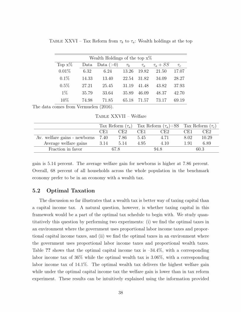
Table XXVI – Tax Reform from τk to τa: Wealth holdings at the top
Wealth Holdings of the top x%Top x% Data Data (>0) τk τa τa + SS τc0.01% 6.32 6.24 13.26 19.82 21.50 17.070.1% 14.33 13.40 22.54 31.82 34.09 28.270.5% 27.21 25.45 31.19 41.48 43.82 37.931% 35.79 33.64 35.89 46.09 48.37 42.7010% 74.98 71.85 65.18 71.57 73.17 69.19
The data comes from Vermuelen (2016).
Table XXVII – Welfare
Tax Reform (τa) Tax Reform (τa)+SS Tax Reform (τc)CE1 CE2 CE1 CE2 CE1 CE2
Av. welfare gains - newborns 7.40 7.86 5.45 4.71 8.02 10.29Average welfare gains 3.14 5.14 4.95 4.10 1.91 6.89
Fraction in favor 67.8 94.8 60.3
gain is 5.14 percent. The average welfare gain for newborns is higher at 7.86 percent.Overall, 68 percent of all households across the whole population in the benchmarkeconomy prefer to be in an economy with a wealth tax.
5.2 Optimal Taxation
The discussion so far illustrates that a wealth tax is better way of taxing capital thana capital income tax. A natural question, however, is whether taxing capital in thisframework would be a part of the optimal tax schedule to begin with. We study quan-titatively this question by performing two experiments: (i) we find the optimal taxes inan environment where the government uses proportional labor income taxes and propor-tional capital income taxes, and (ii) we find the optimal taxes in an environment wherethe government uses proportional labor income taxes and proportional wealth taxes.Table ?? shows that the optimal capital income tax is –34.4%, with a correspondinglabor income tax of 36% while the optimal wealth tax is 3.06%, with a correspondinglabor income tax of 14.1%. The optimal wealth tax delivers the highest welfare gainwhile under the optimal capital income tax the welfare gain is lower than in tax reformexperiment. These results can be intuitively explained using the information provided
38
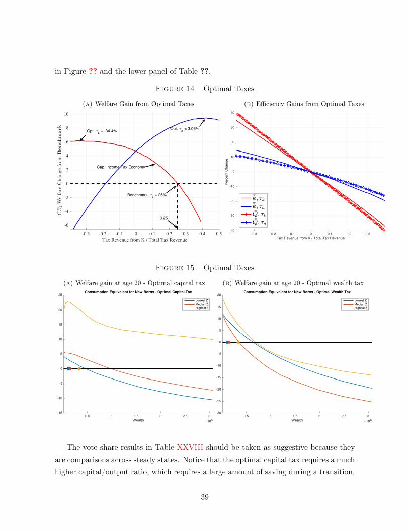
in Figure ?? and the lower panel of Table ??.
Figure 14 – Optimal Taxes
(a) Welfare Gain from Optimal Taxes
-0.3 -0.2 -0.1 0 0.1 0.2 0.3 0.4 0.5
Tax Revenue from K / Total Tax Revenue
-6
-4
-2
0
2
4
6
8
10
CE
2Welfare
Changefrom
Benchmark
Cap. Income Tax Economy
Benchmark, τk = 25%
0.25
Opt. τk = -34.4%
Opt. τa = 3.06%
(b) Efficiency Gains from Optimal Taxes
-0.3 -0.2 -0.1 0 0.1 0.2 0.3
Tax Revenue from K / Total Tax Revenue
-40
-30
-20
-10
0
10
20
30
40
Pe
rcent
Ch
ange
k, τkk, τaQ, τkQ, τa
Figure 15 – Optimal Taxes
(a) Welfare gain at age 20 - Optimal capital tax
0.5 1 1.5 2 2.5 3
Wealth×10
6
-15
-10
-5
0
5
10
15
20
25Consumption Equivalent for New Borns - Optimal Capital Tax
Lowest ZMedian ZHighest Z
(b) Welfare gain at age 20 - Optimal wealth tax
0.5 1 1.5 2 2.5 3
Wealth×10
6
-30
-25
-20
-15
-10
-5
0
5
10
15
20Consumption Equivalent for New Borns - Optimal Wealth Tax
Lowest ZMedian ZHighest Z
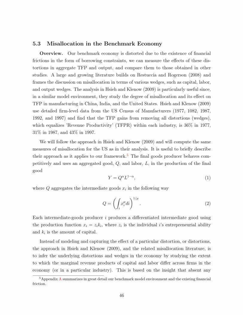
The vote share results in Table XXVIII should be taken as suggestive because theyare comparisons across steady states. Notice that the optimal capital tax requires a muchhigher capital/output ratio, which requires a large amount of saving during a transition,
39
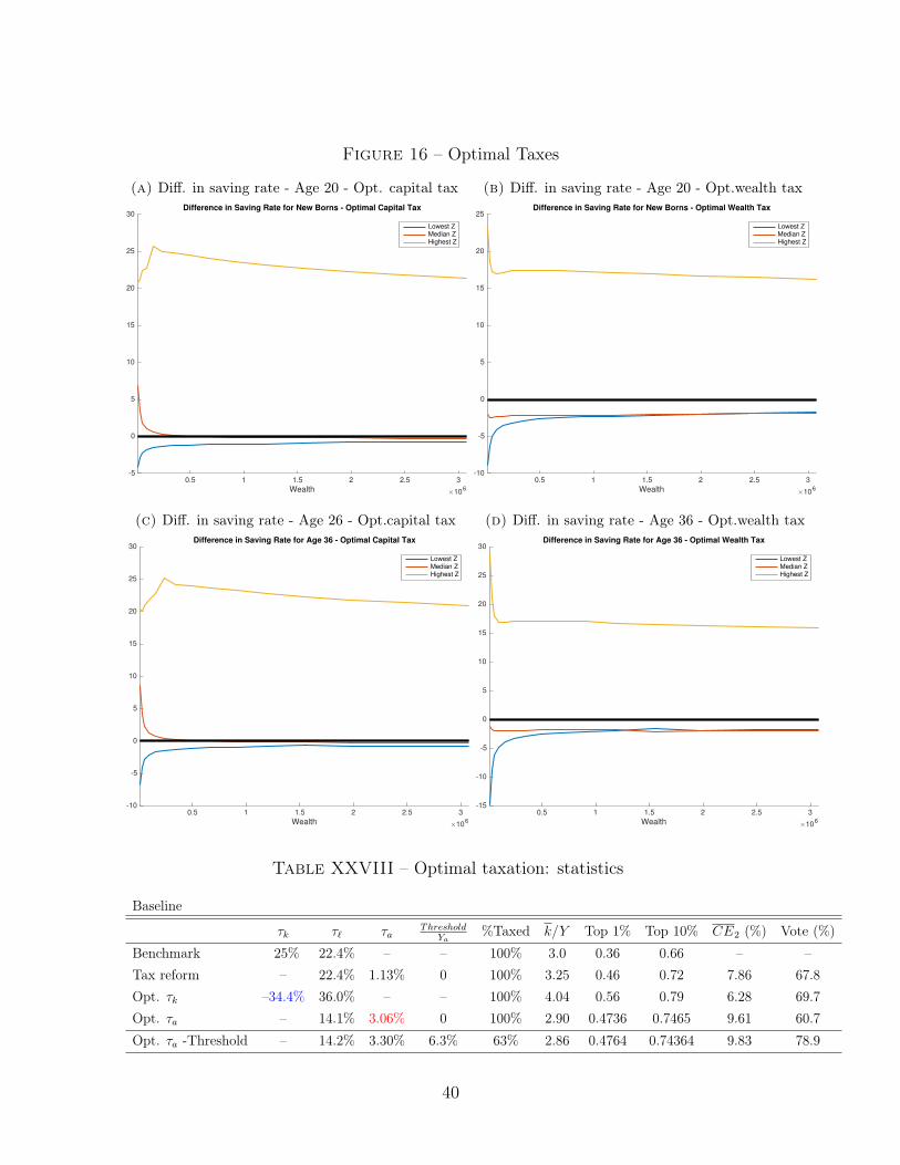
Figure 16 – Optimal Taxes
(a) Diff. in saving rate - Age 20 - Opt. capital tax
0.5 1 1.5 2 2.5 3
Wealth×10
6
-5
0
5
10
15
20
25
30Difference in Saving Rate for New Borns - Optimal Capital Tax
Lowest ZMedian ZHighest Z
(b) Diff. in saving rate - Age 20 - Opt.wealth tax
0.5 1 1.5 2 2.5 3
Wealth×10
6
-10
-5
0
5
10
15
20
25Difference in Saving Rate for New Borns - Optimal Wealth Tax
Lowest ZMedian ZHighest Z
(c) Diff. in saving rate - Age 26 - Opt.capital tax
0.5 1 1.5 2 2.5 3
Wealth×10
6
-10
-5
0
5
10
15
20
25
30Difference in Saving Rate for Age 36 - Optimal Capital Tax
Lowest ZMedian ZHighest Z
(d) Diff. in saving rate - Age 36 - Opt.wealth tax
0.5 1 1.5 2 2.5 3
Wealth×10
6
-15
-10
-5
0
5
10
15
20
25
30Difference in Saving Rate for Age 36 - Optimal Wealth Tax
Lowest ZMedian ZHighest Z
Table XXVIII – Optimal taxation: statistics
Baseline
τk τ` τaThreshold
Ya%Taxed k/Y Top 1% Top 10% CE2 (%) Vote (%)
Benchmark 025% 22.4% – – 100% 3.0 0.36 0.66 – –Tax reform – 22.4% 1.13% 0 100% 3.25 0.46 0.72 7.86 67.8Opt. τk –34.4% 36.0% – – 100% 4.04 0.56 0.79 6.28 69.7Opt. τa – 14.1% 3.06% 0 100% 2.90 0.4736 0.7465 9.61 60.7Opt. τa -Threshold – 14.2% 3.30% 6.3% 63% 2.86 0.4764 0.74364 9.83 78.9
40

which would reduce the welfare benefits and hence the support for the reform. In con-trast, the optimal wealth tax implies a lower capital/output ratio and hence dissaving,so there should be little to no loss during the transition (this is a conjecture!).
Table XXIX – Optimal taxation: Change in variables
Baseline∆K ∆Q ∆L ∆Y ∆w ∆w(net) ∆r ∆r(net) ∆TFP
Tax reform 19.37 24.79 1.28 10.10 8.70 8.70 -0.25 -0.90 4.60Opt. τk 68.97 79.57 –1.16 25.51 26.97 4.72 -1.51 -0.87 6.29Opt. τa 2.76 10.26 3.90 6.40 2.41 13.42 0.68 -1.92 7.29Opt. τa -Threshold 0.41 8.12 3.67 5.42 1.70 12.48 0.78 -2.07 7.70
5.2.1 Welfare Decomposition
Table XXX – Welfare Gain by Age Group and Entrepreneurial Ability - OptimalCapital Taxes
Optimal Capital Taxes
Productivity groupAge z1 z2 z3 z4 z5 z6 z7 z8 z9
20–25 3.7 3.6 3.7 4.9 7.1 10.7 14.8 16.7 17.125–34 3.5 3.4 3.4 4.4 5.9 8.2 10.1 8.9 7.335–44 2.9 2.8 2.7 3.4 4.1 4.7 3.8 1.5 -0.645–54 2.1 2.0 1.9 2.4 2.7 2.6 1.0 -1.1 -3.255–64 0.7 0.7 0.6 1.0 1.2 1.0 -0.2 -2.0 -3.965–74 -0.3 -0.3 -0.3 0.0 0.2 0.1 -0.7 -2.0 -3.575+ -0.1 -0.1 -0.1 0.1 0.2 0.2 -0.3 -1.0 -1.9
41

Table XXXI – Fraction with Positive Welfare Gain by Age Group and EntrepreneurialAbility - Optimal Capital Taxes
Optimal Capital Taxes
Productivity groupAge z1 z2 z3 z4 z5 z6 z7 z8 z9
20–25 0.96 0.95 0.95 0.98 0.99 0.99 0.99 0.99 0.9925–34 0.97 0.97 0.96 0.98 0.97 0.96 0.94 0.90 0.8535–44 0.95 0.94 0.92 0.95 0.93 0.88 0.80 0.68 0.5845–54 0.88 0.88 0.86 0.89 0.85 0.78 0.66 0.53 0.4355–64 0.68 0.67 0.68 0.72 0.69 0.62 0.52 0.41 0.3165–74 0.09 0.05 0.14 0.22 0.22 0.21 0.18 0.15 0.1175+ 0.12 0.12 0.13 0.15 0.15 0.15 0.13 0.11 0.09
Table XXXII – Welfare Gain by Age Group and Entrepreneurial Ability - OptimalWealth Taxes
Optimal Wealth Taxes
Productivity groupAge z1 z2 z3 z4 z5 z6 z7 z8 z9
20–25 11.0 10.7 9.9 9.1 9.2 10.3 12.1 12.4 11.325–34 10.5 10.2 9.1 7.7 6.6 5.7 4.3 -0.1 -5.535–44 8.9 8.6 7.5 5.8 4.1 1.7 -2.4 -8.2 -13.145–54 6.5 6.3 5.4 3.9 2.3 -0.3 -4.6 -9.3 -13.255–64 2.5 2.4 1.8 0.9 -0.1 -2.1 -5.4 -9.1 -12.365–74 -0.7 -0.7 -0.9 -1.3 -1.8 -3.0 -5.3 -7.9 -10.475+ -0.1 -0.1 -0.2 -0.3 -0.6 -1.3 -2.7 -4.5 -6.2
42

Table XXXIII – Fraction with Positive Welfare Gain by Age Group and EntrepreneurialAbility - Optimal WealthTaxes
Optimal Wealth Taxes
Productivity groupAge z1 z2 z3 z4 z5 z6 z7 z8 z9
20–25 0.97 0.97 0.95 0.93 0.93 0.94 0.93 0.90 0.8725–34 0.98 0.98 0.96 0.93 0.90 0.86 0.77 0.59 0.4335–44 0.97 0.97 0.94 0.87 0.80 0.66 0.48 0.35 0.2745–54 0.93 0.93 0.88 0.79 0.68 0.55 0.42 0.32 0.2555–64 0.73 0.72 0.67 0.59 0.51 0.41 0.33 0.25 0.1965–74 0.00 0.02 0.01 0.02 0.01 0.01 0.01 0.00 0.0075+ 0.00 0.00 0.04 0.03 0.02 0.02 0.01 0.01 0.00
Table XXXIV – Welfare Gain by Age Group and Entrepreneurial Ability - OptimalWealth Taxes with Threshold
Optimal Wealth Taxes with Threshold
Productivity groupAge z1 z2 z3 z4 z5 z6 z7 z8 z9
20–25 10.5 10.3 9.8 9.3 9.5 10.6 12.4 12.6 11.425–34 10.1 9.9 9.0 7.8 6.7 5.7 4.2 -0.5 -6.335–44 8.6 8.4 7.4 5.8 4.1 1.5 -2.8 -9.0 -14.245–54 6.3 6.2 5.3 3.9 2.2 -0.5 -5.1 -10.0 -14.255–64 2.5 2.4 1.9 1.0 0.0 -2.1 -5.7 -9.6 -13.065–74 -0.5 -0.5 -0.6 -1.0 -1.5 -2.8 -5.3 -8.2 -10.975+ -0.1 -0.1 -0.1 -0.2 -0.4 -1.1 -2.7 -4.7 -6.5
43

Table XXXV – Fraction with Positive Welfare Gain by Age Group and EntrepreneurialAbility - Optimal Wealth Taxes with Threshold
Optimal Wealth Taxes with Threshold
Productivity groupAge z1 z2 z3 z4 z5 z6 z7 z8 z9
20–25 0.97 0.97 0.95 0.93 0.93 0.94 0.93 0.90 0.8625–34 0.98 0.98 0.96 0.93 0.90 0.85 0.77 0.57 0.4235–44 0.97 0.97 0.94 0.87 0.79 0.66 0.48 0.35 0.2745–54 0.93 0.92 0.87 0.79 0.68 0.55 0.42 0.32 0.2555–64 0.79 0.78 0.74 0.65 0.56 0.46 0.36 0.28 0.2165–74 0.70 0.63 0.65 0.57 0.49 0.42 0.34 0.26 0.2075+ 0.93 0.92 0.90 0.84 0.78 0.68 0.55 0.43 0.34
Table XXXVI – Decomposition of Welfare Gain - CE1
Tax Reform Opt. τk Opt. τaNB All NB All NB All
CE1 7.40 3.14 5.55 2.38 10.03 3.61Cons.Total 7.71 3.71 5.73 2.55 9.91 4.21Level 10.48 10.01 16.88 21.04 10.59 8.28Dist. -2.51 -5.73 -9.55 -15.28 -0.62 -3.76
LeisureTotal -0.29 -0.55 -0.17 -0.17 0.09 -0.59Level -0.52 -0.66 0.31 0.73 -2.13 -2.21Dist. 0.23 0.10 -0.50 -0.90 2.22 1.59
“NB” means new born and “All” is the whole population
44

Table XXXVII – Decomposition of Welfare Gain - CE2
Tax Reform Opt. τk Opt. τaNB All NB All NB All
CE2 7.86 5.14 6.28 4.87 9.61 4.79Cons.Total 8.27 5.58 5.90 4.99 11.02 5.10Level 10.48 10.01 16.88 21.04 10.59 8.28Dist. -2.00 -4.03 -9.40 -13.26 0.38 -2.94
LeisureTotal -0.38 -0.61 0.36 1.10 -1.27 -2.54Level -0.52 -0.66 0.31 0.73 -2.13 -2.21Dist. 0.13 0.02 0.04 0.41 0.67 -0.69
“NB” means new born and “All” is the whole population
45
5.3 Misallocation in the Benchmark Economy
Overview. Our benchmark economy is distorted due to the existence of financialfrictions in the form of borrowing constraints, we can measure the effects of these dis-tortions in aggregate TFP and output, and compare them to those obtained in otherstudies. A large and growing literature builds on Restuccia and Rogerson (2008) andframes the discussion on misallocation in terms of various wedges, such as capital, labor,and output wedges. The analysis in Hsieh and Klenow (2009) is particularly useful since,in a similar model environment, they study the degree of misallocation and its effect onTFP in manufacturing in China, India, and the United States. Hsieh and Klenow (2009)use detailed firm-level data from the US Census of Manufacturers (1977, 1082, 1987,1992, and 1997) and find that the TFP gains from removing all distortions (wedges),which equalizes ’Revenue Productivity’ (TFPR) within each industry, is 36% in 1977,31% in 1987, and 43% in 1997.
We will follow the approach in Hsieh and Klenow (2009) and will compute the samemeasures of misallocation for the US as in their analysis. It is useful to briefly describetheir approach as it applies to our framework.5 The final goods producer behaves com-petitively and uses an aggregated good, Q, and labor, L, in the production of the finalgood
Y = QαL1−α, (1)
where Q aggregates the intermediate goods xi in the following way
Q =
(∫i
xµi di
)1/µ
. (2)
Each intermediate-goods producer i produces a differentiated intermediate good usingthe production function xi = ziki, where zi is the individual i’s entrepreneurial abilityand ki is the amount of capital.
Instead of modeling and capturing the effect of a particular distortion, or distortions,the approach in Hsieh and Klenow (2009), and the related misallocation literature, isto infer the underlying distortions and wedges in the economy by studying the extentto which the marginal revenue products of capital and labor differ across firms in theeconomy (or in a particular industry). This is based on the insight that absent any
5Appendix A summarizes in great detail our benchmark model environment and the existing financialfriction.
46
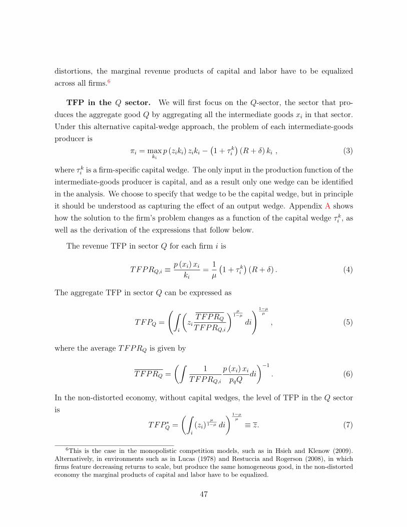
distortions, the marginal revenue products of capital and labor have to be equalizedacross all firms.6
TFP in the Q sector. We will first focus on the Q-sector, the sector that pro-duces the aggregate good Q by aggregating all the intermediate goods xi in that sector.Under this alternative capital-wedge approach, the problem of each intermediate-goodsproducer is
πi = maxki
p (ziki) ziki −(1 + τ ki
)(R + δ) ki , (3)
where τ ki is a firm-specific capital wedge. The only input in the production function of theintermediate-goods producer is capital, and as a result only one wedge can be identifiedin the analysis. We choose to specify that wedge to be the capital wedge, but in principleit should be understood as capturing the effect of an output wedge. Appendix A showshow the solution to the firm’s problem changes as a function of the capital wedge τ ki , aswell as the derivation of the expressions that follow below.
The revenue TFP in sector Q for each firm i is
TFPRQ,i ≡p (xi)xiki
=1
µ
(1 + τ ki
)(R + δ) . (4)
The aggregate TFP in sector Q can be expressed as
TFPQ =
(∫i
(ziTFPRQ
TFPRQ,i
) µ1−µ
di
) 1−µµ
, (5)
where the average TFPRQ is given by
TFPRQ =
(∫1
TFPRQ,i
p (xi)xipqQ
di
)−1. (6)
In the non-distorted economy, without capital wedges, the level of TFP in the Q sectoris
TFP ∗Q =
(∫i
(zi)µ
1−µ di
) 1−µµ
≡ z. (7)
6This is the case in the monopolistic competition models, such as in Hsieh and Klenow (2009).Alternatively, in environments such as in Lucas (1978) and Restuccia and Rogerson (2008), in whichfirms feature decreasing returns to scale, but produce the same homogeneous good, in the non-distortedeconomy the marginal products of capital and labor have to be equalized.
47

Therefore, we can measure the improvement in TFP in the Q sector, ΩQ, as a result ofeliminating the capital wedges, or equivalently, as a result of eliminating the borrowingconstraints:
ΩQ =TFP ∗QTFPQ
=
(∫i
(z
zi
TFPRQ,i
TFPRQ
) µ1−µ
di
) 1−µµ
. (8)
Table XXXVIII reports ΩQ for various economies − the TFP in the Q sector in the non-distorted economy is 58% higher than in the benchmark economy, 51% higher than inthe economy with a wealth tax, 54% higher than in the economy with consumption tax,49% higher than in the economy with an optimal capital income tax, and 47% higherthan in the economy with an optimal wealth tax.
Wealth taxes give the higher TFP gains, allowing for better allocation of capital acrossfirms, even without eliminating the borrowing constraints. The tax reform experimentto wealth taxes implies a TFP gain of 4.6% and optimal wealth taxes give a TFP gainof 7.3% with respect to our benchmark economy.
This can also be seen in the dispersion of TFPR of the different models. Recall thatabsent any constraints on the firms the TFPR would be equated across all of them, sothere is higher misallocation in the economy the higher the dispersion of TFPR acrossfirms. Table XXXVIII reports the standard deviation of TFPR and some of its per-centiles.
Table XXXVIII – Hsieh and Klenow (2009) Efficiency Measure - Benchmark Model
Benchmark Tax Reform (τa) Tax Reform (τc) Opt. Taxes (τk) Opt. Taxes (τa)
TFPQ 1.001 1.047 1.027 1.064 1.074TFP ∗QTFPQ
1.582 1.514 1.543 1.489 1.475Mean TFPR 0.145 0.131 0.12 0.106 0.145StD TFPR 0.054 0.048 0.044 0.039 0.053p99.99 0.94 0.85 0.8 0.69 0.91p99.9 0.68 0.61 0.58 0.5 0.66p99 0.35 0.32 0.3 0.27 0.35p95 0.23 0.2 0.19 0.17 0.23p90 0.19 0.17 0.16 0.14 0.19p75 0.16 0.14 0.13 0.11 0.16p50 0.14 0.12 0.11 0.1 0.14p25 0.12 0.11 0.1 0.09 0.12p10 0.1 0.09 0.08 0.07 0.1p1 0.08 0.07 0.07 0.06 0.09
48
Comparison with the Hsieh and Klenow (2009) results for the US. Inorder to compare these results with the results reported in Hsieh and Klenow (2009) forthe US, we need to use equation (1) and note that the improvement in aggregate output,ΩY , as a result of eliminating the capital wedges in the economy can be expressed as
ΩY =Y ∗
Y=
(TFP ∗QTFPQ
)α(K∗
K
)α(L∗
L
)1−α
. (9)
Since the model with capital wedges is static, the effect of the removal of the capitalwedges on aggregate capital, K, and labor supply, L cannot be taken into account. Theanalysis in Hsieh and Klenow (2009), measures the improvement in total output as aresult of an improvement in TFP in all industries. In our model, this corresponds tothe improvement in TFP in the Q sector. Therefore, removing the capital wedges wouldincrease total output, through its effect on TFP in the Q sector, by 20%.7
Two things are important to point out. First, the magnitude of the misallocation inour benchmark economy is substantial, although a bit lower than the one measured inHsieh and Klenow (2009) using micro data from manufacturing firms: 36% in 1977, 31%in 1987, and 43% in 1997. Our benchmark economy is parametrized based on momentsfrom the entire economy, not just the manufacturing sector. Second, our benchmarkmodel is a dynamic model and any changes in the financial frictions will affect aggregatecapital accumulation and aggregate labor supply. The misallocation calculations abovedo not take those changes into account. It is clear, however, that eliminating the financialfriction would increase the aggregate capital stock K and lead a larger increases in totaloutput than measured above. The effect on aggregate labor supply is less obvious.
7Note that ΩY = ΩαQ = Ω0.40Q = 1.20.
49
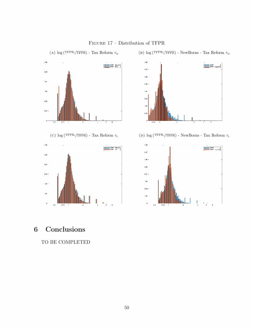
Figure 17 – Distribution of TFPR
(a) log (TFPRi/TFPR) - Tax Reform τw (b) log (TFPRi/TFPR) - NewBorns - Tax Reform τw
(c) log (TFPRi/TFPR) - Tax Reform τc (d) log (TFPRi/TFPR) - NewBorns - Tax Reform τc
6 Conclusions
TO BE COMPLETED
50
References
Aiyagari, Rao S., “Optimal Capital Income Taxation with Incomplete Markets, Bor-rowing Constraints, and Constant Discounting,” Journal of Political Economy, 1995,103 (6), 1158–1175.
Aiyagari, S Rao, “Uninsured Idiosyncratic Risk and Aggregate Saving,” The QuarterlyJournal of Economics, August 1994, 109 (3), 659–84.
Atkeson, Andrew, V. V. Chari, and Patrick J. Kehoe, “Taxing Capital Income:A Bad Idea,” Federal Reserve Bank of Minneapolis Quarterly Review, 1999, 23 (3),3–17.
Benhabib, Jess, Alberto Bisin, and Shenghao Zhu, “The Distribution of Wealthand Fiscal Policy in Economies With Finitely Lived Agents,” Econometrica, 2011, 79(1), 123–157.
, , and , “The Wealth Distribution in Bewley Models with Investment Risk,”Working Paper, 2013.
, , and , “The Distribution of Wealth in the Blanchard-Yaari Model,” Macroeco-nomic Dynamics, Forthcoming, 2014.
Buera, F., J. Kaboski, and Yongseok Shin, “Finance and Development: A Tale ofTwo Sectors,” American Economic Review, August 2011, pp. 1964–2002.
Cagetti, Marco and Mariacristina De Nardi, “Entrepreneurship, Frictions, andWealth,” Journal of Political Economy, 2006, 114 (5), 835–869.
and , “Estate Taxation, Entrepreneurship, and Wealth,” American Economic Re-view, 2009, 99 (1), 85–111.
Castañeda, Ana, Javier Díaz-Giménez, and José-Víctor Ríos-Rull, “Accountingfor the U.S. Earnings and Wealth Inequality,” The Journal of Political Economy, 2003,111 (4), 818–857.
Chamley, Christophe, “Optimal Taxation of Capital Income in General Equilibriumwith Infinite Lives,” Econometrica, 1986, 54 (3), 607–622.
51
Conesa, Juan Carlos, Sagiri Kitao, and Dirk Krueger, “Taxing capital? Not abad idea after all!,” American Economic Review, 2009, 99 (1), 25–48.
Diaz-Gimenez, Javier, Andy Glover, and Jose-Victor Rios-Rull, “Facts on theDistributions of Earnings, Income, and Wealth in the United States: 2007 Update,”Quarterly Review, 2011, (Spr), 2–31.
Erosa, Andres and Martin Gervais, “Optimal Taxation in Life-Cycle Economies,”Journal of Economic Theory, 2002, 105 (2), 338–369.
Gabaix, Xavier, “The Granular Origins of Aggregate Fluctuations,” Econometrica,May 2011, 79-3, 733–772.
Garriga, Carlos, “Optimal Fiscal Policy in Overlapping Generations Models,” mimeo,2003.
Golosov, Mikhail, Narayana Kocherlakota, and Aleh Tsyvinski, “Optimal Indi-rect And Capital Taxation,” Review of Economic Studies, 2003, 70 (3), 569–587.
Guvenen, Fatih, “Learning Your Earning: Are Labor Income Shocks Really Very Per-sistent?,” American Economic Review, June 2007, 97 (3), 687–712.
Hubbard, R. Glenn, Kenneth L. Judd, Robert E. Hall, and Lawrence Sum-mers, “Liquidity Constraints, Fiscal Policy, and Consumption,” Brookings Papers onEconomic Activity, 1986, 1986 (1), 1–59.
Huggett, Mark, “The Risk-Free Rate in Heterogeneous-Agent Incomplete-InsuranceEconomies,” Journal of Economic Dynamics and Control, 1993, 17, 953–969.
Imrohoroglu, Selahattin, “A Quantitative Analysis of Capital Income Taxation,” In-ternational Economic Review, 1998, 39, 307–328.
Jones, Larry E., Rodolfo E. Manuelli, and Peter E. Rossi, “Optimal Taxation inModels of Endogenous Growth,” Journal of Political Economy, 1993, 101 (3), 485–517.
Judd, Kenneth L., “Redistributive Taxation in a Simple Perfect Foresight Model,”Journal of Public Economics, 1985, 28 (1), 59–83.
Kitao, Sagiri, “Labor-Dependent Capital Income Taxation,” Journal of Monetary Eco-nomics, 2010, 57 (8), 959–974.
52
Kocherlakota, Narayana R., “Zero Expected Wealth Taxes: A Mirrlees Approach toDynamic Optimal Taxation,” Econometrica, 2005, 73 (5), 1587–1621.
Krusell, Per and Anthony A Smith, “Income and Wealth Heterogeneity in theMacroeconomy,” Journal of Political Economy, 1998, 106 (5), 867–896.
Lucas, Robert E., “Supply-Side Economics: An Analytical Review,” Oxford EconomicPapers New Series, 1990, 42 (2), 293–316.
Piketty, Thomas, Capital in the Twenty-First Century, Cambridge: Belknap of Har-vard UP, 2014.
Quadrini, Vincenzo, “Entrepreneurship, Saving, and Social Mobility,” Review of Eco-nomic Dynamics, 2000, 3 (1), 1–40.
Shourideh, Ali, “Optimal Taxation of Wealthy Individuals,” Technical Report, Whar-ton School at University of Pennsylvania 2012.
Storesletten, Kjetil, Chris I. Telmer, and Amir Yaron, “The welfare cost of busi-ness cycles revisited: Finite lives and cyclical variation in idiosyncratic risk,” EuropeanEconomic Review, 2001, 45 (7), 1311–1339.
Werning, Ivan, “A Reappraisal of Chamley-Judd Zero Capital Taxation Results,”Working Paper, 2014.
53
A Misallocation in the Benchmark Economy: Details
Production environment
Final Goods Producer. The final goods producer behaves competitively and useslabor and intermediate goods in the production of the final good:
Y = QαL1−α, (10)
where Q is the intermediate good aggregator given by
Q =
(∫i
xµi di
)1/µ
. (11)
The problem of the final good producer can be written as
maxQ,L
QαL1−α − pqQ− wL, (12)
where pq is the price of the intermediate aggregate Q and w is the wage rate.
pq = αQα−1L1−α = αY
Q, w = (1− α)QαL−α = (1− α)
Y
L(13)
The problem of the intermediate good aggregator is
maxxi
pq
(∫i
xµi di
)1/µ
−∫pixidi (14)
Taking the first order conditions, we obtain the following pricing function for intermediategood i
pi (xi) = pq
(∫i
xµi di
) 1−µµ
xµ−1i = pqQ1−µxµ−1i . (15)
Equivalently we can express the price as
p (x) = αxµ−1Qα−µL1−α = pxµ−1 , (16)
54
which satisfies the following relation:
Q =
(∫i
xµi di
)1/µ
Q =
(∫i
((pi (xi)
pq
) 1µ−1
Q
)µ
di
)1/µ
pq =
(∫i
(pi (xi))µµ−1 di
)µ−1µ
Intermediate-good producers. Producer i owns the product line i and produces xiunits of intermediate good i according to
xi = ziki, (17)
where zi is the individual i’s entrepreneurial ability and ki is capital. Entrepreneurialability zi has a permanent and a stochastic component.
Financial markets. There are financial market frictions that restrict the extentto which individuals can borrow to invest in their business. In particular, an individualwith assets a faces a financial constraint
k ≤ ϑ(zi)a,
where ϑ(zi) ∈ [1,∞]. The dependence of ϑ on zi is to allow for the fact that more highlyproductive agents could potentially borrow more with the same level of capital. This is afeature that we will have in the baseline calibration and will also consider the case withϑ(zi) = ϑ. When ϑ = 1 the financial constraint is extreme since the individual can onlyuse her own assets in production. When ϑ =∞ there is no longer a financial constraintsince there is no longer a restriction on the amount that an individual can borrow.
Profit maximization. The individual intermediate good producer seeks to maxi-mize profits
πi = maxki∈(0,ϑ(zi)ai)
p (ziki) ziki − (R + δ) ki .
55
The solution is to set ki equal to
ki = min
ϑ (zi) ai,
(µpzµiR + δ
) 11−µ
.
Wedges and financial frictions
In the benchmark model, the financial friction is explicitly modeled. Alternatively,distortions can be introduced in the model through a capital wedge. In that case theproblem for each firm is
πi = maxki
p (ziki) ziki −(1 + τ ki
)(R + δ) ki . (18)
The optimal level of capital is then
k∗i =
(µpzµi(
1 + τ ki)
(R + δ)
) 11−µ
. (19)
Using the benchmark model, we can obtain the firm-specific capital wedges τ ki as
(1 + τ ki
)=µp (zik
∗i )µ
(R + δ) k∗i. (20)
This solution for the optimal level of capital also allows us to compute the price andoutput of each intermediate good as a function of the capital wedge:
p∗i =1
µ
(1 + τ ki
)(R + δ)
zi(21)
x∗i = zik∗i =
(µpzi(
1 + τ ki)
(R + δ)
) 11−µ
∝(
zi1 + τ ki
) 11−µ
(22)
Misallocation measure
The marginal revenue product of capital for firm i in sector Q is
MRPKQ,i =∂p (ziki) ziki
∂ki= µpzµi k
µ−1i , (23)
56

and firm optimization implies that
MRPKQ,i =(1 + τ ki
)(R + δ) . (24)
The average marginal revenue product of capital in the Q sector is obtained by using asweights the revenue of each firm in the Q sector relative to the total value of output inthe Q sector:
MRPKQ =
∫ (MRPKQ,i
pixipqQ
)di (25)
Two other useful concepts are the individual firm’s physical productivity
TFPQi =xiki
= zi , (26)
and the individual firm’s revenue productivity
TFPRQ,i =p (xi)xiki
= pzµi kµ−1i =
1
µ
(1 + τ ki
)(R + δ) . (27)
A measure of the aggregate TFPRQ can be obtained by noting that TFPRQ,i =1µMRPKQ,i. That implies that
TFPRQ =1
µMRPKQ (28)
We can now proceed with defining the aggregate TFP in the Q sector, TFPQ, by notingthat
Q = TFPQ ·K ,where K =
∫ki di . (29)
We first need to define K. Using the FOC of the individual firm we have:
µpzµi kµi =
(1 + τ ki
)(R + δ) ki
µpxµ−1i xi =(1 + τ ki
)(R + δ) ki
µpixi =(1 + τ ki
)(R + δ) ki
µpixi = MRPKQ,iki
57

which implies that
ki =µpixi
MRPKQ,i
.
We can use this expression to obtain an expression for the aggregate level of capital:
K =
∫kidi =
∫µpixi
MRPKQ,i
di = µpqQ
∫1
MRPKQ,i
pixipqQ
di =µpqQ
MRPKQ
. (30)
Reorganizing we get:pqQ
K=
1
µMRPKQ = TFPRQ . (31)
Then
TFPQ =Q
K
=pqQ
K
1
pq
= TFPRQ1
pq.
Recall that
pq =
(∫i
(pi (xi))µµ−1 di
)µ−1µ
=
∫i
(1
µ
(1 + τ ki
)(R + δ)
zi
) µµ−1
di
µ−1µ
=
(∫i
(TFPRQ,i
zi
) µµ−1
di
)µ−1µ
.
Finally
TFPQ =
(∫i
(ziTFPRQ
TFPRQ,i
) µ1−µ
di
) 1−µµ
(32)
which is our measure of TFP.
If capital were allocated efficiently across firms then the marginal revenue product of
58
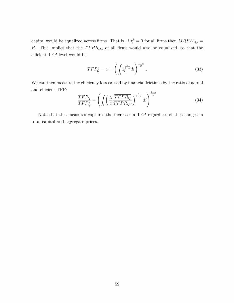
capital would be equalized across firms. That is, if τ ki = 0 for all firms thenMRPKQ,i =
R. This implies that the TFPRQ,i of all firms would also be equalized, so that theefficient TFP level would be
TFP ∗Q = z =
(∫i
zµ
1−µi di
) 1−µµ
. (33)
We can then measure the efficiency loss caused by financial frictions by the ratio of actualand efficient TFP:
TFPQTFP ∗Q
=
(∫i
(ziz
TFPRQ
TFPRQ,i
) µ1−µ
di
) 1−µµ
(34)
Note that this measures captures the increase in TFP regardless of the changes intotal capital and aggregate prices.
59