Embed Size (px)
Citation preview

Use of Wavelets and Filter Banks in 2D Gel
Electrophoresis Images in Spot Picker Robot for Precise
Protein Identification
By
Ratnesh Singh Sengar
< ENGG01201004024>
Bhabha Atomic Research Centre, Mumbai
A thesis submitted to the
Board of Studies in Engineering Sciences
In partial fulfillment of requirements
for the Degree of
DOCTOR OF PHILOSOPHY
of
HOMI BHABHA NATIONAL INSTITUTE
February, 2017


STATEMENT BY AUTHOR
This dissertation has been submitted in partial fulfillment of requirements for an advanced
degree at Homi Bhabha National Institute (HBNI) and is deposited in the Library to be made
available to borrowers under rules of the HBNI.
Brief quotations from this dissertation are allowable without special permission, provided
that accurate acknowledgement of source is made. Requests for permission for extended
quotation from or reproduction of this manuscript in whole or in part may be granted by the
Competent Authority of HBNI when in his or her judgment the proposed use of the material is in
the interests of scholarship. In all other instances, however, permission must be obtained from
the author.
(Ratnesh Singh Sengar)

DECLARATION
I, hereby declare that the investigation presented in the thesis has been carried out by me.
The work is original and has not been submitted earlier as a whole or in part for a degree /
diploma at this or any other Institution / University.
(Ratnesh Singh Sengar)

COURSES and PUBLICATIONS
Courses Completed

List of Publications arising from the thesis
Journal
1. “Analysis of 2D-Gel Images for Detection of Protein Spots Using a Novel Nonseparable Wavelet
Based Method”, Ratnesh Singh Sengar, A. K. Upadhyay, M. Singh, V. M. Gadre, Biomedical
Signal Processing and Control(Elsevier journal), vol. 25, 2016, pp. 62-75,
doi:10.1016/j.bspc.2015.10.013.
2. “Protein Spot Extraction in 2D Gel Images Using Sign of Wavelet Coefficients”, Ratnesh Singh
Sengar and V.M.Gadre. (Communicated)
Chapters in books and lectures notes
1. “Wavelet and Fractals in Earth Science”, Chapter-4: Multiscale Processing-A Boon for Self-
similar Data, Data Compression, Singularities and Noise Removal", Ratnesh Sengar,
Venkateswarao Cherukuri, Arpit Agrawal and Vikram M. Gadre, CRC Press, Taylor & Francis
Group, 2013.
Conferences
1. “Approaches based on nonseparable filter banks in 2D Gel electrophoresis image analysis”,
Ratnesh Singh Sengar, A. K. Upadhyay, P. G. Patwardhan, M. Singh, V. M. Gadre, Proceedings
of Asia Pacific Signal and Information Processing Association (APSIPA) International
Conference, Biopolis, Singapore, 2010, pp. 387-392, www.scopus.com/inward/record.url?eid=2-
s2.0-79958151381&partnerID=40&md5=a0 de44adfbb291971da479e13af6e41c.
2. “Segmentation of two-dimensional electrophoresis gel image using the wavelet transform and the
watershed transform “, Ratnesh Singh Sengar, A. K. Upadhyay, M. Singh, V. M. Gadre, The
eighteenth annual National Conference on Communications (NCC-2012), (3-5 Feb. 2012),
DOI:10.1109/NCC.2012.6176861.
3. "Development of Spot Picker Robot for Proteomics Applications", Ratnesh S Sengar,
A.K.Upadhyay, D.N.Badodkar, R.K.Puri, Manjit Singh, MGR Rajan, Vikram M Gadre, IEEE
International Conference on Robotics & Automation (IEEE-ICRA2013) at Karlsruhe, Germany,
2013, pp 1704-1709, DOI: 10.1109/ICRA.2013.6630801.
Workshop
1. "Wavelets: Data Processing across Scales", Ratnesh S Sengar, Venkateshwararao Cherukuri,
Satyaprakash Pareek, Arpit Agarwal, Vikram M. Gadre, National Workshop on Wavelets,
Multiresolution and Multifractal Analyses in Earth, Ocean and Atmospheric Sciences - Current
Trends (WMMFA-2012), Session I, IIT, Bombay, Mumbai, February 29 - March 2, 2012.
(Ratnesh Singh Sengar)

Dedicated to my Parents

ACKNOWLEDGEMENTS
I would like to thank my guide, Prof. (Dr.) V. M. Gadre, Department of Electrical
Engineering, IIT-Bombay for giving me the opportunity to pursue a PhD and for his excellent
supervision, practical help, unabated inspiration, valuable suggestions and most untiring help at
all stages, which has helped me to complete this project in the present form. I am particularly
grateful to my office supervisors and technical advisor, Mr. Manjit Singh, Ex Director, DMA
Group and Dr. D. N. Badodkar, Distinguish Scientist, Associate Director, DMAG & Head,
DRHR for lending me their understanding, constructive guidance and support during my course
work at IIT-Bombay. I would also like to thank my immediate supervisor Mr. R. K. Puri for his
constant support and encouragement to complete my PhD work. A special thanks to Dr. Kallol
Roy, Dr. Archana Sharma and other members of the Doctorate committee for giving me
extremely helpful and logical suggestions, and everyone in my department (DRHR) for making
this a very enjoyable time. I also extend my sincere thanks to Dr S. Mukhopadhyay, Head,
Siesmology Division for useful suggestions and available for all the worthful discussions. I am
extremely thankful to our DRHR, BARC colleagues Mr. A.K Upadhyay and Mr. Rohit Sharma,
who gave their time and insight for the successful completion of my thesis. I would also like to
thank Prof. Sanjeeva Srivastva, Biosciences & Bioengineering, IIT-Bombay, Dr. MGR Rajan
(RMC, BARC), Dr. H.S.Mishra (MBD, BARC) and Dr. Bhakti Basu (MBD, BARC) for
providing me with the required assistance and the gel images that were used in this thesis. I
would like to thank the students of Electrical Engineering Department, IIT-Bombay who have
contributed their time in helping me with this thesis and for fruitful discussions and critical
review.

Finally, I would like to express my sincere gratitude to my wonderful parents for their love
and support throughout the whole project. I would like to thank my wife Jaya for standing beside
me during this project. I also thank my lovely children Swastika and Suryaansh for always
making me smile and for understanding on those weekend morning when I was working on this
project instead of spending time with them. A special thanks to my sister Rashmi for devoting
her time and efforts with the editing of the thesis and providing insight to make it more
meaningful.

Contents Abstract ........................................................................................................................................................ iv
List of Figures ................................................................................................................................................ v
List of Tables ................................................................................................................................................. x
Chapter 1 Introduction ................................................................................................................................. 1
1.1 Motivation ........................................................................................................................................... 1
1.2 The virtue of Proteomics ..................................................................................................................... 2
Two-Dimensional Gel Electrophoresis in Proteomics ............................................................................... 2
1.3 Spot Picker Robot ................................................................................................................................ 7
1.3.1 Illumination System ..................................................................................................................... 7
1.3.2 Spot Cutting Tool.......................................................................................................................... 9
1.3.3 Robotic System............................................................................................................................. 9
1.3.4 Control System and Software .................................................................................................... 10
1.3.5 Image Analysis of 2DGE Images ................................................................................................. 11
1.4 Literature for 2DGE Images Analysis ................................................................................................. 16
1.5 Problems Addressed in This Thesis ................................................................................................... 18
1.5.1 Contribution of This Thesis ........................................................................................................ 19
Chapter 2 Multi-Scale Processing and Nonseparable Wavelets ................................................................. 22
2.1 Introduction ...................................................................................................................................... 22
2.2 Dyadic Multiresolution Analysis (MRA) ............................................................................................ 23
2.2.1 Axioms of Dyadic MRA ............................................................................................................... 24
2.2.2 Theorem of MRA ........................................................................................................................ 27
2.3 Singularities and Noise behavior....................................................................................................... 29
2.3.1 Singularities ................................................................................................................................ 29
2.3.2 Wavelets in Singularity Detection .............................................................................................. 30
2.4 Nonseparable Wavelet...................................................................................................................... 33
2.4.1 Building Blocks of Multi-rate System ......................................................................................... 35
2.5 Quincunx Wavelet Transform ........................................................................................................... 41
2.6 Lifting Scheme ................................................................................................................................... 44
Chapter 3 Denoising Of 2DGE Images ......................................................................................................... 48
3.1 Introduction ...................................................................................................................................... 48

3.2 Denoising Techniques ....................................................................................................................... 49
3.3 Wavelet Shrinkage Method .............................................................................................................. 50
3.3.1 Motivation for Wavelet Shrinkage ............................................................................................. 50
3.3.2 Thresholding: Soft and Hard ...................................................................................................... 52
3.3.3 Image Denoising Algorithm ........................................................................................................ 53
3.3.4 Threshold Determination ........................................................................................................... 53
3.4 Image Denoising: A Wavelet Domain Modeling Approach ............................................................... 56
3.4.1 Stochastic Model for Wavelet Coefficient ................................................................................. 57
3.5 Use of Nonseparable Wavelet .......................................................................................................... 62
3.6 Evaluation Methodology ................................................................................................................... 62
3.6.1 PSNR Based Analysis on Synthetic Images ................................................................................. 64
Chapter 4 Segmentation of Low-resolution 2DGE Images ......................................................................... 72
4.1 Introduction ...................................................................................................................................... 72
4.2 Method using Wavelet Transform and Watershed Transform ........................................................ 74
4.2.1 Watershed Transform and Problems ......................................................................................... 74
4.2.2 Proposed Segmentation Method ............................................................................................... 75
4.2.3 Experiments and Results ............................................................................................................ 79
4.3 Method using Wavelet Interscale Ratios .......................................................................................... 82
4.3.1 Proposed Image Model .............................................................................................................. 83
4.3.2 Image Decomposition ................................................................................................................ 83
4.3.3 LMMSE Based Denoising ............................................................................................................ 83
4.3.4 Discrimination Power of the Wavelet Coefficients .................................................................... 85
5.3.5 Discrimination among Spot Region, Edge and Background ....................................................... 87
4.3.6 Texture Characterization and Spot Detection ........................................................................... 90
4.3.7 Energy Distribution Model ......................................................................................................... 94
4.3.8 Oversaturated Spots .................................................................................................................. 96
4.3.9 Overall Strategy .......................................................................................................................... 99
4.3.10 Experimental Results and Discussions ................................................................................... 100
Chapter 5 Segmentation of High-resolution 2DGE Images ....................................................................... 112
5.1 Introduction .................................................................................................................................... 112
5.2 Method using Wavelet and Kernel Density Estimation (KDE) ........................................................ 112
5.2.1 Foundation ............................................................................................................................... 113

5.2.2 Wavelet and Blob Regions ....................................................................................................... 117
5.2.3 Proposed Method .................................................................................................................... 120
5.2.4 Region Refinement................................................................................................................... 123
5.2.5 Experimental Results and Discussion ....................................................................................... 129
5.2.6 Detailed Results on Synthetic Image ....................................................................................... 142
Conclusion ................................................................................................................................................. 148
Appendix I 2DGE Image Registration ........................................................................................................ 150
I.1 Introduction ..................................................................................................................................... 150
I.2 Registration Techniques ................................................................................................................... 151
I.2.1 Intensity Based .......................................................................................................................... 151
I.2.2 Point Set Registration ............................................................................................................... 153
References ................................................................................................................................................ 157

Abstract The main aim of this thesis is to bring in novel advanced techniques for the analysis of two-
dimensional gel electrophoresis (2DGE) images, to provide more accurate protein spot detection
in the field of proteomics. 2DGE is an important and the most widely used technique for
analyzing protein expression in this field. By this technique, a very large number of proteins can
easily and simultaneously be separated, identified and characterized. Due to very tedious and
laborious work involved in the separation of thousands of proteins, a completely automated
integrated system for the analysis of 2DGE images and spot excision is increasingly in demand.
The nature of 2DGE images poses some great challenges, such as very noisy and inhomogeneous
background with several irregular protein spots. These irregular protein spots are of varying size,
shape and intensity. In this Thesis, problems of noise removal and methods of image
segmentation are addressed to solve various challenges, such as faint or weak spots, overlapped
spots and streaks, to a great extent. These challenges lead us to develop three novel segmentation
methods; each method provides different insights into the problem and exhibits significant
improvements over the available commercial software and methods for 2DGE images.
The main contribution of the proposed algorithms is the use of nonseparable wavelets to
study the nature of protein spots in the scale-space paradigm and to formulate efficient strategies
for recognition. The first method analyzes the difference between streaks and spots, which are
characterized in a nonseparable wavelet domain and combined with the watershed method for
complete segmentation. In the second method, we have devised a technique to find out the faint
spots by using inter-scale ratios of the wavelet coefficients. This technique is based on a single
threshold and is independent of the gray value of the image. It copes with the inhomogeneities in
the 2DGE images up to a large extent, which is helpful for finding the protein spots accurately.
The third method emphasizes the minimization of artifacts and actual blob region identification
in the noisy inhomogeneous background, by using kernel density estimation technique in the
nonseparable wavelet domain.

List of Figures
1.1 Laboratory process of making of 2DGE image 6
1.2 1D gel image 6
1.3 2D gel images 6
1.4 Spot Picker Robot 8
1.5 Typical flow of gel-based proteomics 8
1.6 Illumination Source 9
1.7 Spot Cutting Tool 9
1.8 Computer based control system for Spot Picker Robot 10
1.9 Spot cut from the gel (a) by Spot Picker Robot (b) by manual operation 11
1.10 Different types of protein spots 12
1.11 (a) A typical 2DGE image with varying background (b) Intensity line profile 13
1.12 a) Foreground intensity histogram (range covered 0-253) 14
b) Background intensity histogram (range covered 20-255) 15
c) Gel image histogram 15
2.1 Illustration of Ladder Axiom 25
2.2 Types of Singularities 29
2.3 Retention of singularities across the scales 31
2.4 Illustration of noise removal using ‘db8’: (a) original signal, (b) signal with additive
random noise, (c) detail coefficients at scale 1, (d) detail coefficients at scale 2 and
(e) detail coefficients at scale 3
32
2.5 Division of frequency region with 2D two channels separable filter banks, (a)
vertical, (b) horizontal [34]
35
2.6 Lattice generated by Quincunx matrix 36
2.7 (a) Before down-sampling, (b) Down-sampling by Quincunx matrix 37
2.8 (a) Based-band region (b), (c) and (d) three aliases for decimation matrix M 38
2.9 Decimation 39
2.10 Up-sampling using matrix M (a) (a) Input signal (b) Up-sampled signal 39
2.11 Interpolator 40
2.12 Perfect reconstruction filter bank 40
2.13 The Quincunx lattice (shaded point shows lattice points) 43
2.14 Quincunx filter bank 44

2.15 Frequency supports of filters in Quincunx filter bank 44
2.16 Lifting Structure for Quincunx filter Bank in (a)-Analysis and (b)-Synthesis 47
3.1 (a) Original signal with singularities (in black) and noisy signal (in yellow)
(b) histogram of magnitude of `db6' wavelet coefficients of noisy signal
51
3.2 (a) Hard thresholding (b) Soft thresholding 52
3.3 (a) Original Image (b) Corrupted by Gaussian noise (c) Denoised by VisuShrink (d)
Denoised by SUREshrink (e) Denoised by BayesShrink
56
3.4 (a) Histogram of the high-band wavelet coefficients of gel Image (b) Blue line:
histogram of the same coefficients scaled by estimated local standard deviations.
Red line: unit-variance, zero-mean Gaussian pdf
58
3.5 A 2DGE image from database [1] 59
3.6 (a) Block diagram of the denoising algorithm (b) Histogram of the estimated local
variance of the coefficients(solid line) in wavelet image sub-band, approximated
using a single exponential prior (dash-dotted line) and a mixture of exponentials
that consists of three single exponentials in three non-overlapping regions (dashed
line)
60
3.7 Histograms of Quincunx wavelet coefficients of various sub-bands of the 2DGE
image in Figure 3.7 (a) Level-1 Scale-1 (b) Level-1 Scale-2 (c) level-2 Scale-1(d)
Level-2 Scale-2
63
3.8 (a) Clean synthetic image (b) Noisy image-1(σ=30) (c) Noisy image-2 (σ=35) (d)
Noisy image-3(σ=40)
64
3.9 Denoised Synthetic Images using (a) CWT with BayesShrink (b) Quincunx with
BayesShrink (c) Coif5 with Bayes shrink (d) Db8 with BayesShrink (e) Statistical
Model on Quincunx coefficients with 7x7 window (MAP rule) (f) Statistical Model
on db8 coefficients with 7x7 window(MAP rule)
70
3.10 3D view of synthetic images. 71
3.11 De-noised images are processed through Delta 2D package. Segmented images are
shown. (a) image denoised by coiflet and processed. Total 412 spots are detected
out of 457 true spots. (b) image denoised by quincunx and processed. Total 446
spots are detected out of 457 true spots.
71
4.1 Block diagram of proposed segmentation approach 80
4.2 Segmented Spots 81
4.3 A part of gel image showing some missing spots and false spots using Delta2D and
using the proposed method
81
4.4 The histogram of the wavelet coefficients is plotted along with a Gaussian curve
for comparison and measurement of DP values
85
4.5 The pdf of IDI and two threshold levels T1 and T2 88
4.6 A real 2D gel image with protein spots (left) and corresponding IDI values (right).
The dark colors indicate low values and bright colors indicate high values
88
4.7 The tricolor image of IDI values of the protein spots (right) with corresponding
original image (left). Black colors indicates interiors (IDI<T1), white color indicates
edges (IDI>T2) and gray color indicates background (T1<IDI<T2).
89
4.8 The oversaturated spots (left) and corresponding IDI values (right). In right image,
bright color indicates high IDI values
90
4.9 (a) The edge information from IDI (IDI>T2) is overlaid on the corresponding part of
the real gel image. (b) The interior information (IDI < T1) is overlaid on the same
part of the real gel image
90
4.10 (a) An original 2D gel image with (b) its ITP, (c) its binary image made by ITP >=0.02
and (d) its binary image obtained using global 2D Otsu threshold on gray value
image
93
4.11 (a) A 2D gel image. (b), (c) and (d) its binary images obtained through applying
different gray value thresholds (b) 100 (c) 75 and (d) 25 respectively
94
4.12 3D profile of ITP of a typical faint spot 94
4.13 (a) An oversaturated spot with multiple regional maxima of ITP on its boundary. (b)
The segmentation of the overlapped oversaturated spots
97
4.14 Effect of different values of ITPMIN on the segmentation result of a real gel image.
(a) ITPMIN = 1% (b) ITPMIN = 2% (c) ITPMIN = 5% and (d) ITPMIN = 10%. Spots identified
as oversaturated spots are depicted with green border and the rest of spots are
depicted with pink border
103
4.15 (a) a real gel image from public dataset [77] and segmentation results using (b)
Proposed method (c) ImageMaster 7 and (d) SCIMO
104
4.16 A part of the image and results shown in Figure 5.15(b, c, d) is selected and
zoomed for better visibility. (a) Result by Proposed method (b) Result by
ImageMaster 7 and (c) Result by SCIMO
105
4.17 (a) A synthetic image and its segmentation using (b) Proposed method (c)
ImageMaster 7 and (d) SCIMO
106
4.18 (a) A synthetic image and its segmentation results using (b) Proposed method (c)
ImageMaster 7 and (d) SCIMO
107
4.19 Mean error in spot area overlap between the segmentation method and ground
truth. The error bar indicates the standard deviation of the corresponding measure
(%) across images in dataset
109
4.20 Effect of different amounts of Gaussian noise on the segmentation results of the
methods.
110
5.1 (a) A synthetic image of flat objects. (b) A synthetic 2D Gaussian blob image. (c) A
noise free synthetic dark flat top Gaussian blob image
114
5.2 Hessian Analysis of a noise free and noisy synthetic image at different scales: σ=2
(first row) and σ = 6 (second row). (a) Noise free image at specified resolution (b)
Hessian minima (regions satisfying condition: det(H(x,y; σ)) > 0 and trace(H(x,y;
σ))>0) for noise free image (c) positive Hessian trace (regions satisfying condition:
trace(H(x,y; σ))>0) for noise free image (d) Hessian minima for noisy image (e)
118

positive Hessian trace for noisy image
5.3 Blob regions obtained using Hessian Analysis at different scales for the noise free
and noisy synthetic image. The region of each blob is obtained at its corresponding
scale by searching in the scale range of σ = 2 to σ = 16 in step of 0.5. (a) Original
noise free synthetic image and (b) blob regions obtained for noise free image (c)
noisy synthetic image and (d) blob regions obtained for noisy image
118
5.4 Lifting scheme for undecimated quincunx wavelet: (a) analysis and (b) synthesis.
Predict (P) and update (U) filters are upsampled by dilation matrix D. I1 and D1
represents the approximation and detail part of the next scale and Î represents the
reconstructed image. P2 and U2denotes the second order filters are used [70]
120
5.5 Effect of selection of kernel bandwidth on the obtained binary region. (a) Original
synthetic images and obtained binary regions using proposed method at following
kernel bandwidths: (b) h = 1 (c) h = 6 and (d) h = 10
124
5.6 Pseudo code of the Region Refinement method 127
5.7 Pseudo code for separation of overlapped spots in 2D gel image 128
5.8 (a) Protein spots from original image and separation of overlapped spots after
segmentation, using (b) Euclidian distance, (c) regional minima and (d) proposed
approach
129
5.9 Effect of the parameter RN on the final segmentation. (a) A 2D gel image and (b)-
(e) segmented results using our method when RN was set to 2, 5, 10 and 15
respectively. As value of RN increases, region of blobs spreads out and may merge
nearby blobs. It leads to more global segmentation. (f) Segmentation by a global
method – active contour [7]
133
5.10 Plot of kernel bandwidth (h) vs. average segmentation accuracy SA (%) for six
synthetic images. Images are corrupted with Gaussian noise (with a standard
deviation between 1 and 5) and salt and pepper (1%-3%).Solid line represents
average SA for all mages
134
5.11 Original synthetic/ real images (first row) and segmentation results obtained using
proposed approach ( second row)
135
5.12 (a) A synthetic image consisting 2D Gaussian blobs and its segmentation results
using (b) the proposed approach, (c) watershed method, (d) Otsu’s threshold, (e)
Delta2D and (f) ImageMaster 7
137
5.13 Boundaries of the spots are assumed at a distance of two standard deviations from
their center
137
5.14 Comparison of different segmentation methods for synthetic Gaussian blob
images. (a) The segmented spot regions are evaluated using the terms JD and SA.
(b) The number of segmented spots is evaluated as fraction of the total number of
true spots in ground truth
139
5.15 (a) Real 2D gel sub-image and segmentation results using (b) proposed approach,
(c) watershed, (d) Otsu’s threshold, (e) Delta2D and (f) ImageMaster 7
140
5.16 (a) Real 2D gel sub-image and segmentation results using (b) proposed approach, 141

(c) watershed, (d) Otsu’s threshold, (e) Delta2D and (f) ImageMaster 7
5.17 Segmentation errors for the image of Fig. 5.21(a) with different methods. The
horizontal axis represents the standard deviation of Gaussian noise in the image
145
5.18 Comparison with other state-of-the-art methods 146
5.19 First Row: CV method on synthetic and real 2D gel images. Second Row: KWFCM
method on the same synthetic and real 2D gel images
147
5.20 (a) An image from the public database and its segmentation using (b) our approach
(c) CV and (d) KWFCM
147

List of Tables
Table 1.1 Proposed segmentation methods ............................................................................................... 20
Table 3.1 Mean PSNR values for our set of synthetic images with noise variance 40 ............................... 66
Table 3.2 Mean PSNR values for our set of synthetic images with noise variance 35 ............................... 67
Table 3.3 Mean PSNR values for our set of synthetic images with noise variance 30 ............................... 68
Table 3.4 Comparison of denoising methods for synthetic images ............................................................ 69
Table 4.1 Results in terms of ‘spot efficiency’ ............................................................................................ 82
Table 5.1 Detailed result on synthetic image ........................................................................................... 143
1
Chapter 1 Introduction
1.1 Motivation
Proteomics is the field which involves study of multi-protein systems, focusing on the
interplay of multiple proteins as functional components in a biological system. Two-dimensional
gel electrophoresis (2DGE) is an important and the most widely used technique of analyzing
protein expression in this field. By this technique, a very large number of proteins can easily and
simultaneously be separated, identified and characterized. The detailed study of proteins in this
manner is very useful to analyze earlier protein databases and compare them against the new
proteins which are responsible for making new biomarkers, which helps in diagnosing specific
diseases like cancer. Separating thousands of protein spots is a very tedious and laborious job.
Protein spots are highly irregular in terms of their shape, size and intensity, which make their
automated detection very challenging. Hence, a completely automated system for the analysis of
2DGE images is increasingly in demand.
We have developed the “Spot Picker Robot”, which automates the excision of the protein
spots from 2D gels (up to a size format of 220 mm x 240 mm) obtained from electrophoresis
process for screening of a large number of proteins. Spots can be picked from fluorescent,
coomassie blue or silver stained gels. The spot picker system is capable of imaging as well as
direct picking of protein spots with the help of a 3-axes robotic system.
It is a very challenging task to find out the correct position coordinates of all the proteins in a
2D gel because proteins change their position in each experiment, according to their mass and
charge and also contain a large amount of noise and non-uniform background. The precise

2
excision of correct protein spots is crucial for further analysis. After processing the gel image,
the system generates the spot position coordinates and spot picking list, which are the reference
coordinates of each dynamic protein spot, this is then directly interfaced with the robotic system
for automated protein spot excision. Detection and interpretation of protein spots depend on the
accuracy and reliability of the image processing methods. In this dissertation, the emphasis has
been on proposing solutions to cater the challenges involved in noise removal and protein spot
segmentation of 2DGE images.
The thesis describes and proposes solutions to some of the current challenging problems in
image analysis of two-dimensional gel electrophoresis (2DGE) images. 2DGE is the leading
technique to separate individual protein in plant cells and human cells for drugs and new
biomarkers development. This technique results in an image, where the proteins appear as dark
spots on a bright background. However, the analysis of these images is time-consuming and
requires a large amount of manual work. A lot of commercial software is available which is
mostly based on spatial filtering, and hence, none of it is capable of detecting all the true protein
spots in 2DGE images. So our main objective is to develop robust and fast methods based on
image analysis techniques to detect all the true protein spots, in order to significantly accelerate
this technology.
1.2 The virtue of Proteomics
Two-Dimensional Gel Electrophoresis in Proteomics
Proteomics is becoming an increasingly important part of cell biology and it aims to
understand the basic principles of life “how the living cell works” [1]. This part of the thesis will
give a basic introduction to proteomics, the process of two-dimensional gel electrophoresis for

3
protein separation and the motivation for applying image analysis in the field of proteomics will
be further explained.
Protein is the end product of the gene by transcription and translation of the genome. It is a
dynamic entity which has kinematics and functionality. Due to the distinctive properties of
specific proteins, researchers can find the exact function of various human cells.
In proteome analysis, two-dimensional gel electrophoresis is a high-resolution technique
which is capable of separating thousands of proteins from the human cell or plant tissue on a gel.
It is a technique to analyze proteins by mass spectrometry for each spot and it is used in
differential analysis of several proteins. Image resulting from this analysis/technique is captured
as digital images by an imaging system mounted on a 3-axes robotic system [2]. This image is
then analyzed in order to quantitate the relative amount of each of the proteins in the sample in
question or to compare the sample with other samples or with a database. After image analysis,
the system generates the centroid of each protein spot in the image plane and generates the pick
list in the robotic plane. The robotic system has to provide automation for the screening of a
large number of proteins and transfer all proteins selected by the user into well plates. Finally,
protein analysis is done by mass spectrometry for each protein present in the well plates. The
typical flow of gel-based proteomics is depicted in Figure 1.1.
A gel image contains few hundreds to few thousands of spots of varying size and intensities
in an inhomogeneous background. The task of analyzing the images can be tedious and
subjective, (dependent on the human operator) if performed manually. The use of digital image
analysis in the field of proteomics is primarily motivated by the need to improve speed and
consistency in the analysis of 2DGE images. The most important issues and challenges related to

4
digital image analysis of the gel images, namely the de-noising of the images and segmentation
of protein spots will be described in subsequent chapters. Knowledge of the basic principles in
proteome analysis and gel electrophoresis provides a good background to understand the issues
related to the image analysis part of the process which is the main focus of this thesis.
A short definition of proteome analysis is identification, separation, and quantification of
proteins. The first publication of the word proteome was in 1995 by Wasinger et al. Wilkins [1]
defines the concept of proteome analysis as “The analysis of the entire Protein complement
expressed by a genome, or by a cell or tissue type”. In other words, a proteome is the complete
set of proteins that is expressed by the genome at a given time point and under given conditions
in the cell.
Biological Applications
Proteome analysis has a number of biological applications; examples include [1]
Understanding of the basic principles of life
Relating the genome and the environment to the organism‟s phenotype
Drug development/evaluation (including toxicology and mechanism of action)
Disease prognosis, diagnosis, screening, monitoring of e.g., diabetes, all types of cancer,
cardiovascular, and much more
Identification of new drug or vaccine targets
Improvement of food quality
Monitoring environmental pollution, and
Prevention of microorganism/parasite infections

5
For instance, in drug development, pharmaceutical companies spend large amounts of
resources in studying the drug effect in animal experiments. Some of these effects can be
assessed by measuring changes in protein levels across different tissue samples.
Two-dimensional Gel electrophoresis Process
2DGE enables separation of mixtures of proteins due to differences in their isoelectric points
(pI), in the first dimension, and subsequently by their molecular weight (MWt) in the second
dimension.
A gradient of pH is applied to the electrophoresis gel, and an electric field is applied across
the gel, making one end more positive than the other. Naturally, at all pHs other than their
isoelectric point, proteins will be charged. If they are positively charged, they are pulled towards
the most negative end of the gel and if they are negatively charged they will be pulled towards
the most positive end of the gel. The proteins in the first dimension will move along the gel and
will accumulate at their isoelectric point; that is, the point at which the overall charge on the
protein is zero (a neutral charge). The Laboratory process is shown in Figure 1.1. A typical one-
dimensional and two-dimensional gel image is shown in Figure 1.2 and Figure 1.3 respectively.
The main advantage of this technique is that it enables, from very small amounts of material,
the simultaneous investigation of the protein expression for thousands of proteins. After protein
separation as decsribed above, an image of the protein spots is generated for accurate
segmentation and subsequent correct matching of the protein spot patterns. This allows not only
for the comparison of two or more samples, but furthermore, makes the creation of a 2DGE
image database possible.

6
Even though promising attempts have been made to make the technique as reproducible as
possible, there are still differences in protein spot patterns from run to run. Also, due to
improvements in the composition of the chemicals used to extract as many proteins as possible,
the patterns become so dense that locating the individual protein spots is a non-trivial task.
Figure 1.1: Laboratory process of making of 2DGE image,
Courtesy: CPA( Centre for protein analysis)
Figure 1.2: 1D gel image Figure 1.3: 2D gel images

7
1.3 Spot Picker Robot
The Spot Picker Robot [2] can be seen as an essential tool in proteomics. It is a 3-axes
robotic system as shown in Figure 1.4, that we have designed for precise protein spot
identification, excision and to accurately pick spots from 2D gel electrophoresis (2DGE). It
transfers the picked protein into well plates for analyzing protein expression and helps in
discovering new proteins to develop biomarkers for new diagnostic tests. It provides the
necessary automation for high throughput analysis. Design and development of such system
poses challenges, such as the need for uniform illumination, precise spot excision and accurate
imaging algorithms. The Spot picker robot designed by us features novel nonseparable wavelet
based imaging algorithms and an improved light illumination system for detection of faint,
irregular and overexposed protein spots in a non-uniform background. The system includes a
high performance solenoid controlled surgical grade protein spot excision tool and a novel
wavelet based accurate positioning algorithm to reduce the effect of jerks on the system [2].
These challenges have been discussed briefly in subsequent sections. Post that, this thesis
addresses the most challenging problem – image analysis of 2DGE images and discusses it in
detail. 2D Gel based proteomics flow is depicted in Figure 1.5.
1.3.1 Illumination System
We have implemented a novel hardware feature for illumination in our system. Uniform
non-heating illumination is an important requirement for imaging the protein spots without any
distortion of the gel or denaturing of proteins. A light source as shown in Figure 1.6 has been
designed and developed which consists of arrays of LEDs and provides 90% color index
rendering along with 100% diffused pure white light with low power consumption.

8
1. Sample preparation from cell/tissue
2. Separation of protein in sample by Electrophoresis
3. Image Acquisition: High resolution color CCD camera
4. 2D Gel Image Analysis :
a. Image Preprocessing (De-noising)
b. Segmentation (Spot detection)
c. Image Registration
d. Protein Quantification in spot (shape, size, intensity, contrast)
5. Spot Picking Robot for Automation: A 3-axes robot for
picking the protein spots from 2D gel surface
6. Protein spot cutting tool
7. Data Analysis and Integration
8. The excised protein is identified by Mass Spectroscopy
Figure 1.4: Spot Picker Robot
Figure 1.5: Typical flow of gel-based proteomics

9
1.3.2 Spot Cutting Tool
Excision of individual protein spots from a 2D electrophoresis gel without deformation is
another important task. We have developed a cutting tool, as shown in Figure 1.7, made of
surgical grade stainless steel with a diamond coated surface. It is designed to minimize carry
over or damage to the gel or membrane when properly handled. A solenoid based pneumatic
actuated displacement system with silicon diaphragm is used to create pressure inside the cutting
tool to expel the gel from the tip into the well plate. It provides fast and accurate pick and place
of the protein spot.
Figure 1.6: Illumination Source Figure 1.7: Spot Cutting Tool
1.3.3 Robotic System
The spot picker robot is a critical part for precise picking of the protein spots from 2D gels
and to transfer picked proteins into the well plate for further analysis. Hence the system hardware
consisting of a 3-axes robotic motion has been designed to be highly precise with a positioning
accuracy of 10 microns as measured from the axis movement as well as from the spot locations.
This can be achieved with the help of servomotors, high-resolution encoders, precision ground
ball-screw based linear actuator, an advanced control system scheme and a well damped table. A
control block diagram of the whole system is represented in Figure 1.8.

10
Figure 1.8: Computer based control system for Spot Picker Robot
1.3.4 Control System and Software
All axes are interfaced with servomotors along with an encoder and linear actuators. All
motors are interfaced with servo drives and all three drives are connected to the CAN network.
The communication of all the drives connected to the CAN bus network have been set-up
through an RS-232 link between a PC and one of the drives. CAN open protocol is used for
setting up the drives for motion control parameters and communication between the drives.
Optical limit switches are provided for each axis and interfaced with I/O of the servo drive. The
Ultrasonic and spot cutting tools are interfaced with solid state relay and controlled through the
digital output of a controller.
A realistic servo dynamic model of the system is constructed; various control loop
compensators are used to achieve a fast response and less oscillation in the system. The position
and speed loop compensators are implemented as software based lead, lag compensators and

11
notch filters. Depending on the bandwidth requirements, different loops may cycle at different
rates and be tuned for a stable system.
Object oriented multithreading software has been developed to provide real time and user
friendly control for each resource of the system. It grabs the image, analyzes it and presents the
segmented result of protein spots to the user for automated or manual picking of the spots. The
centroid coordinates of spots in the image plane are transformed into the robotic plane and the
robot cuts, picks and delivers the spots. After cleaning the cutting tip, the robot picks the next
spot and the cycle continues to reach the final spot.
Sample outputs coming from our system are shown in Figure 1.9. One can clearly see the
superior quality of the output of the spot picker robot.
(a) (b)
Figure 1.9: Spot cut from the gel (a) by Spot Picker Robot (b) by manual operation
1.3.5 Image Analysis of 2DGE Images
In order to detect protein spots accurately, the 2D gel image is scanned through a highly
sensitive CCD camera. The set of image processing tasks is pipelined in the following stages.
Image Preprocessing- Denoising and background correction
Image segmentation-In this step, image is segmented into two parts, foreground, and
background and followed by detection of spot and separation of overlapping spots

12
Feature extraction and spot filtering-Artifacts and streak removal
Image Registration
Quantification of spots
In this thesis, we have focused on denoising and segmentation of gel images. The problems
that occur in 2DGE images pose challenges in accurate image denoising and segmentation of the
images. These are discussed in great detail in this thesis.
1.3.5.1 Problems in Image Processing of 2DGE Images
Due to practical limitations such as the system nonlinearities in 2DGE process and image
acquisition, many streaks and multiple overlapped protein spots appear in the gel image. A gel
image contains a few hundreds to a few thousands of spots of varying size and intensities in a
non-uniform background. Some examples of various kinds of protein spots are shown in Figure
1.10. The presence of faint spots, spots in exposed background, streaks, artifacts, overlapped and
saturated spots makes the segmentation task extremely difficult [3] [4] [5].
a)overlapped spots
b)faint spots c)background noise
d)spot in gel with geometrical distortion
e) horizontal and vertical streaks
f) spots on streaks g) saturated spots
Figure 1.10: Different types of protein spots
1.3.5.2 Problems in Denoising
It is well known that 2DGE images are inherently noisy due to the nonlinear electrophoresis
process, the gel‟s susceptibility to dust and the imperfect image acquisition process. Due to

13
inherent non-linear background variation, denoising of the 2DGE images is a non-trivial task.
Figure 1.11 shows a line profile of a gel image.
(a) (b)
Figure 1.11: (a) A typical 2DGE image with varying background (b) Intensity line profile
Most commercial software use spatial filtering to attenuate noise from the image, which
works on raw intensity value. The Spatial filter replaces the original gray value with a weighted
average/median of the neighborhood. This leads to a change in the original intensity value of the
spot and also produces distortion in the edges.
Collective individual pixel statistics of protein spots in space are not constant, so it is very
difficult to distinguish the signal from noise in space or frequency domain separately. The
Wavelet transform is a good tool to distinguish the signal from noise in both space and frequency
domain as it outperforms spatial filtering. It provides coarse and fine variations separately, i.e., it
can give a better signal to noise ratio and reduced edge distortion. Traditional Wavelet basis
functions capture discontinuities at edge points but will not see the smoothness along the edges.
They cannot capture the complete geometrical information of the images due to limited

14
directionality (horizontal, vertical, and diagonal) as this approach is a separable extension of 1D
methods.
The denoising methods based on nonseparable wavelets, which take into account all these
considerations, namely nonuniform background, visual distortions, preservation of weak edges
and artifacts, will be suitable for our purpose.
1.3.5.3 Problems in Segmentation
The segmentation of 2DGE images is the process of extracting true protein spots from the
inhomogeneous background. A gel image contains a hundred to thousand spots of various
shapes, sizes and intensities. Large variations in intensities pose challenges in the segmentation
of the protein spots. In typical 2D gel images, foreground and background are both
heterogeneous and share nearly the same statistical model. Intensity histograms of carefully
segmented foreground and background regions of 2D gel images exhibit a long range of
overlapping gray values. The histogram in Figure 1.12 shows the skewed distribution of the
protein spots and the background.
Figure 1.12: a) Foreground intensity histogram (range covered 0-253)

15
Figure 1.12: b) Background intensity histogram (range covered 20-255)
Figure 1.12: c) Gel image histogram
Low amounts of proteins results into a faint spot in the gel images. Due to indistinct edges
and a low contrast with the background, faint spots are difficult to analyze and segment, since
they may get lost in the background. If we try to avoid losing these faint spots, a lot of
extraneous spots are detected.

16
During the electrophoresis process, the motion of a stained protein sometimes generates
horizontal and vertical streaks. These streaks pose a big challenge in spot detection, as they may
overlap one or more spots or can themselves be detected as spots.
To summarize, the major challenges in the segmentation of gel images are:
Intensity inhomogeneity in background and foreground
Faint spots with indistinct edges
Horizontal and vertical streaks
Overlapping spots
Saturated spots (protein abundant spots)
The state-of-the-art methods available in the literature fail to give an accurate segmentation.
Complex and saturated spots cannot be accurately modeled by a Gaussian or any other similar
function.
1.4 Literature for 2DGE Images Analysis
A gel image contains spots of varying intensities in the inhomogeneous background with
many streaks. P.Cutler et al. developed methods [6] to capture spots of varying intensities, using
a serial analysis of the image through a range of gray value density levels. It does not incorporate
spatial correlation information and thus fails to distinguish between a spot and noise. Due to a
large overlap between foreground and background gray values, researchers are inclined to use
local intensity features. Methods [7] based on local features provide better results, but are still
insufficient to distinguish between artifacts and spots. The watershed [9] is a good method to
divide the image into local homogeneous regions and is extensively used for gel image
segmentation by many researchers. Watershed methods result in over segmentation and thus

17
require post-processing. Kim [10] et al. addresses this issue by combining the idea of hierarchal
thresholds with the watershed, but their approach usually misses many faint spots. A.dos Anjos
[12] et al. utilized the difference between local variances of foreground and background to
identify spots in each watershed basin. It removes most of the background regions, but there is
still a tradeoff between detection of faint spots and background removal. All above methods
available in the literature assume that the spot lie at the regional minima of the image. To
distinguish from the background minima, regional minima are searched in a larger sub-region.
Mylona et al. [11] simplified the spot detection method by searching only for the spot center at
the regional extreme in a circular sub-region. This method is able to detect the spots on a streak.
To avoid the detection of a false center, global thresholds are used, which fail to cope with
nonlinearity in the image. Savelonas et al. [8] applied contrast limited adaptive histogram
equalization to enhance the faint spots. They also applied active contour methods in a local sub-
region to find out the accurate boundaries of the protein spots in the noisy and inhomogeneous
background. The method is parametric and requires proper tuning of parameters. It is unable to
separate out the overlapping spots and also misses some faint spots. Recently Kostopoulou et al.
[13] utilized the 2D OTSU threshold technique in a recursive manner to extract the region of the
spots, including faint spots. This method uses two different thresholds to distinguish between
artifacts and spots. These two thresholds are a percentage of the local maxima inside the spot and
the coefficient of variation. Due to statistical similarities between faint spots and artifacts, this
method fails to provide a good tradeoff. To improve the situation, contrast enhancement
techniques and background elimination techniques [15]-[17] are also used as a preprocessing
step, but such techniques do not take care of the spot morphology and thus, they may cause
several faint spots to go undetected. The parametric modeling of the spots has been explored

18
[18]-[21] for the further refinement of the results. Since one gel image may contain hundreds to
thousands of spots, the parametric modeling increases the time complexity of the segmentation
method and also fails to represent all spots in the gel image.
Many researchers are dependent on the commercial software packages such as ImageMaster
7 (Geneva Bioinformatics/ GE Healthcare) [22] and Delta2D (Decodon) [23] for gel image
analysis. The output of these software packages is very much dependent upon the selection of the
thresholds. Researchers first try to find out a good set of thresholds for individual gel images and
then they invest many hours modifying the results by manual editing, so that false spots can be
eliminated and undetected true spots can be added. This is a very laborious, time-consuming and
error-prone process. The faint spots, artifacts, overlapping spots and the streaks are big
challenges for these state-of-the-art methods and further investigation in this field is needed.
1.5 Problems Addressed in This Thesis
In this thesis, we focus on denoising and segmentation of 2DGE images. These images
contain objects of varying intensity in an inhomogeneous background. There are several methods
available in the literature for denoising and segmentation of inhomogeneous images.
Preservation of weak edges in denoising methods is necessary and has not been addressed up to
satisfactory levels. The nonseparable wavelet can capture the multi-directional singularity of the
spots including faint spots. The method based on nonseparable wavelets can perform better in
terms of preservation of weak edges.
Despite all the research activity in the segmentation of 2DGE images as mentioned in section
1.4, there are open issues that are not adequately addressed. All the methods assume the spots lie
on regional minima; therefore they miss some spots which are not on regional minima.

19
Sometimes a single spot also contains more than one regional minimum and it results in over
segmentation of the spot. The available methods usually take a large sub-region to filter the
regional minima. Since there are spots of varying sizes, this approach is still not sufficient. These
issues need to be satisfactorily resolved.
1.5.1 Contribution of This Thesis
Main contributions of this thesis are as follows:
We present a method for denoising 2D Gel images, which is based on nonseparable
wavelets which preserve the faint edges along with smoothing the background area. We
have used the quincunx wavelet and found it to give better results than separable wavelets
[24]. We discuss this proposed denoising approach in Chapter 3.
The watershed transform is a useful tool in dividing the image into local homogeneous
regions, but exhibits over segmentation. The wavelet transform is useful in capturing
singularities. We have employed both transforms to study singularities in local
homogeneous regions. This approach is efficient to find spots in each local region and it
also tackles over segmentation [25]. This method is discussed in detail in Chapter 4.
Methods which identify regional minima as spots, such as the watershed approach,
usually miss the small sized faint spots either not occurring on regional minima or
containing multiple noisy regional minima, so detection of faint spots is also a difficult
task. This thesis presents the second novel segmentation method to observe the nature of
faint spots in the inter-scale ratio of quincunx wavelet coefficients framework and
extracts the regions of faint small spots. This characterization enables us to detect the
spots, independent of their intensity. The advantage of this characterization is that it does
20
not depend on the regional minima of the image [80]. This method is discussed in detail
in Chapter 4.
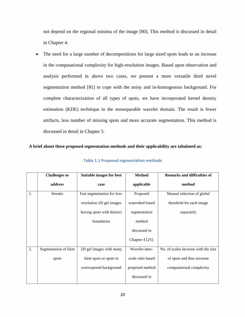
The need for a large number of decompositions for large sized spots leads to an increase
in the computational complexity for high-resolution images. Based upon observation and
analysis performed in above two cases, we present a more versatile third novel
segmentation method [81] to cope with the noisy and in-homogenous background. For
complete characterization of all types of spots, we have incorporated kernel density
estimation (KDE) technique in the nonseparable wavelet domain. The result is fewer
artifacts, less number of missing spots and more accurate segmentation. This method is
discussed in detail in Chapter 5.
A brief about these proposed segmentation methods and their applicability are tabulated as:
Table 1.1 Proposed segmentation methods
Challenges to
address
Suitable images for best
case
Method
applicable
Remarks and difficulties of
method
1. Streaks Fast segmentation for low-
resolution 2D gel images
having spots with distinct
boundaries
Proposed
watershed based
segmentation
method
discussed in
Chapter 4 [25].
Manual selection of global
threshold for each image
separately
2. Segmentation of faint
spots
2D gel images with many
faint spots or spots in
overexposed background
Wavelet inter-
scale ratio based
proposed method
discussed in
No. of scales increase with the size
of spots and thus increase
computational complexity

21
Chapter 4[80].
3 Reduction of artifacts
Segmentation of all
types of spots
Separation of
overlapped spots
Any 2D gel images or any
noisy images containing
several blob objects
Wavelet and
KDE based
proposed method
discussed in
Chapter 5[81].
Performance may be slightly
improved by incorporating
elliptical fitting for separation of
overlapped spots at the cost of
computational complexities

22
Chapter 2 Multi-Scale Processing and Nonseparable Wavelets
2.1 Introduction
The wavelet transform has allowed scientists and engineers to analyze the time varying and
transient phenomena of a signal. The Continuous Wavelet Transform (CWT) is used to measure
the similarity between the signal and the analyzing wavelet function. The CWT represents the
signal in terms of translated and dilated versions of the mother wavelet. The discrete version of
CWT is called Discrete Wavelet Transform (DWT). A dyadic sampling of the time-frequency
plane results in a very efficient algorithm for calculating the DWT. Dyadic Multiresolution
Analysis (MRA) is one of the techniques which help us study how to analyze functions in the
space ℒ2 ℝ at different scales. The different scales at which the functions are analyzed are
powers of 2.
In this chapter, we are going to see how and why wavelets are used in processing data across
scales. The axioms of dyadic MRA are briefly discussed in this chapter. We will discuss
singularities and noise removal. Noise removal is an important pre-processing step for analyzing
any real signal or detecting singularities. We present a brief overview of the different types of
noise present in signals.
An image is a 2D signal, whose intensity is a function of two variables (horizontal, vertical
coordinates). However, images contain multi-dimensional features such as smooth contour and
are not simply stacks of 1D piecewise smooth scan-lines. Discontinuity points (edges) are
typically located along smooth curves/contours due to smooth boundaries of physical objects.
Thus, natural images contain intrinsic geometrical structures that are key features of visual
information. Due to simplicity and low computational complexity, tensor product of 1D wavelet

23
is used to analyze the images. Because of the anisotropic nature and rectangular sampling
support, this formulation captures the singularities in limited directions (horizontal, vertical and
diagonal) only.
The multi-dimensional filter banks are preferred over tensor product of 1D wavelet for better
frequency selection, better extraction of geometrical and directional features of the images. It
involves the mathematical concepts of lattices in the form of sampling. Rectangular sampling
results in a separable wavelet which is the extension of the 1D wavelet. It is not considered as an
efficient way to sample a multi-dimensional band limited signal. A non-rectangular sampling
geometry can represent the band limited signal in efficient way. The nonseparable wavelets using
arbitrary sampling lattices provide the advantage of more degrees of freedom and hence allow
better design of the filter bank adapted to signal geometry.
The wavelets are implemented using filter banks. The lifting framework provides fast
implementation and decomposes the filter banks into a finite sequence of simple filtering steps
known as predict and update steps. The decomposition asymptotically reduces the computational
complexity of the transform.
2.2 Dyadic Multiresolution Analysis (MRA)
In Dyadic MRA, we study how to analyze functions in space ℒ2 ℝ at different scales. In
dyadic MRA, the scale is discretized by powers of two and the time axis is translated by discrete
steps corresponding to the given scale. The basic theory of Dyadic MRA helps in understanding
why wavelets are actually used for processing data across scales. So, a different perspective of
the axioms of dyadic MRA and the theorem of MRA is presented below. To make it easier to
appreciate this, we use Haar MRA as the context of the discussion.

24
2.2.1 Axioms of Dyadic MRA
1. Ladder Axiom: The name Ladder axiom is due to the way subspaces are organized. Let
𝑉0, 𝑉1,… . , 𝑉𝑛 be a ladder of subspaces which belong to ℒ2 ℝ . Each subspace 𝑉𝑖 , 𝑖 ∈ ℤ contains
functions which are piecewise constant in the intervals 2−𝑖𝑙, 2−𝑖 𝑙 + 1 , 𝑙 ∈ ℤ, then
2 1 0 1 2... ...V V V V V
(2.1)
Intuitively, a function which is piecewise constant in the intervals 2−(𝑖+1)𝑙, 2−(𝑖+1) 𝑙 +
1 , 𝑙 ∈ ℤ is also piecewise constant in the intervals 2−𝑖𝑙, 2−𝑖 𝑙 + 1 , 𝑙 ∈ ℤ. To span the entire
subspace 𝑉𝑖 , a set of linearly independent functions which belong to 𝑉𝑖 are used. They are called
the basis functions for 𝑉𝑖 . From the above axiom, we can say that the basis functions of 𝑉𝑖+1 can
be used to represent the functions in 𝑉𝑖 .
As the above axiom is interpreted, it is observed that as a function in a lower subspace is
contracted it becomes a part of the higher subspace and vice versa, as illustrated in the next sub-
section. It implies that the above subspaces are self-similar in nature. Hence, the basis of the
above subspaces is also self-similar. As we see each subspace contains the information of a
signal corresponding to that “scale”. This property of a subspace embedded in another subspace
is exclusively used for analyzing singularities and self-similar functions. Singularity refers to
discontinuity in the signal. This property of singularities propagates through scales. This is
because the information obtained at one scale is embedded in another scale. So, a trend is
observed at the singular points across each scale. By observing this trend we can detect
singularities in the given data. We will discuss singularities in more details in the later sections.
The ladder axiom also brings out the fact that the basis of MRA is self-similar in nature, which,
in turn, helps out in analyzing the self-similar functions effectively.
25
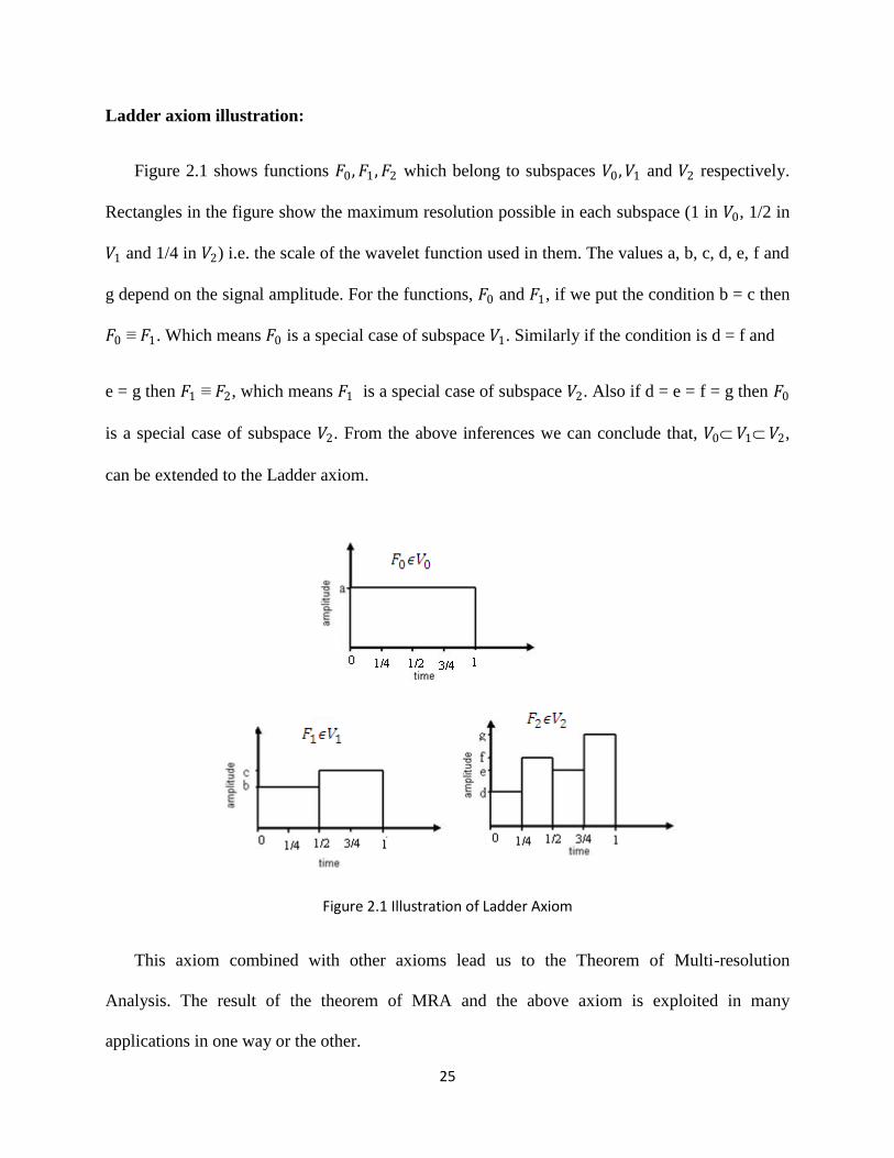
Ladder axiom illustration:
Figure 2.1 shows functions 𝐹0, 𝐹1, 𝐹2 which belong to subspaces 𝑉0,𝑉1 and 𝑉2 respectively.
Rectangles in the figure show the maximum resolution possible in each subspace (1 in 𝑉0, 1/2 in
𝑉1 and 1/4 in 𝑉2) i.e. the scale of the wavelet function used in them. The values a, b, c, d, e, f and
g depend on the signal amplitude. For the functions, 𝐹0 and 𝐹1, if we put the condition b = c then
𝐹0 ≡ 𝐹1. Which means 𝐹0 is a special case of subspace 𝑉1. Similarly if the condition is d = f and
e = g then 𝐹1 ≡ 𝐹2, which means 𝐹1 is a special case of subspace 𝑉2. Also if d = e = f = g then 𝐹0
is a special case of subspace 𝑉2. From the above inferences we can conclude that, 𝑉0 𝑉1 𝑉2,
can be extended to the Ladder axiom.
Figure 2.1 Illustration of Ladder Axiom
This axiom combined with other axioms lead us to the Theorem of Multi-resolution
Analysis. The result of the theorem of MRA and the above axiom is exploited in many
applications in one way or the other.

26
2. Axiom of perfect reconstruction: When a closed union of all the 𝑉𝑖‟s is taken we get
the ℒ2 ℝ space.
𝑉𝑖𝑖∈ℤ
= ℒ2(ℝ)
(2.2)
Intuitively we can say that if we take the union of all the functions which are piecewise
constant at different scales of powers of 2, we can go arbitrarily close to a function in ℒ2(ℝ) .
This axiom reveals that a function in ℒ2(ℝ) can be reconstructed back almost perfectly if the
information across each scale or in each subspace is preserved.
3. The intersection of all the subspaces is the trivial subspace {0}. This is because a function
cannot have a finite energy and be piecewise constant with an infinite support. This axiom also
reveals that a function in ℒ2(ℝ) has significantly less information at scales which have large
support and as the length of the time scale reaches infinity, the content of the signal approaches
zero. The mathematical equation is given in (2.3).
𝑉𝑖 = 0
𝑖𝜖𝑍
(2.3)
4. If a function 𝑥 𝑡 ∈ 𝑉0 ,then 𝑥(2𝑖𝑡) ∈ 𝑉𝑖. Intuitively, we can say that if a function belongs to
𝑉0 , then the time scaled version of the same function belongs to its respective 𝑉𝑖 . This axiom
implies that when a function is contracted or expanded by a factor of 2, the function moves into a
different subspace in the same ladder.
5. Similarly, if 𝑥 𝑡 ∈ 𝑉0 ,then 𝑥 𝑡 − 𝑛 ∈ 𝑉0,𝑛 ∈ ℤ. It can be generalized as, if 𝑥 𝑡 ∈ 𝑉𝑖 then
𝑥 𝑡 − 𝑛2−𝑖 ∈ 𝑉𝑖 , 𝑛 ∈ ℤ, i.e., if a function belongs to 𝑉𝑖 , then the same function translated by a
discrete step also belongs to 𝑉𝑖 .

27
6. Axiom of orthogonal Basis: There exist a function Φ 𝑡 and its integer translates, which form
an orthogonal basis for 𝑉0. Then by using axioms 4 and 5 we can establish the orthogonal basis
for the rest of the 𝑉𝑖‟s i.e., Φ 2𝑖𝑡 and its integer translates form the basis for 𝑉𝑖 . This axiom lays
down the basic foundation in decomposing the signal into different scales.
These subspaces can also be thought of as those subspaces which give some approximate
information of a function at each time scale. So while we move from one subspace 𝑉𝑖 to the next
level of subspace 𝑉𝑖+1,we require some incremental information about the function. The theorem
of Multi-resolution analysis helps us to establish results about this incremental information.
From the above results we can actually bring out a relation between the ladder of subspaces.
From axiom 1 and axiom 6 we can establish the following result:
𝜙 𝑡 = 𝑛 𝜙 2𝑡 − 𝑛 , (𝑛)
𝑛∈ℤ
𝑖𝑠 𝑎 𝑑𝑖𝑠𝑐𝑟𝑒𝑡𝑒 𝑠𝑒𝑞𝑢𝑒𝑛𝑐𝑒 (2.4)
This relation is valid because any function in 𝑉0 can be represented with the basis of 𝑉1. It
can be seen that 𝜙 𝑡 can be expressed as a linear combination of its contracted and translated
versions 𝜙 2𝑡 − 𝑖 , 𝑖𝜖ℤ. This property is exhibited by self-similar functions. Hence, the basis of
these 𝑉𝑖 sub spaces are self-similar. These basis which are self-similar by themselves, are very
useful and efficient in representing self-similar data.
2.2.2 Theorem of MRA
Given the axioms of Multi-resolution analysis, there exists a function 𝜓(𝑡) ∈ ℒ2 ℝ and
𝜓(𝑡) ∈ 𝑉1 such that {𝜓 2𝑚𝑡 − 𝑛 }𝑚∈ℤ,𝑛∈ℤ forms an orthogonal basis for ℒ2(ℝ).
Proof of this theorem can be referred in [26] [82] [83]. The space spanned by {𝜓 2𝑚𝑡 −
𝑛 }𝑚∈ℤ,𝑛∈ℤ is denoted by 𝑊𝑚 . These subspaces can be thought of as incremental subspaces

28
which give incremental information of a function while moving from one scale to another.
While establishing the proof of this theorem we can form several results. We know that,
𝑉𝑖𝑖∈ℤ
= ℒ2(ℝ)
(2.5)
Also,
𝑉𝑚+1 = 𝑉𝑚 ⊕ 𝑊𝑚 (2.6)
Using Equations (2.5) and (2.6) we can form a chain equation resulting in the following
equation.
ℒ2 ℝ = 𝑉0 ⊕ (⊕𝑛=0𝑛=∞ 𝑊𝑛) (2.7)
Using the above result any function 𝑓 𝑡 in ℒ2 ℝ can be represented as follows:
𝑓 𝑡 = 𝑎𝑛𝜙 𝑡 − 𝑛 + 𝑏𝑚 ,𝑛𝜓(2𝑚𝑡 − 𝑛)
∞
𝑚=0
,
∞
𝑛=0
∞
𝑛=0
(2.8)
where,𝑎𝑛 = ∫ 𝑓 𝑡 𝜙(𝑡 − 𝑛)𝑑𝑡
<𝑡>
𝑏𝑚 ,𝑛 = 2𝑚/2 𝑓 𝑡 𝜓 2𝑚 𝑡 − 𝑛 𝑑𝑡
<𝑡>
(2.9)
The representation of the signal as shown in equation (2.9) is called the dyadic wavelet
transform. The coefficients 𝑎𝑛 and 𝑏𝑚 ,𝑛 provide a lot of information about a signal at a
particular scale and at a specific region of time in the frequency band corresponding to that scale.
The spectral content of 𝜙 𝑡 is concentrated around zero frequency whereas that of 𝜓 𝑡 is
concentrated around a non-zero frequency between 0 and 𝜋. So, the functions 𝜙 𝑡 and 𝜓 𝑡 are
approximately Low Pass and Band Pass functions. Particularly, 𝜓 𝑡 at different scales acts as
the impulse response of a band-pass filter of different pass band frequencies. So, if we consider a

29
particular 𝑏𝑚 ,𝑛 it gives information about the signal in the interval 𝑛2−𝑚 , 𝑛 + 1 2−𝑚 and
information about the spectral content in the pass band frequencies of 𝜓(2𝑚 𝑡). So, when a
function is decomposed in the above way, information about that function in a specific region of
time and in a particular frequency band corresponding to the given scale is obtained. This is the
reason why wavelets have become an efficient tool for processing data across scales. This way of
representing data helps in many applications of signal processing including fractals [27] [29].
2.3 Singularities and Noise behavior
2.3.1 Singularities
A singularity is, in general, a point at which the signal blows up or becomes degenerate in
some particular way such as differentiability. Singularities and irregular structures generally
carry the most important information in any signal. In 2D signals such as images, irregular
structures like sharp changes in intensity provide the contour location and help in recognition.
For other signals like electrocardiograms and sound pressure waves, the interesting information
lies in the transients like peaks and troughs, all of which constitute singularities. Also, it is
equally important to study the irregularities in any signal to study its deviation from ideality to
detect several abnormalities. Different types of singularities are shown in Figure 2.2.
Figure 2.2: Types of Singularities

30
Before wavelets became an often used signal processing tool, the Fourier transform was the
sole mathematical tool available to analyze singularities. The Fourier transform indicates the
global overall regularity of a signal but fails to provide the spatial location of the singularity. Due
to this constraint, the Short-Time Fourier Transform (STFT) was introduced, which could
provide the spatial location of the singularities. The STFT could still not provide a good enough
resolution in both time and frequency simultaneously. There had to be a trade-off between time
resolution and frequency resolution. The Wavelet transform was a carefully meditated approach
to deal with these diverse issues [30]. Wavelet transform breaks the signal into several building
blocks, which are well localized in both space and frequency simultaneously.
2.3.2 Wavelets in Singularity Detection
Singularities in a signal without noise
Stephane Mallat and Wen Liang Hwang explained the notion of singularity detection in a
signal by decomposition over a wavelet function, which is the derivative of a zero phase, low
pass smoothing function [31]. They further found that the information in a signal is mainly
represented by the wavelet transform modulus maxima (WTMM) and can be used to locate the
singularities in any signal, whether one-dimensional or two-dimensional. One of the main
features of the wavelet transform is that it retains and, in fact, emphasizes the points of
singularities in the original signal. To locate these singularities, an appropriate threshold can be
applied on the sub-bands. We can get an idea of the WTMM method through the simple example
depicted in Figure 2.3.

31
Figure 2.3: Retention of singularities across the scales
In the above example, singularities are located at (x=30, 60, 90) in the original signal
(without noise). It is visible that from Figure 2.3, the locations of these singularities are retained
across the scales. If we take modulus maxima of the wavelet transform at multiple scales, exact
locations of singularities can be obtained. Now, we will see what happens in signals
contaminated by noise.
Singularities in noisy signals
The main theme of this chapter is to exploit the correlation of wavelet information across
scales. This correlation is very important in terms of removing the noise from the signal. In the
wavelet transform of a noisy signal, the singularities of the original signal and some part of the
noise are retained at each scale. A. Pizurica and her colleagues exploited this interscale
0 10 20 30 40 50 60 70 80 90 100-0.5
0
0.5
1
1.5
x
f(x)
Original Signal
0 10 20 30 40 50 60 70 80 90 100-1
-0.8
-0.6
-0.4
-0.2
0
0.2
0.4
0.6
0.8
1
x
W f
(21,x
)
Wavelet Transform at scale=1
0 10 20 30 40 50 60 70 80 90 100-1
-0.8
-0.6
-0.4
-0.2
0
0.2
0.4
0.6
0.8
1
x
W f
(22,x
)
Wavelet Transform at scale=2

32
information successfully to classify the wavelet coefficients [32]. If a coefficient has a smaller
magnitude at a coarser scale, then its descendants at finer scales are likely to be small.
Conversely, if coefficients corresponding to features are of larger magnitude at a finer scale, its
parents at coarser scale are likely to be large. However, for coefficients caused by noise, the
magnitudes will always decay along the scales, as shown in Figure 2.4. As one can see, the
amplitude of the coefficients corresponding to singularities keeps on increasing from W1 to W3
and those corresponding to noise keeps on decreasing, giving only the signal singularities at
scale 3.
Figure 2.4: Illustration of noise removal using ‘db8’: (a) original signal, (b) signal with additive random
noise, (c) detail coefficients at scale 1, (d) detail coefficients at scale 2 and (e) detail coefficients at scale
3

33
2.4 Nonseparable Wavelet
Wavelet transform is a mathematical tool having a family of basis functions with compact
support. Basis functions are dilation and translation of mother wavelet.
Multi-dimensional sampling is represented by a lattice which can be separable or
nonseparable. The research to date has focused more on separable wavelets and can be
performed along one dimension at a time. Indeed, almost all wavelet image coding algorithms
make use of the separable dyadic 2D discrete wavelet transform (DWT) [33], which applies the
DWT separately to the rows and columns of the image. A 2D discrete time filter is a linear time-
invariant system characterized by the transfer function:
𝐻 𝒛 = [𝒏]𝒛−𝒏
𝒏∈𝑍2
(2.10)
Where h[n] is the impulse response of the filter and 𝐙 = z0
z1 is a complex vector. The frequency
response H (ω) of the filter is given by
𝐻 𝝎 = [𝒏]
𝒏∈𝒛𝟐
𝑒−𝑗𝜔 𝒏 (2.11)
A 2D signal is said to be separable if it can be written as a tensor product of two 1D signals i.e.
𝑥 𝒏 = 𝑥0 𝑛0 . 𝑥1[𝑛1] (2.12)
A 2D filter is said to be separable if its impulse response is a separable 2D signal. Or, in other
words, the transfer function of a 2D separable filter can be written as a product of two 1D
transfer functions i.e.
𝐻 𝒛 = 𝐻0 𝑧0 .𝐻1(𝑧1) (2.13)

34
Only if a 2D filter is separable, can it be implemented as two 1D filters, with each operating
along each dimension. However, this is not true for general nonseparable 2D filters.
The advantage of this algorithm is its simplicity, which is beneficial for implementation.
Separable multi-dimensional (MD) wavelets have a limitation in that their frequency support is
always rectangular shaped. This limitation has been discussed in [34]. Consider a 2D sub-band
coding scheme, where we want to separate the input 2D signal (image) into two sub-bands, a
low-frequency sub-band and a high-frequency sub-band. With separable filter banks, this can be
done by dividing the frequency region , either with respect to the horizontal frequency or with
respect to the vertical frequency, as in Figure 2.5(a) and (b).
Separable wavelets are an extension of 1D bases and are good at capturing singularities in a
localized region. In the case of images, objects usually have smooth boundaries which play an
important role in visualizing and recognizing them. The separable wavelets can capture
singularities in limited directions only and thus, they are not efficient in capturing smoothness
across all possible directions. Therefore, a better representation is evolved in the form of
nonseparable wavelets. It contains all the properties of separable wavelets- e.g. multiresolution,
compact support, critical sampling etc. - along with the property of directionality. Some
nonseparable wavelets, such as quincunx, are isotropic in nature and capture singularities in all
directions. The quincunx wavelet has been discussed in detail in this thesis and is found to
provide better results in comparison with 1D wavelets. For more versatile solutions, smoothness
across different directions can be captured more efficiently using a variety of elongated shaped
directional wavelets. The contourlet transform has incorporated this solution using different
directional filter banks [36]-[41].

35
Figure 2.5: Division of frequency region with 2D two channels separable filter banks, (a) vertical, (b)
horizontal [34]
2.4.1 Building Blocks of Multi-rate System
Similar to filter banks in 1D, 2D filter banks also have two basic building blocks, up-sampler
and down-sampler. These basic operations are best understood using the concept of lattices.
Consider a vector 𝑛 ∈ ℤ2and V is a non-singular 2x2 matrix. Lattice generated by matrix V,
denoted by LAT(V) is the set of all two component vectors x such that x = V n and V is called
generating matrix of LAT(V). Clearly, the cardinality of set LAT(V) is infinity. For discrete time
2D signals, elements of V must be integers. We must note that lattice generated by a matrix V is
unique but the converse is not true. For any unimodular matrix E, LAT (V) = LAT(V E).
For Example, lattice generated by Quincunx matrix Q = 1 11 −1
is shown in Figure 2.6.
Note that the two vectors marked in the figure are the column vectors of the Quincunx matrix.
The lattice points are linear combinations of these columns. It can be seen that the lattice
generated by any matrix is a linear combination of the column vectors of the corresponding
matrix. Also, note that the integer grid ℤ2 can be seen as lattice generated by an identity matrix I,

36
i.e., LAT (I). Both the basic operations up-sampling and down-sampling are described using a
non-singular integer matrix (also called as sampling matrix).
Figure 2.6: Lattice generated by Quincunx matrix
2.4.1.1 Down-Sampling
In simple terms, down-sampler or decimator (characterized by decimation matrix M) accepts
only points which are in the mapping of a point on LAT(M). Mathematically, if y is the
decimated signal and x is the input signal, then 𝑦 𝑛 = 𝑥[𝑀𝑛]. Down-sampling operation is
shown in Figure 2.7 for Quincunx matrix.
Clearly, retained sample locations are linear combinations of the columns of the sampling
matrix M. The columns of the matrix M form a parallelepiped, referred to as the fundamental
parallelepiped FPD(M). In 2D case, FPD(M) is a parallelogram but in higher dimensions, it is a
parallelepiped. FPD(M) = set of all the points Mx, with 𝑥 = [0,1)2. N(M) is the set of integer
vectors in FPD(M). J(M) is the number of integer vectors in FPD(M).
𝐽 𝑀 = det(𝑀) (2.14)

37
Figure 2.7: (a) Before down-sampling, (b) Down-sampling by Quincunx matrix
As the decimator picks only integer points (i.e., from set N(M)), it picks one out of J(M)
points. Hence, the decimation ratio is J(M). To understand the aliasing caused by the decimator,
we need to analyze it in the frequency domain. Fourier transform of the decimator is given by:
𝑌 𝜔 =1
𝐽(𝑀) 𝑋(𝑀−𝑇𝜔 − 2𝜋
𝑘∈𝑀(𝑁𝑇)
𝑀−𝑇𝑘) (2.15)
Output at each frequency ω can be obtained by summing the signal as a set of J(M) aliasing
frequencies 𝑀−𝑇𝜔 − 2𝜋𝑀−𝑇𝑘 where k is a point in N(M). Therefore, there are J(M) - 1 aliases
of the original signal. To get the original signal back, any one of J(M) bands can be non-zero at a
time. Similar to 1D, a decimator simply maps a baseband signal and its J(M)-1 shifted copies,
which are centered at the offset frequencies 2𝑀−𝑇𝑘, to unit frequency cell[−𝜋, 𝜋]2. As an
example for the down-sampling matrix 1 12 −2
, J(M)=4. Therefore, there will be 3 aliased
regions. Figure 2.8(a) shows the baseband frequency support and Figure 2.8(b-d) show three
aliases.
A filter H(z) can be used to remove all but one of the aliases and then decimate the signal to
get the down-sampled signal. The filter H (z) is called decimation filter. The process is shown in

38
Figure 2.9. Superficially it looks like we cannot select the pass band for the decimation filter
arbitrarily and it gets fixed as soon as the matrix and signal are fixed, but a closer look tells us
that we can actually choose the shape of the pass band arbitrarily and yet get the correctly
decimated signal. The only requirement is that one should not have copies of any frequency ω in
any other alias band.
Figure 2.8: (a) Based-band region (b), (c) and (d) three aliases for decimation matrix M

39
Figure 2.9: Decimation
2.4.1.2 Up-Sampling
Up-sampler (characterized by non-singular matrix M) maps a signal on the integer lattice, to
a signal that is non-zero only on the points of the lattice generated by matrix M. Mathematically,
the output is related to the input as follows:
𝑦 𝑛 = 𝑥 𝑀−1𝑛 , 𝑖𝑓 𝑀−1𝑛 ∈ ℤ2
0, 𝑒𝑙𝑠𝑒
(2.16)
Figure 2.10: Up-sampling using matrix M (a) (a) Input signal (b) Up-sampled signal
The process has been shown for matrix 1 12 −2
in Figure 2.10. Figure 2.10 (a) shows the
2x3 input signal and Figure 2.10(b) shows the output signal after up-sampling using the above

40
matrix. In frequency domain, 𝑌 𝑍 = 𝑋(𝑍𝑀). A vector 𝑍 = 𝑍0
𝑍1 raised to matrix power
𝑀 = 𝑀00 𝑀01
𝑀10 𝑀11 is defined as follows: 𝑍𝑚 is a vector whose i
th entry is 𝑍0
𝑀0𝑍1𝑀1 . In Fourier
domain, 𝜔 = 𝑋 𝑀𝑇𝜔 . Therefore, in Fourier domain up-sampling compresses pass-bands and
skews their orientations (simple analogy to 1D case, where pass-band is simply compressed and
scaled). One more feature to note is that the up-sampler gives a mapping such that J(M) similar
compressed pass-bands are mapped to the unit cell. One unit cell of input is mapped to
𝑆𝑃𝐷(𝜋𝑀𝑇) which is defined as the set of all points 𝜋𝑀𝑇𝑥, where 𝑥 ∈ [−1,1)2. An up-sampler
followed by a filter G(z) that passes only one of the compressed images and filters out all others
is known as an interpolator. This is shown in the Figure 2.11. A perfect reconstruction filter bank
is shown in the Figure 2.12. For a detailed derivation, refer to [35].
Figure 2.11: Interpolator
Figure 2.12: Perfect reconstruction filter bank

41
2.5 Quincunx Wavelet Transform
The quincunx is the simplest nonseparable decomposition which can be implemented using
two-band filter bank. Due to the diamond shape support, a low pass filter has a diagonal cut off
which is best suited for the human visual system. The detailed band captures the isotropic
singularity and low pass band produces the approximate image. The quincunx has many
applications in image processing such as denoising, texture characterization and video coding.
The isotropic nature of quincunx filter banks utilizes the smoothness across contour direction
which is needed at each scale for an in-depth study of noisy images [34] [35]. The quincunx has
many applications in image processing such as denoising, texture characterization and video
coding.
The subsampling process generates a sublattice starting from an input lattice. In general, the
subsampling matrix D characterizes the subsampling of a discrete signal X(n) through the
following equation:
𝑌 𝑛 = 𝑋 𝐷𝑛 𝑤𝑖𝑡 𝑛 = (𝑛1, 𝑛2 )𝑇 (2.17)
Y (n) is the signal after subsampling. For example, the dyadic sublattice, which is rectangular, is
determined by:
𝐷𝑑 = 2 00 2
(2.18)
Or equivalently,
𝑌 𝑛1, 𝑛2 = 𝑋(2𝑛1, 2𝑛2) (2.19)
This is the most familiar way of subsampling for the 2D DWT. In this case, the matrix is
diagonal, which implies the separability of dyadic subsampling. Indeed, horizontal and vertical

42
subsampling can be performed separately. The subsampling factor N is given by 𝑁 =
𝐷𝑒𝑡(𝐷) = 4, implying that the number of samples per channel is reduced by the factor 4.
Consequently, the wavelet filter bank has 4 channels with filters corresponding to three wavelets
and one scaling function. Furthermore, the scaling factor is given by 𝑆 = 𝑁 = 2. Hence, for
dyadic subsampling the horizontal and vertical dimensions are reduced by the factor 2. The
Quincunx lattice is shown in Figure 2.13, where gray dots represent the points on the Quincunx
lattice.
Analogously, the following matrix characterizes the non-rectangular quincunx sublattice:
𝐷𝑞 = 1 11 −1
(2.20)
Or equivalently,
𝑌 𝑛1,𝑛2 = 𝑋(𝑛1 + 𝑛2, 𝑛1 − 𝑛2) (2.21)
In this case, the quincunx sublattice is nonseparable because the matrix is not diagonal.
Furthermore the subsampling factor N equals 2, which implies that the quincunx 2D DWT has
two channels corresponding to one wavelet and one scaling function. This is similar to the 1D
DWT. In each channel the number of samples is reduced by the factor 2 and the horizontal and
the vertical dimensions are reduced by the scaling factor 2 .
If we iterate the filter bank to obtain higher level decompositions, then the new sublattice is
characterized by a matrix which is an integer power of the subsampling matrix D. For example,
after two iterations or equivalently two decomposition levels, equation (2.21) becomes
𝑌 𝑛1, 𝑛2 = 𝑋(2𝑛1, 2𝑛2). It is same as equation (2.18) which is a separable lattice, so we obtain
for the quincunx case the following subsampling matrix:

43
𝐷𝑑 = 2 00 2
(2.22)
In general, the quincunx sublattice obtained after an even number of iterations corresponds
to the dyadic sublattice with half the number of iterations. In quincunx, an odd number of
iterations correspond to the nonseparable lattice and an even number of iterations corresponds to
the separable lattice. Therefore, the quincunx 2D DWT requires twice the number of
decomposition levels of the dyadic 2D DWT to obtain the same scale reduction factor S.
(0,0)0n
1n
Figure 2.13: The Quincunx lattice (shaded point shows lattice points)
The 2-channel Quincunx filter bank is shown in Figure 2.14. The Quincunx low pass and
high pass filters are often chosen to have diamond-shaped frequency supports, as shown in
Figure 2.15. With this diamond-shaped frequency response, the low pass filter can preserve the
high frequencies in the vertical and horizontal directions, which is a good match to the human
visual system since the visual sensitivity is higher to changes in these two directions than the
other directions.

44
Figure 2.14: Quincunx filter bank
Figure 2.15: Frequency supports of filters in Quincunx filter bank
2.6 Lifting Scheme
Lifting scheme is a method developed by Wim Sweldens [70] for the construction of
biorthogonal wavelets without using the Fourier transform. It requires far fewer computations
and reduced memory for the DWT. The main motivation behind the development of the lifting
scheme and the several related ideas was the search for fast algorithms to compute compact
representations of functions and data sets using wavelets and filter banks.
Lifting consists of three stages, which are referred as split, predict, and update. These three
stages will be briefly explained below. Consider a signal 𝑐𝑗 with 2𝑗 samples which we want to
transform into a coarser signal 𝑐𝑗−1 and detail 𝑑𝑗−1.
ω1
ω0
H0
π,- π
π,π -π, π
-π,- π
ω1
ω0
H1
-π, π π,π
-π,- π π,- π
X Y
H0(Z) G0(Z)
H1(Z) G1(Z) Q
Q
Q
Q

45
Split: In this stage, the signal is split into two disjoint sets of samples. We can form one subset
with even-indexed samples 𝑐2𝑙 and other subsets consisting of the odd indexed samples 𝑐2𝑙+1.
Each subset contains half as many samples as the original signal. The splitting into even and odd
indexed samples is called the lazy wavelet transform.
)(:),( 11
j
jj csplitoddeven
Predict: If the signal has local correlation then we can use the even set to predict the odd one.
Let us define an operator 𝑃(𝑒𝑣𝑒𝑛𝑗−1) for the prediction of the odd set. We then let the detail
𝑑𝑗−1 be the difference between the odd sample and its prediction.
)( 11
1
jj
j evenPoddd
In the case of Haar, the prediction is particularly simple.
j
l
j
l
j
l ccd 212
1
Update: One of the key properties of the coarser signal is that it has the same average value as
the original signal. It defines an operator Up of the form
)( 1
1
1
j
j
j dUpevenc
All this can be computed in place: The even location can be overwritten with the averages
and the odd ones with details. An abstract implementation is given by
);(:),( 11 jjj csplitevenodd
);(: 11 jj evenPodd

46
);(: 11 jj oddUeven
The lifting structure guarantees Perfect Reconstruction (PR), and the so-called predict and
update lifting steps can be used to increase the order of the polyphase matrix (and thus of the
filters) while maintaining PR. Predict and update steps involve factorizing the analysis polyphase
matrix in factors of the following form:
𝐸′ 𝑧 = 𝐻𝑒 𝐻𝑜
𝐺𝑒 𝐺𝑜
= 1 𝑈(𝑧)0 1
1 0
−𝑃(𝑧) 1
(2.23)
The corresponding synthesis matrix is given by
𝑅′ 𝑧 = 𝐻𝑒 𝐻𝑜
𝐺𝑒 𝐺𝑜 =
1 0𝑃(𝑧) 1
1 −𝑈(𝑧)0 1
(2.24)
Where 𝐻 and 𝐺 are the analysis filter banks and H and G are the synthesis filter banks.
Lifting scheme is PR by construction, regardless of the specific choice of the update 𝑈 𝑧 or
predicts 𝑃(𝑧) steps.
By using multiple such update and predict steps, with different 𝑃(𝑧) and 𝑈(𝑧) functions, a
Quincunx filter bank with higher order filters can be constructed. The lifting framework is shown
in Figure 2.16.
(a) Analysis

47
(b) Synthesis
Figure 2.16: Lifting Structure for Quincunx filter Bank in (a)-Analysis and (b)-Synthesis. The symbols
‘A’,’A1’,’D1’ and ’Ȃ’ represent input signal, approximation signal at next scale, detail signal at next scale
and reconstructed signal respectively. The symbols ‘P4’ and ‘U4’ represent fourth order predict and
update filters respectively.

48
Chapter 3 Denoising Of 2DGE Images
3.1 Introduction
The undesirable components of an image are termed as noise. The presence of noise in
2DGE images might lead to false detection and classification, which might reduce the accuracy
of a computer aided diagnostic system. Hence, denoising is a vital part of dealing with 2D Gel
images. Generally, the noises that affect images can be classified into additive and multiplicative.
Additive noise includes Gaussian noise, salt & pepper noise and uniform noise. Multiplicative
noise, such as non-isometric noise and shot noise, is a by-product of the stochastic nature of the
image acquisition system. Additive noise is independent of the spatial and spectral distribution of
the image, while, multiplicative noise is dependent on the image and is difficult to remove
without impairing the image. Since the noise variation greatly depends on the intensity levels of
the image pixels being corrupted, it is not easy to establish an appropriate statistical model for
the noise simply by examining the corrupted image.
The nonlinearities in the gel formation and image acquisition process lead to distortions,
overlapped protein spots, saturated spots, faint spots, non-linear intensity and uneven background
in the gel images. As a result, pre-processing steps are important before image analysis.
Denoising is one of the most important pre-processing steps, and the overall accuracy of protein
spot detection and analysis depends crucially on how effectively the gel images have been
denoised.
Since denoising is the first operation in pre-processing operations pipeline, if successful, it
may greatly impact results of downstream steps in the following ways:

49
It prevents over-estimation of the image background and helps extracting faint, yet
significant, spots [42].
It prevents the formation of misleading spots (artifacts), thus resulting in more truthful
spot matching and more accurate determination of the significant spots which have to be
further analyzed by mass spectrometry methods.
It leads to a more accurate estimation of spot properties (e.g. spot volume) leading to an
improved spot differential analysis which is key for reliable biomarkers identification
[43].
In the image denoising process, a trade-off must be made between noise suppression and
preservation of singularities in the image. In case of 2DGE images, we expect the denoising
process to remove the following features without introducing any significant distortions in an
image:
Background unevenness
High-frequency noise
Salt and pepper noise introduced due to dust
Horizontal and vertical streaks
In this chapter, we have compared the different available methods of denoising in order to
find the one which suits best for the 2D gel electrophoresis images. We proposed the use of
nonseparable wavelet in denoising methods.
3.2 Denoising Techniques
Denoising techniques, in general, are quite mature and have attracted a lot of research. Noise
is inherent in all image acquisition systems and needs to be removed for accurate analysis of

50
images. A thorough literature survey [44] shows currently available techniques for denoising
images.
We have focused on wavelet domain denoising techniques. Most wavelet techniques exploit
the close relationship between denoising and compression. Non-linear thresholding on wavelet
coefficients is a standard way of denoising natural images. This technique is described in detail
in the following section.
3.3 Wavelet Shrinkage Method
Wavelet denoising must not be confused with smoothing; smoothing only removes the high
frequencies and retains the lower ones. Wavelet shrinkage is a non-linear process and this is what
distinguishes it from linear denoising techniques such as least squares. Wavelets are a very
powerful tool for de-correlation and hence, compression. This property makes wavelets a
suitable choice for denoising techniques.
3.3.1 Motivation for Wavelet Shrinkage
As shown in Figure 3.1(a) a signal with singularities is taken and corrupted by additive white
Gaussian noise (AWGN) of SNR 20dB and is then decomposed with the `db6' wavelet. A
histogram of the magnitude of coefficients is shown in Figure 3.1(b). A few important
conclusions can be drawn from the histogram, most of the coefficients are very small, or in other
words, most significant information is represented by a very small number of coefficients (the
tail of histogram). This sparse nature of wavelet coefficients suggests that even if we remove
most of the small coefficients (by making them zero) below a certain threshold and take the
inverse wavelet transform, then the reconstructed signal will retain most of the information and
hence will be noise free.

51
To state more precisely, we are motivated to study this idea of wavelet coefficient shrinkage
based on the following assumptions [45]:
The de-correlating property of wavelet transform creates a sparse signal, i.e. most of the
coefficients are very small (zero or close to zero).
Noise is spread out equally along all coefficients.
The noise level is not too high; hence we can distinguish the signal wavelet coefficients
from the noisy ones.
As it turns out, this method is indeed effective and thresholding is a simple and efficient
method for noise reduction. Further, inserting zeros creates more sparsity in the wavelet domain
and here we see a link between wavelet denoising and compression which has been described in
many sources such as [48].
Figure 3.1: (a) Original signal with singularities (in black) and noisy signal (in yellow)
(b) histogram of magnitude of `db6' wavelet coefficients of noisy signal

52
3.3.2 Thresholding: Soft and Hard
As the name itself suggests, hard thresholding is `keep or kill' procedure. If the magnitude of
a wavelet coefficient is above a certain threshold λ, then keep the coefficient as it is. Otherwise,
kill the coefficient by making it zero. Hard thresholding operator is defined as:
𝐷 𝑈, 𝜆 = 𝑈, 𝑖𝑓|𝑈| > 𝜆
0, 𝑒𝑙𝑠𝑒
(3.1)
It is very simple and intuitive but has some problems associated with it. Sometimes noisy
coefficients may pass through hard thresholding procedure and give unwanted artifacts in the
denoised data. The answer to this problem is soft thresholding.
Soft thresholding operator is defined as:
𝐷 𝑈, 𝜆 = 𝑠𝑔𝑛 𝑈 𝑚𝑎𝑥( 𝑈 − 𝜆, 0) (3.2)
Transfer functions for Hard and soft thresholding are shown in Figure 4.2(a) and (b)
respectively. Contrary to hard thresholding, soft thresholding shrinks the coefficients above the
threshold in absolute value by the same threshold. Soft thresholding has some advantages. It
makes some algorithms mathematically more tractable [49].
Figure 3.2: (a) Hard thresholding (b) Soft thresholding

53
3.3.3 Image Denoising Algorithm
The algorithm for image denoising using wavelet shrinkage is very simple and involves the
following steps:
Calculate the wavelet transform of the image
Threshold the wavelet coefficients
Compute the inverse wavelet transform to get the denoised image
3.3.4 Threshold Determination
It is very important to choose the threshold wisely for proper denoising. If we choose a very
small threshold, we will get an output very close to the input image but it will still be noisy. On
the other hand, if we choose a very large threshold, most of the wavelet coefficients will become
zero, which might result in the killing of some significant image coefficients. This results in a
smoothened image and leads to image distortion. Paying too much attention to smoothness will
lead to a blurred image. In literature, there are various shrinkage methods to determine
thresholds. We will investigate three of them, viz. VisuShrink, SUREshrink, BayesShrink.
3.3.4.1 VisuShrink
VisuShrink is a thresholding technique which applies the universal threshold proposed by
Donoho and Johnstone [46]. This threshold is given by 𝜍 2𝑙𝑜𝑔𝑀 where M is the number of
pixels in the image and σ is the noise variance estimated from the wavelet coefficients of
diagonal details at the first level of decomposition by equation (3.3):

54
𝜍 = 1
. 6745 𝑚𝑒𝑑𝑖𝑎𝑛( 𝐶𝐻𝐻1 )
(3.3)
It is proved [47] that the maximum of any M independent and identically distributed (iid)
values distributed as N (0, σ2) will be smaller than the universal threshold with high probability,
with the probability approaching 1 as M increases. Thus, with high probability, a pure noise
signal is estimated as being identically zero. However, for denoising images, VisuShrink is found
to yield an overly smoothed estimate. This is because the universal threshold is derived under the
constraint that with high probability the estimate should be at least as smooth as the signal. So,
the universal threshold tends to be high for large values of M, killing many signal coefficients
along with the noise. Thus, the threshold does not adapt well to discontinuities in the signal.
3.3.4.2 SUREshrink
Let {𝜇 = 𝜇𝑖 , 𝑖 = 1, …………… . 𝑑} be a d-dimensional vector, and let 𝑥 = 𝑥𝑖 (with 𝑥𝑖
distributed as 𝑁(𝜇𝑖 , 1) be multivariate normal observations with mean vector 𝜇𝑖 . Let 𝜇 = 𝜇 (𝑥)
be a fixed estimate of 𝜇 based on the observations x. SURE (Stein's unbiased Risk Estimator)
[46] is a method for estimating the coefficients by minimizing the loss μ − 𝜇 2 in an unbiased
fashion.
In our case 𝜇 is the soft threshold estimator 𝜇𝑖 (𝑡) = 𝜂𝑡(𝑋𝑖). We apply Stein's result to get an
unbiased estimate of the risk 𝔼 μt(x) − 𝜇 2:
𝑆𝑈𝑅𝐸 𝑡; 𝑥 = 𝑑 − 2. ⋕ 𝑖: |𝑥𝑖 < 𝑡| + 𝑚𝑖𝑛(𝑥𝑖
𝑑
𝑖=1
, 𝑡)2
(3.4)
For an observed vector 𝑥 (in our problem, 𝑥 is the set of noisy wavelet coefficients in a sub-
band), we want to find the threshold T that minimizes 𝑆𝑈𝑅𝐸 𝑡; 𝑥 i.e.

55
𝑇 = argt
min 𝑆𝑈𝑅𝐸(𝑡; 𝑥) (3.5)
3.3.4.3 BayesShrink
In BayesShrink [47], we determine the threshold for each sub-band assuming a Generalized
Gaussian Distribution (GGD). It is a data dependent and sub-band adaptive threshold. Equations
to calculate Bayesian threshold are given as follows:
𝜍 =𝑚𝑒𝑑𝑖𝑎𝑛( 𝑌𝑖𝑗 )
. 6745, 𝑌𝑖𝑗 ∈ 𝑆𝑢𝑏𝑏𝑎𝑛𝑑 𝐻𝐻1
(3.6)
This is an adaptive thresholding procedure, so we need to calculate the threshold for every
detail sub-band separately.
𝑇 =𝜍2
𝜍𝑠
(3.7)
where, 𝜍𝑠 is calculated for each sub-band as given in equation (3.8).
𝜍𝑠 = 𝑚𝑎𝑥 1
𝑛 𝐶𝑖𝑗
2
𝑛
𝑖 ,𝑗=1
− 𝜍2 , 0
(3.8)
Where 𝐶𝑖𝑗 are wavelet coefficients of the sub-band under consideration.
To demonstrate the working of this algorithm, an example is shown in Figure 3.3. Original
image `Lena' was taken and Gaussian noise with standard deviation 0.005 was added to it.
Various shrinkage procedures were applied to the noisy image and the corresponding denoised
images are shown in Figure 3.3. We have obtained good results with Bayes threshold.

56
Figure 3.3: (a) Original Image (b) Corrupted by Gaussian noise (c) Denoised by VisuShrink (d)
Denoised by SUREshrink (e) Denoised by BayesShrink
3.4 Image Denoising: A Wavelet Domain Modeling Approach
In the previous section, we discussed a non-parametric approach to denoise 2DGE images.
In this section, we will discuss a denoising approach based on stochastic modelling of wavelet
coefficients.
Accurate image modelling is a critical component of many image processing tasks. In [48], a
simple yet effective, statistical and spatially adaptive wavelet image model was developed,
which formed the basis of the state-of-the-art estimation quantization (EQ) compression
algorithm. In [49], a closely related model for image wavelet coefficients has been developed
and applied for denoising the images corrupted by additive white Gaussian noise (AWGN). In

57
this dissertation, we have first shown that 2DGE images fulfill the requirements for this model to
be valid and then implemented this model in MATLAB using Quincunx wavelet.
There is a close relationship between image compression and image denoising. In fact, the
use of lossy data compression itself was proposed for denoising with the intuition that a typically
correlated signal is compressible but noise is not [50]. Using this model, this intimate relation
between compression and denoising is exploited using state-of-the-art models for compression.
This model significantly reduces the computational burden yet produces comparable results in
terms of mean-squared error (MSE) and perceptual image quality. The key ingredient of the
algorithm is the use of simple but efficient spatial adaptation techniques. This algorithm is based
on DWT. The transform coefficients within sub-bands are modelled as independent identically
distributed random variables with generalized Gaussian distribution (GGD).
This model takes an approach which exploits the local structure of the wavelet image
coefficients. Also, it uses linear Minimum Mean Squared Error (MMSE) like estimation instead
of coefficient thresholding.
3.4.1 Stochastic Model for Wavelet Coefficient
Image wavelet coefficients are modelled as a realization of a doubly stochastic process.
Specifically, the wavelet coefficients are assumed to be conditionally independent zero-mean
Gaussian random variables, given their variances. These variances are modelled as identically
distributed, highly correlated random variables. A stochastic prior is put on local variances. For
estimation purposes, we approximate wavelet coefficients as locally i.i.d [49]. To verify the
above stated model in 2D gel image as shown in Figure 3.5, we have taken the histogram of the
original high band coefficients from the first scale, obtained by employing Daubechies-8

58
wavelets as shown in Figure 3.4(a). Figure 3.4(b) shows those coefficients normalized by their
estimated standard deviations. Observe that the normalized histogram is well approximated by a
zero-mean, unit variance Gaussian probability density function (p.d.f.).
It is assumed that image pixels are corrupted by AWGN of known variance. Let X(k)
represent the orthonormal wavelet coefficients of the clean image. The wavelet coefficients of
the noisy image are given by Y(k) = X(k) + n(k), where n(k) is AWGN due to orthonormality of
the chosen wavelet transform. The denoising algorithm operates in two steps. Initially, we
perform an approximate maximum a posterior (MAP) estimation of the variance σ2(k) for each
coefficient using the observed noisy data in a local neighbourhood and a prior model for σ2(k).
The estimate 𝜍 2(𝑘) is then substituted for σ2(k) in the expression for the Minimum Mean
Squared Error (MMSE) estimator of X(k). Both these steps are summarized in Figure 3.6(a) and
described in more detail in further sections.
(a) (b)
Figure 3.4: (a) Histogram of the high-band wavelet coefficients of gel Image (b) Blue line: histogram of
the same coefficients scaled by estimated local standard deviations. Red line: unit-variance,
zero-mean Gaussian pdf.

59
Figure 3.5: A 2DGE image from database [1]
3.4.1.1 Denoising Algorithm
Given σ2 (k), the wavelet coefficients X (k) are independent Gaussian variables, so the
MMSE estimator for X (k) is given by:
𝑋 𝑘 =𝜍2 𝑘
𝜍2 𝑘 + 𝜍𝑛2𝑌(𝑘)
(3.9)
We emphasize that this assumes σ 2(k) is deterministic and known. But in fact, σ
2(k) is not
known, so we construct a linear MMSE-like estimator.
𝑋 𝑘 =𝜍 2 𝑘
𝜍 2 𝑘 + 𝜍𝑛2𝑌(𝑘)
(3.10)
where 𝜍 2 𝑘 is an estimate for σ 2(k). Results indicate that performance of the proposed
approximate MMSE predictor is dependent, to a very large extent, on the quality of the estimator
of 𝜍 2 𝑘 .

60
Figure 3.6:(a) Block diagram of the denoising algorithm (b) Histogram of the estimated local variance of
the coefficients (solid line) in wavelet image sub-band, approximated using a single exponential prior
(dash-dotted line) and a mixture of exponentials that consists of three single exponentials in three non-
overlapping regions (dashed line).

61
3.4.1.2 Estimation of Variance Field
The estimation of the variance field σ 2(k) is the crux of this denoising algorithm. For each
data point Y (k), an estimate of σ 2(k) is formed based on a local neighbourhood N (k). We use a
square window N (k) centered at Y (k). Assuming the correlation between variances of
neighbouring coefficients is high, we have σ 2(j) ≈ σ
2(k) for all j € N (k). Then we compute an
approximate Maximum Likelihood (ML) estimator.
𝜍 2 𝑘 = 𝑎𝑟𝑔𝑚𝑎𝑥𝜍2≥0∏𝑗∈𝑁(𝑘)𝑃 𝑌 𝑗 𝜍2 = 𝑚𝑎𝑥 0,1
𝑀 𝑌2
𝑗 ∈𝑁 𝑘 𝑗 − 𝜍𝑛
2 (3.11)
where P(.|σ2|) is the Gaussian distribution with zero mean and variance 𝜍2 + 𝜍𝑛
2 and M is the
number of coefficients in the neighbourhood N(k). Now, assume a prior marginal distribution
𝑓𝜍(𝜍2). Then we obtain an approximate estimate of σ 2(k) as
𝜍 2(𝑘) = 𝑎𝑟𝑔𝑚𝑎𝑥𝜍2≥0∏𝑗 ∈𝑁(𝑘)𝑃 𝑌 𝑗 𝜍2 𝑓𝜍(𝜍2) (3.12)
In Figure 3.6(b), we plot a histogram of the estimated local variances using equation (3.11) with
a 7 x 7 window for a typical high pass sub band of an image (solid line). The exponential prior
𝑓𝜍 𝜍2 = λe−λσ2
(3.13)
shown by the dash-dotted line in Figure 3.6(b) is a reasonable candidate to fit the original
histogram. The approximate MAP estimate for using an exponential prior is given by:
𝜍 2 𝑘 = 𝑚𝑎𝑥 0,𝑀
4𝜆 −1 + 1 +
8𝜆
𝑀2 𝑌2(𝑗)
𝑗∈𝑁(𝑘) − 𝜍𝑛
2
(3.14)
The authors of [49] verified that MAP estimate gives an improvement in denoising
performance over ML estimate. They also experimentally found out that accurate modelling of

62
the histogram does not give any significant improvement as far as denoising is concerned. In this
thesis, we have implemented both ML and MAP estimates and compared them.
3.5 Use of Nonseparable Wavelet
We have implemented the wavelet shrinkage and stochastic methods in nonseparable
quincunx wavelet domain and studied the results. We must note that quincunx wavelet transform
has not been used previously for denoising of gel images. To verify whether we can apply the
stochastic model to 2DGE images using Quincunx wavelets, we decomposed various 8-bit
2DGE images using Quincunx wavelets. We found that all sub-bands are approximately
Gaussian with zero means. In Figure 3.7 (a), (b), (c) and (d), histograms of its various sub-bands
are shown. It can be clearly seen that they are all approximately Gaussian. This is also a good
reason for applying Bayes‟s threshold based wavelet shrinkage method.
3.6 Evaluation Methodology
We have evaluated the performance of all the denoising algorithms described in sections 3.3
and 3.4 using 8-bit synthetic as well as real 2DGE images. We have generated a synthetic gel
image using real 2DGE images by cutting out protein spots from them. We have tried to get all
kinds of spots from real image: saturated spots, streaks, faint spots, overlapping spots etc. We put
these spots on a white background using image editing tools. Further, we added white Gaussian
noise of different variances: 30, 35 and 40 as well as salt and pepper noise. From now on, these
will be referred to as clean image, noisy image-1 (σ = 30), noisy image-2 (σ = 35) and noisy
image-3 (σ = 40). These images are shown in Figure 3.8.
We have applied the denoising procedures on the noisy images and then calculated Peak
Signal to Noise Ratio (PSNR) between denoised image and clean image. Higher the PSNR,

63
better the performance but this is not the only criteria which should be looked at. Since 2DGE
images contain non-stationary noise and non-linear artifacts, only PSNR does not suffice. We
have also looked into artifacts introduced by the denoising procedure. Lower artifacts imply
better performance. Lastly, we compared the performance of various methods with that of the
commercial software Delta2D.
Figure 3.7: Histograms of Quincunx wavelet coefficients of various sub-bands of the 2DGE image in
Figure 3.5. (a) Level-1 Scale-1 (b) Level-1 Scale-2 (c) level-2 Scale-1(d) Level-2 Scale-2
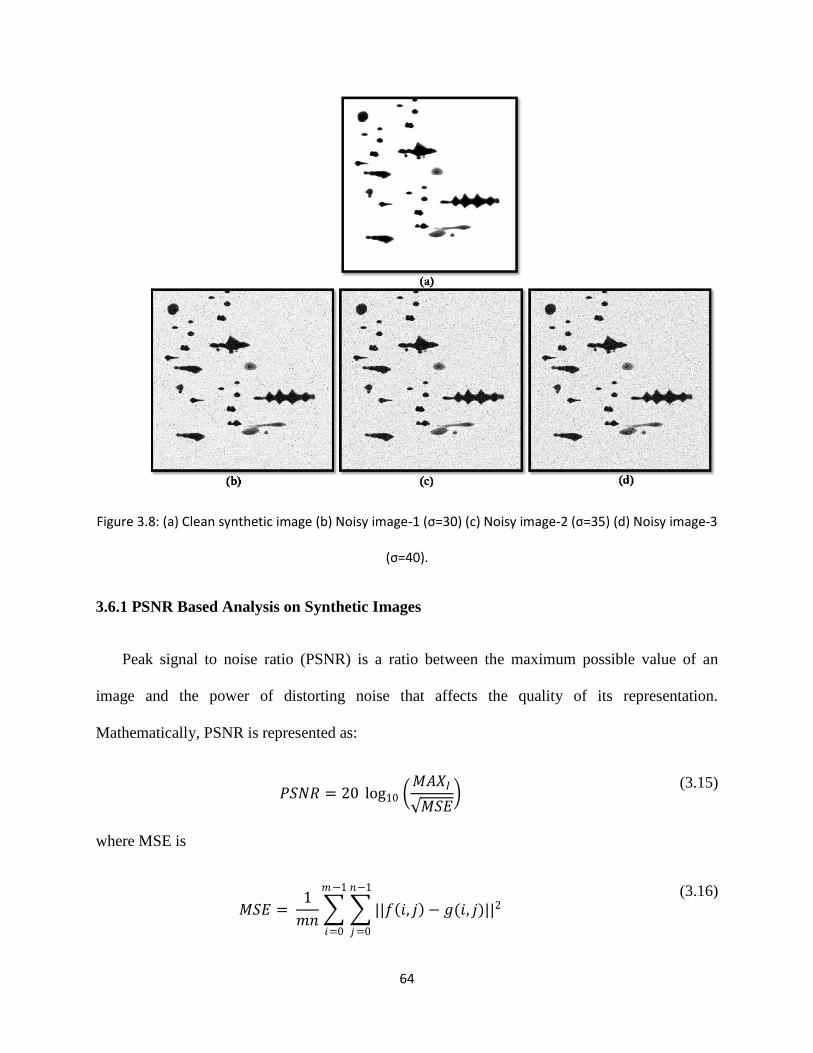
64
Figure 3.8: (a) Clean synthetic image (b) Noisy image-1 (σ=30) (c) Noisy image-2 (σ=35) (d) Noisy image-3
(σ=40).
3.6.1 PSNR Based Analysis on Synthetic Images
Peak signal to noise ratio (PSNR) is a ratio between the maximum possible value of an
image and the power of distorting noise that affects the quality of its representation.
Mathematically, PSNR is represented as:
𝑃𝑆𝑁𝑅 = 20 log10 𝑀𝐴𝑋𝐼
𝑀𝑆𝐸
(3.15)
where MSE is
𝑀𝑆𝐸 = 1
𝑚𝑛 ||𝑓 𝑖, 𝑗 − 𝑔(𝑖, 𝑗)||2
𝑛−1
𝑗=0
𝑚−1
𝑖=0
(3.16)

65
where f is the original image, g is the noisy image and m, n are rows and columns of the image
respectively. 𝑀𝐴𝑋𝐼 is the maximum signal value of the original image.
On synthetic images we added Gaussian noise of σ = 30, 35, 40 and salt & pepper noise.
Denoising was performed using wavelet and known methods; the PSNR of denoised images w.r.t
the original image was obtained for each method. Results are tabulated in Table 3.1-3.3. We
observed that soft thresholding gives better performance than hard thresholding in all cases, as
expected. Bayes threshold gives the best performance among all thresholds. In the Table 3.4,
results are reported for Bayes threshold except for CWT for which bivariate shrinkage has been
used as proposed in [50]. Denoised images for σ = 30 are shown in Figure 3.9.
The PSNR values obtained from undecimated quincunx wavelet transform are better than the
other methods. However, even though the PSNR values of the statistical modelling method are
not high, the images obtained from them seem to be comparable to that of the complex wavelet
transform. Hence, we have selected Quincunx wavelet transform, CWT and statistical modelling
of Quincunx coefficients using MAP rule for the experiments.
The 3D view of original, noisy and denoised images are presented in Figure 3.10. The 3D
view shows that the quincunx denoised image preserves more sharp features as compared to the
coiflet denoised image while providing higher PSNR value [24]. Figure 3.11 presents the
segmented results of the original gel image after denoising. This analysis shows that an image
denoised with quincunx preserves more spots and sharp features and also provides high PSNR
values.

66
Table 3.1 Mean PSNR values for our set of synthetic images with noise variance 40
Wavelet family
PSNR values
Noisy
(𝝈 = 𝟒𝟎) UniU-SoftS UniU-HardH BayesB-SoftS BayesB-HardH
Haar 19.13 19.201 19.137 19.508 19.175
db1D 19.13 19.201 19.137 19.508 19.175
db2 D 19.13 19.218 19.139 19.616 19.195
db3 D 19.13 19.225 19.139 19.696 19.196
db4 D 19.13 19.223 19.138 19.685 19.198
db5 D 19.13 19.22 19.139 19.66 19.223
db6 D 19.13 19.226 19.138 19.684 19.202
db7 D 19.13 19.231 19.138 19.739 19.202
db8 D 19.13 19.228 19.139 19.742 19.2
db9 D 19.13 19.23 19.138 19.743 19.218
db10 D 19.13 19.228 19.139 19.721 19.202
db11 D 19.13 19.225 19.138 19.701 19.19
db12 D 19.13 19.228 19.14 19.744 19.211
db13 D 19.13 19.225 19.138 19.687 19.196
db14 D 19.13 19.232 19.139 19.786 19.203
db15 D 19.13 19.229 19.141 19.764 19.204
coif1 C 19.13 19.228 19.142 19.707 19.211
coif2 C 19.13 19.225 19.14 19.686 19.209
coif3 C 19.13 19.23 19.138 19.75 19.207
coif4 C 19.13 19.228 19.139 19.731 19.202
coif5 C 19.13 19.23 19.138 19.745 19.201
undeci UN-coif 19.13 18.92 19.13 24.726 21.726
quincunx 19.13 19.203 19.139 24.497 21.215
undeci UN-qunicunx 19.13 19.29 19.145 24.498 22
D refers to Daubachies wavelet family,
C refers to coiflet wavelet family,
UN refers to undecimated.
U refers to Universal threshold,
H refers to hard thresholding,
S refers to soft thresholding and
B refers to Bayes threshold.

67
Table 3.2 Mean PSNR values for our set of synthetic images with noise variance 35
Wavelet family
PSNR values
Noisy
(𝝈 = 𝟑𝟓) UniU-SoftS UniU-HardH BayesB-SoftS BayesB-HardH
haar 18.215 18.293 18.224 18.669 18.276
db1D 18.215 18.293 18.224 18.669 18.276
db2 D 18.215 18.306 18.228 18.723 18.288
db3 D 18.215 18.309 18.226 18.78 18.285
db4 D 18.215 18.314 18.225 18.826 18.303
db5 D 18.215 18.313 18.227 18.795 18.29
db6 D 18.215 18.315 18.227 18.842 18.292
db7 D 18.215 18.314 18.224 18.812 18.289
db8 D 18.215 18.313 18.224 18.804 18.289
db9 D 18.215 18.315 18.225 18.839 18.294
db10 D 18.215 18.317 18.225 18.809 18.296
db11 D 18.215 18.317 18.226 18.863 18.305
db12 D 18.215 18.315 18.226 18.832 18.296
db13 D 18.215 18.318 18.224 18.877 18.301
db14 D 18.215 18.312 18.226 18.804 18.293
db15 D 18.215 18.317 18.225 18.856 18.329
coif1 C 18.215 18.312 18.224 18.799 18.288
coif2 C 18.215 18.312 18.225 18.794 18.286
coif3 C 18.215 18.322 18.228 18.912 18.315
coif4 C 18.215 18.314 18.226 18.825 18.297
coif5 C 18.215 18.319 18.224 18.844 18.3
undeci U-coif 18.215 18.036 18.215 24.259 24.259
quincunx 18.215 18.042 18.217 25.994 25.994
undeci U-qunicunx 18.215 18.132 18.215 25.996 25.994
D refers to Daubachies wavelet family,
C refers to coiflet wavelet family,
UN refers to undecimated.
U refers to Universal threshold,
H refers to hard thresholding,
S refers to soft thresholding and
B refers to Bayes threshold.

68
Table 3.3 Mean PSNR values for our set of synthetic images with noise variance 30
Wavelet family
PSNR values
Noisy
(𝝈 = 𝟑𝟎) UniU-SoftS UniU-HardH BayesB-SoftS BayesB-HardH
haar 19.089 19.087 19.089 19.09 19.089
db1D 19.089 19.087 19.089 19.09 19.089
db2 D 19.089 19.09 19.089 19.089 19.089
db3 D 19.089 19.088 19.089 19.092 19.089
db4 D 19.089 19.088 19.089 19.09 19.089
db5 D 19.089 19.089 19.089 19.089 19.089
db6 D 19.089 19.088 19.089 19.09 19.089
db7 D 19.089 19.088 19.089 19.09 19.089
db8 D 19.089 19.089 19.089 19.089 19.089
db9 D 19.089 19.088 19.089 19.09 19.089
db10 D 19.089 19.088 19.089 19.091 19.089
db11 D 19.089 19.088 19.089 19.091 19.089
db12 D 19.089 19.09 19.089 19.089 19.089
db13 D 19.089 19.093 19.089 19.09 19.089
db14 D 19.089 19.089 19.089 19.089 19.089
db15 D 19.089 19.088 19.089 19.09 19.089
coif1 C 19.089 19.088 19.089 19.09 19.089
coif2 C 19.089 19.089 19.089 19.089 19.089
coif3 C 19.089 19.088 19.089 19.09 19.089
coif4 C 19.089 19.088 19.089 19.09 19.089
coif5 C 19.089 19.092 19.089 19.09 19.089
undeci U-coif 19.089 18.875 19.089 24.825 24.825
quincunx 19.089 18.896 19.091 26.727 26.727
undeci U-qunicunx 19.089 18.742 19.099 26.779 26.779
D refers to Daubachies wavelet family,
C refers to coiflet wavelet family,
UN refers to undecimated.
U refers to Universal threshold,
H refers to hard thresholding,
S refers to soft thresholding and
B refers to Bayes threshold.

69
Table 3.4 Comparison of denoising methods for synthetic images
Denoising method PSNR for 𝝈 = 𝟑𝟎 PSNR for 𝝈 = 𝟑𝟓 PSNR for 𝝈 = 𝟒𝟎
Haar 19.09 18.669 19.508
Db4 19.09 18.826 19.685
Db8 19.089 18.224 19.742
Coif5 19.09 18.844 19.745
CWT 21.9117 20.5685 20.455
Stat model non-sep 3 ML 13.8198 11.8871 12.1289
Stat model non-sep 5 ML 13.234 13.0922 14.4185
Stat model non-sep 7 ML 15.2677 16.1639 17.6132
Stat model non-sep 3 MAP 13.6741 12.8589 13.93
Stat model non-sep 5 MAP 14.5517 14.9573 17.6191
Stat model non-sep 7 MAP 15.8101 18.0118 18.539
Stat model sep 3 ML 13.0538 13.6073 13.2114
Stat model sep 5 ML 12.9319 15.0316 15.1652
Stat model sep 7 ML 14.8654 15.634 18.7651
Stat model sep 3 MAP 13.7946 14.9153 16.5375
Stat model sep 5 MAP 14.3198 16.8008 17.5125
Stat model sep 7 MAP 16.1233 17.1369 17.5231
quincunx 26.727 25.994 24.497
undeci -qunicunx 26.779 25.996 24.498
Stat Model refers to statistical model, non-sep refers to nonseparable, sep refers to separable, ML refers to Maximum
Likelihood, MAP refers to Maximum a posteriori probability and number N represents neighborhood (3x3. 5x5 etc).

70
Figure 3.9: Denoised Synthetic Images using (a) CWT with BayesShrink (b) Quincunx with BayesShrink (c)
Coif5 with BayesShrink (d) Db8 with BayesShrink (e) Statistical Model on Quincunx coefficients with 7x7
window (MAP rule) (f) Statistical Model on db8 coefficients with 7x7 window(MAP rule)

71
(a) (b)
Figure 3.11: De-noised images are processed through Delta2D package. Segmented images are shown.
(a) image denoised by coiflet and processed. Total 412 spots are detected out of 457 true spots. (b)
image denoised by quincunx and processed. Total 446 spots are detected out of 457 true spots.
(a) Original image (b) Noisy image
(c) De-noised with coiflet (d) De-noised with quincunx
Figure 3.10: 3D view of synthetic images.
Image denoised with quincunx preserves more spots and sharp features

72
Chapter 4 Segmentation of Low-resolution 2DGE Images
4.1 Introduction
Image segmentation is a fundamental and non-trivial task in image processing for high-level
object analysis, object tracking, quantitative measurement and detection of a region of interest.
For this purpose, the researchers have discovered several methods which can be broadly
classified into two categories: discontinuity based methods and similarity based methods.
Discontinuity based methods rely on the gradient information of the image and are thus more
susceptible to noise. The similarity-based methods divide the image into different regions based
on some predefined similarity criteria. These methods consider a large region in the calculation
and are assumed to be less susceptible to the noise. Such methods are usually based on region
growing approaches [51], fuzzy approaches [52]-[54], region-based active contours [55] [56] etc.
In many applications, the objects usually consist of either darker or lighter regions of the image
[51]-[57].
Image segmentation of 2D gel images is not a trivial task due to the presence of varying
intensities in foreground and background regions. The presence of streaks, low-intensity spots
and artifacts make the task quite challenging. The general purpose segmentation methods [51]-
[57] usually fail to give satisfactory results. Therefore, researchers have devised many specific
methods [6]-[21] [58]-[66] for extraction of protein spots from the 2D gel images. Some
researchers conceptualized the idea of grouping of pixels through hierarchical thresholding [10],
local variances [7], watershed [9] or combinations of it [10]. Active contour-based method [55]
is also used in 2D gel image segmentation for finding accurate spot boundary at the cost of high
computational complexity. The watershed-based approach described by Dos Anjos et al. [12]
provides a more plausible segmentation of the spots, even when the spots are cluttered in a

73
limited area. The method is able to segment overlapping spots and produces very less number of
artifacts. During our experiments, we found that this method is more robust to noise in
comparison with other methods. Another advantage of this method is the relatively easier tuning
of its parameters. Based on the literature review and our previous experiments, it can be argued
that watershed transform is good to divide the image into homogenous regions while wavelet
transform is good at detecting the singularities.
We have proposed a segmentation algorithm which combines properties of wavelet
transform and watershed algorithm for getting better results. This segmentation algorithm finds
the spots in each watershed region by studying singularities in that region. Even though this
method outperforms the commercial software, it possesses some weaknesses. The scale of the
image at which watershed transform is applied affects the result significantly. This segmentation
method is described in section 4.2.
A second segmentation algorithm without watershed transform is devised to overcome
weakness possessed by the first segmentation method. A novel interscale ratio between the
wavelet coefficients is used to extract the protein spot regions from the background. Then, spot
boundaries are found by applying an edge detector. This segmentation method is described in
detail in section 4.3.
To summarize, the following segmentation methods have been proposed in this chapter:
1. Segmentation using Wavelet Transform and Watershed Transform
2. Segmentation using Wavelet Interscale Ratios

74
4.2 Method using Wavelet Transform and Watershed Transform
4.2.1 Watershed Transform and Problems
The watershed transform [9] is a powerful tool for medical image segmentation. It is a region
growing algorithm that analyzes an image as a topographic surface. The gray level „h‟ of a pixel
(x, y) of the image becomes the elevation „h‟ of a point (x, y, h). In this way, the image surface
can be seen as full of mountains and valleys. Let us pierce a hole in all local minima and
immerse it into a lake. Water will fill up the valley starting at these local minima, and at all
points where water coming from two or more valleys meets, dams are built. As a result, the
surface is partitioned into different regions separated by dams. The regions so formed are called
catchment basins and the dams are called watershed lines. Numerous techniques have been
proposed to compute the watershed [67] [68]. The advantage of the watershed approach is that it
produces closed, adjacent and accurate contours. However, the watershed transform often leads
to over-segmentation. There are two main approaches in the literature to overcome this problem.
The first is region merging [67], i.e. merge the adjacent region according to some similarity
criteria. Images containing large and nonlinear variations in intensities of pixels often lead to
poor results due to the difficulty of choosing optimized and varying similarity criteria. Gel
images are typical examples of non-stationary signals and the region merging approach does not
yield satisfactory results on these gel images. Another approach to overcoming over-
segmentation is the use of markers [68]. A marker is a connected component of an image.
Internal markers are associated with the objects of interest and external markers are associated
with the background. These markers are imposed as minima on the image and all other minima
are suppressed. Then the watershed algorithm is applied to the image. The disadvantage of this
method is that the accuracy of the result depends on upon the accurate placements of markers
75
and the number of markers. For a gel image containing irregular spots with varying intensities, it
is mostly difficult to find out accurate markers.
4.2.2 Proposed Segmentation Method
Spot characteristics have been analyzed in the watershed and wavelet domains. First, a
watershed transform is applied on a low-resolution image of the same size and regional
information is imposed onto the original image. The low-resolution image is used to reduce over-
segmentation, which is also beneficial in reducing processing requirements. The resolution
should not be too low as it causes problems in spot detection. The image is segmented into
homogeneous regions called catchment basins (CB). Let {mk} be the minima of image I and {CB
(mk)} be the associated catchment basins. Each catchment basin may contain spots as well as a
background. We define two subsets within catchment basins as follows:
Definition 1: Let F and B be two subsets in a catchment basin CB (mk) such that F B = ∅. We
say F is a set of pixels belonging to the spots of image I, if
(1) For any (xf , yf) ∈ F and any (xb , yb ) ∈ B,
I xf , yf < 𝐼(xb , yb ) (4.1)
where I(x, y) denotes the gray value of pixel p (x, y) in the image I.
(2) There exists an optimal „h‟, such that threshold of I at level h is defined as
Th I = p I p < } (4.2)
and
F = CB(mk) ∩ Th (I) (4.3)

76
It is clear from definition 1 that to distinguish F from other parts of the image I, we need to
find out the optimum value of h.
Image I is further decomposed using the undecimated quincunx wavelet transform and detail
coefficients Wj at scale j are given by
Wj(x, y) = I ∗ ψj(x, y) (4.4)
where ψj is a wavelet at scale j and * denotes the convolution.
To de-correlate the noise across wavelet scales, we introduce the term “scale product” as
follows:
Definition 2: The scale product Pj,j+1 shows the correlation between wavelet coefficients of
adjacent scales j and j+1 and is defined as
Pj,j+1 x, y = Wj x, y . Wj+1(x, y) (4.5)
Watershed catchment basins are mapped onto Pj,j+1 and corresponding to each CB(mk),
coefficients of Pj,j+1 are found and denoted as Sj,j+1 (mk). Now connected maxima set for Sj,j+1
(mk) is defined as follows:
Definition 3: A connected maxima set CMi(mk) is a collection of those coefficients {cq} of Sj,j+1
(mk) which satisfy any of the following criteria:
(1)
cq = {maxj(cj)|cj ∈ Sj,j+1 mk −∪l≠i CMl mk } (4.6)
or

77
(2) cq is in the neighborhood of CMi(mk) and it is the largest of its neighbors. Also, cq has at
least (k-2) neighbors having a value less than it (assuming k-neighborhood operation).
In the set Sj,j+1 (mk), there may be more than one connected maxima set. Horizontal and
vertical connected maxima sets are identified using the following definition.
Definition 4: A connected maxima set CMi(mk) is a horizontally connected maxima set
HCMi(mk) if ∃ϵ > 0 𝑠𝑢𝑐 𝑡𝑎𝑡 ∀cq ∈ CMi mk and ∀cp ∈ CMi mk , ycq− ycp
< 𝜖.
Similarly, a connected maxima set is a vertical connected maxima set VCMi (mk) if ∃ϵ >
0 𝑠𝑢𝑐 𝑡𝑎𝑡 ∀cq ∈ CMi mk and ∀cp ∈ CMi mk , xcq− xcp
< 𝜖, where (xcq, ycq
) is
coordinate of cq in Pj,j+1. (We are taking ϵ = 1 in our experiments.)
The vertical and horizontal connected maxima sets are less likely to be the features of a spot,
therefore, these are neglected and the union of the connected maxima set is defined as follows:
UCM mk =∪∀i {CMi mk | ∀j, CMi mk ≠ HCMj(mk) and CMi mk ≠ VCMj(mk)} (4.7)
The coefficient cmax which has the maximum value among the coefficients of all connected
maxima sets in UCM (mk) is selected.
cmax = max{cq|cq ∈ UCM mk } (4.8)
Let us denote the coordinates of cmax in Pj,j+1 as (xcmax, ycmax
). Now, the threshold of I at
level „h‟ introduced in definition 1 can be found out. A simple strategy is used for determining
the optimal value of „h‟ and it gives accurate results. The strategy is stated as follows:
h = {I(x, y)|I x, y ∈ CB mk , x = xcmax, y = ycmax
} (4.9)
After this, pixels can be clearly classified as a member of either F or B.

78
For any subset X ⊆ CB(mk) in the image I, the corresponding scale product coefficients
Coeff(X) are found as:
Coeff X = {cq|cq ∈ Sj,j+1 mk , cq = Pj,j+1(xcq, ycq
) and I(xcq, ycq
) ∈ X} (4.10)
where (xcq, ycq
) are the coordinates of the coefficient cq in the scale product Pj,j+1.
The mean M(X) and the kth
order center moment µk(X) of the wavelet coefficients
corresponding to a subset X ⊆ CB(mk) is calculated as follows:
M X =1
numel(X) (Coeffi X
i
(4.11)
μk X =1
numel(X) (Coeffi X − M(X))k
i
(4.12)
Where numel(X) is the number of elements in the subset X and Coeffi(X) is the ith
element of the
set Coeff(X).
To distinguish between artifacts and spots, a simple criterion based on the second and the
third order center moments have been formulated. According to this, if the second and/or the
third order moments of F are more distinguishable than that of B, then F can be considered as a
true spot. The criterion has been successfully used in our experiments and can be stated as
follows:
Dist(F, B) = μ2 F − μ2 B 2
+ μ3 F − μ3 B 2
(4.13)
For a catchment basin CB(mk), if Dist(F, B) > 𝑇, then F is considered as a spot, otherwise it
is considered as an artifact (where T is a single threshold used for each catchment basin).

79
4.2.3 Experiments and Results
The methodology is depicted in Figure 4.1. The image is first denoised using the quincunx
wavelet transform [24]. Then the quincunx wavelet transform is once again applied to the
denoised image up to the decomposition level J=3. The low-resolution image at scale J is used
for watershed segmentation and detail components of scale 2 and 3 are used for computing the
scale product. The post-processing step involves morphological operations (erosion followed by
dilation using a disk-shaped structure) to remove the remaining streaks and to improve the
results. 8-bit gray level images of size 1024 x 1024 and of size 512 x 512 have been used.
Segmentation results achieved by our method are more accurate than those obtained from
popular commercial software like Delta2D. The segmentation result of a gel image is shown in
Figure 4.2. The results of commercial software including Delta2D depend on three or more
sensitivity parameters. As an advantage, our method uses a single threshold parameter. This
method is also employed to detect faint spots but artifacts pose problems as they do when using
commercial software. The number of artifacts (false spots) and missing spots has been found to
be less as compared to Delta2D. Missing spots include the spots that are not detected at all or
that are detected as a part of other spots. False spots are the artifacts detected by the software
since they pass all conditions of the software/methods to prove themselves as spots. In Figure
4.3, a part of the gel image has been shown with missing spots and false spots. To compare our
method with Delta2D, we define the „spot efficiency‟ factor as follows:
spot efficiency = Total spots detected − No. of False spots
Total spots detected + No. of Missed spots
(4.14)

80
Clearly, if the number of false spots or missing spots is more, spot efficiency will be low.
For a method, spot efficiency will be 1 (100%) if and only if no false spot is detected and no real
spot is missed. Table 4.1 summarizes the results using the proposed method and using Delta2D.
Figure 4.1: Block diagram of proposed segmentation approach
Original Image
De-noising
Quincunx Wavelet Transform
Watershed Transform on Low scale image
Segmentation using our method
Post-processing

81
Figure 4.3: A part of gel image showing some missing spots and false spots using Delta2D and using
the proposed method
(a) Using the proposed method
(b) Using Delta2D
Figure 4.2: Segmented Spots
Fig. 5.3. Segmentation of Gel Image

82
4.3 Method using Wavelet Interscale Ratios
In this section, we propose a second novel approach for segmentation of 2DGE images in the
nonseparable wavelet domain. The discrimination power (DP) of each denoised wavelet
coefficient is quantitatively measured at each scale for better detection of the faint spots. The
proposed inter-scale relationship among the DPs provides sufficient information to characterize
and to segment the image into its distinct components: the region of the spots, the background
and the edges. The probability measure that describes the extent to which a wavelet coefficient
belongs to the spot surface is calculated based upon the derived interscale relationship. A single
threshold on the probability map is sufficient to extract the regions of the real spots. An energy
distribution model has been used to remove the edges associated with artifacts without using any
threshold. The oversaturated spots are difficult to analyze using the above method. Therefore, a
separate algorithm is presented to detect all the oversaturated spots in the gray value image.
Finally, the experimental results are presented and it is found that our method outperforms the
commercial software and other available techniques.
Table 4.1 Results in terms of ‘spot efficiency’
Our Method Delta2D
Image1 96% 94%
Image2 94% 91%
Image3 96% 93%
Image4 91% 87%
Image5 97% 95%

83
4.3.1 Proposed Image Model
An observed gel image, 𝐼, contains the original noise-free image 𝐼′ and noise n:
𝐼 = 𝐼′ + 𝑛 (4.15)
The noise free image 𝐼′ contains the edges and interiors of the protein spots. So, the image
model in equation (4.15) becomes:
𝐼 = 𝑡 + 𝑒 + 𝑏 + 𝑛 (4.16)
Here, 𝑡 represents the interiors of all the spots and 𝑒 represents the edges of all the spots
present in the gel image and 𝑏 represents image. The presented method in this chapter separates
out each component of the image model. The gray scale image 𝐼 is normalized between 0 and 1.
4.3.2 Image Decomposition
The 2DGE image is decomposed using a nonseparable wavelet [69] scheme. Based on the
lifting scheme [70], the quincunx interpolating filter bank having two primal and two dual
vanishing moments, designed by Kovacevic and Sweldens [70] has been used. The undecimated
version of the transform is used here since the same size of the image is obtained at each scale
and it is easy to analyze the inter-scale relationship. For the undecimated version, we remove the
decimation operator from the quincunx lifting scheme [70] and the N-times quincunx upsampled
versions of predict and update filters are used, where N represents the decomposition level. In
this way for higher decomposition levels, the corresponding filter support widens.
4.3.3 LMMSE Based Denoising
To separate out the noise, denoising of the gel image is performed. Linear minimum mean
squared error estimation (LMMSE) based noise filtering method [71] is applied to the wavelet

84
coefficients. When a nonseparable undecimated Quincunx wavelet transform is applied to the
observed image 𝐼, all singularities due to image components and noise are captured.
𝑊𝑇 𝐼 = 𝑊𝑇 𝐼′ + 𝑊𝑇(𝑛) (4.17)
The noise free wavelet coefficients are assumed to be conditionally independent zero mean
Gaussian random variables, given their variances σ2 [71]. The noise is assumed to be additive
white Gaussian noise with variance 𝜍𝑛2. Thus, the noise free wavelet coefficients can be
calculated as follows:
𝑤𝑡 𝑗𝑘 =
𝜍 2 𝑘
𝜍 2 𝑘 + 𝜍𝑛2
𝑤𝑡𝑗k
(4.18)
Where 𝜍 2 denotes the maximum likelihood (ML) estimate of the local variances σ2 and is
computed from the observed wavelet coefficients as follows [34]:
𝜍 2 𝑘 = max 0,1
#Ω𝑘
𝑤𝑡𝑗β
2
− 𝜍𝑛2
β ∈ Ω𝑘
(4.19)
Where 𝑤𝑡𝑗β represents the wavelet coefficients at scale j and location β, Ω𝑘 represents the
set of coefficients in the square neighborhood window centered at location k and # denotes the
number of the elements in the set. The standard deviation of noise 𝜍𝑛 can be estimated using the
wavelet coefficients at the finest scale (j=1) as follows:
𝜍𝑛 =
𝑚𝑒𝑑𝑖𝑎𝑛 𝑤𝑡𝑗𝑘
0.6745, 𝑗 = 1
(4.20)
where |.| denotes the absolute value.

85
4.3.4 Discrimination Power of the Wavelet Coefficients
The significant singularities in the images are captured by the wavelet domain coefficients
[31]. These wavelet coefficients {𝑤𝑡 𝑗𝑘 } represent the singularities due to the protein spots and
the background. The singularities due to the spots include the singularities due to the interior
regions and the edges of the spots. The high valued and sparse wavelet coefficients at a scale
mostly represent the edges of the spots along with the strong edges in the background, while the
low valued coefficients may represent the singularities due to the interiors of the spot, the faint
edges of the spots or the background. We term this “power” of the wavelet coefficients as
„Discrimination Power‟ (DP). Based upon the value of the wavelet coefficients, these different
types of the singularities can be discriminated up to some extent. Thus, to measure the DP
quantitatively, the distribution of the wavelet coefficients as shown in Figure 4.4 is utilized. By
observing the area beneath the histogram curve (h (.)), the DP for an arbitrary wavelet coefficient
(w) is defined as:
𝐷𝑃 𝑤 = 𝑢 𝑑𝑢𝑤
0
(4.21)
Figure 4.4: the histogram of the wavelet coefficients is plotted along with a Gaussian curve for
comparison and measurement of DP values
C D
0
5000
10000
15000
20000
-0.3 -0.2 -0.1 0 0.1 0.2 0.3
Cou
nt
Wavelet Coefficients Value
Histogram
(h)
Gaussian
curve (h')

86
The histogram of the wavelet coefficients has a sharp peak and is symmetric (see Figure
4.4). Therefore, each side of the histogram curve can be represented by (. ). Mallat [31] [33]
experimentally found that the histogram curve can be estimated by:
𝑢 = 𝐾𝑒−(𝑢𝛼
)𝛾
(4.22)
where K is a normalization constant, α measures the variance and 𝛾 models the decreasing
rate of the peak. These parameters can be calculated as described by Mallat [28].
Discrimination among the low wavelet coefficients is still difficult using the above definition
of DP. Since the DP is measured using the area beneath the curve h(.), two given wavelet
coefficients such as C and D showed in Figure 4.4 would be better discriminated if the
measuring curve is modified to have slower decay and broader peak. That said, the measuring
curve will still be able to capture the trend of the distribution of the wavelet coefficients up to
some extent. By assuming that the wavelet coefficients corresponding to the edges and interior
region of the faint spots are normally distributed, the modified function in the simplified form
can be written as:
′ 𝑢 = 𝐾𝑒−𝑢2 (4.23)
i.e. α = 1 and 𝛾 = 2. So, the DP of a wavelet coefficient can be written as follows:
𝐷𝑃 𝑤𝑡 𝑗𝑘 = ′ 𝑢 𝑑𝑢
𝑤𝑡 𝑗𝑘
0
= 𝐾 𝑒−𝑢2𝑑𝑢
𝑤𝑡 𝑗𝑘
0
(4.24)
The constant K is set to 2/ 𝜋 to make ∫ ′ 𝑢 𝑑𝑢 = 1. Thus, the DP is measured by the error
function erf as follows:
𝐷𝑃(𝑤𝑡 𝑗𝑘) = erf(𝑤𝑡 𝑗
𝑘) (4.25)

87
There are two main properties of the DP:
1) Fixed Range: The measured DP of any wavelet coefficient at any scale falls within the same
range [-1, 1], so it can easily be compared across scales.
2) Enhancement: The erf function is a sigmoid shaped function. The measured DP slightly
enhances the “power” of the low wavelet coefficients. Slight suppression of the power of the
very large wavelet coefficients does not reduce the chance of getting them discriminated due to
their sparse nature.
5.3.5 Discrimination among Spot Region, Edge and Background
Mallat [31] has found that the wavelet coefficients corresponding to significant singularities
are evolved across scales when scale increases as follows:
… > 𝑤𝑡 𝑗+1𝑘 > 𝑤𝑡 𝑗
𝑘 > 𝑤𝑡 𝑗−1𝑘 …… . > 𝑤𝑡 1
𝑘 , 𝑘 ∈ Κ (4.26)
where K is the set of locations of wavelet coefficients corresponding to the edges. From equation
(4.24) and (4.25), it is obvious that the DP of the wavelet coefficients corresponding to the edges
will also grow across scales while scale increases. Also, the DP of the wavelet coefficients
corresponding to the interior of spots will decay across scales. Thus, to find consistent and
complete discrimination information for the interior region of spots, the edges and the
background, the evolution of the DP across scales is captured using their inter-scale ratios and is
known as Inter-scale Discrimination Information (IDI).
𝐼𝐷𝐼𝑘 =1
𝑛 − 𝑚 + 1
1 + 𝐷𝑃𝑗+2𝑘
1 + 𝐷𝑃𝑗𝑘
𝑛
𝑗=𝑚
(4.27)

88
To get a better estimate of the IDI, alternate scales - j and j+2 are used, since they represent
the detail images at the same orientations for the quincunx wavelet decomposition.
The probability density function (pdf) of the IDI for a real gel image is shown in Figure 4.5.
In Figure 4.6, the protein spots from the gel image have been depicted along with its IDI. The
pdf of the IDI has a sharp peak at the centre. Different parts of the pdf of the IDI reflect the
different parts of the protein spot. The coefficients of IDI falling on the left side of the peak of
the pdf denote the interiors of the spots. On the other hand, the coefficients of the IDI falling on
the right side of the peak represent the edges and surrounding area of the edges of the spots. The
part of the pdf of the IDI having values near its peak value represents the background area. The
Figure 4.6: A real 2D gel image with protein spots (left) and corresponding IDI values (right). The
dark colors indicate low values and bright colors indicate high values.
Figure 4.5: The pdf of IDI and two threshold levels T1 and T2.

89
two thresholds, as shown in Figure 4.5, are used to extract these different components of the
image. For clear visibility, the tricolor image for different parts of the pdf of the IDI has also
been presented in Figure 4.7. We have studied this nature of IDI on several 2D gel images and
verified that it is a persistent pattern. Thus, we can conclude that the proposed IDI is able to
distinguish between the different components of our image model in equation (4.16).
Some drawbacks of the IDI are: In the case of a single or overlapping oversaturated spots,
almost all the center part of the object contains high IDI values as shown in Figure 4.8. Also, the
edges are thick and not clearly distinct for cluttered regions of the spots (see Figure 4.9). Even
having such drawbacks, the spots can be detected using the interior information provided by IDI
as subsequently described.
Figure 4.7: The tricolor image (right) of IDI values of protein spots and corresponding original image
(left). Black colors indicates interiors (IDI<T1), white color indicates edges (IDI>T2) and gray color
indicates background (T1<IDI<T2).

90
4.3.6 Texture Characterization and Spot Detection
The part on the left of the peak of the pdf of IDI represents the interior information. The
coefficient at a larger distance from the peak and on the left side of the peak has a larger
probability of being a good candidate to carry interior information of the spots. In wavelet
(a) (b)
Figure 4.9: (a) The edge information from IDI (IDI>T2) is overlaid on the corresponding part of the
real gel image. (b) The interior information (IDI < T1) is overlaid on the same part of the real gel
image.
Figure 4.8: The oversaturated spots (left) and corresponding IDI values (right). In right image, bright
color indicates high IDI values.

91
domain, texture is usually characterized using L1 norm or L
2 norm of the wavelet coefficients.
The local texture at a location can be defined as the sum of the L1 norm or L
2 norm of wavelet
coefficients in a local window. Here, we define the local texture as a summation of IDI
coefficients in a local window. The probability itp(k) of the kth
IDI coefficient being a good
candidate to carry texture information of the spots is called „Inter-scale Texture Probability‟
(ITP) and defined as follows:
𝑖𝑡𝑝 𝑘 =1
#Ω𝑘
𝑝 1 − 𝐼𝐷𝐼𝛽
𝑚𝑒𝑎𝑛 𝐼𝐷𝐼
𝛽𝜖 𝛺𝑘
(4.28)
where,
𝑝 𝜉 = 𝑚𝑒𝑑𝑖𝑎𝑛(𝜉) 𝑖𝑓 𝜉 ≥ 00 𝑜𝑡𝑒𝑟𝑤𝑖𝑠𝑒
(4.29)
Ω𝑘 denotes the neighborhood of k
th IDI coefficient and 𝛽 denotes a member of Ω𝑘
. mean(IDI)
denotes the mean value of all IDI coefficients. Negative probability has no meaning, and all
negative probabilities are replaced with a value zero using 𝑝 𝜉 . The median operator on 𝑝 𝜉
within 3x3 neighborhoods is used to cope with the erroneous very high or very low values in the
IDI. A real 2D gel image and its corresponding ITP have been depicted in Figure 4.10. All the
spot regions in the ITP can be easily extracted using a global threshold, ITPMIN. This threshold
(ITPMIN) indicates the minimum acceptable probability for the spots in a probability map. ITPMIN
should be selected carefully. A low value of ITPMIN will include many background pixels and a
high value of ITPMIN may exclude many foreground pixels. Based upon the experiment on our set
of images, 2% i.e. 0.02 is set as the default value for most of cases considered in this thesis.
The binary image built by thresholding its ITP by ITPMIN is also depicted in Figure 4.10. It
can easily be observed that this binary image consists of the region of all the spots of the gel

92
image. For comparison, the gray value original image is also thresholded using a popular global
threshold method called 2D Otsu [13]. As shown in Figure 4.10, the binary image formed by 2D
Otsu threshold contains a lot of the background area. The binary image formed by thresholding
ITP contains fewer background pixels and contains all the spot regions. Also, it can be noted
that the image which is given in Figure 4.10(a) cannot be correctly segmented with any gray
level threshold value. If the threshold value is reduced, less number of background pixels will be
included but many foreground pixels will also be lost. Figure 4.11 depicts this situation. Thus,
for a 2D gel image containing inhomogeneous background, our method gives precise and fairly
accurate information. Since the single global threshold ITPMIN is used to discriminate the
foreground regions from the inhomogeneous background, it clearly indicates that the ITP
representation overcomes the inhomogeneity of the 2D gel image up to a very large extent. Also,
this threshold does not vary across the different sets of gel images used in our experiments.
The boundary of the faint spots as well as other spots can easily be found either using the
directional local maxima of the first derivative of the ITP or using the zero-crossing of a second
derivative detector such as Laplacian of Gaussian (LoG). In either case, thresholds are not used
to remove irrelevant edges. Since a few regional maxima of backgrounds may have high ITP
values, spurious edges around the corresponding regions may be found. These spurious edges
will be eliminated using a non-threshold based method presented in the next subsection. The
region enclosed by an edge need not necessarily belong to a single spot. It may belong to
multiple overlapped spots. In the case of multiple overlapped spots, multiple regional maxima
may occur in the region. As the 3D profile of ITP for a spot is bell-shaped or mountain shaped
(see Figure 4.12), the inverse profile of the ITP will look like valleys, where each spot belongs to

93
separate valleys. Therefore, the watershed method [9] is applied to the gradient image of the ITP.
The obtained watershed line will define the border between the individual spots.
(a) (b)
(c) (d)
Figure 4.10: (a) An original 2D gel image with (b) its ITP, (c) its binary image made by ITP >=0.02 and (d)
its binary image obtained using global 2D Otsu threshold on gray value image.

94
4.3.7 Energy Distribution Model
The 2DGE method is used to separate out the proteins of a sample based on their molecular
weights and isoelectric points. An electric force is applied in one dimension to separate the
proteins based on their isoelectric points. Then, another electric force is applied in a
perpendicular direction to separate the proteins based upon their molecular weights. For the
purpose of simulation, we assume that both forces act simultaneously. In this process, the
proteins move to separate out until their charges are neutralized. After attaining this stable state,
Figure 4.12: 3D profile of ITP of a typical faint spot
(a) (b)
(c) (d)
Figure 4.11: (a) A 2D gel image. (b), (c) and (d) its binary images obtained through applying different gray
value thresholds (b) 100 (c) 75 and (d) 25 respectively.

95
they lose most of their energy and possess minimum energy. Thus, the energy in the 2DGE is
distributed in such a way that the protein spots have minimum energy as compared to their
surroundings. We assume that the energy variables are independent and identically distributed
random variables following the Gaussian distribution. The ITP is a good tool to describe a 2DGE
image, so based upon it, a weighted Gaussian model for describing the energy distribution in the
2D gel is derived as follows:
𝐸 𝑘 =1
2𝜋𝜍𝑘
exp − 𝑊𝑘 𝛽 𝑖𝑡𝑝 𝛽 − 𝜇𝑘
2
2𝜍𝑘2
β ∈ Ω𝑘
(4.30)
The local mean 𝜇𝑘 and local variance 𝜍𝑘2 for the k
th coefficient of ITP is calculated within
neighborhoods Ω𝑘 . 𝑊𝑘 is an adaptive weighting function which depends upon the local behavior
of ITP at location k. The weighting function 𝑊𝑘 makes the energy function more robust against
the background variations that have remained. The weighting function 𝑊𝑘 is defined as a zero
mean Gaussian as follows:
𝑊𝑘 θ =1
2𝜋𝜆𝑘
exp −𝜃2
2𝜆𝑘2
(4.31)
The size of the neighborhood Ω𝑘 in equation (4.30) depends upon the maximum spread of
the weighting function 𝑊𝑘 . Since 𝑊𝑘 is chosen to be a Gaussian, the size of the neighborhood Ω𝑘
is chosen as 4*𝜆𝑘+1. 𝜆𝑘 is selected in such a way that it makes the uneven area smoother and at
the same time, avoids smoothing on the edges. So, if 𝜍𝑘 is high, 𝜆𝑘 should be low, and when 𝜍𝑘
is low, 𝜆𝑘 should be high. Thus, these are inversely related to each other. Moreover, the value of
𝜆𝑘 should fall sharply in comparison with 𝜍𝑘 to avoid smoothing on faint edges. The 𝜆𝑘 and 𝜍𝑘
can be related as:

96
𝜆𝑘 = 𝜆𝑚𝑎𝑥 exp −𝜍𝑘
2
𝜍 𝑚𝑎𝑥2
(4.32)
where
𝜍 𝑚𝑎𝑥 = max{ 𝜍𝑘 } , ∀𝑘 (4.33)
𝜆𝑚𝑎𝑥 = 𝜌 𝜍 𝑚𝑎𝑥 (4.34)
where the constant 𝜌 is experimentally determined for 2D gel images. The estimated value of
variance 𝜍𝑘 is calculated using a 3 x 3 neighborhood of ITP.
After calculating the energy distribution E (.), the location of the spots can be found out by
detecting the local minimum of E, i.e. by finding the energy region for which
𝜕2𝐸/𝜕𝑘2 > 0 (4.35)
The spurious edges detected in the previous subsection can be removed since they do not fall
into the minimum energy region. Only the edges which either completely or partially fall into the
minimum energy regions are preserved.
4.3.8 Oversaturated Spots
The oversaturated spots have a high concentration of proteins throughout their surface and
this result in minima plateaus in the image. Overlapping oversaturated spots remain a problem
for detection using the methods available in the literature, mostly due to lack of separate regional
minima for each spot. A separate method is needed to detect and separate them. Our proposed
method from the previous subsections is also not sufficient for overlapped oversaturated spots
since multiple regional maxima of ITP occur around the boundary as shown in Figure 4.13(a).

97
These high contrast oversaturated spots can easily be detected in the gray value image using a
region growing method.
The regional minima of the gray scale image are calculated. Oversaturated spots will occur
on minima plateaus. All regional minima having a size less than a minimum (say Smin ) and gray
value higher than a threshold (Thhigh) are discarded to make sure we get the minima plateaus of
the oversaturated spots. The parameter Smin is experimentally determined as 9, which is less than
or equal to the minimum spot size in the gel image. The threshold Thhigh is required to avoid
background minima plateaus. Remaining minima plateaus represent the initial spot regions
{Ri’s} for oversaturated spots. In the region growing method, a pixel p in the neighborhood of Ri
is added to the region Ri , if the value of gradient at p is not less than the value of gradient at any
nearest pixel of Ri. In this way, the oversaturated spots are extracted from the gray value image.
To calculate the value of threshold Thhigh, it is assumed that there are only a small number of
oversaturated spots in the image. It is further assumed that oversaturated spots will not usually
cover usually more than 2% area of gel image. An image containing many large oversaturated
spots is usually considered a difficult image for analysis in the literature. Therefore, our
assumption is not very far from the reality and Thhigh can be calculated as
(a) (b)
Figure 4.13: (a) An oversaturated spot with multiple regional maxima of ITP on its boundary. (b) The
segmentation of the overlapped oversaturated spots.
98
𝑇𝑖𝑔 = max 𝑔 𝑐𝑜𝑢𝑛𝑡 𝐼 < 𝑔 ≤ 𝑂𝑃𝐶 } (4.36)
where 𝑐𝑜𝑢𝑛𝑡 𝐼 < 𝑔 gives the count of total pixels in the image having gray value less than g
and OPC (oversaturated pixel count) is 2% of total pixels in the image. The OPC is not a very
sensitive parameter in spot detection. It only determines which spots can be categorized as
oversaturated spots. Experimentally, it can be shown that a low value of OPC (less than 2% of
total number of pixels) may miss the detection of a few oversaturated spots, but a high OPC
value (such as 2% of total number of pixels) can detect all oversaturated spots and also many
other spots which are already detected using our wavelet based method described above in this
chapter. Therefore, a high OPC value changes only categorization of already detected spots and
declares them as oversaturated spots. Since categorization of spots does not matter in the final
segmentation result, a high OPC value fulfills our segmentation‟s purpose. It can also be
observed that a very high OPC value (more than 10% of total number of pixels) may detect
background minima plateau as oversaturated spot regions and diminish its purpose.
The oversaturated spots detected in the above step may be overlapped. Therefore, the
separation of the overlapped spots is the next necessary step. In the absence of any intensity
variation in the oversaturated spots, the Euclidian distance transform is a good choice. The
distance transform is applied to the binary image formed by the detected oversaturated spots as
foreground. The regional maxima of the distance transform is considered as the centroid of the
objects in the binary image and an object having more than one centroid needs to be separated
into individual subsets (spots). The watershed method is applied on the inverse of the distance
transform to find out the boundary between overlapped spots. Figure 4.13(b) shows the boundary
between overlapped oversaturated spots.

99
Only the spots, for which corresponding ITP values are less than ITPMIN, are required to be
preserved. In this manner, the oversaturated spots are extracted from the gray value image and
processed separately and efficiently.
4.3.9 Overall Strategy
In the previous subsections, we have presented a method to detect the protein spots from 2D
gel images. The presented wavelet based scheme is able to detect the faint spots. Based on the
presented work so far, the overall algorithm for the segmentation of a 2D gel image can be
described using the following steps:
1) Decompose the normalized gray value gel image I using the undecimated quincunx
wavelet.
2) Do LMMSE based denoising on the wavelet coefficients as described in Section 4.3.3.
3) Calculate the ITP using equation (4.28).
4) Perform edge detection on ITP.
5) Separate the overlapped spots and discard the regions pertaining to thin streaks and noise
using morphological opening operation using a disk shaped structuring element having a
diameter similar to the estimated diameter of the smallest spot in the image.
6) Find out the minimum energy regions in the gel image using equations (4.30) and (4.35).
7) Discard those edges which do not fall partially or completely in the detected minimum
energy region.

100
8) Detect the oversaturated spots in the original gel image using the method described in
Section 4.3.8.
9) Merge both the results of step 7 and step 8 by discarding the regional maxima and the
edges that fall into the spatial coordinate regions of the oversaturated spots. This gives us
the final segmentation result.
4.3.10 Experimental Results and Discussions
4.3.10.1 Data Set
To evaluate the performance of the method presented in this paper, several experiments were
conducted on 8-bit real and synthetic 2D gel images of size 512 x 512. The high-resolution
images are resized to 512 x 512 to reduce computational time. The ground truth of 2DGE images
is difficult to find and depends on the consensus of the subjective evolution by expert biologists.
Therefore, for quantitative and qualitative evaluation, we created some synthetic images and also
used the real 2DGE images available in the public database.
4.3.10.2 Parameter Settings
The parameters in the proposed method have been determined once and remain the same
throughout the experiments. The neighborhoods in equation (4.19) are found out using a 3 x 3
window. To calculate inter-scale discrimination information in equation (4.27), the scale
parameters m and n are set as 2 and 3, respectively. These values of m and n will cover the scale
range 2 to 5 in equation (4.27). The noise predominates at the scale 1 therefore, it is omitted
while on the other hand, at a higher scale, the support of the wavelet becomes very large and
poses problems in the discrimination of nearby singularities in our set of images. The scale
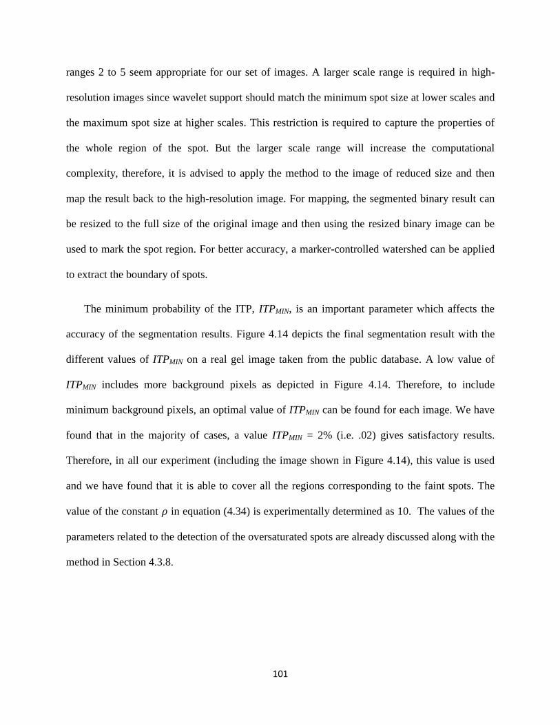
101
ranges 2 to 5 seem appropriate for our set of images. A larger scale range is required in high-
resolution images since wavelet support should match the minimum spot size at lower scales and
the maximum spot size at higher scales. This restriction is required to capture the properties of
the whole region of the spot. But the larger scale range will increase the computational
complexity, therefore, it is advised to apply the method to the image of reduced size and then
map the result back to the high-resolution image. For mapping, the segmented binary result can
be resized to the full size of the original image and then using the resized binary image can be
used to mark the spot region. For better accuracy, a marker-controlled watershed can be applied
to extract the boundary of spots.
The minimum probability of the ITP, ITPMIN, is an important parameter which affects the
accuracy of the segmentation results. Figure 4.14 depicts the final segmentation result with the
different values of ITPMIN on a real gel image taken from the public database. A low value of
ITPMIN includes more background pixels as depicted in Figure 4.14. Therefore, to include
minimum background pixels, an optimal value of ITPMIN can be found for each image. We have
found that in the majority of cases, a value ITPMIN = 2% (i.e. .02) gives satisfactory results.
Therefore, in all our experiment (including the image shown in Figure 4.14), this value is used
and we have found that it is able to cover all the regions corresponding to the faint spots. The
value of the constant 𝜌 in equation (4.34) is experimentally determined as 10. The values of the
parameters related to the detection of the oversaturated spots are already discussed along with the
method in Section 4.3.8.

102
4.3.10.3 Results and Comparisons
The method proposed in this chapter has been applied on the gel images of our data set. For
a comparative analysis, our method is compared with popular commercial software ImageMaster
7 (also known as ImageMaster 7) and a published method in the literature by dos Anjos et al.
[12]. The parameters of the proposed approach have been kept constant throughout the
experiments while the parameters of the commercial software and the method by dos Anjos et al.
[12] were adjusted for each image in order to maximize the detection of the true spots. The
author implementation of the method by dos Anjos et al. [12] – named “SCIMO” is used in our
experiment.
A real gel image and its segmentation results have been depicted in Figure 4.15. SCIMO
method paints the border of spots with yellow color, which is not clearly visible in Figure 4.15.
Therefore, a part of the same gel image and corresponding results are selected and zoomed for
better visibility (see Figure 4.16). It can be observed that ImageMaster 7 seems to include more
background pixels within the spot boundaries while boundaries produced by SCIMO seem to be
more rectangular. The proposed method produces more plausible spot boundaries. For
quantitative analysis, ten synthetic images were created. Since most of the spots in real gel
images can be modeled using 2D Gaussian or 2D flat Gaussian, the synthetic images contain
several 2D Gaussian spots along with 2D flat Gaussian spots in inhomogeneous background
extracted from real gel images using a large size (typically, 50 x 50) mean operator. Some
synthetic images also contain several spots with tails and small streaks. Figure 4.17 and Figure
4.18 show the segmentation results of two synthetic images. It can clearly be observed that our
method produces more plausible spot boundaries.

103
(a) (b)
(c) (d)
Figure 4.14: Effect of different values of ITPMIN on the segmentation result of a real gel image. (a)
ITPMIN = 1% (b) ITPMIN = 2% (c) ITPMIN = 5% and (d) ITPMIN = 10%. Spots identified as the
oversaturated spots are depicted with green border and the rest of the spots are depicted with a
pink border.

104
(a) (b)
(c) (d)
Figure 4.15: (a) a real gel image from public dataset [77] and segmentation results using (b)
Proposed method (c) ImageMaster 7 and (d) SCIMO.

105
(a) (b)
(c)
Figure 4.16: A part of the image and results shown in Figure 5.15(b, c, d) is selected and zoomed for
better visibility. (a) Result by Proposed method (b) Result by ImageMaster 7 and (c) Result by SCIMO.

106
(a) (b)
(c) (d)
Figure 4.17: (a) A synthetic image and its segmentation using (b) Proposed method (c) ImageMaster
7 and (d) SCIMO.

107
(a) (b)
(c) (d)
Figure 4.18: (a) A synthetic image and its segmentation results using (b) Proposed method (c)
ImageMaster 7 and (d) SCIMO.

108
While generating synthetic images, their ground truth images have also been carefully
generated. To compare the segmentation results, a measure of foreground pixels overlap between
ground truth and the result can be a good parameter for evaluation. Each detected spot area is
compared with its ground truth spot area and mean error in spot area for all spots is measured as:
𝐸𝑟𝑟 = 1
𝑁
|𝐷𝑆𝐴𝑖 − 𝐺𝑆𝐴𝑖|
max(𝐷𝑆𝐴𝑖 , 𝐺𝑆𝐴𝑖)
𝑁
𝑖=1
(4.37)
Where DSAi represents the “detected spot area” for an ith
spot in the result, GSAi represents
“ground-truth spot area” for the ith
spot in the ground truth image and N represents the cardinality
of the set 𝐺𝑇𝑓 ∪ 𝑅𝑓 . GTf indicates the set of foreground regions in ground truth image. Rf
shows the set of foreground regions in the obtained segmented result. The operator |.| represents
the absolute value. A zero error will indicate three facts: (1) all spots are segmented (i.e. there is
no spot for which the whole spot area in the result is categorized as background), (2) all spots are
correctly segmented as depicted in the ground truth image and (3) no background region has
been detected as a whole spot. The average of the results of all synthetic images is plotted in
Figure 4.19. The proposed method surpasses the other methods in terms of Err (%). The SCIMO
method results in the highest error since it fails to mark many foreground pixels as spot regions
and thus these spot regions are part of the background in the SCIMO result. ImageMaster 7
detects more background pixels as spot regions and produces almost double the error as
compared to the proposed method. The proposed approach is more conservative in the inclusion
of background regions and provides more accurate results.

109
The stability of the proposed method under different amounts of noise is also studied in this
section. The 2D gel images are produced and acquired using different technological setups or
instruments. While acquiring the image using different setups, different amount of noise may get
introduced in the images. The Segmentation method should be robust to these little noise
variations. Different amount of Gaussian noise (with standard deviations = 1, 2, 3, 4, 5 and 10)
have been introduced in the synthetic images which are then segmented using all the different
methods (the proposed approach, Delta2D, ImageMaster 7 and SCIMO). The parameters of the
proposed approach are kept same throughout the experiment. A change in the parameters of
ImageMaster 7 and SCIMO is always required for correct and optimum results. Here, our
purpose is to visualize the variability among the outputs of a method at different amounts of
noise. Figure 4.20 represents the findings for a synthetic image shown in Figure 4.17 (a). The
Delta2D detects more spots with increasing amount of noise. This may be due to lack of
smoothing parameter in its spot detection module. The proposed approach and SCIMO seem to
Figure 4.19: Mean error in spot area overlap between the segmentation method and ground
truth. The error bar indicates the standard deviation of the corresponding measure (%) across
images in the dataset.
0
5
10
15
20
25
30
35
Proposed
approach
Melanie 7 SCIMO Delta 2DE
rr (
%)

110
have limited variability while the output of ImageMaster 7 seems to be severely affected by
noise.
4.3.10.4 Time Complexity Analysis
The proposed method is based on the undecimated nonseparable wavelet transform. The
time complexity of the decomposition of the wavelet transform is O(N), where N is the number
of pixels in the image. For an Intel ~2 GHz quad-core, 2 GB RAM computer with Windows XP,
the decomposition of the undecimated quincunx transform up to 5 scales takes around 3.5
seconds for a 512 x 512 image.
The maximum size of the neighborhood in equation (4.30) was found to be equal to or less
than 9 x 9 for all gel images during the experiments. Thus, the execution of equation (4.30) takes
less time than the time taken in a convolution operation using a 9 x 9 filter (i.e. less than one
second). The overall execution time of the proposed approach is averaged out to be 12 seconds
which is more than the average time taken by ImageMaster 7 (1 second) and SCIMO (8
seconds). Taking a little more time than the commercial software does not matter to the
Figure 4.20: Effect of different amounts of Gaussian noise on the segmentation results of the
methods.
450500550600650700750800850900950
1 2 3 4 5 10
No
. o
f D
etec
ted
Sp
ots
Standard Deviation of Noise
Proposed
Approach
Melanie 7
SCIMO
Delta 2D

111
biologists since they are more interested in the overall accuracy of the result which saves them a
significant amount of time which goes into the manual editing of the results. It should also be
noted that manual parameter tuning is required in both ImageMaster 7 and SCIMO for producing
optimum results from these methods. The time for tuning the parameters may be a few minutes
to several minutes, while the proposed method either does not require the parameter tuning at all
or requires only a few iterations for selection of the most optimum value of ITPMIN. Therefore,
in the proposed method, only one parameter (or no parameter at all) requires to be tuned which is
easier than tuning three or more parameters (as in the case of ImageMaster 7 and SCIMO).

112
Chapter 5 Segmentation of High-resolution 2DGE Images
5.1 Introduction
Segmentation methods discussed in chapter 4, work well for low-resolution images, but fail
to give a satisfactory performance for high-resolution images. High-resolution images require
decomposing the image into a large number of scales using these methods, which increases
computational complexities. Thus, second segmentation method needs to be modified, so that
decomposition into a large number of scales can be avoided for high-resolution image. Based
upon the observations of the second segmentation method and the spots‟ singularities in the
wavelet domain, it is found out that the sign of wavelet coefficient can play an important role
when the used wavelet is the second derivative of a smoothing function. To cope with the
irrelevant singularities, we proposed the use of kernel density estimator (KDE) at each scale of
the wavelet transform. The advantage of the proposed method is that the number of scales does
not anymore depend upon the resolution or the spot size of the image. The segmentation method
evolved so far still outperforms the other methods and gives satisfactory results.
5.2 Method using Wavelet and Kernel Density Estimation (KDE)
In this work, a novel scheme based on the nonseparable quincunx wavelet transform [69]
[70] is devised to extract all blob regions from the noisy uneven background. A quincunx
wavelet that is the second derivative of a smoothing function provides a multiscale
decomposition of an image, where the sign of the wavelet coefficients are used in a novel fashion
using kernel density estimation technique to categorize the image pixels into darker and brighter
regions. Such formulation brings forward several interesting features which make it
distinguishable from other available methods used for blob segmentation. It can be described as

113
the simplest non-iterative, non-parametric approach which segments out the connected set of
pixels belonging to darker or brighter regions, without relying on any specific initialization
method such as placement of seed points, initial contours and cluster centers. This multiscale
formulation uses a fixed set of scales irrespective of the size and the shape of the blobs. It also
does not depend on the intensity of the blob and can extract even low contrast regions. However,
it is not so effective in the presence of low-contrast noise. In this work, a global threshold is
employed to neglect the low contrast regions. A refinement method consisting of k-means
clustering and region merging is developed to improve the segmentation accuracy of the blob
regions. The performance of the proposed approach is evaluated on synthetic and real images.
The synthetic as well as real 2D gel images are used to demonstrate a possible application of the
proposed segmentation approach in the scientific field. The 2D gel images may contain
overlapping spots and therefore, a method for separation of the overlapping spots is also devised
in this thesis. Experimental results prove that the proposed method is effective for segmenting
the images containing objects of various intensities and shapes.
5.2.1 Foundation
In this section, an image is assumed to consist of blob objects of various sizes, shapes and
intensities in a noisy background (as shown in Figure 5.1). The image segmentation problem is
formulated as the detection and extraction of blob regions from the image.
Let Iσ represent the image 𝐼 ∶ ℝ2 → ℝ at scale σ. In scale-space representation, Iσ is obtained
through the convolution of image I with a Gaussian kernel Gσ.
𝐺𝜍(𝑥, 𝑦) = 1
2𝜋𝜍exp(−
𝑥2 + 𝑦2
2𝜍2)
(5.1)

114
𝐼𝜍 𝑥, 𝑦 = 𝐺𝜍 𝑥, 𝑦 ∗ 𝐼 𝑥, 𝑦 , 𝑥, 𝑦 ∈ ℝ2 (5.2)
The symbol „*‟ denotes convolution.
When a second derivative operator such as Laplacian is applied on an image 𝐼𝜍 , it produces
zero crossing edges. The darker and brighter sides can be differentiated through different signs of
the coefficients of the response.
∇2𝐼𝜍 𝑥, 𝑦 = 𝐿(𝑥, 𝑦) ∗ 𝐺𝜍 𝑥, 𝑦 ∗ 𝐼 𝑥, 𝑦 (5.3)
where L is a Laplacian operator (e.g. 0 1 01 −4 10 1 0
) and the right-hand side of the equation
represents the second derivative of the image I at scale σ. Although, the detection of zero-
crossing edges is a good method to extract the blob regions, the sensitivity of the operator to
noise worsens the situation by producing several false edges and breaking true edges.
Practitioners generally use a threshold to discard noisy edges; however, they find it difficult to
specify a fixed criterion for choosing the threshold in a given set of images. It is a well known
fact that the darker and brighter sides can be differentiated through different signs of the
coefficients of the response of a second derivative operator. Figure 5.2 depicts the positive
signed response of Laplacian operator, which usually occurs on the darker side of the zero-
crossings. For the noisy image, there are several false regions which are detected as darker
(a) (b) (c)
Figure 5.1: (a) A synthetic image of flat objects. (b) A synthetic 2D Gaussian blob image. (c) A noise free
synthetic dark flat top Gaussian blob image.

115
regions. Careful investigation reveals that the density of pixels is more in true blob regions
adjacent to zero-crossings, and this can be used to distinguish true regions from the rest. This
observation is clearly visible at coarser scales (see Figure 5.2).
In another technique usually known as blob detection, the Laplacian of Gaussian (LoG)
operator is applied on the image for a predefined scale range and its response is measured across
the scales. By analyzing maximum response behavior across scale space, blob centre and
corresponding scales are determined [72].
The Hessian matrix for image I is defined as
𝐻 𝑥, 𝑦; 𝜍 =
𝜕2𝐼𝜍(𝑥, 𝑦)
𝜕𝑥2
𝜕2𝐼𝜍(𝑥, 𝑦)
𝜕𝑥𝜕𝑦
𝜕2𝐼𝜍(𝑥, 𝑦)
𝜕𝑥𝜕𝑦
𝜕2𝐼𝜍(𝑥, 𝑦)
𝜕𝑦2
(5.4)
The determinant of the Hessian matrix, det(H) and the trace of the Hessian matrix, trace(H)
have been useful to determine the image feature.
𝑡𝑟𝑎𝑐𝑒 𝐻 𝑥, 𝑦; 𝜍 = 𝜕2𝐼𝜍 𝑥, 𝑦
𝜕𝑥2+
𝜕2𝐼𝜍 𝑥, 𝑦
𝜕𝑦2
(5.5)
= ∇2𝐼𝜍 𝑥, 𝑦 (5.6)
Thus, the trace is simply the response of the second derivative operator on the image.
The darker and brighter blobs usually result in minima and maxima regions respectively in
the gray value image. The minima and maxima of any function can be calculated using Hessian
analysis. If det(H(x,y; σ)) > 0 and trace(H(x,y; σ))>0 then (x,y) is a local minimum of image at
scale σ. If det(H(x,y; σ)) > 0 and trace(H(x,y; σ))<0, then (x,y) is a local maximum of image at

116
scale σ. If det(H(x,y; σ)) < 0, then (x,y) are saddle points are represented. If det(H(x,y; σ)) =0,
any conclusion cannot be drawn with regard to (x,y) being a stationary point. Figure 5.2
represents the minima in Hessian analysis for a darker blob image. When the scale matches the
size of the blob, the region of the blob can be estimated by checking the determinant and trace of
the Hessian matrix. Although, using this technique some false regions are obtained and all the
obtained regions are not exact. Therefore, the obtained regions need to be refined further for
extraction of accurate information (see Figure 5.3). By studying only the trace of the Hessian or
response of the second derivative operator, regions fulfilling the condition of positive trace (i.e.
H(x,y; σ) >0) are extracted and depicted in Figure 5.2. These regions include minimum points as
well as saddle points. These regions contain more connected pixels than the regions obtained
using the condition „det(H(x,y; σ)) > 0 and trace(H(x,y; σ))>0‟. The extraneous pixels in these
regions can be removed in post-processing based on neighborhood region based operations
(similar to the one presented in this chapter). The advantage of this approach is that not all scales
are to be searched and studied for the segmentation of the image containing blobs of various
sizes. Also, it does not require Hessian analysis for blobs at their corresponding scales. The
second derivative operator is applied to the image at some predetermined scale and its response
is studied. „trace(H(x,y; σ))>0‟ represents the positive coefficients of the response of the second
derivative operator at the scale σ. After this, the region is obtained by filtering the positive
coefficients which needs to be post-processed to refine the segmentation.
Since the second derivative operator is sensitive to noise, a region obtained using Hessian
analysis is severely affected by the noises (see Figure 5.2 and Figure 5.3). A close observation
reveals that the density of pixels in the obtained Hessian minima regions is more for true blob

117
regions in comparison with a noisy background. This finding shows that a density based analysis
may improve the obtained result.
Motivated by these observations, in this study, we use a multiscale approach where kernel
density estimation (KDE) [73] technique is applied on each scale to obtain information about
blob regions. Since a wavelet transform is a nonparametric multiscale tool, we use the quincunx
wavelet transform up to a predetermined scale (6 is used in our all experiments). The quincunx
wavelet decomposes the image by a scale of √2. Therefore, a fixed number of decomposition of
images is used to analyze all the images in our experiment. The images contain small as well as
large sized blobs. Figure 5.3 shows the obtained blob regions from a noisy image using the
proposed method.
5.2.2 Wavelet and Blob Regions
When a wavelet is the second derivative of a smoothing function, the zero crossings of the
wavelet transform indicate the points of sharper variation at each scale [74]. The completeness
and stability of different wavelet zero crossing representations have been studied extensively in
[74]-[75]. Zero-crossings in 2D image define a number of connected regions of coefficients
sharing the same sign in the neighborhood. Cvetkovic and Vetterli [75] utilized this information
to build a 2D wavelet zero-crossing representation which was used to reconstruct the image.
Supported by the Hessian analysis in section 5.2.1, the aim of this section is to provide a blob
segmentation method based on the information of the connected regions of coefficients sharing
the same sign.

118
(a) (b) (c) (d)
Figure 5.3: Blob regions obtained using Hessian Analysis at different scales for the noise free and noisy
synthetic image. The region of each blob is obtained at its corresponding scale by searching in the scale
range of σ = 2 to σ = 16 in step of 0.5. (a) Original noise-free synthetic image and (b) blob regions
obtained for noise-free image (c) noisy synthetic image and (d) blob regions obtained for the noisy
image.
(a) (b) (c) (d) (e)
Figure 5.2: Hessian Analysis of a noise free and noisy synthetic image at different scales: σ=2 (first row)
and σ = 6 (second row). (a) Noise free image at specified resolution (b) Hessian minima (regions
satisfying condition: det(H(x,y; σ)) > 0 and trace(H(x,y; σ))>0) for noise-free image (c) positive
Hessian trace (regions satisfying condition: trace(H(x,y; σ))>0) for noise-free image (d) Hessian
minima for noisy image (e) positive Hessian trace for noisy image.

119
The zero-crossings of the discrete wavelet transform can result from the singularities of
either the original signal or the wavelet itself. A regular wavelet will suppress many zero-
crossings while an irregular wavelet will produce many false zero-crossings due to the wavelet
itself. False zero-crossings can be discarded by either neglecting the edges in a low variance area
or using a region based refinement approach similar to the one employed in this section.
Cvetkovic and Vetterli [75] have used a tensor product of one-dimensional regular biorthogonal
wavelet, which favors singularity detection in limited directions (horizontal, vertical and
diagonal). A 2D nonseparable wavelet functions better as a multi-dimensional tool as it captures
the singularities in all directions [34] [35]. The quincunx decomposition being the simplest 2D
nonseparable wavelet is implemented using a lifting scheme [70] for this work. The quincunx
transform has another advantage over separable wavelets in that it provides finer decompositions
of the image by a scale of √2 instead of 2. The undecimated version of quincunx transform is
used to provide the details of the same size as of the image which is required in our analysis.
The lifting framework for undecimated quincunx wavelet is depicted in Figure 5.4. In the
undecimated version of the lifting scheme, instead of subsampling, the predict (P) and update (U)
filters are up-sampled by a dilation matrix 𝐷 = 1 11 −1
in each stage. The scheme with second
order filters has two primal and two dual vanishing moments [70]. The detail part at a lower
branch of the lifting scheme is obtained by subtracting the predicted value from the original
sample (see Figure 5.4). This operation is slightly different from the traditional second derivative
operator (as used in section 5.2.1), where the original sample (centre value) is subtracted from
the predicted value (i.e. weighted sum of neighborhood values). This leads to a sign change. This
also leads to a change in the Hessian condition used to find out region of blobs. Now,
trace(H(x,y; σ))<0 indicates the minimum (or saddle point) at point (x,y) when the second

120
derivative operator is quincunx wavelet. Thus, regions of darker blobs along with some saddle
points can be obtained using the negative signed response of the quincunx wavelet scheme.
5.2.3 Proposed Method
The image is decomposed using the undecimated quincunx wavelet transform up to a
predetermined scale J. In the presence of noise, there will be several zero crossings, several
(a)
(b)
Figure 5.4: Lifting scheme for undecimated quincunx wavelet: (a) analysis and (b) synthesis. Predict (P)
and update (U) filters are upsampled by dilation matrix D. I1 and D1 represent the approximation and
detail part of the next scale and Î represents the reconstructed image. P2 and U2 denote the second
order filters that are used [70].
+
z1-1
+
P2 (ZD) U2 (Z
D)
I
-
+
I1
D1
+
U2 (ZD) P2 (Z
D)
+ z1 +
-
+
I1
D1
Î

121
negative and positive wavelet coefficients at each scale. Consequently, detection of the true zero-
crossing edges will be a difficult task. In this case, one solution is to utilize the underlying
distribution of positive and negative coefficients in the neighborhood of each pixel. We assume
that if the density of negative (positive) signed coefficients is high at a location (x,y), then it is
more probable that the noise-free wavelet coefficient is negative (positive) at this location.
Assuming sign of a wavelet coefficient to be an independent and identical distributed random
variable, the underlying density of negative coefficients at a location (x,y) and scale j can be
given by using the KDE technique [73] as follows:
𝑝𝑗− 𝑥, 𝑦 =
1
𝑁 𝐾 𝑥 − 𝑥𝑖 , 𝑦 − 𝑦𝑖 𝑠𝑖𝑔𝑛
−(𝑤𝑡𝑗(𝑥𝑖 ,𝑦𝑖))
𝑁
𝑖=1
(5.7)
Where
𝐾 𝑥′,𝑦′ =1
𝑑 𝐾(𝑥′/, 𝑦′/)
(5.8)
𝑠𝑖𝑔𝑛− 𝑤𝑡𝑗 ,(𝑥𝑖 ,𝑦𝑖) =
1 𝑖𝑓 𝑤𝑡𝑗(𝑥𝑖 ,𝑦𝑖) < 0
0 𝑜𝑡𝑒𝑟𝑤𝑖𝑠𝑒
(5.9)
The symbol (xi,yi) denotes the location of the ith
neighbor of the wavelet coefficient 𝑤𝑡𝑗(𝑥𝑖 ,𝑦𝑖)
at scale j. The symbol N denotes total number of pixels in the image. The sign- function ensures
that only negative coefficients are weighted according to their spatial distance in the density
estimation. The kernel function K(.) is defined in two-dimensional subspace (i.e., d = 2) and the
scalar h is the kernel bandwidth. The most popular choice is the Gaussian kernel due to its well
known properties of approximations, differentiability, continuity and locality [73]. The two-
dimensional Gaussian kernel with predefined support is written as in equation (5.10).

122
𝐾 𝑥, 𝑦 = 0 𝑖𝑓 𝑥2 + 𝑦2 >
(2𝜋)−𝑑/2 exp −1
2(𝑥2 + 𝑦2) 𝑜𝑡𝑒𝑟𝑤𝑖𝑠𝑒
(5.10)
As assumed, the 𝑝𝑗− 𝑥, 𝑦 will represent the probability that the location (𝑥, 𝑦) belongs to the
spot region. There are two main properties of the wavelet transform: decorrelation of noise
across scales and persistence of significant singularities [28] [31]. The noise has a tendency to
decorrelate itself across scales, while significant singularities have the tendency to propagate
through scales in the wavelet domain. The edges of the spots will produce significant
singularities which may be captured by low wavelet coefficients. For a darker region, high
density of negative wavelet coefficients should be present at all scales near the edges of the
spots, while noise is not supposed to exhibit such type of consistent behavior. Taking the product
of densities across scales will emphasize the consistent behavior across scales and diminish the
effect of noise. Therefore, a multiscale density of the sign of wavelet coefficients at a location
(x, y) can be constructed from the product of scale-wise densities as given in equation (5.11).
𝑥, 𝑦 = 𝑝𝑗− 𝑥, 𝑦
𝐽
𝑗=1
(5.11)
Similarly, the multiscale density of positive sign of the wavelet coefficients at location (x, y)
can be calculated using the same kernel as follows
𝑝+ 𝑥, 𝑦 = 𝑝𝑗+ 𝑥, 𝑦
𝐽
𝑗=1
(5.12)
Where

123
𝑝𝑗+ 𝑥, 𝑦 =
1
𝑁 𝐾 𝑥 − 𝑥𝑖 , 𝑦 − 𝑦𝑖 𝑠𝑖𝑔𝑛
+(𝑤𝑡𝑗 ,(𝑥𝑖 ,𝑦𝑖))
𝑁
𝑖=1
(5.13)
And
𝑠𝑖𝑔𝑛+ 𝑤𝑡𝑗 ,(𝑥𝑖 ,𝑦𝑖) =
1 𝑖𝑓 𝑤𝑡𝑗 ,(𝑥𝑖 ,𝑦𝑖)> 0
0 𝑜𝑡𝑒𝑟𝑤𝑖𝑠𝑒
(5.14)
Clearly, a pixel at location (x, y) has a higher probability to be darker if 𝑝 – 𝑥, 𝑦 > 𝑝
+ 𝑥, 𝑦
or has a greater chance to be lighter if 𝑝 + 𝑥, 𝑦 > 𝑝
– 𝑥, 𝑦 . The plateau region in the image will
have 𝑝 – 𝑥, 𝑦 = 𝑝
+ 𝑥, 𝑦 = 0. Such plateau regions may be merged into the regions just
enclosing them. This way the image can be classified into two distinct groups: lighter and darker.
Suppose the objects are darker than the background then a foreground binary image (B) is
formed as
𝐵 𝑥, 𝑦 = 1 𝑖𝑓 𝑝– 𝑥, 𝑦 > 𝑝+(𝑥, 𝑦)
0 𝑜𝑡𝑒𝑟𝑤𝑖𝑠𝑒
(5.15)
Based on prior knowledge, B can be modified further. In the case of 2D gel images, the
image B is further modified by removing small noisy regions using a morphological opening
operation. A disk shaped structuring element (SERsmall) of radius (Rsmall) equivalent to the radius
of the smallest spot to be detected is used for this purpose. Figure 5.5 shows the corresponding
binary image of a noisy synthetic image.
5.2.4 Region Refinement
The foreground binary image B is the resulting segmented image containing just the protein
spots. The contents of B depend on the kernel bandwidth h that determines the number of details
to be smoothed out. A low value of h will preserve frequent sign changes caused by noise while
a large value of h may overlook the desired details (see Figure 5.5). The value of h is

124
experimentally determined in the experimental section of this thesis. To reduce the chances of
inclusion of extraneous pixels or exclusion of any relevant object pixel in segmentation, the
image B is further refined using a region merging and splitting strategy. The pseudo code of our
algorithm has been given in Figure 5.6.
For each connected region in B, its neighborhood up to a distance (Rn) is merged to make an
extended region. This extended region now includes both lighter and darker pixels. To separate
them out, each extended region is divided into two parts using k-means clustering. We employ k-
means for region splitting because it is a simple, unsupervised and fast technique. If mean gray
values of these two parts are separated by a threshold Th, then only the part having low mean
gray value (in the case of the darker object) is included in final segmented binary image Bf. This
step will exclude any extraneous pixels, if present. The threshold Th is required because all
detected regions may not be of interest and thus, regions showing significant contrast from the
background need to be selected. The pixels that are not included in Bf form the background
region Bg. The connected regions in Bg are found out and added to any adjacent object region of
Bf if the difference between the mean gray value of the adjacent object region in Bf and the mean
(a) (b) (c) (d)
Figure 5.5: Effect of selection of kernel bandwidth on the obtained binary region. (a) Original
synthetic images and obtained binary regions using proposed method at following kernel
bandwidths: (b) h = 1 (c) h = 6 and (d) h = 10.

125
gray value of the region in Bg is less than Th. This way, any excluded object region will be added
back into the final segmented binary image Bf.
The k-means method is simple and does not incorporate any spatial information with image
intensities. In the presence of noise, it may result in segmentation with scattered pixels. A
morphological opening operation (erosion followed by dilation) is required to overcome this
drawback up to some extent. For the morphological opening, a disk-shaped structuring element
(SE1) of radius 1 is used. In Figure 5.6, the symbol „⊝‟ denotes erosion and the symbol „⊕‟
denotes dilation.
5.2.4.1 Separation of Overlapped Spots in 2D Gel Images
The final binary image Bf obtained from above method contains only the foreground pixels.
Some blobs in the image may be overlapped and may be detected as single blob region. These
overlapped blobs may be separated depending upon their structures or features [11] [61] [66]. In
this thesis, we concentrate on the separation of blobs in case of 2D gel images. Several strategies
such as Euclidian distance, regional minima in large neighborhoods and spot modeling have been
employed by researchers. The modeling of spots is a time consuming task due to the presence of
several spots in 2D gel images. The Euclidian distance based method results in over-
segmentation of irregularly shaped spots, while the method depending upon regional minima
results in over-segmentation of noisy spots due to the presence of several false regional minima.
To improve the situation, both Euclidian distance and regional minima are utilized together to
split the overlapped spots. The pseudo code of the algorithm has been depicted in Figure 5.7. The
spot centers are estimated by finding the local maxima of the Euclidian distance transform (EDT)
applied on the binary image Bf. The false adjacent local maxima are merged into one large region

126
using the morphological dilation operator. The dilation operator is applied using the disk-based
structuring element (SERsmall) of radius Rsmall. The spot centers are also estimated by finding the
regional minima in median filtered gray value image. The disk-shaped neighborhood of radius
Rsmall is used to find out the regional minima. To reduce the false regional minima due to noise,
the median filtered image is used. To remove the false minima that may occur near spot edges,
the binary image Bf is eroded using the disk-shaped structure SERsmall. The regional minima that
fall in the foreground region of the eroded binary image are kept as estimated spot centers. The
adjacent false regional minima are merged together into one large region by applying the
morphological dilation operator using the disk-shaped structuring element SERsmall. If a dilated
region of a regional minimum of median filtered gray value image overlaps with dilated local
maxima of Euclidian transform, the dilated region of the regional minimum is considered as a
valid spot center (step 6 in Figure 5.7). Such spot centers are imposed as minima markers in the
gradient of the binary image Bf and the watershed transform is applied to find out the common
boundary between the overlapped spots. Figure 5.8 depicts the separation of overlapped spots.
The proposed approach results in better separation of spots and is more robust to multiple
regional minima and irregular shape of spots.

127
1. 𝑓𝑜𝑟 𝑒𝑎𝑐 𝑐𝑜𝑛𝑛𝑒𝑐𝑡𝑒𝑑 𝑟𝑒𝑔𝑖𝑜𝑛 𝐶𝑖 𝑖𝑛 𝐵
2. 𝐶𝑖−𝑒𝑥𝑡𝑒𝑛𝑑𝑒𝑑 = 𝐶𝑖 ∪ 𝑁𝑒𝑖𝑔𝑏𝑜𝑟𝑠𝑢𝑝𝑡𝑜 _𝑑𝑖𝑠𝑡𝑎𝑛𝑐𝑒 _𝑅𝑁
3. 𝑑𝑎𝑟𝑘𝑒𝑟𝑚𝑒𝑎𝑛 ,𝑑𝑎𝑟𝑘𝑒𝑟𝑟𝑒𝑔𝑖𝑜𝑛 ,𝑏𝑟𝑖𝑔𝑡𝑒𝑟𝑚𝑒𝑎𝑛 = 𝑠𝑝𝑙𝑖𝑡𝑘𝑚𝑒 𝑎𝑛𝑠 𝐶𝑖−𝑒𝑥𝑡𝑒𝑛𝑑𝑒𝑑
4. 𝑖𝑓 𝑏𝑟𝑖𝑔𝑡𝑒𝑟𝑚𝑒𝑎𝑛 – 𝑑𝑎𝑟𝑘𝑒𝑟𝑚𝑒𝑎𝑛 > 𝑇 𝑡𝑒𝑛
5. 𝐵𝑓 = 𝐵𝑓 ∪ 𝑑𝑎𝑟𝑘𝑒𝑟𝑟𝑒𝑔𝑖𝑜𝑛
6. 𝑒𝑛𝑑 𝑖𝑓
7.𝑒𝑛𝑑 𝑓𝑜𝑟
8.𝐵𝑔 = 𝐵 − 𝐵𝑓
9.𝑓𝑜𝑟 𝑒𝑎𝑐 𝑐𝑜𝑛𝑛𝑒𝑐𝑡𝑒𝑑 𝑟𝑒𝑔𝑖𝑜𝑛 𝐷𝑖 𝑖𝑛 𝐵𝑔
10. 𝑓𝑖𝑛𝑑 𝑎𝑙𝑙 𝑓𝑜𝑟𝑒𝑔𝑟𝑜𝑢𝑛𝑑 𝑟𝑒𝑔𝑖𝑜𝑛𝑠 𝐹𝑖 ∈ 𝐵𝑓 , 𝑡𝑎𝑡 𝑎𝑟𝑒 𝑎𝑑𝑗𝑎𝑐𝑒𝑛𝑡 𝑡𝑜 𝐷𝑖
11. 𝑓𝑜𝑟 𝑒𝑎𝑐 𝐹𝑖 𝑎𝑑𝑗𝑎𝑐𝑒𝑛𝑡 𝑡𝑜 𝐷𝑖
12. 𝑖𝑓 𝑚𝑒𝑎𝑛𝑔𝑟𝑎𝑦𝑣𝑎𝑙𝑢𝑒 𝐹𝑖 − 𝑚𝑒𝑎𝑛𝑔𝑟𝑎𝑦𝑣𝑎𝑙𝑢𝑒 𝐷𝑖 < 𝑇 𝑡𝑒𝑛
13. 𝐹𝑖 = 𝐹𝑖 ∪ 𝐷𝑖
14. 𝑒𝑛𝑑 𝑖𝑓
15. 𝑒𝑛𝑑 𝑓𝑜𝑟
16. 𝑢𝑝𝑑𝑎𝑡𝑒 𝐵𝑓 𝑤𝑖𝑡 𝑚𝑜𝑑𝑖𝑓𝑖𝑒𝑑 𝐹𝑖
17. 𝑒𝑛𝑑 𝑓𝑜𝑟
18. 𝐵𝑓 = 𝐵𝑓 ⊝ 𝑆𝐸1 𝑆𝐸1
Figure 5.6: Pseudo code of the Region Refinement method.

128
//Estimating the spot center using Euclidian distance
1. 𝐸1 = 𝑙𝑜𝑐𝑎𝑙𝑚𝑎𝑥𝑖𝑚𝑎 𝐸𝐷𝑇 𝐵𝑓
2. 𝐸1𝐷 = 𝐸1 𝑆𝐸𝑅𝑠𝑚𝑎𝑙𝑙
//Estimating the spot centers using regional minima of gray value image
3. 𝐸2 = 𝑟𝑒𝑔𝑖𝑜𝑛𝑎𝑙𝑚𝑖𝑛𝑖𝑚𝑎𝑅𝑠𝑚𝑎𝑙𝑙 𝑚𝑒𝑑𝑖𝑎𝑛 𝐼
4. 𝐸2′ = 𝐸2 ∩ 𝐵𝑓 ⊝ 𝑆𝐸𝑅𝑠𝑚𝑎𝑙𝑙
5. 𝐸2𝐷 = 𝐸2
′ ⊕ 𝑆𝐸𝑅𝑠𝑚𝑎𝑙𝑙
6. 𝑣𝑎𝑙𝑖𝑑 𝑠𝑝𝑜𝑡 𝑐𝑒𝑛𝑡𝑒𝑟𝑠 = 𝑝 ∈ 𝐸2𝐷 𝑞 ∈ 𝐸2
𝐷 ∩ 𝐸1𝐷 𝑎𝑛𝑑 𝑞 ⊆ 𝑝}
7. 𝐺 = 𝑔𝑟𝑎𝑑𝑖𝑒𝑛𝑡 𝐵𝑓
// Mark valid spot centers as minima marker by assigning them minimum value
8. 𝐺 𝑣𝑎𝑙𝑖𝑑 𝑠𝑝𝑜𝑡 𝑐𝑒𝑛𝑡𝑒𝑟𝑠 = −𝐼𝑛𝑓𝑖𝑛𝑖𝑡𝑦
9. 𝐿 = 𝑤𝑎𝑡𝑒𝑟𝑠𝑒𝑑(𝐺)
//L is the final segmented image.
Figure 5.7 Pseudo code for separation of overlapped spots in 2D gel image.

129
5.2.5 Experimental Results and Discussion
The performance of the proposed method is demonstrated using the following different types
of images: (1) synthetic images containing flat objects of different shapes and sizes, (2) synthetic
images containing 2D Gaussian blobs, (3) real 2D gel images and (4) other biological images.
Only synthetic images are used to measure the performance quantitatively. An example of them
is shown in Figure 5.1. To measure the accuracy of segmentation of synthetic images, Jaccard
Distance (JD) error metric is used and defined as 𝐽𝐷(𝑆, 𝐺) = (1 − | 𝑆 ∩ 𝐺 | 𝑆 ∪ 𝐺 ) , where S
is the segmented result and G is ground truth reference. The operator |.| denotes the number of
elements (pixels) in the set. To find the percentage of correctly classified pixels in the image, a
metric called „segmentation accuracy index‟ is also defined as 𝑆, 𝐺 = 𝑆 ∩ 𝐺 + 𝑆𝐵 ∩
𝐺𝐵 / ( 𝑖𝑚𝑎𝑔𝑒 𝑠𝑖𝑧𝑒) . The symbols SB and G
B denote the set of background pixels in the
segmented result and ground truth reference respectively. Both JD and SA vary between 0 and 1.
For correct segmentation, JD should be low and SA should be high. For the real 2D gel images,
the ground truth is generally difficult to find out and can be estimated using the consensus of
expert biologists. Still, the variability in different manual segmentations for the same image
cannot be ignored [76]. The relative comparisons between the obtained segmentation results
(a) (b) (c) (d)
Figure 5.8: (a) Protein spots from real image and separation of overlapped spots after segmentation,
using (b) Euclidian distance, (c) regional minima and (d) proposed approach.
130
using different methods for the 2D gel images is qualitatively studied using close observations
done by human experts.
Parameter Determination
The parameters used in the proposed methods are number of scales J, kernel bandwidth, h,
neighborhood distance, RN and threshold, Th. The number of scales 𝐽 = 6 is found to be
sufficient to capture the entire information in an image. In quincunx domain, a scale 𝐽 = 6
corresponds to scale 3 of the separable wavelet, since quincunx wavelet decomposes the image
by a scale factor of √2 instead of 2. The neighborhood distance, RN , defines the locality of the
blob region. A high value of RN indicates that the nature of segmentation is more global while a
low value of RN indicates that the nature of segmentation is more local. Based on the study of
synthetic and real images (see Figure 5.9), RN = 2 stands for the most obvious choice.
The threshold Th defines the contrast of the blob object to be detected. For the images
containing low contrast blob objects, this value should be small. For the images containing only
high contrast blob objects, this value should be large. Our synthetic and gel images contain blob
objects of various intensities in a noisy or inhomogeneous background. We choose 𝑇 = 6 for
these types of images. For other types of biological images, the set of suitable parameters is
obtained by experimenting on a few images. After that, the parameters remain fixed for that set
of images.
The kernel bandwidth h depends upon the details to be extracted out and thus, depends on
the size of blobs and amount of noise. For the images containing very low amount of noise, this
value can be as low as = 1. For images containing high amount of noise or inhomogeneous
background, this value should be sufficient to cope with the noise or inhomogeneity. Although,

131
when blob size is small, a large value of h may smooth out small blobs and may fail to detect
them (see Figure 5.4). For our set of synthetic images, we plot the segmentation accuracy index
SA for each choice of the value of h (see Figure 5.10). It is clearly visible that = 6 is a good
choice for these types of images. Since spots in the real gel images are usually modeled using 2D
Gaussian or flat 2D Gaussian, the real gel images may be assumed to be similar to our synthetic
images of Gaussian blobs. Therefore, the value of h is chosen as 6 real images too. The real 2D
gel images available on public databases (e.g. [77]) are of low-resolution and contain several
blobs of small sizes. A high value of kernel bandwidth h = 6 may overlook many small sized
spots. Therefore, for such images, a low value of h (h = 1) is used to detect blobs. The images in
the last set are noise-free, therefore, a low value of h (h = 1) is preferred.
Quantitative and Qualitative Analysis
The proposed method is applied on the synthetic image shown in Figure 5.1(a) and a set of
other biological images (see Figure 5.11). The fluorescence microscopic cell image (shown in
Figure 5.11(b)) contains several blobs of the same size [79]. The LoG method [72] is generally
used to find the centers of the blobs. The region of blobs can be segmented using the proposed
approach. For the red blood cell images infected with malaria parasites, the detection and
segmentation of the dark structures [78] is important. With a low value of threshold Th, the
proposed approach can detect all cells along with dark cells. To detect only dark cells, the
threshold Th is increased from 6 to 45. Figure 5.11(c) depicts the segmentation results obtained
using proposed approach.
Due to the presence of an uneven background, the general purpose methods are not sufficient
to segment the synthetic images consisting of 2D Gaussian blobs and real 2D gel images (see
132
Figure 5.9 (f)). Therefore, application specific methods available in the literature, as described in
section 5.1, need to be compared with our methods. The methods based on watershed [12] and
Otsu‟s threshold [13] has been used to compare our results. The proposed method is also
compared with two commercial software packages (Delta2D and ImageMaster 7) for 2D gel
image analysis. The parameters of the watershed method [12] have been adjusted for each
image. The parameters of Otsu‟s threshold method [13] have been selected as mentioned in the
paper [13]. The parameters of the commercial software have been adjusted for each image. The
parameters of the proposed method for 2D gel images are selected as described in section 5.2 and
are kept constant throughout the experiment.
All synthetic Gaussian blob images have been subjected to a small amount of Gaussian (with
a standard deviation between 1 and 5) and salt and pepper (1%-3%) noise to simulate the noise in
original gel images. The segmentation results of a synthetic Gaussian blob image are shown in
Figure 5.12. Watershed method [12] does not cope well enough with salt and pepper noise;
therefore the image is filtered using a 3 x 3 median filter before applying this method. Delta2D
has a manual preprocessing operation for removing white and black speckles which has been
utilized for obtaining a better result. By observing Figure 5.12, it can easily be concluded that the
boundary produced by our method is more compact and contains only a few background pixels.
The ground truth image has been formed by assuming the spot boundaries at a distance of two
standard deviations from the spot‟s center and is depicted in Figure 5.13. This assumption is
normal in our case since most of the methods developed for 2D gel images produce large spot
regions in the segmentation for the most of the spots (see Figure 5.12 and Figure 5.15). A total of
90 true spots are present in this image (see Figure 5.12(a) and Figure 5.13).

133
(a) (b) (c)
(d) (e) (f)
Figure 5.9: Effect of the parameter RN on the final segmentation. (a) A 2D gel image and (b)-(e)
segmented results using our method when RN was set to 2, 5, 10 and 15 respectively. As value of RN
increases, region of blobs spreads out and may merge nearby blobs. It leads to more global
segmentation. (f) Segmentation by a global method – active contour [7].

134
Figure 5.10: Plot of kernel bandwidth (h) vs. average segmentation accuracy SA (%) for six synthetic
images. Images are corrupted with Gaussian noise (with a standard deviation between 1 and 5) and
salt and pepper (1%-3%). Example of synthetic images containing 2D Gaussian blobs is shown in
Figure 5.21(b). Solid line represents average SA for all images.
86
87
88
89
90
91
92
93
94
95
96
0 1 2 3 4 5 6 7 8 9
SA (
%)
Kernel Bandwidth (h)

135
To provide an in-depth analysis, the total number of detected spots along with the number of
artifacts and the number of missed spots is also considered for result comparison. The proposed
method detects total 93 spots along with 4 artifacts (background region detected as a spot). It
also fails to detect one true spot. The watershed method [12] and Otsu‟s threshold method [13]
miss more spot regions (15 and 10 spot regions respectively) and detect more number of artifacts
too (11 and 12 false spot regions respectively). Total 86 spots are detected by the watershed
method [12]. Otsu‟s threshold method [13] detects total 89 spots with 2 overlapped and 4 over-
segmented spot regions. Many regions are over-segmented by Delta2D due to the presence of
noise. It also fails to detect 3 true spots. Image Master 7 detects total 88 spots with 4 artifacts and
5 overlapped spot regions. One spot is over-segmented too. Both, the proposed approach and
(a) (b) (c)
Figure 5.11: Original synthetic/ real images (first row) and segmentation results obtained using
proposed approach ( second row).

136
ImageMaster 7 detect less number of artifacts and miss less number of spots in comparison with
the others. The boundaries produced by ImageMaster 7 are much further away from the actual
spot boundaries. Overall, the proposed method produces the least segmentation error and detects
the most number of true spots for the synthetic Gaussian blob images (see Figure 5.14).). The
terms „JD (%) – Worst‟ and „SA (%) – Worst‟ used in Figure 5.14 (a) denote the metrics JD and
SA respectively for the segmentation of such images. Since the segmentation of the synthetic
Gaussian blob images presents a challenging situation for the commercial software packages, the
segmentation analysis of another type of synthetic images is necessary. The best case may be a
noise free image consisting of dark flat top Gaussian blobs with distinct boundaries (see Figure
5.11(c)). The segmentation of such images is easy and can also be easily carried out with any
known methods [51] [53] [55]. The segmentation of such images presents an „easy case‟ or a
„best case‟ scenario for our experiments. All the methods produce accurate segmentations for
such images. The terms „JD (%) – Best‟ and „SA (%) – Best‟ used in Figure 5.15 (a) denote the
metrics JD and SA respectively for the segmentation of such images. Since all the spots are
correctly detected in the „best case‟ scenario, the Figure 5.15 (b) represents only the case of
segmentation of synthetic Gaussian blobs („worst case‟ scenario). The proposed method
produces the least difference between best case and worst case segmentation scenarios among all
the methods (see Figure 5.14(a)). In terms of number of segmented spots, the performance of the
proposed method is comparable with the commercial software packages (see Figure 5.14 (b)). In
brief, the proposed method produces the least segmentation error, detects a smaller number of
artifacts and misses a smaller number of spots as compared to commercial software.

137
Figure 5.13: Boundaries of the spots are assumed at a distance of two standard deviations from
their center.
(a) (b) (c)
(d) (e) (f)
Figure 5.12: (a) A synthetic image consisting 2D Gaussian blobs and its segmentation results using (b)
the proposed approach, (c) watershed method, (d) Otsu’s threshold, (e) Delta2D and (f) Image
Master 7.

138
Figure 5.15 and Figure 5.16 depict the segmentation results of real 2D gel sub-images. The
proposed method provides more plausible boundaries of the spots. The proposed method also
seems to produce less number of artifacts caused due to streaks and background intensity
variations. The Otsu‟s threshold [13] detects several implausible spots for the sub-image shown
in Figure 5.16. Delta2D and ImageMaster 7 seem to detect more number of implausible spots on
the streaks than the proposed method for the sub-image shown in Figure 5.16. The boundary
produced by ImageMaster 7 is less accurate than the proposed method.
The source code of the proposed method can be downloaded from
http://www.mathworks.com/matlabcentral/fileexchange/48610-wavelet-based-noise-robust-
image-segmentation. The proposed approach is planned to be implemented in the advanced
version of our spot picker robot system.

139
(a)
(b)
Figure 5.14: Comparison of different segmentation methods for synthetic Gaussian blob images. (a)
The segmented spot regions are evaluated using the terms JD and SA. (b) The number of segmented
spots is evaluated as a fraction of the total number of true spots in ground truth.
0%
10%
20%
30%
40%
50%
60%
70%
80%
90%
100%
Proposed method Watershed Otsu's Threshold Delta 2D Image Master 7
SA -worst JD -worst
0%
20%
40%
60%
80%
100%
120%
Proposed
method
Watershed Otsu's
Threshold
Delta 2D Image Master
7
Artifacts
Oversegmented
Missed
Overlapped
Correctly-detected

140
(a) (b)
(c) (d)
(e) (f)
Figure 5.15: (a) Real 2D gel sub-image and segmentation results using (b) proposed approach, (c)
watershed, (d) Otsu’s threshold, (e) Delta2D and (f) ImageMaster 7.

141
(a) (b)
(c) (d)
(e) (f)
Figure 5.16: (a) Real 2D gel sub-image and segmentation results using (b) proposed approach, (c)
watershed, (d) Otsu’s threshold, (e) Delta2D and (f) ImageMaster 7.

142
5.2.6 Detailed Results on Synthetic Image
The first set of synthetic images is segmented with the traditional global k-means method as
well as with the state-of-the-art region based segmentation methods, namely, Chan-Vese active
contour (CV) [55] and Kernel Weighted Fuzzy C-Means incorporating local information
(KWFCM) [52]. These methods have been applied to a synthetic image shown in Figure 5.18
and the obtained segmentation errors have been plotted in Figure 5.17. The proposed approach
produces, overall, the least segmentation error and thus, outperforms these methods. The
synthetic image has various objects of different intensities and shapes. The result shown in
Figure 5.17 also reflects that the proposed method is less sensitive to image noise and can
provide better segmentation even when low-intensity objects are present. Global methods don‟t
produce accurate segmentation results of 2D gel images shown in Figure 5.19.
Some natural images containing objects which are either darker or lighter as compared to
their local background are selected from a public database [77]. Figure 5.20 show that the
proposed method provides more desirable segmentation with less number of background pixels.
In this chapter, a novel wavelet based method for accurate and noise robust image
segmentation is presented. The method is formulated upon a subjective criterion that blob objects
are either darker or lighter than their local background. The darker or brighter regions are
extracted by comparing the multiscale density of the signs of wavelet coefficients and are further
refined using a region splitting and merging strategy. Experimental results show that proposed
approach outperforms the state-of-the-art methods. Its application on 2D gel images
demonstrates that this method may prove as a powerful tool for the segmentation of other similar
scientific images.

143
Table 5.1 Detailed result on synthetic image
Original image Bandwidth
(h)
Darker regions, lighter
regions and plateau
regions indicated by black,
white and gray color
respectively.
Effect on Final
segmentation
Parameters for synthetic
image :RN =2, Th=6
Noise free synthetic
image
1
1

144
Synthetic image
corrupted with an
additive Gaussian noise
of standard deviation σn
= 40.
3
6
(see the
corner of
the star and
smooth
background
)
9

145
Noisy synthetic image corrupted with the
additive Gaussian noise of standard deviation
σn =20.
The proposed approach produces the least
error among the methods presented here. (JD
Error =0.46%, execution time=8.5 seconds)
Figure 5.17: Segmentation errors for the image of Fig. 5.21(a) with different methods. The horizontal
axis represents the standard deviation of Gaussian noise in the image.
0
1
2
3
4
5
6
7
8
20 30 40
JD E
rro
r (%
)
Wavelet
CV
KWFCM
K-means
(a)
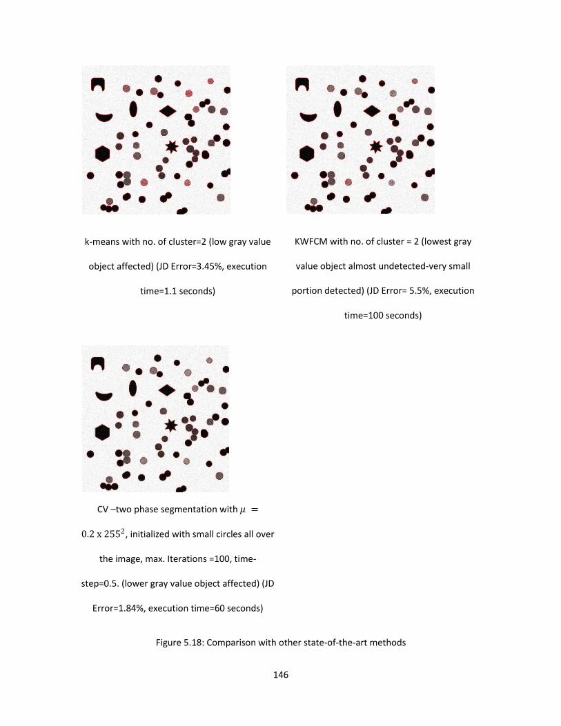
146
k-means with no. of cluster=2 (low gray value
object affected) (JD Error=3.45%, execution
time=1.1 seconds)
KWFCM with no. of cluster = 2 (lowest gray
value object almost undetected-very small
portion detected) (JD Error= 5.5%, execution
time=100 seconds)
CV –two phase segmentation with 𝜇 =
0.2 x 2552, initialized with small circles all over
the image, max. Iterations =100, time-
step=0.5. (lower gray value object affected) (JD
Error=1.84%, execution time=60 seconds)
Figure 5.18: Comparison with other state-of-the-art methods

147
Figure 5.19: First Row: CV method on synthetic and real 2D gel images.
Second Row: KWFCM method on the same synthetic and real 2D gel
images
(a) (b)
(c) (d)
Figure 5.20: (a) An image from the public database and its segmentation using (b) Proposed approach
(c) CV and (d) KWFCM.

148
Conclusion
The proposed strategy for 2D gel electrophoresis image analysis from denoising to
segmentation of the protein spots has been explained for the extraction of true protein spots. The
proposed novel approaches based on nonseparable wavelet decomposition have been
implemented for better characterization of the interior regions and the edges of the protein spots
and for removal of artifacts and streaks.
In this work, a successful attempt has been made to utilize advantages of various wavelet
based methods to move towards a more reliable and accurate technique for denoising of
proteomic 2DGE images. Separable wavelets are tensor product of 1D wavelets and can't carry
much directional information. Nonseparable wavelets are directional and therefore they capture
directional information more efficiently. This property has been utilized for the denoising of
2DGE images in our work. From our experiments, we observed that superb results were obtained
on using undecimated quincunx wavelet with Bayes threshold.
In order to provide better segmentation results, the behaviour of spots, background and
streaks has been analyzed in nonseparable wavelet domain. Three methods have been
systematically developed by addressing problems one by one. Each method provides different
insights to the analysis of 2D gel images and nurtures the understanding of the problems to be
solved. In the first method, the behaviour of streaks is analyzed in a combined domain of
watershed and wavelets that primarily helps in the segmentation of protein spots. The presence
of faint spots and artifacts is another big challenge in the segmentation process which demanded
a different approach. For this purpose, a novel wavelet inter-scale ratio was derived to
characterize the spots interior region in the second method. The method successfully segments
149
the spots from an inhomogeneous background using a fixed global threshold. Reducing
computational complexity and number of artifacts was again a challenge. The multi-scale kernel
density estimation of wavelet coefficients across scales was derived for this purpose and was
utilized to formulate our third segmentation method which provides the most robust and
sophisticated solution for high-resolution images. The experimental results shown in this thesis
demonstrate that the efficiency and accuracy of the proposed approaches is better than
commercially available software and previously reported works.
Registration is an important part of 2DGE image analysis work flow. Image Registration is a
process that involves aligning of two or more images with respect to a reference image using
geometric transformations applied on target images. Registration methods usually require feature
points which depend upon the accuracy of segmentation. A less accurate segmentation provides
erroneous feature points and leads to errors in registration. The proposed segmentation
algorithms are also helpful for providing more accurate registration as discussed in Appendix I.
The proposed methods are incorporated in our Spot Picker Robotic System [2] for laboratory
demonstration. The Spot Picker Robotic System is a state-of-the-art technology for precise
detection, positioning and excision of protein spots from 2D gel images. It can play a pivotal role
in the field of proteomics by using powerful imaging algorithms to help discover new drugs and
biomarkers for early disease diagnosis.
Differential analysis and selection of significant spots for excision are critically important for
comparison between samples from a healthy and a diseased person. Our future work will
concentrate on developing advanced methods for the registration and differential analysis of
2DGE images and building a spot classifier for a complete and fast automation of the system.

150
Appendix I 2DGE Image Registration
I.1 Introduction
Image Registration is a process that involves aligning of two or more images with respect to
a reference image using geometric transformations applied on target images. Misalignment of
images may be due to a variety of reasons like a change in camera perspective, lens distortion
etc. Image matching in 2D gel analysis is used for finding out identical proteins in two or more
gel images. But due to gel to gel variations and presence of noise, this task becomes complicated.
Any protein may not be at the same pixel location in the two images and even size variations
may occur. Existing software packages like ImageMaster 7 and Delta2D are semi-automated and
require significant human intervention to achieve better results. A gel pair may take 4-6 hours of
manual spot matching corrections with current software packages. Hence, manual analysis of
these complex gel images is a significant bottleneck in the proteomics research field, which can
be alleviated by improved and efficient automatic registration techniques. When several gel
images have been matched, a single synthetic gel image can be generated which combines the
information from the individual images in an optimal way. This synthetic gel should consist of a
representative set of spots generated from several registered gel images. The merging process
needs to take the shape information of registered spots into account and can also be used as a
reference gel to perform further registration against unknown gel images. After alignment, there
may still be differences in regions where proteins appear or disappear, and the shape and/or size
of each spot could be different. These regions may form outliers that need to be examined
further.

151
I.2 Registration Techniques
2DE gel registration can be done either using algorithms driven directly from image metrics
or using point set registration techniques. The former technique is known as intensity based
while the latter is known as feature based. Both these techniques start with referring one gel
image as the reference or fixed image and others gel images are called target gel images.
I.2.1 Intensity Based
Intensity-based methods compare intensity patterns in images via image metrics. These
algorithms share the common framework depicted in Figure I.1. Image registration is the process
of finding a coordinate transformation function T(x), given by equation (I.1)
𝑇 𝑥 :ℛ2 → ℛ2 (I.1)
which maps the spatial coordinates from one image I1(x) onto another image I2(x), so that
I2(T(x)) is spatially aligned with I1(x). Mathematically, the registration problem is formulated as
an optimization problem:
argmink
𝐶 𝑇𝑘 , 𝐼1, 𝐼2 (I.2)
where C denotes a cost metric and vector k contains parameters of the transformation function T.
C contains two parts, similarity measure and regularization term. We have employed normalized
mutual information [84][88] as a similarity measure and the smoothness constraint as
regularization term. The transformation function is expressed as a linear combination of B-spline
basis functions of order 3, placed on a regular control point grid.

152
𝑇𝑘 𝒙 = 𝑐1(𝑖, 𝑗)
𝑐2(𝑖, 𝑗)
𝑖 ,𝑗
𝛽3 (𝑥
𝑠𝑥− 𝑖)𝛽3 (
𝑦
𝑠𝑦− 𝑗)
(I.3)
Cost metric C is minimized using the Broyden-Fletcher-Goldfarb-Shanno (BFGS) iterative
optimization method.
Figure I.1: Registration Framework
Figure I.2: Image registration result Figure I.3: Segmentation after image registration
The experimental image is displayed with pure green color (figure I.2 and I.3). The reference
image is displayed with pure magenta color. The experimental image is overlaid on the reference
image. Proteins which are present in both gels are represented using a dark color (dark green to
black). The darkness of the colour depends upon the concentration of proteins. Algorithms
driven by image metrics like mutual information and sum of squared distances (SSD) generate a
Source image
Target image
Transform
Interpolator
Cost metric Optimizer
Similarity Measure Regularization Term

153
subspace containing many local minima for small spot features and these algorithms are not
sufficiently robust against these minima [86].
I.2.2 Point Set Registration
Point set registration is the process of aligning two point sets. These point sets are comprised
of protein spot information, extracted using the segmentation algorithms discussed in chapter 5.
Individual spot parameters like centroid, size, area, intensity, coefficient of variation etc. are
calculated for each spot. Given two sets of points, 𝑥 = (𝑥1, 𝑥2 , … . , 𝑥𝑁)𝑇 and
𝑦 = (𝑦1,𝑦2, … . , 𝑦𝑀)𝑇, where 𝑁 , 𝑀 is the number of points in 𝑥 and 𝑦 respectively. 𝑥𝑖 =
(𝑥𝑖1, 𝑥𝑖2) and 𝑦𝑖 = (𝑦𝑖1,𝑦𝑖2) ,our aim is to find out the correspondence matrix 𝑚 of size 𝑁 × 𝑀
and transformation 𝑇 that minimizes equation (I.4) [86]
𝐸 𝑚. 𝑇 = 𝑤𝑖 𝑥𝑖 − 𝑇 𝑦𝑖′
𝑇𝑆𝑖
−1 𝑥𝑖 − 𝑇 𝑦𝑖′ + 𝜆𝐽𝑇
𝑁
𝑖=1
(I.4)
where
𝑦𝑖′ =
𝑚𝑖𝑦
𝑚𝑖𝑗𝑗 , 𝑤𝑖 = 𝑚𝑖𝑗
2
𝑗
(I.5)
and
𝑆𝑖 = 𝑚𝑖𝑗 (𝑆𝑖 ,𝑥 + 𝑆𝑗 ,𝑦) / 𝑚𝑖𝑗
𝑗
(I.6)
𝑚 is the correspondence matrix with values in the range [0, 1], representing the confidence
of each possible correspondence between 𝑦𝑖 and 𝑥𝑖 . 𝑦′ and 𝑤, respectively, are the weighted
mean location and combined weight for a weighted combination of original points 𝑦. Covariance

154
matrices 𝑆𝑖 ,𝑥 and 𝑆𝑗 ,𝑦 represent uncertainty on the location of each point. The last term 𝐽𝑇
represents transformation smoothness [86]. Closed form solution of equation (I.4) doesn‟t exist
and parameter 𝜆 provides a trade-off between smoothness and accuracy of matching. Iterated
closest point (ICP) [87] based algorithm can be used in an iterative fashion to find out the best
match. General ICP algorithm is depicted in figure I.4. ICP based algorithm consist of a distance
metric, correspondence matrix and transformation function [86]. Distance metrics that can be
used are Euclidean distance, shape context [85], mahalanobis distance etc. Shape context (SC)
[85] provides a semi-global description of the spatial distribution of neighbouring points by
counting the number of points in radial regions, yielding histograms that can be made invariant
to affine deformations. Correspondence matrix 𝑚 can be calculated from the distance metric
using a variety of methods like closest point, kCP, SoftAssign [90] and Bi-partite graph matching
[85]. Bi-partite graph matching ensures one to one correspondence. Finally, the transformation
matrix is calculated by using initial point and correspondence and the target points are mapped to
new points. Techniques exist in literature to find out closed form solutions to calculate
transformation parameters like iterative M-estimation using residual distance distribution (M-
estimator) [89]. The Shape context (SC) [85] based method with thin plate spline as
transformation is applied to two gel images and the results obtained are depicted in figure I.5.
Segmentation method discussed in chapter 5 is deployed to find out the protein spots in two
gel images and then SC method is applied on the pair of gel images. Matching results are shown
in figure I.5. Match vectors are shown in the target image in green color.

155
Figure I.4: ICP algorithm
Point Sets :( x, y), T
Distance Metric
𝑥, 𝑦′ → 𝐷𝑖𝑠𝑡
Correspondence
𝐷𝑖𝑠𝑡 → 𝑚
Transformation
𝑥, 𝑦′ ,𝑚 → 𝑇
Converged?
T
Yes
No
Mapping 𝑦 𝑇→ 𝑦′

156
Figure I.5 SC[85] method results. T1_Gel3 is reference gel image and T1_Gel1 is target gel image. Match
vectors are shown in green color.

157
References [1] Marc R. Wilkins, Christian Pasquali, Ron D. Appel, KeliOu, Olivier Golaz, etal., “From
Proteins to Proteomes: Large Scale Protein Identification by Two-Dimensional
Electrophoresis and Amino Acid Analysis,” Nature Biotechnology, Vol.14, No. 1, pp. 61-
65, 1996.
[2] "Development of Spot Picker Robot for Proteomics Applications", Ratnesh S Sengar,
A.K Upadhyay, D.N.Badodkar, R.K.puri, Manjit Singh, MGR Rajan, Vikram M
Gadre, IEEE International Conference on Robotics & Automation (IEEE-ICRA2013) at
Karlsruhe, Germany, DOI: 10.1109/ICRA.2013.6630801, pp 1704-1709., [2013].
[3] Thierry Rabilloud, Cécile Lelong,” Two-dimensional gel electrophoresis in proteomics:
A tutorial,” Journal of Proteomics, vol. 74, no. 10, pp. 1829-1841, Sept. 2011.
[4] Pierre Marie Nugues, “Two-Dimensional Electrophoresis Image Interpretation,” IEEE
Trans. On Biomedical Engineering, vol.40, no.8, pp.760-770, August 1993.
[5] P.H. O‟Farrell, “High-resolution two-dimensional gel electrophoresis of proteins,”
J.Biological Chem., vol.250, pp.4007-4021, 1975.
[6] P. Cutler, G. Heald, I. R. White, and J. Ruan, “A novel approach to spot detection for
two-dimensional gel electrophoresis images using pixel value collection,” Proteomics,
vol. 3, pp. 392–401, 2003.
[7] Yi-Sheng Liu et al, “Spot detection for a 2DE gel image using a slice tree with
confidence evaluation,” Mathematical and Computer Modelling, vol.50, pp.1-14, 2009.
[8] M. A. Savelonas, E. A. Mylona, Dimitris Maroulis, "Unsupervised 2D gel
electrophoresis image segmentation based on active contours," Pattern Recognition, vol.
45, no. 2, pp. 720-731, Feb. 2012.
[9] L. Vincent, P. Soille, “Watersheds in digital spaces: An efficient algorithm based on
immersion simulations,” IEEE Trans. Pattern Anal.Mach. Intell., vol. 13, no. 6, pp. 583–
598, Jun 1991.
[10] Kim, Y., Kim, J., Won, Y., In, Y.,"Segmentation of protein spots in 2D gel
electrophoresis images with watersheds using hierarchical threshold," Lecture Notes in
Computer Science, no. 2869, pp. 389-396, 2003.
[11] Mylona, E.A., Savelonas, M.A., Maroulis, D., Kossida, S., "A Computer-Based
Technique for Automated Spot Detection in Proteomics Images," Information
Technology in Biomedicine, IEEE Transactions on , vol.15, no.4, pp.661-667, July 2011.
[12] A. dos Anjos, A. Moller, B. Ersboll, C.Finnie, and H. Shahbazkia, “New Approach for
Segmentation and Quantification of Two-Dimensional Gel Electrophoresis Images,”
Bioinformatics, vol. 27,no. 3, pp. 368-375, 2011.
[13] Kostopoulou, E., Zacharia, E., Maroulis, D., "An Effective Approach for Detection and
Segmentation of Protein Spots on 2D-Gel Images," Biomedical and Health Informatics,
IEEE Journal of ,vol.PP, no.99, pp.1,1, 2013.
[14] A.M. Wheelock, A.R. Buckpitt, "Software-induced Variance in Two-Dimensional Gel
Electrophoresis Image Analysis," Electrophoresis, vol. 26, pp. 4508–4520, 2005.
[15] K. Kaczmarek, B. Walczak, S. de Jong, B.G.M. Vandeginste, “Preprocessing of two-
dimensional gel electrophoresis images,” Proteomics, vol.4, pp.2377-2389, 2004.
[16] Morten Rye, Ellen M. Fargestad, "Preprocessing of electrophoretic images in 2DE
analysis," Chemometrics and Intelligent Laboratory Systems, vol. 117, pp. 70-79, Aug
2012.

158
[17] Sternberg, S.R., "Biomedical Image Processing," Computer, vol.16, no.1, pp. 22- 34,
Jan 1983.
[18] Bettens, E., Scheunders, P., Sijbers, J., Van Dyck, D., Moens, L., "Automatic
segmentation and modelling of two-dimensional electrophoresis gels," Image Processing,
1996. Proceedings., International Conference on, vol.2, no., pp.665-668, 16-19 Sep
1996.
[19] Massimo Natale, Alfonso Caiazzo, Enrico M. Bucci, Elisa Ficarra," A Novel Gaussian
Extrapolation Approach for 2D Gel Electrophoresis Saturated Protein Spots," Genomics,
Proteomics & Bioinformatics, ISSN 1672-0229, 10.1016/j.gpb.2012.06.005, November
2012.
[20] M. Rogers, J. Graham, R.P. Tonge, "Statistical models of shape for the analysis of
protein spots in two-dimensional electrophoresis gel images,” Proteomics, vol. 3, pp.
887–896, 2003.
[21] M.B. Rye, B.K. Alsberg, "A multivariate spot filtering model for two-dimensional gel
electrophoresis," Electrophoresis, vol. 29, pp. 1369–1381, 2008.
[22] Appel RD, Vargas JR, Palagi PM, Walther D, Hochstrasser DF, "ImageMaster II--a
third-generation software package for analysis of two-dimensional electrophoresis
images: II. Algorithms," Electrophoresis, vol. 18 (15), pp. 2735-48, Dec. 1997.
[23] http://www.decodon.com/delta2d.html [24] Ratnesh Singh Sengar, A. K. Upadhyay, Pushkar G. Patwardhan, Manjit Singh, Vikram
M. Gadre, “Approaches based on nonseparable filter banks in 2D Gel electrophoresis
image analysis,” Proceedings of Asia Pacific Signal and Information Processing
Association (APSIPA) International Conference, p.p. no. 387-392, December 2010.
[25] Sengar, R.S., Upadhyay, A.K., Singh, M., Gadre, V.M., "Segmentation of two-
dimensional electrophoresis gel image using the wavelet transform and the watershed
transform," The eighteenth annual National Conference on Communications (NCC-
2012), DOI:10.1109/NCC.2012.6176861, 3-5 Feb. 2012.
[26] Video lectures: Advanced Digital Signal Processing-Multirate and Wavelets:
http://nptel.iitm.ac.in/courses/117101001/28.
[27] Peter R. Massopust, "Fractal Functions, Fractal Surfaces, and Wavelets" Academic
Press, 1994.
[28] Mallat,S. A Wavelet tour of Signal Processing. Academic Press, San Diego, CA 1998.
[29] Wornell G.W. and Oppenheim A. V., "Wavelet based representations for a class of self-
similar signals with application to fractal modulation," IEEE Trans. on Information
Theory, vol. 2, pp. 785-800, 1992.
[30] Meyer,Y. Ondelettes et Operateurs, Hermann, Paris, 1990, vol. I–III.
[31] Mallat S, Hwang W.L, "Singularity detection and processing with wavelets,"
Information Theory, IEEE Transactions on, vol.38, no.2, pp.617-643, Mar 1992.
[32] A. Pizurica, W. Philips, I. Lemahier and M. Acheroy, "A versatile wavelet domain noise
filtration technique for medical imaging," IEEE Trans. on Medical Imaging vol. 22, no.
3, March 2003.
[33] S.G. Mallat, “A Theory for Multiresolution Signal Decomposition: The Wavelet
Representation,” IEEE Transactions on Pattern Analysis and Machine Intelligence, Vol.
11, No. 7, pp. 674-693, July 1989.
159
[34] T. Chen and P. Vaidyanathan, “Considerations in multi-dimensional filter bank de-
sign,” IEEE International Symposium on Circuits and Systems, Vol. 1, pp. 643-646,
1993.
[35] M. Vetterli, “Multi-dimensional sub-band coding: Some theory and algorithms,” IEEE
Transactions Signal Processing, Vol. 6, No. 2, pp. 97-112, Feb. 1984.
[36] Minh N.Do and Martin Vetterli, “The Contourlet Transform: An Efficient Directional
Multiresolution Image Representation,” IEEE Transactions on Image Processing, Vol.
14, pp. 2091-2106, 2005.
[37] P. J. Burt and E. H. Adelson, “The Laplacian pyramid as a compact image code,” IEEE
Transactions Commun., Vol. 31, No. 4, pp. 532540, Apr. 1983.
[38] R. H. Bamberger and M. J. T. Smith, “A filter bank for the directional decomposition
of images: Theory and design,” IEEE Transactions Signal Processing, Vol. 40,No. 4, pp.
882-893, Apr. 1992.
[39] M. N. Do and M. Vetterli, “Framing pyramids,” IEEE Transactions Signal Processing,
pp. 2329-2342, Sep. 2003.
[40] M. N. Do, “Directional multiresolution image representations,” Ph.D. dissertation,
Swiss Federal Institute of Technology, Lausanne, Switzerland, December 2001.
[41] AL Da Cunha, A.L, Jianping Zhou, Do. M.N, “The Nonsubsampled Contourlet
Transform: Theory, Design, and Applications,” IEEE Transactions on Image
Processing,Vol.15, No.10, pp.3089-3101, Oct. 2006
[42] K. Kaczmarek, B. Walczak, S. De Jong, and B.G.M. Vandeginste, “Baseline reduction
in two-dimensional gel electrophoresis images,”ActaChromatographica, Vol. 15, pp. 82-
96, 2005.
[43] S. Church, “Advances in two-dimensional gel matching technology,” Bio Chemical Soc.
Transactions, Vol. 32, pp. 511-516, 2004.
[44] Motwani M., Gadiya M., Motwani R., Harris F Jr, “A Survey of Image Denoising
Techniques,” in Proceedings of GSPx 2004, September 27-30, 2004.
[45] R. Rangarajan, R. Venkataramanan, and S. Shah., “Image denoising using wavelets,”
Technical report, College of Engineering, University of Michigan, 2002.
[46] Donoho D. L., Johnstone I. M., “Adapting to Unknown Smoothness via Wavelet
Shrinkage,” Journal of American Statistical Association, Vol. 90, No. 432, 1995, pp.
1200-1224. doi:10.2307/2291512.
[47] David L Donoho., “Denoising by soft thresholding,” IEEE Transactions on Information
Theory, Vol. 41, No. 3, pp. 613-627, May 1995.
[48] S. LoPresto, K. Ramchandran, and M. T. Orchard, “Image coding based on mixture
modelling of wavelet coefficients and a fast estimation quantization framework,” in Proc.
IEEE Data Compression Conf., Snowbird, UT, 1997, pp. 221230.
[49] M. KivancMihcak, I Kozintsev, K Ramchandran, “Low-Complexity Image Denoising
Based on Statistical Modelling of Wavelet Coefficients,”IEEE Signal Processing Letter,
Vol. 6, No. 12, Dec. 1999.
[50] B. Natarajan, “Filtering random noise from deterministic signals via data compression,”
IEEE Trans. of Signal Processing, Vol. 43, pp. 25952605, Nov. 1995.
[51] X. Zhang, f. Jia, S. Luo, G. Liu, Q. Hu, A marker-based watershed method for X-ray
image segmentation, Computer Methods and Programs in Biomedicine, 113(3) (2014)
894-903, http://dx.doi.org/10.1016/j.cmpb.2013.12.025.

160
[52] M. Hassan, A. Chaudhry, A. Khan, M. A. Iftikhar, Robust information gain based
fuzzy c-means clustering and classification of carotid artery ultrasound images, Computer
Methods and Programs in Biomedicine, 113(2) (2014) 593-
609http://dx.doi.org/10.1016/j.cmpb.2013.10.012.
[53] M. Gong et al., Fuzzy C-Means Clustering With Local Information and Kernel Metric
for Image Segmentation, IEEE Trans. Image Process.,22(2) (2013) 573-
584http://dx.doi.org/10.1109/tip.2012.2219547.
[54] Yafeng Li, Wavelet-based fuzzy multiphase image segmentation method, Pattern
Recognition Letters, 53(1) (2015) 1-8http://dx.doi.org/10.1016/j.patrec.2014.10.013.
[55] T.F.Chan,L.AVese, Active contours without edges, IEEE Trans. Image Process.,10(2)
(2001) 266-277http://dx.doi.org/10.1109/83.902291.
[56] V. Ch. Korfiatis, P. A. Asvestas, G. K. Matsopoulos, Automatic local parameterization
of the Chan Vese active contour model‟s force coefficients using edge information,
Journal of Visual Communication and Image Representation, 29 (2015) 71-
78http://dx.doi.org/10.1016/j.jvcir.2015.02.008.
[57] Hui Kong,H.C. Akakin, S.E.Sarma, A Generalized Laplacian of Gaussian Filter for
Blob Detection and Its Applications, IEEE Transactions onCybernetics,43(6) (2013)
1719-1733http://dx.doi.org/10.1109/tsmcb.2012.2228639.
[58] C. S. Hoeflich, J. J. Corso, Segmentation of 2D gel electrophoresis spots using a
Markov random field, Progress in Biomedical Optics and Imaging 2009 - Proceedings of
SPIE, (2009) http://dx.doi.org/10.1117/12.811802.
[59] H. Feng, B. Xiong, C. Sun, X. Xia, A Laplacian of Gaussian-based approach for spot
detection in two-dimensional gel electrophoresis images, Computer and Computing
Technologies in Agriculture IV, Springer Berlin Heidelberg, (2011) 8-
15http://dx.doi.org/10.1007/978-3-642-18369-0_2.
[60] M. Persson, J. Bigun, Detection of spots in 2D electrophoresis gels by symmetry
features, Pattern recognition and data mining, Springer Berlin Heidelberg, (2005) 436-
445http://dx.doi.org/10.1007/11551188_47.
[61] C. Fernandez-Lozano, J. A. Seoane, M. Gestal, D. Rivero, J. P. Dorado, A.,A texture-
based classification method for proteins in two-dimensional electrophoresis gel images:
A feature selection method using Support Vector Machines and Genetic Algorithms,
VISAPP 2013 - Proceedings of the 8th International Conference on Computer Vision
Theory and Applications, Barcelona, Spain, 1(2013) 401-
404http://www.scopus.com/inward/record.url?eid=2-s2.0-
84878232924&partnerID=40&md5=94102d80d115b2578a43eb37e96b8108.
[62] U. Z. Ijaz, S. U. Chaudhary, S. D. Moon,Y. K. Kyung, Computational Strategies for
Protein Quantitation in 2D Electrophoresis Gel Image Processor for Matlab, Frontiers in
the Convergence of Bioscience and Information Technologies (2007) 129-
134http://dx.doi.org/10.1109/fbit.2007.95.
[63] P. Tsakanikas, E. S. Manolakos, Active contours based segmentation of 2DGE
proteomics images, 16th European Signal Processing Conference, (2008) 1-5.

161
[64] S. Nhek, B. Tessema, U.G. Indahl, H. Martens, E.F. Mosleth, 2D electrophoresis
image segmentation within a pixel-based framework, Chemometrics and Intelligent
Laboratory Systems, 141 (2015) 33-46.
[65] Massimo Natale, Alfonso Caiazzo, Enrico M. Bucci, Elisa Ficarra, A Novel Gaussian
Extrapolation Approach for 2D Gel Electrophoresis Saturated Protein Spots, Genomics,
Proteomics & Bioinformatics, (2012) ISSN 1672-0229, 10.1016/j.gpb.2012.06.005.
[66] Matuzevičius, D., A. Serackis, and D. Navakauskas. Mathematical models of
oversaturated protein spots. Electronics and Electrical Engineering.–Kaunas:
Technologija 1 (2007) 73.
[67] K. Haris, S. N. Efstratiadis, N. Maglaveras, and A. K. Katsaggelos, “Hybrid image
segmentation using watersheds and fast region merging,” IEEE Trans. Image Processing,
vol. 2, pp. 1684–1699, Dec. 1998.
[68] P. Salembier and M. Pardas, “Hierarchical morphological segmentation for image
sequence coding,” IEEE Trans. Image Processing, vol. 3, pp. 639–651, Sept. 1994.
[69] Kovacevic, J., Vetterli, M., Nonseparable two- and three-dimensional wavelets, IEEE
Transactions onSignal Processing, 43(5)(1995) 1269-1273.
[70] Jelena Kovacevic and Wim Sweldens, Wavelet Families of Increasing Order in
Arbitrary Dimensions,IEEE Trans. Image Process.,9(3) (2000) 480-496.
[71] Kivanc Mihcak, M., Kozintsev, I., Ramchandran, K., Moulin, P., “Low-complexity
image denoising based on statistical modeling of wavelet coefficients,” Signal Processing
Letters, IEEE , vol.6, no.12, pp.300-303, Dec. 1999.
[72] T. Lindeberg, Feature detection with automatic scale selection International Journal of
Computer Vision, 30 (2) (1998), pp. 79–116
[73] B. W. Silverman, Density Estimation for Statistics and Data Analysis. vol. 26,
Chapman & Hall/CRC press, 1986.
[74] Mallat, S., Zero-crossings of a wavelet transform, IEEE Transactions on Information
Theory, 37(4)(1991) 1019-1033.
[75] Cvetkovic, Z.; Vetterli, M., Discrete-time wavelet extrema representation: design and
consistent reconstruction, IEEE Transactions onSignal Processing,43(3)(1995) 681-693.
[76] Millioni, R., Sbrignadello, S., Tura, A., Iori, E., Murphy, E., Tessari, P. The inter- and
intra-operator variability in manual spot segmentation and its effect on spot quantitation
in two-dimensional electrophoresis analysis, Electrophoresis, 31(10) (2010) 1739-1742.
[77] http://world-2dpage.expasy.org/swiss-2dpage/
[78] J. Somasekar, B. Eswara Reddy, Segmentation of erythrocytes infected with malaria
parasites for the diagnosis using microscopy imaging, Computers & Electrical
Engineering, (2015) http://dx.doi.org/10.1016/j.compeleceng.2015.04.009.
[79] V. Lempitsky, A. Zisserman, Learning to count objects in images, Advances in
Neural Information Processing Systems, (2010) 1324-
1332http://papers.nips.cc/paper/4043-learning-to-count-objects-in-images.pdf.

162
[80] R. S. Sengar, A. K. Upadhyay, M. Singh, V. M. Gadre, Analysis of 2D-Gel Images for
Detection of Protein Spots Using a Novel Nonseparable Wavelet Based Method,
Biomedical Signal Processing and Control, 25 (2016) 62-75.
[81] R. S. Sengar, A. K. Upadhyay, M. Singh, V. M. Gadre, Wavelet Based Bimodal Image
Segmentation for Blob Extraction with Application to 2D Gel Images, submitted.
[82] “Wavelet and Fractals in Earth Science”, Chapter-4: Multiscale Processing-A Boon for
Self- similar Data, Data Compression, Singularities and Noise Removal", Ratnesh
Sengar, Venkateswarao Cherukuri, Arpit Agrawal and Vikram M. Gadre, CRC Press,
Taylor & Francis Group, 2013.
[83] “Wavelet and Fractals in Earth Science”, Chapter-3: Genesis of Wavelet Transform
Types and Applications", S Sundararajan and N. Vasudha, CRC Press, Taylor & Francis
Group, 2013.
[84] A. Rangarajan, H. Chui, and J. S. Duncan, “Rigid point feature registration using mutual
information,” Med. Image Anal., vol. 4, pp. 1–17, 1999.
[85] S. Belongie, J. Malik, and J. Puzicha, “Shape matching and object recognition using
shape context,” IEEE Trans. Pattern Anal. Mach. Intell., vol. 24, no. 4, pp. 509–522, Apr.
2002.
[86] M. Rogers, J. Graham, “Robust and Accurate Registration of 2D Electrophoresis Gels
Using Point-Matching,” in IEEE Transactions on image processing, vol. 16, no. 3, pp.
624–635, March 2007.
[87] P. J. Besl and H. D. McKay, “A method for registration of 3D shapes,” IEEE Trans.
Pattern Anal. Mach. Intell., vol. 14, no. 2, pp. 239–256, Feb. 1992.
[88] H. Chui, A. Rangarajan, J. Zhang, and C. M. Leonard, “Unsupervised learning of an
atlas from unlabelled point-sets,” IEEE Trans. Pattern Anal. Mach. Intell., vol. 26, no. 2,
pp. 160–173, Feb. 2004.
[89] P. J. Huber, Robust Statistics. New York: Wiley, 1981.
[90] S. Gold, C.-P. Lu, A. Rangarajan, S. Pappu, and E. Mjolsness, “New algorithms for 2D
and 3D point matching: Pose estimation and correspondence,” in Advances in Neural
Information Processing Systems, G. Tesauro, D. S. Touretzky, and T. K. Leen, Eds.
Cambridge, MA: MIT Press, 1994, pp. 1019–1031.