1

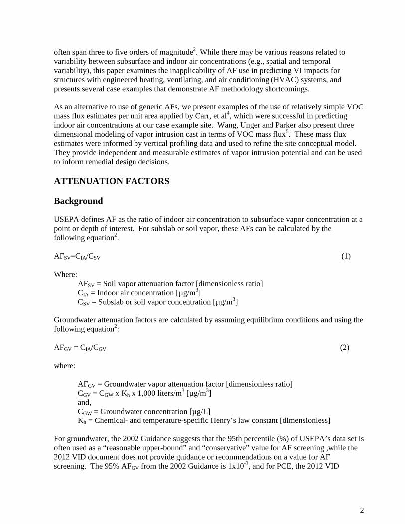
Use of VOC Mass Flux to Estimate Vapor Intrusion Impacts Paper #16 Bradley A. Green, P.G., David Shea, P.E., Andrew E. Ashton Sanborn, Head & Associates, Inc., 20 Foundry Street, Concord, NH 03301 ABSTRACT Estimating the potential impacts of volatile organic compound (VOC) vapor intrusion into buildings often relies on the use of prescribed, generic concentration ratios between indoor air and subsurface media, commonly referred to as “attenuation factors.” The use of prescribed attenuation factors, which are lumped, unitless parameters, fails to account for site-specific mass transfer processes that are ultimately responsible for realizing vapor intrusion. This paper will show how site-specific estimates of mass flux can improve vapor intrusion assessments. Because mass flux better reflects actual mass transfer processes, its use can help identify and enhance understanding of sites that pose vapor intrusion risks. Through several project examples, we will show how generic attenuation factors developed primarily based on data from residential structures can be misleading in evaluating vapor intrusion, particularly for large buildings equipped with HVAC air handling units. As an alternative approach, several direct and indirect methods to estimate mass flux will be illustrated to help support vapor intrusion evaluations. Methods to be discussed will include: i) estimating mass transfer across the vadose and shallow saturated zone supported by vertical profiling, ii) estimating diffusive flux through the building floor slab based on subslab gas concentrations, and iii) using HVAC system data to estimate mass flux though the building envelope via the combination of advection and diffusion. These methods can provide independent, quantitative estimates of mass flux that offer multiple lines of evidence for evaluating vapor intrusion and the potential magnitude of impacts to indoor air quality. Finally, we will also demonstrate how the use of mass flux estimates can support the design and implementation of efficient mitigation strategies. INTRODUCTION Generic attenuation factors (AFs) are often used to estimate the vapor intrusion potential and prediction of risk to receptors within a building due to underlying volatile organic compound (VOC) contamination. These AFs are empirically derived concentration ratios between indoor air and paired subsurface media (e.g., soil gas or groundwater) sample locations obtained from publically available data sets that consist of data from primarily residential structures, most notably the Unites States Environmental Protection Agency’s (USEPA’s) 2002 Vapor Intrusion Guidance Document1 and more recently, USEPA’s 2012 Vapor Intrusion Database (VID)2. AFs are often used in a predictive manner, particularly in the initial screening process, to make decisions about whether subsurface VOC concentrations are sufficiently high to engender unacceptable indoor air concentrations and thus warrant further investigation or remedial action3. The multi-site paired indoor air and subsurface data from USEPA’s documents that are the basis for the AFs demonstrate that for a given subsurface concentration, indoor air concentrations

2

often span three to five orders of magnitude2. While there may be various reasons related to variability between subsurface and indoor air concentrations (e.g., spatial and temporal variability), this paper examines the inapplicability of AF use in predicting VI impacts for structures with engineered heating, ventilating, and air conditioning (HVAC) systems, and presents several case examples that demonstrate AF methodology shortcomings. As an alternative to use of generic AFs, we present examples of the use of relatively simple VOC mass flux estimates per unit area applied by Carr, et al4, which were successful in predicting indoor air concentrations at our case example site. Wang, Unger and Parker also present three dimensional modeling of vapor intrusion cast in terms of VOC mass flux5. These mass flux estimates were informed by vertical profiling data and used to refine the site conceptual model. They provide independent and measurable estimates of vapor intrusion potential and can be used to inform remedial design decisions. ATTENUATION FACTORS Background USEPA defines AF as the ratio of indoor air concentration to subsurface vapor concentration at a point or depth of interest. For subslab or soil vapor, these AFs can be calculated by the following equation2. AFSV=CIA/CSV (1) Where:

AFSV = Soil vapor attenuation factor [dimensionless ratio] CIA = Indoor air concentration [µg/m3] CSV = Subslab or soil vapor concentration [µg/m3]

Groundwater attenuation factors are calculated by assuming equilibrium conditions and using the following equation2: AFGV = CIA/CGV (2) where:

AFGV = Groundwater vapor attenuation factor [dimensionless ratio] CGV = CGW x Kh x 1,000 liters/m3 [µg/m3] and, CGW = Groundwater concentration [µg/L] Kh = Chemical- and temperature-specific Henry’s law constant [dimensionless]

For groundwater, the 2002 Guidance suggests that the 95th percentile (%) of USEPA’s data set is often used as a “reasonable upper-bound” and “conservative” value for AF screening ,while the 2012 VID document does not provide guidance or recommendations on a value for AF screening. The 95% AFGV from the 2002 Guidance is 1x10-3, and for PCE, the 2012 VID

3

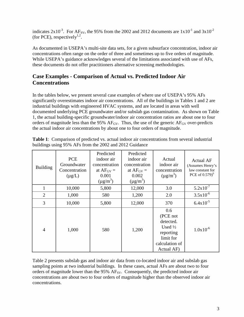
indicates 2x10-3. For AFSV, the 95% from the 2002 and 2012 documents are 1x10-1 and 3x10-2 (for PCE), respectively1,2. As documented in USEPA’s multi-site data sets, for a given subsurface concentration, indoor air concentrations often range on the order of three and sometimes up to five orders of magnitude. While USEPA’s guidance acknowledges several of the limitations associated with use of AFs, these documents do not offer practitioners alternative screening methodologies. Case Examples - Comparison of Actual vs. Predicted Indoor Air Concentrations In the tables below, we present several case examples of where use of USEPA’s 95% AFs significantly overestimates indoor air concentrations. All of the buildings in Tables 1 and 2 are industrial buildings with engineered HVAC systems, and are located in areas with well documented underlying PCE groundwater and/or subslab gas contamination. As shown on Table 1, the actual building-specific groundwater/indoor air concentration ratios are about one to four orders of magnitude less than the 95% AFGV. Thus, the use of the generic AFGV over-predicts the actual indoor air concentrations by about one to four orders of magnitude. Table 1: Comparison of predicted vs. actual indoor air concentrations from several industrial buildings using 95% AFs from the 2002 and 2012 Guidance

Building

PCE Groundwater Concentration

(µg/L)

Predicted indoor air

concentration at AFGV =

0.001 (µg/m3)

Predicted indoor air

concentration at AFGV =

0.002 (µg/m3)

Actual indoor air

concentration (µg/m3)

Actual AF (Assumes Henry’s law constant for PCE of 0.579)6

1 10,000 5,800 12,000 3.0 5.2x10-7 2 1,000 580 1,200 2.0 3.5x10-6

3 10,000 5,800 12,000 370 6.4x10-5

4 1,000 580 1,200

0.6 (PCE not detected. Used ½

reporting limit for

calculation of Actual AF)

1.0x10-6

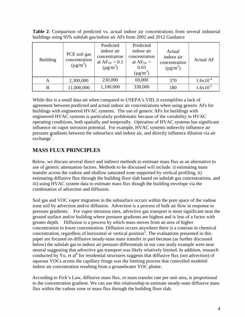
Table 2 presents subslab gas and indoor air data from co-located indoor air and subslab gas sampling points at two industrial buildings. In these cases, actual AFs are about two to four orders of magnitude lower than the 95% AFSV. Consequently, the predicted indoor air concentrations are about two to four orders of magnitude higher than the observed indoor air concentrations.

4

Table 2: Comparison of predicted vs. actual indoor air concentrations from several industrial buildings using 95% subslab gas/indoor air AFs from 2002 and 2012 Guidance

Building PCE soil gas concentration

(µg/m3)

Predicted indoor air

concentration at AFSV = 0.1

(µg/m3)

Predicted indoor air

concentration at AFSV =

0.03 (µg/m3)

Actual indoor air

concentration (µg/m3)

Actual AF

A 2,300,000 230,000 69,000 370 1.6x10-4 B 11,000,000 1,100,000 330,000 180 1.6x10-5

While this is a small data set when compared to USEPA’s VID, it exemplifies a lack of agreement between predicted and actual indoor air concentrations when using generic AFs for buildings with engineered HVAC systems. The use of generic AFs for buildings with engineered HVAC systems is particularly problematic because of the variability in HVAC operating conditions, both spatially and temporally. Operation of HVAC systems has significant influence on vapor intrusion potential. For example, HVAC systems indirectly influence air pressure gradients between the subsurface and indoor air, and directly influence dilution via air exchange7. MASS FLUX PRINCIPLES Below, we discuss several direct and indirect methods to estimate mass flux as an alternative to use of generic attenuation factors. Methods to be discussed will include: i) estimating mass transfer across the vadose and shallow saturated zone supported by vertical profiling, ii) estimating diffusive flux through the building floor slab based on subslab gas concentrations, and iii) using HVAC system data to estimate mass flux though the building envelope via the combination of advection and diffusion. Soil gas and VOC vapor migration in the subsurface occurs within the pore space of the vadose zone soil by advection and/or diffusion. Advection is a process of bulk air flow in response to pressure gradients. For vapor intrusion sites, advective gas transport is most significant near the ground surface and/or building where pressure gradients are highest and is less of a factor with greater depth. Diffusion is a process by which mass moves from an area of higher concentration to lower concentration. Diffusion occurs anywhere there is a contrast in chemical concentration, regardless of horizontal or vertical position2. The evaluations presented in this paper are focused on diffusive steady-state mass transfer in part because (as further discussed below) the subslab gas to indoor air pressure differentials in our case study example were near neutral suggesting that advective gas transport was likely relatively limited. In addition, research conducted by Yu, et al6 for residential structures suggests that diffusive flux (not advection) of aqueous VOCs across the capillary fringe was the limiting process that controlled modeled indoor air concentration resulting from a groundwater VOC plume. According to Fick’s Law, diffusive mass flux, or mass transfer rate per unit area, is proportional to the concentration gradient. We can use this relationship to estimate steady-state diffusive mass flux within the vadose zone or mass flux through the building floor slab.

5

Mass flux, J is approximated by: 𝐽 [𝜇𝑔 𝑚2 ℎ𝑟⁄⁄ ] = 𝐷𝑒

𝑑𝑐𝑑𝑧

(3) where: 𝑑𝑐𝑑𝑧

= concentration gradient [µg/m³/m] 𝐷𝑒 = effective diffusion coefficient of chemical through the subsurface [m²/hr]

𝐷𝑒 = 𝐷𝑎𝑖𝑟×(𝜃𝑎)3.33

(𝜃𝑇)2 + �𝐷𝑤𝑎𝑡𝑒𝑟𝐾ℎ

� �𝜃𝑤3.33

(𝜃𝑇)2� (4)

and,

𝐷𝑎𝑖𝑟 = free air diffusion coefficient for chemical of concern [𝑐𝑚2 ℎ𝑟⁄ ] 𝐷𝑤𝑎𝑡𝑒𝑟 = free water diffusion coefficient for chemical of concern [𝑐𝑚2 ℎ𝑟⁄ ] 𝜃𝑇 = Total porosity (unitless fraction) 𝜃𝑎 = Air-filled porosity (unitless fraction) 𝜃𝑤 = Water-filled porosity(unitless fraction) 𝐾ℎ = Henry’s constant (unitless ratio)

As can be seen from equation 4, diffusion of VOCs in the vadose zone is strongly influenced by soil moisture content. All other things being equal, as the percentage of water-filled void space decrease, and the portion of void space filled with air increases, the importance of diffusion increases. Consequently, relatively dry soils are conducive to advective and diffusive transport of VOCs; whereas, relatively wet soils are not. Therefore, understanding soil texture and moisture content is useful in assessing vapor intrusion potential. Further, understanding chemical concentrations and phase transfer processes within the vadose zone in soil, soil vapor, or pore water, as well as underlying groundwater, is also important to understanding transport of VOCs and ultimately in assessing subsurface mass flux. For buildings where air exchange rates can be directly measured, we can also evaluate mass flux by use of the following equation. Under steady-state conditions for a given room volume, the mass entering through the floor slab is equal to the mass exiting via the HVAC system (assuming no leakage), and 𝐽 𝑥 𝐴 = 𝐶𝑖𝑛𝑑𝑜𝑜𝑟 𝑥 𝑉 𝑥 (𝑄 𝑉⁄ ) (5) where: Cindoor = Concentration in indoor air [µg/m³] A = area of building footprint [m2] V = Volume of the building [m3] Q = Air exchange through the building space [m3/hr] Substituting for V

6

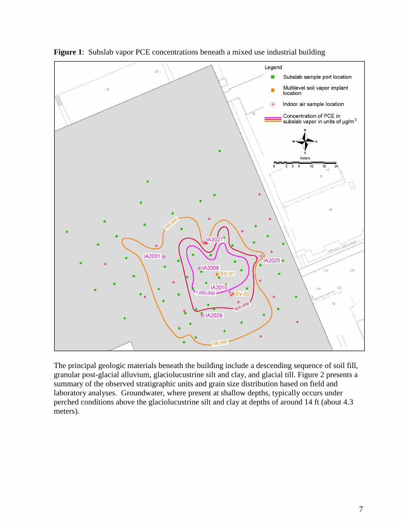
𝑉 = 𝐴 𝑥 𝐻 (6) where: H = Building height [m] and (𝑄/𝑉) = 𝐴𝐶𝐻 (𝑎𝑖𝑟 𝑐ℎ𝑎𝑛𝑔𝑒𝑠 𝑝𝑒𝑟 ℎ𝑜𝑢𝑟) (7) Then equation (5) becomes 𝐽 = 𝐶𝑖𝑛𝑑𝑜𝑜𝑟 𝑥 𝐻 𝑥 𝐴𝐶𝐻 (8) Upon rearranging this equation, we have a relationship to predict indoor air concentration from mass flux: 𝐶𝑖𝑛𝑑𝑜𝑜𝑟 = 𝐽/(𝐻 𝑥 𝐴𝐶𝐻) (9) CASE EXAMPLE OF MASS FLUX ASSESSMENT WITH SUPPORTING VADOSE ZONE PROFILING Background An approximately 30,000 square meter (m2) mixed use industrial building overlies VOC-contaminated groundwater, soil, and soil vapor (primarily PCE), which has engendered elevated concentrations of PCE in indoor air with near neutral pressure differentials between subslab gas and indoor air. We installed and collected VOC samples from approximately 90 subslab vapor ports. As shown on Figure 1, subslab VOC concentrations greater than or equal to 100,000 µg/m3 encompass an area of approximately 2,800 m2. This elevated subslab VOC presence is co-located with the area of highest observed indoor air concentrations. The area of highest subslab PCE concentrations was the focus of additional vertical profiling for further characterization of the vadose zone. Additional investigations included advancing and logging of soil borings, along with the collection of soil samples for laboratory analysis of VOCs, gradation analysis, and moisture content. We installed and sampled subslab vapor implants and multi-depth soil vapor and/or groundwater monitoring devices and submitted soil vapor and groundwater samples for laboratory analysis of VOCs. We recorded multiple rounds of air pressure differentials between subslab gas and indoor air. We also measured the flow rates of the outside air supply from each of the HVAC air handling units (AHUs) that served this portion of the building.

7

Figure 1: Subslab vapor PCE concentrations beneath a mixed use industrial building

The principal geologic materials beneath the building include a descending sequence of soil fill, granular post-glacial alluvium, glaciolucustrine silt and clay, and glacial till. Figure 2 presents a summary of the observed stratigraphic units and grain size distribution based on field and laboratory analyses. Groundwater, where present at shallow depths, typically occurs under perched conditions above the glaciolucustrine silt and clay at depths of around 14 ft (about 4.3 meters).

8

Figure 2: Summary of observed stratigraphic units

Soil fill ƟT=0.3 Ɵa=0.24 Ɵw=0.06

Post-glacial Alluvial soils ƟT=0.3 Ɵa=0.24 Ɵw=0.06

Glacio-lucustrine silt/clay ƟT=0.5 Ɵa=0.02 Ɵw=0.48 Glacial Till ƟT=0.35 Ɵa=0.13 Ɵw=0.22

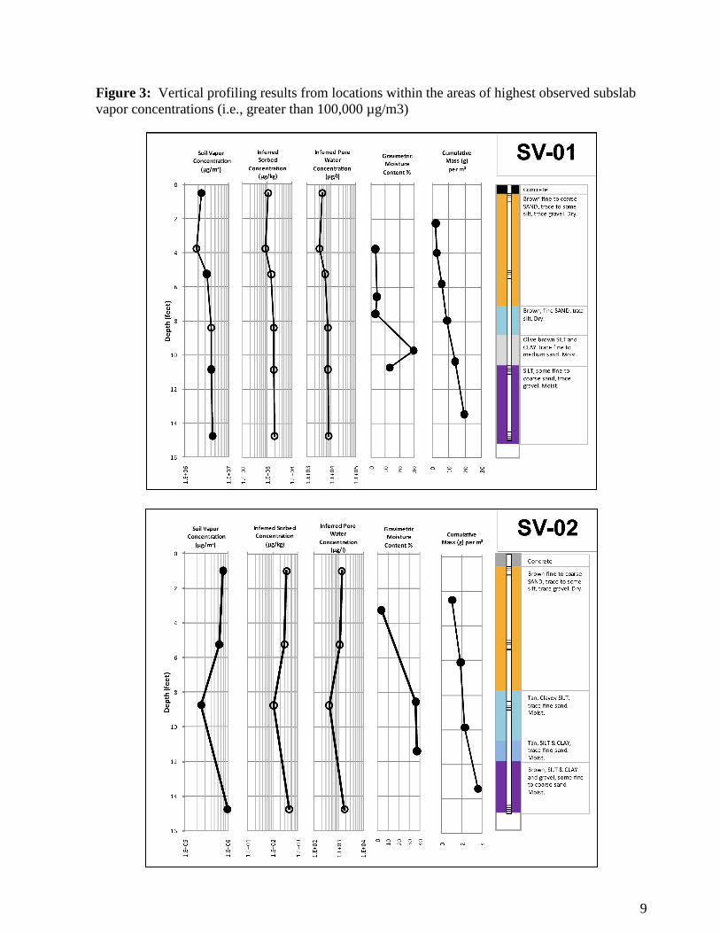
Vertical profiling was focused on assessing the influence of subsurface conditions on the flux of VOCs in the subsurface. We collected samples to assess grain size; moisture content; and PCE concentrations in soil, soil vapor, and groundwater. Typical soil moisture conditions and porosities within each stratigraphic unit are presented on Figure 2. Measured PCE soil vapor concentration, inferred sorbed soil PCE concentration, and measured or inferred pore water concentrations from two multi-level sampling locations within the area exhibiting subslab PCE concentrations greater than 100,000 µg/m3 are presented on Figure 3.

9

Figure 3: Vertical profiling results from locations within the areas of highest observed subslab vapor concentrations (i.e., greater than 100,000 µg/m3)

10

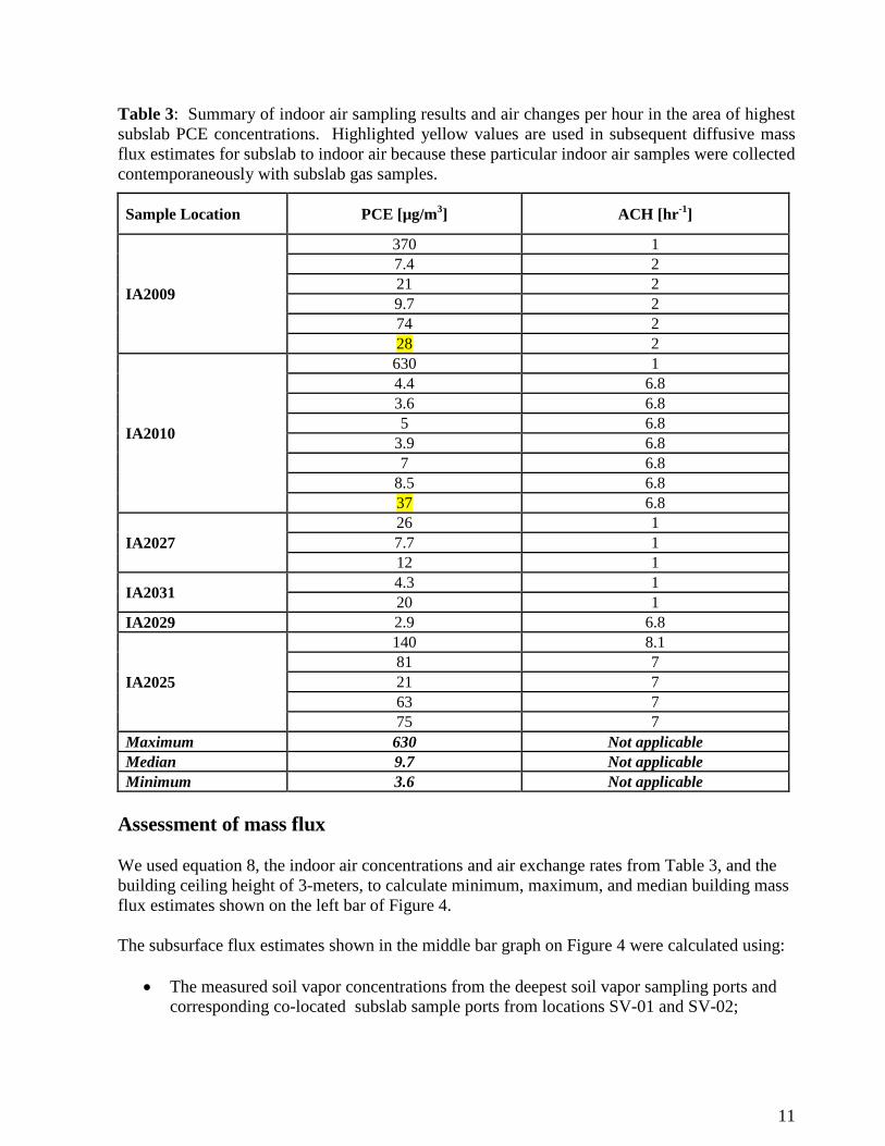
As summarized in Figure 3, soil vapor and soil PCE concentrations decline by less than an order of magnitude with depth, consistent with small concentration gradients driving diffusion across dry soils capped by the concrete floor of the building. The small gradients and modest “attenuation” of VOC concentrations is consistent with mature conditions decades after the original solvent release, and where PCE-containing groundwater or soil may be present in underlying silt/clay or glacial till soil. This subsurface PCE presence has resulted in the presence of PCE in indoor air as further summarized below. Soil moisture conditions in the fill and alluvial soils are relatively low (see Figure 2), which could, in theory, suggest that advection would be an important transport mechanism. However, as described above, the subslab to indoor air pressure differentials were near neutral which leads us to believe that diffusion is a more important transport mechanism than advection in our case example. Approximately 27 indoor air samples were collected at various times from six locations within the area with subslab PCE concentrations greater than 100,000 µg/m3. Indoor air PCE concentrations and measured air changes per hour (ACH) are presented in Table 3.

11

Table 3: Summary of indoor air sampling results and air changes per hour in the area of highest subslab PCE concentrations. Highlighted yellow values are used in subsequent diffusive mass flux estimates for subslab to indoor air because these particular indoor air samples were collected contemporaneously with subslab gas samples.

Sample Location PCE [µg/m3] ACH [hr-1]

IA2009

370 1 7.4 2 21 2 9.7 2 74 2 28 2

IA2010

630 1 4.4 6.8 3.6 6.8 5 6.8

3.9 6.8 7 6.8

8.5 6.8 37 6.8

IA2027 26 1 7.7 1 12 1

IA2031 4.3 1 20 1

IA2029 2.9 6.8

IA2025

140 8.1 81 7 21 7 63 7 75 7

Maximum 630 Not applicable Median 9.7 Not applicable Minimum 3.6 Not applicable

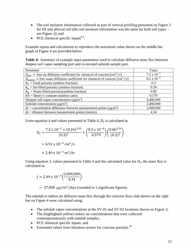
Assessment of mass flux We used equation 8, the indoor air concentrations and air exchange rates from Table 3, and the building ceiling height of 3-meters, to calculate minimum, maximum, and median building mass flux estimates shown on the left bar of Figure 4. The subsurface flux estimates shown in the middle bar graph on Figure 4 were calculated using:

• The measured soil vapor concentrations from the deepest soil vapor sampling ports and corresponding co-located subslab sample ports from locations SV-01 and SV-02;

12

• The soil moisture information collected as part of vertical profiling presented on Figure 2 for fill and alluvial soil (the soil moisture information was the same for both soil types – see Figure 2); and

• PCE chemical specific inputs8,9. Example inputs and calculations to reproduce the maximum value shown on the middle bar graph of Figure 4 are provided below: Table 4: Summary of example input parameters used to calculate diffusive mass flux between deepest soil vapor sampling port and co-located subslab sample port. Parameter Value 𝐷𝑎𝑖𝑟 = free air diffusion coefficient for chemical of concern [𝑐𝑚2 𝑠⁄ ] 7.2 x 10 -2 𝐷𝑤𝑎𝑡𝑒𝑟 = free water diffusion coefficient for chemical of concern [𝑐𝑚2 𝑠⁄ ] 8.2 x 10 -6 𝜃𝑇 = Total porosity (unitless fraction) 0.3 𝜃𝑎 = Air-filled porosity (unitless fraction) 0.24 𝜃𝑤 = Water-filled porosity(unitless fraction) 0.06 𝐾ℎ = Henry’s constant (unitless ratio) 0.579 Deepest soil vapor concentration (µg/m3) 4,400,000 Subslab concentration (µg/m3) 2,400,000 dc = concentration difference between measurement points (µg/m3) 2,000,000 dz = distance between measurement points (meters) 4.34 From equation 4 and values presented in Table 4, De is calculated as

𝐷𝑒 =7.2 x 10−2 × (0.24)3.33

(0.3)2 + �8.2 x 10−6

0.579��

0.063.33

(0.3)2�

= 6.91 x 10−3 𝑐𝑚2/𝑠 = 2.49 x 10−3 𝑚2/ℎ𝑟

Using equation 3, values presented in Table 4 and the calculated value for De, the mass flux is calculated as

𝐽 = 2.49 x 10−3 �2,000,000

4.34�

= 27,000 𝜇𝑔 𝑚2 𝑑𝑎𝑦⁄⁄ (rounded to 2 significant figures).

The subslab to indoor air diffusive mass flux through the concrete floor slab shown on the right bar on Figure 4 were calculated using:

• The subslab vapor concentrations at the SV-01 and SV-02 locations shown on Figure 3; • The (highlighted yellow) indoor air concentrations that were collected

contemporaneously with subslab samples; • PCE chemical specific inputs; and • Estimated values from literature review for concrete porosity.10

13

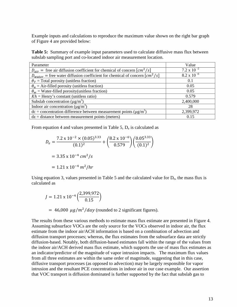
Example inputs and calculations to reproduce the maximum value shown on the right bar graph of Figure 4 are provided below: Table 5: Summary of example input parameters used to calculate diffusive mass flux between subslab sampling port and co-located indoor air measurement location. Parameter Value 𝐷𝑎𝑖𝑟 = free air diffusion coefficient for chemical of concern [𝑐𝑚2 𝑠⁄ ] 7.2 x 10 -2 𝐷𝑤𝑎𝑡𝑒𝑟 = free water diffusion coefficient for chemical of concern [𝑐𝑚2 𝑠⁄ ] 8.2 x 10 -6 𝜃𝑇 = Total porosity (unitless fraction) 0.1 𝜃𝑎 = Air-filled porosity (unitless fraction) 0.05 𝜃𝑤 = Water-filled porosity(unitless fraction) 0.05 𝐾ℎ = Henry’s constant (unitless ratio) 0.579 Subslab concentration (µg/m3) 2,400,000 Indoor air concentration (µg/m3) 28 dc = concentration difference between measurement points (µg/m3) 2,399,972 dz = distance between measurement points (meters) 0.15 From equation 4 and values presented in Table 5, De is calculated as

𝐷𝑒 =7.2 x 10−2 × (0.05)3.33

(0.1)2 + �8.2 x 10−6

0.579��

0.053.33

(0.1)2�

= 3.35 x 10−4 𝑐𝑚2/𝑠 = 1.21 x 10−4 𝑚2/ℎ𝑟

Using equation 3, values presented in Table 5 and the calculated value for De, the mass flux is calculated as

𝐽 = 1.21 x 10−4 �2,399,972

0.15�

= 46,000 𝜇𝑔 𝑚2 𝑑𝑎𝑦⁄⁄ (rounded to 2 significant figures).

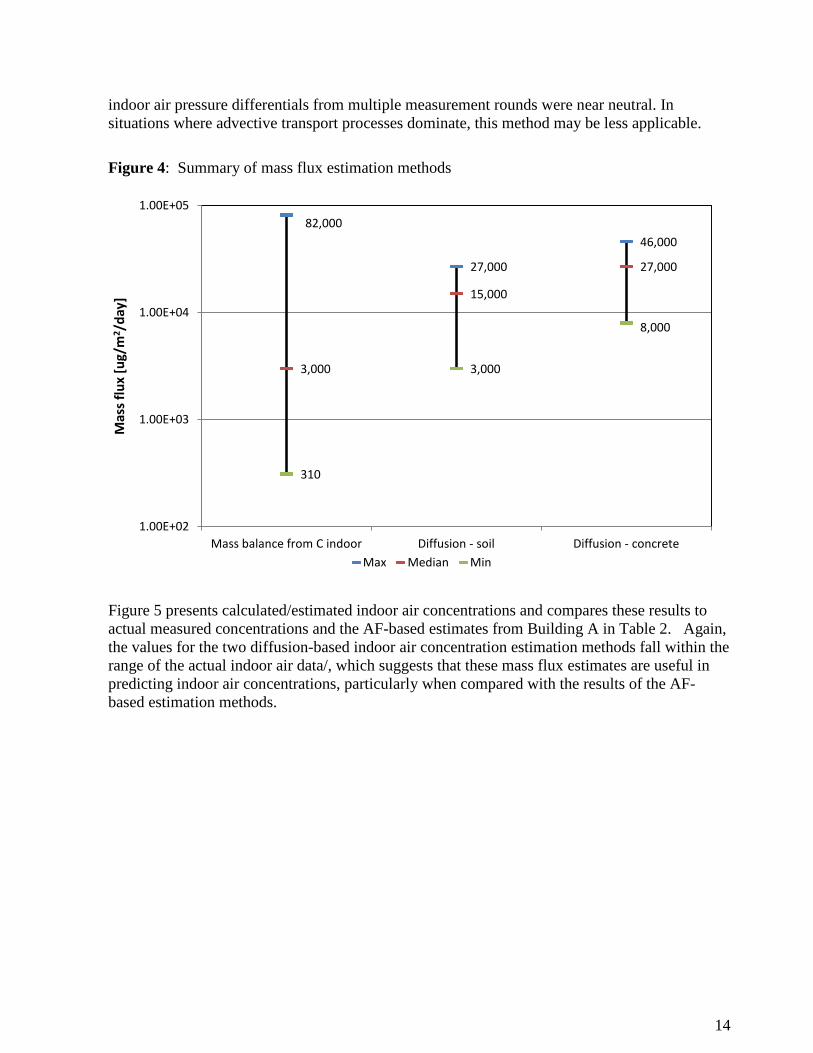
The results from these various methods to estimate mass flux estimate are presented in Figure 4. Assuming subsurface VOCs are the only source for the VOCs observed in indoor air, the flux estimate from the indoor air/ACH information is based on a combination of advection and diffusion transport processes; whereas, the flux estimates from the subsurface data are strictly diffusion-based. Notably, both diffusion-based estimates fall within the range of the values from the indoor air/ACH derived mass flux estimate, which supports the use of mass flux estimates as an indicator/predictor of the magnitude of vapor intrusion impacts. The maximum flux values from all three estimates are within the same order of magnitude, suggesting that in this case, diffusive transport processes (as opposed to advection) may be largely responsible for vapor intrusion and the resultant PCE concentrations in indoor air in our case example. Our assertion that VOC transport is diffusion dominated is further supported by the fact that subslab gas to

14

indoor air pressure differentials from multiple measurement rounds were near neutral. In situations where advective transport processes dominate, this method may be less applicable. Figure 4: Summary of mass flux estimation methods

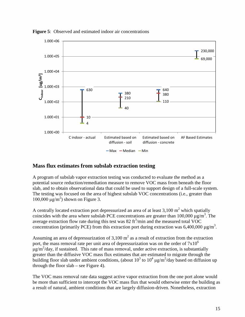
Figure 5 presents calculated/estimated indoor air concentrations and compares these results to actual measured concentrations and the AF-based estimates from Building A in Table 2. Again, the values for the two diffusion-based indoor air concentration estimation methods fall within the range of the actual indoor air data/, which suggests that these mass flux estimates are useful in predicting indoor air concentrations, particularly when compared with the results of the AF-based estimation methods.

82,000

27,000

46,000

3,000

15,000

27,000

310

3,000

8,000

1.00E+02

1.00E+03

1.00E+04

1.00E+05

Mass balance from C indoor Diffusion - soil Diffusion - concrete

Mas

s flu

x [u

g/m

2 /da

y]

Max Median Min

15

Figure 5: Observed and estimated indoor air concentrations

Mass flux estimates from subslab extraction testing A program of subslab vapor extraction testing was conducted to evaluate the method as a potential source reduction/remediation measure to remove VOC mass from beneath the floor slab, and to obtain observational data that could be used to support design of a full-scale system. The testing was focused on the area of highest subslab VOC concentrations (i.e., greater than 100,000 μg/m2) shown on Figure 3. A centrally located extraction port depressurized an area of at least 3,100 m2 which spatially coincides with the area where subslab PCE concentrations are greater than 100,000 µg/m3. The average extraction flow rate during this test was 82 ft3/min and the measured total VOC concentration (primarily PCE) from this extraction port during extraction was 6,400,000 µg/m3. Assuming an area of depressurization of 3,100 m2 as a result of extraction from the extraction port, the mass removal rate per unit area of depressurization was on the order of 7x106 μg/m2/day, if sustained. This rate of mass removal, under active extraction, is substantially greater than the diffusive VOC mass flux estimates that are estimated to migrate through the building floor slab under ambient conditions, (about 103 to 104 μg/m2/day based on diffusion up through the floor slab – see Figure 4). The VOC mass removal rate data suggest active vapor extraction from the one port alone would be more than sufficient to intercept the VOC mass flux that would otherwise enter the building as a result of natural, ambient conditions that are largely diffusion-driven. Nonetheless, extraction

630 380

640

230,000

10

210 380

4

40

110

69,000

1.00E+00

1.00E+01

1.00E+02

1.00E+03

1.00E+04

1.00E+05

1.00E+06

C indoor - actual Estimated based on diffusion - soil

Estimated based on diffusion - concrete

AF Based Estimates

C ind

oor

[ug/

m3 ]

Max Median Min

16

from more ports would promote greater rates of pore volume exchange for mass removal and provide operating flexibility for optimization and adjustment of the subslab depressurization field. SUMMARY Industry practice for vapor intrusion investigations since USEPA’s issuance of its 2002 Guidance Document has largely been focused on the use of AFs. The data used to develop AF statistics is based largely on data collected from residential homes as opposed to commercial/industrial buildings with engineered HVAC systems where the building air exchange may vary spatially by HVAC zones and temporally through modulated changes in HVAC system operation. The variability in air pressure gradients and air exchange rates fundamentally changes the vapor intrusion potential in these buildings when compared to residential structures. In addition, commercial/industrial buildings with HVAC systems typically offer greater volume and active means for indoor air mixing compared to residential structures. In this case, AFs over predict vapor intrusion potential for commercial and industrial buildings with engineered HVAC systems. In the examples presented above, predicted indoor air concentrations via the use of AFs were about two to four orders of magnitude greater than measured concentrations. The mass flux estimation methods summarized in this paper inherently include site-specific mass transfer processes and are therefore useful in predicting indoor air concentrations. Use of various mass flux estimation methods provides measurable and independent lines of evidence for assessing vapor intrusion potential. The diffusive flux estimates and associated indoor air predictions presented in this paper compared favorably with measured indoor air concentrations, typically within one order of magnitude or less. When flux estimates are informed with subsurface vertical profiling data and measured indoor air exchange rates, site conceptual models of VOC mass transfer processes are improved and mass flux estimates can be used as a predictive tool. Further, as presented in our case example, flux assessments can be compared to VOC mass removal rates developed as part of subslab extraction testing to inform and optimize final design of subslab extraction systems. As described in the body of this paper, the diffusion-based mass flux estimates were helpful in these case examples in part because advective transport is unlikely to be a significant driver of the resultant indoor air concentrations. Where advective processes more appreciably influence vapor intrusion (e.g., high subslab to indoor air pressure differentials, floor penetrations), the utility of the subsurface diffusive mass flux estimates to predict indoor air concentrations may be limited.

17

REFERENCES

1. United States Environmental Protection Agency (USEPA), OSWER Draft Guidance for Evaluating the Vapor Intrusion to Indoor Air Pathway from Groundwater and Soils (Subsurface Vapor Intrusion Guidance), November 2002.

2. USEPA, EPA’s Vapor Intrusion Database: Evaluation and Characterization of Attenuation Factors for Chlorinated Volatile Organic Compounds and Residential Buildings, March 2012.

3. California Environmental Protection Agency, Final Guidance for the Evaluation and Mitigation of Subsurface Vapor Intrusion to indoor Air (Vapor Intrusion Guidance), October 2011.

4. Carr, D.B., Shea, D. Field Evidence Scaling VOC Mass Flux at Vapor Intrusion Sites, Battelle Conference, Remediation of Chlorinated and Recalcitrant Compounds, Monterey, California, May 2012.

5. Wang, Xiaomin, Unger, A. J. A, and Parker, B. Simulating Factors Contributing to an Exclusion Zone for Vapor Intrusion of TCE from Groundwater Into Indoor Air. Under Review Journal of Contaminant Hydrology.

6. Yu, S., Unger, A.J., and Parker, B., April 2009, Simulating the Fate and Transport of TCE from Groundwater to Indoor Air,

7. Shea, D., and Carr, D.B., Vapor Intrusion into Large Buildings, USEPA Workshop: Recent Advances to VI Application and Implementation-A State of the Science Update, The 22nd Annual International Conference on Soil, Water, Energy, and Air, San Diego, California, March 2012.

Journal of Contaminant Hydrology 107 (2009) 140-161.

8. EPA On-line Tools for Site Assessment Calculation. http://www.epa.gov/athens/learn2model/part-two/onsite/esthenry.html, OSWER Method at 20 oC.

9. Air emissions models for waste and wastewater EPA-453/R-94-080A – 1994 http://www.epa.gov/ttn/chief/software/water/air_emission_models_waste_wastewater.pdf

10. Lamond, J.F. Significance of Tests and Properties of Concrete and Concrete-Making Materials, Issue 169, Part 4, ASTM International, 2006.