Use of thermal sieve to allow optical testing of cryogenic ... · PDF fileThe main function of a Thermal Sieve is ... passes through the 1st plate holes. The collimator and optical

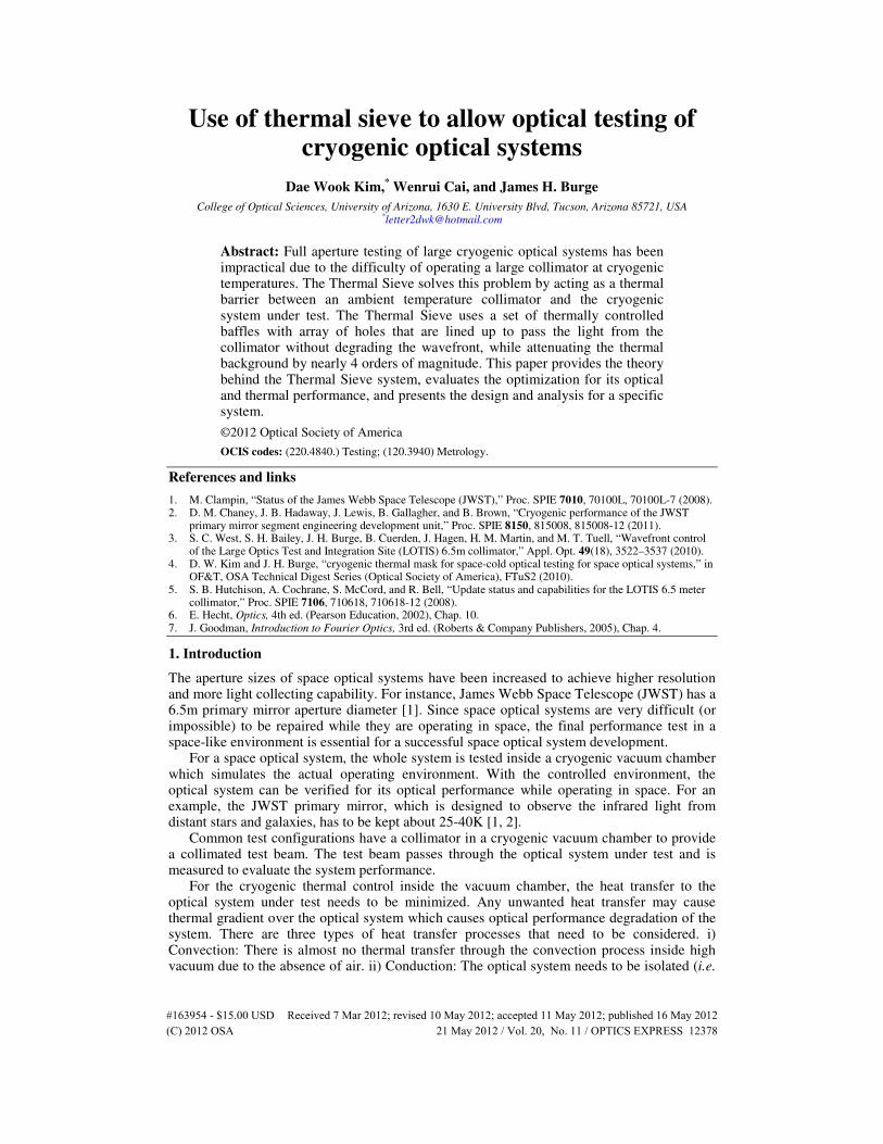
Use of thermal sieve to allow optical testing of cryogenic optical systems

Dae Wook Kim,* Wenrui Cai, and James H. Burge

College of Optical Sciences, University of Arizona, 1630 E. University Blvd, Tucson, Arizona 85721, USA *[email protected]

Abstract: Full aperture testing of large cryogenic optical systems has been impractical due to the difficulty of operating a large collimator at cryogenic temperatures. The Thermal Sieve solves this problem by acting as a thermal barrier between an ambient temperature collimator and the cryogenic system under test. The Thermal Sieve uses a set of thermally controlled baffles with array of holes that are lined up to pass the light from the collimator without degrading the wavefront, while attenuating the thermal background by nearly 4 orders of magnitude. This paper provides the theory behind the Thermal Sieve system, evaluates the optimization for its optical and thermal performance, and presents the design and analysis for a specific system.

©2012 Optical Society of America

OCIS codes: (220.4840.) Testing; (120.3940) Metrology.

References and links

1. M. Clampin, “Status of the James Webb Space Telescope (JWST),” Proc. SPIE 7010, 70100L, 70100L-7 (2008). 2. D. M. Chaney, J. B. Hadaway, J. Lewis, B. Gallagher, and B. Brown, “Cryogenic performance of the JWST

primary mirror segment engineering development unit,” Proc. SPIE 8150, 815008, 815008-12 (2011). 3. S. C. West, S. H. Bailey, J. H. Burge, B. Cuerden, J. Hagen, H. M. Martin, and M. T. Tuell, “Wavefront control

of the Large Optics Test and Integration Site (LOTIS) 6.5m collimator,” Appl. Opt. 49(18), 3522–3537 (2010). 4. D. W. Kim and J. H. Burge, “cryogenic thermal mask for space-cold optical testing for space optical systems,” in

OF&T, OSA Technical Digest Series (Optical Society of America), FTuS2 (2010). 5. S. B. Hutchison, A. Cochrane, S. McCord, and R. Bell, “Update status and capabilities for the LOTIS 6.5 meter

collimator,” Proc. SPIE 7106, 710618, 710618-12 (2008). 6. E. Hecht, Optics, 4th ed. (Pearson Education, 2002), Chap. 10. 7. J. Goodman, Introduction to Fourier Optics, 3rd ed. (Roberts & Company Publishers, 2005), Chap. 4.

1. Introduction

The aperture sizes of space optical systems have been increased to achieve higher resolution and more light collecting capability. For instance, James Webb Space Telescope (JWST) has a 6.5m primary mirror aperture diameter [1]. Since space optical systems are very difficult (or impossible) to be repaired while they are operating in space, the final performance test in a space-like environment is essential for a successful space optical system development.

For a space optical system, the whole system is tested inside a cryogenic vacuum chamber which simulates the actual operating environment. With the controlled environment, the optical system can be verified for its optical performance while operating in space. For an example, the JWST primary mirror, which is designed to observe the infrared light from distant stars and galaxies, has to be kept about 25-40K [1, 2].

Common test configurations have a collimator in a cryogenic vacuum chamber to provide a collimated test beam. The test beam passes through the optical system under test and is measured to evaluate the system performance.

For the cryogenic thermal control inside the vacuum chamber, the heat transfer to the optical system under test needs to be minimized. Any unwanted heat transfer may cause thermal gradient over the optical system which causes optical performance degradation of the system. There are three types of heat transfer processes that need to be considered. i) Convection: There is almost no thermal transfer through the convection process inside high vacuum due to the absence of air. ii) Conduction: The optical system needs to be isolated (i.e.

#163954 - $15.00 USD Received 7 Mar 2012; revised 10 May 2012; accepted 11 May 2012; published 16 May 2012(C) 2012 OSA 21 May 2012 / Vol. 20, No. 11 / OPTICS EXPRESS 12378

no direct contact) from any heat sources. iii) Radiation: Thermal radiation from a hot object needs to be blocked before it reaches to the optical system.

Because the collimator inside the vacuum chamber directly faces the optical system, the thermal radiation from the collimator becomes a critical issue for the cryogenic thermal control. One obvious solution may be a collimator operating at the same temperature as the space optical system, so that they are at a thermal equilibrium. However, making such a customized cryogenic collimator working at a particular cryogenic (e.g. ~35K) temperature may cost a significant portion of the total project budget. Thus, it is highly desired to use an existing collimator such as LOTIS operating at an ambient temperature (e.g. ~300K) [3].

A new optical testing configuration utilizing Thermal Sieve (TS), a.k.a. cryogenic thermal mask, was developed and introduced [4]. It provides effective thermal decoupling between a cryogenic optical system under test and a collimator operating at an ambient temperature, while passing the test beam without significant degradation in its wavefront. The overall concept of the TS is given in Section 2. Some practical design issues for the TS are discussed in Section 3. Thermal and optical performance of the TS is evaluated in Section 4. The summary and future works are stated in Section 5.

2. Cryogenic optical testing using Thermal Sieve

2.1 Optical testing configuration using TS

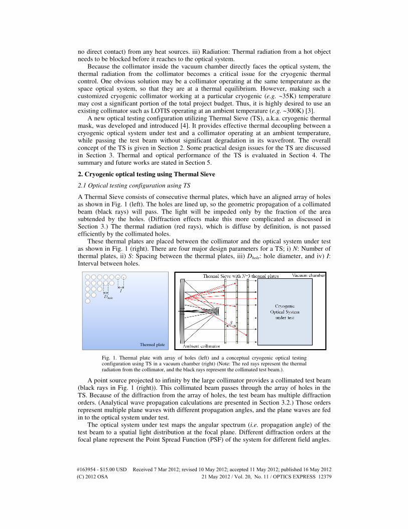
A Thermal Sieve consists of consecutive thermal plates, which have an aligned array of holes as shown in Fig. 1 (left). The holes are lined up, so the geometric propagation of a collimated beam (black rays) will pass. The light will be impeded only by the fraction of the area subtended by the holes. (Diffraction effects make this more complicated as discussed in Section 3.) The thermal radiation (red rays), which is diffuse by definition, is not passed efficiently by the collimated holes.

These thermal plates are placed between the collimator and the optical system under test as shown in Fig. 1 (right). There are four major design parameters for a TS; i) N: Number of thermal plates, ii) S: Spacing between the thermal plates, iii) Dhole: hole diameter, and iv) I: Interval between holes.

Fig. 1. Thermal plate with array of holes (left) and a conceptual cryogenic optical testing configuration using TS in a vacuum chamber (right) (Note: The red rays represent the thermal radiation from the collimator, and the black rays represent the collimated test beam.).

A point source projected to infinity by the large collimator provides a collimated test beam (black rays in Fig. 1 (right)). This collimated beam passes through the array of holes in the TS. Because of the diffraction from the array of holes, the test beam has multiple diffraction orders. (Analytical wave propagation calculations are presented in Section 3.2.) Those orders represent multiple plane waves with different propagation angles, and the plane waves are fed in to the optical system under test.

The optical system under test maps the angular spectrum (i.e. propagation angle) of the test beam to a spatial light distribution at the focal plane. Different diffraction orders at the focal plane represent the Point Spread Function (PSF) of the system for different field angles.


By evaluating the zero order (i.e. on-axis) PSF only, various optical testings (e.g. wavefront measurement, point source imaging) can be made downstream [5].

2.2 Thermal transfer control using TS

The main function of a Thermal Sieve is control of thermal transfer. The thermal transfer between the plates is limited by the emissivity of the plates and the relatively small area encompassed by the holes. This is conceptually depicted in Fig. 1 (right) as red rays, which represent the thermal radiation from the ambient collimator. The temperature of each thermal plate is independently controlled to gradually match the temperature difference between the collimator and the optical system spaces.

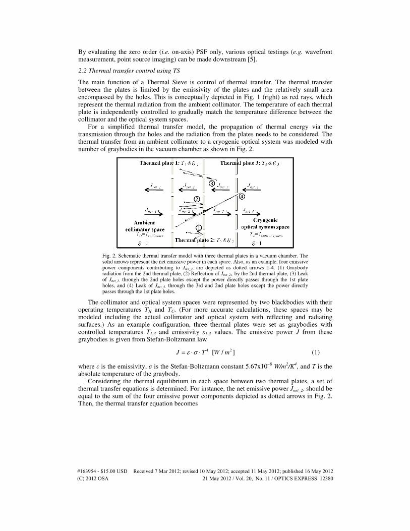
For a simplified thermal transfer model, the propagation of thermal energy via the transmission through the holes and the radiation from the plates needs to be considered. The thermal transfer from an ambient collimator to a cryogenic optical system was modeled with number of graybodies in the vacuum chamber as shown in Fig. 2.

Fig. 2. Schematic thermal transfer model with three thermal plates in a vacuum chamber. The solid arrows represent the net emissive power in each space. Also, as an example, four emissive power components contributing to Jnet_2- are depicted as dotted arrows 1-4. (1) Graybody radiation from the 2nd thermal plate, (2) Reflection of Jnet_2+ by the 2nd thermal plate, (3) Leak of Jnet_3- through the 2nd plate holes except the power directly passes through the 1st plate holes, and (4) Leak of Jnet_4- through the 3rd and 2nd plate holes except the power directly passes through the 1st plate holes.

The collimator and optical system spaces were represented by two blackbodies with their operating temperatures TH and TC. (For more accurate calculations, these spaces may be modeled including the actual collimator and optical system with reflecting and radiating surfaces.) As an example configuration, three thermal plates were set as graybodies with controlled temperatures T1-3 and emissivity ε1-3 values. The emissive power J from these graybodies is given from Stefan-Boltzmann law

4 2[ / ]J T W mε σ= ⋅ ⋅ (1)

where ε is the emissivity, σ is the Stefan-Boltzmann constant 5.67x10−8

W/m2/K

4, and T is the

absolute temperature of the graybody. Considering the thermal equilibrium in each space between two thermal plates, a set of

thermal transfer equations is determined. For instance, the net emissive power Jnet_2- should be equal to the sum of the four emissive power components depicted as dotted arrows in Fig. 2. Then, the thermal transfer equation becomes


4

_ 2 2 2

_ 2 2

1

_ 3

1 2

_ 4

: (1) .2.

(1 ) : (2) .2.

( )(1 ) : (3) .2.

( )(1 ) : (4) .2.

net

net

eff

net

eff eff

net

J T in Fig

J in Fig

J in Fig

J in Fig

ε σ α

ε α

πα

π

απ

−

+

−

−

= ⋅ ⋅ ⋅

+ ⋅ − ⋅

−Ω+ ⋅ ⋅ −

Ω −Ω+ ⋅ ⋅ −

(2)

where the obscuration ratio α of each thermal plate was defined as the ratio of the not-a-hole region area to the whole thermal plate area. Two effective solid angle Ωeff1 and Ωeff2 represent the sum of solid angles encompassed by the array of holes in the neighboring plate (S away) and the following plate (2S away), respectively. These solid angles are expressed using approximated projected solid angles with cos

4θ scale factor as

2 2

4 4

1 2 2 2 2 2 21 10 0

( / 2)(1 4 cos ) 1 4 ( )

4 ( )

hole hole

eff

n nm m

D D S

S S S I n m

π πθ

∞ ∞

= == =

⋅ ⋅Ω ≅ + = +

+ +∑ ∑ (3)

and

2 2

4 4

2 2 2 2 2 2 21 10 0

( / 2)(1 4 cos ) 1 4 ( )

(2 ) 16 ( )

hole hole

eff

n nm m

D D S

S S S I n m

π πθ

∞ ∞

= == =

⋅ ⋅Ω ≅ + = +

+ +∑ ∑ (4)

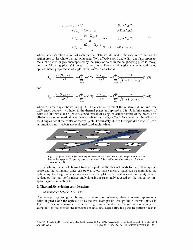
where θ is the angle shown in Fig. 3. The n and m represent the relative column and row differences between two holes in the thermal plates as depicted in Fig. 3. Infinite number of holes (i.e. infinite n and m) was assumed instead of using the actual number of the holes. This eliminates the geometrical asymmetry problem (e.g. edge effect) for evaluating the effective solid angles not at the center of thermal plate. Fortunately, due to the rapid drop of cos

4θ, this

assumption hardly affects the evaluated solid angle values.

Fig. 3. Projected solid angle geometry between a hole at the bottom thermal plate and another hole at the top plate (S: spacing between the plates, I: interval between holes) for n = 2 and m = 1 case in Eq. (3).

By solving the set of thermal transfer equations the thermal loads to the optical system space and the collimator space can be evaluated. Those thermal loads can be minimized via optimizing TS design parameters such as thermal plate’s temperatures and emissivity values. A detailed thermal performance analysis using a case study focused on the optical system space is given in Section 4.1.

3. Thermal Sieve design considerations

3.1 Independence between hole-sets

The wave propagation going through a large array of hole-sets, where a hole-set represents N holes aligned along the optical axis as the test beam passes through the N thermal plates in Fig. 1 (right), is a numerically demanding simulation due to the interaction among the complex light fields from the thousands of hole-sets. Especially, the periodic pattern needs to


be perturbed to model imperfect alignment, and it becomes almost an impossible simulation task within today’s computing power.

This entanglement issue can be ignored if each complex field is almost confined within its own hole-set while it propagates through. This independence assumption allows us to express the complex field right after passing the TS in a simple form as presented in Section 3.2. The tolerance analysis in Section 4.2 is also performed based on this assumption.

In order to accomplish this independence condition, the holes need to be large enough that the light remains mostly collimated in the region between plates. Also, the interval between holes I needs to be larger than the extent of diffraction spread in the geometrical shadow region (i.e. outside a hole). Then, most of the light can go straight through a hole-set without interacting with other holes. In other words, the diffraction spread needs to be small compared to the hole size Dhole and the interval I between the holes. (Note: I > Dhole by definition shown in Fig. 1.) Using the edge diffraction model [6], which approximates the spread from the circular aperture edge, a condition for Dhole defined in terms of wavelength λ and propagation distance S as

2 .2

hole

SD

λ ⋅> (5)

A scale factor of 2 was applied to take account the spread in both directions, and the extent of the spread was chosen where the irradiance drops down to <~5% of the nominal irradiance from the edge diffraction model [6].

These independence conditions were investigated by performing rigorous wave propagation simulations through an example hole-set using Fresnel diffraction model [7]. TS design parameters in Table 1, which satisfy Eq. (5), were used for the simulation.

Table 1. TS Design Parameter Values for a Hole-set Wave Propagation Simulation

Parameters Symbol Value

Diameter of a hole Dhole 0.002 m Interval between holes I 0.02 m Spacing between plates S 0.25 m Number of thermal plates N 3 Wavelength λ 1µm

An electric field in an x-y plane is expressed using complex field notations as

2

( , ) ( , ) exp( ( , ))U x y A x y i x yπλ

= ⋅ ⋅ ⋅Φ (6)

where A is the amplitude, Φ is the phase in waves, λ is the wavelength of the field. The actual field is the real part of this complex field. Based on the Fresnel near-field diffraction model [7] the complex field at the next thermal plate Un(xn, yn) becomes

2 2( , ) [ ( , ) exp ( )]

n nn n n y x p p p p p

S S

iU x y F F U x y x y

Sη ξλ λ

πλ= =

⋅ ⋅

⋅∝ ⋅ +

⋅ (7)

where FF represents the 2D Fourier transform, Up(xp, yp) is the complex field at the previous thermal plate, and S is the distance between thermal plates (i.e. propagation distance).

The collimated test beam was propagated through the three holes in a hole-set and evaluated after the last hole in the 3rd thermal plate. The resulting intensity distribution (i.e. squared modulus of the complex field) at each holes are presented in Fig. 4.


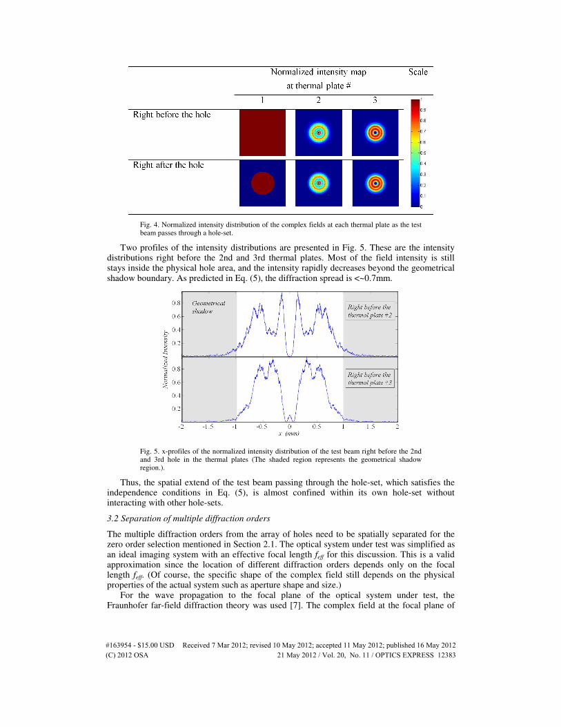
Fig. 4. Normalized intensity distribution of the complex fields at each thermal plate as the test beam passes through a hole-set.

Two profiles of the intensity distributions are presented in Fig. 5. These are the intensity distributions right before the 2nd and 3rd thermal plates. Most of the field intensity is still stays inside the physical hole area, and the intensity rapidly decreases beyond the geometrical shadow boundary. As predicted in Eq. (5), the diffraction spread is <~0.7mm.

Fig. 5. x-profiles of the normalized intensity distribution of the test beam right before the 2nd and 3rd hole in the thermal plates (The shaded region represents the geometrical shadow region.).

Thus, the spatial extend of the test beam passing through the hole-set, which satisfies the independence conditions in Eq. (5), is almost confined within its own hole-set without interacting with other hole-sets.

3.2 Separation of multiple diffraction orders

The multiple diffraction orders from the array of holes need to be spatially separated for the zero order selection mentioned in Section 2.1. The optical system under test was simplified as an ideal imaging system with an effective focal length feff for this discussion. This is a valid approximation since the location of different diffraction orders depends only on the focal length feff. (Of course, the specific shape of the complex field still depends on the physical properties of the actual system such as aperture shape and size.)

For the wave propagation to the focal plane of the optical system under test, the Fraunhofer far-field diffraction theory was used [7]. The complex field at the focal plane of


the optical system Ufocal is expressed in a 2D Fourier transform of the test beam complex field UTS as

( , ) [ ( , )]

eff eff

focal y x TS

f f

U x y F F U x yη ξ

λ λ= =

⋅ ⋅

∝ (8)

where feff is the effective focal length of the optical system under test. The complex field UTS is the complex field after passing through the TS, and can be expressed as

2 2

( , ) ( ) ( , ) ( , )TS hole

TS

x y x yU x y cyl comb U x y

D I I

+ = ⋅ ∗∗

(9)

where ** represents the 2D convolution, I is the interval between holes, DTS is the diameter of the TS circular aperture, and Uhole is the complex field in a hole at the last thermal plate. Identical complex field Uhole was assumed for all holes at the last thermal plate thanks to the independence assumption in Section 3.1, so that UTS was expressed using 2D comb function defined in Appendix A.1.

By inserting Eq. (9) to Eq. (8), the complex field at the focal plane becomes

2 2

2 2

2 2

( , ) [ ( ) ( , ) ( , )]

[ ( )]** [ ( , )** ( , )]

( ) ( ,

eff eff

eff eff eff eff

focal y x hole

TSf f

y x y x hole

TSf f f f

TS

eff eff

x y x yU x y F F cyl comb U x y

D I I

x y x yF F cyl F F comb U x y

D I I

D x y I x I ysomb comb

f f

η ξλ λ

η ξ η ξλ λ λ λ

λ λ λ

= =⋅ ⋅

= = = =⋅ ⋅ ⋅ ⋅

+∝ ⋅ ∗∗

+=

⋅ + ⋅ ⋅∝ ∗∗

⋅ ⋅) [ ( , )]

eff eff

y x hole

eff f f

F F U x yf η ξ

λ λ= =

⋅ ⋅

⋅⋅

(10)

which is a convolution of the sombrero function somb (defined in Appendix A.1) and the modulated comb function. The intensity distribution Q of the somb function is the well-known Airy disk pattern in Eq. (11).

22 2

2

_ _( , ) ( , ) ( )TS

focal somb focal somb

eff

D x yQ x y U x y somb

fλ⋅ +

∝ =⋅

(11)

The Airy disk diameter DAiry is defined as the diameter of the first minimum intensity circle as

2.44 eff

Airy

TS

fD

D

λ⋅ ⋅≈ (12)

and shown in Fig. 6 (left). Another part of Ufocal in Eq. (10) is the modulated comb function. The relative amplitude and phase factor for each delta function in the comb function depends on the Fourier transform of Uhole. However, the spatial locations of those delta functions are defined simply by the interval K given as

efff

KI

λ ⋅= (13)

for the effective focal length feff, wavelength λ and the interval between holes I.


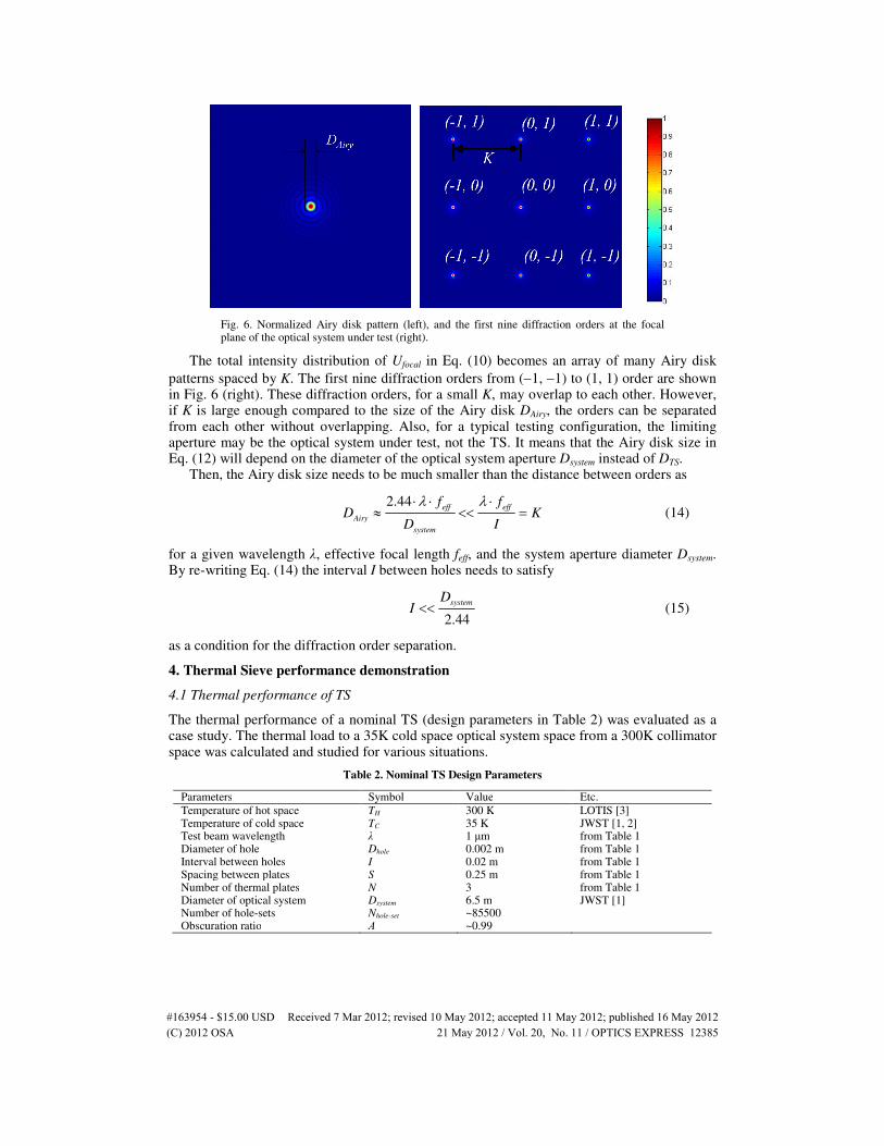
Fig. 6. Normalized Airy disk pattern (left), and the first nine diffraction orders at the focal plane of the optical system under test (right).

The total intensity distribution of Ufocal in Eq. (10) becomes an array of many Airy disk

patterns spaced by K. The first nine diffraction orders from (−1, −1) to (1, 1) order are shown in Fig. 6 (right). These diffraction orders, for a small K, may overlap to each other. However, if K is large enough compared to the size of the Airy disk DAiry, the orders can be separated from each other without overlapping. Also, for a typical testing configuration, the limiting aperture may be the optical system under test, not the TS. It means that the Airy disk size in Eq. (12) will depend on the diameter of the optical system aperture Dsystem instead of DTS.

Then, the Airy disk size needs to be much smaller than the distance between orders as

2.44

eff eff

Airy

system

f fD K

D I

λ λ⋅ ⋅ ⋅≈ << = (14)

for a given wavelength λ, effective focal length feff, and the system aperture diameter Dsystem. By re-writing Eq. (14) the interval I between holes needs to satisfy

2.44

systemDI << (15)

as a condition for the diffraction order separation.

4. Thermal Sieve performance demonstration

4.1 Thermal performance of TS

The thermal performance of a nominal TS (design parameters in Table 2) was evaluated as a case study. The thermal load to a 35K cold space optical system space from a 300K collimator space was calculated and studied for various situations.

Table 2. Nominal TS Design Parameters

Parameters Symbol Value Etc.

Temperature of hot space TH 300 K LOTIS [3] Temperature of cold space TC 35 K JWST [1, 2] Test beam wavelength λ 1 µm from Table 1 Diameter of hole Dhole 0.002 m from Table 1 Interval between holes I 0.02 m from Table 1 Spacing between plates S 0.25 m from Table 1 Number of thermal plates N 3 from Table 1 Diameter of optical system Dsystem 6.5 m JWST [1] Number of hole-sets Nhole-set ~85500 Obscuration ratio Α ~0.99


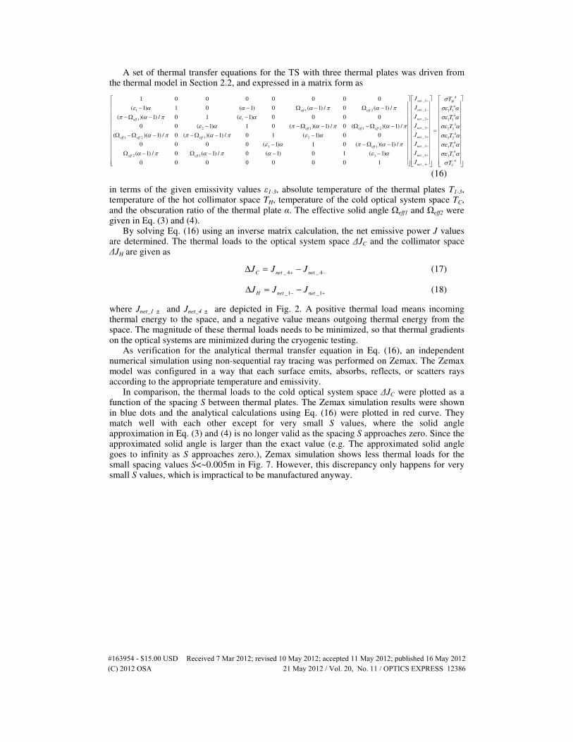
A set of thermal transfer equations for the TS with three thermal plates was driven from the thermal model in Section 2.2, and expressed in a matrix form as

1 1 2

1 1

2 1 1 2

1 2 1 2

3 1

1 0 0 0 0 0 0 0

( 1) 1 0 ( 1) 0 ( 1) / 0 ( 1) /

( )( 1) / 0 1 ( 1) 0 0 0 0

0 0 ( 1) 1 0 ( )( 1) / 0 ( )( 1) /

( )( 1) / 0 ( )( 1) / 0 1 ( 1) 0 0

0 0 0 0 ( 1) 1 0 ( )( 1)

eff eff

eff

eff eff eff

eff eff eff

eff

ε α α α π α ππ α π ε α

ε α π α π α πα π π α π ε α

ε α π α

− − Ω − Ω −

−Ω − −

− −Ω − Ω −Ω −

Ω −Ω − −Ω − −

− −Ω −

4_1

4_1 1 1

4_ 2 1 1

4_ 2 2 2

4_ 3 2 2

4_ 3 3 3

_ 42 1 3

_ 4

/

( 1) / 0 ( 1) / 0 ( 1) 0 1 ( 1)

0 0 0 0 0 0 0 1

net H

net

net

net

net

net

neteff eff

net

J T

J T

J T

J T

J T

J T

J

J

σσε ασε ασε ασε α

π σε αα π α π α ε α σε

+

−

+

−

+

−

+

−

= Ω − Ω − − −

4

3 3

4

C

T

T

ασ

(16)

in terms of the given emissivity values ε1-3, absolute temperature of the thermal plates T1-3, temperature of the hot collimator space TH, temperature of the cold optical system space TC, and the obscuration ratio of the thermal plate α. The effective solid angle Ωeff1 and Ωeff2 were given in Eq. (3) and (4).

By solving Eq. (16) using an inverse matrix calculation, the net emissive power J values are determined. The thermal loads to the optical system space ∆JC and the collimator space ∆JH are given as

_ 4 _ 4C net net

J J J+ −∆ = − (17)

_1 _1H net net

J J J− +∆ = − (18)

where Jnet_1 ± and Jnet_4 ± are depicted in Fig. 2. A positive thermal load means incoming thermal energy to the space, and a negative value means outgoing thermal energy from the space. The magnitude of these thermal loads needs to be minimized, so that thermal gradients on the optical systems are minimized during the cryogenic testing.

As verification for the analytical thermal transfer equation in Eq. (16), an independent numerical simulation using non-sequential ray tracing was performed on Zemax. The Zemax model was configured in a way that each surface emits, absorbs, reflects, or scatters rays according to the appropriate temperature and emissivity.

In comparison, the thermal loads to the cold optical system space ∆JC were plotted as a function of the spacing S between thermal plates. The Zemax simulation results were shown in blue dots and the analytical calculations using Eq. (16) were plotted in red curve. They match well with each other except for very small S values, where the solid angle approximation in Eq. (3) and (4) is no longer valid as the spacing S approaches zero. Since the approximated solid angle is larger than the exact value (e.g. The approximated solid angle goes to infinity as S approaches zero.), Zemax simulation shows less thermal loads for the small spacing values S<~0.005m in Fig. 7. However, this discrepancy only happens for very small S values, which is impractical to be manufactured anyway.


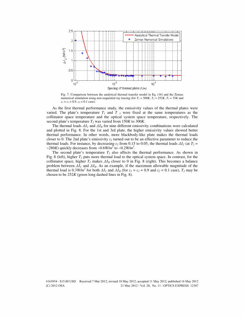
Fig. 7. Comparison between the analytical thermal transfer model in Eq. (16) and the Zemax numerical simulation using non-sequential ray tracing (for T1 = 300K, T2 = 252K, T3 = 35K and ε1 = ε3 = 0.9, ε2 = 0.1 case).

As the first thermal performance study, the emissivity values of the thermal plates were varied. The plate’s temperature T1 and T 3 were fixed at the same temperatures as the collimator space temperature and the optical system space temperature, respectively. The second plate’s temperature T2 was varied from 150K to 300K.

The thermal loads ∆JC and ∆JH for nine different emissivity combinations were calculated and plotted in Fig. 8. For the 1st and 3rd plate, the higher emissivity values showed better thermal performance. In other words, more blackbody-like plate makes the thermal loads closer to 0. The 2nd plate’s emissivity ε2 turned out to be an effective parameter to reduce the thermal loads. For instance, by decreasing ε2 from 0.15 to 0.05, the thermal loads ∆JC (at T2 = ~280K) quickly decreases from ~0.6W/m

2 to ~0.2W/m

2.

The second plate’s temperature T2 also affects the thermal performance. As shown in Fig. 8 (left), higher T2 puts more thermal load to the optical system space. In contrast, for the collimator space, higher T2 makes ∆JH closer to 0 in Fig. 8 (right). This becomes a balance problem between ∆JC and ∆JH. As an example, if the maximum allowable magnitude of the thermal load is 0.3W/m

2 for both ∆JC and ∆JH (for ε1 = ε3 = 0.9 and ε2 = 0.1 case), T2 may be

chosen to be 252K (green long dashed lines in Fig. 8).


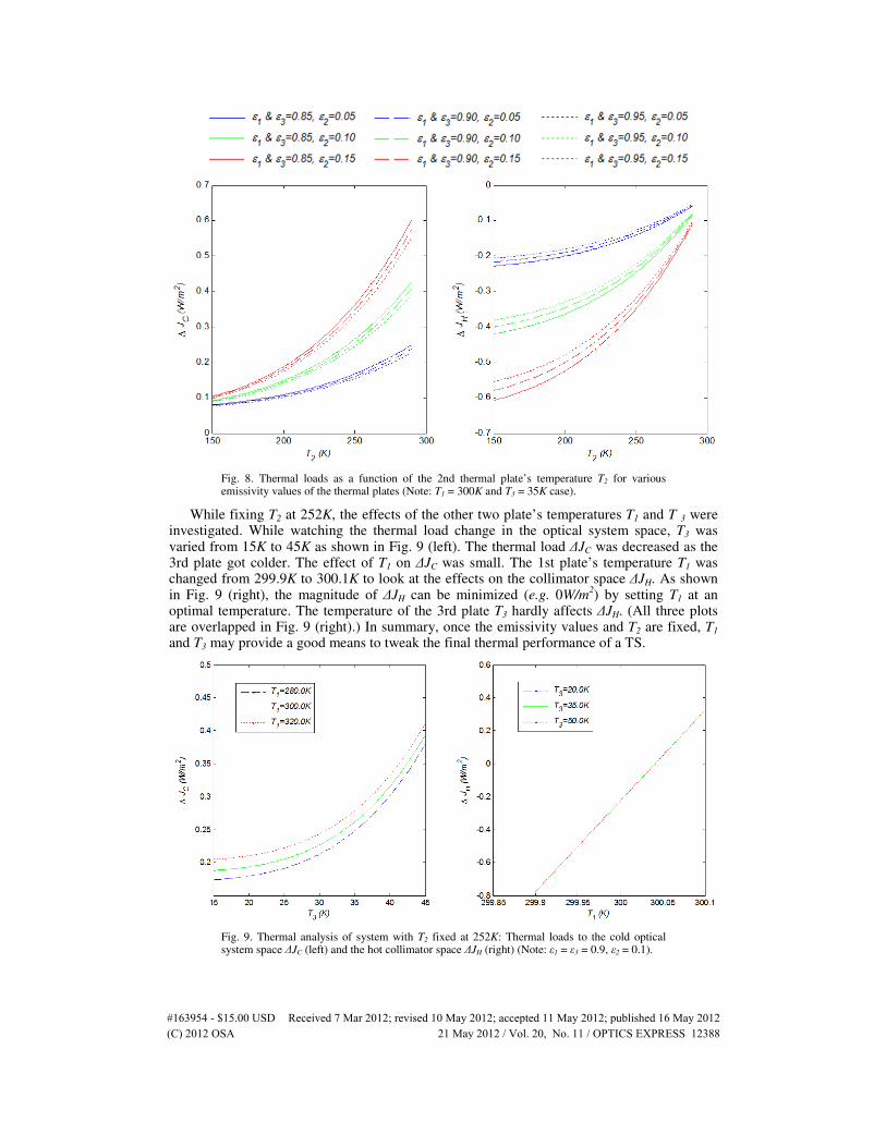
Fig. 8. Thermal loads as a function of the 2nd thermal plate’s temperature T2 for various emissivity values of the thermal plates (Note: T1 = 300K and T3 = 35K case).

While fixing T2 at 252K, the effects of the other two plate’s temperatures T1 and T 3 were investigated. While watching the thermal load change in the optical system space, T3 was varied from 15K to 45K as shown in Fig. 9 (left). The thermal load ∆JC was decreased as the 3rd plate got colder. The effect of T1 on ∆JC was small. The 1st plate’s temperature T1 was changed from 299.9K to 300.1K to look at the effects on the collimator space ∆JH. As shown in Fig. 9 (right), the magnitude of ∆JH can be minimized (e.g. 0W/m

2) by setting T1 at an

optimal temperature. The temperature of the 3rd plate T3 hardly affects ∆JH. (All three plots are overlapped in Fig. 9 (right).) In summary, once the emissivity values and T2 are fixed, T1 and T3 may provide a good means to tweak the final thermal performance of a TS.

Fig. 9. Thermal analysis of system with T2 fixed at 252K: Thermal loads to the cold optical system space ∆JC (left) and the hot collimator space ∆JH (right) (Note: ε1 = ε3 = 0.9, ε2 = 0.1).


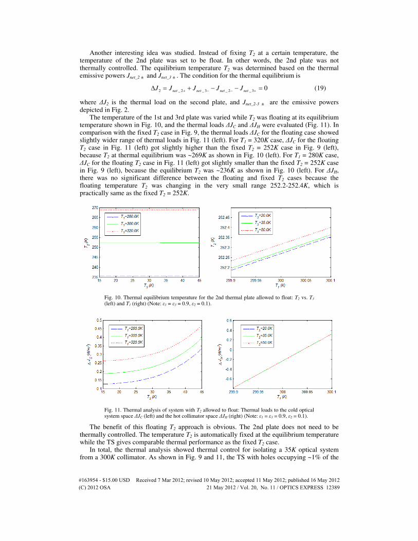
Another interesting idea was studied. Instead of fixing T2 at a certain temperature, the temperature of the 2nd plate was set to be float. In other words, the 2nd plate was not thermally controlled. The equilibrium temperature T2 was determined based on the thermal emissive powers Jnet_2 ± and Jnet_3 ± . The condition for the thermal equilibrium is

2 _ 2 _ 3 _ 2 _ 3

0net net net net

J J J J J+ − − +∆ = + − − = (19)

where ∆J2 is the thermal load on the second plate, and Jnet_2-3 ± are the emissive powers depicted in Fig. 2.

The temperature of the 1st and 3rd plate was varied while T2 was floating at its equilibrium temperature shown in Fig. 10, and the thermal loads ∆JC and ∆JH were evaluated (Fig. 11). In comparison with the fixed T2 case in Fig. 9, the thermal loads ∆JC for the floating case showed slightly wider range of thermal loads in Fig. 11 (left). For T1 = 320K case, ∆JC for the floating T2 case in Fig. 11 (left) got slightly higher than the fixed T2 = 252K case in Fig. 9 (left), because T2 at thermal equilibrium was ~269K as shown in Fig. 10 (left). For T1 = 280K case, ∆JC for the floating T2 case in Fig. 11 (left) got slightly smaller than the fixed T2 = 252K case in Fig. 9 (left), because the equilibrium T2 was ~236K as shown in Fig. 10 (left). For ∆JH, there was no significant difference between the floating and fixed T2 cases because the floating temperature T2 was changing in the very small range 252.2-252.4K, which is practically same as the fixed T2 = 252K.

Fig. 10. Thermal equilibrium temperature for the 2nd thermal plate allowed to float: T2 vs. T3 (left) and T1 (right) (Note: ε1 = ε3 = 0.9, ε2 = 0.1).

Fig. 11. Thermal analysis of system with T2 allowed to float: Thermal loads to the cold optical system space ∆JC (left) and the hot collimator space ∆JH (right) (Note: ε1 = ε3 = 0.9, ε2 = 0.1).

The benefit of this floating T2 approach is obvious. The 2nd plate does not need to be thermally controlled. The temperature T2 is automatically fixed at the equilibrium temperature while the TS gives comparable thermal performance as the fixed T2 case.

In total, the thermal analysis showed thermal control for isolating a 35K optical system from a 300K collimator. As shown in Fig. 9 and 11, the TS with holes occupying ~1% of the


thermal plate area and with two black (i.e. high emissivity) and a polished (i.e. low emissivity) thermal plates accomplished thermal loads less than 200mW/m

2 for both the ambient and the

cryogenic sides of the testing configuration. This is nearly 4 orders of magnitude attenuation from the 300K collimator’s radiating power.

4.2 Optical performance of TS

The test beam in an optical testing configuration with TS goes through the array of holes. A perfectly engineered TS may be fully modeled, simulated and calibrated. However, any actual TS will have variations in mechanical dimensions, which can include each hole’s diameter, locations due to misalignment, manufacturing tolerance and thermal deformation. This does not seriously harm the thermal performance of the TS, but does affect the optical performance.

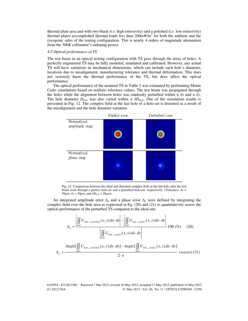
The optical performance of the nominal TS in Table 2 was estimated by performing Monte Carlo simulations based on realistic tolerance values. The test beam was propagated through the holes while the alignment between holes was randomly perturbed within ± δx and ± δy. The hole diameter Dhole was also varied within ± δDhole. One of the simulation results is presented in Fig. 12. The complex field at the last hole of a hole-set is distorted as a result of the misalignment and the hole diameter variation.

Fig. 12. Comparison between the ideal and distorted complex field at the last hole after the test beam went through a perfect hole-set and a perturbed hole-set, respectively. (Tolerance: δx = 50µm, δy = 50µm, and δDhole = 20µm).

An integrated amplitude error ∆a and a phase error ∆p were defined by integrating the complex field over the hole area as expressed in Eq. (20) and (21) to quantitatively assess the optical performance of the perturbed TS compared to the ideal one.

_ _

_

( , ) ( , )

100 (%)

( , )

hole perturbed hole perfect

hole hole

a

hole perfect

hole

U x y dx dy U x y dx dy

U x y dx dy

⋅ − ⋅

∆ = ⋅

⋅

∫∫ ∫∫

∫∫ (20)

_ _[ ( , ) ] [ ( , ) ]

( )2

hole perturbed hole perfect

hole hole

p

Angle U x y dx dy Angle U x y dx dy

wavesπ

⋅ − ⋅

∆ =⋅

∫∫ ∫∫(21)


where Angle is a function returns the phase angle of a complex field. These definitions simplify the representation and evaluation process of the test beam quality in ~85500 hole-sets.

Variations in amplitude cause intensity fluctuations across the pupil

100 2 100 2i a

Q A

Q A

∆ ∆∆ = ⋅ ≅ ⋅ ⋅ = ⋅∆ (22)

when small ∆A value is present since the intensity Q is the square of amplitude A. Variations in phase cause wavefront phase to change across the pupil, which degrade the performance of the collimator. The form of the wavefront phase or intensity variation follows the changes in hole size and position. For example, if all the holes are shifted by a same amount, the intensity will be decreased uniformly across the pupil. If holes in a small region are shifted relative to rest of the system, the intensity of the light in that region will be decreases and the wavefront phase in that region will be shifted.

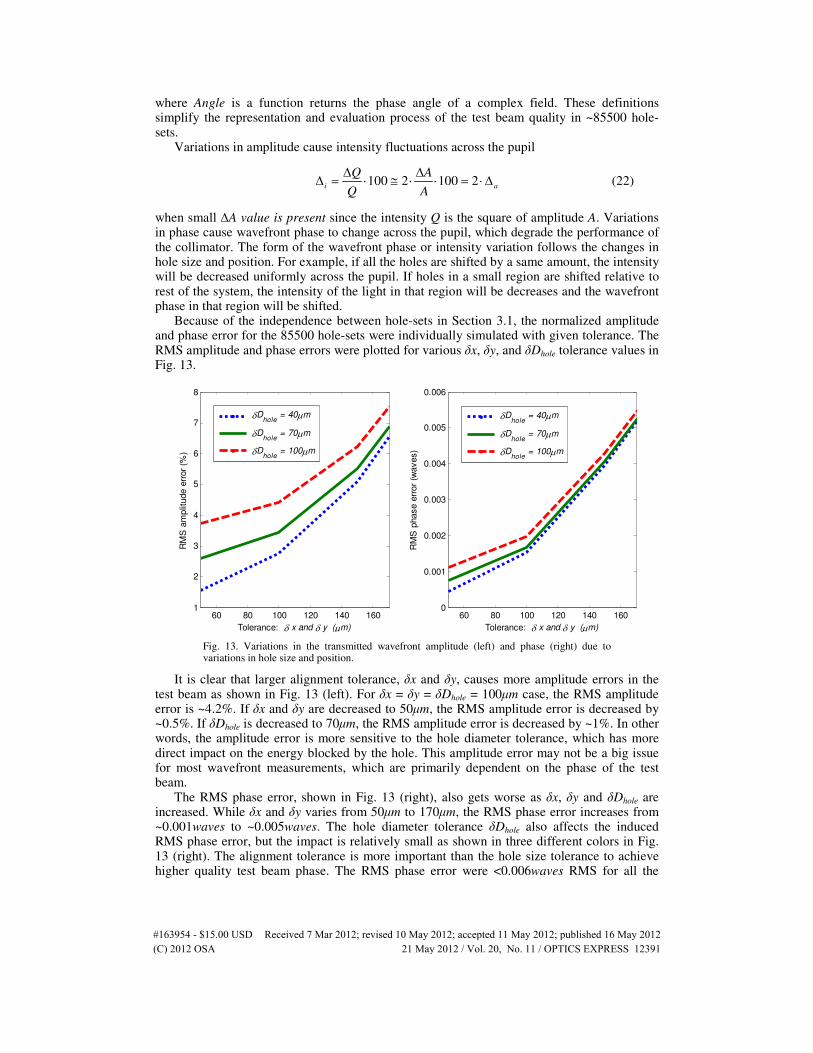
Because of the independence between hole-sets in Section 3.1, the normalized amplitude and phase error for the 85500 hole-sets were individually simulated with given tolerance. The RMS amplitude and phase errors were plotted for various δx, δy, and δDhole tolerance values in Fig. 13.

60 80 100 120 140 1601

2

3

4

5

6

7

8

Tolerance: δ x and δ y (µm)

RM

S a

mplit

ude e

rror

(%)

δDhole

= 40µm

δDhole

= 70µm

δDhole

= 100µm

60 80 100 120 140 1600

0.001

0.002

0.003

0.004

0.005

0.006

Tolerance: δ x and δ y (µm)

RM

S p

hase e

rror

(waves)

δDhole

= 40µm

δDhole

= 70µm

δDhole

= 100µm

Fig. 13. Variations in the transmitted wavefront amplitude (left) and phase (right) due to variations in hole size and position.

It is clear that larger alignment tolerance, δx and δy, causes more amplitude errors in the test beam as shown in Fig. 13 (left). For δx = δy = δDhole = 100µm case, the RMS amplitude error is ~4.2%. If δx and δy are decreased to 50µm, the RMS amplitude error is decreased by ~0.5%. If δDhole is decreased to 70µm, the RMS amplitude error is decreased by ~1%. In other words, the amplitude error is more sensitive to the hole diameter tolerance, which has more direct impact on the energy blocked by the hole. This amplitude error may not be a big issue for most wavefront measurements, which are primarily dependent on the phase of the test beam.

The RMS phase error, shown in Fig. 13 (right), also gets worse as δx, δy and δDhole are increased. While δx and δy varies from 50µm to 170µm, the RMS phase error increases from ~0.001waves to ~0.005waves. The hole diameter tolerance δDhole also affects the induced RMS phase error, but the impact is relatively small as shown in three different colors in Fig. 13 (right). The alignment tolerance is more important than the hole size tolerance to achieve higher quality test beam phase. The RMS phase error were <0.006waves RMS for all the


tolerance ranges investigated in this section, which seems promising for most optical testing applications.

5. Concluding remarks

A new conceptual testing configuration to test a cryogenic optical system inside a vacuum chamber was introduced with the Thermal Sieve. The TS provides thermal decoupling between a cryogenic optical system under test and a collimator operating at ambient temperature, while passing the test beam wavefront without significant degradation.

The feasibility of the conceptual configuration was demonstrated in two areas. The thermal performance was analyzed based on the analytical thermal transfer model. The final results looked promising for isolating a 30K system from a 300K collimator. A three thermal plate TS will cause thermal loading less than 200mW/m

2 for both the ambient and the

cryogenic sides of the system. The optical performance was demonstrated with the wave propagation simulation results showing that the wavefront degradation due to the TS was very small (e.g. <0.006waves RMS).

This conceptual study based on the theoretical analysis and numerical simulations provides a good baseline for the further developments of this new testing configuration. However, we acknowledge that the simplified models and approximated equations in this study such as thermal transfer equations, integrated amplitude and phase error may not fully describe the real performance of TS. Also, there might be some second order effects. For instance, the primary mirror of a collimator may focus some of the thermal radiation to its secondary mirror. The actual thermal and optical performance, which will be a function of many complex factors, must be experimentally demonstrated using a proof-of-concept configuration. We are currently proposing an experimental demonstration using a sub-scale TS inside a cryogenic vacuum chamber.

Appendix

A.1 Basic functions

Because Fourier transform is frequently used in the course of analytical wave propagation in Section 3, it is convenient to define some basic functions.

Cylinder function, cyl(r), which gives a circular disk in the x-y plane, is defined as below.

2 2

2 2

2 2

1 , 1/ 2( )

0 , 1/ 2

x ycyl x y

x y

+ ≤+ =

+ > (23)

Sombrero function, somb(r), is defined using the first-order Bessel function of the first kind, J1.

2 2

2 2 1

2 2

2 ( )( )

J x ysomb x y

x y

π

π

⋅ ++ =

⋅ + (24)

The 2D comb function, comb(x, y), is defined as

( , ) ( , )m n

comb x y x m y nδ∞ ∞

=−∞ =−∞

= − −∑ ∑ (25)

where δ(x, y) is the delta function.


Documents

Use of thermal sieve to allow optical testing of cryogenic ... · PDF fileThe main function of a Thermal Sieve is ... passes through the 1st plate holes. The collimator and optical