Use of the IHACRES rainfall-runoff model in arid and semi

arid regions

B.F.W. Croke and A.J. Jakeman Integrated Catchment Assessment and Management Centre, School for Resources,

Environment and Society, and Centre for Resource and Environmental Studies, The

Australian National University, Canberra, Australia

ABSTRACT: Streamflow in arid and semi-arid regions tends to be dominated by rapid responses to

intense rainfall events. Such events frequently have a high degree of spatial variability, coupled with

poorly gauged rainfall data. This sets a fundamental limit on the capacity of any rainfall-runoff model

to reproduce the observed flow. The IHACRES model is a parameterically efficient rainfall-runoff

model that has been applied to a large number of catchments covering a diverse range of

climatologies. While originally designed for more temperate climates, the model has been

successfully applied to a number of ephemeral streams in Australia. The recent release of

IHACRES_v2.0 includes this modified loss module, as well as a cross correlation analysis tool, new fit

indicators and visualisation tools. Additional advances that will be included in future releases of the

IHACRES model include: an alternative non-linear loss module which has a stronger physical basis, at

the cost of a slightly more complicated calibration procedure; a baseflow filtering approach that uses

the SRIV algorithm to estimate the parameter values; a modified routing module that includes the

influence of groundwater losses (subsurface outflow and extraction of groundwater); and a technique

to estimate the response curve directly from observed streamflow data.

INTRODUCTION

Successful management of water resources requires qualitative analysis of the effects of changes in

climate and land use practices on streamflow and water quality. While expert knowledge can provide

indications of such impacts, detailed analysis requires the use of mathematical models to separate the

water balance dynamically (at the temporal scale at which the important processes are operating).

This includes separation of incident precipitation into losses to evapotranspiration, runoff to streams,

recharge to groundwater systems and changes in short-term catchment storages. Some of the

processes which need to be considered are: evapotranspiration and feedback to the atmosphere;

vegetation dynamics; groundwater levels and the resulting effect on soil waterlogging and salinisation;

reservoir storage capacity reliability; wetland dynamics; urban runoff; flooding; erosion in crop and

pasture lands, as well as channel erosion and sedimentation; and aquatic ecosystem functions.

Arid and semi-arid areas tend to be dominated by intense rainfall events with a high degree of spatial

variability. This typically leads to a rapid response profile, and in areas without weather radar

coverage, poor rain gauge density prevents accurate estimation of the rainfall depth and spatial

distribution for a particular event. Further, if only daily rainfall data are available, then calibrating a

rainfall-runoff model at a daily timestep means that most of the information contained in the

hydrograph is not used (note that runoff here means total streamflow, not just surface runoff).

Another important consideration for calibration of models for catchments in arid and semi-arid areas is

the frequency of events. Such catchments tend to have fewer streamflow events than catchments in

wetter climates. This means that longer calibration periods are needed in order to reduce the

uncertainty in model parameters. Otherwise, parameter values will tend to relate more to the errors in

the data, with a significant decrease in performance in simulation compared with calibration.

IHACRES RAINFALL-RUNOFF MODEL

Data availability

Typically the available data for catchments (other than heavily instrumented research catchments) is

limited to daily rainfall and temperature and, in some cases, stream discharge. Thus the mathematical

representation most often used is a rainfall-runoff model. Rainfall-runoff models fall into several

categories: metric, conceptual and physics-based models (Wheater et al., 1993). Metric models are

typically the most simple, using observed data (rainfall and streamflow) to characterise the response of

a catchment. Conceptual models impose a more complex representation of the internal processes

involved in determining catchment response, and can have a range of complexity depending on the

structure of the model. Physics-based models involve numerical solution of the relevant equations of

motion.

Model structure

The selection of which model to use should be based on the issue(s) being investigated and the data

available. As more complex questions are asked, more complex models are needed to provide the

answers. However, with increasing model complexity comes the cost of increasing uncertainty in the

model predictions. The IHACRES model is a hybrid conceptual-metric model, using the simplicity of

the metric model to reduce the parameter uncertainty inherent in hydrological models while at the

same time attempting to represent more detail of the internal processes than is typical for a metric

model. Figure 1 shows the generic structure of the IHACRES model. It contains a non-linear loss

module which converts rainfall into effective rainfall (that portion which eventually reaches the stream

prediction point) and a linear module which transfers effective rainfall to stream discharge. Further

modules can be added including one that allows recharge to be output. The inclusion of a range of

non-linear loss modules within IHACRES increases its flexibility in being used to access the effects of

climate and land use change. The linear module routes effective rainfall to stream through any

configuration of stores in parallel and/or in series. The configuration of stores is identified from the time

series of rainfall and discharge but is typically either one store only, representing ephemeral streams,

or two in parallel, allowing baseflow or slowflow to be represented as well as quickflow. Only rarely

does a more complex configuration than this improve the fit to discharge measurements (Jakeman

and Hornberger, 1993).

Figure 1: Generic structure of the IHACRES model, showing the conversion of climate time series data to

effective rainfall using the Non-linear Module, and the Linear Module converting effective rainfall to

streamflow time series.

The original structure of the IHACRES model used an exponentially decaying soil moisture index to

convert rainfall into effective rainfall. Ye et al. (1997) adapted this model to improve the performance

of the model in ephemeral catchments. This involved introducing a threshold parameter (l) and a non-

linear relationship (power law with exponent parameter p) between the soil moisture index and the

fraction of rainfall that becomes effective rainfall.

The Ye et al. (1997) version has been coded within IHACRES_v2.0, reformulated to enable the mass

balance parameter c (see below) to be estimated from the gain of the transfer function, and to reduce

the interaction between the c and p parameters. The effective rainfall uk in the revised model is given

by:

( )[ ] kp

kk rlcu −= φ (1)

where rk is the observed rainfall, c, l and p are parameters (mass balance, soil moisture index

threshold and non-linear response terms, respectively), and φk is a soil moisture index given by:

( ) 111 −−+= kkkk r φτφ (2)

with the drying rate τk given by:

( )( )krwk TTf −= 062.0expττ (3)

where τw, f and Tr are parameters (reference drying rate, temperature modulation and reference

temperature, respectively). This formulation enables the gain of the transfer function to be directly

related to the value of the parameter c, thus simplifying model calibration. This version of the model is

more general than the version used within the IHACRES_PC model (Littlewood et al. 1997) which can

be recovered by setting parameters l to zero and p to one (with the soil moisture index in the original

model given by sk = cφk). This version of the non-linear module is described in detail in Jakeman et al.

(1990) and Jakeman and Hornberger (1993). Examples of studies that have used this version of

IHACRES (with minor modifications to the Equation 3) can be found in Hansen et al. (1996), Post and

Jakeman (1999), Schreider et al. (1996) and Ye et al. (1997).

Regionalisation

Various versions of the IHACRES model have also been used to address regionalisation issues (Post

and Jakeman, 1996; Sefton and Howarth, 1998; Kokkonen et al, 2003). These issues require methods

for estimating the parameters of models from independent means such as landscape attributes rather

than directly from rainfall-discharge time series. The parametric efficiency of IHACRES (often about six

parameters) lends itself to regionalisation problems, making it easier than complex models to relate its

parameters to landscape attributes. The IHACRES model is one of the models to be used by the Top-

Down modelling Working Group (Littlewood et al. 2003) operating as part of the Prediction in

Ungauged Basins initiative of the International Association of Hydrological Sciences

(http://cee.uiuc.edu/research/pub/).

NEW VERSION OF IHACRES

There are a number of reasons for the development of a Java-based version of the rainfall-runoff

model IHACRES. This includes several recent developments in the model, particularly with respect to

the non-linear loss module. One such modification is the development of a catchment moisture deficit

(CMD) accounting system that enables a more process-based determination of the partitioning of

rainfall to discharge and evapotranspiration (Croke and Jakeman, 2004). Other enhancements

include simulating the effects of retention storages such as farm dams on stream discharge (Schreider

et al., 1999) as well as the interaction between groundwater recharge and streamflow by linking a

physics-based groundwater discharge model (Sloan, 2000) with the IHACRES model (Croke et al.

2002). The groundwater version of the model was used to assess groundwater recharge in the

Jerrabomberra Creek catchment, ACT (Croke et al., 2001). These developments have improved the

potential of IHACRES to model the effects of land use change on catchment response (eg Dye and

Croke, 2003), as well as inferring the hydrological response of ungauged catchments.

Further advances in the IHACRES model have been made in the method of calibration. In addition to

the current simple refined instrumental variable (SRIV) method of parameter estimation (eg Jakeman

et al., 1990), a method based on estimating hydrographs directly from streamflow data without the

need for rainfall data has been developed (Croke, 2004). This enables higher resolution streamflow

data to be used, reducing the loss of information that occurs when data is binned to a daily timestep.

In addition, this calibration method reduces the number of parameters that need to be estimated within

the model, thus reducing the parameter uncertainty, while at the same time reducing the time required

to calibrate the model.

In order to visualise data such as inputs and model outputs, the new Java-based version of IHACRES

makes use of the VisAD library. VisAD (Hibbard, 1998) is a Java component library for interactive

visualisation and analysis of numerical data. The library is available under the Lesser General Public

License (LGPL), which allows the library to be used in commercial applications so long as certain

conditions are satisfied. Using VisAD it has been possible to create very sophisticated interactive

visualisations of data within IHACRES_v2.0 with a minimum amount of effort. The visualisation of data

is very important for the calibration and interpretation of models like IHACRES_v2.0 where it is

necessary for users to be able to view effective representations of data in order to make appropriate

decisions.

A number of changes have been made to the objective functions used in IHACRES_v2.0. The lag 1

correlation coefficients U1 (correlation coefficient of the lagged effective rainfall and model error) and

X1 (correlation coefficient of the lagged modelled streamflow and the model error) have been

normalised correctly (e.g. a value of +1 corresponds to perfect correlation) to aid in interpretation of

these values. Also, a number of objective functions have been added. These are based on the Nash-

Sutcliffe model efficiency indicator:

( )

( )∑

∑

−

−−=

ioio

iimio

QQ

QQR

2,

2,,

2 1 (4)

with the observed flow Qo, and modelled flow Qm replaced with the square root (R2_sqrt), logarithm

(R2_log) and inverse (R2_inv) of the flow. These objective functions are progressively less biased to

peak flows, and more to low flows. In arid and semi-arid catchments, the best objective function is

likely to be R2_sqrt as there is rarely a baseflow component in these catchments.

To avoid numerical errors with the logarithmic and inverse versions, the 90% flow exceedence value

(ignoring time steps with no flow) was added to Qo. These shift the weighting of the objective function

progressively from the flow peaks to low flows. The logarithmic form, for example, gives a fairly

uniform weighting to high and low flows, while the inverse version is heavily biased towards low flows.

Subsequently, for studies focused on flood peaks, the traditional Nash-Sutciffe efficiency should be

used. However, where simulating low flows are important (e.g. ecological impacts, estimating

availability of water for irrigation), the logarithmic or inverse forms of the efficiency indicator should be

used.

APPLICATION OF THE MODEL TO AUSTRALIAN CATCHMENTS

A significant fraction of Australia is class as arid or semi-arid (see Figure 2). Catchments from three

different climatic regions are presented here: The Canning River in Western Australia, the Liverpool

Plains region of the Namoi River catchment in northern NSW, and the Burdekin River catchment in

northern Queensland.

Figure 2: Ratio of rainfall to potential evaporation across Australia (Rainfall and Potential Evaporation

data from the National Land and Water Resources Audit database (http://adl.brs.gov.au/ADLsearch/).

Canning River

The Canning River is a tributary of the Swan River, and is located southeast of Perth in Western

Australia. Data for the gauge at Scenic Drive (616024) has been used to test the IHACRES model.

This gauge is upstream of Canning Dam, and has a contributing area of 517km2. The data consist of

rainfall, streamflow and potential evaporation covering the period from 1/1/1977 to 31/12/1987, with all

data expressed in mm. The catchment has a Mediterranean climate, with about 80% of the rainfall

occurring between May and October. The river is ephemeral, with no flow approximately 54% of the

time. For the 11 years from 1978 to 1987, the mean annual rainfall was 890 mm, the runoff coefficient

was 1.8% and ratio of rainfall to potential evaporation was 0.64 (using the NLWRA data, the ratio of

rainfall to potential evaporation was 0.57). Thus, while the catchment is ephemeral, it is just above the

threshold for being classed as semi-arid (semi-arid catchments are defined as having P/PE values

between 0.2 and 0.5).

Figure 3 Swan River catchment area. The boundary of the catchment for gauge 616024 is shown in black.

The catchment was calibrated on a five year period from January 1, 1978 to December 31, 1982)

using the modified Ye et al. non-linear loss module (equations 1 to 3). Since a time series of potential

evaporation was used for the variation in the drying rate (rather than the more usual temperature), the

reference temperature was set to zero. Calibration runs showed that the model was unable to

reproduce the observed flows if the threshold parameter (l) was fixed at 0, and the non-linearity

parameter (p) fixed at 1. Introducing the threshold parameter resulted in a considerable improvement

in the model fit, with R2 values reaching 0.93 for the calibration period. The calibrated parameter

values were selected based on the R2_log objective function, and are shown in

Table 1.

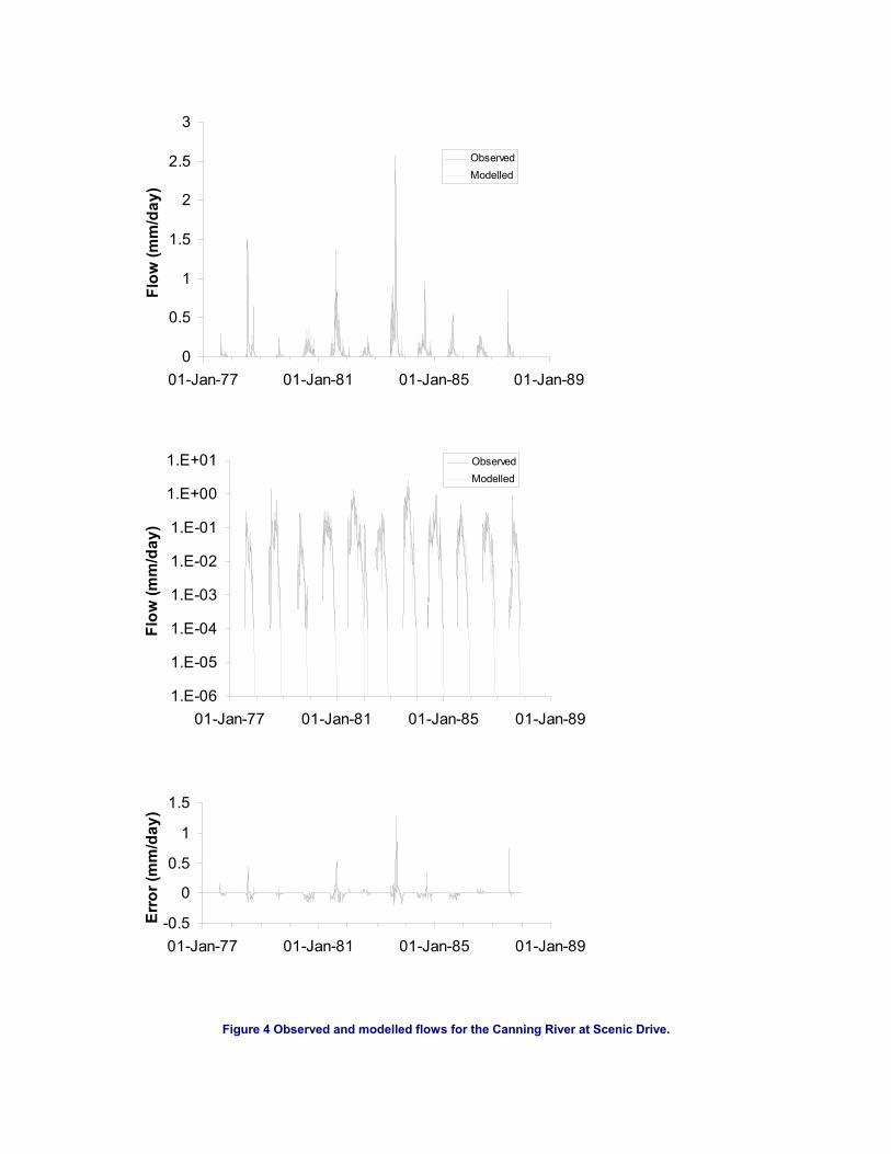
The calibrated model gave objective function values: R2 = 0.90, R2_sqrt = 0.93, R2_log = 0.95 and

R2_inv = 0.93 for the calibration period. For the remainder of the data, the values for the objective

functions were R2 = 0.87, R2_sqrt = 0.95, R2_log = 0.97 and R2_inv = 0.96. This shows that, except

for the R2 objective function, the model performed slightly better in the simulation period than in the

calibration period. Analysis of the statistics for individual years shows that the model performed very

poorly in 1980 (R2 = 0.22) and poorly in 1987 (R2 = 0.55). All other years gave R2 values of greater

than or equal to 0.84 with the exception of 1977 (R2 = 0.79) and 1979 (R2 = 0.72).

0

0.5

1

1.5

2

2.5

3

01-Jan-77 01-Jan-81 01-Jan-85 01-Jan-89

Flow

(mm

/day

)ObservedModelled

1.E-06

1.E-05

1.E-04

1.E-03

1.E-02

1.E-01

1.E+00

1.E+01

01-Jan-77 01-Jan-81 01-Jan-85 01-Jan-89

Flow

(mm

/day

)

ObservedModelled

-0.5

0

0.5

1

1.5

01-Jan-77 01-Jan-81 01-Jan-85 01-Jan-89

Erro

r (m

m/d

ay)

Figure 4 Observed and modelled flows for the Canning River at Scenic Drive.

Namoi River catchments

The Liverpool Plains region of the Namoi River catchment is located in northern NSW, Australia. This

area is semi-arid, with a ratio of P/PE of between 0.4 and 0.5 for most of the area (except for the

Liverpool Range to the south). The main rivers in the region are the Mooki River and Coxs Creek,

which drain north from the Liverpool Ranges to the Namoi River.

Figure 5 Liverpool Plains area of the Namoi River catchment. The boundary of gauge 419034 is shown in

grey, and that for gauge 419052 in black.

419034 This gauge is located on the Mooki River at Caroona, and corresponds to a catchment area of 2540

km2. The catchment was calibrated on a five year period from January 1, 1981 to December 31,

1985) again using the modified Ye et al. non-linear loss module. The calibrated parameter values

were selected based on the R2_sqrt objective function, and are shown in

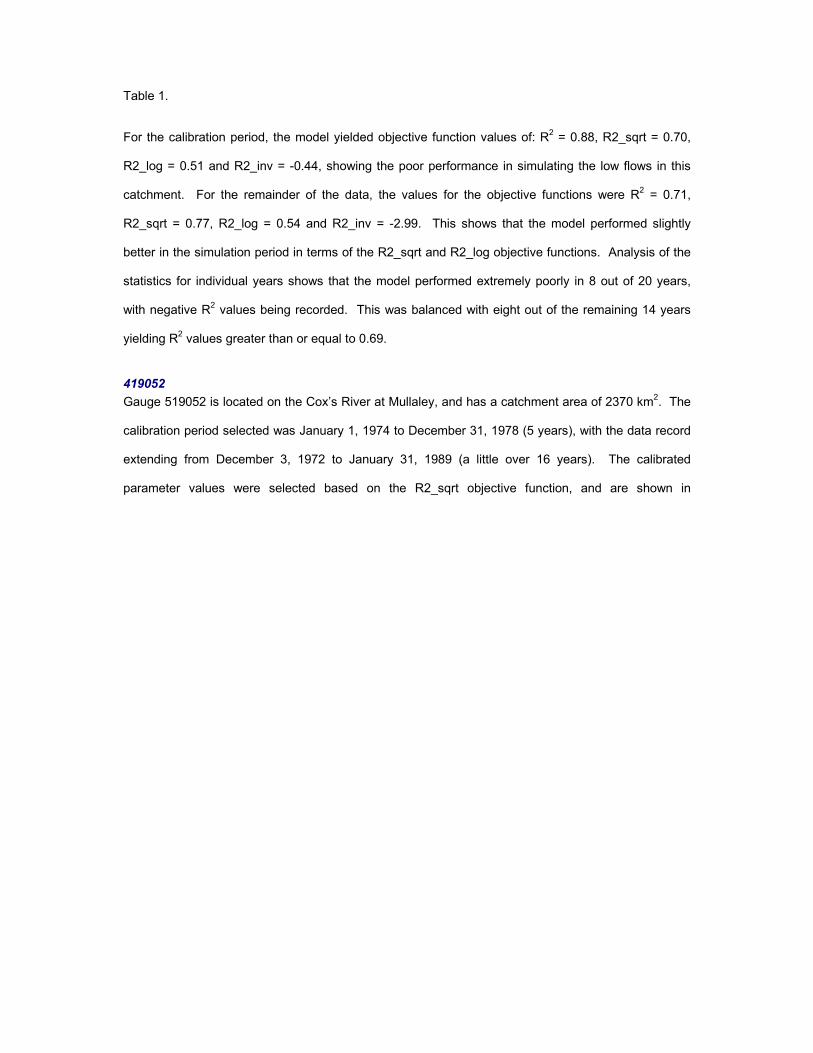
Table 1.

For the calibration period, the model yielded objective function values of: R2 = 0.88, R2_sqrt = 0.70,

R2_log = 0.51 and R2_inv = -0.44, showing the poor performance in simulating the low flows in this

catchment. For the remainder of the data, the values for the objective functions were R2 = 0.71,

R2_sqrt = 0.77, R2_log = 0.54 and R2_inv = -2.99. This shows that the model performed slightly

better in the simulation period in terms of the R2_sqrt and R2_log objective functions. Analysis of the

statistics for individual years shows that the model performed extremely poorly in 8 out of 20 years,

with negative R2 values being recorded. This was balanced with eight out of the remaining 14 years

yielding R2 values greater than or equal to 0.69.

419052 Gauge 519052 is located on the Cox’s River at Mullaley, and has a catchment area of 2370 km2. The

calibration period selected was January 1, 1974 to December 31, 1978 (5 years), with the data record

extending from December 3, 1972 to January 31, 1989 (a little over 16 years). The calibrated

parameter values were selected based on the R2_sqrt objective function, and are shown in

Table 1.

For the calibration period, the model yielded objective function values of: R2 = 0.86, R2_sqrt = 0.86,

R2_log = 0.77 and R2_inv = 0.39, showing better performance in simulating the low flows in this

catchment compared with gauge 419034. For the remainder of the data, the values for the objective

functions were R2 = 0.59, R2_sqrt = 0.65, R2_log = 0.82 and R2_inv = 0.71. This shows that the

model performed slightly better in simulating the low flows for the simulation period (R2_log and

R2_inv objective functions). Analysis of the statistics for individual years shows that the model

performed extremely poorly in 7 out of 16 years (some of the driest years in the data), with negative R2

values being recorded. There were 4 years with R2 values greater than 0.66, three of these in the

calibration period.

The poor R2_inv value for both catchments is a result of not including a slow flow component in the

model. This is evident in the log plots in Figure 6 and Figure 7. While these catchments have a slow

flow component, it is not easily identifiable using the en-bloc method. For gauge 419052, the

intermittent nature of the slow flow component is another problem that needs to be addressed.

0

50

100150

200

250

300350

400

450

01-Jan-77 01-Jan-81 01-Jan-85 01-Jan-89 01-Jan-93

Flow

(mm

/day

)

ObservedModelled

1.E-06

1.E-05

1.E-04

1.E-03

1.E-021.E-01

1.E+00

1.E+01

1.E+02

1.E+03

01-Jan-77 01-Jan-81 01-Jan-85 01-Jan-89 01-Jan-93

Flow

(mm

/day

)

ObservedModelled

-100

0

100

200

300

01-Jan-77 01-Jan-81 01-Jan-85 01-Jan-89 01-Jan-93

Erro

r (m

m/d

ay)

Figure 6. Observed and modelled flow for gauge 419034

0

100

200

300

400

500

600

700

800

01-Jan-73 01-Jan-77 01-Jan-81 01-Jan-85

Flow

(mm

/day

)

ObservedModelled

1.E-06

1.E-05

1.E-04

1.E-03

1.E-021.E-01

1.E+00

1.E+01

1.E+02

1.E+03

01-Jan-73 01-Jan-77 01-Jan-81 01-Jan-85

Flow

(mm

/day

)

ObservedModelled

-300-200-100

0100200300

01-Jan-73 01-Jan-77 01-Jan-81 01-Jan-85

Erro

r (m

m/d

ay)

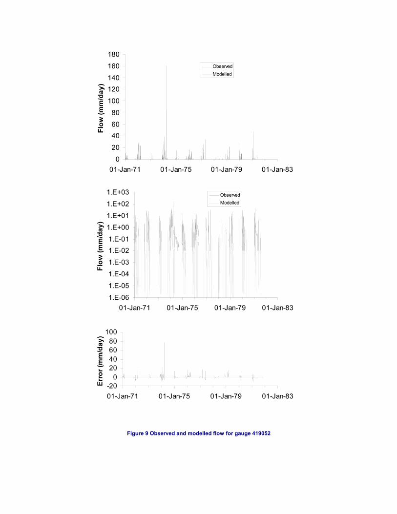
Figure 7 Observed and modelled flow for gauge 419052.

Burdekin River

The Burdekin River is a large (area approximately 130000 km2) coastal catchment in northern

Queenland. The catchment has a dry tropical climate, with rainfall dominated by high intensity events.

The data used in this tutorial is for gauge 120014 (Broughton River at Oak Meadows, area 181 km2).

The data extends from November 8, 1970 to December 31, 1987. The data consist of rainfall (mm),

streamflow (cumecs) and temperature (oC). The mean annual rainfall from 1/1/1980 to 31/12/1999

was 590 mm, and ratio of rainfall to potential evaporation was 0.32 (derived from rainfall and potential

evaporation surfaces obtained from the National Land and Water Resources Audit database

http://adl.brs.gov.au/ADLsearch/).

For the calibration period, the model yielded objective function values of: R2 = 0.76, R2_sqrt = 0.82,

R2_log = 0.92 and R2_inv = 0.91, showing better performance in simulating the low flows in this

catchment compared with the gauges in the Namoi River catchment. For the remainder of the data,

the values for the objective functions were R2 = 0.72, R2_sqrt = 0.78, R2_log = 0.87 and R2_inv =

0.89. This is the result of the lack of any baseflow component in this catchment. Analysis of the

statistics for individual years shows that the model performed extremely poorly in 2 out of 17 years

(some of the driest years in the data), with negative R2 values being recorded. There were 7 years

with R2 values greater than 0.6, three of these in the calibration period.

Figure 8 Northern part of the Burdekin River catchment, with catchment for gauge 120014

outlined in black.

0

20

4060

80

100

120140

160

180

01-Jan-71 01-Jan-75 01-Jan-79 01-Jan-83

Flow

(mm

/day

)

ObservedModelled

1.E-06

1.E-05

1.E-04

1.E-03

1.E-021.E-01

1.E+00

1.E+01

1.E+02

1.E+03

01-Jan-71 01-Jan-75 01-Jan-79 01-Jan-83

Flow

(mm

/day

)

ObservedModelled

-200

20406080

100

01-Jan-71 01-Jan-75 01-Jan-79 01-Jan-83

Erro

r (m

m/d

ay)

Figure 9 Observed and modelled flow for gauge 419052

Table 1. Calibrated parameter values for all catchments (note only tw, f, l and α were free parameters).

Parameter 616024 419034 419032 120014

c 0.000284 0.002896 0.002465 0.001114

tw 162 42 42 22

f 2 1 1.5 0.5

Tref 0 20 20 20

l 300 100 100 50

p 1 1 1 1

α -0.793 -0.323 -0.389 -0.125

V 1 1.744 1 1

Calibration period

R2 0.90 0.88 0.86 0.76

R2_sqrt 0.93 0.70 0.86 0.82

R2_log 0.95 0.58 0.77 0.90

R2_inv 0.93 -0.44 0.39 0.91

Simulation period

R2 0.87 0.71 0.59 0.72

R2_sqrt 0.95 0.77 0.65 0.78

R2_log 0.97 0.54 0.82 0.87

R2_inv 0.96 -2.99 0.71 0.89

CONCLUSION

The IHACRES_v2.0 software is a considerable enhancement of the IHACRES_PC software. The

software can be used on any platform that has the appropriate Java runtime environment. In addition,

the functionality of the software has been increased through the inclusion of additional non-linear

modules and alternative calibration techniques, as well as improved visualisation of data and modelled

results. The model can be applied to arid and semi-arid catchments, though the length of the

calibration period should be increased to accommodate the lower frequency of streamflow events.

ACKNOWLEDGMENTS

The authors wish to thank Ian Littlewood for discussions on the development of this version of

IHACRES, and the beta testers for help in testing the software.

REFERENCES

Behforooz, A. and F.J. Hudson 1996, Software Engineering Fundamentals, Oxford University Press, United

States of America.

Croke, B., N. Cleridou, A. Kolovos, I. Vardavas and J. Papamastorakis 2000, ‘Water resources in the

desertification-threatened Messara-Valley of Crete: estimation of the annual water budget using a rainfall-

runoff model’, Environmental Modelling and Software, vol 15, pp 387-402.

Croke, B.F.W. 2004, ‘A technique for deriving the average event unit hydrograph from streamflow-only data for

quick-flow-dominant catchments’, in preparation.

Croke, B.F.W. and A.J. Jakeman 2004, ‘A Catchment Moisture Deficit module for the IHACRES rainfall-runoff

model’, Environmental Modelling and Software, vol 19, pp 1-5.

Croke, B.F.W., A.B. Smith and A.J. Jakeman 2002, ‘A One-Parameter Groundwater Discharge Model Linked to

the IHACRES Rainfall-Runoff Model’. In: A. Rizzoli and A. Jakeman (eds), Proceedings of the 1st Biennial

Meeting of the International Environmental Modelling and Software Society, University of Lugano,

Switzerland, vol I, pp 428-433.

Croke B.F.W., W.R. Evans, S. Yu. Schreider and C. Buller 2001, ‘Recharge Estimation for Jerrabomberra Creek

Catchment, the Australian Capital Territory’, in MODSIM2001, International Congress on Modelling and

Simulation, Canberra, 10-13 December 2001, eds F. Ghassemi, P. Whetton, R. Little and M. Littleboy, ISBN

0 86740 525 2, vol 2, pp 555-560.

Dye P.J. and B. F. W. Croke 2003, ‘Evaluation of streamflow predictions by the IHACRES rainfall-runoff model in

two South African catchments’, Environmental Modelling and Software, vol 18, pp 705-712.

Hansen, D. P., W. Ye, A.J. Jakeman, R. Cooke and P. Sharma 1996, ‘Analysis of the effect of rainfall and

streamflow data quality and catchment dynamics on streamflow prediction using the rainfall-runoff model

IHACRES’, Environmental Software, vol 11, pp 193-202.

Hibbard, W. 1998, ‘VisAD: Connecting people to computations and people to people’, Computer Graphics vol 32,

pp 10-12.

Jakeman, A. J., and G. M. Hornberger 1993, ‘How much complexity is warranted in a rainfall-runoff model?’,

Water Resources. Research, vol 29, pp 2637–2649.

Jakeman, A.J., I.G. Littlewood, and P.G. Whitehead 1990, ‘Computation of the instantaneous unit hydrograph and

identifiable component flows with application to two small upland catchments’, Journal of Hydrology, vol 117,

pp 275-300.

Kokkonen, T., A.J. Jakeman, P.C. Young and H.J. Koivusalo 2003, ‘Predicting daily flows in ungauged

catchments: model regionalization from catchment descriptors at the Coweeta Hydrologic Laboratory, North

Carolina’, Hydrological Processes, vol 17, pp 2219-2238.

Littlewood, I.G., B.F.W. Croke, A.J. Jakeman and M. Sivapalan 2003, ‘The role of ‘top-down’ modelling for

Prediction in Ungauged Basins (PUB)’, Hydrological Processes, vol 17, pp 1673-1679.

Littlewood, I.G., K. Down, J.R. Parker and D.A. Post 1997, ‘IHACRES – Catchment-scale rainfall-streamflow

modelling (PC version) Version 1.0 – April 1997’, The Australian National University, Institute of Hydrology

and Centre for Ecology and Hydrology.

Post, D.A. and A.J. Jakeman 1996, ‘Relationships between catchment attributes and hydrological response

characteristics in small Australian mountain ash catchments’, Hydrological Processes, vol 10, pp 877-892.

Post, D.A. and A.J. Jakeman 1999, ‘Predicting the daily streamflow of ungauged catchments in S.E. Australia by

regionalising the parameters of a lumped conceptual rainfall-runoff model’, Ecological Modelling, vol 123, pp

91-104.

Schreider S.Yu., A.J. Jakeman, R.A. Letcher, S.G. Beavis, B.P. Neal, R.J. Nathan, N. Nadakumar and W. Smith

1999, ‘Impacts and Implications of Farm Dams on Catchment Yield’, iCAM working paper 1999/3. ISSN

1442-3707.

Schreider, S. Y., A.J. Jakeman and A.B. Pittock 1996, ‘Modelling rainfall-runoff from large catchment to basin

scale: The Goulburn Valley, Victoria’, Hydrological Processes, vol 10, pp 863-876.

Sefton, C.E.M. and S.M. Howarth 1998, ‘Relationships between dynamic response characteristics and physical

descriptors of catchments in England and Wales’, Journal of Hydrology, vol 211, pp 1-16.

Sloan, W.T. 2000, ‘A physics-based function for modelling transient groundwater discharge at the watershed

scale’, Water Resources Research, vol 36, pp 225-241.

Wheater, H.S., Jakeman, A.J. and Beven, K.J. (1993) Progress and directions in rainfall-runoff modelling. In

Modelling Change in Environmental Systems, A.J. Jakeman, M.B. Beck and M.J. McAleer (eds.), Wiley:

Chichester pp. 101-132.

Ye, W., B. C. Bates, N. R. Viney, M. Sivapalan and A. J. Jakeman 1997, ‘Performance of conceptual rainfall-

runoff models in low-yielding ephemeral catchments’, Water Resources Research, vol 33, pp 153-16.