1

Use of the Higuchi’s fractal dimension for the analysis of MEG

recordings from Alzheimer’s disease patients

Carlos Gómez1, Ángela Mediavilla1, Roberto Hornero1, Daniel Abásolo1,

Alberto Fernández2

1Biomedical Engineering Group, E.T.S. Ingenieros de Telecomunicación, University of

Valladolid, Spain

2Centro de Magnetoencefalografía Dr. Pérez-Modrego, Complutense University of Madrid,

Spain

AUTHOR’S ADDRESS: Carlos Gómez

E.T.S. Ingenieros de Telecomunicación

University of Valladolid

Camino del Cementerio s/n

47011 - Valladolid (Spain)

E-mail: carlos.gomez@tel.uva.es

2

Abstract

Alzheimer’s disease (AD) is an irreversible brain disorder of unknown aetiology that

gradually destroys brain cells and represents the most prevalent form of dementia in western

countries. The main aim of this study was to analyse the magnetoencephalogram (MEG)

background activity from 20 AD patients and 21 elderly control subjects using Higuchi’s

fractal dimension (HFD). This non-linear measure can be used to estimate the dimensional

complexity of biomedical time series. Before the analysis with HFD, the stationarity and the

non-linear structure of the signals were proved. Our results showed that MEG signals from

AD patients had lower HFD values than control subjects’ recordings. We found significant

differences between both groups at 71 of the 148 MEG channels (p < 0.01; Student’s t-test

with Bonferroni’s correction). Additionally, five brain regions (anterior, central, left lateral,

posterior and right lateral) were analysed by means of receiver operating characteristic curves,

using a leave-one-out cross-validation procedure. The highest accuracy (87.8%) was achieved

when the mean HFD over all channels was analysed. To sum up, our results suggest that

spontaneous MEG rhythms are less complex in AD patients than in healthy control subjects,

hence indicating an abnormal type of dynamics in AD.

Keywords: Alzheimer’s disease; magnetoencephalogram; fractal dimension; Higuchi’s

algorithm; surrogate data; stationarity.

3

1. Introduction

Alzheimer’s disease (AD) is considered the main cause of dementia in western

countries [1]. It affects 1% of population aged 60-64 years, but the prevalence increases

exponentially with age, so about 30% of people over 85 years suffer from this disease [2].

Additionally, as life expectancy has improved significantly in western countries in the last

decades, it is expected that the number of people with dementia increase up to 81 millions in

2040 [2]. This degenerative disease is characterized by neuronal loss and the appearance of

neurofibrillary tangles and senile plaques. AD symptoms are memory loss, confusion,

disorientation and speech problems [3]. Although a definite diagnosis is only possible by

necropsy, a differential diagnosis with other types of dementia and with major depression

should be attempted. The differential diagnosis includes medical history studies, physical and

neurological evaluation and neuroimaging techniques. Mental status tests are also used to

assess the severity of cognitive deficit.

Magnetoencephalography is a non-invasive technique that allows to record the

magnetic fields generated by the human brain. The use of magnetoencephalograms (MEGs) to

study the brain background activity offers some advantages over electroencephalograms

(EEGs). Firstly, electrical activity is more affected than magnetic oscillations by skull and

extracerebral brain tissues [4, 5]. Moreover, EEG acquisition can be significantly influenced

by technical and methodological issues, like distance between electrodes and the sensor

placement. In addition to this, MEG provides reference-free recordings. On the other hand,

the magnetic fields generated by the brain are extremely weak. Thus, large arrays of

superconducting quantum interference devices (SQUIDs), immersed in liquid helium at 4.2 K,

are necessary to detect them. Liquid helium temperatures can be achieved either with

cryocoolers or with a cryogenic bath [6]. Additionally, MEGs must be recorded in a

4

magnetically shielded room to reduce the environmental noise [5]. These issues increase the

economical cost of MEG acquisition and reduce its availability [5].

EEG and MEG recordings have been analysed in the last decades by means of chaos

theory [7]. Due to the fact that non-linearity is present at the brain, even at cellular level [8],

the use of methods derived form chaos theory has offered valuable information to study

different pathological states [7]. When chaos theory has been applied to EEG/MEG signals,

the dimensional complexity has mainly been used to study changes in the dynamical

behaviour of the brain [9]. Two approaches are feasible to calculate the dimensional

complexity of a signal: estimate the fractal dimension (FD) of the time series directly in the

time domain or reconstruct the attractor in a multi-dimensional phase space. The method most

widely used to estimate the dimensional complexity is the correlation dimension (D2), which

computes the geometric complexity of the reconstructed attractor [10]. D2 is considered to be

a reflection of the complexity of the cortical dynamics underlying the electromagnetic brain

signal [3]. This measure has shown changes of the cerebral dynamics in different brain

pathologies such as schizophrenia [11], vascular dementia [12], Parkinson’s disease [13, 14],

epilepsy [15], alpha coma [16], depression [17] or Creutzfeldt-Jakob disease [18].

D2 has also been used to differentiate EEG/MEG recordings from AD patients and

controls subjects [12, 19-21]. For instance, Jeong et al. [12] showed that AD patients exhibit

significantly lower D2 values than control subjects in many EEG channels. Abatzoglou et al.

[19] reported lower D2 for AD patients’ MEGs. Van Cappellen van Walsum et al. [20]

analysed AD patients’ MEG signals in different frequency bands. Statistical differences

between both groups were found in delta, theta and beta bands [20]. Finally, Besthorn et al.

[21] suggested that a D2 decrease was correlated with an increase in dementia severity.

Nevertheless, this measure has some drawbacks: reliable estimation of D2 requires a large

quantity of data and stationary and noise free time series [22, 23]. As these assumptions

5

cannot be achieved for physiological data, other measures are needed to estimate the

dimensional complexity of EEG/MEG data.

As we have previously mentioned, the dimensional complexity of a signal can also be

calculated directly in the time domain using the FD. The term FD was introduced by

Mandelbrot to study temporal or spatial continuous phenomena that show correlation into a

range of scales [24]. Applied to MEG time series, FD quantifies the complexity and self-

similarity of these signals [9]. Many algorithms are available to compute FD, like those

proposed by Higuchi [25], Maragos and Sun [26], Katz [27] and Petrosian [28], or the box

counting method [29]. Higuchi’s fractal dimension (HFD) is an appropriate method for

analysing the FD of biomedical signals [9], as MEG recordings, due to the following reasons.

Compared with Petrosian’s algorithm, Higuchi’s one does not depend on a binary sequence

and, in many cases, it is less sensitive to noise [30]. Box counting has a high computational

burden in time and memory [31], so it is less efficient than HFD. Moreover, Higuchi’s

algorithm provides more accurate estimation of the FD than the methods proposed by

Maragos and Sun, Katz and Petrosian [9, 30]. On the other hand, HFD is more sensitive to

noise than Katz’s FD [30]. Additionally, Petrosian and Katz’s methods are faster than

Higuchi’s, although this is not a problem since the three algorithms can be run in real time

[30].

In this study, we examined the MEG background activity in AD patients and elderly

control subjects using HFD. The main aim of this work was to test the hypothesis that HFD

values are lower in the AD patients’ MEGs than in controls’ ones, hence indicating an

abnormal type of dynamics in AD.

6

2. Materials and methods

2.1. Subjects and MEG recording

MEGs were recorded using a 148-channel whole-head magnetometer (MAGNES 2500

WH, 4D Neuroimaging) located in a magnetically shielded room. The subjects lay

comfortably on a patient bed, in a relaxed state and with their eyes closed. They were asked to

stay awake and to avoid eye and head movements. For each subject, five minutes of recording

were acquired at a sampling frequency of 678.17 Hz, using a hardware band-pass filter from

0.1 to 200 Hz. Then, the equipment decimated each 5 minutes data set. This process consisted

of filtering the data to respect Nyquist criterion, following by a down-sampling by a factor of

four, thus obtaining a sampling rate of 169.55 Hz. Finally, artefact-free epochs of 5 seconds

(848 samples) were digitally filtered between 0.5 and 40 Hz and copied as ASCII files for off-

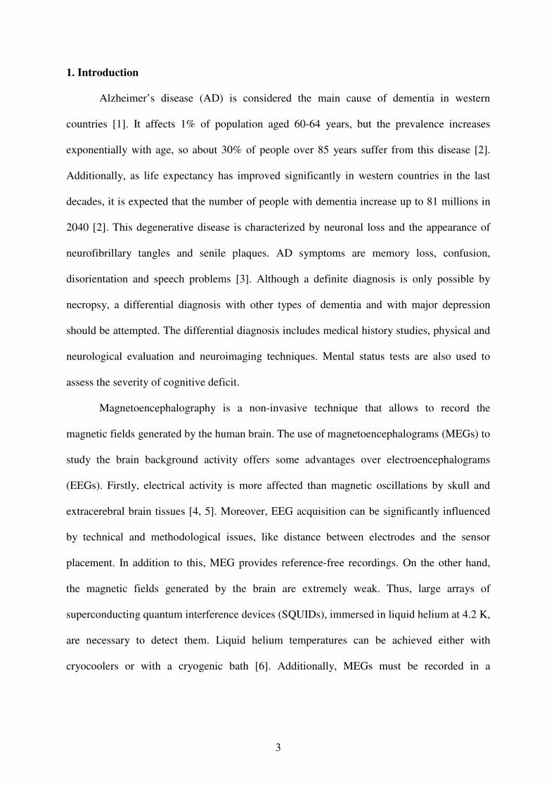
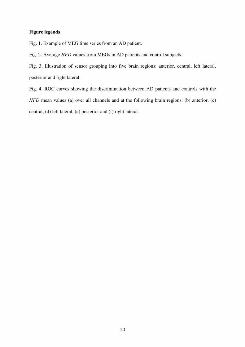
line analysis. Fig. 1 shows an example of an AD patient’s MEG epoch.

-----------------------------------------------------------------------------------------------------------------

INSERT FIGURE 1 AROUND HERE

-----------------------------------------------------------------------------------------------------------------

MEG data were acquired from 41 subjects: 20 patients with probable AD and 21

elderly control subjects. Cognitive status was screened in both groups with the Mini Mental

State Examination (MMSE) of Folstein et al. [32]. The AD group consisted of 20 patients (7

men and 13 women; age = 73.05 ± 8.65 years, mean ± standard deviation, SD) fulfilling the

criteria of probable AD, according to the criteria of the National Institute of Neurological and

Communicative Disorders and Stroke - Alzheimer’s and Related Disorders Association

(NINCDS-ADRDA). The mean MMSE score for the patients was 17.85 ± 3.91 points.

Patients were free of other significant medical, neurological and psychiatric diseases than AD.

Moreover, none of the participants in the study used medication that could affect the MEG

activity.

7

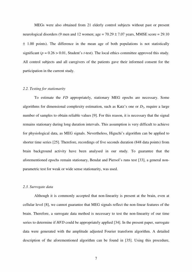
MEGs were also obtained from 21 elderly control subjects without past or present

neurological disorders (9 men and 12 women; age = 70.29 ± 7.07 years, MMSE score = 29.10

± 1.00 points). The difference in the mean age of both populations is not statistically

significant (p = 0.26 > 0.01, Student’s t-test). The local ethics committee approved this study.

All control subjects and all caregivers of the patients gave their informed consent for the

participation in the current study.

2.2. Testing for stationarity

To estimate the FD appropriately, stationary MEG epochs are necessary. Some

algorithms for dimensional complexity estimation, such as Katz’s one or D2, require a large

number of samples to obtain reliable values [9]. For this reason, it is necessary that the signal

remains stationary during long duration intervals. This assumption is very difficult to achieve

for physiological data, as MEG signals. Nevertheless, Higuchi’s algorithm can be applied to

shorter time series [25]. Therefore, recordings of five seconds duration (848 data points) from

brain background activity have been analysed in our study. To guarantee that the

aforementioned epochs remain stationary, Bendat and Piersol’s runs test [33], a general non-

parametric test for weak or wide sense stationarity, was used.

2.3. Surrogate data

Although it is commonly accepted that non-linearity is present at the brain, even at

cellular level [8], we cannot guarantee that MEG signals reflect the non-linear features of the

brain. Therefore, a surrogate data method is necessary to test the non-linearity of our time

series to determine if HFD could be appropriately applied [34]. In the present paper, surrogate

data were generated with the amplitude adjusted Fourier transform algorithm. A detailed

description of the aforementioned algorithm can be found in [35]. Using this procedure,

8

original and surrogate data have the same amplitude distribution and Fourier power spectra

[35]. Hence, surrogate data have the same linear properties than the original recordings, but

not the possible non-linear ones. Significant differences between the HFD values obtained

from the two data sets indicate that the signals are non-linear [36].

2.4. Higuchi’s fractal dimension (HFD)

Higuchi proposed in 1988 an efficient algorithm for measuring the FD of discrete time

sequences [25]. Higuchi’s algorithm calculates the FD directly from time series. As the

reconstruction of the attractor phase space is not necessary, this algorithm is simpler and

faster than D2 and other classical measures derived from chaos theory. FD can be used to

quantify the complexity and self-similarity of a signal [9]. HFD has already been used to

analyse the complexity of brain recordings [9, 37] and other biological signals [34, 38].

Given a one dimensional time series X = x[1], x[2],..., x[N], the algorithm to compute

the HFD can be described as follows [25]:

1. Form k new time series mkX defined by:

[ ] [ ] [ ]

⋅

−+++= k

k

mNmxkmxkmxmxX

mk int,...,2,,

where k and m are integers, and int(●) is the integer part of ●. k indicates the discrete

time interval between points, whereas m = 1, 2,..., k represents the initial time value.

2. The length of each new time series can be defined as follows:

( )

[ ] ( )[ ]

k

kk

mN

Nkimxikmx

kmL

k

mN

i

⋅

−

−

⋅−+−+

=

∑

−

= int

11

,

int

1

where N is length of the original time series X and ( ) ( )[ ]{ }kkmNN ⋅−− int1 is a

normalization factor.

9

3. Then, the length of the curve for the time interval k is defined as the average of the k

values L(m,k), for m = 1, 2, …, k:

( )∑=

⋅=k

m

kmLk

kL1

,1

)(

4. Finally, when L(k) is plotted against 1/k on a double logarithmic scale, with k = 1,

2,...,kmax, the data should fall on a straight line, with a slope equal to the FD of X.

Thus, HFD is defined as the slope of the line that fits the pairs ( )[ ] ( ){ }kkL /1ln,ln in a

least-squares sense. In order to choose an appropriate value of the parameter kmax,

HFD values were plotted against a range of kmax. The point at which the FD plateaus is

considered a saturation point and that kmax value should be selected [34, 39]. A value

of kmax = 48 was chosen for our study.

3. Results

Before the analysis of the recordings with HFD, the stationarity of the MEG epochs

was investigated using the Bendat and Piersol’s runs test [33]. The assessment of stationarity

with this method depends on the window length [40], a parameter that can be determined

estimating the dominant low frequency band in terms of energy distribution [41]. We found

that 72% of the MEG epochs retained the majority of the signal energy below 10.6 Hz. Thus,

a window of at least 94.3 ms is necessary. As a conservative estimate, the window length

should be more than three times this value [41]. Thus, in our study, a window of 300 ms, i.e.

50 samples, was employed. Using the aforementioned test, we found that 59.53% of the

epochs were stationary. These epochs were selected for further analysis with HFD and the

remainders were discarded.

A surrogate data method was used to detect the non-linearity in the MEGs. To

generate these artificial data, the amplitude adjusted Fourier transform algorithm [35] was

10

chosen. Our results showed statistically significant differences (p < 0.01, Student’s t-test)

between the HFD values obtained from the original and the surrogate data sets. Thus, we can

assume that the MEG time series used in our study contain non-linear features. These results

confirm the suitability of MEG analysis with HFD.

After testing the stationarity and non-linearity of the recordings, Higuchi’s algorithm

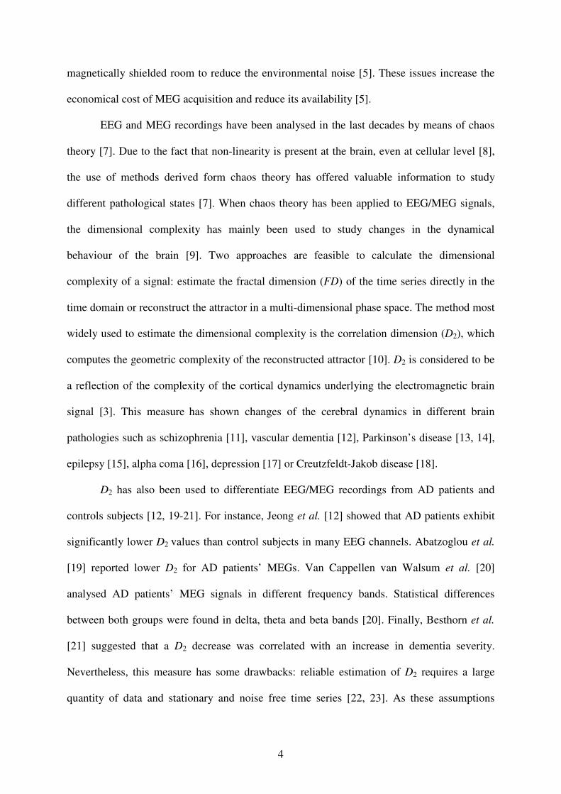
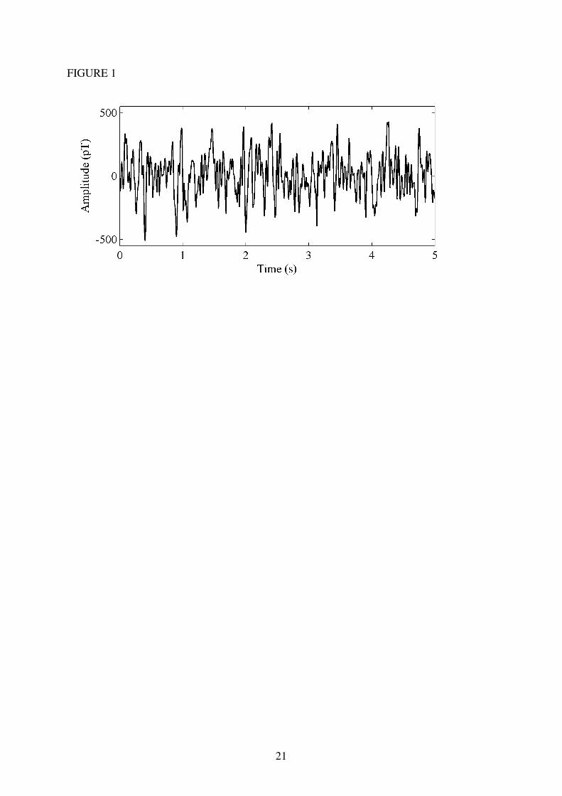
was applied. The average HFD value for the control group was 1.89 ± 0.03 (mean ± SD),

whereas it reached 1.81 ± 0.07 for AD patients. Our results showed that FD values were

higher in the control group than in the AD group for all channels (Fig. 2), which suggests that

AD is accompanied by a MEG complexity decrease. Additionally, differences between AD

patients and elderly control subjects were statistically significant in 71 channels (p < 0.01,

Student’s t-test with Bonferroni’s correction), specially in the temporal regions.

-----------------------------------------------------------------------------------------------------------------

INSERT FIGURE 2 AROUND HERE

-----------------------------------------------------------------------------------------------------------------

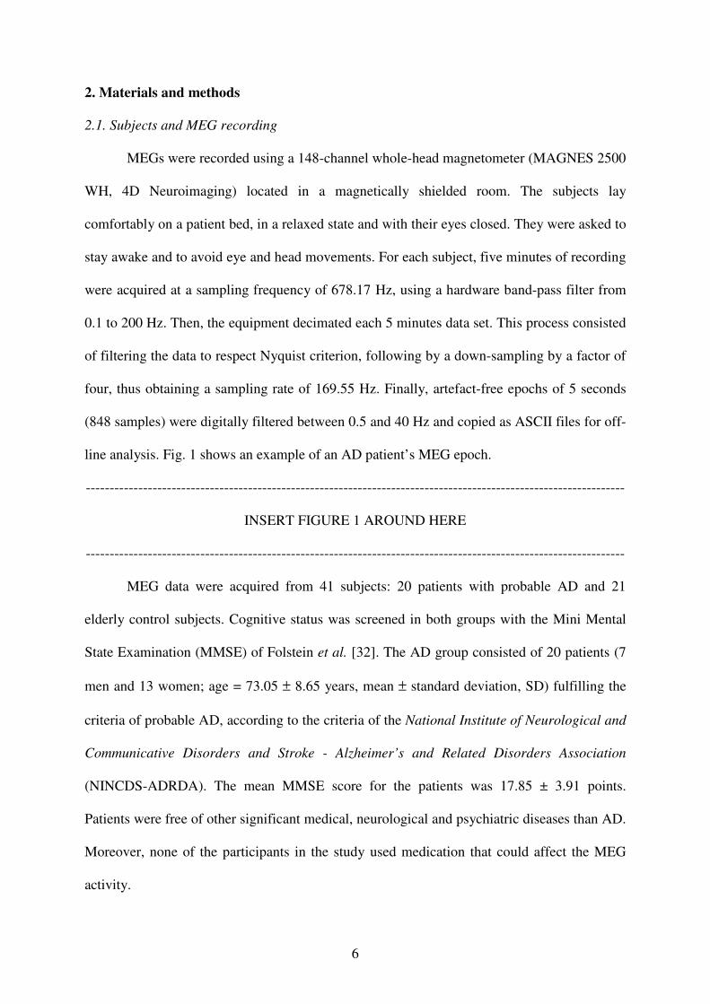
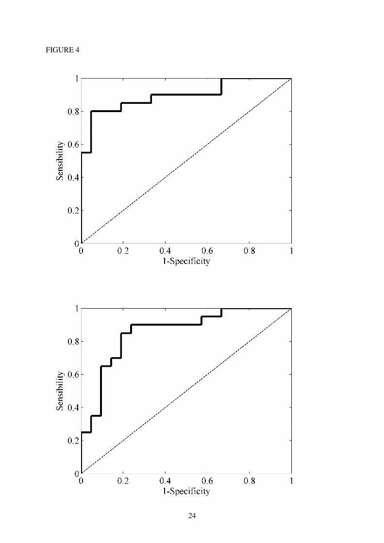
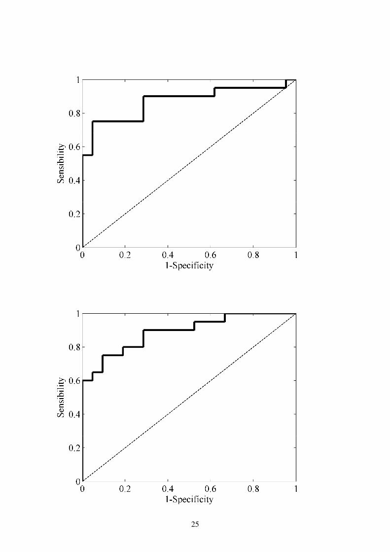
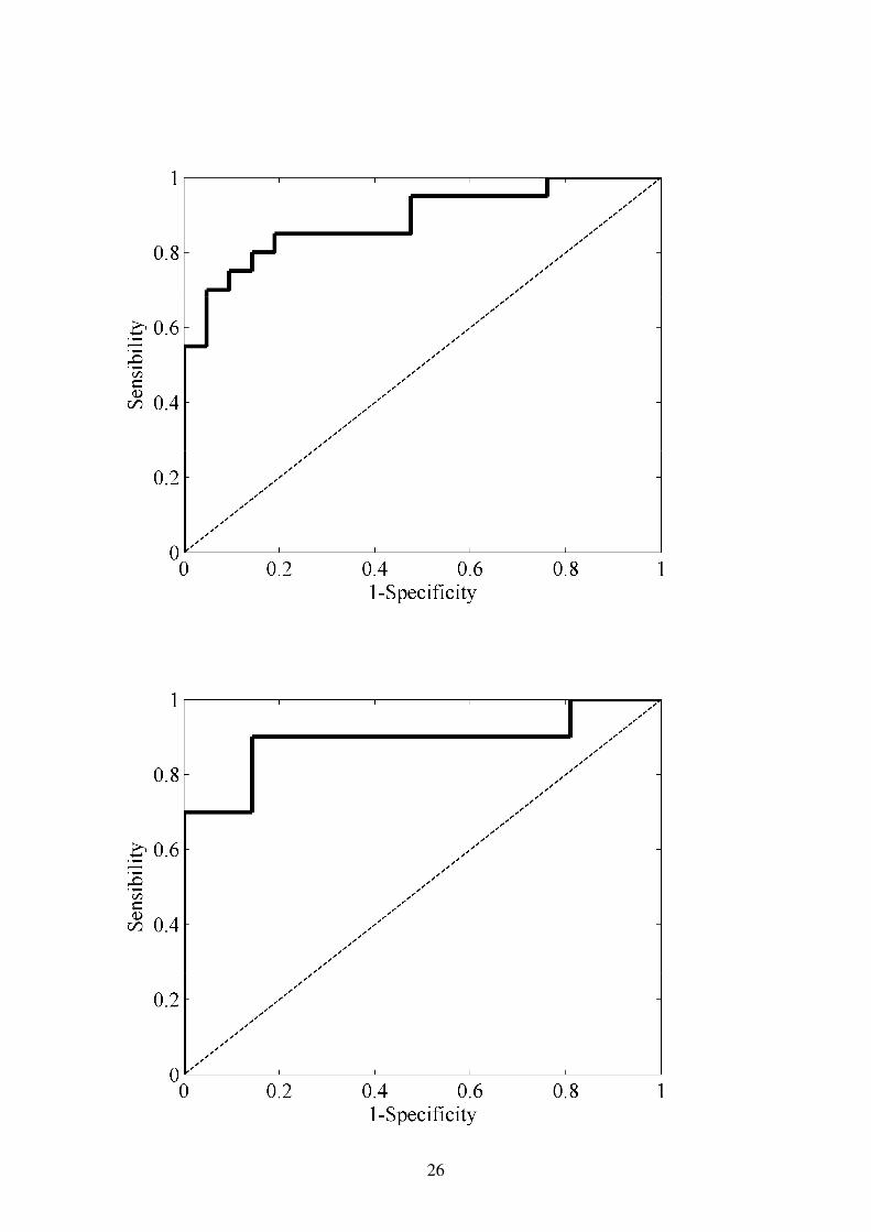
Furthermore, we evaluated the ability of HFD to discriminate AD patients from

elderly control subjects by means of receiver operating characteristic (ROC) curves. A ROC

curve is a graphical representation of the trade-offs between sensitivity and specificity. We

define sensitivity as the rate of AD patients who test positive, whereas specificity represents

the fraction of controls correctly recognized. Accuracy quantifies the total number of subjects

precisely classified. The area under the ROC curve (AROC) is a single number summarizing

the performance. AROC indicates the probability that a randomly selected AD patient has a

HFD value lower than a randomly chosen control subject. In order to calculate these values, a

leave-one-out cross-validation procedure was used. In the leave-one-out method, the results

from one subject are excluded from the training set one at a time. Afterwards, the results of

this subject are classified on the basis of the threshold calculated from the results obtained

11

from all other subjects. The leave-one-out cross-validation procedure provides a nearly

unbiased estimate of the true error rate of the classification procedure [42]. To simplify the

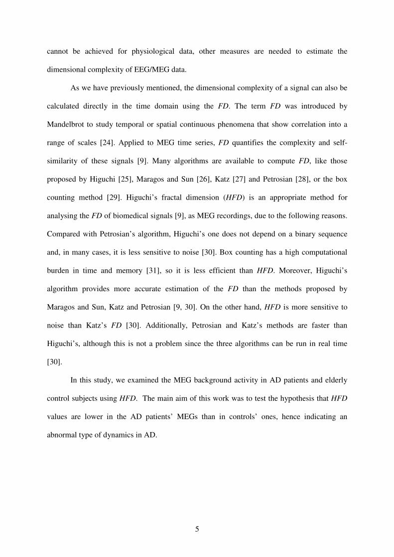
analyses, the HFD results were averaged over all channels. We also grouped the channels in

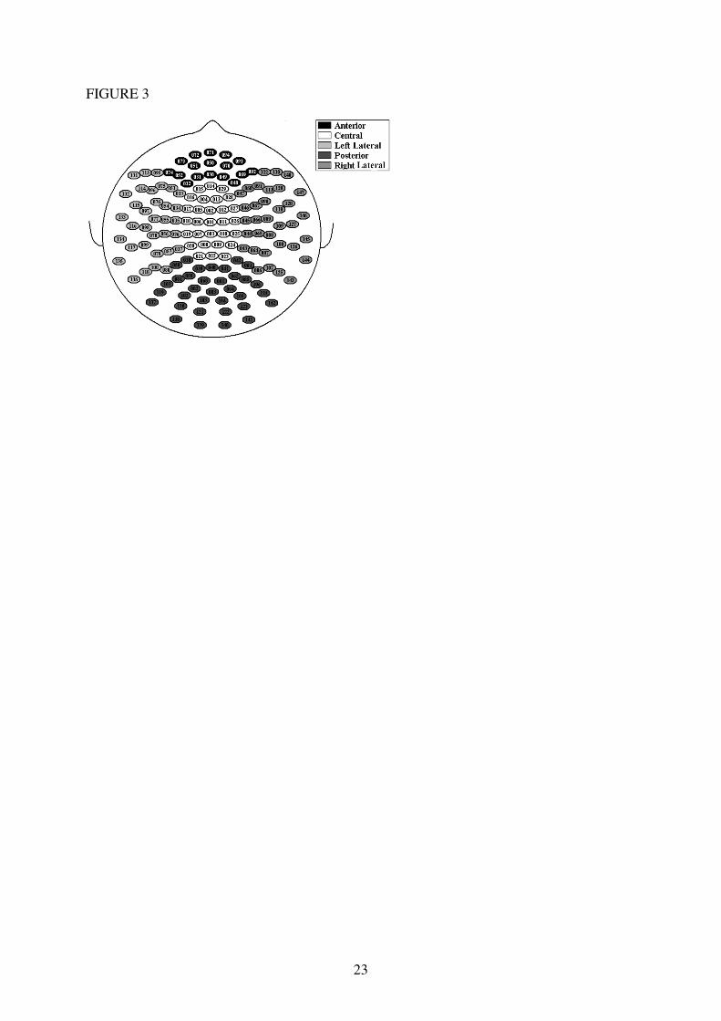
five brain areas (anterior, central, left lateral, posterior and right lateral), as Fig. 3 shows. Fig.

4 represents the ROC curves obtained at each region. The highest accuracy (87.8%) and

AROC (0.8952) values were achieved when the mean HFD over all channels was analysed.

Table 1 shows the sensitivity, specificity and accuracy values obtained at each region. The

AROC values and their 95% confidence intervals (CIs) are also presented.

-----------------------------------------------------------------------------------------------------------------

INSERT FIGURES 3 AND 4 AROUND HERE

-----------------------------------------------------------------------------------------------------------------

INSERT TABLE 1 AROUND HERE

-----------------------------------------------------------------------------------------------------------------

4. Discussion and conclusions

We explored the ability of HFD to discriminate between spontaneous MEG rhythms

of 20 AD patients and 21 control subjects. Before the complexity analysis with HFD, the

stationarity and the non-linear structure of the recordings were tested.

HFD has proven to be effective in discriminating AD patients from elderly controls.

Values were lower in AD patients at all MEG channels. Given the fact that FD can be used to

quantify the signal complexity [9], our study suggests that brains affected by AD show a less

complex behaviour. Additionally, the differences between both groups were statistically

significant in 71 channels (p < 0.01; Student’s t-test with Bonferroni’s correction). Our results

agree with previous studies that have analysed electromagnetic brain recordings with different

complexity measures. For instance, Jeong et al. [43] demonstrated that D2 values, calculated

12

from EEG, were significantly lower in AD patients than in controls. These results were

confirmed by Jelles et al. [10]. Abatzoglou et al. [19] showed that AD is associated with a

decrease in the dimensional complexity of MEG activity. Nevertheless, other MEG study

found that the variations reflected by D2 were in opposite directions in different frequency

bands [20]. Besthorn et al. [21] suggested that the dimensional complexity reduction is

correlated with the severity dementia. In other research work, EEGs obtained from probable

AD patients, autopsy-confirmed AD patients and controls were analysed by means of FD

[44]. Significant differences were found between the AD groups and the control group, and

also between probable and autopsy-confirmed patients [44]. Finally, Lempel-Ziv complexity

provided lower values in AD patients’ MEGs [45]. This complexity decrease may be due to

two cerebral mechanisms: a general effect of neurotransmitter deficiency and connectivity

loss of local neural networks as a result of nerve cell death [10].

The mean HFD values averaged over all channels were analysed by means of a ROC

curve, using a leave-one-out cross-validation procedure. An accuracy of 87.8% (80%

sensitivity; 95.24% specificity) was reached. Additionally, we explored the ability of HFD to

classify the MEGs from AD patients and controls at five brain areas (anterior, central, left

lateral, posterior and right lateral). In previous papers, non-linear methods and ROC curves

have been employed to classify MEG signals from AD patients and control subjects. For

instance, an accuracy of 83.3% was obtained with Lempel-Ziv complexity [45]. The accuracy

was slightly lower (82.9%) when the auto-mutual information decrease rate was analyzed

[46]. Despite the highest precision was achieved with HFD, all these values should be taken

with caution due to the small sample sizes.

Some limitations of our study merit consideration. Firstly, the sample size is small. To

prove the usefulness of HFD as a diagnostic tool, this approach should be extended on a

larger patient population before any conclusion can be made of its clinical diagnostic value.

13

Moreover, the detected decreased in complexity is not specific to AD and it appears in other

neurodegenerative diseases. Future efforts will be addressed to characterize the MEG

background activity in AD and in other types of dementia. Additionally, the results obtained

were averaged grouping the sensors in five brain areas to simplify the analyses. This issue

involves a loss of spatial information. Finally, Higuchi’s algorithm requires stationary MEG

epochs to estimate the FD appropriately. However, HFD may be a suitable method to analyse

physiological signals, since it can be applied to relatively short time series.

In summary, non-linear analysis of the MEG background activity with HFD showed a

decrease in the dimensional complexity of AD patients’ MEGs. The differences between AD

patients and elderly control subjects were statistically significant in 71 channels. Our findings

suggest that neuronal dysfunction in AD is associated with a decrease dimensional complexity

in MEG signals.

Acknowledgements

This work has been supported in part by “Consejería de Educación de la Junta de

Castilla y León” under projects VA108A06 and VA102A06. The authors would like to thank

the “Asociación de Familiares de Enfermos de Alzheimer” in Madrid (Spain) for supplying

the patients who took part in this study.

14

References

[1] Bird TD. Alzheimer’s disease and other primary dementias. In: Braunwald E, Fauci AS,

Kasper DL, Hauser SL, Longo DL, Jameson JL, editors. ‘Harrison's Principles of

Internal Medicine’. New York: The McGraw-Hill Companies Inc., 2001:2391–9.

[2] Jorm AF. Cross-national comparisons of the occurrence of Alzheimer’s and vascular

dementias. Eur Arch Psychiatry Clin Neurosci 1991;240:218–22.

[3] Jeong J. EEG dynamics in patients with Alzheimer’s disease. Clin Neurophysiol

2004;115:1490–505.

[4] Hämäläinen M, Hari R, Ilmoniemi RJ, Knuutila J, Lounasmaa OV.

Magnetoencephalography – theory, instrumentation, and applications to noninvasive

studies of the working human brain. Rev Mod Phys 1993;65:413–97.

[5] Hari R. Magnetoencephalography in clinical neurophysiological assessment of human

cortical functions. In: Niedermeyer E, Lopes da Silva F, editors.

‘Electroencephalography: basic principles, clinical applications, and related fields’.

Philadelphia: Lippincontt Williams & Wilkins, 2005:1165–97.

[6] Jiri V, Robinson E. Signal processing in magnetoencephalography. Methods

2001;25:249–71.

[7] Stam CJ. Nonlinear dynamical analysis of EEG and MEG: review of an emerging field.

Clin Neurophysiol 2005;116:2266–301.

[8] Andrzejak RG, Lehnertz K, Mormann F, Rieke C, David P, Elger CE. Indications of

nonlinear deterministic and finite-dimensional structures in time series of brain

electrical activity: Dependence on recording region and brain state. Phys Rev E

2001;64:061907.

15

[9] Accardo A, Affinito M, Carrozzi M, Bouquet F. Use of fractal dimension for the

analysis of electroencephalographic time series. Biol Cybern 1997;77:339-50.

[10] Jelles B, van Birgelen JH, Slaets JPJ, Hekster REM, Jonkman EJ, Stam CJ. Decrease of

non-linear structure in the EEG of Alzheimer patients compared to healthy controls.

Clin Neurophysiol 1999;110:1159–67.

[11] Kotini A, Anninos P. Detection of non-linearity in schizophrenic patients using

magnetoencephalography. Brain Topogr 2002;15:107–13.

[12] Jeong J, Chae JH, Kim SY, Han SH. Nonlinear dynamic analysis of the EEG in patients

with Alzheimer’s disease and vascular dementia. J Clin Neurophysiol 2001;18:58–67.

[13] Anninos PA, Adamopoulos AV, Kotini A, Tsagas N. Nonlinear analysis of brain

activity in magnetic influenced Parkinson patients. Brain Topogr 2000;13:135–44.

[14] Stam CJ, Jelles B, Achtereekte HAM, Rombouts SARB, Slaets JPJ, Keunen RWM.

Investigation of EEG nonlinearity in dementia and Parkinson's disease. Electroenceph

Clin Neurophysiol 1995;95:309–17.

[15] Hornero R, Espino P, Alonso A, López M. Estimating complexity from EEG

background activity of epileptic patients. IEEE Eng Med Biol 1999;18:73–79.

[16] Kim YW, Krieble KK, Kim CB, Reed J, Rae-Grant AD. Differentiation of alpha coma

from awake alpha by nonlinear dynamics of electroencephalography. Electroenceph

Clin Neurophysiol 1996;98:35–41.

[17] Nandrino JL, Pezard L, Martinerie J, el Massioui F, Renault B, Jouvent R, Allilaire JF,

Wildlöcher D. Decrease of complexity in EEG as a symptom of depression.

NeuroReport 1994;5:528–30.

16

[18] Babloyantz A, Destexhe A. The Creutzfeldt-Jakob disease in the hierarchy of chaotic

attractors. In: Markus M, Müller S, Nicolis G, editors. ‘From chemical to biological

organization’. Berlin: Springer-Verlag, 1988:307–16.

[19] Abatzoglou I, Anninos P, Adamopoulos A, Koukourakis M. Nonlinear analysis of brain

magnetoencephalographic activity in Alzheimer disease patients. Acta Neurol Belg

2007;107:34–9.

[20] van Cappellen van Walsum AM, Pijnenburg YAL, Berendse HW, van Dijk BW, Knol

DL, Scheltens Ph, Stam CJ. A neural complexity measure applied to MEG data in

Alzheimer’s disease. Clin Neurophysiol 2003;114:1034–40.

[21] Besthorn C, Sattel H, Geiger-Kabisch C, Zerfass R, Förstl H. Parameters of EEG

dimensional complexity in Alzheimer’s disease. Electroenceph Clin Neurophysiol

1995;95:84–9.

[22] Eckmann JP, Ruelle D. Fundamental limitations for estimating dimensions and

Lyapunov exponents in dynamical systems. Physica D 1992;56:185–7.

[23] Grassberger P, Procaccia I. Characterization of strange attractors. Phys Rev Lett

1983;50:346–9.

[24] Mandelbrot BB. How long is the coast of Britain? Statistical selfsimilarity and

fractional dimension. Science 1967;156:636–8.

[25] Higuchi T. Approach to an irregular time series on the basis of the fractal theory.

Physica D 1988;31:277–83.

[26] Maragos P, Sun FK. Measuring the fractal dimension of signals: morphological covers

and iterative optimization. IEEE Trans Signal Proc 1983;41:108–21.

[27] Katz M. Fractals and the analysis of waveforms. Comput Biol Med 1988;18:145–56.

17

[28] Petrosian A. Kolmogorov complexity of finite sequences and recognition of different

preictal EEG patterns. Proc IEEE Symp Computer-Based Med Syst 1995:212–17.

[29] Mandelbrot B. Fractals: Form, Chance, and Dimension. San Francisco: Freeman, 1977.

[30] Esteller R, Vachtsevanos G, Echauz J, Litt B. A comparison of waveform fractal

dimension algorithms. IEEE Trans Circuits Syst 2001;48:177–83.

[31] Block A, von Bloh W, Schellnhuber HJ. Efficient box-counting determination of

generalized fractal dimensions. Phys Rev A 1990;42:1869–74.

[32] Folstein MF, Folstein SE, McHugh PR. Mini-mental state. A practical method for

grading the cognitive state of patients for the clinician. J Psychiatr Res 1975;12:189–98.

[33] Bendat J, Piersol A. Random data: analysis and measurement procedures. New York:

Willey, 2000.

[34] Doyle TLA, Dugan EL, Humphries B, Newton RU. Discriminating between elderly and

young using a fractal dimension analysis of centre of pressure. Int J Med Sci 2004;1:11–

20.

[35] Theiler J, Eubank S, Longtin A, Galdrikian B, Doyne Farmer J. Testing for nonlinearity

in time series: the method of surrogate data. Physica D 1992;58:77–94.

[36] Timmer J. Power of surrogate data testing with respect to nonstationarity. Phys Rev E

1998;58:5153–56.

[37] Ferenets R, Lipping T, Anier A, Jäntti V, Melto S, Hovilehto S. Comparison of entropy

and complexity measures for the assessment of depth of sedation. IEEE Trans Biomed

Eng 2006;53:1067–77.

[38] Acharya R, Bhat PS, Kannathal N, Rao A, Lim CM. Analysis of cardiac health using

fractal dimension and wavelet transformation. ITBM-RBM 2005;26:133–9.

18

[39] Klonowsky W, Olejarczyk E, Stepien R. Epileptic seizures in economic organism.

Physica A 2004;342:701–7.

[40] Duchene J, Goubel F. Surface electromyogram during voluntary contractions:

Processing tools and relation to physiological events. Crit Rev Biomed Eng

1993;21:313–97.

[41] Chau T, Chau D, Casas M, Berall G, Kenny DJ. Investigating the stationarity of

paediatric aspiration signals. IEEE Trans Neural Syst Rehab Eng 2005;13:99–105.

[42] Simon R, Radmacher MD, Dobbin K, McShane KM. Pitfalls in the use of DNA

microarray data for diagnostic and prognostic classification. J Natl Cancer Inst

2003;95:14–8.

[43] Jeong J, Kim SJ, Han SH. Non-linear dynamical analysis of the EEG in Alzheimer’s

disease with optimal embedding dimension. Electroencephalogr Clin Neurophysiol

1998;106:220–8.

[44] Woyshville MJ, Calabrese JR. Quantification of occipital EEG changes in Alzheimer's

disease utilizing a new metric: the fractal dimension. Biol Psychiatry 1994;35:381–7.

[45] Gómez C, Hornero R, Abásolo D, Fernández A, López M. Complexity analysis of the

magnetoencephalogram background activity in Alzheimer’s disease patients. Med Eng

Phys 2006;28:851–9.

[46] Gómez C, Hornero R, Abásolo D, Fernández A, Escudero J. Analysis of the

magnetoencephalogram background activity in Alzheimer’s disease patients with auto-

mutual information. Comput Meth Programs Biomed 2007;87:239–47.

19

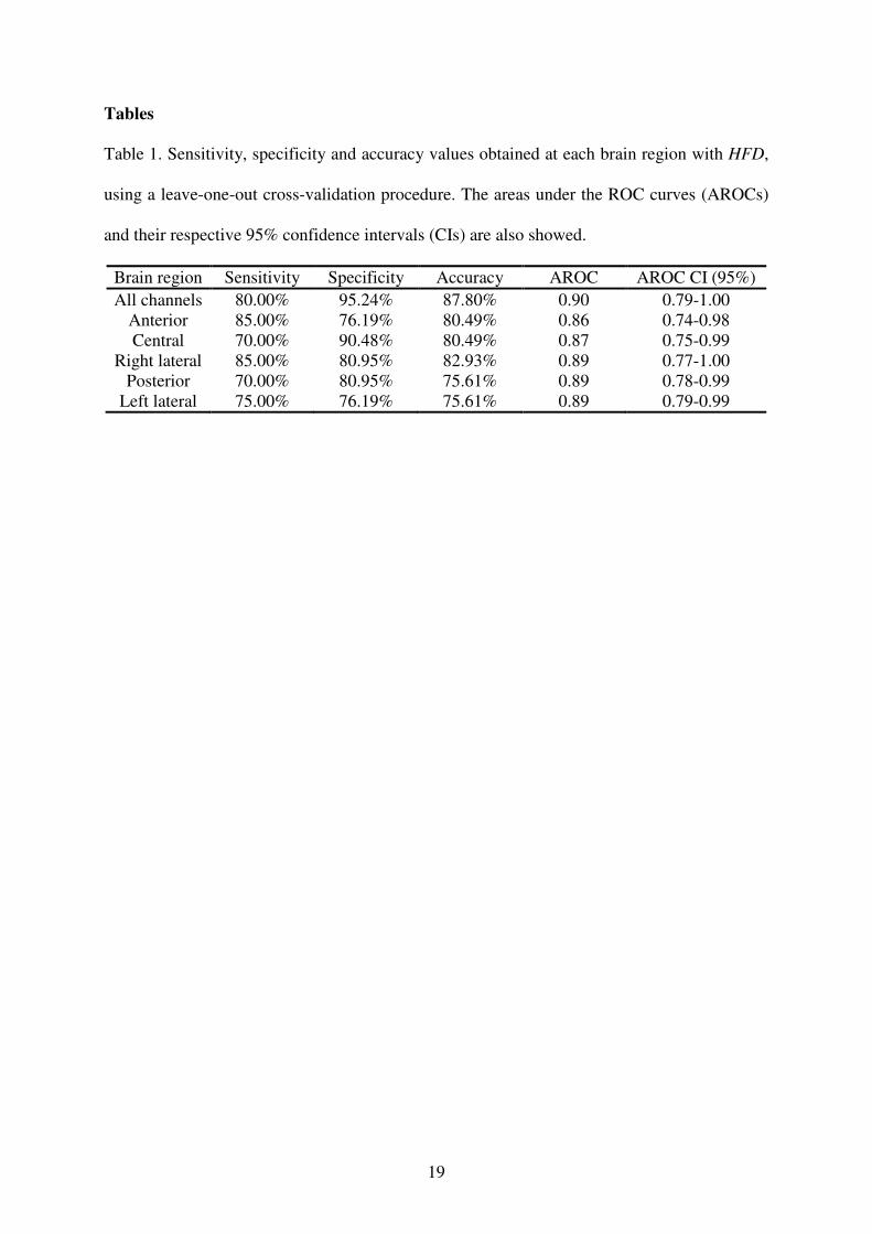
Tables

Table 1. Sensitivity, specificity and accuracy values obtained at each brain region with HFD,

using a leave-one-out cross-validation procedure. The areas under the ROC curves (AROCs)

and their respective 95% confidence intervals (CIs) are also showed.

Brain region Sensitivity Specificity Accuracy AROC AROC CI (95%) All channels 80.00% 95.24% 87.80% 0.90 0.79-1.00

Anterior 85.00% 76.19% 80.49% 0.86 0.74-0.98 Central 70.00% 90.48% 80.49% 0.87 0.75-0.99

Right lateral 85.00% 80.95% 82.93% 0.89 0.77-1.00 Posterior 70.00% 80.95% 75.61% 0.89 0.78-0.99

Left lateral 75.00% 76.19% 75.61% 0.89 0.79-0.99

20

Figure legends

Fig. 1. Example of MEG time series from an AD patient.

Fig. 2. Average HFD values from MEGs in AD patients and control subjects.

Fig. 3. Illustration of sensor grouping into five brain regions: anterior, central, left lateral,

posterior and right lateral.

Fig. 4. ROC curves showing the discrimination between AD patients and controls with the

HFD mean values (a) over all channels and at the following brain regions: (b) anterior, (c)

central, (d) left lateral, (e) posterior and (f) right lateral.

21

FIGURE 1

22

FIGURE 2

23

FIGURE 3

24

FIGURE 4

25

26