Use of Simulations in Determination of Wheel Impact Forces

Yan Sun Use of Simulations in Determination of Wheel CRE, CQ University Impact Forces P1 and P2 Due to Rail Dip Defects

AusRAIL 2009 17-19 November 2009, Australia

Use of Simulations in Determination of Wheel Impact Forces P1 and P2 Due to

Rail Dip Defects

Yan Quan Sun1, Colin Cole

1, Malcolm Kerr

2 & Sak Kaewunruen

2

1Centre for Railway Engineering, CQ University, Australia

Email: [email protected]; Tel: 07 49309287 2RailCorp, NSW

Abstract A rail vehicle-track interaction dynamics model has been applied to determine the track vertical dynamic forces due to rail dip defects such as dip joints and welds, which are required in railway vehicle acceptance procedure. The model was validated using the field measurement data of rail dip defects and accelerations of a vehicle axlebox. The simulated dynamic forces – the P2 forces have been compared with those calculated using a well-known formula. Their difference and the formula’s limitation have been discussed. The effects of the rail dip defect and the vehicle speed on the track vertical dynamic force have also been investigated.

1. Introduction

The field testing for the determination of railway track vertical dynamic forces, as one of railway vehicle acceptance procedures, would be expensive, complex and time consuming. Alternatively, the use of some formulas to calculate these forces could cause the errors. The advanced simulation techniques can improve this and can be taken as a substitution of test work or simple calculation. In this case, significant savings of time and money and, more importantly, safety is not compromised. When rail vehicles run over a track with rail dip defects such as dipped weld joints, the dynamic forces generated on the wheel-rail interface inevitably cause deterioration and damage to the track. As a result, the push for higher axle load and faster trains risks more adverse maintenance and safety outcomes. Safe operation of vehicle and track system requires that the maximum permissible force levels are clearly defined and reasonably determined. As one of the limits, the maximum permissible P2 force levels have been stipulated by many railway authorities to restrict access of new vehicles into network, e.g. P2 < 200kN for a vehicle running through a dip angle with 0.01 radian at its nominal maximum speed and nominal gross mass for interstate network in Australia. Forces P1 and P2 were originally used by Jenkins et al [1] to term the peak values of track vertical dynamic forces (or wheel dynamic forces), which occur when a wheel travels across a classical dipped rail joint, or a dipped weld joint. The P1 force is a very high frequency (>>100 Hz) force, which is superimposed on P2 force and is due to the inertia of the rail. Its effects are largely limited to rail surface failure. The P2 force occurs at a lower frequency (30 ~ 90 Hz) than the P1 force. The P2 force is principally responsible for causing the unsprung mass and the rail/sleeper mass to move down together,

causing concrete sleeper breakage and ballast hardening. For this reason, P2 is of great interest to the railway operators. The following formula, Eq. (1) is widely used to calculate P2:

(1)

Where P0 is the static wheel load (kN), Mu is the vehicle unsprung mass (kg), 2α is the total dip joint angle (rad), V is the speed of vehicle (m/s), Kt is the equivalent track stiffness (MN/m), Ct is the equivalent track damping (kNs/m) and Mt is the equivalent track mass (kg). The current P2 force formula is not without limitations and further investigations are required to consider the following:

• The inadequate definition of unsprung mass. P2 would be least accurately calculated for widely used three-piece bogie wagons due to wedge friction in secondary suspension.

• The non-linear relationship between P2 and dip joint angle.

• The non-linear relationship between P2 and travel speed.

• The relationship between P2, track equivalent stiffness, damping and mass parameters.

• The selection or calculation of track equivalent stiffness, damping and mass, e.g. Kt = 109 MN/m, Ct = 52 kNs/m and Mt = 133 kg as given in a procedure [11].

• The use of the same P2 limits for freight wagons and the application of P2 limits to higher speed.

• Ignorance of P1 limit. A cost-effective method to accurately determine the wheel dynamic forces (including P1 and P2 forces) is through simulation. Several theoretical simulation methods have been developed to determine the wheel



dynamic forces. A wheel/rail and track dynamic interaction model was developed by Cai [2] to calculate the wheel-rail impact forces. A similar model to that by Cai [2] was applied by Dahlberg [3] to investigate the effect of rail pads to the wheel dynamic forces. A vehicle-track model was used by Shen [4] to determine the wheel-rail vertical and lateral dynamic forces and the methods to reduce the dynamic forces were put forward. A finite element model of railway track was generated by Dong et al [5] to determine the wheel dynamic forces. Zarembski [6] provided a plot of the relationship between P1 and P2 with the unsprung mass, the track modulus and the track mass. The relationship between the geometry of rail welds and the dynamic wheel–rail response was obtained through numerical simulation by Steenbergen and Esveld [7] to assess the rail weld condition. A three dimensional vehicle–track coupled dynamics model was developed by Zhai et al [8] to investigate the dynamics of overall vehicle–track systems In this paper, a three-dimensional vehicle-track system dynamics model (Sun et al [9], [10]), simply called CRE-3DVTSD model, has been applied. The three translational and three rotational movements of all rail vehicle components – vehicle car body, two bolsters, two sideframes and four wheelsets were considered. The track model employed a discretely supported distributed parameter system with one layer. The simulation results have been validated using the data of manually measured rail dip defects and the data of a vehicle axlebox acceleration measurement. Forces P1 and P2 have been determined through simulation. The comparison between the simulation results and the results using Eq. (1) are also presented and discussed. The railway vehicle acceptance procedures may then be structured around the simulated P2 force limits. 2. Railway Vehicle-Track Interaction Dynamics

Modelling

In this section, the vehicle-track modelling is illustrated and described. Our previous work on vehicle-track interaction dynamics (Sun et al (2001, 2007)) has given a full description of the differential equations. The modelling is deployed as in-house FORTRAN code. This section presents the vehicle-track modelling, the wheel-rail interface modelling, and the model validation. 2.1 Vehicle-Track Modelling Figure 1(a), 1(b), 1(c) and 1(d) show vehicle-track model called 3D-VTSD.

ICx

CZ

CY

CX

Czφ

Cyφ

Cxφ

Cw

Cv

Wagon Car Body

Front Bolster

Rear Bolster

1(a) A Vehicle Car Body and Two Bolsters

Right Rail

Wheelset

Bogie Structure

Bolster

BZ

BY

BXBcH

Primary Suspension

Secondary Suspension

1(b) Bogie

1(c) Track Longitudinal View

1(d) Track Lateral View

Figure 1 3D VTSD Model Representation The Vehicle model includes one car body, two bolsters, two sideframes, and four wheelsets. All components are modelled as rigid bodies with six degrees of freedom (DoF) (lateral, vertical and longitudinal displacements, and roll, pitch and yaw rotations). The vehicle car body, as shown in Figure 1(a), rests on two bolsters through two centre bowls, and is longitudinally connected with two couplers, which are represented as springs. Nonlinear connection characteristics such as vertical lift-off and lateral and longitudinal impacts between sideframe and wheelset, sideframe and bolster, and bolster and vehicle car body are fully considered. The track subsystem is considered as the discretely supported track with one layer as shown in Figure 1(c)



and 1(d). The track components are assembled exactly as the conventional ballasted track structure (e.g. sleeper spacing, pad and fastener stiffness, ballast modulus and depth, and subgrade modulus). The track model is structured as two Timoshenko beams, which represent two rails, supported by discretely distributed spring-damper elements, which represent the combined elasticity of rail pads and fasteners, ballast and subgrade. There are five DoFs at any point on the rail

beam – lateral and vertical displacements ( Riv and

Riw ( r,li = )), and three rotations ( Rixφ , Riyφ and

Rizφ ) about longitudinal, lateral and vertical directions.

Equivalent stiffness and damping coefficients have been used to take into account the stiffness and damping of rail pad, sleeper and ballast. In this track model, the effect of sleeper and ballast masses has been ignored. For simplicity, the dynamic equilibrium equations of the rail beam have been expanded using a Fourier series in

the longitudinal ( X ) direction by assigning an equal

number of terms ( mn , also known as the number of

modes of the rail beam) for both the linear displacements and the angular rotations. 2.2 Wheel-Rail Interface Modelling For the wheel-rail interface, the normal force due to wheel-rail rolling contact is determined using Hertz static contact theory. The tangent creep forces and the creep moments are defined using Kalker’s linear creep theory. The comprehensive model includes the vertical and lateral velocities of the rail in the definition of the creepages in the lateral and spin directions. The normal

contact force WTnF is determined using Hertz contact

theory and can be expressed in Eq. (2):

[ ]

<µ−−

>µ−−µ−−=

0)x(wwif0

0)x(wwif)x(wwCF

wR

wR

2/3

wRHWTn

(2)

where HC is Hertz contact coefficient, Rw and ww

are the vertical displacements of rail and wheel at the

contact point, and )x(µ is the function representing the

wheel or rail defects. 2.3 Solution Technique For the vehicle model the equations of dynamic equilibrium may be written using multi-body mechanics methods. For the track model the lateral and the vertical bending and shear deformations of the rail are described using Timoshenko beam theory in addition to considering the torque of the rail beam. After applying a Fourier series expansion in the longitudinal direction, the equations of dynamic equilibrium were obtained for the rails. The equations of dynamic equilibrium for wagon and track modelling are expressed in Eq. (3):

=

+

+

WT

WT

T

W

T

W

T

W

T

W

T

W

T

W

F

F

d

d

K

K

d

d

C

C

d

dM~

0

0

0

0

M0

0

&

&

&&

&&

(3)

Where WM and TM , WC and

TC , and WK and

TK are the mass, damping and stiffness matrices of

wagon/track modelling. Parameter Wd is the

displacement vector of the wagon subsystem, and

vector Td contains displacement of the track

subsystem that includes the modal and physical

displacements. Parameter WTF is the wheel-rail

interface force vector consisting of the wheel-rail normal contact forces, tangent creep forces and creep moments about the normal direction in the wheel-rail contact

plane. Parameter WTF~

is the combined wheel-rail

interface force vector. A modified Newmark β− method

is employed to solve Eq. (3). 2.4 Modelling Validation In a selected track line, it was found that there were a number of rail top defects throughout the site, associated with the dipped welds, squats and top defects due to fouled ballast. Figure 2(a) and 2(b) illustrate two squats defects, and their measurements using a 1.0 metre dip gauge are presented in Figure 2(c) and 2(d).

2(a) #1 Squat Defect

2(b) #2 Squat Defect



2(c) Profile Corresponding to #1 Defect

2(d) Profile Corresponding to #2 Defect

Figure 2 Single Dip Measured Profiles When a rail vehicle (its parameter data is given in Appendix-I) passed through these two defect locations, significant wheel impacts were generated. The accelerometers were installed on the axle boxes (Figure 3(a)), from which the impact accelerations were recorded as shown in Figure 3(b).

3(a) Accelerometers

3(b) Acceleration data

Figure 3 Acceleration Measurements Figure 4 compares the measured results with the results from the 3D VTSD model simulations.

4(a) Measured Acceleration due to #1 Defect

4(b) Simulated Acceleration due to #1 Defect

4(c) Dip defect and Wheel displacement due to #1

Defect

4(d) Measured Acceleration due to #2 Defect



4(e) Simulated Acceleration due to #2 Defect

4(f) Dip defect and Wheel displacement due to #2

Defect Figure 4 Measured and Simulated Results From the comparison of measured and simulated accelerations, it can be seen that the simulated results are in good agreement with the measured ones. For the larger dip defects as shown in Figure 2(b) and 2(d), the simulations indicated that after the wheel enters the defect, the wheel will separate with the rail and briefly fly over the rail, leading to a zero contact force. When the wheel lands on the rail, a larger wheel impact will be generated (Figure 4(d) and 4(e)). From the simulated wheel displacements shown in Figure 4(c) and 4(f), it is evident that the wheel cannot touch the bottom of these particular defects, as the wheel displacements cannot follow the defect profiles. 3. Application of the P2 Force Equation An example for the application of P2 force equation (Eq. (1)) is from the Rail Industry Safety and Standard Board (RISSB), Australia [11]. In its application, Kt is nominally taken as 109MN/m, Ct is 52kNs/m, and Mt is 133kg. From Eq. (1), it can be seen that P2 changes linearly with the static wheel load, the dip angle and the speed, and nonlinearly with the unsprung mass, the track parameters – equivalent stiffness, damping and mass. It can be also seen that the dip angle only affects P2 regardless of how large a dip defect is. According to [11], the P2 force exerted by rollingstock travelling at its nominal maximum speed and nominal gross mass over a dipped weld in one rail shall not exceed the limits set out in Table 1.

Table 1

Route Rail size

(kg/m) 0.010 rad dip 0.014 rad dip

Interstate standard gauge network > 53 200

Railcorp Class 1 track > 53 (192) 230

Railcorp Class 2 track < 53 (192) 230

1067mm gauge track > 41 200

Note: Figures in brackets are approximate figures scaled for 0.01 radian dip

P2 force limit (kN)

The unsprung mass is defined approximately as the mass between the rail and the bogie suspension. For the vehicle (its parameter data are given in Appendix-I), the effective unsprung mass is Mu = 1120 kg, and the static wheel load is P0 = 57.575 kN. 3.1 P2 Force via Speed V, Dip Angle α and

Unsprung Mass In this situation, the parameters are selected using the nominal values as shown below:

• Kt = 109MN/m

• Ct = 52kNs/m

• Mt = 133kg

• P0 = 57.575 kN Figure 5(a), 5(b) and 5(c) show the relationship between the calculated value of P2 & speed, P2 & dip angle, and P2 & unsprung mass.

5(a) P2 and Speed

5(b) P2 and Dip Angle



5(c) P2 and Unsprung Mass (at α = 0.01 radian)

Figure 5 Relationship between P2 and Speed, Dip Angle and Unsprung Mass It can be seen from Figure 5 that the P2 force increases as the speed, dip angle and the unsprung mass increase. For examples, in Figure 5(a) at α = 0.01 radian and when the speed changes from 60 km/h to 120 km/h (a 100% increase), the P2 force increases from 155.5 kN to 253.65 kN (a 63% increase). In Figure 5(b), at V = 100 km/h and when the dip angle increases from 0.006 to 0.012 (a 100% increase), the P2 force increases from 156 kN to 254.5 kN (a 63.7% increase). In Figure 5(c), at the conditions of α = 0.01 radian and V = 100 km/h, and when the unsprung mass increases from 800 kg to 1600 kg (a 100% increase), P2 increases from 190.3 kN to 258.6 kN (a 35.9% increase). It can be seen that the speed and the dip angle have a similar influence on the P2 force, and that this influence on P2 is much larger than that for the unsprung mass. 3.2 P2 and Track Parameters In this situation, the parameters are selected as below:

• α = 0.01 radian

• P0 = 57.575 kN

• Mu = 1120 kg Figure 6(a), 6(b) and 6(c) show the relationship between P2 and track parameters.

6(a) P2 and Track Mass

6(b) P2 and Track Damping

6(c) P2 and Track Stiffness

Figure 6 Relationship between P2 and Track Parameters It can be seen from Figure 6 that P2 decreases as the track mass and damping increase. However, P2 increases as the track stiffness increase. For example, in Figure 6(a), at the speed of 90 km/h and when the track mass increases from 100 kg to 200 kg (a 100% increase), the P2 force decreases from 206.3 kN to 201 kN (a 2.6% decrease). In Figure 6(b), at V = 90 km/h and when the track damping increases from 40 kNs/m to 80 kNs/m (a 100% increase), the P2 force decreases from 208.4 kN to 194.6 kN (a 6.6% decrease). In Figure 6(c), at V = 90 km/h, when the track stiffness increases from 80 MN/m to 160 MN/m (a 100% increase), P2 increases from 180 kN to 238.6 kN (a 32.6% increase). It can be said that the track mass and track damping do not significantly influence P2 compared with the track stiffness. 4. Simulations Using 3D VTSD Model 4.1 Rail Dip Modelling The rail dip defect model is well-known and illustrated in Figure 7 and expressed as Eq. (4).



Figure 7 Rail Dip Model where L is the dip length (m), D is the dip depth (mm) and α is the dip angle (radian). The rail joint dip can be expressed as:

+>

+≤≤+−

π+−

+<≤−

π−−

=µ

Lxx

LxxLxL

xxD

LxxxL

xxD

x

0

000

000

0

2/)]2

2cos(1[

2/)]2

2cos(1[

)(

(4) 4.2 Relation of P2 to Dip Angle

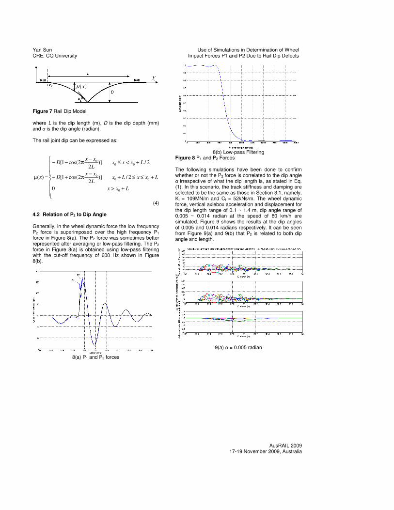
Generally, in the wheel dynamic force the low frequency P2 force is superimposed over the high frequency P1 force in Figure 8(a). The P2 force was sometimes better represented after averaging or low-pass filtering. The P2 force in Figure 8(a) is obtained using low-pass filtering with the cut-off frequency of 600 Hz shown in Figure 8(b).

8(a) P1 and P2 forces

8(b) Low-pass Filtering

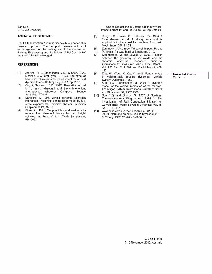
Figure 8 P1 and P2 Forces The following simulations have been done to confirm whether or not the P2 force is correlated to the dip angle α irrespective of what the dip length is, as stated in Eq. (1). In this scenario, the track stiffness and damping are selected to be the same as those in Section 3.1, namely, Kt = 109MN/m and Ct = 52kNs/m. The wheel dynamic force, vertical axlebox acceleration and displacement for the dip length range of 0.1 ~ 1.4 m, dip angle range of 0.005 ~ 0.014 radian at the speed of 80 km/h are simulated. Figure 9 shows the results at the dip angles of 0.005 and 0.014 radians respectively. It can be seen from Figure 9(a) and 9(b) that P2 is related to both dip angle and length.

9(a) α = 0.005 radian



9(b) α = 0.0075 radian

Figure 9 Dynamic Responses at Speed of 80 km/h Figure 10 shows the relationship between P2 and the dip length under the influence of the dip angle being 0.005, 0.0075, 0.01 and 0.014 radians.

Figure 10 Relationship between P2 and the Dip Length From Figure 10, it seems that for the dip length larger than 0.5m the P2 force remains constant for dip angle and independent of the dip length at the speed of 80 km/h. However, the dip length of 0.25m makes P2 due to #2 Defect reach the maximum, and for the dip length less than 0.25, the P2 is significantly reduced. Therefore, Eq. (1) is suitable to the larger dip length of rail joint dip, e.g., larger than 0.5 m for application in this paper. The simulations have been extended to establish the relationship between P2 and the dip angle for the dip length larger than 0.5 m. The track parameters remain unchanged. The wheel dynamic forces for the dip angle range of 0.0025 ~ 0.014 radian at the dip length of 1.0 m and the speed of 80 km/h are simulated. Figure 11(a) presents the wheel dynamic forces before and after filtering. Figure 11(b) presents the relationship between the maximum wheel dynamic force, the simulated P2 force and the P2 force from Eq. (1) and the dip angle.

11(a) Before and after Filtering

11(b) P2 and Dip Angle

Figure 11 Relationship between P2 and the Dip Angle It can be seen from Figure 11(b) that the simulated value of P2 is largely consistent with that from the Eq. (1), and both P2 forces have a linear relationship with the dip angle. 4.3 Relation of P2 to Speed The following simulations have been undertaken to determine the relationship between P2 and speed. The simulations are conducted for the dips with the dip length of 1.0m and the dip angles of 0.0025, 0.0075 and 0.014 radians respectively at the speed range of 20 ~ 150 km/h. The track parameters in the above section remain unchanged. Figure 12(a) presents the wheel dynamic forces before and after filtering at the dip angle of 0.0075 radian. Figure 12(b) compares the relationship between P2 from the simulation and Eq. (1) and the speed.



12(a) α = 0.0075 radian

12(b) P2 Force and Speed Figure 12 Relationship between P2 and Speed From Figure 12(b), it may be observed that P2 and speed have a linear relationship. For a dip with smaller angle (e.g., 0.0025 radian), P2 from the simulation and Eq. (1) have a very similar change as the speed increases. However, for a dip with a larger angle (e.g., 0.014 radian), the simulated P2 force is generally higher than that from Eq. (1). 4.4 Other Dip Shapes Although it is popular for a joint dip to be modelled in Eq. (2), other possible dip shapes are shown in Figure 13.

Figure 13 Dip Shapes

In Figure 13, the shape #1 is expressed as:

. The shape #2 is the

straight line. The simulations have been conducted for the three dip shapes shown in Figure 13 at the speed of 80 km/h. The wheel dynamic responses are provided in Figure 14.

Figure 14 Wheel Dynamic Responses In terms of dip angle, for the idealised dip modelling, α =

D/Lπ = 2.5/500π = 0.0157 radian. For shape #1 the angle α = 0 and for shape #2, the angle α = 2D/L = 0.01 radian. Therefore, the wheel dynamic responses due to the idealised dip modelling are more severe than those due to the other two shapes. The wheel dynamic response due to the shape #1 is smooth which corresponds with the shape. For shape #1, P2 force cannot be predicted using Eq. (1). 5. Closing Remarks The wheel dynamic responses have been simulated using a detailed three-dimensional vehicle-track system dynamics model (3D VTSD model). The dip modelling has been idealised in an expression in Eq. (2). In such a dip model, some simulation results are in good agreement with the results based on the P2 formula in Eq. (1). However, in this paper for the dips with their length larger than 0.5m, the simulations have confirmed that P2 is related to the dip angle regardless of the dip length as given in the P2 equation. For the dips with larger dip angles (e.g., 0.014 radian), the simulated P2 forces are reasonably agreeable with the values from the P2

equation at a low speed. However, as the speed increases, the simulated P2 forces are greater than those determined from the P2 equation. The 3D VTSD model may be used to predict the wheel dynamic force due to any rail dip defect shape, which is not possible using the P2 equation (Eq. (1)).



ACKNOWLEDGEMENTS Rail CRC Innovation Australia financially supported this research project. The support, involvement and encouragement of the colleagues of the Centre for Railway Engineering and the fellows of RailCorp, NSW are thankfully acknowledged.

REFERENCES

[1]. Jenkins, H.H., Stephenson, J.E., Clayton, G.A.,

Morland, G.W. and Lyon, D., 1974. The effect of track and vehicle parameters on wheel/rail vertical dynamic forces. Railway Eng. J. 3 1, pp. 2–16.

[2]. Cai, A, Raymond, G.P., 1992. Theoretical model for dynamic wheel/rail and track interaction, International Wheelset Congress Sydney Australia, 127-131.

[3]. Dahlberg, T., 1995. Vertical dynamic train/track interaction – verifying a theoretical model by full-scale experiments. Vehicle System Dynamics Supplement, 24, 45-57.

[4]. Shen, Z., 1991. On principles and methods to reduce the wheel/rail forces for rail freight vehicles. In: Proc. of 12

th IAVSD Symposium,

584-595.

[5]. Dong, R.G., Sankar, S., Dukkipati, R.V., 1994. A finite element model of railway track and its application to the wheel flat problem. Proc Instn Mech Engrs, 208, 61-72.

[6]. Zarembski, A.M., 1995. Wheel/rail impact: P1 and P2 forces. Railway Track & Structures, 9-10.

[7]. Steenbergen, M. and Esveld, C., 2006, Relation between the geometry of rail welds and the dynamic wheel–rail response: numerical simulations for measured welds, Proc. IMechE Vol. 220 Part F: J. Rail and Rapid Transit, 409-423.

[8]. Zhai, W., Wang, K., Cai, C., 2009. Fundamentals of vehicle-track coupled dynamics, Vehicle System Dynamics, 1–28.

[9]. Sun, Y.Q., Dhanasekar, M., 2001. A dynamic model for the vertical interaction of the rail track and wagon system. International Journal of Solids and Structures, 39, 1337-1359.

[10]. Sun, Y.Q. and Simson, S., 2007. A Nonlinear Three-dimensional Wagon-track Model for The Investigation of Rail Corrugation Initiation on Curved Track. Vehicle System Dynamics, Vol. 45, No. 2, 113-132

[11]. www.rissb.com.au/UserFiles/file/Roll%2008-2%20Track%20Forces%20&%20Stresses%20-%20Freight%2028%20Jul%2006.xls

Formatted: German(Germany)



Appendix-I A Vehicle Model Parameters 1. Total mass 47Mg

2. Car body

Mass 32.52Mg

Ix 75 Mg.m2

Iy 227 Mg.m2

Iz 200 Mg.m2

Mass centre: x, y, z 0,0,1.75

Centre pivot: x, y, z 0,0,0.6

2 Bogie structure

M 5Mg

Ix 3.0 Mg.m2

Iy 3.5 Mg.m2

Iz 5.0 Mg.m2

Mass centre: x, y, z 8.0,0.0,0.60

3 Wheelset

M 1.12Mg

Ix 0.73 Mg.m2

Iy 0.03 Mg.m2

Iz 0.73 Mg.m2

Mass centre: x, y, z 9.23(6.77), 0.0, 0.46

Wheel radius: r0 0.46

Wheel back gauge: bw Gauge =1.435; bw = 0.68

Wheel profile QR Wheel LW3/QRAS60 Rail

4. Geometrical dimensions

Semi-bogie centre: ab 8.0

Wheelset axle distance: aw 2.46

5. Suspension

5.1 The primary suspension:

Top connection position: x, y, z 9.23(6.77), 1.2, 0.85

Bottom position: x, y, z 9.23(6.77), 1.2, 0.63

Spring radius: rs 15mm

Parameters of a spring:

n - effective circular 6

D1- radius of the outside spring 220mm

d1- diameter of the spring 30mm

D2 - radius of inside spring 150mm

d2 - diameter of the spring 15mm

H - high of spring 150mm

5.2 The secondary suspension:

Top connection position: x, y, z 8.0, 1.3, 0.72

Bottom position: x, y, z 8.0, 1.3, 0.40

Spring numbers: ns 2

n - effective circular Outside n1 = 7; inside n2 = 10

D1 - radius of the outside spring 230mm

d1- diameter of the spring 30mm

D2 - radius of the inside spring 150mm

d2- diameter of the spring 20mm H- high of spring 320mm

Documents

Use of Simulations in Determination of Wheel Impact Forces