Embed Size (px)
Citation preview
USE OF REMOTE SENSING FOR PERFORMANCE OPTIMIZATION OF WIND FARMSREPORT 2016:298

Use of remote sensing for performance optimization of wind farms
Assessment and optimization of the energy production of operational wind farms: Part 2
UTKU TURKYILMAZ, JOHAN HANSSON, OVE UNDHEIM KJELLER VINDTEKNIKK
SPRING 2016
ISBN 978-91-7673-298-4 | © 2016 ENERGIFORSK
Energiforsk AB | Phone: 08-677 25 30 | E-mail: [email protected] | www.energiforsk.se


USE OF REMOTE SENSING FOR PERFORMANCE OPTIMIZATION OF WIND FARMS
5
Foreword
Analysis of production data from operating wind farms is a relatively unstudied field within wind power research. Till now, most production estimating methods have focused on measuring wind conditions in the planning phase of wind farms. Analyzing data from operating farms, so called post-construction assessments, gives valuable information that can be used for improving wind power planning tools. Such data can also be used to identify optimization needs in operating wind power plants.
The aim of the project “Assessment and optimization of the energy production of operational wind farms” is to develop methods for post-construction production assessment, and to identify ways to optimize wind power production in operating wind farms. The project has been divided in three parts: Part 1 - Post-construction production assessment, Part 2 - Use of remote sensing for performance optimization, and Part 3 – Quantification of icing losses. In this report, results from Part 2 are presented.
This project has been carried out by Kjeller Vindteknikk, with Sónia Liléo (May 2014-June 2015) and Johan Hansson (from June 2015) as project leaders. Reference group has consisted of Johannes Derneryd (Stena Renewables) and Jenny Longworth (Vattenfall). The project has been a part of Energiforsks’ research program Vindforsk IV.
Stockholm, July 2016
Åsa Elmqvist Progam manager, Vindforsk IV

USE OF REMOTE SENSING FOR PERFORMANCE OPTIMIZATION OF WIND FARMS
6
Acknowledgements
The authors would like to thank the Vindforsk – IV research program for co-funding this project, and the members of the reference group, Johannes Derneryd and Jenny Longworth for valuable comments on the work. Many thanks also to Åsa Elmqvist at Energiforsk and Angelica Ruth at Energimyndigheten for their support and smooth administration when the project manager was changed half way through the project. The authors also thank Stena Renewable for providing wind farm data and the turbine service technicians for help with the installation of the Wind Iris lidar, and Guillaume Coubard-Millet and Marc Brodier at Avent Lidar Technology for help and guidance during the installations of the Wind Iris and when analyzing the data measured by the Wind Iris.
Furthermore, the authors are thankful to the colleagues at Kjeller Vindteknikk for valuable discussions.
Finally, the authors would like to thank Sónia Liléo for initiating the project and for managing it until June 2015.
USE OF REMOTE SENSING FOR PERFORMANCE OPTIMIZATION OF WIND FARMS
7
Sammanfattning
Detta är den andra rapporten i projektet ”Produktionsanalys och optimering av operationella vindkraftparker”. Rapporten har undertiteln ”Användning av fjärrmätningar för prestandaoptimering”.
WP2 har fokus på hur man kan övervaka prestandan hos en operationell vindpark och hur det är möjligt att bedöma ett eventuellt optimeringsbehov med hjälp av fjärrmätinstrument.
De första tre kapitlen i denna rapport innehåller en sammanfattning av vad som finns beskrivet i littertauren gällande orsaker till underprestanda hos vindturbiner och vad som kan göras för att optimera driften. Vikten av att använda vedertagna metoder för prestandamätningar och de senaste fjärrmätningsteknikerna presenteras.
I de efterföljande kapitlen presenteras hur en nacellemonterad lidar kan användas som en del av en optimeringskampanj. Fyra mätkampanjer har genomförts i projektet: En nacellemonterad lidar har använts på två turbiner i två olika vindparker. För de utvalda turbinerna så har den använda lidarn, Wind Iris (WI), producerat mätdata som kan användas för att analysera girfel, nacelleanemometerns kalibrering och den operationella effektkurvan.
Analyserna av girfelet visar att det beräknade medelgirfelet ligger mellan 0° och 3.2° för alla fyra mätkampanjerna. Ingen korrektion av girfelet har rekommenderats för turbinerna som analyserats i projektet då så små fel inte medför någon signifikant ökning av energiproduktionen. Men spridningen i tiominutervärdena av girfelet som används i beräkningen av medelgirfelet är stor. Det antyder att energiproduktionen kan förbättras genom att göra justeringar i turbinens kontrollsystem.
Analyser av nacelletransferfunktionen hos de olika turbinerna har visat stora skillnader mellan WI och nacelleanemometern. Analyser av de olika turbinernas effektkurvor har också visat stora skillnader i årlig energiproduktion vid jämförelse mellan den operationella och kommersiella effektkurvan. Men flera utmaningar finns i analyserna, bland annat det faktum att det krävs en platskalibrering på grund av den komplexa terrängen i de båda områdena. Detta gör att resultaten gällande nacelletransferfunktionerna och effektkurvorna inte är slutgiltiga.
Analyserna har också visat att det förekommer konstanta avvikelser på mellan 2˚ och 54˚ i turbinens definition av norr. Dessa avvikelser bör rättas till för att öka nyttan av SCADA-data för uppföljning av produktionen.
Kvantifieringen av de ingående osäkerheterna har inte ingått i projektet. Däremot så finns en översiktlig beskrivning av ämnet i rapporten. Syftet med denna är att peka ut riktningen för framtida forskningsprojekt.
WI har visat sig fungera väl och ha hög teknisk tillgänglighet i tufft vinterklimat med nedisningsperioder.
Det finns stora möjligheter att bygga vidare på arbetet som är gjort i den här rapporten i framtida forskningsprojekt, detta finns beskrivet i ett separat kapitel.
USE OF REMOTE SENSING FOR PERFORMANCE OPTIMIZATION OF WIND FARMS
8
Summary
This is the second report of the project “Assessment and optimization of the energy production of operational wind farms”. The subtitle is “Part 2 Use of remote sensing for performance optimization”.
Part 2 (or work package 2, WP2) handles the issues of how to monitor the performance of operational wind farms, and of how to assess possible optimization needs by means of remote sensing technology.
In the first three chapters of this report, the literature work on causes of underperformance of wind turbines and measures to be undertaken to optimize the performance have been summarized. The importance of power performance measurement procedures and most recent remote sensing technologies have been presented.
In the next chapters, the application of nacelle mounted lidar as part of performance optimization has been presented. There are four measurement campaigns that have been carried out within this research project. A nacelle mounted lidar is used on two wind turbines from each of two different wind farms. For the selected turbines, the nacelle mounted lidar system, Wind Iris (WI), has enabled analyses such as yaw alignment, nacelle anemometer calibration and operational power curve.
The yaw alignment analyses show that calculated average yaw errors of 0° - 3.2° for all four measurement campaigns. The correction of yaw error has not been recommended for any of the turbines within this research, due to minimal Annual Energy production (AEP) gain. However, the scatters seen in the 10 minute mean yaw error suggest that AEP improvements can potentially be achieved by the control system of the turbine.
The nacelle transfer function (NTF) analyses have shown large discrepancies between the WI and the nacelle based measurements. The power curve (PC) analyses have also shown large discrepancies in AEP production derived from operational power curves and the commercial power curves. However given the challenges present, such as the requirement for site calibration due to terrain complexity, the overall results of both NTF and PC are not conclusive.
The analyses have also shown that there are offsets of 2˚ to 54˚in the turbines definition of the north direction. It is recommended to correct this offset in order to further increase the value of the SCADA data for production monitoring.
The quantification of uncertainty sources has not been covered; however the topic is briefly documented to provide guideline to future work within the same field.
The WI has proven to work well and have high technical availability in rough winter climate with icing periods.
As outlined in the future work and recommendations chapter, the current research project is open to further extension with many possibilities of future research topics.
USE OF REMOTE SENSING FOR PERFORMANCE OPTIMIZATION OF WIND FARMS
9
List of content
1 Introduction 11 2 Causes of turbine underperformance 13 3 Performance optimization of a wind farm 15
3.1 Power performance measurements 15 3.2 Optimization measures 16 3.3 Remote sensing in performance monitoring of wind farms 17
4 Nacelle mounted lidar as part of the performance optimization 19 4.1 Description of the measurement campaigns 19
4.1.1 Wind farm information 19 4.1.2 Nacelle mounted lidar: Wind Iris configuration 20 4.1.3 Wind Iris installation 21 4.1.4 Description of the input data 24 4.1.5 Synchronization of different source data 25
4.2 Yaw alignment analysis 26 4.2.1 Methodology 26 4.2.2 Analysis specific filtering 26 4.2.3 Filtering based on SCADA data 27 4.2.4 Data availability analysis 27 4.2.5 Results: Calculated average yaw error 28 4.2.6 Results: Yaw error dependence on the wind direction 30
4.3 Nacelle anemometer calibration analysis 31 4.3.1 Analysis specific filtering 31 4.3.2 Filtering based on SCADA data 34 4.3.3 Data availability analysis 34 4.3.4 Results of nacelle anemometer calibration analysis 35 4.3.5 Site terrain assessment 35 4.3.6 Height of measurements 36
4.4 Power curve analysis 38 4.4.1 Methodology 38 4.4.2 Results: measured power curve 38 4.4.3 Annual Energy Production (AEP) results: Production deviation
between the official and the measured power curves 40 4.5 Uncertainty sources 41
4.5.1 Category A uncertainties 41 4.5.2 Category B uncertainties 41 4.5.3 Other uncertainty sources 42
4.6 The performance of the Wind Iris during icing conditions 43 4.6.1 Data availability analysis 43
5 Discussion and conclusions 45
USE OF REMOTE SENSING FOR PERFORMANCE OPTIMIZATION OF WIND FARMS
10
6 Future work and recommendations 48 7 References 50 8 Appendix 52
8.1 Yaw Alignment Analysis 52 8.1.1 Data availability tables of yaw alignment analysis 52 8.1.2 Results of calculated average yaw error 53 8.1.3 Results of yaw error dependence on the wind direction 55
8.2 Nacelle anemometer calibration analysis 58 8.2.1 Wake filtering for nacelle anemometer calibration analysis WF1
WTG02 58 8.2.2 Wake filtering for nacelle anemometer calibration analysis WF1
WTG03 59 8.2.3 Wake filtering for nacelle anemometer calibration analysis WF2
WTG07 60 8.2.4 Data availability tables of nacelle anemometer calibration analysis 61 8.2.5 Nacelle anemometer calibration analysis results 62 8.2.6 Height of measurements & Terrain Variations WF1 WTG02 64 8.2.7 Height of measurements & Terrain Variations WF1 WTG03 65 8.2.8 Height of measurements & Terrain Variations WF2 WTG07 67
8.3 Power curve analysis 68 8.3.1 Measured power curves 68 8.3.2 Commercial power curves 71 8.3.3 AEP Results 72

USE OF REMOTE SENSING FOR PERFORMANCE OPTIMIZATION OF WIND FARMS
11
1 Introduction
The need of accurate production estimates requires assessment methodologies that describe the wind conditions and the wind farm performance in a proper way at sites of diversified characteristics, with the most challenging ones being mountainous, forested and cold climate sites. Several national and international research and development projects have therefore been conducted during the last years aiming to develop tools and models to assess the energy production at such sites. The majority of these projects have however focused on the development of pre-construction assessment methodologies, that is, methodologies that are used to estimate the expected production of wind farms during the development phase of the wind farms.
The existence of a large number of wind farms that have been in operation during several years gives however a new perspective to the development of assessment methodologies. Operational data from existing wind farms contain valuable information on the wind conditions, and on the performance of the turbines, under the site-specific conditions. The analysis of operational data is therefore a key tool for the identification of shortcomings of the existing pre-construction assessment methodologies, and for the further development of more accurate methods.
Two other important applications of the analysis of production data from operational wind farms are the following: re-calculation of the wind farms expected energy production, so-called “post-construction assessment”; and the identification of eventual optimization needs.
The project “Assessment and optimization of the energy production of operational wind farms” consists of three work packages (WPs). The first work package, WP1, is called “Post-construction production assessment”. Methods for long term adjustment of operational wind farm data are developed in WP1. The uncertainty in AEP estimations based on operational data is significantly reduced compared to AEP estimations based on pre-construction wind measurements. Methods used to assess losses in the operational data are also developed in WP1. WP3 treats the issue of icing loss estimates. A large number of the Swedish wind farms are built in cold climate sites which experience atmospheric icing. The production losses caused by icing are an essential part of the production assessment. Production and wind measurement data along with information of the operative status from individual turbines of three Swedish wind farms in operation are analyzed in order to study the icing situation in the wind farms. This report contains the results from work package two (WP2).
WP2 handles the issues of how to actively analyze the performance of operational wind farms, and of how to identify eventual optimization needs. Wind farms in operation do typically not have any kind of wind measurement equipment at the site, with the exception of nacelle anemometry. Nacelle anemometry is however often associated to large uncertainty due to wrong calibration and/or inaccurate transfer function that is used to correct for the wake effects of the rotor. The absence of appropriate site wind measurements conducted during the operation of wind farms represents a limitation to the accuracy of the post-construction energy assessment. WP2 aims to investigate how the use of remote sensing equipment installed in operational wind farms contributes to more accurate post-construction assessments, and to the identification of optimization needs. The nacelle-based lidar Wind Iris is used in the project. To our knowledge, this is the first use of Wind Iris in Sweden. It has previously been subject of several studies

USE OF REMOTE SENSING FOR PERFORMANCE OPTIMIZATION OF WIND FARMS
12
in other European countries and in USA aiming to investigate its applicability for power curve measurement, and for the identification of yaw misalignment. Recent publications on these issues are the following: “Nacelle lidar for power curve measurement. Avedøre campaign” by Wagner and Davoust ( Wagner & Davoust, 2013) and “Turbine-mounted lidar for performance optimization” by Davoust ( Davoust S. , 2013). These studies have shown that Wind Iris has good capabilities for accurate power curve measurement, and for the identification of yaw misalignment. An important contribution of WP2 is to investigate for the first time how the Wind Iris system may be used for performance analysis and optimization under cold climatic conditions.
The main objectives of WP2 are:
1. Provide a description of causes that lead to underperformance of wind turbines. 2. Report on measures that should be undertaken to optimize the performance of
wind farms. 3. Present results on the capability of the nacelle-mounted lidar system Wind Iris to
detect underperformance of wind turbines. 4. Report on the capability of Wind Iris to be used as basis for optimization
campaigns, and describe the production gain resultant from the conducted optimization campaigns.
5. Document the performance of the Wind Iris system during icing conditions.
USE OF REMOTE SENSING FOR PERFORMANCE OPTIMIZATION OF WIND FARMS
13
2 Causes of turbine underperformance
The wind farm operational experiences show that there are discrepancies between the pre-construction phase estimated energy production and the post construction phase actual energy production. These discrepancies have been discussed in WP1 ( Lindvall, Hansson, & Undheim, 2016) in more detail. The discrepancies can be observed as both wind farm overperformance and underperformance. This research focuses on the problem of turbine underperformance and attempts to provide solutions to it.
Relevant literature and previous research findings have been studied for this report to gather a summary of the most common causes of underperformance. Additionally, findings from operational experiences and power performance tests have been reviewed. The major causes of turbine underperformance are listed below:
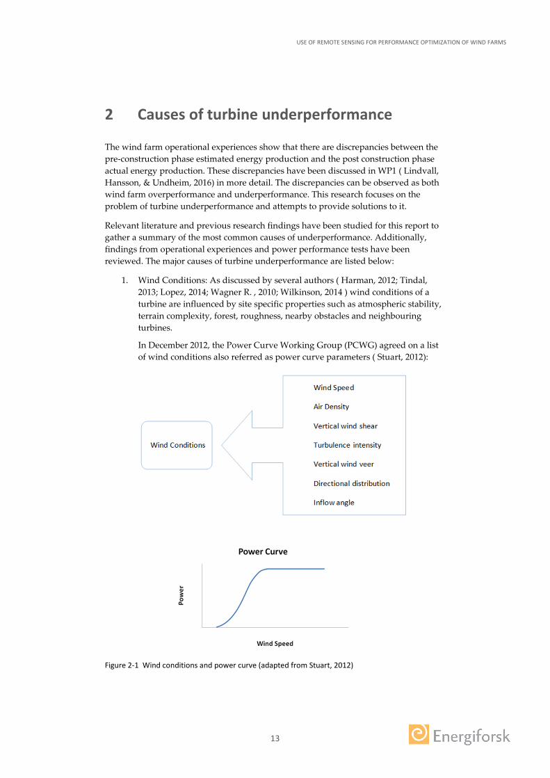
1. Wind Conditions: As discussed by several authors ( Harman, 2012; Tindal, 2013; Lopez, 2014; Wagner R. , 2010; Wilkinson, 2014 ) wind conditions of a turbine are influenced by site specific properties such as atmospheric stability, terrain complexity, forest, roughness, nearby obstacles and neighbouring turbines.
In December 2012, the Power Curve Working Group (PCWG) agreed on a list of wind conditions also referred as power curve parameters ( Stuart, 2012):
Figure 2-1 Wind conditions and power curve (adapted from Stuart, 2012)

USE OF REMOTE SENSING FOR PERFORMANCE OPTIMIZATION OF WIND FARMS
14
a. Wind speed: This is the fundamental power curve parameter to evaluate the wind turbine performance. There are advanced questions to be addressed within the evaluation of wind speeds; such as “How representative is the conventional single wind speed at hub height approach?” and “Is there a need of more detailed wind speed estimation, e.g. rotor-equivalent wind speed as valid for the whole rotor swept area?”
b. Air density: Power production is dependent on the site’s air density. When analysing operational data, there are additional question to be addressed in evaluation of air density such as “Are the conventional methods used to normalize the wind speeds to a reference density accurate for power performance monitoring?” and “Is there a need of more inputs to do more accurate air density estimation of the site?”
In addition to the conventional power curve parameters, PCWG’s list consist of below following parameters to define a more accurate “real world” turbine performance under complex flow conditions.
c. Vertical wind shear.
d. Turbulence intensity.
e. Vertical wind veer.
f. Directional distribution.
g. Inflow angle.
2. Environmental factors: As also pointed out by previously mentioned authors ( Harman, 2012; Tindal, 2013; Lopez, 2014; Wagner R. , 2010; Wilkinson, 2014) environmental factors effecting the aerodynamic properties of wind turbine blades can be listed below:
a. Icing: The icing effects on turbine performance have been discussed in Elforsk Report Part 3 ( Hansson, Lindvall, & Byrkjedal, 2016).
b. Blade degradation: insects, dirt, failure, wear and tear, etc.
3. Wind turbine control:
a. Non optimal controller settings: pre-defined algorithms and parameters such as hysteresis, controller software updates, upgrades ( Tindal, 2013; Lopez, 2014; Wagner R. , 2010; Wilkinson, 2014).
b. Curtailed or de-rated operation: due to loads, grid curtailment, wind sector management, environmental such as noise, shadow, visual, etc. ( Tindal, 2013; Wilkinson, 2014).
c. Component misalignment: yaw, pitch, tilt, etc. ( Tindal, 2013; Wilkinson, 2014).
d. Measurement errors of sensors ( Tindal, 2013; Lopez, 2014; Wagner R. , 2010; Wilkinson, 2014).
4. Maintenance and operations strategies of the wind farm operator.
USE OF REMOTE SENSING FOR PERFORMANCE OPTIMIZATION OF WIND FARMS
15
3 Performance optimization of a wind farm
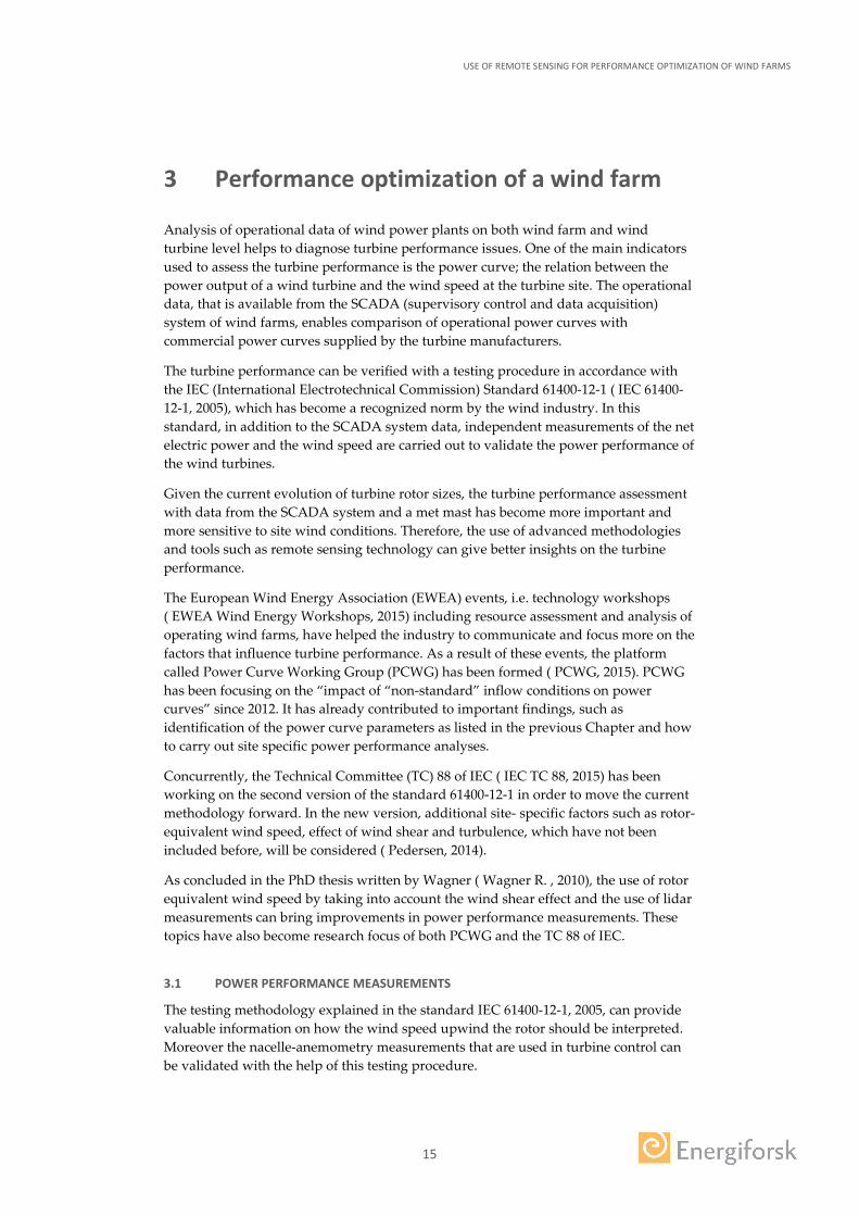
Analysis of operational data of wind power plants on both wind farm and wind turbine level helps to diagnose turbine performance issues. One of the main indicators used to assess the turbine performance is the power curve; the relation between the power output of a wind turbine and the wind speed at the turbine site. The operational data, that is available from the SCADA (supervisory control and data acquisition) system of wind farms, enables comparison of operational power curves with commercial power curves supplied by the turbine manufacturers.
The turbine performance can be verified with a testing procedure in accordance with the IEC (International Electrotechnical Commission) Standard 61400-12-1 ( IEC 61400-12-1, 2005), which has become a recognized norm by the wind industry. In this standard, in addition to the SCADA system data, independent measurements of the net electric power and the wind speed are carried out to validate the power performance of the wind turbines.
Given the current evolution of turbine rotor sizes, the turbine performance assessment with data from the SCADA system and a met mast has become more important and more sensitive to site wind conditions. Therefore, the use of advanced methodologies and tools such as remote sensing technology can give better insights on the turbine performance.
The European Wind Energy Association (EWEA) events, i.e. technology workshops ( EWEA Wind Energy Workshops, 2015) including resource assessment and analysis of operating wind farms, have helped the industry to communicate and focus more on the factors that influence turbine performance. As a result of these events, the platform called Power Curve Working Group (PCWG) has been formed ( PCWG, 2015). PCWG has been focusing on the “impact of “non-standard” inflow conditions on power curves” since 2012. It has already contributed to important findings, such as identification of the power curve parameters as listed in the previous Chapter and how to carry out site specific power performance analyses.
Concurrently, the Technical Committee (TC) 88 of IEC ( IEC TC 88, 2015) has been working on the second version of the standard 61400-12-1 in order to move the current methodology forward. In the new version, additional site- specific factors such as rotor-equivalent wind speed, effect of wind shear and turbulence, which have not been included before, will be considered ( Pedersen, 2014).
As concluded in the PhD thesis written by Wagner ( Wagner R. , 2010), the use of rotor equivalent wind speed by taking into account the wind shear effect and the use of lidar measurements can bring improvements in power performance measurements. These topics have also become research focus of both PCWG and the TC 88 of IEC.
3.1 POWER PERFORMANCE MEASUREMENTS
The testing methodology explained in the standard IEC 61400-12-1, 2005, can provide valuable information on how the wind speed upwind the rotor should be interpreted. Moreover the nacelle-anemometry measurements that are used in turbine control can be validated with the help of this testing procedure.

USE OF REMOTE SENSING FOR PERFORMANCE OPTIMIZATION OF WIND FARMS
16
The IEC standard 61400-12-2 ( IEC 61400-12-2, 2013) focuses on nacelle anemometry and explains how to analyse the nacelle transfer function (NTF) of a turbine. NTF provides the relation between the free wind speeds and the nacelle anemometry based wind speeds. The design phase NTF, predefined in the control system of a turbine, may not be valid for certain site specific conditions. Therefore the assessment of the NTF and then recalibrating it, can improve the performance of the turbines.
It is expected that the new edition of the standard IEC 61400-12-1, 2005 will include ground based remote sensing devices for use in performance testing (in addition to the use of met mast measurements)( Pedersen, 2014). Due to the ability to measure vertical wind profile, the ground based remote sensing has significant advantages especially when the rotor equivalent wind speed is considered in performance evaluation.
The nacelle based remote sensing has not been included within the current development of the standards; however it is already proven to be a good tool ( Wagner, Courtney, Friis Pedersen, Davoust, & Rivera, 2014). As part of future plans on this topic, the International Energy Agency also carries out research, namely Task 32 Lidar (Wind Lidar systems for wind energy deployment) and the subtask 3 namely “lidar procedures for turbine assessment” ( IEA Wind, 2015).
Overall, the power performance methodology can provide:
• Validation of the power curve, therefore correct interpretation of turbine performance.
• Validation of the NTF. • Reduce loads and power production losses.
3.2 OPTIMIZATION MEASURES
In light of topics covered in the Chapter 3 and 3.1, the wind industry focuses on the optimization measures listed below.
1. Improvement of aerodynamic performance of turbine blades:
a. Ice removal and prevention systems: As explained in the previous Chapter, the environmental conditions may change the aerodynamic properties of the wind turbine causing underperformance. De-icing and anti-icing of wind turbine blades in cold climates can improve the aerodynamic performance, and thereby improve the turbine power performance.
b. Maintenance of blades: Cleaning, repairs and renewing the surface of blades reduce the degradation effects on the blades, and thereby improve the turbine performance.
c. Upgrades and specific devices for blade surfaces: Use of vortex generators to enhance performance.
2. Control system optimization:
The control system of a wind turbine can be improved in many ways. Some of the improvements can be facilitated within the existing control system, but there can also be new development areas to be introduced by the help of technological advancements as listed below:

USE OF REMOTE SENSING FOR PERFORMANCE OPTIMIZATION OF WIND FARMS
17
a. Yaw misalignment correction: Yaw misalignment can be diagnosed by measuring the wind direction upwind the rotor relative to the nacelle orientation. Nacelle based remote sensing such as; the nacelle mounted lidar as presented by Wagenaar et al. ( Wagenaar, Davoust, Medawar, Coubard-Millet, & Boorsma, 2014) and the spinner mounted ultrasonic devices as presented by ( Marín & Sundgaard Pedersen, 2014) can be very effective in detecting the yaw misalignment problem. The yaw alignment of a turbine can easily be re-adjusted within the control system. The correction of yaw misalignment and improvement of reaction of yaw system can optimize the performance with increased power production and reduced loads on the turbine.
b. Recalibration of NTF: As discussed in Chapter 3.1 NTF can be recalibrated through power performance measurements.
c. Optimization of the pitch control system: Pitch control system can be optimized through the analysis of SCADA data.
d. Individual pitch control: Wind turbines with individual pitch control system can handle the loads due to wind conditions such as high wind shear better than wind turbines with a conventional pitch control system.
e. Active wake measurements and control: Monitoring and detection of wake interaction of the neighbouring turbines in a wind farm can help to reduce the loads and power production losses. Nacelle based remote sensing devices can be used in wake detection and implemented into the control system.
There are other important aspects to be noted as well within optimization measures as briefly shown:
• The operation and maintenance (O&M) strategies of wind farm operators and wind turbine manufacturers.
• Big data management and analysis procedures. • Communication and transparent knowledge exchange within the wind industry.
3.3 REMOTE SENSING IN PERFORMANCE MONITORING OF WIND FARMS
The use of remote sensing technologies such as sodar and lidar have become good alternatives to the use of conventional met mast or nacelle anemometry in monitoring of performance of wind turbines and wind farms. There are numbers of remote sensing techniques available in field of power performance measurement and testing of onshore wind turbines.
• Ground based vertically profiling with lidars and sodars ( Johansson, Hansson, & Lundén, 2011) ( Clifton & Courtney, 2013) ( Peña, et al., 2015) which are widely used for pre-construction wind resource assessment.
• Ground based scanning: Several commercial lidar examples such as Sgurr Energy’s Galion Lidar, Leosphere’s Wind Cube 3D Lidar, Mitsubishi Electric’s Large-scale Coherent Doppler Lidar System and Lockheed Martin’s Wind Tracer.
• Nacelle based: Nacelle mounted lidars as listed with most common types in Table 3.1, together with spinner mounted ultrasonic anemometer.
USE OF REMOTE SENSING FOR PERFORMANCE OPTIMIZATION OF WIND FARMS
18
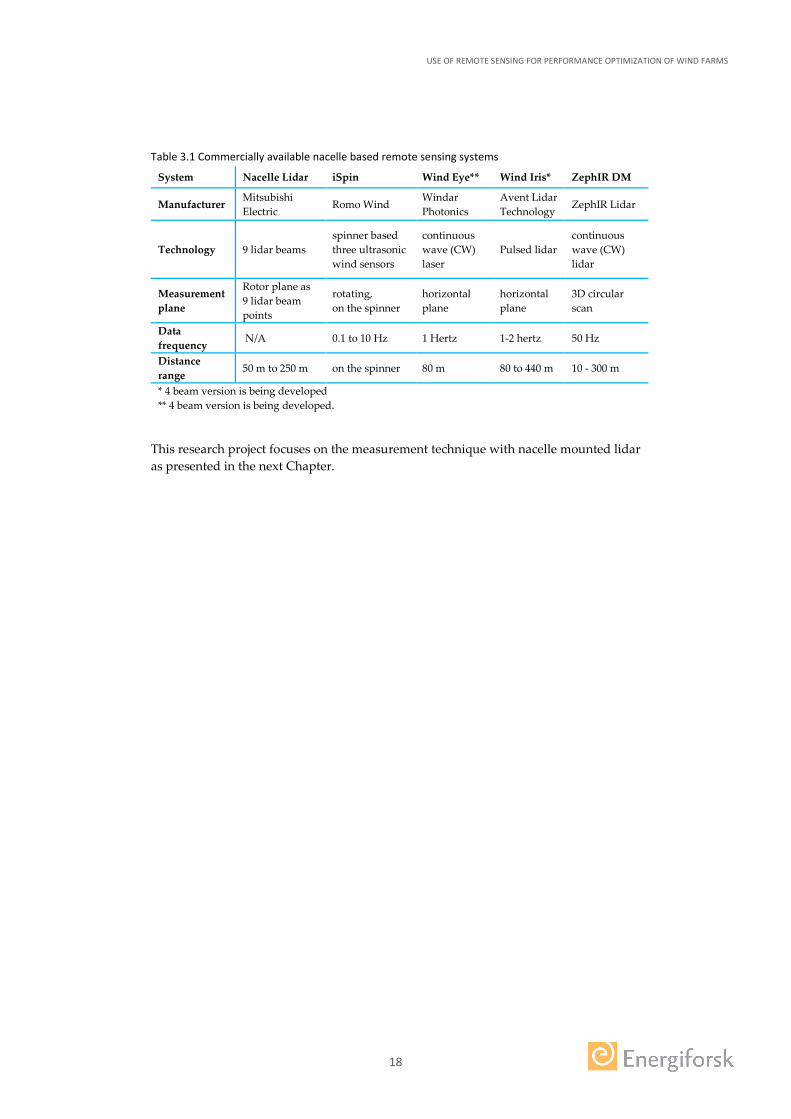
Table 3.1 Commercially available nacelle based remote sensing systems
System Nacelle Lidar iSpin Wind Eye** Wind Iris* ZephIR DM
Manufacturer Mitsubishi Electric
Romo Wind Windar Photonics
Avent Lidar Technology
ZephIR Lidar
Technology 9 lidar beams spinner based three ultrasonic wind sensors
continuous wave (CW) laser
Pulsed lidar continuous wave (CW) lidar
Measurement plane
Rotor plane as 9 lidar beam points
rotating, on the spinner
horizontal plane
horizontal plane
3D circular scan
Data frequency N/A 0.1 to 10 Hz 1 Hertz 1-2 hertz 50 Hz
Distance range 50 m to 250 m on the spinner 80 m 80 to 440 m 10 - 300 m
* 4 beam version is being developed ** 4 beam version is being developed.
This research project focuses on the measurement technique with nacelle mounted lidar as presented in the next Chapter.
USE OF REMOTE SENSING FOR PERFORMANCE OPTIMIZATION OF WIND FARMS
19
4 Nacelle mounted lidar as part of the performance optimization
4.1 DESCRIPTION OF THE MEASUREMENT CAMPAIGNS
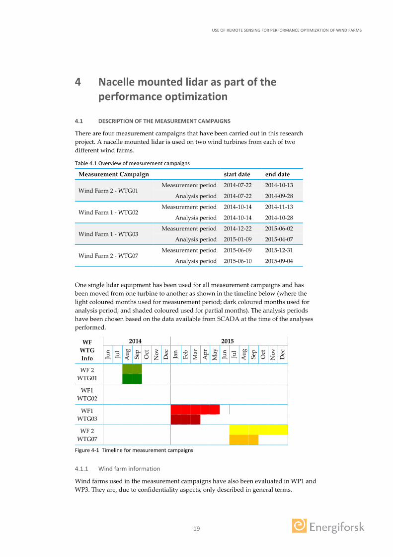
There are four measurement campaigns that have been carried out in this research project. A nacelle mounted lidar is used on two wind turbines from each of two different wind farms.
Table 4.1 Overview of measurement campaigns
Measurement Campaign start date end date
Wind Farm 2 - WTG01 Measurement period 2014-07-22 2014-10-13
Analysis period 2014-07-22 2014-09-28
Wind Farm 1 - WTG02 Measurement period 2014-10-14 2014-11-13
Analysis period 2014-10-14 2014-10-28
Wind Farm 1 - WTG03 Measurement period 2014-12-22 2015-06-02
Analysis period 2015-01-09 2015-04-07
Wind Farm 2 - WTG07 Measurement period 2015-06-09 2015-12-31
Analysis period 2015-06-10 2015-09-04
One single lidar equipment has been used for all measurement campaigns and has been moved from one turbine to another as shown in the timeline below (where the light coloured months used for measurement period; dark coloured months used for analysis period; and shaded coloured used for partial months). The analysis periods have been chosen based on the data available from SCADA at the time of the analyses performed.
WF WTG Info
2014 2015
Jun
Jul
Aug
Se
p O
ct
Nov
D
ec
Jan
Feb
Mar
A
pr
May
Ju
n Ju
l A
ug
Sep
Oct
N
ov
Dec
WF 2 WTG01
WF1 WTG02
WF1 WTG03
WF 2 WTG07
Figure 4-1 Timeline for measurement campaigns
4.1.1 Wind farm information
Wind farms used in the measurement campaigns have also been evaluated in WP1 and WP3. They are, due to confidentiality aspects, only described in general terms.
USE OF REMOTE SENSING FOR PERFORMANCE OPTIMIZATION OF WIND FARMS
20
Wind farm (WF) 1
WF1 is located in a Swedish site with moderately complex terrain and forested land cover experiencing rather long and harsh winters. Average elevation at site is 430 meters above sea level. The minimum distance between neighboring turbines varies from 3.5 to 10.8 rotor diameters with an average of 5.2 rotor diameters. The turbine layout consists of total 17 turbines; five 2.0 MW turbines with hub height 80 m and twelve 2.0 MW turbines with hub height 105 m. The wind farm was built in two stages; five turbines with 80 m hub height have been in operation since 2006 and twelve turbines with 105 m hub height have been in operation since 2008.The wind turbines, which are labelled as WTG 02 and WTG 03, have been tested with nacelle mounted lidar. Both of the turbines have 2.0 MW rated power with a hub height of 80 m.
Wind farm (WF) 2
WF2 is located in southern Sweden, a site with moderately complex terrain and forested land cover, where the winters are in general short and mild. Average elevation at site is 161 meters above sea level. The turbine spacing at the WF2 is changing from 3.9 to 4.7 rotor diameters. WF2 is composed of 11 2.5 MW turbines with a hub height of 98.5 m. It has been operational since 2012. There has been a major upgrade in the operation of WF2 in the beginning of summer 2014. Most of the turbine’s rated power has been adjusted to 2.78 MW with the upgrade.
WTG 01 and WTG 07, which have rated powers of 2.78 MW and 2.53 MW respectively and with same hub height of 98.5 m, have been tested with nacelle mounted lidar.
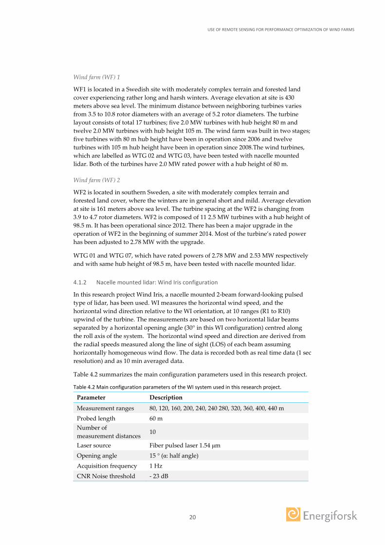
4.1.2 Nacelle mounted lidar: Wind Iris configuration
In this research project Wind Iris, a nacelle mounted 2-beam forward-looking pulsed type of lidar, has been used. WI measures the horizontal wind speed, and the horizontal wind direction relative to the WI orientation, at 10 ranges (R1 to R10) upwind of the turbine. The measurements are based on two horizontal lidar beams separated by a horizontal opening angle (30° in this WI configuration) centred along the roll axis of the system. The horizontal wind speed and direction are derived from the radial speeds measured along the line of sight (LOS) of each beam assuming horizontally homogeneous wind flow. The data is recorded both as real time data (1 sec resolution) and as 10 min averaged data.
Table 4.2 summarizes the main configuration parameters used in this research project.
Table 4.2 Main configuration parameters of the WI system used in this research project.
Parameter Description
Measurement ranges 80, 120, 160, 200, 240, 240 280, 320, 360, 400, 440 m Probed length 60 m Number of measurement distances 10
Laser source Fiber pulsed laser 1.54 μm Opening angle 15 ° (α: half angle) Acquisition frequency 1 Hz CNR Noise threshold - 23 dB
USE OF REMOTE SENSING FOR PERFORMANCE OPTIMIZATION OF WIND FARMS
21
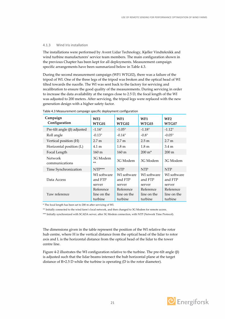
4.1.3 Wind Iris installation
The installations were performed by Avent Lidar Technology, Kjeller Vindteknikk and wind turbine manufacturers’ service team members. The main configuration shown in the previous Chapter has been kept for all deployments. Measurement campaign specific arrangements have been summarized below in Table 4.3.
During the second measurement campaign (WF1 WTG02), there was a failure of the tripod of WI. One of the three legs of the tripod was broken and the optical head of WI tilted towards the nacelle. The WI was sent back to the factory for servicing and recalibration to ensure the good quality of the measurements. During servicing in order to increase the data availability at the ranges close to 2.5 D, the focal length of the WI was adjusted to 200 meters. After servicing, the tripod legs were replaced with the new generation design with a higher safety factor.
Table 4.3 Measurement campaign specific deployment configuration
Campaign Configuration
WF2 WTG01
WF1 WTG02
WF1 WTG03
WF2 WTG07
Pre-tilt angle (β) adjusted -1.14° -1.05° -1.18° -1.12° Roll angle -0.13° -0.14° -0.8° -0.05° Vertical position (H) 2.7 m 2.7 m 2.5 m 2.7 m Horizontal position (L) 4.1 m 1.8 m 1.8 m 3.4 m Focal Length 160 m 160 m 200 m* 200 m
Network communications
3G Modem ** 3G Modem 3G Modem 3G Modem
Time Synchronization NTP*** NTP NTP NTP
Data Access WI software and FTP server
WI software and FTP server
WI software and FTP server
WI software and FTP server
Yaw reference Reference line on the turbine
Reference line on the turbine
Reference line on the turbine
Reference line on the turbine
* The focal length has been set to 200 m after servicing of WI.
** Initially connected to the wind farm’s local network, and then changed to 3G Modem for remote access.
*** Initially synchronized with SCADA server, after 3G Modem connection, with NTP (Network Time Protocol).
The dimensions given in the table represent the position of the WI relative the rotor hub centre, where H is the vertical distance from the optical head of the lidar to rotor axis and L is the horizontal distance from the optical head of the lidar to the tower centre line.
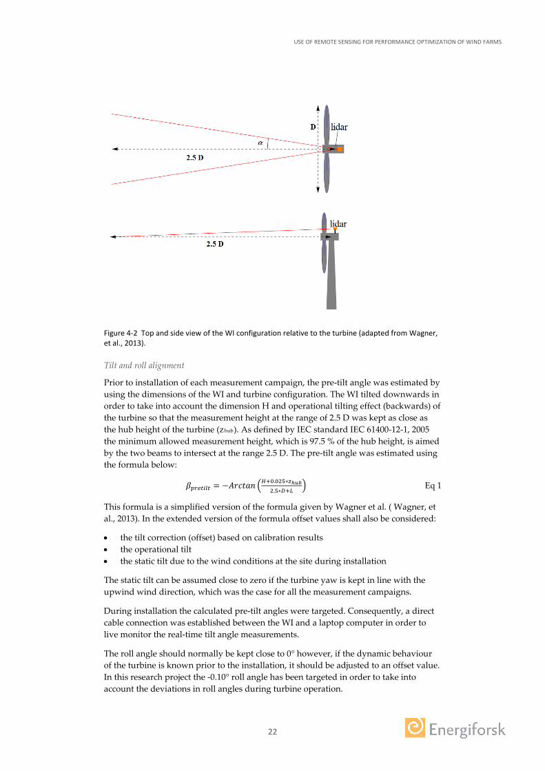
Figure 4-2 illustrates the WI configuration relative to the turbine. The pre-tilt angle (β) is adjusted such that the lidar beams intersect the hub horizontal plane at the target distance of R=2.5 D while the turbine is operating (D is the rotor diameter).
USE OF REMOTE SENSING FOR PERFORMANCE OPTIMIZATION OF WIND FARMS
22
Figure 4-2 Top and side view of the WI configuration relative to the turbine (adapted from Wagner, et al., 2013).
Tilt and roll alignment
Prior to installation of each measurement campaign, the pre-tilt angle was estimated by using the dimensions of the WI and turbine configuration. The WI tilted downwards in order to take into account the dimension H and operational tilting effect (backwards) of the turbine so that the measurement height at the range of 2.5 D was kept as close as the hub height of the turbine (zhub). As defined by IEC standard IEC 61400-12-1, 2005 the minimum allowed measurement height, which is 97.5 % of the hub height, is aimed by the two beams to intersect at the range 2.5 D. The pre-tilt angle was estimated using the formula below:
𝛽𝛽𝑝𝑝𝑝𝑝𝑝𝑝𝑝𝑝𝑝𝑝𝑝𝑝𝑝𝑝 = −𝐴𝐴𝐴𝐴𝐴𝐴𝐴𝐴𝐴𝐴𝐴𝐴 �𝐻𝐻+0.025∗𝑧𝑧ℎ𝑢𝑢𝑢𝑢2.5∗𝐷𝐷+𝐿𝐿
� Eq 1
This formula is a simplified version of the formula given by Wagner et al. ( Wagner, et al., 2013). In the extended version of the formula offset values shall also be considered:
• the tilt correction (offset) based on calibration results • the operational tilt • the static tilt due to the wind conditions at the site during installation
The static tilt can be assumed close to zero if the turbine yaw is kept in line with the upwind wind direction, which was the case for all the measurement campaigns.
During installation the calculated pre-tilt angles were targeted. Consequently, a direct cable connection was established between the WI and a laptop computer in order to live monitor the real-time tilt angle measurements.
The roll angle should normally be kept close to 0° however, if the dynamic behaviour of the turbine is known prior to the installation, it should be adjusted to an offset value. In this research project the -0.10° roll angle has been targeted in order to take into account the deviations in roll angles during turbine operation.
USE OF REMOTE SENSING FOR PERFORMANCE OPTIMIZATION OF WIND FARMS
23
Based on minimum 30 seconds live data, the observed actual tilt and roll angles were kept close to the targeted values. The first two measurement campaigns’ tilt and roll angles have been derived from 1 second real-time data averaged over 30 seconds. For the last two measurement campaigns, WF1 WTG03 and WF2 WTG07, the tilt and roll angles derived from 1 sec data averaged over periods 5 min and 2 min respectively. In order not to disturb the tilt and roll measurements of the WI, none of the installation team members was allowed to be standing on the roof of the turbine nacelle.
Yaw alignment
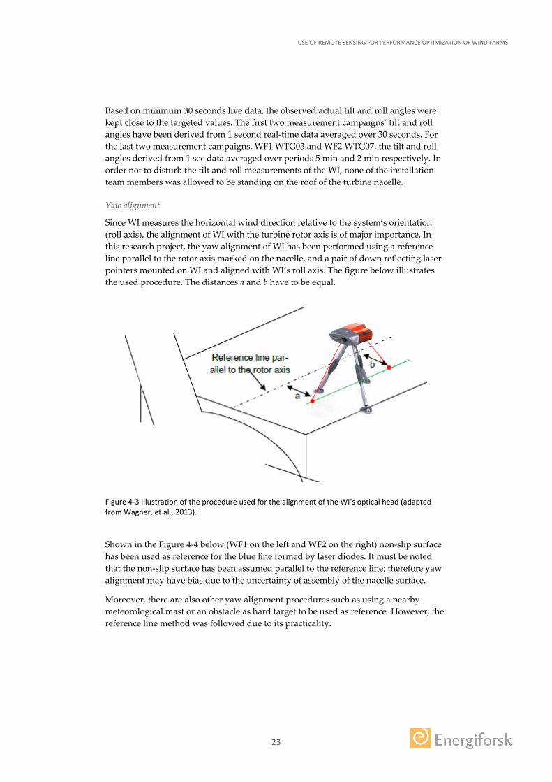
Since WI measures the horizontal wind direction relative to the system’s orientation (roll axis), the alignment of WI with the turbine rotor axis is of major importance. In this research project, the yaw alignment of WI has been performed using a reference line parallel to the rotor axis marked on the nacelle, and a pair of down reflecting laser pointers mounted on WI and aligned with WI’s roll axis. The figure below illustrates the used procedure. The distances a and b have to be equal.
Figure 4-3 Illustration of the procedure used for the alignment of the WI’s optical head (adapted from Wagner, et al., 2013).
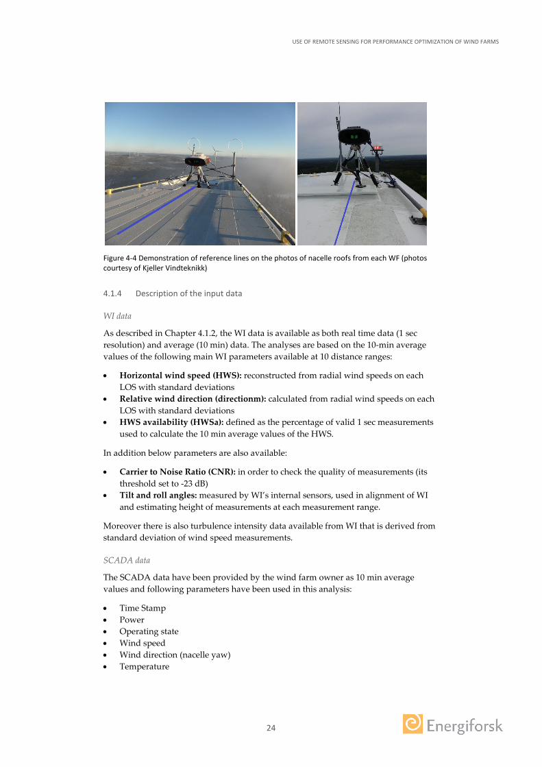
Shown in the Figure 4-4 below (WF1 on the left and WF2 on the right) non-slip surface has been used as reference for the blue line formed by laser diodes. It must be noted that the non-slip surface has been assumed parallel to the reference line; therefore yaw alignment may have bias due to the uncertainty of assembly of the nacelle surface.
Moreover, there are also other yaw alignment procedures such as using a nearby meteorological mast or an obstacle as hard target to be used as reference. However, the reference line method was followed due to its practicality.
USE OF REMOTE SENSING FOR PERFORMANCE OPTIMIZATION OF WIND FARMS
24
Figure 4-4 Demonstration of reference lines on the photos of nacelle roofs from each WF (photos courtesy of Kjeller Vindteknikk)
4.1.4 Description of the input data
WI data
As described in Chapter 4.1.2, the WI data is available as both real time data (1 sec resolution) and average (10 min) data. The analyses are based on the 10-min average values of the following main WI parameters available at 10 distance ranges:
• Horizontal wind speed (HWS): reconstructed from radial wind speeds on each LOS with standard deviations
• Relative wind direction (directionm): calculated from radial wind speeds on each LOS with standard deviations
• HWS availability (HWSa): defined as the percentage of valid 1 sec measurements used to calculate the 10 min average values of the HWS.
In addition below parameters are also available:
• Carrier to Noise Ratio (CNR): in order to check the quality of measurements (its threshold set to -23 dB)
• Tilt and roll angles: measured by WI’s internal sensors, used in alignment of WI and estimating height of measurements at each measurement range.
Moreover there is also turbulence intensity data available from WI that is derived from standard deviation of wind speed measurements.
SCADA data
The SCADA data have been provided by the wind farm owner as 10 min average values and following parameters have been used in this analysis:
• Time Stamp • Power • Operating state • Wind speed • Wind direction (nacelle yaw) • Temperature
USE OF REMOTE SENSING FOR PERFORMANCE OPTIMIZATION OF WIND FARMS
25
WF and WTG data
There are other important input parameters that come from the chosen turbine and its wind farm site.
• Rotor diameter and hub height of the wind turbine • Turbine base elevation • Power curve and its respective air density information to be used as reference in
power curve analysis • Rated, cut-in and cut-out wind speeds and rated power • Long term Weibull parameters (A and k) of the site at the turbine hub height • Digital terrain elevation map in the surrounding of the turbine • Obstacles and neighbour turbines in the surrounding of the turbine (coordinates or
relative position with overall dimensions)
4.1.5 Synchronization of different source data
There are time shifts in the dataset caused by WI logging in UTC and SCADA data logging in local time for all the measurement campaigns. The timestamp of the first measurement campaign (WF2 WTG01) was initially synchronized with SCADA server. After switching to 3G modem connection, synchronization has been established with NTP. The time shifts are 1 hour to 2 hours, depending on local winter and summer time.
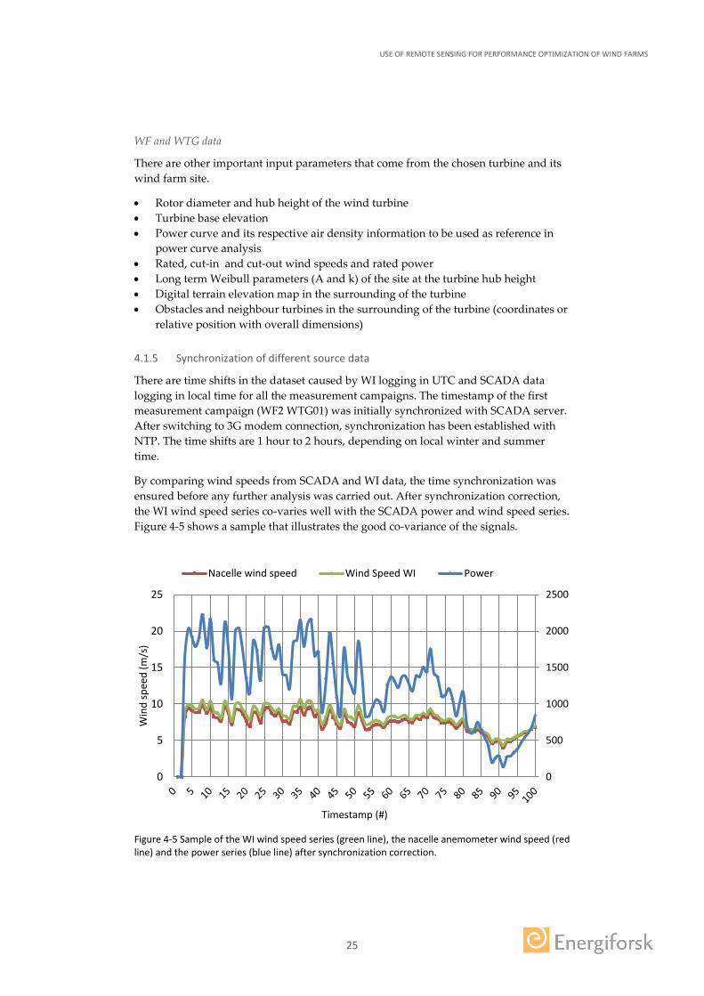
By comparing wind speeds from SCADA and WI data, the time synchronization was ensured before any further analysis was carried out. After synchronization correction, the WI wind speed series co-varies well with the SCADA power and wind speed series. Figure 4-5 shows a sample that illustrates the good co-variance of the signals.
Figure 4-5 Sample of the WI wind speed series (green line), the nacelle anemometer wind speed (red line) and the power series (blue line) after synchronization correction.
0
500
1000
1500
2000
2500
0
5
10
15
20
25
Win
d sp
eed
(m/s
)
Timestamp (#)
Nacelle wind speed Wind Speed WI Power
USE OF REMOTE SENSING FOR PERFORMANCE OPTIMIZATION OF WIND FARMS
26
4.2 YAW ALIGNMENT ANALYSIS
4.2.1 Methodology
Yaw alignment refers to the alignment of the nacelle relative to the direction of the horizontal wind in front of the rotor. Wear; malfunctioning; erroneous or inaccurate alignment of the nacelle’s wind measurement sensors, are possible causes for an inaccurate alignment of the nacelle. In complex terrain, unpredicted effects not accounted for in the nacelle transfer function may also result in yaw misalignment. Significant yaw misalignment leads to underperformance of the wind turbine resulting in production loss and increased loads.
The horizontal wind speed (HWS) given by WI is calculated based on the assumption that the horizontal wind speed at a given distance from the rotor does not vary along the direction parallel to the rotor. It is assumed that both beams see the same horizontal wind speed at each measurement distance. This is the so called, wind homogeneity hypothesis. In order to ensure the validity of this hypothesis, it is necessary to filter out the time periods when one or both of the beams are inside the wake of neighbouring turbines. This and other filters are described in the next Chapters.
4.2.2 Analysis specific filtering
To ensure a reliable analysis of the yaw alignment, the following filters have been applied to the WI 10 min average values:
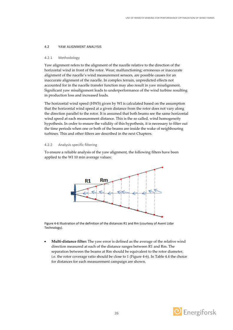
Figure 4-6 Illustration of the definition of the distances R1 and Rm (courtesy of Avent Lidar Technology).
• Multi-distance filter: The yaw error is defined as the average of the relative wind direction measured at each of the distance ranges between R1 and Rm. The separation between the beams at Rm should be equivalent to the rotor diameter, i.e. the rotor coverage ratio should be close to 1 (Figure 4-6). In Table 4.4 the choice for distances for each measurement campaign are shown.
USE OF REMOTE SENSING FOR PERFORMANCE OPTIMIZATION OF WIND FARMS
27
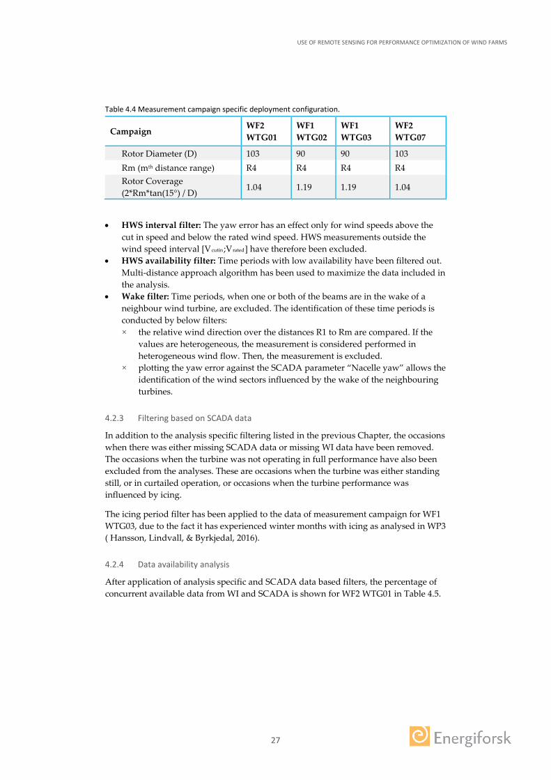
Table 4.4 Measurement campaign specific deployment configuration.
Campaign WF2 WTG01
WF1 WTG02
WF1 WTG03
WF2 WTG07
Rotor Diameter (D) 103 90 90 103 Rm (mth distance range) R4 R4 R4 R4 Rotor Coverage (2*Rm*tan(15°) / D) 1.04 1.19 1.19 1.04
• HWS interval filter: The yaw error has an effect only for wind speeds above the cut in speed and below the rated wind speed. HWS measurements outside the wind speed interval [Vcutin;Vrated] have therefore been excluded.
• HWS availability filter: Time periods with low availability have been filtered out. Multi-distance approach algorithm has been used to maximize the data included in the analysis.
• Wake filter: Time periods, when one or both of the beams are in the wake of a neighbour wind turbine, are excluded. The identification of these time periods is conducted by below filters: × the relative wind direction over the distances R1 to Rm are compared. If the
values are heterogeneous, the measurement is considered performed in heterogeneous wind flow. Then, the measurement is excluded.
× plotting the yaw error against the SCADA parameter “Nacelle yaw” allows the identification of the wind sectors influenced by the wake of the neighbouring turbines.
4.2.3 Filtering based on SCADA data
In addition to the analysis specific filtering listed in the previous Chapter, the occasions when there was either missing SCADA data or missing WI data have been removed. The occasions when the turbine was not operating in full performance have also been excluded from the analyses. These are occasions when the turbine was either standing still, or in curtailed operation, or occasions when the turbine performance was influenced by icing.
The icing period filter has been applied to the data of measurement campaign for WF1 WTG03, due to the fact it has experienced winter months with icing as analysed in WP3 ( Hansson, Lindvall, & Byrkjedal, 2016).
4.2.4 Data availability analysis
After application of analysis specific and SCADA data based filters, the percentage of concurrent available data from WI and SCADA is shown for WF2 WTG01 in Table 4.5.
USE OF REMOTE SENSING FOR PERFORMANCE OPTIMIZATION OF WIND FARMS
28
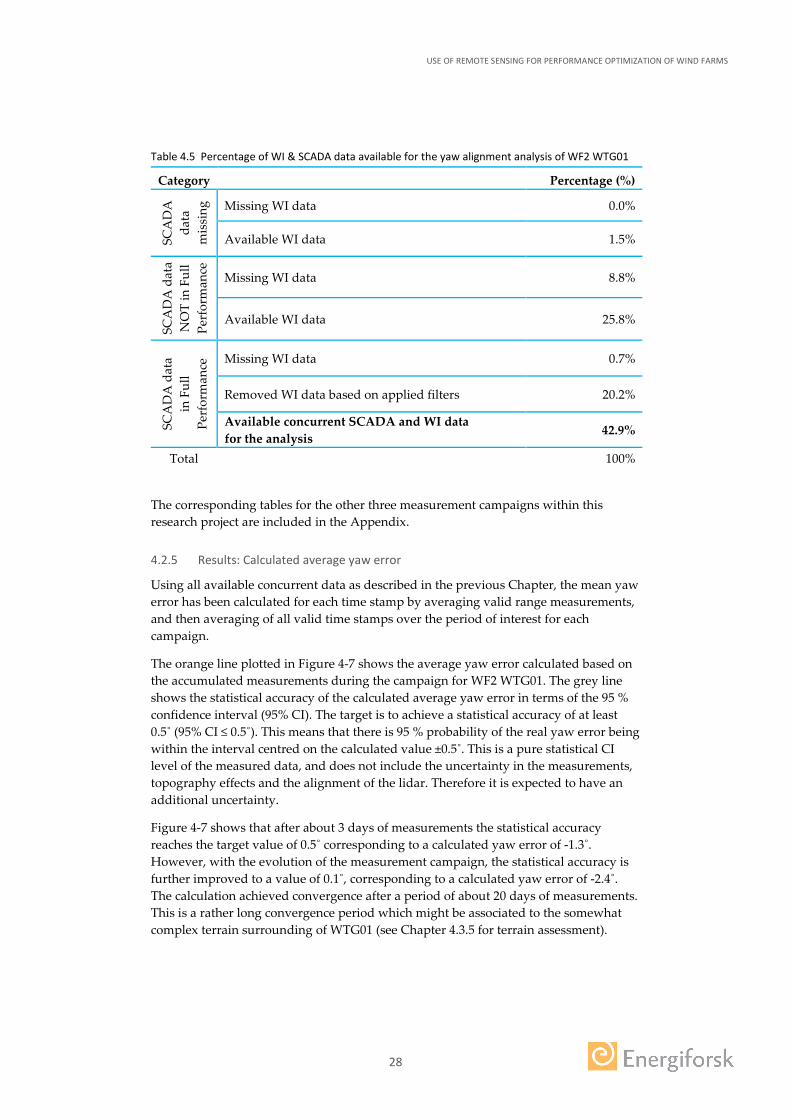
Table 4.5 Percentage of WI & SCADA data available for the yaw alignment analysis of WF2 WTG01
Category Percentage (%) SC
AD
A
data
m
issi
ng
Missing WI data 0.0%
Available WI data 1.5%
SCA
DA
dat
a N
OT
in F
ull
Perf
orm
ance
Missing WI data 8.8%
Available WI data 25.8%
SCA
DA
dat
a
in F
ull
Perf
orm
ance
Missing WI data 0.7%
Removed WI data based on applied filters 20.2%
Available concurrent SCADA and WI data for the analysis 42.9%
Total 100%
The corresponding tables for the other three measurement campaigns within this research project are included in the Appendix.
4.2.5 Results: Calculated average yaw error
Using all available concurrent data as described in the previous Chapter, the mean yaw error has been calculated for each time stamp by averaging valid range measurements, and then averaging of all valid time stamps over the period of interest for each campaign.
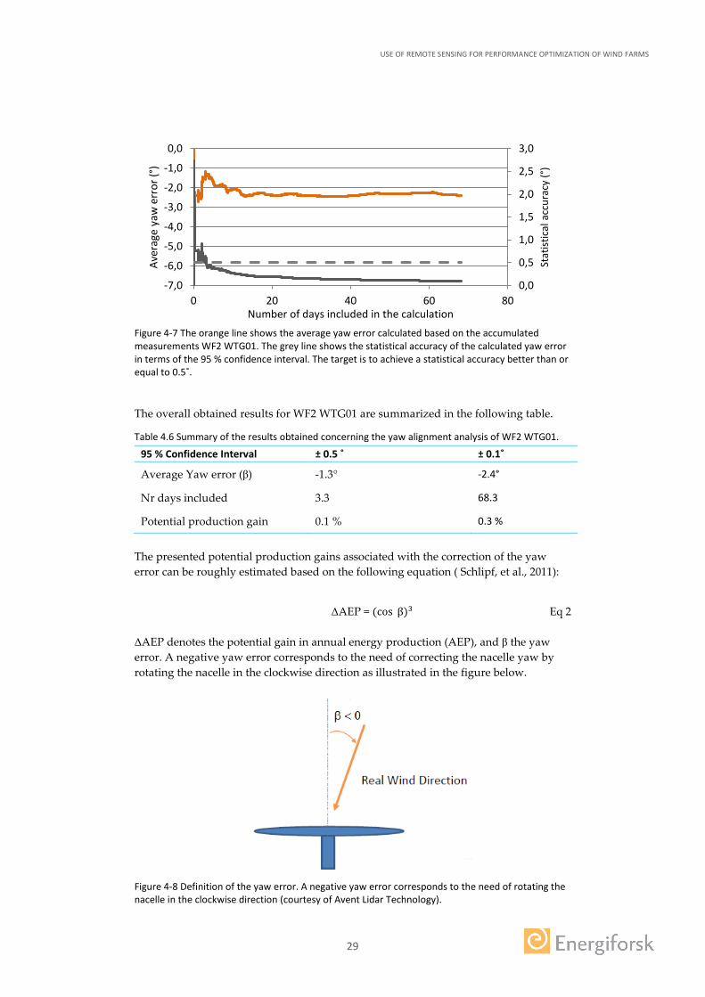
The orange line plotted in Figure 4-7 shows the average yaw error calculated based on the accumulated measurements during the campaign for WF2 WTG01. The grey line shows the statistical accuracy of the calculated average yaw error in terms of the 95 % confidence interval (95% CI). The target is to achieve a statistical accuracy of at least 0.5˚ (95% CI ≤ 0.5˚). This means that there is 95 % probability of the real yaw error being within the interval centred on the calculated value ±0.5˚. This is a pure statistical CI level of the measured data, and does not include the uncertainty in the measurements, topography effects and the alignment of the lidar. Therefore it is expected to have an additional uncertainty.
Figure 4-7 shows that after about 3 days of measurements the statistical accuracy reaches the target value of 0.5˚ corresponding to a calculated yaw error of -1.3˚. However, with the evolution of the measurement campaign, the statistical accuracy is further improved to a value of 0.1˚, corresponding to a calculated yaw error of -2.4˚. The calculation achieved convergence after a period of about 20 days of measurements. This is a rather long convergence period which might be associated to the somewhat complex terrain surrounding of WTG01 (see Chapter 4.3.5 for terrain assessment).
USE OF REMOTE SENSING FOR PERFORMANCE OPTIMIZATION OF WIND FARMS
29
Figure 4-7 The orange line shows the average yaw error calculated based on the accumulated measurements WF2 WTG01. The grey line shows the statistical accuracy of the calculated yaw error in terms of the 95 % confidence interval. The target is to achieve a statistical accuracy better than or equal to 0.5˚.
The overall obtained results for WF2 WTG01 are summarized in the following table.
Table 4.6 Summary of the results obtained concerning the yaw alignment analysis of WF2 WTG01.
95 % Confidence Interval ± 0.5 ˚ ± 0.1˚
Average Yaw error (β) -1.3° -2.4°
Nr days included 3.3 68.3
Potential production gain 0.1 % 0.3 %
The presented potential production gains associated with the correction of the yaw error can be roughly estimated based on the following equation ( Schlipf, et al., 2011):
ΔAEP = (cos β)3 Eq 2
ΔAEP denotes the potential gain in annual energy production (AEP), and β the yaw error. A negative yaw error corresponds to the need of correcting the nacelle yaw by rotating the nacelle in the clockwise direction as illustrated in the figure below.
Figure 4-8 Definition of the yaw error. A negative yaw error corresponds to the need of rotating the nacelle in the clockwise direction (courtesy of Avent Lidar Technology).
0,0
0,5
1,0
1,5
2,0
2,5
3,0
-7,0
-6,0
-5,0
-4,0
-3,0
-2,0
-1,0
0,0
0 20 40 60 80
Stat
istic
al a
ccur
acy
(°)
Aver
age
yaw
err
or (°
)
Number of days included in the calculation
USE OF REMOTE SENSING FOR PERFORMANCE OPTIMIZATION OF WIND FARMS
30
The results (tables and figures) for the other three measurement campaigns within this research project are included in the Appendix.
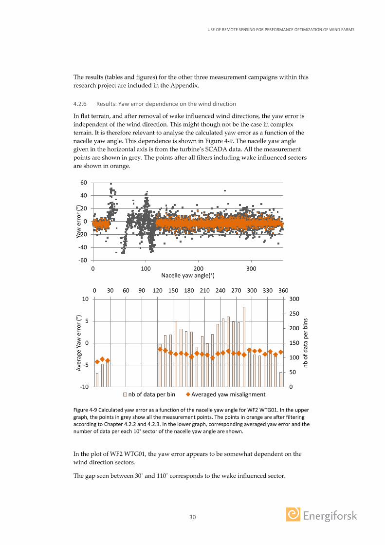
4.2.6 Results: Yaw error dependence on the wind direction
In flat terrain, and after removal of wake influenced wind directions, the yaw error is independent of the wind direction. This might though not be the case in complex terrain. It is therefore relevant to analyse the calculated yaw error as a function of the nacelle yaw angle. This dependence is shown in Figure 4-9. The nacelle yaw angle given in the horizontal axis is from the turbine’s SCADA data. All the measurement points are shown in grey. The points after all filters including wake influenced sectors are shown in orange.
Figure 4-9 Calculated yaw error as a function of the nacelle yaw angle for WF2 WTG01. In the upper graph, the points in grey show all the measurement points. The points in orange are after filtering according to Chapter 4.2.2 and 4.2.3. In the lower graph, corresponding averaged yaw error and the number of data per each 10° sector of the nacelle yaw angle are shown.
In the plot of WF2 WTG01, the yaw error appears to be somewhat dependent on the wind direction sectors.
The gap seen between 30˚ and 110˚ corresponds to the wake influenced sector.
-60
-40
-20
0
20
40
60
0 100 200 300
Yaw
err
or (°
)
Nacelle yaw angle(°)
0
50
100
150
200
250
300
-10
-5
0
5
100 30 60 90 120 150 180 210 240 270 300 330 360
nb o
f dat
a pe
r bin
s
Aver
age
Yaw
err
or (°
)
nb of data per bin Averaged yaw misalignment
USE OF REMOTE SENSING FOR PERFORMANCE OPTIMIZATION OF WIND FARMS
31
It must be noted that the scatter of yaw error shows that instantaneous 10 minute mean yaw error is changing between -10° to +10°. Therefore, even though the overall average yaw error is negligible, it is recommended to investigate potential energy production improvements within the yaw system by keeping the turbine better aligned with upwind flow.
The corresponding plots for the other three measurement campaigns within this research project are included in the Appendix.
4.3 NACELLE ANEMOMETER CALIBRATION ANALYSIS
Conventional wind turbines have nacelle mounted anemometers to measure the wind speed the rotor is experiencing. However the nacelle anemometers are located behind the rotor and are therefore exposed to the wake effects of the rotor and the flow disturbance caused by the nacelle. In order to correct for these effects, as discussed in Chapter 3.1, a NTF is applied to the measured wind speeds by the control system. Correcting for the wake effects is however a complicated task which is reflected on the accuracy of the NTF. Having a nacelle mounted lidar system that measures the wind conditions upwind the rotor gives the possibility of analyzing the nacelle transfer function. The results from this analysis are presented in the following Chapters.
The selected wind data have been normalized to the ISO standard atmosphere reference air density (sea level air density of 1.225 kg/m3). The normalized wind speeds for each bin have been estimated by the equation given by the IEC standard IEC 61400-12-1, 2005:
𝑉𝑉𝑛𝑛 = 𝑉𝑉10𝑚𝑚𝑝𝑝𝑛𝑛 ∗ �𝜌𝜌10𝑚𝑚𝑚𝑚𝑚𝑚𝜌𝜌0
�13
P
Eq 3
where Vn is the normalized wind speed; V10 is the measured wind speed averaged over 10 min; ρ0 is the reference air density and ρ10min is the derived 10 min averaged air density. The derived air density is calculated by using 10 min temperature data available in the SCADA data and the derived 10 min pressure using the turbine’s hub altitude above sea level.
4.3.1 Analysis specific filtering
The following filters have been applied to the WI 10 min average values:
One-distance filter: As described in Chapter 4.1.3, Wind Iris has been pre-tilted such that the line of sight of the each beam crosses the hub height plane at a distance of about 2.5 D. The IEC standard IEC 61400-12-1, 2005 requirement for measurement distance is defined for a met mast which is between 2 and the 4 times the rotor diameter, with 2.5 D being recommended distance. Due to use of the default of the range configuration of Wind Iris, in this research project the measurement distance is chosen from the ranges that are close to 2.5 D as shown in Table 4.7 for each measurement campaign. The chosen measurement distance is hereafter denoted as the reference distance.
USE OF REMOTE SENSING FOR PERFORMANCE OPTIMIZATION OF WIND FARMS
32
Table 4.7 Measurement campaign specific deployment configuration.
Campaign WF2 WTG01
WF1 WTG02
WF1 WTG03
WF2 WTG07
Rotor Diameter (D) 103 90 90 103 Reference Distance R5 R5 R4 R5 Reference Distance as # of D 2.3 D 2.7 D 2.2 D 2.3 D
• RWS availability filter: The availability of the measurements used to calculate the 10-min average radial wind speed (RWS) for each line of sight (RWS_beam1 and RWS_beam2) has to be larger than 80 % for the chosen distance. This filter is more restrictive than the HWS availability filter applied in the yaw alignment analysis, insuring the robustness required for NTF analysis.
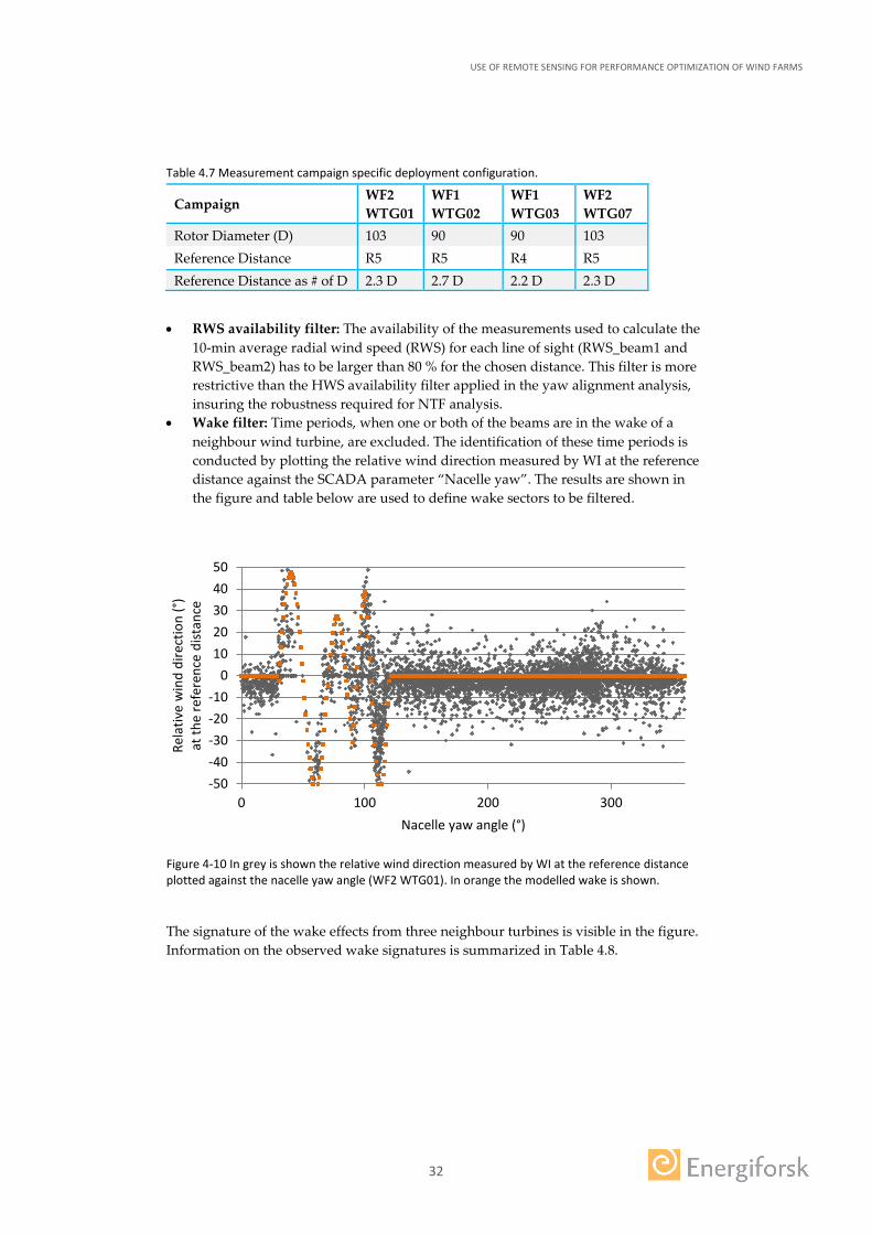
• Wake filter: Time periods, when one or both of the beams are in the wake of a neighbour wind turbine, are excluded. The identification of these time periods is conducted by plotting the relative wind direction measured by WI at the reference distance against the SCADA parameter “Nacelle yaw”. The results are shown in the figure and table below are used to define wake sectors to be filtered.
Figure 4-10 In grey is shown the relative wind direction measured by WI at the reference distance plotted against the nacelle yaw angle (WF2 WTG01). In orange the modelled wake is shown.
The signature of the wake effects from three neighbour turbines is visible in the figure. Information on the observed wake signatures is summarized in Table 4.8.
-50-40-30-20-10
01020304050
0 100 200 300
Rela
tive
win
d di
rect
ion
(°)
at th
e re
fere
nce
dist
ance
Nacelle yaw angle (°)
USE OF REMOTE SENSING FOR PERFORMANCE OPTIMIZATION OF WIND FARMS
33
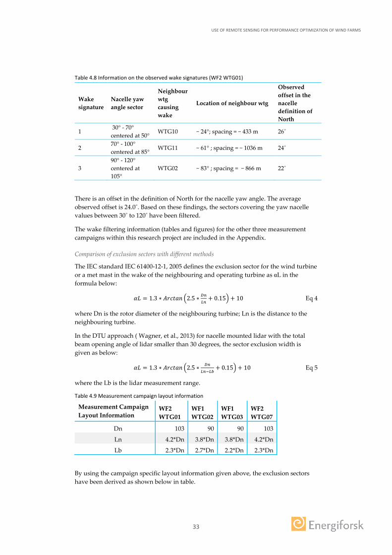
Table 4.8 Information on the observed wake signatures (WF2 WTG01)
Wake signature
Nacelle yaw angle sector
Neighbour wtg causing wake
Location of neighbour wtg
Observed offset in the nacelle definition of North
1 30° - 70° centered at 50°
WTG10 ~ 24°; spacing = ~ 433 m 26˚
2 70° - 100° centered at 85° WTG11 ~ 61° ; spacing = ~ 1036 m 24˚
3 90° - 120° centered at 105°
WTG02 ~ 83° ; spacing = ~ 866 m 22˚
There is an offset in the definition of North for the nacelle yaw angle. The average observed offset is 24.0˚. Based on these findings, the sectors covering the yaw nacelle values between 30˚ to 120˚ have been filtered.
The wake filtering information (tables and figures) for the other three measurement campaigns within this research project are included in the Appendix.
Comparison of exclusion sectors with different methods
The IEC standard IEC 61400-12-1, 2005 defines the exclusion sector for the wind turbine or a met mast in the wake of the neighbouring and operating turbine as αL in the formula below:
𝛼𝛼𝛼𝛼 = 1.3 ∗ 𝐴𝐴𝐴𝐴𝐴𝐴𝐴𝐴𝐴𝐴𝐴𝐴 �2.5 ∗ 𝐷𝐷𝑛𝑛𝐿𝐿𝑛𝑛
+ 0.15� + 10 Eq 4
where Dn is the rotor diameter of the neighbouring turbine; Ln is the distance to the neighbouring turbine.
In the DTU approach ( Wagner, et al., 2013) for nacelle mounted lidar with the total beam opening angle of lidar smaller than 30 degrees, the sector exclusion width is given as below:
𝛼𝛼𝛼𝛼 = 1.3 ∗ 𝐴𝐴𝐴𝐴𝐴𝐴𝐴𝐴𝐴𝐴𝐴𝐴 �2.5 ∗ 𝐷𝐷𝑛𝑛𝐿𝐿𝑛𝑛−𝐿𝐿𝐿𝐿
+ 0.15� + 10 Eq 5
where the Lb is the lidar measurement range.
Table 4.9 Measurement campaign layout information
Measurement Campaign Layout Information
WF2 WTG01
WF1 WTG02
WF1 WTG03
WF2 WTG07
Dn 103 90 90 103
Ln 4.2*Dn 3.8*Dn 3.8*Dn 4.2*Dn
Lb 2.3*Dn 2.7*Dn 2.2*Dn 2.3*Dn
By using the campaign specific layout information given above, the exclusion sectors have been derived as shown below in table.
USE OF REMOTE SENSING FOR PERFORMANCE OPTIMIZATION OF WIND FARMS
34
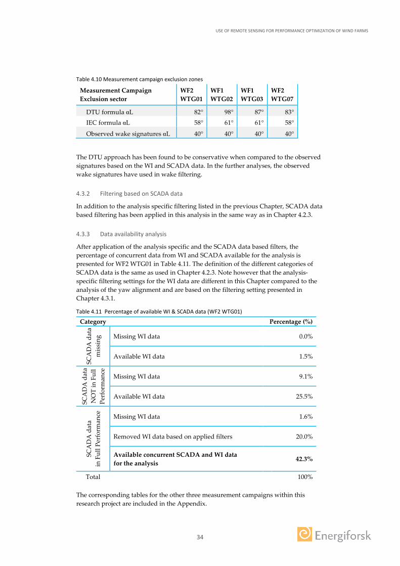
Table 4.10 Measurement campaign exclusion zones
Measurement Campaign Exclusion sector
WF2 WTG01
WF1 WTG02
WF1 WTG03
WF2 WTG07
DTU formula αL 82° 98° 87° 83° IEC formula αL 58° 61° 61° 58°
Observed wake signatures αL 40° 40° 40° 40°
The DTU approach has been found to be conservative when compared to the observed signatures based on the WI and SCADA data. In the further analyses, the observed wake signatures have used in wake filtering.
4.3.2 Filtering based on SCADA data
In addition to the analysis specific filtering listed in the previous Chapter, SCADA data based filtering has been applied in this analysis in the same way as in Chapter 4.2.3.
4.3.3 Data availability analysis
After application of the analysis specific and the SCADA data based filters, the percentage of concurrent data from WI and SCADA available for the analysis is presented for WF2 WTG01 in Table 4.11. The definition of the different categories of SCADA data is the same as used in Chapter 4.2.3. Note however that the analysis-specific filtering settings for the WI data are different in this Chapter compared to the analysis of the yaw alignment and are based on the filtering setting presented in Chapter 4.3.1.
Table 4.11 Percentage of available WI & SCADA data (WF2 WTG01)
Category Percentage (%)
SCA
DA
dat
a m
issi
ng Missing WI data 0.0%
Available WI data 1.5%
SCA
DA
dat
a N
OT
in F
ull
Perf
orm
ance
Missing WI data 9.1%
Available WI data 25.5%
SCA
DA
dat
a
in F
ull P
erfo
rman
ce
Missing WI data 1.6%
Removed WI data based on applied filters 20.0%
Available concurrent SCADA and WI data for the analysis
42.3%
Total 100% The corresponding tables for the other three measurement campaigns within this research project are included in the Appendix.
USE OF REMOTE SENSING FOR PERFORMANCE OPTIMIZATION OF WIND FARMS
35
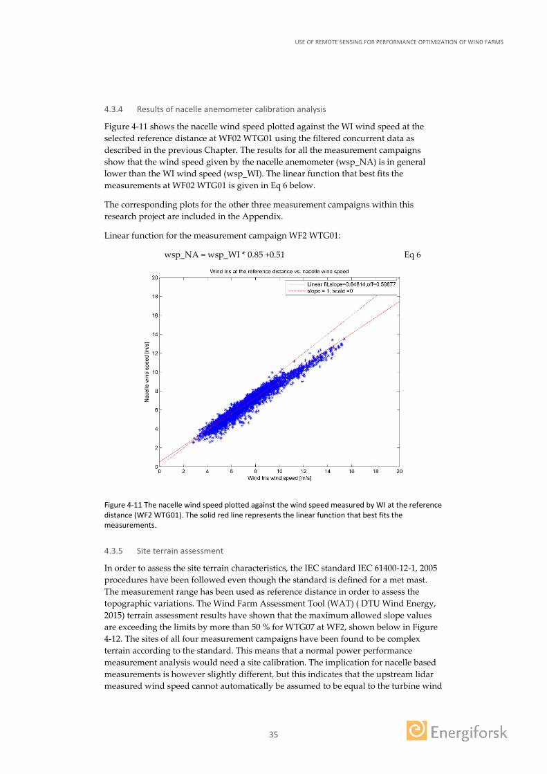
4.3.4 Results of nacelle anemometer calibration analysis
Figure 4-11 shows the nacelle wind speed plotted against the WI wind speed at the selected reference distance at WF02 WTG01 using the filtered concurrent data as described in the previous Chapter. The results for all the measurement campaigns show that the wind speed given by the nacelle anemometer (wsp_NA) is in general lower than the WI wind speed (wsp_WI). The linear function that best fits the measurements at WF02 WTG01 is given in Eq 6 below.
The corresponding plots for the other three measurement campaigns within this research project are included in the Appendix.
Linear function for the measurement campaign WF2 WTG01:
wsp_NA = wsp_WI * 0.85 +0.51 Eq 6
Figure 4-11 The nacelle wind speed plotted against the wind speed measured by WI at the reference distance (WF2 WTG01). The solid red line represents the linear function that best fits the measurements.
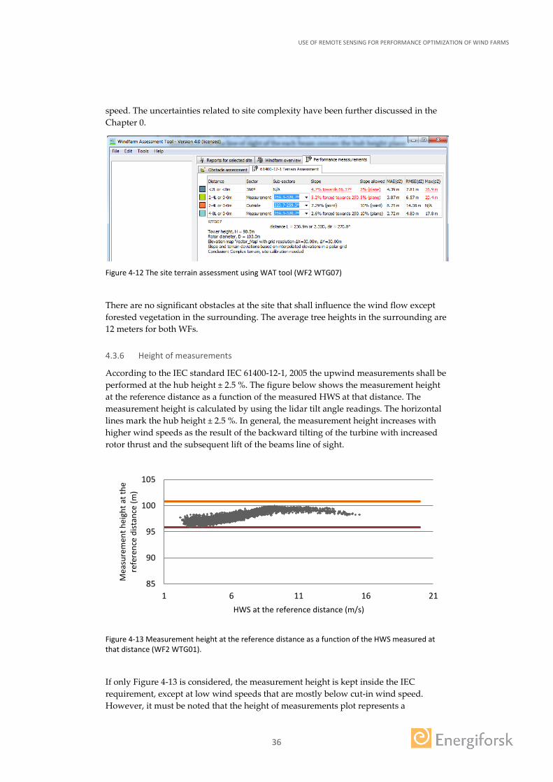
4.3.5 Site terrain assessment
In order to assess the site terrain characteristics, the IEC standard IEC 61400-12-1, 2005 procedures have been followed even though the standard is defined for a met mast. The measurement range has been used as reference distance in order to assess the topographic variations. The Wind Farm Assessment Tool (WAT) ( DTU Wind Energy, 2015) terrain assessment results have shown that the maximum allowed slope values are exceeding the limits by more than 50 % for WTG07 at WF2, shown below in Figure 4-12. The sites of all four measurement campaigns have been found to be complex terrain according to the standard. This means that a normal power performance measurement analysis would need a site calibration. The implication for nacelle based measurements is however slightly different, but this indicates that the upstream lidar measured wind speed cannot automatically be assumed to be equal to the turbine wind
USE OF REMOTE SENSING FOR PERFORMANCE OPTIMIZATION OF WIND FARMS
36
speed. The uncertainties related to site complexity have been further discussed in the Chapter 0.
Figure 4-12 The site terrain assessment using WAT tool (WF2 WTG07)
There are no significant obstacles at the site that shall influence the wind flow except forested vegetation in the surrounding. The average tree heights in the surrounding are 12 meters for both WFs.
4.3.6 Height of measurements
According to the IEC standard IEC 61400-12-1, 2005 the upwind measurements shall be performed at the hub height ± 2.5 %. The figure below shows the measurement height at the reference distance as a function of the measured HWS at that distance. The measurement height is calculated by using the lidar tilt angle readings. The horizontal lines mark the hub height ± 2.5 %. In general, the measurement height increases with higher wind speeds as the result of the backward tilting of the turbine with increased rotor thrust and the subsequent lift of the beams line of sight.
Figure 4-13 Measurement height at the reference distance as a function of the HWS measured at that distance (WF2 WTG01).
If only Figure 4-13 is considered, the measurement height is kept inside the IEC requirement, except at low wind speeds that are mostly below cut-in wind speed. However, it must be noted that the height of measurements plot represents a
85
90
95
100
105
1 6 11 16 21
Mea
sure
men
t hei
ght a
t the
re
fere
nce
dist
ance
(m)
HWS at the reference distance (m/s)
USE OF REMOTE SENSING FOR PERFORMANCE OPTIMIZATION OF WIND FARMS
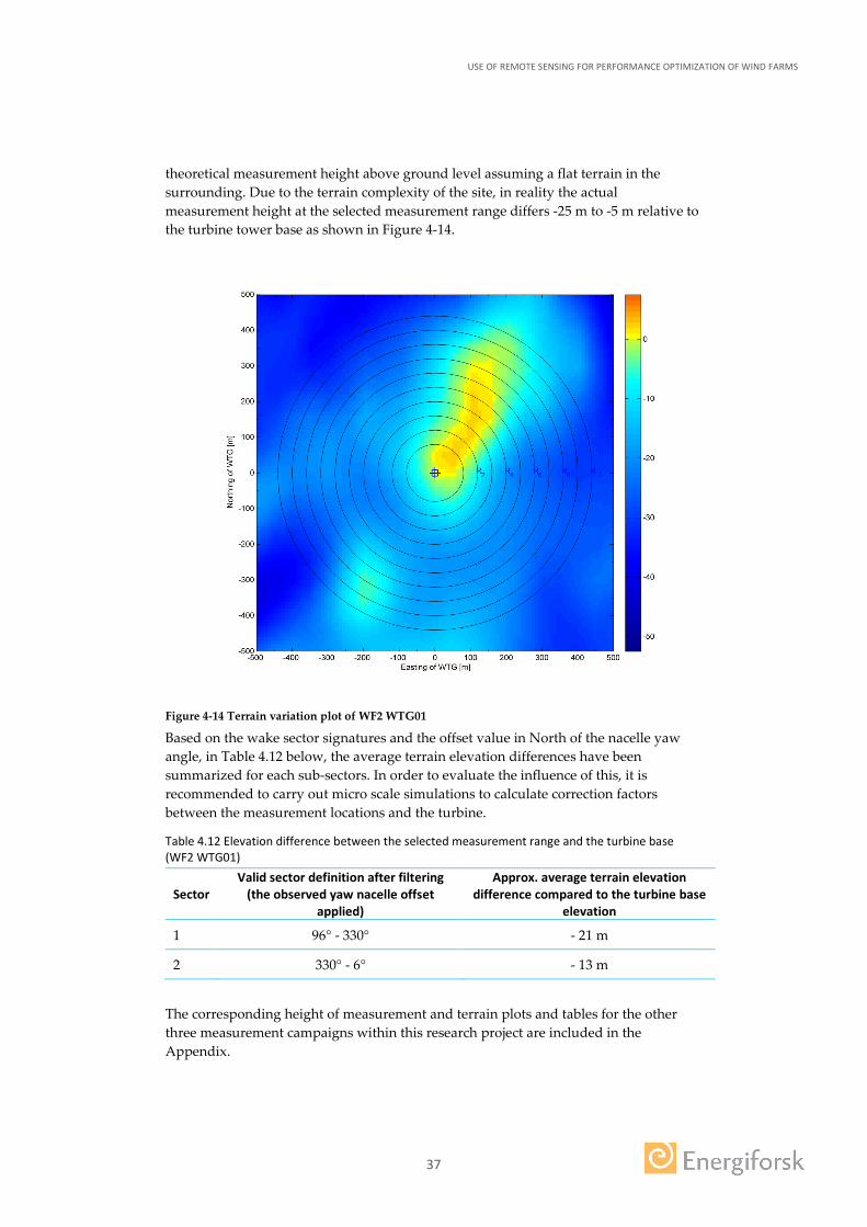
37
theoretical measurement height above ground level assuming a flat terrain in the surrounding. Due to the terrain complexity of the site, in reality the actual measurement height at the selected measurement range differs -25 m to -5 m relative to the turbine tower base as shown in Figure 4-14.
Figure 4-14 Terrain variation plot of WF2 WTG01
Based on the wake sector signatures and the offset value in North of the nacelle yaw angle, in Table 4.12 below, the average terrain elevation differences have been summarized for each sub-sectors. In order to evaluate the influence of this, it is recommended to carry out micro scale simulations to calculate correction factors between the measurement locations and the turbine.
Table 4.12 Elevation difference between the selected measurement range and the turbine base (WF2 WTG01)
Sector Valid sector definition after filtering
(the observed yaw nacelle offset applied)
Approx. average terrain elevation difference compared to the turbine base
elevation
1 96° - 330° - 21 m
2 330° - 6° - 13 m
The corresponding height of measurement and terrain plots and tables for the other three measurement campaigns within this research project are included in the Appendix.
USE OF REMOTE SENSING FOR PERFORMANCE OPTIMIZATION OF WIND FARMS
38
4.4 POWER CURVE ANALYSIS
4.4.1 Methodology
The power curve analysis, as being part of turbine performance analysis, is regulated by IEC standard IEC 61400-12-1, 2005. This standard addresses to the case where a met mast is used. The use of a nacelle based lidar system has not yet been regulated by an IEC standard. However, DTU (Technical University of Denmark) Wind Energy Department has developed a procedure for the use of a nacelle mounted lidar (2-beam, forward looking) for power performance measurement, analysis and reporting ( Wagner, et al., 2013). Both IEC and DTU procedures have been used as basis to power curve analysis of the measurement campaigns within the current research project.
The filtering of the input data used in this analysis is the same as used for the analysis of the NTF described in Chapter 4.3.1 and 4.3.2.
In order to take into account the dependence of the produced power on the air density, the WI and the nacelle anemometer wind speeds have been normalized to the reference air density according to the procedure defined in the IEC standard IEC 61400-12-1, 2005. The normalization procedure explained in Chapter 4.3.
The wind speed data is sorted into 0.5 m/s wide bins. A minimum of 3 data points is required within each bin.
4.4.2 Results: measured power curve
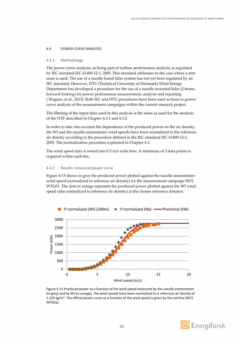
Figure 4-15 shows in grey the produced power plotted against the nacelle anemometer wind speed (normalized to reference air density) for the measurement campaign WF2 WTG01. The dots in orange represent the produced power plotted against the WI wind speed (also normalized to reference air density) at the chosen reference distance.
Figure 4-15 Produced power as a function of the wind speed measured by the nacelle anemometer (in grey) and by WI (in orange). The wind speeds have been normalized to a reference air density of 1.225 kg/m3. The official power curve as a function of the wind speed is given by the red line (WF2 WTG01).
0
500
1000
1500
2000
2500
3000
0 5 10 15 20
Pow
er (k
W)
Wind speed (m/s)
P normalized (WI) (240m) P normalized (Na) Pnominal (kW)
USE OF REMOTE SENSING FOR PERFORMANCE OPTIMIZATION OF WIND FARMS
39
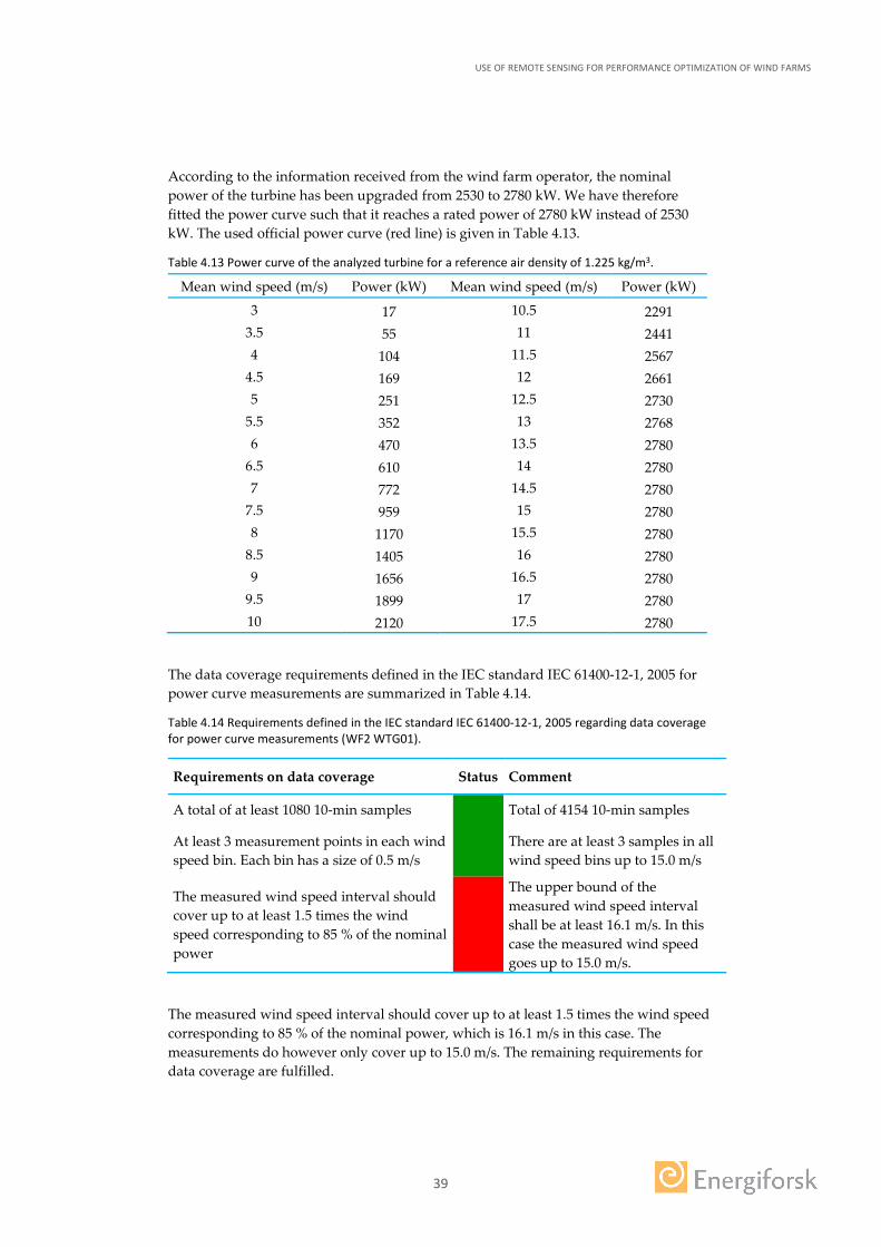
According to the information received from the wind farm operator, the nominal power of the turbine has been upgraded from 2530 to 2780 kW. We have therefore fitted the power curve such that it reaches a rated power of 2780 kW instead of 2530 kW. The used official power curve (red line) is given in Table 4.13.
Table 4.13 Power curve of the analyzed turbine for a reference air density of 1.225 kg/m3.
Mean wind speed (m/s) Power (kW) Mean wind speed (m/s) Power (kW)
3 17 10.5 2291 3.5 55 11 2441 4 104 11.5 2567
4.5 169 12 2661 5 251 12.5 2730
5.5 352 13 2768 6 470 13.5 2780
6.5 610 14 2780 7 772 14.5 2780
7.5 959 15 2780 8 1170 15.5 2780
8.5 1405 16 2780 9 1656 16.5 2780
9.5 1899 17 2780 10 2120 17.5 2780
The data coverage requirements defined in the IEC standard IEC 61400-12-1, 2005 for power curve measurements are summarized in Table 4.14.
Table 4.14 Requirements defined in the IEC standard IEC 61400-12-1, 2005 regarding data coverage for power curve measurements (WF2 WTG01).
Requirements on data coverage Status Comment
A total of at least 1080 10-min samples Total of 4154 10-min samples
At least 3 measurement points in each wind speed bin. Each bin has a size of 0.5 m/s
There are at least 3 samples in all wind speed bins up to 15.0 m/s
The measured wind speed interval should cover up to at least 1.5 times the wind speed corresponding to 85 % of the nominal power
The upper bound of the measured wind speed interval shall be at least 16.1 m/s. In this case the measured wind speed goes up to 15.0 m/s.
The measured wind speed interval should cover up to at least 1.5 times the wind speed corresponding to 85 % of the nominal power, which is 16.1 m/s in this case. The measurements do however only cover up to 15.0 m/s. The remaining requirements for data coverage are fulfilled.
USE OF REMOTE SENSING FOR PERFORMANCE OPTIMIZATION OF WIND FARMS
40
The site terrain is complex according to the requirements defined in the IEC standard IEC 61400-12-1, 2005. The terrains of the other three measurement sites within the research project are also found to be complex.
The IEC standard IEC 61400-12-1, 2005 requirement for uncertainty evaluation for the measurements, such as uncertainty in power and wind speed measurements have been further discussed in the Chapter 0.
The plots and tables of the power curve analysis of the other three measurement campaigns within the research project are included in the Appendix.
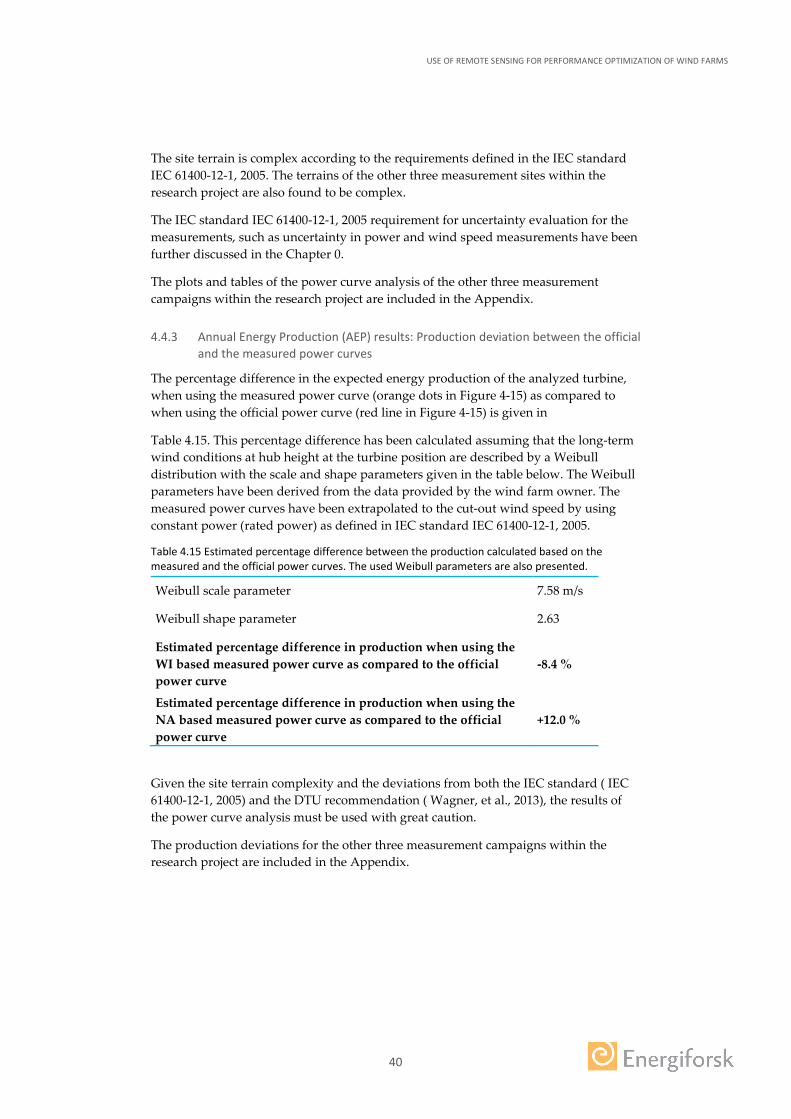
4.4.3 Annual Energy Production (AEP) results: Production deviation between the official and the measured power curves
The percentage difference in the expected energy production of the analyzed turbine, when using the measured power curve (orange dots in Figure 4-15) as compared to when using the official power curve (red line in Figure 4-15) is given in
Table 4.15. This percentage difference has been calculated assuming that the long-term wind conditions at hub height at the turbine position are described by a Weibull distribution with the scale and shape parameters given in the table below. The Weibull parameters have been derived from the data provided by the wind farm owner. The measured power curves have been extrapolated to the cut-out wind speed by using constant power (rated power) as defined in IEC standard IEC 61400-12-1, 2005.
Table 4.15 Estimated percentage difference between the production calculated based on the measured and the official power curves. The used Weibull parameters are also presented.
Weibull scale parameter 7.58 m/s
Weibull shape parameter 2.63
Estimated percentage difference in production when using the WI based measured power curve as compared to the official power curve
-8.4 %
Estimated percentage difference in production when using the NA based measured power curve as compared to the official power curve
+12.0 %
Given the site terrain complexity and the deviations from both the IEC standard ( IEC 61400-12-1, 2005) and the DTU recommendation ( Wagner, et al., 2013), the results of the power curve analysis must be used with great caution.
The production deviations for the other three measurement campaigns within the research project are included in the Appendix.

USE OF REMOTE SENSING FOR PERFORMANCE OPTIMIZATION OF WIND FARMS
41
4.5 UNCERTAINTY SOURCES
The uncertainties related to the measurements and analysis procedures presented in this research project can be reviewed in accordance with IEC standard IEC 61400-12-1, 2005 and the DTU procedure for a two beam nacelle lidar ( Wagner, et al., 2013). Moreover, additional uncertainty sources have also been listed based on the information gathered from the draft of edition 2 of the IEC standard IEC 61400-12-1, 2005 and the literature review performed within this research project.
The quantification and analysis of the uncertainties has not been covered in this research project. The topic is however briefly documented to provide guideline to future work within the same field. It has been challenging to assess the uncertainties of the chosen sites due to the complexity of roughness and terrain characteristics and due to the cold climates.
The IEC standard ( IEC 61400-12-1, 2005) follows ISO (the International Organization for Standardization) guide and evaluates uncertainties in two categories ( Ormel, 2015):
1. Category A uncertainties: which are derived from measurements
2. Category B uncertainties: which are derived from other means
4.5.1 Category A uncertainties
The category A uncertainty shall be divided into sub categories in accordance with the IEC standard ( IEC 61400-12-1, 2005) as follows:
a) Electrical power
b) Climatic variations
c) Site calibration: is planned to be included in edition 2 of the IEC standard IEC 61400-12-1, 2005.
4.5.2 Category B uncertainties
The category B uncertainty shall be divided into sub categories in accordance with the IEC standard IEC 61400-12-1, 2005 as follows:
a) Data acquisition system
b) Electrical power
c) Air density
d) Wind speed: based on DTU’s procedure for nacelle lidar, category B wind speed uncertainties can be listed as below ( Wagner, et al., 2013) :
i. Calibration uncertainty: This is derived from the lidar calibration. Based on the in-house verification performed with a reference system by the lidar manufacturer, the accuracy of in wind speed measurement has been given as 0.1 m/s and the wind direction accuracy has been given as ± 0.5°.
ii. Terrain topography: This is also referred as “flow distortion due to the terrain” and is quantified as 2 % or 3 % when the requirements of the Annex B of relevant IEC standard are complied. However, in this
USE OF REMOTE SENSING FOR PERFORMANCE OPTIMIZATION OF WIND FARMS
42
research project none of the chosen sites complies with the requirements, therefore a higher uncertainty shall be expected.
iii. Measurement height
iv. Tilt inclinometers
d) Wind Shear: is planned to be included in edition 2 of the IEC standard IEC 61400-12-1, 2005.
e) Wind veer: is planned to be included in edition 2 of the IEC standard IEC 61400-12-1, 2005.
4.5.3 Other uncertainty sources
There are additional uncertainty sources in connection to nacelle based lidar measurements and the new procedures defined in the draft of edition 2 of the IEC standard IEC 61400-12-1, 2005.
• Sensor alignment: The sensor (lidar) alignment practises of three axes (roll, tilt and yaw) during the installation introduce uncertainty in the measurements.
• As documented in the installation details at Chapter 4.1.3, the yaw alignment of Wind Iris have been adjusted to a physical reference line on the nacelle. The reference line is assumed to be parallel to the rotor axis line. However there is an uncertainty that should be taken into account which is caused by the manufacturing and assembly of nacelle structure.
• The tilt and roll alignment of the lidar have been done with the internal inclinometer built in the lidar. The accuracy of these sensors is given as ± 0.05° given by the lidar manufacturer. Moreover adjusted values have been derived from the average of at least 30 data samples.
• Uncertainty of power curves due to turbulence effects: The recently introduced turbulence normalization of power curves by PCWG and IEC standards shows that power curves are influenced by the turbulence intensity.
• Flow distortion effects on the nacelle anemometry due to presence of lidar on the nacelle: as discussed in WP3 report ( Hansson, Lindvall, & Byrkjedal, 2016).
• Uncertainty due to the absence of wind shear measurements: As it has been noted by DTU ( Wagner, et al., 2013), and this item has been planned to be included in edition 2 of the IEC standard IEC 61400-12-1, 2005 as part of wind shear uncertainty component (category B).
• Sensitivity of power curves towards seasonal changes in wind conditions: The power performance measurements performed might have seasonal dependency. An important implication of the seasonality is power performance in cold climates and has been planned to be included in edition 2 of the IEC standard IEC 61400-12-1, 2005 as an informative Annex.
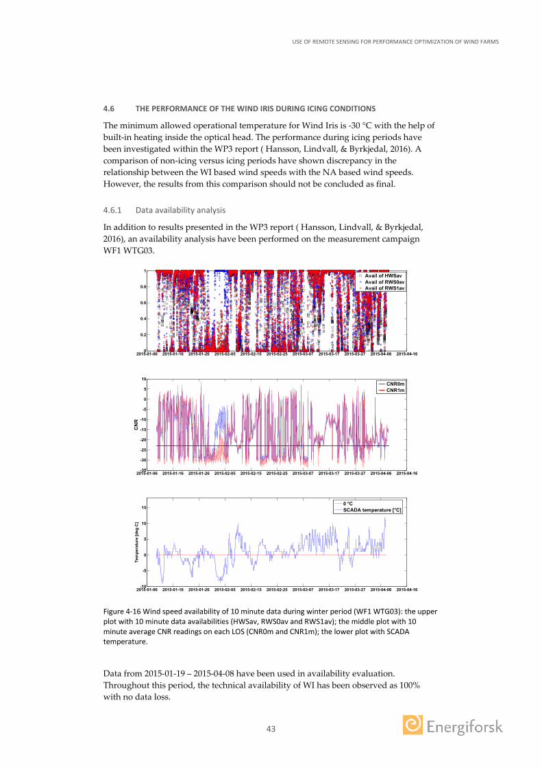
USE OF REMOTE SENSING FOR PERFORMANCE OPTIMIZATION OF WIND FARMS
43
4.6 THE PERFORMANCE OF THE WIND IRIS DURING ICING CONDITIONS
The minimum allowed operational temperature for Wind Iris is -30 °C with the help of built-in heating inside the optical head. The performance during icing periods have been investigated within the WP3 report ( Hansson, Lindvall, & Byrkjedal, 2016). A comparison of non-icing versus icing periods have shown discrepancy in the relationship between the WI based wind speeds with the NA based wind speeds. However, the results from this comparison should not be concluded as final.
4.6.1 Data availability analysis
In addition to results presented in the WP3 report ( Hansson, Lindvall, & Byrkjedal, 2016), an availability analysis have been performed on the measurement campaign WF1 WTG03.
Figure 4-16 Wind speed availability of 10 minute data during winter period (WF1 WTG03): the upper plot with 10 minute data availabilities (HWSav, RWS0av and RWS1av); the middle plot with 10 minute average CNR readings on each LOS (CNR0m and CNR1m); the lower plot with SCADA temperature.
Data from 2015-01-19 – 2015-04-08 have been used in availability evaluation. Throughout this period, the technical availability of WI has been observed as 100% with no data loss.
2015-01-06 2015-01-16 2015-01-26 2015-02-05 2015-02-15 2015-02-25 2015-03-07 2015-03-17 2015-03-27 2015-04-06 2015-04-160
0.2
0.4
0.6
0.8
1
Avail of HWSavAvail of RWS0avAvail of RWS1av
2015-01-06 2015-01-16 2015-01-26 2015-02-05 2015-02-15 2015-02-25 2015-03-07 2015-03-17 2015-03-27 2015-04-06 2015-04-16-35
-30
-25
-20
-15
-10
-5
0
5
10
CN
R
CNR0mCNR1m
2015-01-06 2015-01-16 2015-01-26 2015-02-05 2015-02-15 2015-02-25 2015-03-07 2015-03-17 2015-03-27 2015-04-06 2015-04-16-10
-5
0
5
10
15
Tem
pera
ture
[deg
C]
0 °CSCADA temperature [°C]

USE OF REMOTE SENSING FOR PERFORMANCE OPTIMIZATION OF WIND FARMS
44
As can be seen from the plots in Figure 4-16, during the first week of February 2015, the 10 minute wind speed availability on the first beam (LOS0) is low, mainly due to the CNR values below the threshold (-23 dB). During this period the temperatures at the site have been found to be below 0.0 °C almost the whole week with northerly winds. There are no neighbouring turbines or obstacles in north, so it is likely that the measurements are affected either by icing and/or snow on Wind Iris or by the local atmospheric conditions at the site. However, it is not possible to validate this, since there were no visual inspections available from the nacelle or the surrounding of the wind turbine during those times. The sensitivity to such conditions should be surveyed. These have been proposed as future work in Chapter 6.
USE OF REMOTE SENSING FOR PERFORMANCE OPTIMIZATION OF WIND FARMS
45
5 Discussion and conclusions
The main conclusions obtained in the present research are summarized below.
Chapter 2 – Causes of turbine underperformance
• Based on both the PCWG’s and other relevant literature’s conclusions, the causes of underperformance have been summarized in three main categories: wind conditions, environmental factors and wind turbine control.
Chapter 3 – Performance optimization of a wind farm
• The power curve is addressed as the main tool to assess the performance. The IEC TC 88 and the PCWG activities on analysing the power curves have been reviewed. In addition, new technologies such as use of remote sensing in power performance measurements has been considered as good alternative in validation of power curves and evaluating new optimization areas.
• The optimization measures have been summarized in two main parts as follows: Improvement of aerodynamic performance of turbine blades and control system optimization.
• As being one of the remote sensing techniques in turbine performance assessment, the most common types of nacelle based (including spinner based) remote sensing devices have been presented.
Chapter 4 - Nacelle mounted lidar as part of the performance optimization
• Four measurement campaigns at two wind farms using two wind turbines from each have been performed within this research project. The nacelle based lidar, Wind Iris, has been used in all measurement campaigns. The selected sites have moderately complex terrain with forests.
Chapter 4.2 - Yaw alignment analysis
• The yaw alignment analysis performed with collected WI and SCADA data by Kjeller Vindteknikk using in-house codes; analysis tools; and support provided by Avent Lidar Technology.
• For all four measurement campaigns, a duration of around 3 days allowed achieving a +/-0.5 ° accuracy (statistical CI) in the yaw error estimation. The calculations achieved convergence after a period about 20 days to 30 days.
• The calculated average yaw error for all four measurement campaigns are between 0° and 3.2° which corresponds to AEP gain from 0.0 % to 0.5 % respectively.
• A correction of the yaw error is not recommended for any of the selected turbines within this research project. In practice a correction shall be recommended when the average yaw error is equal to or higher than 4° which can lead to significant AEP loss.
• The scatter plots of the yaw error of all measurement campaigns show that instantaneous 10 minute mean yaw error is changing between -10° to +10° compared to the average yaw error. Therefore, energy production improvements can potentially be achieved by the control system of the turbine by keeping the rotor better aligned with the upwind flow.
• The yaw error appears to be somewhat dependent on the wind directions (nacelle yaw angle) for all four measurement campaigns. The binned sectors that are closer to the wake influenced neighbouring sectors show larger deviation than the
USE OF REMOTE SENSING FOR PERFORMANCE OPTIMIZATION OF WIND FARMS
46
average. This can also be assumed to be a result of the forested and moderately complex terrain sites or the cold climate. Therefore a frequency weighted sector bin approach could be useful in determining average yaw error, and so the potential yaw correction to apply to the turbine. This method would optimize the AEP gain is these cases.
Chapter 4.3 - Nacelle anemometer calibration analysis
• The scatter plots of WI wind speeds with NA wind speed for all measurement campaigns indicates NA measured wind speeds are generally lower than the WI measure wind speeds by 85% to 89%.
• The WI wind speeds are derived from the ranges between 2.2*D to 2.7*D which are within the accepted IEC Standard limits (from 2*D to 4*D) and are expected to have minor to none (wind turbine rotor blade) blockage effects. On the other hand terrain properties of all sites are classified as complex terrain. The measurement campaigns performed with met masts would require a site calibration procedure. In addition, the elevations in the surrounding of the selected turbines are lower than the turbine base elevation, thus the actual measurement heights are higher than the hub height of the selected turbine. As a consequence of the above mentioned aspects, the upstream lidar measured wind speed cannot automatically be assumed to be equal to the turbine wind speed.
• The analyses have also shown that there are offsets of 2˚ to 54˚ in the turbine’s definition of the north direction. It is recommended to correct these offsets in order to further increase the value of the SCADA data for production monitoring.
Chapter 4.4 - Power curve analysis
• The datasets gathered from WI and SCADA have been used to perform power curve analysis by following the guidelines given the IEC standards and DTU methodology with several deviations such as different handling of the wake filter and the exclusion of site calibration procedure.
• Just by evaluating their isolated results, three out of four measurement campaigns within this research project show turbine underperformance, while one shows turbine overperformance. The requirement of site calibration for all the measurements campaigns makes it very challenging to conclude these results. The site calibration and its uncertainties are not covered by this research project, and are therefore advised as future work.
• There are large discrepancies between the power curves derived from nacelle anemometry and the WI data based power curves. Performance assessment using power curves derived from the nacelle anemometry can be misleading, e.g. interpreted as overperformance for all measurement campaigns. The nacelle anemometry based power curve analysis is advised to be assessed by talking into account the site calibration requirements defined in the IEC Standard IEC 61400-12-2, 2013.
• Large differences (from -8% to +15%) are also found in the comparison of the AEP results from the official and the WI measured power curves. The uncertainties on the computed power curves are expected to be in the order of 6-8 % of the AEP as documented in the DTU report ( Pedersen, Gjerding, Enevoldsen, Hansen, & Jørgensen, 2002).

USE OF REMOTE SENSING FOR PERFORMANCE OPTIMIZATION OF WIND FARMS
47
Chapter 4.5 – Assessment of Uncertainties
• The quantification and analysis of the uncertainties has not been covered in this research project. The topic is however briefly documented to provide guideline to future work within the same field.
• The two uncertainty groups are listed, Category A and B, as in the IEC standard. Additional uncertainty sources have been advised to be used as guideline for future projects.
Chapter 4.6 – The performance of Wind Iris during icing conditions
• The Wind Iris has worked with good technical availability (100%) under cold climate conditions experienced during this research project.

USE OF REMOTE SENSING FOR PERFORMANCE OPTIMIZATION OF WIND FARMS
48
6 Future work and recommendations
The subject of the current research project is open to further extension with many possibilities of future research topics. Below future work has been summarized in connection to the results and experience gain within the current research project.
Installation of lidar on the nacelle
• In order to gather the optimal number of valid data samples, plan measurement campaigns in accordance with the wind regime at the site i.e. assess seasonal wind distributions and study the wind farm layout to identify wake influenced wind direction sectors of the selected wind turbine.
• Assess the operational tilt and roll angle deviation of the wind turbine prior to installation.
• Adjust pre defined range values within the lidar setups prior to installation in order to have the one of the ranges coinciding with desired measurement distance, e.g. at a distance of 2.5*D.
Yaw alignment analyses
• Perform high frequency data (1 sec) analyses e.g. as performed by several authors ( Armet, Ramirez, Simon, & Meilan, 2014) and ( Goossens, 2015) in order to investigate the sensitivity of yaw error to the averaging period.
• Define a new sampling interval for the average data in order to evaluate the yaw alignment response of the control system.
• Perform sensitivity analyses with different parameters, such as studying yaw error dependency on the wind speed and/or turbulence for all the measurement campaigns.
• Use longer measurement period campaigns and perform sensitivity analysis for seasonal effects on yaw error.
Power curve and nacelle transfer function analyses
• Adapt the power performance measurement methodology for nacelle based lidar in accordance with the 2nd Edition of the IEC standard IEC 61400-12-1, 2005 and DTU methodology ( Wagner, et al., 2013).
• Adapt PCWG’s analysis tool to perform power curve analysis with nacelle based lidar measurements.
• Evaluate the power curve for the wind direction sectors where the terrain variation is minimal or close to flat terrain conditions (non complex according to IEC standard IEC 61400-12-1, 2005).
Terrain and blockage effects
• Assess terrain and obstacles in accordance with the 2nd Edition of the IEC standard IEC 61400-12-1, 2005.
• Perform wind tunnel test to analyse the rotor blockage and terrain effects in sloped terrain or complex terrains.
• Analyse the optimal measurement distance / range selection for the lidar at a complex terrain site, e.g. “is it 2*D to 4*D (or 2.5*D)?” or “is it 1.5*D for complex terrain sites?” as estimated by Feeney et al. ( Feeney, et al., 2014).

USE OF REMOTE SENSING FOR PERFORMANCE OPTIMIZATION OF WIND FARMS
49
• Develop a numerical site calibration methodology using micro-scale wind flow models in order to estimate wind speed correction factors from the measurement location to the turbine location.
• Perform an experiment to distinguish the terrain effects from turbine rotor blockage effects on measured wind speeds as defined by Jehu et al. ( Jehu, Osler, Davoust, Morton, & Coubart-Millet, 2014). Identify periods when the turbine is operated with very low rotor RPMs or specifically stopped to increase the data coverage from lidar.
• Perform nacelle lidar based site calibration by using measurements from different ranges of the same lidar as performed by Quick ( Quick, 2013).
Other future works
• Support measurements with other remote sensing devices in order to assess complex inflow conditions e.g. vertical wind speed, turbulence, wind shear and wind veer.
• Assess uncertainty sources arisen by introducing new methodologies and use of new measurement techniques.
• Perform nacelle lidar measurements with a camera in order to record the atmospheric conditions at the site and analyze effects of atmospheric conditions on CNR values recorded by lidar as performed by Davoust et al. ( Davoust, et al., 2014) and as proposed by VTT in Finland with focus on icing ( Karlsson, Peltola, Antikainen, & Vignaroli, 2015).
USE OF REMOTE SENSING FOR PERFORMANCE OPTIMIZATION OF WIND FARMS
50
7 References
Armet, J., Ramirez, V., Simon, I., & Meilan, A. (2014). Procedure for Nacelle-Mounted LIDAR validation Conclusions on 1Hz sampling rate analysis. Barcelona: poster presented at European Wind Energy Association (EWEA) Annual Event.
Clifton, A., & Courtney, M. (2013). IEA Wind RP 15, Ground-based vertically profiling remote sensing for wind resource assessment. IEA Wind.
Davoust, S. (2013). Turbine-mounted Lidar for Performance Optimization. Stockholm: presented at Nordic Wind Power Conference: Operation & Mainteance, Avent Lidar Technology.
Davoust, S., Jehu, A., Bouillet, M., Bardon, M., Vercherin, B., Scholbrock, A., . . . Wright, A. (2014). Assessment and optimization of lidar measurement availability for turbine control. Conference Paper NREL/CP-5000-61332 presented at European Wind Energy Association Conference.
DTU Wind Energy. (2015). Windfarm Assessment Tool (WAT) Version 4.0. Roksilde, Denmark. Retrieved from http://www.wasp.dk/wat
EWEA Wind Energy Workshops. (2015). Retrieved from European Wind Energy Association Website: http://www.ewea.org/events/workshops/
Feeney, S., Derrick, A., Oram, A., Campbell, I., Hutton, G., Powles, G., . . . Burin des Roziers, E. (2014). Project Cyclops: The Way Forward in Power Curve Measurements?
Goossens, S. (2015). Field-test of nacelle-based lidar to explore its applications for Vatenfall as wind park controller. Master of Science thesis, Delft University of Technology.
Hansson, J., Lindvall, J., & Byrkjedal, Ø. (2016). Assessment and optimization of the energy production of operational wind farms, Part 3: Quantification of icing losses. Energifosk.
Harman, K. (2012). How does the real world performance of wind turbines compare with sales power curves? Lyon: Presented at EWEA Workshop: Analysis of operating wind farms, G.L. Garrad Hassan.
IEA Wind. (2015). Retrieved from The International Energy Agency (IEA) Wind, Task 32 - Lidar: http://www.forwind.de/IEAAnnex32/
IEC 61400-12-1. (2005). International standard Wind turbines - Part 12-1:Power performance measurments of electricity producing wind tubines. First edition. IEC.
IEC 61400-12-2. (2013). International standard Wind turbines - Part 12-2:Power performance measurments of electricity producing wind tubines based on nacelle anemometry. First edition. IEC.
IEC TC 88. (2015). IEC Technical Committee. Retrieved from International Electrotechnical Commission (IEC) Website: http://www.iec.ch/dyn/www/f?p=103:7:0::::FSP_ORG_ID,FSP_LANG_ID:1282,25
Jehu, A., Osler, E., Davoust, S., Morton, B., & Coubart-Millet, G. (2014). Nacelle lidar measurements in complex terrain and its application to power performance testing. Las Vegas, USA: poster presented at AWEA Wind Power Conference.
Johansson, L., Hansson, J., & Lundén, J. (2011). Elforsk report 11:20 - State of the art of wind remote sensing.
Karlsson, T., Peltola, E., Antikainen, P., & Vignaroli, A. (2015). Lidar as ice detector. presented at Winterwind.
Lindvall, J., Hansson, J., & Undheim, O. (2016). Assessment and optimization of the energy production of operational wind farms, Part 1: Post-construction production assessment. Energiforsk.
USE OF REMOTE SENSING FOR PERFORMANCE OPTIMIZATION OF WIND FARMS
51
Lopez, H. V. (2014). The Illusion of Power Curves. Master of Science Thesis, Delft University of Technology.
Marín, E. G., & Sundgaard Pedersen, H. (2014). Pointing to the right direction. Presented at EWEA Analysis of Operating Wind Farms Workshop, Malmö.
Ormel, F. (2015). Presentation of IEC Power Curve Uncertainty to PCWG. Glasgow: Vestas, presented at 11th meeting of the Power Curve Working Group.
PCWG. (2015). Retrieved from Power Curve Working Group Website: http://www.pcwg.org/
Pedersen, F. T. (2014). Update on the IEC 61400-12-1 Standard. Louisville: presented at PCWG Meeting.
Pedersen, F. T., Gjerding, S., Enevoldsen, P., Hansen, J. K., & Jørgensen, H. K. (2002). Wind turbine power performance verification in complex terrain and wind farms. Denmark. Forskningscenter Risoe. Risoe-R ; No. 1330(EN).
Peña, A., Hasager, C. B., Badger, M., Barthelmie, R. J., Bingöl, F., Cariou, J., . . . Pitter, M. (2015). Remote Sensing for Wind Energy. DTU Wind Energy.
Quick, M. (2013). A Case Study on Using a Nacelle Lidar for Power Performance Testing in Complex Terrain. DNV GL.
Schlipf, D., Kapp, S., Anger, J., Bischoff, O., Hofsäß, M., Rettenmeier, A., . . . Kühn, M. (2011). Prospects of optimization of energy production by LIDAR assisted control of wind turbines. Brussels: European Wind Energy Association Annual Event (EWEA).
Stuart, P. (2012). 1st Power Curve Working Group kick-off meeting: minutes. Retrieved from Power Curve Working Group Website: http://www.pcwg.org/proceedings/2012-12-04/WTWG-04Dec2012-Power-Curve-Working-Group-Meeting-Minutes-20121204-final.pdf
Tindal, A. (2013). Power Curve Behaviour in Energy Analysis. Dublin: presented at EWEA Resource Assesment Workshop, Session 3, Real World Power Curves.
Wagenaar, J. W., Davoust, S., Medawar, A., Coubard-Millet, G., & Boorsma, K. (2014). Turbine performance validation; the application of nacelle LiDAR. Barcelona: European Wind Energy Association (EWEA) Annual Event, ECN-M--14-017.
Wagner, R. (2010). Accounting for the speed shear in wind turbine power performance measurement. Ph.D. Thesis, Roskilde: Risø National Laboratory for Sustainable Energy. (Risø-PhD; No. 58(EN)).
Wagner, R., & Davoust, S. (2013). Nacelle lidar for power curve measurement - Avedøre campaign. DTU Wind Energy. (DTU Wind Energy E; No. 0016).
Wagner, R., Courtney, M., Friis Pedersen, T., Davoust, S., & Rivera, R. L. (2014). What makes a nacelle mounted lidar a suitable tool for power performance measurement? Barcelona: Poster session presented at European Wind Energy Conference & Exhibition.
Wagner, R., Rivera, R. L., Antoniou, I., Davoust, S., Pedersen, T. F., Courtney, M., & Diznabi, B. (2013). Procedure for wind turbine power performance measurement with a two-beam nacelle lidar. DTU Wind Energy-E-0019.
Wilkinson, M. (2014). Long-term performance of Wind Farms. Malmö: presented at EWEA Analysis of Operating Wind Farms Workshop.
WRF. (2015). Retrieved from The Weather Research & Forecasting Model Website: http://www.wrf-model.org
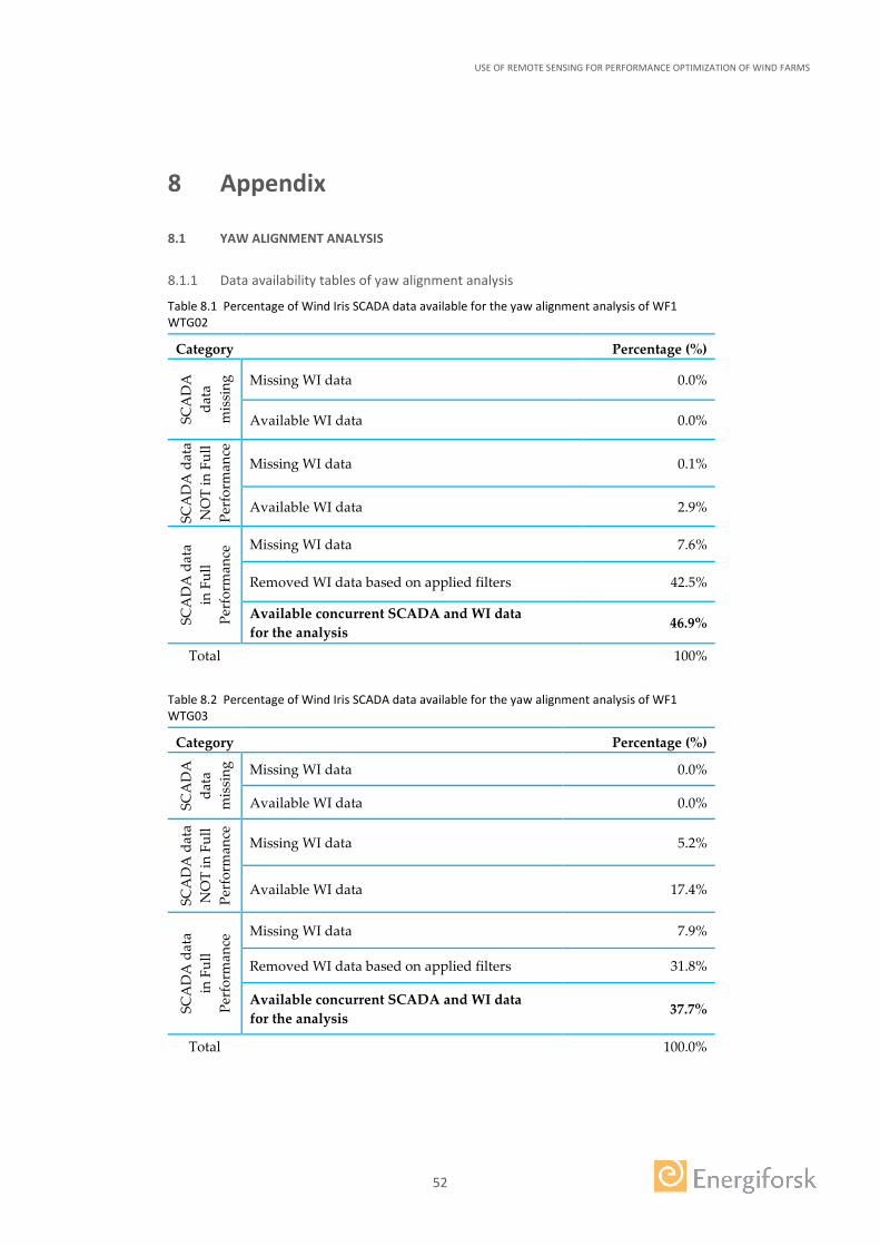
USE OF REMOTE SENSING FOR PERFORMANCE OPTIMIZATION OF WIND FARMS
52
8 Appendix
8.1 YAW ALIGNMENT ANALYSIS
8.1.1 Data availability tables of yaw alignment analysis
Table 8.1 Percentage of Wind Iris SCADA data available for the yaw alignment analysis of WF1 WTG02
Category Percentage (%)
SCA
DA
da
ta
mis
sing
Missing WI data 0.0%
Available WI data 0.0%
SCA
DA
dat
a N
OT
in F
ull
Perf
orm
ance
Missing WI data 0.1%
Available WI data 2.9%
SCA
DA
dat
a
in F
ull
Perf
orm
ance
Missing WI data 7.6%
Removed WI data based on applied filters 42.5%
Available concurrent SCADA and WI data for the analysis
46.9%
Total 100%
Table 8.2 Percentage of Wind Iris SCADA data available for the yaw alignment analysis of WF1 WTG03
Category Percentage (%)
SCA
DA
da
ta
mis
sing
Missing WI data 0.0%
Available WI data 0.0%
SCA
DA
dat
a N
OT
in F
ull
Perf
orm
ance
Missing WI data 5.2%
Available WI data 17.4%
SCA
DA
dat
a
in F
ull
Perf
orm
ance
Missing WI data 7.9%
Removed WI data based on applied filters 31.8%
Available concurrent SCADA and WI data for the analysis 37.7%
Total 100.0%
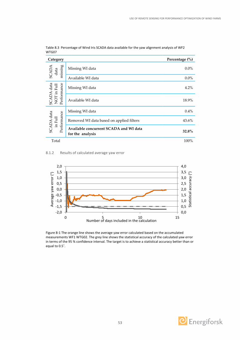
USE OF REMOTE SENSING FOR PERFORMANCE OPTIMIZATION OF WIND FARMS
53
Table 8.3 Percentage of Wind Iris SCADA data available for the yaw alignment analysis of WF2 WTG07
Category Percentage (%)
SCA
DA
da
ta
mis
sing
Missing WI data 0.0%
Available WI data 0.0%
SCA
DA
dat
a N
OT
in F
ull
Perf
orm
ance
Missing WI data 4.2%
Available WI data 18.9%
SCA
DA
dat
a
in F
ull
Perf
orm
ance
Missing WI data 0.4%
Removed WI data based on applied filters 43.6%
Available concurrent SCADA and WI data for the analysis 32.8%
Total 100%
8.1.2 Results of calculated average yaw error
Figure 8-1 The orange line shows the average yaw error calculated based on the accumulated measurements WF1 WTG02. The grey line shows the statistical accuracy of the calculated yaw error in terms of the 95 % confidence interval. The target is to achieve a statistical accuracy better than or equal to 0.5˚.
0,00,51,01,52,02,53,03,54,0
-2,0-1,5-1,0-0,50,00,51,01,52,0
0 5 10 15
Stat
istic
al a
ccur
acy
(°)
Aver
age
yaw
err
or (°
)
Number of days included in the calculation
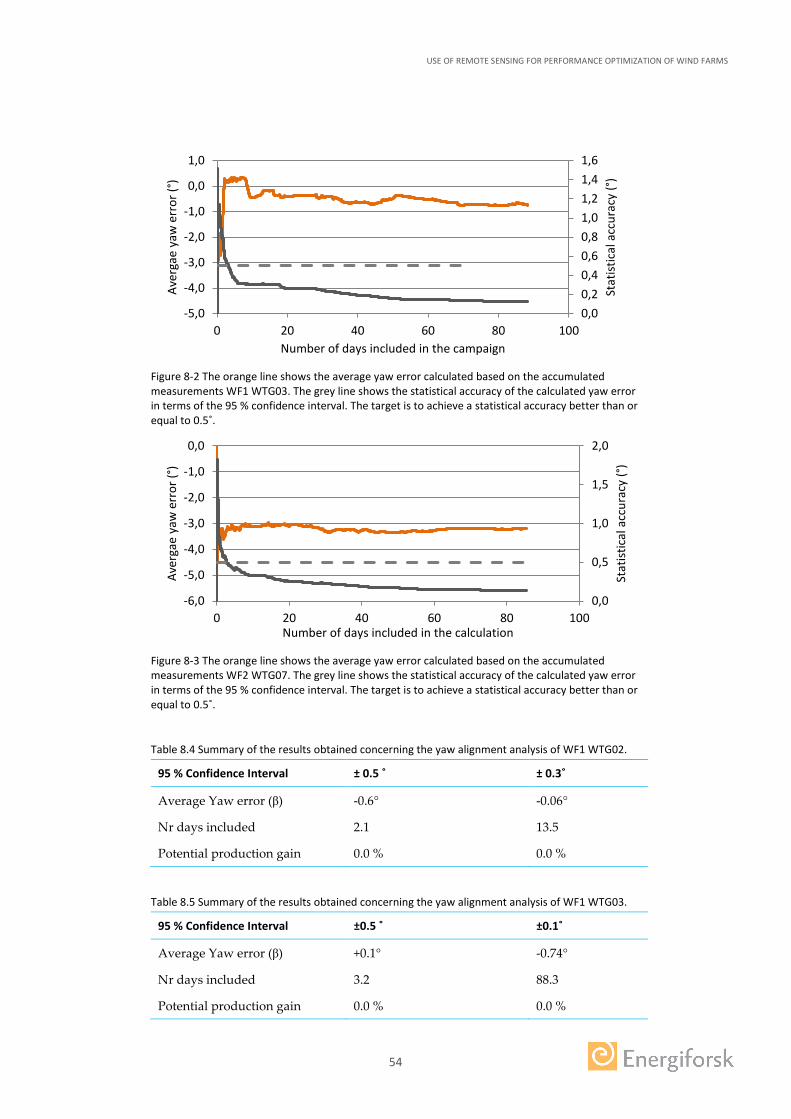
USE OF REMOTE SENSING FOR PERFORMANCE OPTIMIZATION OF WIND FARMS
54
Figure 8-2 The orange line shows the average yaw error calculated based on the accumulated measurements WF1 WTG03. The grey line shows the statistical accuracy of the calculated yaw error in terms of the 95 % confidence interval. The target is to achieve a statistical accuracy better than or equal to 0.5˚.
Figure 8-3 The orange line shows the average yaw error calculated based on the accumulated measurements WF2 WTG07. The grey line shows the statistical accuracy of the calculated yaw error in terms of the 95 % confidence interval. The target is to achieve a statistical accuracy better than or equal to 0.5˚.
Table 8.4 Summary of the results obtained concerning the yaw alignment analysis of WF1 WTG02.
95 % Confidence Interval ± 0.5 ˚ ± 0.3˚
Average Yaw error (β) -0.6° -0.06°
Nr days included 2.1 13.5
Potential production gain 0.0 % 0.0 %
Table 8.5 Summary of the results obtained concerning the yaw alignment analysis of WF1 WTG03.
95 % Confidence Interval ±0.5 ˚ ±0.1˚
Average Yaw error (β) +0.1° -0.74°
Nr days included 3.2 88.3
Potential production gain 0.0 % 0.0 %
0,00,20,40,60,81,01,21,41,6
-5,0
-4,0
-3,0
-2,0
-1,0
0,0
1,0
0 20 40 60 80 100
Stat
istic
al a
ccur
acy
(°)
Aver
gae
yaw
err
or (°
)
Number of days included in the campaign
0,0
0,5
1,0
1,5
2,0
-6,0
-5,0
-4,0
-3,0
-2,0
-1,0
0,0
0 20 40 60 80 100St
atist
ical
acc
urac
y (°
)
Aver
gae
yaw
err
or (°
)
Number of days included in the calculation
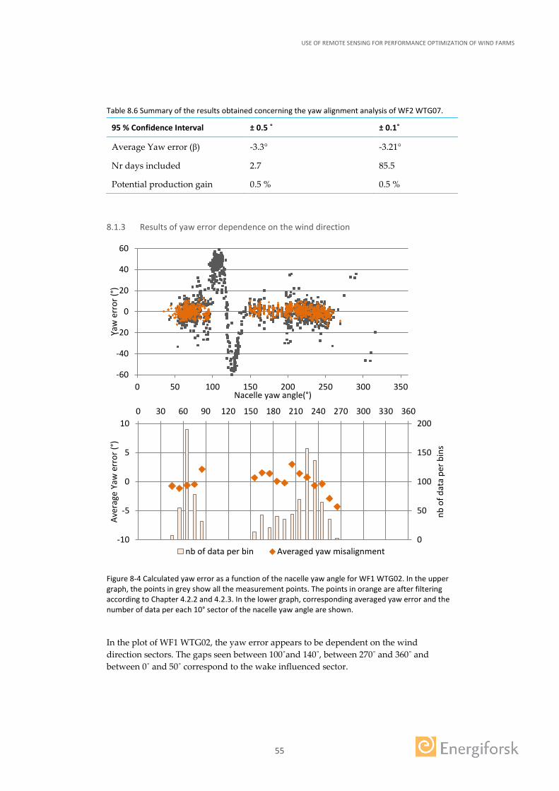
USE OF REMOTE SENSING FOR PERFORMANCE OPTIMIZATION OF WIND FARMS
55
Table 8.6 Summary of the results obtained concerning the yaw alignment analysis of WF2 WTG07.
95 % Confidence Interval ± 0.5 ˚ ± 0.1˚
Average Yaw error (β) -3.3° -3.21°
Nr days included 2.7 85.5
Potential production gain 0.5 % 0.5 %
8.1.3 Results of yaw error dependence on the wind direction
Figure 8-4 Calculated yaw error as a function of the nacelle yaw angle for WF1 WTG02. In the upper graph, the points in grey show all the measurement points. The points in orange are after filtering according to Chapter 4.2.2 and 4.2.3. In the lower graph, corresponding averaged yaw error and the number of data per each 10° sector of the nacelle yaw angle are shown.
In the plot of WF1 WTG02, the yaw error appears to be dependent on the wind direction sectors. The gaps seen between 100˚and 140˚, between 270˚ and 360˚ and between 0˚ and 50˚ correspond to the wake influenced sector.
-60
-40
-20
0
20
40
60
0 50 100 150 200 250 300 350
Yaw
err
or (°
)
Nacelle yaw angle(°)
0
50
100
150
200
-10
-5
0
5
100 30 60 90 120 150 180 210 240 270 300 330 360
nb o
f dat
a pe
r bin
s
Aver
age
Yaw
err
or (°
)
nb of data per bin Averaged yaw misalignment
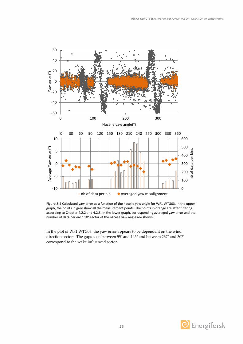
USE OF REMOTE SENSING FOR PERFORMANCE OPTIMIZATION OF WIND FARMS
56
Figure 8-5 Calculated yaw error as a function of the nacelle yaw angle for WF1 WTG03. In the upper graph, the points in grey show all the measurement points. The points in orange are after filtering according to Chapter 4.2.2 and 4.2.3. In the lower graph, corresponding averaged yaw error and the number of data per each 10° sector of the nacelle yaw angle are shown.
In the plot of WF1 WTG03, the yaw error appears to be dependent on the wind direction sectors. The gaps seen between 55˚ and 145˚ and between 267˚ and 307˚ correspond to the wake influenced sector.
-60
-40
-20
0
20
40
60
0 100 200 300
Yaw
err
or (°
)
Nacelle yaw angle(°)
0
100
200
300
400
500
600
-10
-5
0
5
100 30 60 90 120 150 180 210 240 270 300 330 360
nb o
f dat
a pe
r bin
s
Aver
age
Yaw
err
or (°
)
nb of data per bin Averaged yaw misalignment
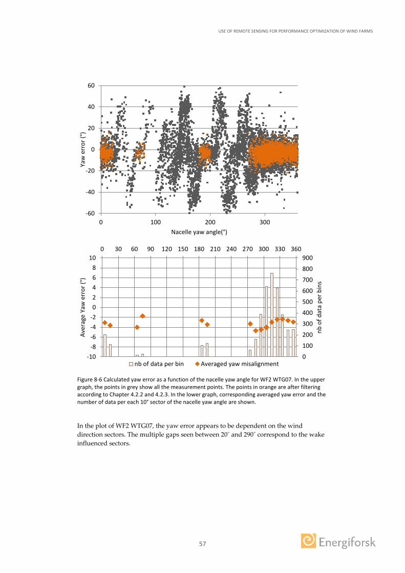
USE OF REMOTE SENSING FOR PERFORMANCE OPTIMIZATION OF WIND FARMS
57
Figure 8-6 Calculated yaw error as a function of the nacelle yaw angle for WF2 WTG07. In the upper graph, the points in grey show all the measurement points. The points in orange are after filtering according to Chapter 4.2.2 and 4.2.3. In the lower graph, corresponding averaged yaw error and the number of data per each 10° sector of the nacelle yaw angle are shown.
In the plot of WF2 WTG07, the yaw error appears to be dependent on the wind direction sectors. The multiple gaps seen between 20˚ and 290˚ correspond to the wake influenced sectors.
-60
-40
-20
0
20
40
60
0 100 200 300
Yaw
err
or (°
)
Nacelle yaw angle(°)
0
100
200
300
400
500
600
700
800
900
-10-8-6-4-202468
100 30 60 90 120 150 180 210 240 270 300 330 360
nb o
f dat
a pe
r bin
s
Aver
age
Yaw
err
or (°
)
nb of data per bin Averaged yaw misalignment
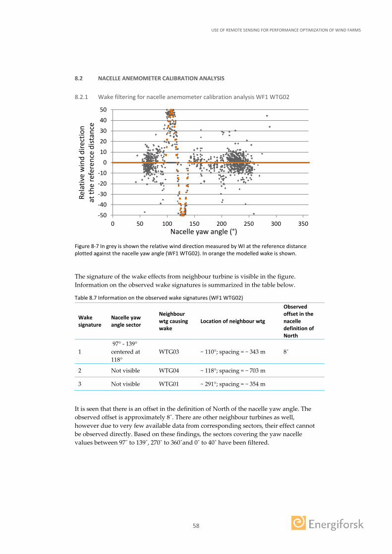
USE OF REMOTE SENSING FOR PERFORMANCE OPTIMIZATION OF WIND FARMS
58
8.2 NACELLE ANEMOMETER CALIBRATION ANALYSIS
8.2.1 Wake filtering for nacelle anemometer calibration analysis WF1 WTG02
Figure 8-7 In grey is shown the relative wind direction measured by WI at the reference distance plotted against the nacelle yaw angle (WF1 WTG02). In orange the modelled wake is shown.
The signature of the wake effects from neighbour turbine is visible in the figure. Information on the observed wake signatures is summarized in the table below.
Table 8.7 Information on the observed wake signatures (WF1 WTG02)
Wake signature
Nacelle yaw angle sector
Neighbour wtg causing wake
Location of neighbour wtg
Observed offset in the nacelle definition of North
1 97° - 139° centered at 118°
WTG03 ~ 110°; spacing = ~ 343 m 8˚
2 Not visible WTG04 ~ 118°; spacing = ~ 703 m
3 Not visible WTG01 ~ 291°; spacing = ~ 354 m
It is seen that there is an offset in the definition of North of the nacelle yaw angle. The observed offset is approximately 8˚. There are other neighbour turbines as well, however due to very few available data from corresponding sectors, their effect cannot be observed directly. Based on these findings, the sectors covering the yaw nacelle values between 97˚ to 139˚, 270˚ to 360˚and 0˚ to 40˚ have been filtered.
-50
-40
-30
-20
-10
0
10
20
30
40
50
0 50 100 150 200 250 300 350
Rela
tive
win
d di
rect
ion
at th
e re
fere
nce
dist
ance
Nacelle yaw angle (°)
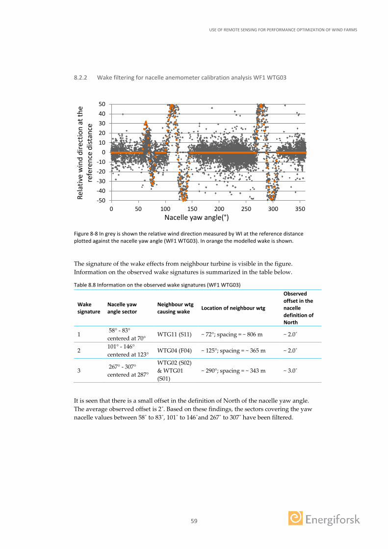
USE OF REMOTE SENSING FOR PERFORMANCE OPTIMIZATION OF WIND FARMS
59
8.2.2 Wake filtering for nacelle anemometer calibration analysis WF1 WTG03
Figure 8-8 In grey is shown the relative wind direction measured by WI at the reference distance plotted against the nacelle yaw angle (WF1 WTG03). In orange the modelled wake is shown.
The signature of the wake effects from neighbour turbine is visible in the figure. Information on the observed wake signatures is summarized in the table below.
Table 8.8 Information on the observed wake signatures (WF1 WTG03)
Wake signature
Nacelle yaw angle sector
Neighbour wtg causing wake Location of neighbour wtg
Observed offset in the nacelle definition of North
1 58° - 83° centered at 70°
WTG11 (S11) ~ 72°; spacing = ~ 806 m ~ 2.0˚
2 101° - 146° centered at 123°
WTG04 (F04) ~ 125°; spacing = ~ 365 m ~ 2.0˚
3 267° - 307° centered at 287°
WTG02 (S02) & WTG01 (S01)
~ 290°; spacing = ~ 343 m ~ 3.0˚
It is seen that there is a small offset in the definition of North of the nacelle yaw angle. The average observed offset is 2˚. Based on these findings, the sectors covering the yaw nacelle values between 58˚ to 83˚, 101˚ to 146˚and 267˚ to 307˚ have been filtered.
-50-40-30-20-10
01020304050
0 50 100 150 200 250 300 350
Rela
tive
win
d di
rect
ion
at th
e re
fere
nce
dist
ance
Nacelle yaw angle(°)
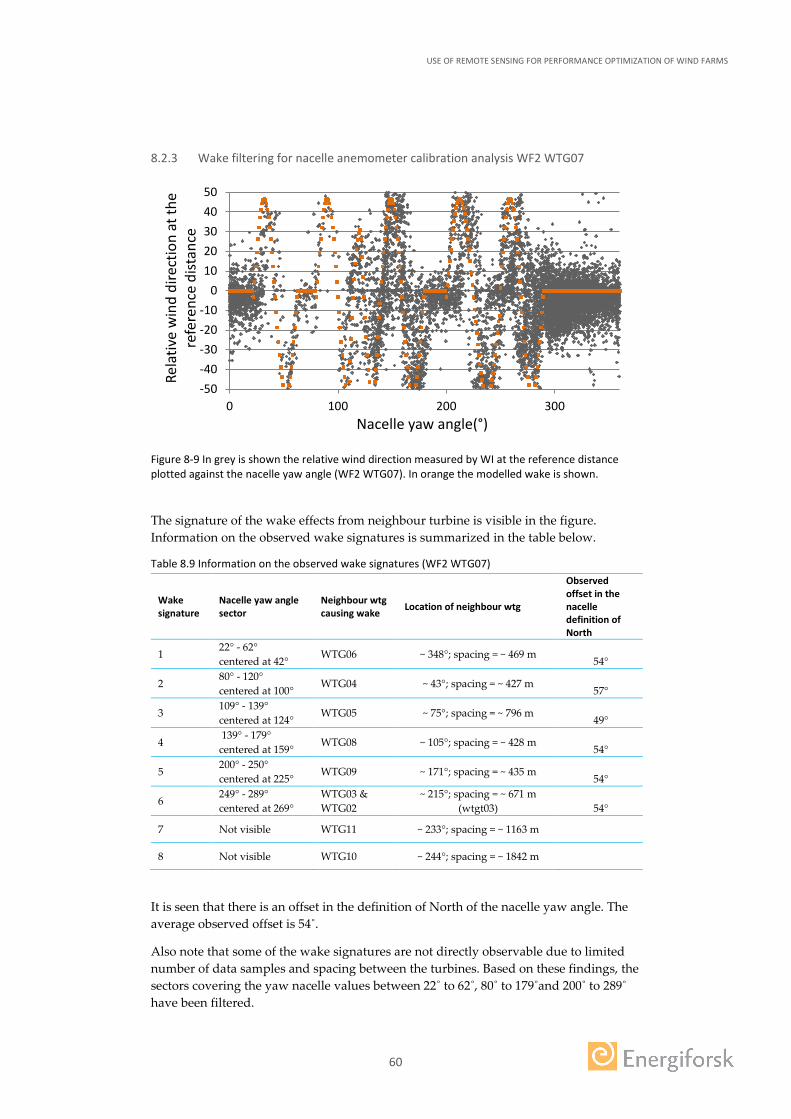
USE OF REMOTE SENSING FOR PERFORMANCE OPTIMIZATION OF WIND FARMS
60
8.2.3 Wake filtering for nacelle anemometer calibration analysis WF2 WTG07
Figure 8-9 In grey is shown the relative wind direction measured by WI at the reference distance plotted against the nacelle yaw angle (WF2 WTG07). In orange the modelled wake is shown.
The signature of the wake effects from neighbour turbine is visible in the figure. Information on the observed wake signatures is summarized in the table below.
Table 8.9 Information on the observed wake signatures (WF2 WTG07)
Wake signature
Nacelle yaw angle sector
Neighbour wtg causing wake Location of neighbour wtg
Observed offset in the nacelle definition of North
1 22° - 62° centered at 42°
WTG06 ~ 348°; spacing = ~ 469 m 54°
2 80° - 120° centered at 100°
WTG04 ~ 43°; spacing = ~ 427 m 57°
3 109° - 139° centered at 124°
WTG05 ~ 75°; spacing = ~ 796 m 49°
4 139° - 179° centered at 159°
WTG08 ~ 105°; spacing = ~ 428 m 54°
5 200° - 250° centered at 225°
WTG09 ~ 171°; spacing = ~ 435 m 54°
6 249° - 289° centered at 269°
WTG03 & WTG02
~ 215°; spacing = ~ 671 m (wtgt03) 54°
7 Not visible WTG11 ~ 233°; spacing = ~ 1163 m
8 Not visible WTG10 ~ 244°; spacing = ~ 1842 m
It is seen that there is an offset in the definition of North of the nacelle yaw angle. The average observed offset is 54˚.
Also note that some of the wake signatures are not directly observable due to limited number of data samples and spacing between the turbines. Based on these findings, the sectors covering the yaw nacelle values between 22˚ to 62˚, 80˚ to 179˚and 200˚ to 289˚ have been filtered.
-50-40-30-20-10
01020304050
0 100 200 300
Rela
tive
win
d di
rect
ion
at th
e re
fere
nce
dist
ance
Nacelle yaw angle(°)
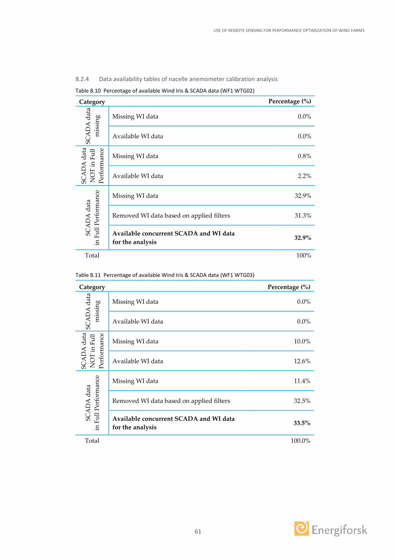
USE OF REMOTE SENSING FOR PERFORMANCE OPTIMIZATION OF WIND FARMS
61
8.2.4 Data availability tables of nacelle anemometer calibration analysis
Table 8.10 Percentage of available Wind Iris & SCADA data (WF1 WTG02)
Category Percentage (%)
SCA
DA
dat
a m
issi
ng Missing WI data 0.0%
Available WI data 0.0%
SCA
DA
dat
a N
OT
in F
ull
Perf
orm
ance
Missing WI data 0.8%
Available WI data 2.2%
SCA
DA
dat
a
in F
ull P
erfo
rman
ce
Missing WI data 32.9%
Removed WI data based on applied filters 31.3%
Available concurrent SCADA and WI data for the analysis 32.9%
Total 100%
Table 8.11 Percentage of available Wind Iris & SCADA data (WF1 WTG03)
Category Percentage (%)
SCA
DA
dat
a m
issi
ng Missing WI data 0.0%
Available WI data 0.0%
SCA
DA
dat
a N
OT
in F
ull
Perf
orm
ance
Missing WI data 10.0%
Available WI data 12.6%
SCA
DA
dat
a
in F
ull P
erfo
rman
ce
Missing WI data 11.4%
Removed WI data based on applied filters 32.5%
Available concurrent SCADA and WI data for the analysis 33.5%
Total 100.0%
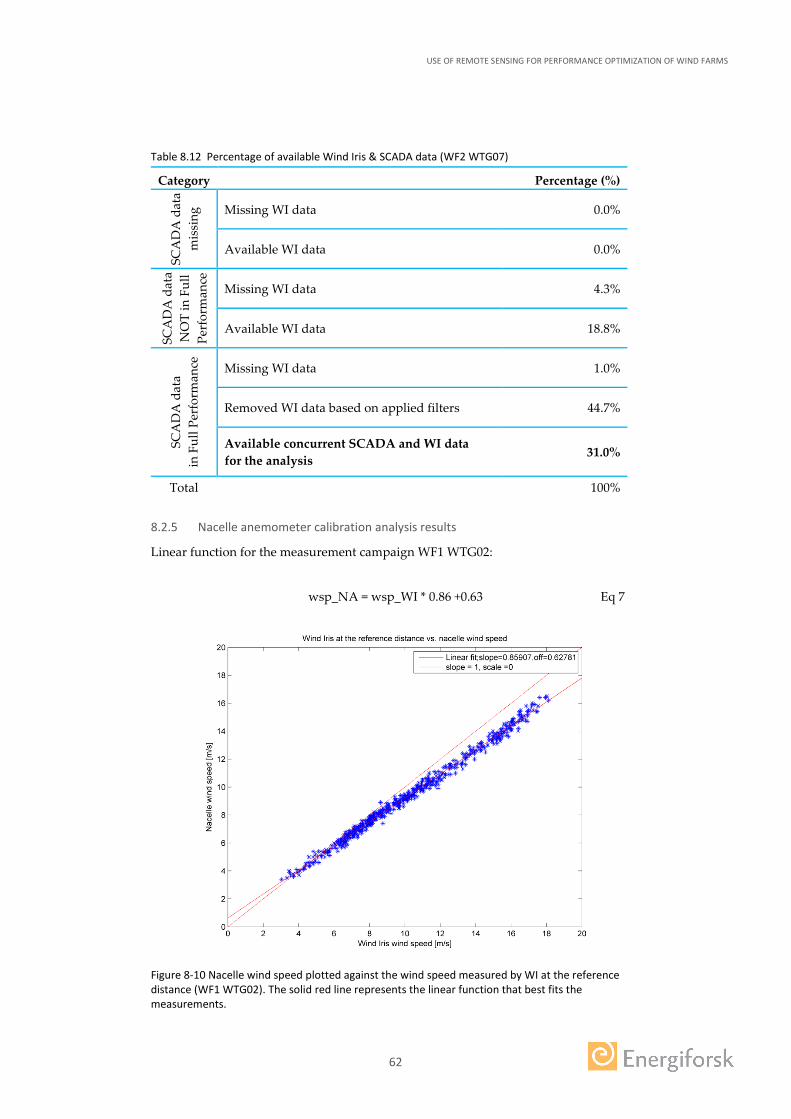
USE OF REMOTE SENSING FOR PERFORMANCE OPTIMIZATION OF WIND FARMS
62
Table 8.12 Percentage of available Wind Iris & SCADA data (WF2 WTG07)
Category Percentage (%) SC
AD
A d
ata
mis
sing
Missing WI data 0.0%
Available WI data 0.0%
SCA
DA
dat
a N
OT
in F
ull
Perf
orm
ance
Missing WI data 4.3%
Available WI data 18.8%
SCA
DA
dat
a
in F
ull P
erfo
rman
ce
Missing WI data 1.0%
Removed WI data based on applied filters 44.7%
Available concurrent SCADA and WI data for the analysis 31.0%
Total 100%
8.2.5 Nacelle anemometer calibration analysis results
Linear function for the measurement campaign WF1 WTG02:
wsp_NA = wsp_WI * 0.86 +0.63 Eq 7
Figure 8-10 Nacelle wind speed plotted against the wind speed measured by WI at the reference distance (WF1 WTG02). The solid red line represents the linear function that best fits the measurements.
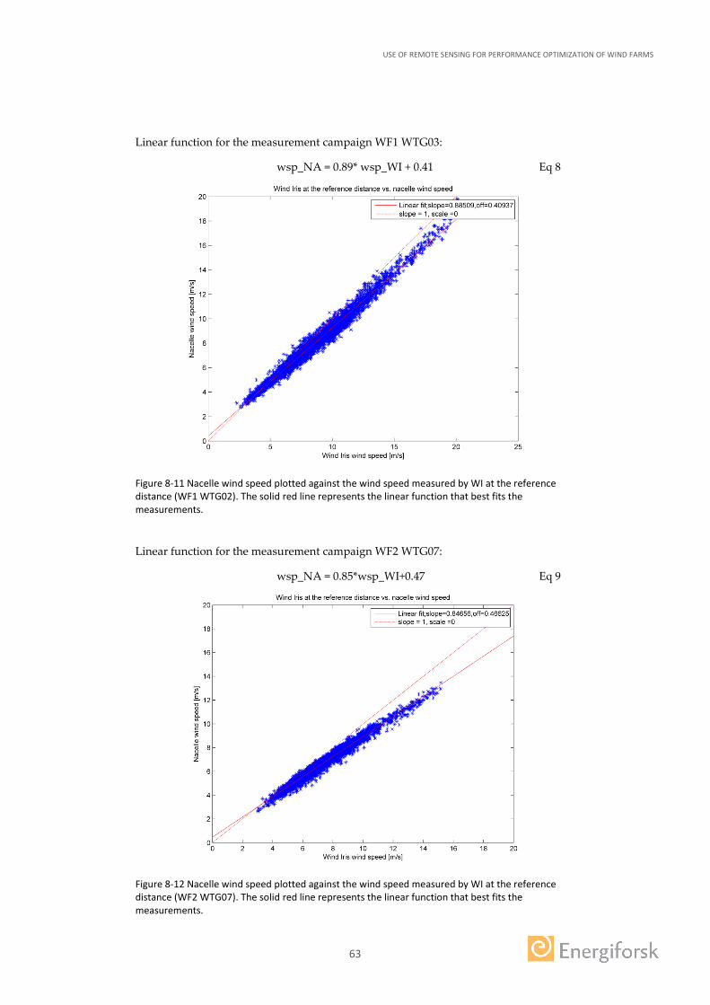
USE OF REMOTE SENSING FOR PERFORMANCE OPTIMIZATION OF WIND FARMS
63
Linear function for the measurement campaign WF1 WTG03:
wsp_NA = 0.89* wsp_WI + 0.41 Eq 8
Figure 8-11 Nacelle wind speed plotted against the wind speed measured by WI at the reference distance (WF1 WTG02). The solid red line represents the linear function that best fits the measurements.
Linear function for the measurement campaign WF2 WTG07:
wsp_NA = 0.85*wsp_WI+0.47 Eq 9
Figure 8-12 Nacelle wind speed plotted against the wind speed measured by WI at the reference distance (WF2 WTG07). The solid red line represents the linear function that best fits the measurements.
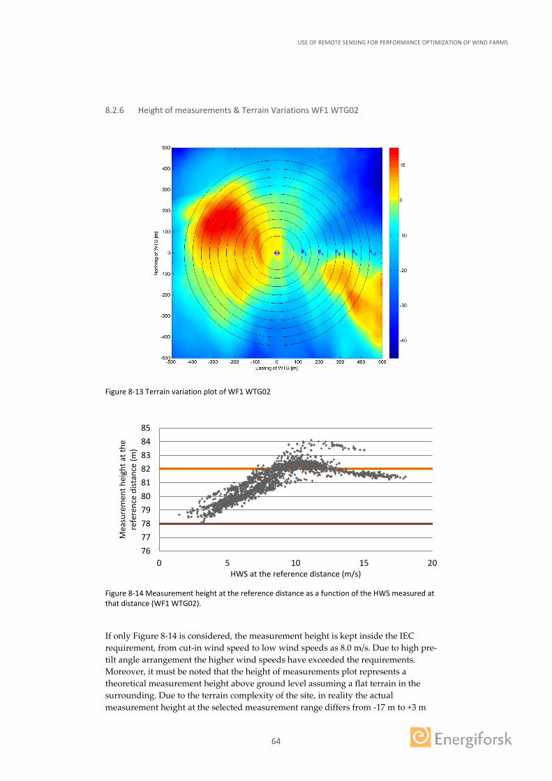
USE OF REMOTE SENSING FOR PERFORMANCE OPTIMIZATION OF WIND FARMS
64
8.2.6 Height of measurements & Terrain Variations WF1 WTG02
Figure 8-13 Terrain variation plot of WF1 WTG02
Figure 8-14 Measurement height at the reference distance as a function of the HWS measured at that distance (WF1 WTG02).
If only Figure 8-14 is considered, the measurement height is kept inside the IEC requirement, from cut-in wind speed to low wind speeds as 8.0 m/s. Due to high pre-tilt angle arrangement the higher wind speeds have exceeded the requirements. Moreover, it must be noted that the height of measurements plot represents a theoretical measurement height above ground level assuming a flat terrain in the surrounding. Due to the terrain complexity of the site, in reality the actual measurement height at the selected measurement range differs from -17 m to +3 m
76777879808182838485
0 5 10 15 20
Mea
sure
men
t hei
ght a
t the
re
fere
nce
dist
ance
(m)
HWS at the reference distance (m/s)
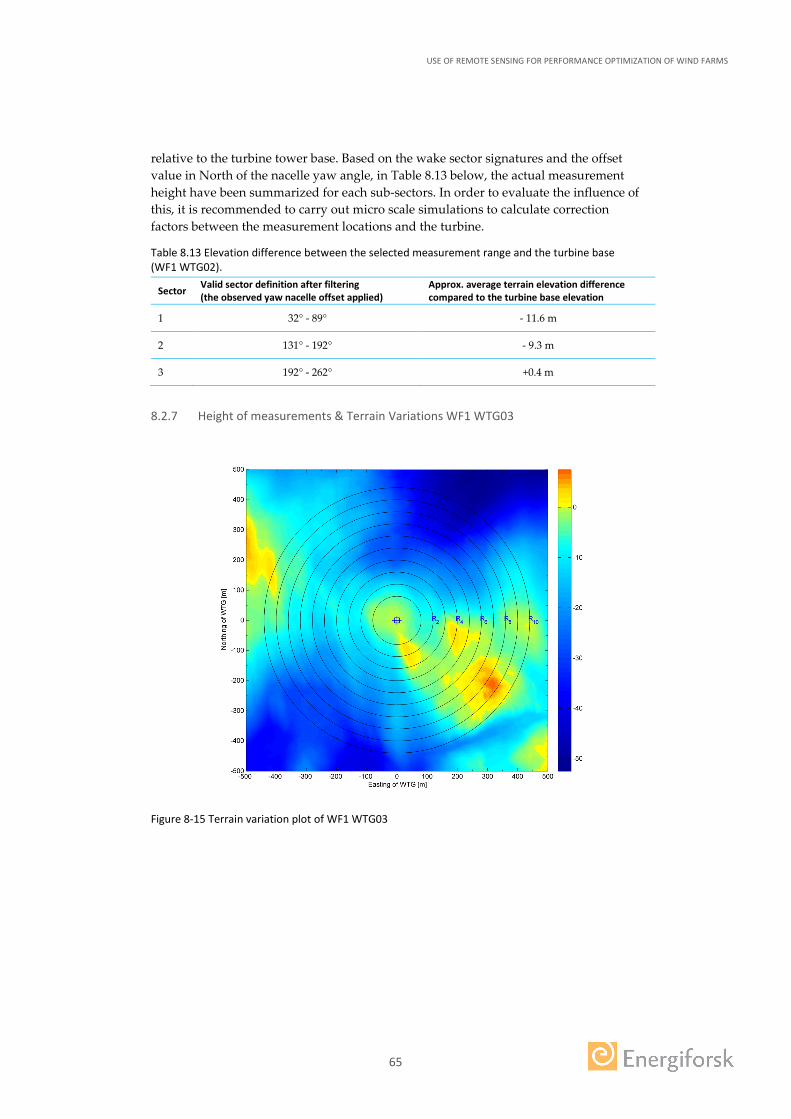
USE OF REMOTE SENSING FOR PERFORMANCE OPTIMIZATION OF WIND FARMS
65
relative to the turbine tower base. Based on the wake sector signatures and the offset value in North of the nacelle yaw angle, in Table 8.13 below, the actual measurement height have been summarized for each sub-sectors. In order to evaluate the influence of this, it is recommended to carry out micro scale simulations to calculate correction factors between the measurement locations and the turbine.
Table 8.13 Elevation difference between the selected measurement range and the turbine base (WF1 WTG02).
Sector Valid sector definition after filtering (the observed yaw nacelle offset applied)
Approx. average terrain elevation difference compared to the turbine base elevation
1 32° - 89° - 11.6 m
2 131° - 192° - 9.3 m
3 192° - 262° +0.4 m
8.2.7 Height of measurements & Terrain Variations WF1 WTG03
Figure 8-15 Terrain variation plot of WF1 WTG03
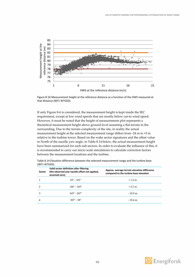
USE OF REMOTE SENSING FOR PERFORMANCE OPTIMIZATION OF WIND FARMS
66
Figure 8-16 Measurement height at the reference distance as a function of the HWS measured at that distance (WF1 WTG03).
If only Figure 8-6 is considered, the measurement height is kept inside the IEC requirement, except at low wind speeds that are mostly below cut-in wind speed. However, it must be noted that the height of measurements plot represents a theoretical measurement height above ground level assuming a flat terrain in the surrounding. Due to the terrain complexity of the site, in reality the actual measurement height at the selected measurement range differs from -24 m to +5 m relative to the turbine tower. Based on the wake sector signatures and the offset value in North of the nacelle yaw angle, in Table 8.14 below, the actual measurement height have been summarized for each sub-sectors. In order to evaluate the influence of this, it is recommended to carry out micro scale simulations to calculate correction factors between the measurement locations and the turbine.
Table 8.14 Elevation difference between the selected measurement range and the turbine base (WF1 WTG03).
Sector Valid sector definition after filtering (the observed yaw nacelle offset not applied, assumed zero)
Approx. average terrain elevation difference compared to the turbine base elevation
1 83° - 101° + 1.2 m
2 146° - 165° + 2.2 m
3 165° - 267° - 10.0 m
4 307° - 58° - 18.4 m
7576777879808182838485
1 6 11 16 21
Mea
sure
men
t hei
ght a
t the
re
fere
nce
dist
ance
(m)
HWS at the reference distance (m/s)
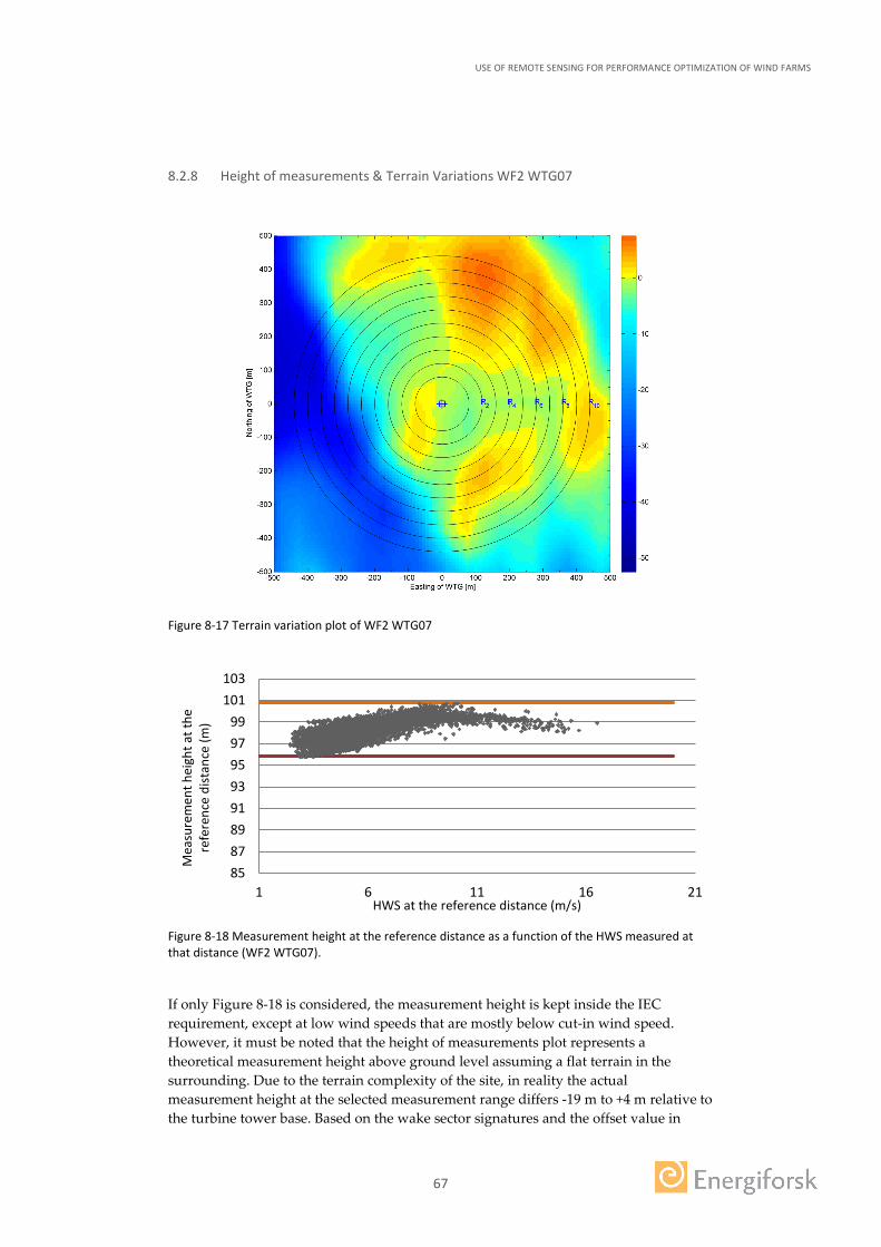
USE OF REMOTE SENSING FOR PERFORMANCE OPTIMIZATION OF WIND FARMS
67
8.2.8 Height of measurements & Terrain Variations WF2 WTG07
Figure 8-17 Terrain variation plot of WF2 WTG07
Figure 8-18 Measurement height at the reference distance as a function of the HWS measured at that distance (WF2 WTG07).
If only Figure 8-18 is considered, the measurement height is kept inside the IEC requirement, except at low wind speeds that are mostly below cut-in wind speed. However, it must be noted that the height of measurements plot represents a theoretical measurement height above ground level assuming a flat terrain in the surrounding. Due to the terrain complexity of the site, in reality the actual measurement height at the selected measurement range differs -19 m to +4 m relative to the turbine tower base. Based on the wake sector signatures and the offset value in
8587899193959799
101103
1 6 11 16 21
Mea
sure
men
t hei
ght a
t the
re
fere
nce
dist
ance
(m)
HWS at the reference distance (m/s)
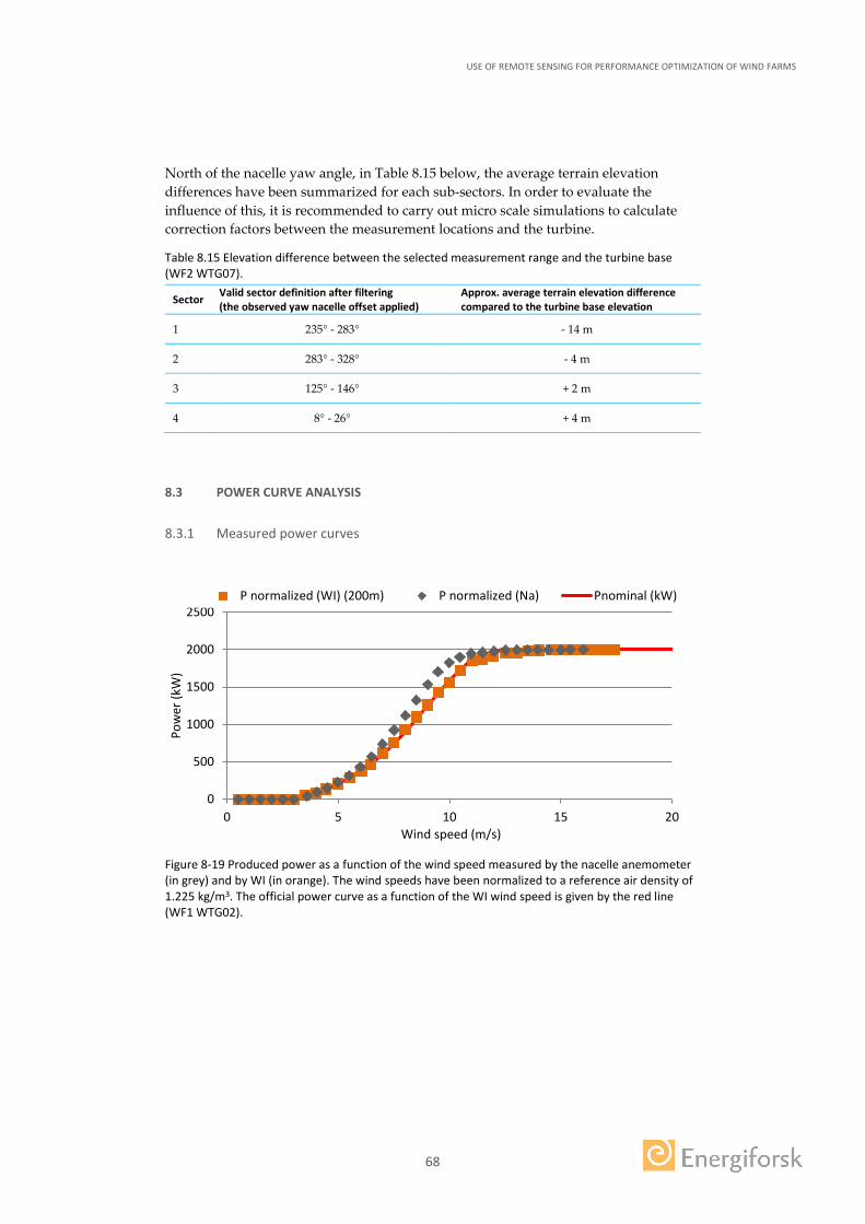
USE OF REMOTE SENSING FOR PERFORMANCE OPTIMIZATION OF WIND FARMS
68
North of the nacelle yaw angle, in Table 8.15 below, the average terrain elevation differences have been summarized for each sub-sectors. In order to evaluate the influence of this, it is recommended to carry out micro scale simulations to calculate correction factors between the measurement locations and the turbine.
Table 8.15 Elevation difference between the selected measurement range and the turbine base (WF2 WTG07).
Sector Valid sector definition after filtering (the observed yaw nacelle offset applied)
Approx. average terrain elevation difference compared to the turbine base elevation
1 235° - 283° - 14 m
2 283° - 328° - 4 m
3 125° - 146° + 2 m
4 8° - 26° + 4 m
8.3 POWER CURVE ANALYSIS
8.3.1 Measured power curves
Figure 8-19 Produced power as a function of the wind speed measured by the nacelle anemometer (in grey) and by WI (in orange). The wind speeds have been normalized to a reference air density of 1.225 kg/m3. The official power curve as a function of the WI wind speed is given by the red line (WF1 WTG02).
0
500
1000
1500
2000
2500
0 5 10 15 20
Pow
er (k
W)
Wind speed (m/s)
P normalized (WI) (200m) P normalized (Na) Pnominal (kW)
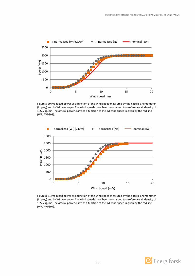
USE OF REMOTE SENSING FOR PERFORMANCE OPTIMIZATION OF WIND FARMS
69
Figure 8-20 Produced power as a function of the wind speed measured by the nacelle anemometer (in grey) and by WI (in orange). The wind speeds have been normalized to a reference air density of 1.225 kg/m3. The official power curve as a function of the WI wind speed is given by the red line (WF1 WTG03).
Figure 8-21 Produced power as a function of the wind speed measured by the nacelle anemometer (in grey) and by WI (in orange). The wind speeds have been normalized to a reference air density of 1.225 kg/m3. The official power curve as a function of the WI wind speed is given by the red line (WF2 WTG07).
0
500
1000
1500
2000
2500
0 5 10 15 20
Pow
er (k
W)
Wind speed (m/s)
P normalized (WI) (200m) P normalized (Na) Pnominal (kW)
0
500
1000
1500
2000
2500
3000
0 5 10 15 20
POW
ER (k
W)
Wind Speed (m/s)
P normalized (WI) (240m) P normalized (Na) Pnominal (kW)
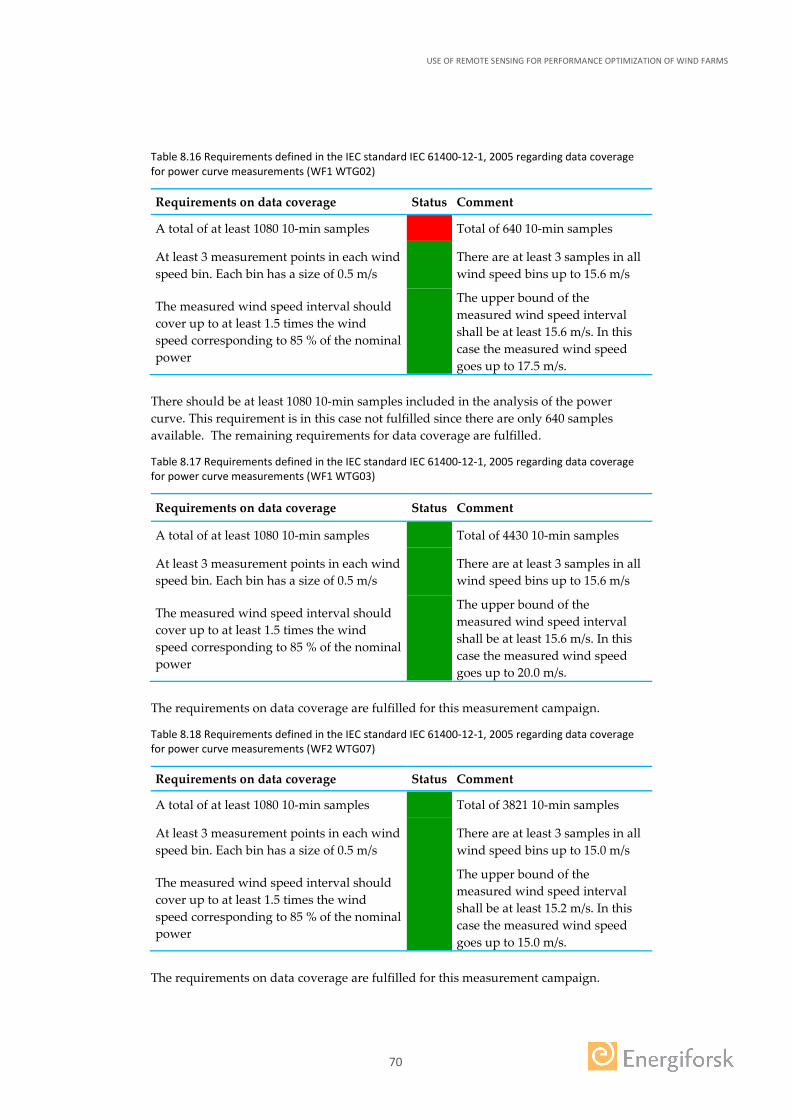
USE OF REMOTE SENSING FOR PERFORMANCE OPTIMIZATION OF WIND FARMS
70
Table 8.16 Requirements defined in the IEC standard IEC 61400-12-1, 2005 regarding data coverage for power curve measurements (WF1 WTG02)
Requirements on data coverage Status Comment
A total of at least 1080 10-min samples Total of 640 10-min samples
At least 3 measurement points in each wind speed bin. Each bin has a size of 0.5 m/s
There are at least 3 samples in all wind speed bins up to 15.6 m/s
The measured wind speed interval should cover up to at least 1.5 times the wind speed corresponding to 85 % of the nominal power
The upper bound of the measured wind speed interval shall be at least 15.6 m/s. In this case the measured wind speed goes up to 17.5 m/s.
There should be at least 1080 10-min samples included in the analysis of the power curve. This requirement is in this case not fulfilled since there are only 640 samples available. The remaining requirements for data coverage are fulfilled.
Table 8.17 Requirements defined in the IEC standard IEC 61400-12-1, 2005 regarding data coverage for power curve measurements (WF1 WTG03)
Requirements on data coverage Status Comment
A total of at least 1080 10-min samples Total of 4430 10-min samples
At least 3 measurement points in each wind speed bin. Each bin has a size of 0.5 m/s
There are at least 3 samples in all wind speed bins up to 15.6 m/s
The measured wind speed interval should cover up to at least 1.5 times the wind speed corresponding to 85 % of the nominal power
The upper bound of the measured wind speed interval shall be at least 15.6 m/s. In this case the measured wind speed goes up to 20.0 m/s.
The requirements on data coverage are fulfilled for this measurement campaign.
Table 8.18 Requirements defined in the IEC standard IEC 61400-12-1, 2005 regarding data coverage for power curve measurements (WF2 WTG07)
Requirements on data coverage Status Comment
A total of at least 1080 10-min samples Total of 3821 10-min samples
At least 3 measurement points in each wind speed bin. Each bin has a size of 0.5 m/s
There are at least 3 samples in all wind speed bins up to 15.0 m/s
The measured wind speed interval should cover up to at least 1.5 times the wind speed corresponding to 85 % of the nominal power
The upper bound of the measured wind speed interval shall be at least 15.2 m/s. In this case the measured wind speed goes up to 15.0 m/s.
The requirements on data coverage are fulfilled for this measurement campaign.
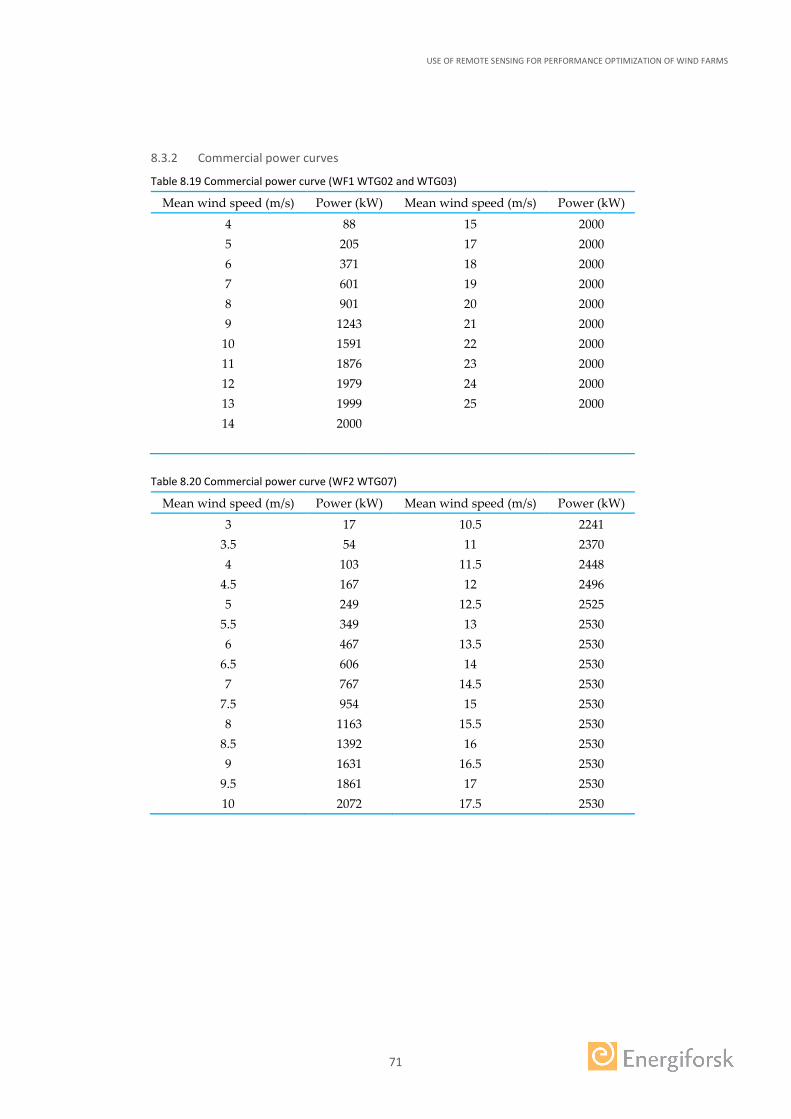
USE OF REMOTE SENSING FOR PERFORMANCE OPTIMIZATION OF WIND FARMS
71
8.3.2 Commercial power curves
Table 8.19 Commercial power curve (WF1 WTG02 and WTG03)
Mean wind speed (m/s) Power (kW) Mean wind speed (m/s) Power (kW)
4 88 15 2000 5 205 17 2000 6 371 18 2000 7 601 19 2000 8 901 20 2000 9 1243 21 2000
10 1591 22 2000 11 1876 23 2000 12 1979 24 2000 13 1999 25 2000 14 2000
Table 8.20 Commercial power curve (WF2 WTG07)
Mean wind speed (m/s) Power (kW) Mean wind speed (m/s) Power (kW)
3 17 10.5 2241 3.5 54 11 2370 4 103 11.5 2448
4.5 167 12 2496 5 249 12.5 2525
5.5 349 13 2530 6 467 13.5 2530
6.5 606 14 2530 7 767 14.5 2530
7.5 954 15 2530 8 1163 15.5 2530
8.5 1392 16 2530 9 1631 16.5 2530
9.5 1861 17 2530 10 2072 17.5 2530
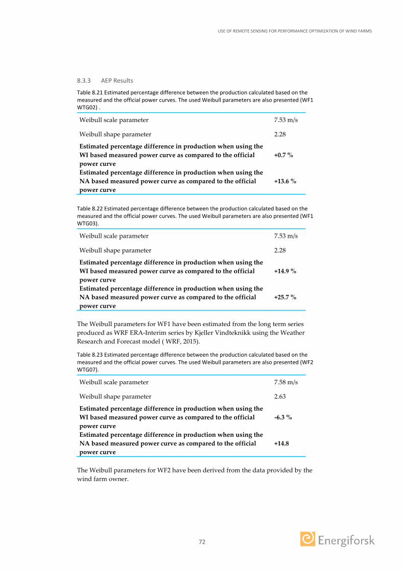
USE OF REMOTE SENSING FOR PERFORMANCE OPTIMIZATION OF WIND FARMS
72
8.3.3 AEP Results
Table 8.21 Estimated percentage difference between the production calculated based on the measured and the official power curves. The used Weibull parameters are also presented (WF1 WTG02) .
Weibull scale parameter 7.53 m/s
Weibull shape parameter 2.28
Estimated percentage difference in production when using the WI based measured power curve as compared to the official power curve
+0.7 %
Estimated percentage difference in production when using the NA based measured power curve as compared to the official power curve
+13.6 %
Table 8.22 Estimated percentage difference between the production calculated based on the measured and the official power curves. The used Weibull parameters are also presented (WF1 WTG03).
Weibull scale parameter 7.53 m/s
Weibull shape parameter 2.28
Estimated percentage difference in production when using the WI based measured power curve as compared to the official power curve
+14.9 %
Estimated percentage difference in production when using the NA based measured power curve as compared to the official power curve
+25.7 %
The Weibull parameters for WF1 have been estimated from the long term series produced as WRF ERA-Interim series by Kjeller Vindteknikk using the Weather Research and Forecast model ( WRF, 2015).
Table 8.23 Estimated percentage difference between the production calculated based on the measured and the official power curves. The used Weibull parameters are also presented (WF2 WTG07).
Weibull scale parameter 7.58 m/s
Weibull shape parameter 2.63
Estimated percentage difference in production when using the WI based measured power curve as compared to the official power curve
-6.3 %
Estimated percentage difference in production when using the NA based measured power curve as compared to the official power curve
+14.8
The Weibull parameters for WF2 have been derived from the data provided by the wind farm owner.

USE OF REMOTE SENSING FOR PERFORMANCE OPTIMIZATION OF WIND FARMS The most recent literature work on underperformance of wind turbines and optimization measures have been summarized.
The main purpose of the project is to gain experience on the use of remote sensing technology in the post construction phase. The turbine performances have been evaluated using a nacelle mounted lidar at four different wind turbines at two Swedish wind farms.
The nacelle mounted lidar has been useful in the evaluation of the turbine yaw alignment relative to the wind direction in short measurement periods. No major yaw errors have been found at the observed wind turbines within this re-search project. There are large discrepancies found between operational power curves and commercial power curves. Moreover, large discrepancies have also been found in comparison of nacelle anemometry measurements with nacelle mounted lidar measurements.
Main challenge for all the measurement campaigns in this research project has been the issues related to the sites terrain complexity, in addition to fact that chosen sites being located at forested and cold climate environments. Relevant topics have been addresses as future work with the use of newly developed re-mote sensing techniques with the investigation of uncertainty sources.
Another step forward in Swedish energy researchEnergiforsk – Swedish Energy Research Centre – an industrially owned body dedicated to me-eting the common energy challenges faced by industries, authorities and society. Our vision is to be hub of Swedish energy research and our mission is to make the world of energy smarter! We are actively meeting current energy challenges by developing new ways to store energy, helping to create a fossil free transportation system, establishing new market models for the heat and power sector, developing new materials and regulating the grid. www.energiforsk.se


![[REMOTE SENSING] 3-PM Remote Sensing](https://img.pdfslide.us/doc/110x75/61f2bbb282fa78206228d9e2/remote-sensing-3-pm-remote-sensing.jpg)


