Use of Regional Climate Model Output for Hydrologic ...sciencepolicy.colorado.edu/admin/publication_files/resource-127-2002.30.pdfb. Regional climate model output The RCM output was

OCTOBER 2002 571H A Y E T A L .

q 2002 American Meteorological Society

Use of Regional Climate Model Output for Hydrologic Simulations

L. E. HAY,* M. P. CLARK,1 R. L. WILBY,# W. J. GUTOWSKI, JR.@ G. H. LEAVESLEY,* Z. PAN,@R. W. ARRITT,@ AND E. S. TAKLE@

*Water Resources Division, U.S. Geological Survey, Denver, Colorado1Cooperative Institute for Research in Environmental Sciences, University of Colorado, Boulder, Colorado

#Department of Geography, King’s College London, Strand, London, United Kingdom@Department of Agronomy, Geological and Atmospheric Sciences, Iowa State University, Ames, Iowa

(Manuscript received 5 October 2001, in final form 1 May 2002)

ABSTRACT

Daily precipitation and maximum and minimum temperature time series from a regional climate model(RegCM2) configured using the continental United States as a domain and run on a 52-km (approximately)spatial resolution were used as input to a distributed hydrologic model for one rainfall-dominated basin (AlapahaRiver at Statenville, Georgia) and three snowmelt-dominated basins (Animas River at Durango, Colorado; eastfork of the Carson River near Gardnerville, Nevada; and Cle Elum River near Roslyn, Washington). For com-parison purposes, spatially averaged daily datasets of precipitation and maximum and minimum temperaturewere developed from measured data for each basin. These datasets included precipitation and temperature datafor all stations (hereafter, All-Sta) located within the area of the RegCM2 output used for each basin, but excludedstation data used to calibrate the hydrologic model.

Both the RegCM2 output and All-Sta data capture the gross aspects of the seasonal cycles of precipitationand temperature. However, in all four basins, the RegCM2- and All-Sta-based simulations of runoff show littleskill on a daily basis [Nash–Sutcliffe (NS) values range from 0.05 to 0.37 for RegCM2 and 20.08 to 0.65 forAll-Sta]. When the precipitation and temperature biases are corrected in the RegCM2 output and All-Sta data(Bias-RegCM2 and Bias-All, respectively) the accuracy of the daily runoff simulations improve dramaticallyfor the snowmelt-dominated basins (NS values range from 0.41 to 0.66 for RegCM2 and 0.60 to 0.76 for All-Sta). In the rainfall-dominated basin, runoff simulations based on the Bias-RegCM2 output show no skill (NSvalue of 0.09) whereas Bias-All simulated runoff improves (NS value improved from 20.08 to 0.72).

These results indicate that measured data at the coarse resolution of the RegCM2 output can be made appropriatefor basin-scale modeling through bias correction (essentially a magnitude correction). However, RegCM2 output,even when bias corrected, does not contain the day-to-day variability present in the All-Sta dataset that isnecessary for basin-scale modeling. Future work is warranted to identify the causes for systematic biases inRegCM2 simulations, develop methods to remove the biases, and improve RegCM2 simulations of daily vari-ability in local climate.

1. Introduction

In recognition of the economic significance of waterresources in the United States, many studies have soughtto examine the effects of climate change on componentsof the hydrologic budget. The most common approachhas been to combine basin-scale hydrologic models withclimate change scenarios derived from general circu-lation model (GCM) output (see Watson et al. 1996).Due to their coarse resolution, GCMs overlook numer-ous climatological details necessary for accurate runoffestimation at the basin scale. The advent of higher-res-olution GCMs may improve the situation; however, hy-drologic modeling at the basin scale requires climato-

Corresponding author address: Dr. L. E. Hay, U.S. GeologicalSurvey, Denver Federal Center, Box 25046, MS 412, Denver, CO80225.E-mail: [email protected]

logical information on scales that are generally farsmaller than the typical grid size of even the highest-resolution GCMs commonly used for climate simula-tions (e.g., Phillips 1995).

In order to translate (‘‘downscale’’) information fromthe coarse-resolution GCMs to the basin scale for hy-drologic modeling, methods are needed that resolve sub-grid-scale information in the simulated fields. One wayto achieve this is by statistical downscaling (Wilks 1995;Wilby et al. 1999). In this approach, empirical relationsare developed between features reliably simulated by aGCM at grid-box scales (e.g., 500-hPa geopotentialheight) and surface predictands at subgrid scales (e.g.,precipitation occurrence and amounts). An alternativeapproach is through dynamical downscaling, in whicha regional climate model (RCM) uses GCM output asinitial and lateral boundary conditions for much morespatially detailed climatological simulations over a re-gion of interest. RCMs capture geographical details

572 VOLUME 3J O U R N A L O F H Y D R O M E T E O R O L O G Y

TABLE 1. Study basins.

Study basin:

Animas Riverat Durango

East fork of the CarsonRiver near Gardnerville

Cle Elum Rivernear Roslyn

Alapaha Riverat Statenville

State Colorado California/Nevada Washington GeorgiaGauging station ID 09361500 10309000 12479000 02317500Drainage area (km2) 1792 922 526 3626Elevation range (m) 2000–3700 1600–3000 680–1800 40–125Number of HRUs 121 96 124 180Number of stations in All-Sta dataset

Precipitation 38 37 27 20Temperature 30 21 14 14

Number of RegCM2 grid points 8 7 5 12Best three-stations sets (Best-Sta)

Precipitation DurangoCascadeLizard Head Pass

Twin LakesHagan’s MeadowLobdell

Fish LakesStampedeStevens Pass

MoultrieFitzgeraldTifton

Temperature DurangoVallecito DamRico

Tahoe ValleyTwin LakesBlue Lakes

BaringCle ElumStampede

QuitmanCordeleAshburn

Snowfall bias (%) 30 0 10 0% days with precipitation (# sta-tions)

71% (15 stations) 23% (1 station) 64% (4 stations) 57% (11 stations)

more precisely than the coarse-resolution GCM. Al-though the computational requirements of such an ap-proach are demanding, rapid advances in computer pow-er over the past decade have allowed RCMs to becomea major tool in climatological studies allowing for lon-ger runs as well as finer resolution.

Wilby et al. (2000) examined the hydrological re-sponse in the Animas River basin of Colorado to dy-namically and statistically downscaled output from theNational Centers for Environmental Prediction–Nation-al Center for Atmospheric Research (NCEP–NCAR) re-analysis (Kalnay et al. 1996). They found that in termsof modeling hydrology, both statistical and dynamicaldownscaling provided greater skill than the coarse-res-olution data used to drive the downscaling. The outputfrom the RCM used in the dynamical downscaling wassimulated by RegCM2 (Giorgi et al. 1996), using thecontinental United States domain and a grid spacing of52 km. Despite the higher level of sophistication andphysical realism associated with dynamical downscal-ing, hydrographs simulated using dynamically down-scaled precipitation and temperature were not generallyas realistic as those simulated using statistically down-scaled precipitation and temperature.

Statistical downscaling (SDS), however, is ultimatelylimited by the assumption of stationarity in the empiricalrelations (i.e., skillful SDS results for the present climatedo not necessarily translate to skillful forecasts of futureclimate). The nonstationarity in empirical climate re-lations is well documented (e.g., Ramage 1983). Dy-namical downscaling does not suffer from such short-comings. Though some parameterization in an RCMmay have an empirical basis, RCM simulations of localclimate are more physically based than SDS and thusare more acceptably transferable from current to future

climates. However, RCM simulations of current climatehave not been extensively tested (Takle et al. 1999).There is a strong need for a systematic assessment ofcurrent RCM output in order to evaluate the skill of(and confidence in) RCM simulations, especially asdrivers for impacts assessment models, and to identifyareas for model improvement. This paper will evaluatean RCM-surface climate, by using the RegCM2 (Giorgiet al. 1996) simulated precipitation and temperature asinput to a hydrologic model.

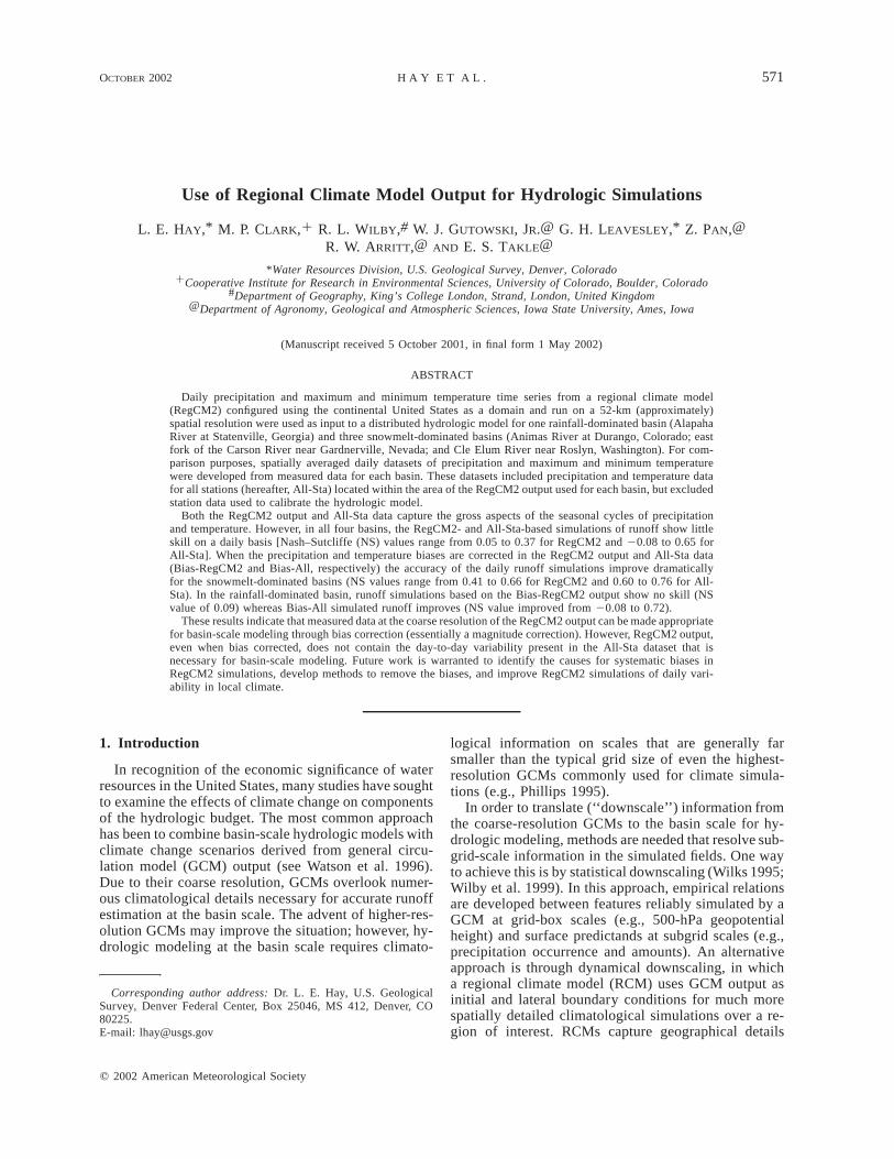
Four basins were chosen for this analysis: 1) AnimasRiver at Durango, Colorado (Animas); 2) east fork ofthe Carson River near Gardnerville, Nevada (Carson);3) Cle Elum River near Roslyn, Washington (Cle Elum);and 4) Alapaha River at Statenville, Georgia (Alapaha).The surface hydrology of the first three basins (Animas,Carson, and Cle Elum) is dominated by snowmelt. TheCarson and Cle Elum basins are also characterized byfrequent rain-on-snow events in the winter months. TheAlapaha basin is a low-elevation rainfall-dominated ba-sin. Tables 1 and 2 list some of the defining features ofeach basin, and Fig. 1 shows the location of each. Inthis study, for each of the four basins, daily precipitationand temperature were derived from RegCM2 and usedas inputs to a hydrologic model. Since the hydrologicalresponse of the basin is an integration of the regionalclimate (in time and space), the results presented herewill provide insights into the overall realism of theRegCM2 precipitation and temperature time series forfour basins in the United States. This study examinesthe limits of what one can do with RegCM2 output thathas been configured using the continental United Statesas a domain and run on a 52-km (approximately) spatialresolution, and what the implications are for a RegCM2to be able to handle details of climate at those limits.


TABLE 2. Elevation ranges.

Elevations ranges (m) for each study basin

Animas River at Durango

Min Mean Max

East fork of the CarsonRiver near Gardnerville

Min Mean Max

Cle Elum River nearRoslyn

Min Mean Max

Alapaha River atStatenville

Min Mean Max

HRUs 2011 3060 3728 1645 2300 2959 680 1337 1799 44 85 122Best three-stations

PrecipitationTemperature

20102010

26092341

31092682

24381906

25602260

28042438

1027235

1162678

12411219

316172

338287

353404

All stationsPrecipitationTemperature

17201720

26862328

35363536

718718

19091104

28042804

5252

813328

18291640

112112

227197

455455

RegCM2 grid nodes 1895 2579 2987 1586 1926 2166 279 802 1401 23 64 139

FIG. 1. Location of study basins.

2. Data

For each basin, two types of daily data were compiledfor the purpose of hydrologic modeling: 1) measured-station data and 2) RegCM2 output.

a. Station data

Daily maximum and minimum temperatures and pre-cipitation data from stations in and around each basin werecompiled from the National Weather Service (NWS) andsnow telemetry (SNOTEL) databases. The NWS data wereretrieved from the Utah Climate Center’s Weather DataOnline (available online at http://climate.usu.edu/Free/).SNOTEL data were retrieved from the Natural ResourcesConservation Service (available online at ftp://162.79.124.23/data/snow/snotel/snothist/). Figure 2 showsthe location of the NWS and SNOTEL stations used foreach basin study.

b. Regional climate model output

The RCM output was simulated by RegCM2 (Giorgiet al. 1996), using the continental U.S. domain of theProject to Intercompare Regional Climate Simulations(PIRCS) experiments (see Fig. 1 in Takle et al. 1999).Precipitation was simulated using the Grell (1993) con-vection scheme and the simple warm-cloud explicitmoisture scheme of Hsie et al. (1984). The simulationsalso used the CCM2 radiation package (Briegleb 1992),the BATS version 1e surface package (Dickinson et al.1992), and the nonlocal boundary layer turbulencescheme of Holtslag et al. (1990).

A 10-yr run (1979–88) was conducted using 6-h out-put from the NCEP–NCAR reanalysis to define initialand boundary conditions. These were supplemented byobservations of water-surface temperature in the Gulfof California and the Great Lakes, which are poorlyresolved in the reanalysis.


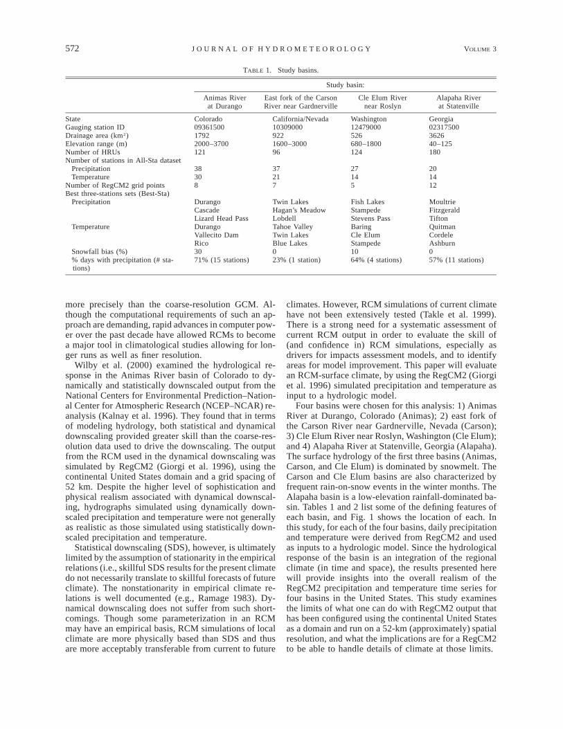
FIG. 2. Station locations and RegCM2 grid points used in each basin.

The RegCM2 grid spacing is 52 km on a Lambertconformal projection of the midlatitudes. Figure 2shows the RegCM2 grid points chosen for analysis ineach of the four study basins. A buffer equal to that ofthe RegCM2 grid spacing was generated around eachbasin boundary, and all RegCM2 grid points that fellwithin this buffered area were chosen for this analysis(see Fig. 2). This provided 8 grid points for the Animas,5 grid points for the Cle Elum, 7 grid points for theCarson, and 12 grid points for the Alapaha (Table 1).The area of a RegCM2 grid box is approximately 2500km2, larger than the drainage area of three of the fourbasins (Table 1). The four basins are comparable in sizeto the smallest scales resolved by the RegCM2. Thus,they represent a fairly stringent test of the limits of themodel’s downscaling capability.

3. Hydrologic model

The hydrologic model chosen for this study is theU.S. Geological Survey’s (USGS) Precipitation RunoffModeling System (PRMS) (Leavesley et al. 1983; Leav-esley and Stannard 1995). PRMS is a distributed-pa-

rameter, physically based watershed model. Distributedparameter capabilities are provided by partitioning a wa-tershed into hydrologic response units (HRUs). Basinand HRU delineation, characterization, and parameter-ization were done for each basin using a geographicinformation system (GIS) interface. HRUs were delin-eated identically for each basin by 1) subdividing thebasin into two flow planes for each channel, 2) subdi-viding the basin using three equal area elevation bands,and 3) intersecting the flow-plane map with the eleva-tion-band map. The number of HRUs resulting fromthis process for each basin are listed in Table 1. Theelevation ranges of the HRUs are listed in Table 2.

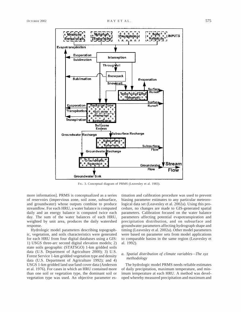
A conceptual diagram of PRMS is shown in Fig. 3(Leavesley et al. 1983). PRMS uses daily inputs of theclimate variables precipitation, maximum temperature,minimum temperature, and solar radiation. Precipita-tion, maximum temperature, and minimum temperatureare available at most climate stations across the UnitedStates. Solar radiation is generally not measured at theclimate stations used in this study, so shortwave andlongwave radiation were computed empirically usingalgorithms in PRMS [see Leavesley et al. (1983) for


FIG. 3. Conceptual diagram of PRMS (Leavesley et al. 1983).

more information]. PRMS is conceptualized as a seriesof reservoirs (impervious zone, soil zone, subsurface,and groundwater) whose outputs combine to producestreamflow. For each HRU, a water balance is computeddaily and an energy balance is computed twice eachday. The sum of the water balances of each HRU,weighted by unit area, produces the daily watershedresponse.

Hydrologic model parameters describing topograph-ic, vegetation, and soils characteristics were generatedfor each HRU from four digital databases using a GIS:1) USGS three-arc second digital elevation models; 2)state soils geographic (STATSGO) 1-km gridded soilsdata (U.S. Department of Agriculture 2000); 3) U.S.Forest Service 1-km gridded vegetation type and densitydata (U.S. Department of Agriculture 1992); and 4)USGS 1-km gridded land use/land cover data (Andersonet al. 1976). For cases in which an HRU contained morethan one soil or vegetation type, the dominant soil orvegetation type was used. An objective parameter es-

timation and calibration procedure was used to preventbiasing parameter estimates to any particular meteoro-logical data set (Leavesley et al. 2002a). Using this pro-cedure, no changes are made to GIS-generated spatialparameters. Calibration focused on the water balanceparameters affecting potential evapotranspiration andprecipitation distribution, and on subsurface andgroundwater parameters affecting hydrograph shape andtiming (Leavesley et al. 2002a). Other model parameterswere based on parameter sets from model applicationsto comparable basins in the same region (Leavesley etal. 1992).

a. Spatial distribution of climate variables—The xyzmethodology

The hydrologic model PRMS needs reliable estimatesof daily precipitation, maximum temperature, and min-imum temperature at each HRU. A method was devel-oped whereby measured precipitation and maximum and


minimum temperature data from a group of stations (orRegCM2 grid points) could be spatially distributed fromone point (a single daily mean value) to each HRU ina basin (Hay et al. 2000; Hay and Clark 2000). Themethod allows for station data and RegCM2 grid pointsto be distributed similarly, both starting as a single dailymean value.

Significant geographic factors affecting the spatialdistribution of precipitation, maximum temperature, andminimum temperature distributions within a river basinare latitude (x), longitude (y), and elevation (z). To ac-count for seasonal climate variations, the multiple linearregression (MLR) equation (Eq. 1) was developed foreach basin and month for each dependent variable [theclimate variables (CVs): precipitation, maximum andminimum temperature) using the independent variablesof x, y, and z from a set of climate stations that fellwithin the buffered areas designated in Fig. 2:

CV 5 b x 1 b y 1 b z 1 b .1 2 3 0 (1)

The monthly MLR equations were computed to de-termine the regression surface that described the spatialrelations between the monthly dependent CV and theindependent xyz variables. Equation (1) describes aplane in three-dimensional space with ‘‘slopes’’ b1, b2,and b3 intersecting the CV axis at b0. Note that for eachmonth the best MLR equation did not always includeall the independent variables.

To estimate the daily CVs for each HRU, the follow-ing procedure was followed: 1) mean daily CVs andcorresponding mean x, y, and z values from a set ofstations or grid points were used with the slopes of themonthly MLRs in Eq. (1) to estimate a unique y intercept( ) for that day, and 2) equation 2 was then solvedestb 0

using b1, b2, and b3 from Eq. (1) and the x, y, and zvalues of the HRUs:

estCV 5 b 1 b x 1 b y 1 b z . (2)(HRU) 0 1 (HRU) 2 (HRU) 3 (HRU)

The distribution technique is identical for station andRegCM2 grid-node output: the same MLR equationsare used but the time series of mean daily CVs and theircorresponding mean x, y, and z values are obtained fromeither station data or from the RegCM2 grid points toestimate a unique for that day. Thus, for a givenestb 0

day the slope of the MLRs for the CVs remained con-stant, but the y intercept changes based on the mean CVand xyz values.

b. Exhaustive search analysis

The MLR-distribution methodology provides spatial‘‘maps’’ of precipitation and temperature based on re-gional relations between latitude, longitude and eleva-tion, and local climate. However, these MLR equationsdo not provide a perfect fit with observations; the re-gional MLR equations often under estimate or overes-timate the mean precipitation (or temperature) in thesmaller basins used for hydrologic simulations. Also,

difficulties in precipitation measurement (particularlyprecipitation gage undercatch associated with snowfallevents) may lead to significant errors in hydrologic sim-ulations.

To address these issues, an exhaustive search (ES)analysis was used to 1) determine the ‘‘optimal’’ pre-cipitation- and temperature-station sets to anchor the xyzdistribution methodology (Hay et al. 2000; Wilby et al.1999); 2) provide an estimate of snowfall-measurementbias associated with the above precipitation-station set(Hay et al. 2000); and 3) define a separate precipitation-station set to determine daily precipitation frequency.The ES analysis was executed using water years 1989–96. Climate stations were tested in the ES analysis ifthey had less than 5% missing record for water years1989–96 and the period of the RegCM2 data (1979–88). This excluded many of the SNOTEL stations whoserecords did not begin until the mid 1980s.

To start the ES search, each climate station was testedindividually for its ability to anchor the xyz methodol-ogy. Precipitation and temperature stations were testedseparately since the best precipitation station choicegenerally differed from the best choice for temperaturedistribution in a basin. For every combination of theseprecipitation and temperature xyz-station sets, a snowfallbias error (described below) and a station set to indicateprecipitation frequency (described below) were tested.Time series of precipitation, maximum temperature, andminimum temperature for each of these combinationswere calculated and used as input into PRMS. Measuredand simulated runoff were compared by examining thesum of the daily absolute errors between the two.

Previous work using this method of station selectionin the Animas River basin (Wilby et al. 2000) high-lighted the problem of gauge undercatch, estimated tobe as much as 20–50% for snowfall in mountainousterrain (Sevruk 1989). Milly and Dunne (2002) foundthat a 10%–20% bias in precipitation was typical forbasins examined around the world. An attempt to correctfor these biases in snowfall was made by testing un-dercatch amounts from 0%–50% during snowfall eventsfor each station combination tested in the ES analysis.This bias correction in the ES analysis actually com-pensates for the net effect of a number of biases relatedto precipitation measurement, such as gauge undercatch,gauge location, and/or lack of gauges at high elevation.It may also correct for other problems in PRMS, suchas overestimation of ET.

Precipitation frequency was incorporated into PRMSbased on a set of precipitation stations separate fromthe set selected for use in the xyz methodology. Prelim-inary work with the precipitation-station set chosen toanchor the xyz methodology indicated that the optimalxyz-station set used to produce the volume of precipi-tation for a day was not always the best set to determinewhether there actually was precipitation on that day.Therefore, for each ES search, a separate precipitation-station set was used to indicate a rain or no-rain day


TABLE 3. Meteorological inputs to the hydrology model.

No. Abbreviation Description

1 Best-Sta Best three-station set determined throughES analysis

2 RegCM2 RegCM2 grid nodes within buffered area3 All-Sta All stations within buffered area excluding

‘‘Best-Sta’’ stations4 Bias-RegCM2 ‘‘RegCM2’’ with a Bias correction applied5 Bias-All ‘‘All-Sta’’ stations with a Bias correction

applied6 Test1 ‘‘Best-Sta’’ precipitation, ‘‘Bias-RegCM2’’

max and min temperature7 Test2 ‘‘Best-Sta’’ max temperature, ‘‘Bias-

RegCM2’’ min temperature and precipi-tation

8 Test3 ‘‘Best-Sta’’ min temperature, ‘‘Bias-RegCM2’’ max temperature and precipi-tation

(i.e., if any of the stations in the chosen set had pre-cipitation, then the xyz methodology was enacted to dis-tribute precipitation on that day).

Further ES searches using the above procedure wererun to test all possible combinations of two, three, andfour station groups comprising the xyz-station sets. Foreach ES search, the best xyz-station set for temperatureand precipitation with an associated snowfall bias and pre-cipitation frequency was determined by comparing the ab-solute error in runoff. The ES analysis ended when theabsolute error associated with the above combinationshowed no significant improvement from one group to thenext. Table 1 lists the ‘‘best’’ temperature and precipitationstation sets and Fig. 2 shows their locations. In addition,Table 1 lists the snowfall bias associated with the precip-itation-station set and percentage of days with precipitationand associated number of stations used to designate theprecipitation frequency for each basin.

This ES procedure avoids the need for an exhaustivecalibration of hydrologic model parameters. Model cali-bration is used quite often in hydrologic modeling to avoidthe reality of serious biases in precipitation (Milly andDunne 2002). The ES procedure is similar to many of themodel calibration procedures that are in widespread useand will indirectly compensate for problems in other rou-tines in the hydrologic model. However, the problems withprecipitation bias are corrected at their source, thus re-ducing the need to directly calibrate any of the GIS-gen-erated spatial parameters. In this study these estimates ofspatial parameters were not calibrated to avoid biasingthem to any specific meteorological time series.

c. Input datasets

The input datasets for the hydrologic model are de-rived from two sources: 1) RegCM2 output and 2) mea-sured-station data. In order to assess the performanceof the RegCM2-based simulations of runoff it becamenecessary to develop an appropriate baseline. Our hy-drologic modeling strategy consists of selecting the sta-tion set that provides the best simulation of runoff (Best-Sta from the ES analysis), and then tune a small selectgroup of model parameters to provide the best possiblesimulation of runoff given the chosen station set timeseries (Leavesley et al. 2002b). No such calibration isperformed on the RegCM2 model inputs. Thus, use ofthe calibrated Best-Sta mean time series to assessRegCM2 performance will lead to conclusions that arefavorable to the station-based simulations and unfavor-able to RegCM2-based runoff simulations.

To provide a fair means of comparing the relative per-formance of RegCM2- and station-based runoff simu-lations, new input datasets consisting of regionally av-eraged station measurements were developed. These da-tasets (hereafter referred to as ‘‘All-Sta’’) include dataon precipitation and temperature for all stations that fellwithin the RegCM2 buffers (Fig. 2), but excludes thestation set (Best-Sta) determined using the ES procedure

and used for model calibration. The Best-Sta set is onlyused in this study to provide the best possible set of modelparameters, and this parameter set is used for both theRegCM2- and All-Sta simulations. The ES analysis isused to determine the Best-Sta datasets but is not usedin the RegCM2 or All-Sta datasets. RegCM2 and All-Sta simulations are corrected for systematic bias (Bias-RegCM2 and Bias-All, respectively) to distinguish errorsin hydrologic simulations associated with model biasesfrom errors in hydrologic simulations associated withmodel problems in capturing daily climate variations. Allinput datasets are summarized in Table 3.

4. Hydrologic model input data

The hydrologic model PRMS was forced with me-teorological variables derived from two sources: 1)RegCM2 output and 2) measured-station data. RegCM2output for the United States was available from 1979to 1988. In each basin, PRMS was initialized with sta-tion data from 1 October 1977 to 31 December 1978 toremove the bias from the state variables. Then, 10 years(1979–88) of daily mean precipitation, maximum tem-perature, and minimum temperature from climate sta-tions and RegCM2 output (outlined in Table 3) weredistributed using the xyz methodology to the HRUs ineach basin to produce daily runoff.

a. Precipitation

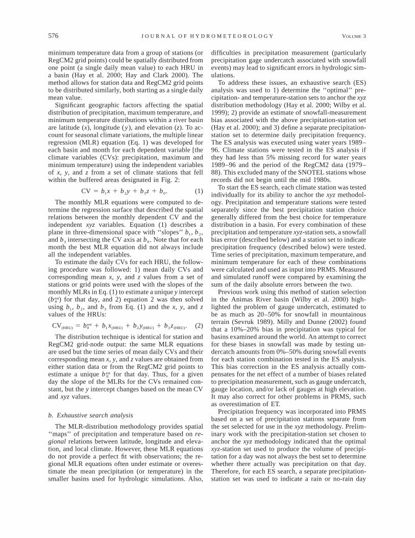
The RegCM2 output has a significantly higher num-ber of precipitation days than measured at individualstations. Such differences occur partly because theRegCM2 precipitation represents an area (grid cells ap-proximately 52 km 3 52 km) not a point. To evaluatethese differences directly, Fig. 4 compares the percent-age of precipitation days between the All-Sta data andthe RegCM2 output (see Table 3 for dataset description)over successively larger areas, starting from the centerof each basin. In Fig. 4, each square (circle) represents


FIG. 4. Percent precipitation days with increasing buffer size for station data and RegCM2output.

the inclusion of an additional station (RegCM2 gridpoint). The triangle in each plot indicates the percentprecipitation days associated with the Best-Sta dataset(plotted vs basin area). As expected, increases in area(and the number of stations) are accompanied by in-creases in the percentage of precipitation days. However,notice that in each basin the RegCM2 starts with a sig-nificantly higher number of precipitation days at thesmallest area (Fig. 4). Part of these differences occurbecause even a trace of RegCM2-generated precipitationwill show up as a precipitation day (vs the 0.01-inchdetection limit from the stations). When the station de-tection limit of 0.01 inches is applied as a cutoff to theRegCM2 output (open ovals in Fig. 4), there is closeconcurrence with the station data (with the exception of

the Alapaha River basin); but due to the large area rep-resented by a single RegCM2 grid box, there is still ahigher percentage of precipitation days than what wasdetermined from the exhaustive search analysis (Table1 and triangle in Fig. 4).

Figures 5a–8a show the daily basin precipitationmean by month for the Best-Sta, RegCM2, Bias-RegCM2 (described later), All-Sta, and Bias-All (de-scribed later) datasets for the four river basins. Com-parison of the RegCM2 and All-Sta with the Best-Staprecipitation dataset shows that both the RegCM2 andAll-Sta capture the gross aspects of the seasonal cycleof precipitation in all four basins, although there aresome large discrepancies. In the Alapaha River basin(Fig. 5a), RegCM2 values are significantly lower than


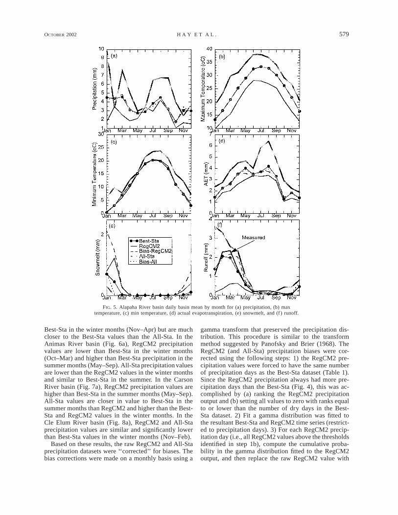
FIG. 5. Alapaha River basin daily basin mean by month for (a) precipitation, (b) maxtemperature, (c) min temperature, (d) actual evapotranspiration, (e) snowmelt, and (f ) runoff.

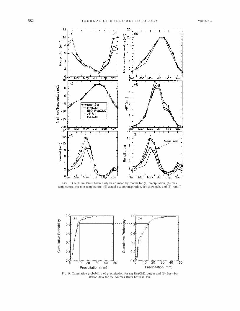
Best-Sta in the winter months (Nov–Apr) but are muchcloser to the Best-Sta values than the All-Sta. In theAnimas River basin (Fig. 6a), RegCM2 precipitationvalues are lower than Best-Sta in the winter months(Oct–Mar) and higher than Best-Sta precipitation in thesummer months (May–Sep). All-Sta precipitation valuesare lower than the RegCM2 values in the winter monthsand similar to Best-Sta in the summer. In the CarsonRiver basin (Fig. 7a), RegCM2 precipitation values arehigher than Best-Sta in the summer months (May–Sep).All-Sta values are closer in value to Best-Sta in thesummer months than RegCM2 and higher than the Best-Sta and RegCM2 values in the winter months. In theCle Elum River basin (Fig. 8a), RegCM2 and All-Staprecipitation values are similar and significantly lowerthan Best-Sta values in the winter months (Nov–Feb).

Based on these results, the raw RegCM2 and All-Staprecipitation datasets were ‘‘corrected’’ for biases. Thebias corrections were made on a monthly basis using a

gamma transform that preserved the precipitation dis-tribution. This procedure is similar to the transformmethod suggested by Panofsky and Brier (1968). TheRegCM2 (and All-Sta) precipitation biases were cor-rected using the following steps: 1) the RegCM2 pre-cipitation values were forced to have the same numberof precipitation days as the Best-Sta dataset (Table 1).Since the RegCM2 precipitation always had more pre-cipitation days than the Best-Sta (Fig. 4), this was ac-complished by (a) ranking the RegCM2 precipitationoutput and (b) setting all values to zero with ranks equalto or lower than the number of dry days in the Best-Sta dataset. 2) Fit a gamma distribution was fitted tothe resultant Best-Sta and RegCM2 time series (restrict-ed to precipitation days). 3) For each RegCM2 precip-itation day (i.e., all RegCM2 values above the thresholdsidentified in step 1b), compute the cumulative proba-bility in the gamma distribution fitted to the RegCM2output, and then replace the raw RegCM2 value with


FIG. 6. Animas River basin daily basin mean by month for (a) precipitation, (b) maxtemperature, (c) min temperature, (d) actual evapotranspiration, (e) snowmelt, and (f ) runoff.

the precipitation amount associated with the matchedcumulative probability in the gamma distribution fittedto the Best-Sta data. An example of this approach isgiven in Fig. 9, which shows the cumulative probabilityof precipitation for RegCM2 output (Fig. 9a) and Best-Sta data (Fig. 9b) for the Animas River basin in January.Note from Fig. 6 that the RegCM2 model underpredictscold-season precipitation in the Animas. For a RegCM2precipitation value of 10 mm, the cumulative probabilityin the fitted gamma distribution is 0.83. In the gammafit to the measured data, a cumulative probability of 0.83is associated with a precipitation value of 15 mm. Forthis particular case, the bias correction increases theRegCM2 prediction from 10 to 15 mm.

Precipitation-day frequency is corrected using a meth-od identical to step 1, except the station set used is theBest-Sta set determined from the exhaustive search anal-ysis for precipitation frequency. Because there wereonly 10 years of RegCM2 output available for this study,

an independent dataset was not used to produce theRegCM2 precipitation bias corrections. From Figs. 5a–8a, it is evident that monthly values of Bias-RegCM2and Bias-All are similar to Best-Sta data.

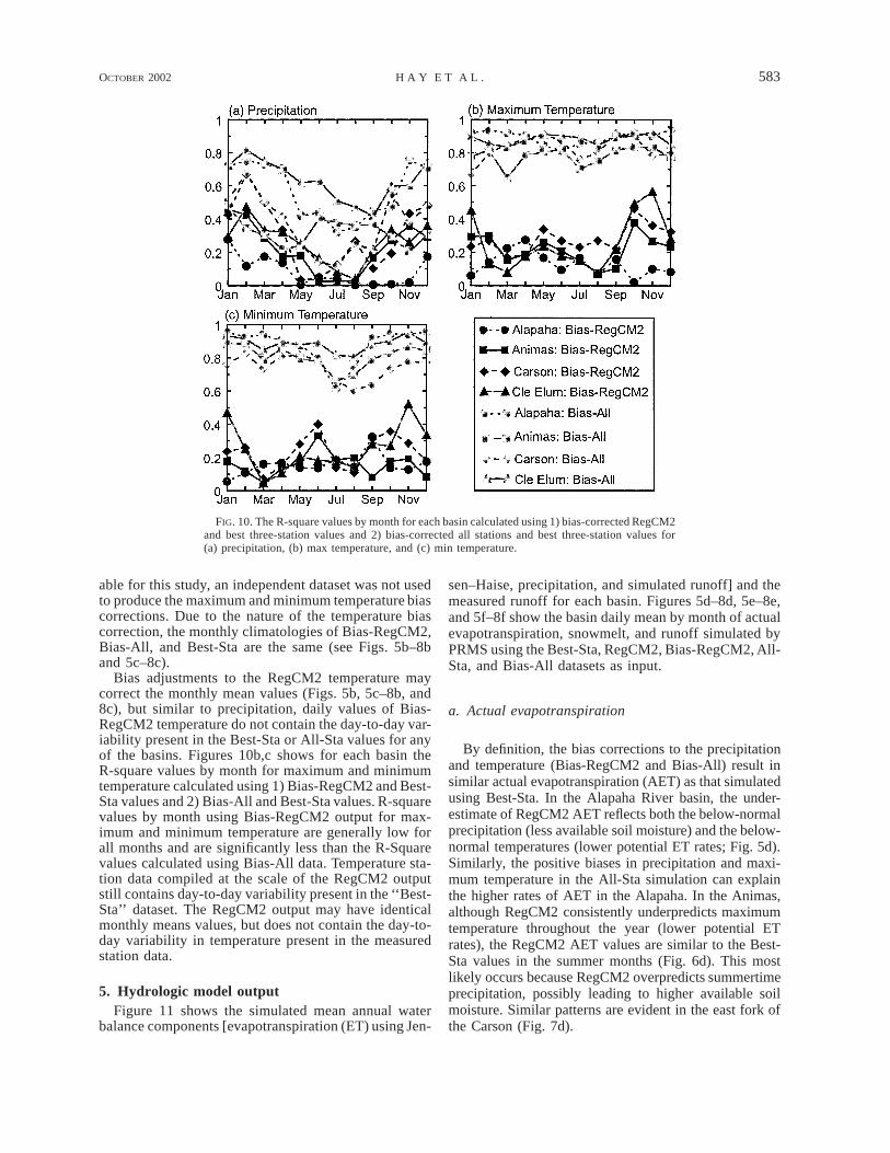
The bias adjustments to the RegCM2 precipitationmay correct the monthly mean values (Figs. 5f–8f), butdaily values of Bias-RegCM2 precipitation do not con-tain the day-to-day variability present in the Best-Sta orAll-Sta values for any of the basins. Figure 10a showsfor each basin the R-square values by month for pre-cipitation calculated using 1) Bias-RegCM2 and Best-Sta values and 2) Bias-All and Best-Sta values. The R-square values using Bias-RegCM2 precipitation output(Fig. 10a) are generally low for most months, especiallyin the Alapaha River basin (remaining near 0.0 for a largeportion of the year). Relatively higher values occur inthe winter months and the lowest values occur in thesummer months. The R-square values using Bias-All pre-cipitation output are much higher than those from Bias-


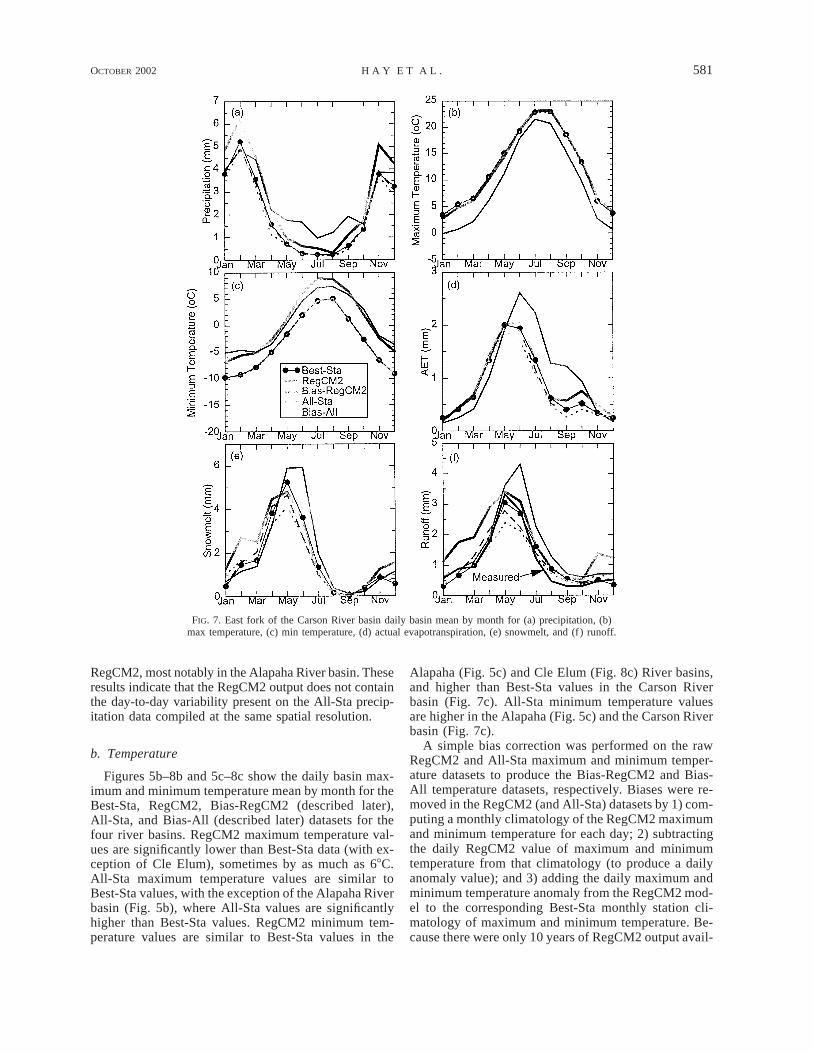
FIG. 7. East fork of the Carson River basin daily basin mean by month for (a) precipitation, (b)max temperature, (c) min temperature, (d) actual evapotranspiration, (e) snowmelt, and (f) runoff.

RegCM2, most notably in the Alapaha River basin. Theseresults indicate that the RegCM2 output does not containthe day-to-day variability present on the All-Sta precip-itation data compiled at the same spatial resolution.

b. Temperature

Figures 5b–8b and 5c–8c show the daily basin max-imum and minimum temperature mean by month for theBest-Sta, RegCM2, Bias-RegCM2 (described later),All-Sta, and Bias-All (described later) datasets for thefour river basins. RegCM2 maximum temperature val-ues are significantly lower than Best-Sta data (with ex-ception of Cle Elum), sometimes by as much as 68C.All-Sta maximum temperature values are similar toBest-Sta values, with the exception of the Alapaha Riverbasin (Fig. 5b), where All-Sta values are significantlyhigher than Best-Sta values. RegCM2 minimum tem-perature values are similar to Best-Sta values in the

Alapaha (Fig. 5c) and Cle Elum (Fig. 8c) River basins,and higher than Best-Sta values in the Carson Riverbasin (Fig. 7c). All-Sta minimum temperature valuesare higher in the Alapaha (Fig. 5c) and the Carson Riverbasin (Fig. 7c).

A simple bias correction was performed on the rawRegCM2 and All-Sta maximum and minimum temper-ature datasets to produce the Bias-RegCM2 and Bias-All temperature datasets, respectively. Biases were re-moved in the RegCM2 (and All-Sta) datasets by 1) com-puting a monthly climatology of the RegCM2 maximumand minimum temperature for each day; 2) subtractingthe daily RegCM2 value of maximum and minimumtemperature from that climatology (to produce a dailyanomaly value); and 3) adding the daily maximum andminimum temperature anomaly from the RegCM2 mod-el to the corresponding Best-Sta monthly station cli-matology of maximum and minimum temperature. Be-cause there were only 10 years of RegCM2 output avail-


FIG. 8. Cle Elum River basin daily basin mean by month for (a) precipitation, (b) maxtemperature, (c) min temperature, (d) actual evapotranspiration, (e) snowmelt, and (f ) runoff.

FIG. 9. Cumulative probability of precipitation for (a) RegCM2 output and (b) Best-Stastation data for the Animas River basin in Jan.


FIG. 10. The R-square values by month for each basin calculated using 1) bias-corrected RegCM2and best three-station values and 2) bias-corrected all stations and best three-station values for(a) precipitation, (b) max temperature, and (c) min temperature.

able for this study, an independent dataset was not usedto produce the maximum and minimum temperature biascorrections. Due to the nature of the temperature biascorrection, the monthly climatologies of Bias-RegCM2,Bias-All, and Best-Sta are the same (see Figs. 5b–8band 5c–8c).

Bias adjustments to the RegCM2 temperature maycorrect the monthly mean values (Figs. 5b, 5c–8b, and8c), but similar to precipitation, daily values of Bias-RegCM2 temperature do not contain the day-to-day var-iability present in the Best-Sta or All-Sta values for anyof the basins. Figures 10b,c shows for each basin theR-square values by month for maximum and minimumtemperature calculated using 1) Bias-RegCM2 and Best-Sta values and 2) Bias-All and Best-Sta values. R-squarevalues by month using Bias-RegCM2 output for max-imum and minimum temperature are generally low forall months and are significantly less than the R-Squarevalues calculated using Bias-All data. Temperature sta-tion data compiled at the scale of the RegCM2 outputstill contains day-to-day variability present in the ‘‘Best-Sta’’ dataset. The RegCM2 output may have identicalmonthly means values, but does not contain the day-to-day variability in temperature present in the measuredstation data.

5. Hydrologic model outputFigure 11 shows the simulated mean annual water

balance components [evapotranspiration (ET) using Jen-

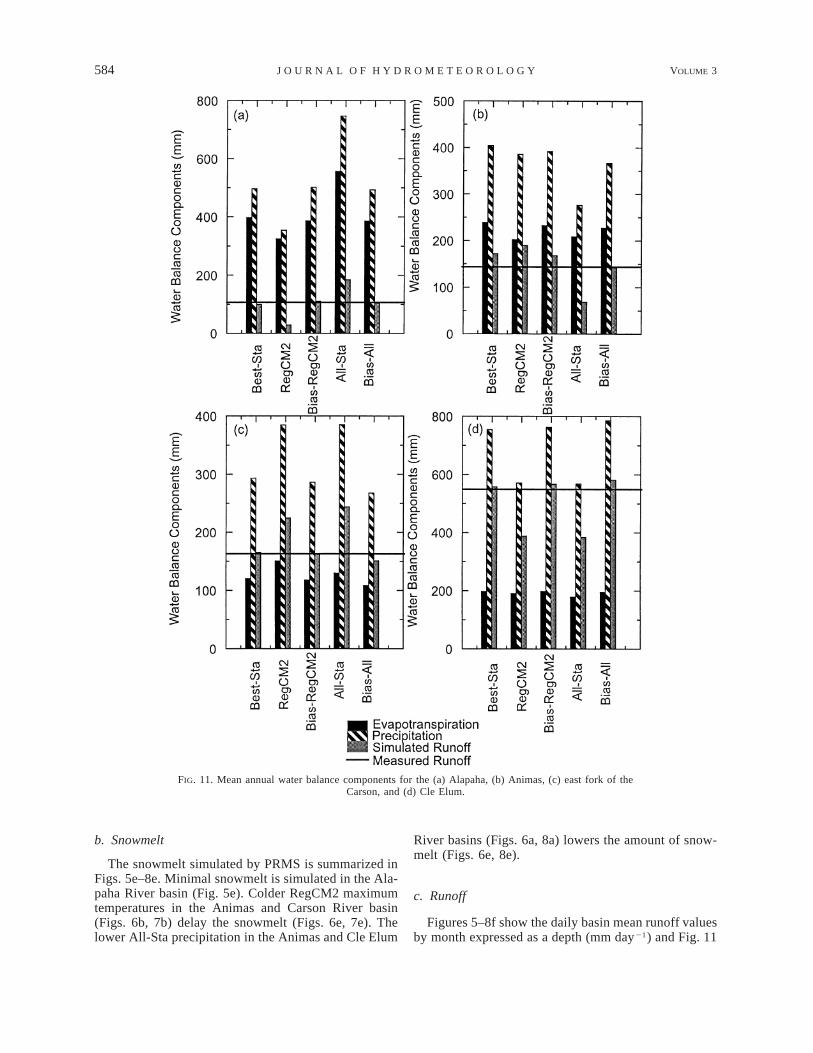
sen–Haise, precipitation, and simulated runoff] and themeasured runoff for each basin. Figures 5d–8d, 5e–8e,and 5f–8f show the basin daily mean by month of actualevapotranspiration, snowmelt, and runoff simulated byPRMS using the Best-Sta, RegCM2, Bias-RegCM2, All-Sta, and Bias-All datasets as input.

a. Actual evapotranspiration

By definition, the bias corrections to the precipitationand temperature (Bias-RegCM2 and Bias-All) result insimilar actual evapotranspiration (AET) as that simulatedusing Best-Sta. In the Alapaha River basin, the under-estimate of RegCM2 AET reflects both the below-normalprecipitation (less available soil moisture) and the below-normal temperatures (lower potential ET rates; Fig. 5d).Similarly, the positive biases in precipitation and maxi-mum temperature in the All-Sta simulation can explainthe higher rates of AET in the Alapaha. In the Animas,although RegCM2 consistently underpredicts maximumtemperature throughout the year (lower potential ETrates), the RegCM2 AET values are similar to the Best-Sta values in the summer months (Fig. 6d). This mostlikely occurs because RegCM2 overpredicts summertimeprecipitation, possibly leading to higher available soilmoisture. Similar patterns are evident in the east fork ofthe Carson (Fig. 7d).


FIG. 11. Mean annual water balance components for the (a) Alapaha, (b) Animas, (c) east fork of theCarson, and (d) Cle Elum.

b. Snowmelt

The snowmelt simulated by PRMS is summarized inFigs. 5e–8e. Minimal snowmelt is simulated in the Ala-paha River basin (Fig. 5e). Colder RegCM2 maximumtemperatures in the Animas and Carson River basin(Figs. 6b, 7b) delay the snowmelt (Figs. 6e, 7e). Thelower All-Sta precipitation in the Animas and Cle Elum

River basins (Figs. 6a, 8a) lowers the amount of snow-melt (Figs. 6e, 8e).

c. Runoff

Figures 5–8f show the daily basin mean runoff valuesby month expressed as a depth (mm day21) and Fig. 11


shows the mean annual water balance components foreach basin. In the Alapaha, the more frequent but small-er-magnitude storms generated by the RegCM2 have amean monthly depth that is about 80% of the measuredmean monthly (Fig. 5a). The significant smaller averagemonthly runoff simulated using the RegCM2 storms(Fig. 5f) can be attributed to the smaller magnitude ofthe individual storms present in the RegCM2 output.Figure 4d indicates a 90% rainday occurrence in theRegCM2 output, compared with 58 and 62 percent rain-day occurrence in the Best-Sta and All-Sta datasets,respectively. For direct-runoff computation at a 24-htime step, the PRMS model uses a contributing areaconcept similar to that used by many watershed models.The area contributing runoff during rainfall, and themagnitude of the runoff from this area are functions ofantecedent soil moisture content and the 24-h rainfallamount. This relation is nonlinear with larger stormsand wetter soil conditions generating proportionallylarger amounts of runoff than that from drier soil con-ditions and smaller storms. Thus, precipitation fromlarger storms will reach river networks fairly quickly,whereas precipitation from smaller storms will replenishsoil reservoirs and remain available for ET. Note thatalmost all of the precipitation in the raw RegCM2 sim-ulation is lost through ET (Fig. 11a), resulting in verylow runoff (Fig. 5f). The less frequent but larger-mag-nitude storms in the Best-Sta data produce a simulatedrunoff response that is much closer to the measuredbasin runoff (Fig. 5f). The larger precipitation volumesfor the All-Sta produced excessively high runoff values.

In the Animas (Fig. 6), significantly lower RegCM2maximum temperature values translates into delays inspring runoff. Similar delays in spring runoff from lowerRegCM2 maximum temperature are seen in each of thesnowmelt basins (Figs. 6–8f). Lower All-Sta precipi-tation in the Animas results in underestimation of runoff.Similar but less extreme runoff responses are seen inthe Cle Elum (Fig. 8). In the east fork of the Carson(Fig. 7), higher All-Sta and RegCM2 precipitation val-ues translate into an overestimation of runoff.

6. Diagnosis of hydrologic modeling error

PRMS-simulated runoff using RegCM2 and All-Stainput datasets did not reproduce realistic hydrographsin any of the basins. Runoff simulated using the Bias-corrected RegCM2 and All-Sta datasets are much closerto measured mean monthly runoff than those simulatedusing the raw data. But, comparisons of runoff valueson a mean monthly basis can be misleading. As shownin Fig. 10, the bias correction, essentially a magnitudecorrection to the raw climate datasets, does not correctfor errors in daily temporal variability. A comparisonof daily runoff is a more stringent test of the capabilitiesof RegCM2 to simulate observed climate.

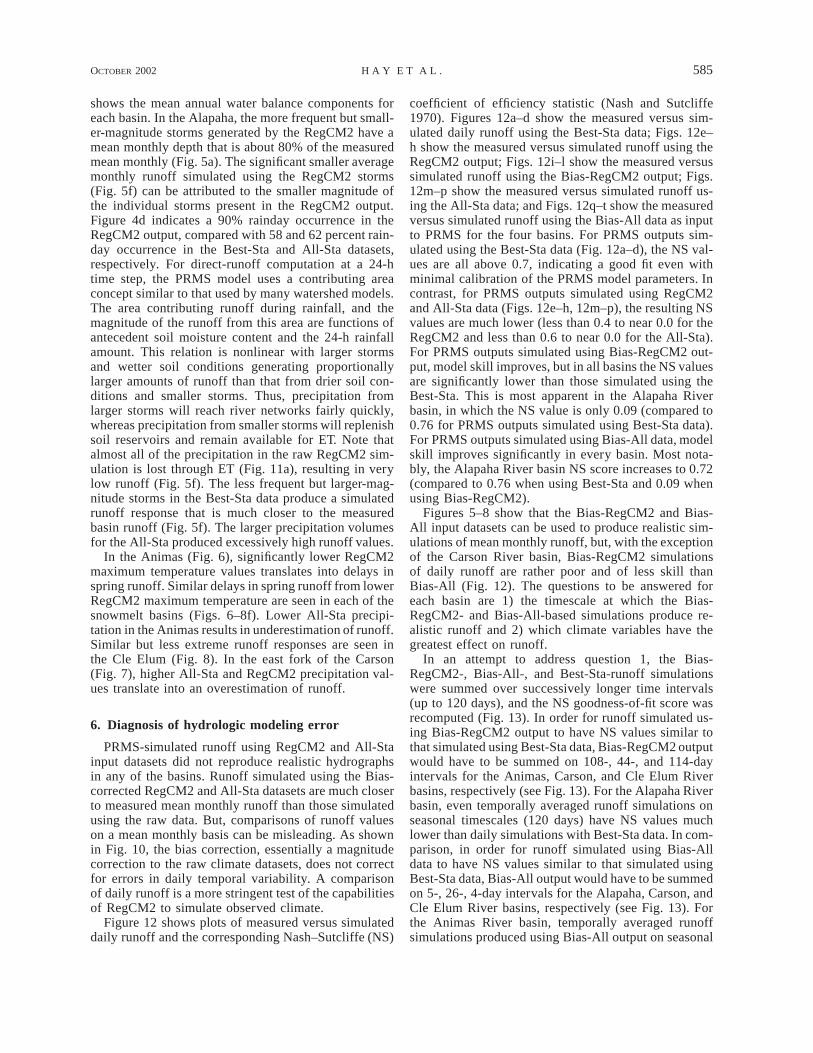
Figure 12 shows plots of measured versus simulateddaily runoff and the corresponding Nash–Sutcliffe (NS)

coefficient of efficiency statistic (Nash and Sutcliffe1970). Figures 12a–d show the measured versus sim-ulated daily runoff using the Best-Sta data; Figs. 12e–h show the measured versus simulated runoff using theRegCM2 output; Figs. 12i–l show the measured versussimulated runoff using the Bias-RegCM2 output; Figs.12m–p show the measured versus simulated runoff us-ing the All-Sta data; and Figs. 12q–t show the measuredversus simulated runoff using the Bias-All data as inputto PRMS for the four basins. For PRMS outputs sim-ulated using the Best-Sta data (Fig. 12a–d), the NS val-ues are all above 0.7, indicating a good fit even withminimal calibration of the PRMS model parameters. Incontrast, for PRMS outputs simulated using RegCM2and All-Sta data (Figs. 12e–h, 12m–p), the resulting NSvalues are much lower (less than 0.4 to near 0.0 for theRegCM2 and less than 0.6 to near 0.0 for the All-Sta).For PRMS outputs simulated using Bias-RegCM2 out-put, model skill improves, but in all basins the NS valuesare significantly lower than those simulated using theBest-Sta. This is most apparent in the Alapaha Riverbasin, in which the NS value is only 0.09 (compared to0.76 for PRMS outputs simulated using Best-Sta data).For PRMS outputs simulated using Bias-All data, modelskill improves significantly in every basin. Most nota-bly, the Alapaha River basin NS score increases to 0.72(compared to 0.76 when using Best-Sta and 0.09 whenusing Bias-RegCM2).

Figures 5–8 show that the Bias-RegCM2 and Bias-All input datasets can be used to produce realistic sim-ulations of mean monthly runoff, but, with the exceptionof the Carson River basin, Bias-RegCM2 simulationsof daily runoff are rather poor and of less skill thanBias-All (Fig. 12). The questions to be answered foreach basin are 1) the timescale at which the Bias-RegCM2- and Bias-All-based simulations produce re-alistic runoff and 2) which climate variables have thegreatest effect on runoff.

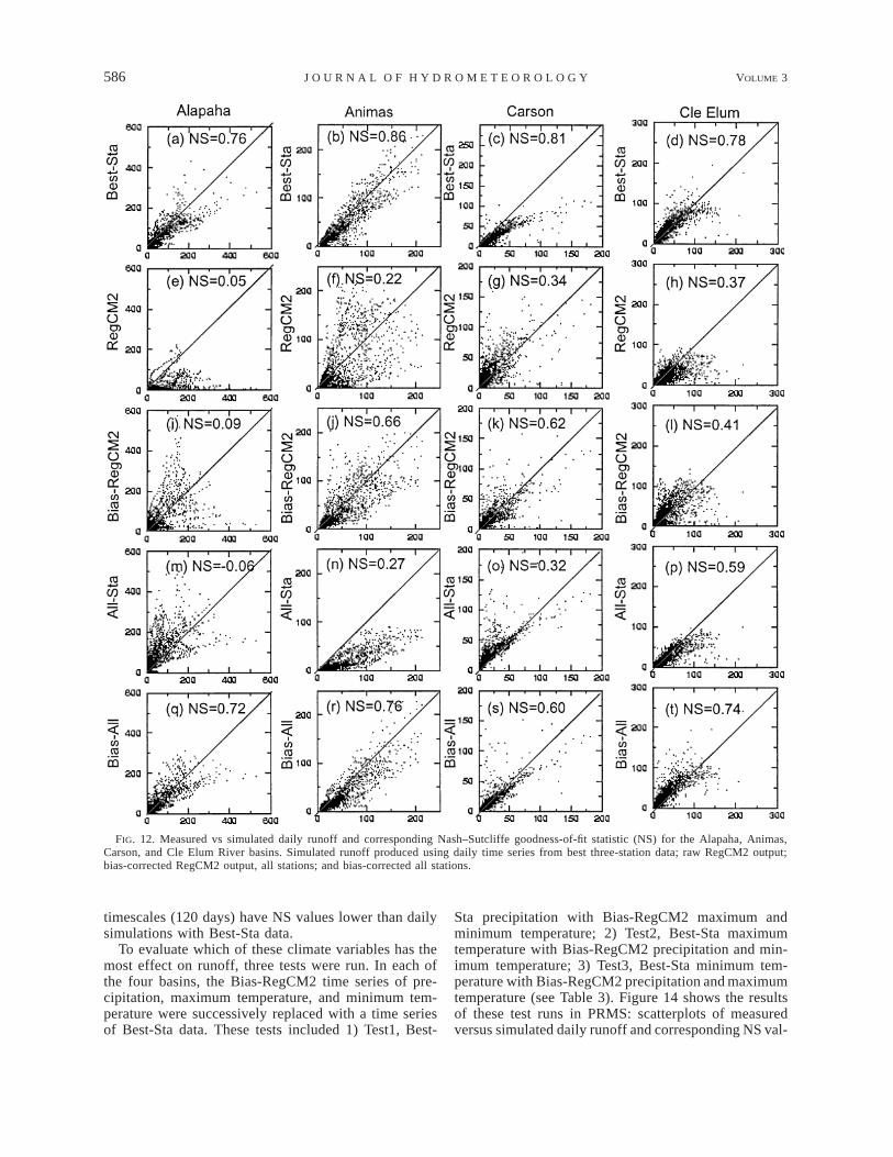
In an attempt to address question 1, the Bias-RegCM2-, Bias-All-, and Best-Sta-runoff simulationswere summed over successively longer time intervals(up to 120 days), and the NS goodness-of-fit score wasrecomputed (Fig. 13). In order for runoff simulated us-ing Bias-RegCM2 output to have NS values similar tothat simulated using Best-Sta data, Bias-RegCM2 outputwould have to be summed on 108-, 44-, and 114-dayintervals for the Animas, Carson, and Cle Elum Riverbasins, respectively (see Fig. 13). For the Alapaha Riverbasin, even temporally averaged runoff simulations onseasonal timescales (120 days) have NS values muchlower than daily simulations with Best-Sta data. In com-parison, in order for runoff simulated using Bias-Alldata to have NS values similar to that simulated usingBest-Sta data, Bias-All output would have to be summedon 5-, 26-, 4-day intervals for the Alapaha, Carson, andCle Elum River basins, respectively (see Fig. 13). Forthe Animas River basin, temporally averaged runoffsimulations produced using Bias-All output on seasonal


FIG. 12. Measured vs simulated daily runoff and corresponding Nash–Sutcliffe goodness-of-fit statistic (NS) for the Alapaha, Animas,Carson, and Cle Elum River basins. Simulated runoff produced using daily time series from best three-station data; raw RegCM2 output;bias-corrected RegCM2 output, all stations; and bias-corrected all stations.

timescales (120 days) have NS values lower than dailysimulations with Best-Sta data.

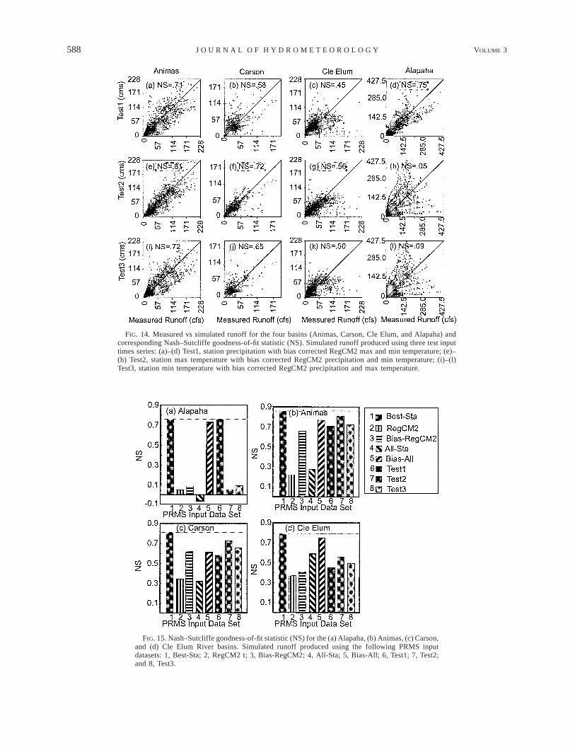
To evaluate which of these climate variables has themost effect on runoff, three tests were run. In each ofthe four basins, the Bias-RegCM2 time series of pre-cipitation, maximum temperature, and minimum tem-perature were successively replaced with a time seriesof Best-Sta data. These tests included 1) Test1, Best-

Sta precipitation with Bias-RegCM2 maximum andminimum temperature; 2) Test2, Best-Sta maximumtemperature with Bias-RegCM2 precipitation and min-imum temperature; 3) Test3, Best-Sta minimum tem-perature with Bias-RegCM2 precipitation and maximumtemperature (see Table 3). Figure 14 shows the resultsof these test runs in PRMS: scatterplots of measuredversus simulated daily runoff and corresponding NS val-


FIG. 13. Nash–Sutcliffe goodness-of-fit (NS) values calculated forthe (a) Alapaha, (b) Animas, (c) Carson, and (d) Cle Elum Riverbasins. NS values were calculated between measured and simulatedrunoff values summed on 1-, 5-, 15-, 30-, 60-, 90-, and 120-dayintervals.

ues. The highest NS values are highlighted on the plots.What becomes evident from Fig. 14 is the importanceof temperature in the snowmelt basins (Test2 gives thehighest NS values) and precipitation in the rainfall-dom-inated basin (Test1 gives the highest NS values).

7. Discussion

This study was initiated to examine possibilities forusing regional climate model output in hydrologic ap-plications. Three initial daily datasets were composedfrom 1) best precipitation and temperature station setsfor each basin determined through hydrologic modelcalibration (Best-Sta); 2) RegCM2 output; and 3) allstations (excluding Best-Sta sets) that fell within thebuffered area used to extract the RegCM2 output (All-Sta). The Best-Sta datasets simulated realistic daily hy-drographs in all four study basins. All-Sta datasets weretested to determine if an area as large as that coveredby the RegCM2 grid points could produce realistic pre-cipitation and temperature for basin-scale modeling.Both the All-Sta data and RegCM2 output of precipi-tation, maximum temperature, and minimum tempera-ture produced unrealistic simulations of runoff in allfour study basins when used as input to the hydrologicmodel. Bias corrections to the RegCM2 output and All-

Sta data produced the next two input datasets: 4) Bias-RegCM2 and 5) Bias-All. Use of Bias-RegCM2 andBias-All in PRMS resulted in more realistic monthlymean hydrographs, but comparison of daily valuesshowed that with the exception of one basin (Carson),Bias-RegCM2 output was still not nearly as reliable insimulating daily runoff as Bias-All. The final three inputdatasets (Test1, Test2, and Test3) were produced to testwhich climate variables had the most effect on runoff.These tests clearly showed the significance of realistictemperature data in the snowmelt basins and realisticprecipitation in the rainfall-dominated basins.

A summary of NS results produced using the eightinput datasets in PRMS is shown in Fig. 15. Not sur-prisingly, Best-Sta data outperformed any of the otherPRMS input datasets. In the Alapaha River basin, theonly other PRMS input datasets that simulated realistichydrographs were Test1 and Bias-All, highlighting thesignificance of realistic precipitation in this southeasternUnited States basin and the relative reduced significanceof maximum and minimum temperature. The fact thatBias-All dramatically outperforms Bias-RegCM2 in thisrainfall-dominated basin also indicates that precipitationaveraged over a large area can have the daily variationsnecessary for basin-scale modeling. On the other hand,snowmelt-dominated basins are much more stronglycontrolled by maximum temperature. In these basins,daily variations in precipitation are less important, andonly the volume of precipitation over the accumulationseason (e.g., as represented in the 1 April snowpack)needs to be correct.

These results are consistent with Wilby and Dettin-ger’s (2000) study of snowmelt-dominated basins in theSierra Nevada. In their study they concluded that muchof the hydrological ‘‘skill’’ arises from the fact that thesnowpack acts as an integrator of the hydrologic pro-cesses. In a sense, the Leung et al. (1996) study alsosupports these results. Leung et al. (1996) drove a spa-tially distributed hydrologic model of a snowmelt-dom-inated basin in northwestern Montana using measuredand regional climate model (RCM) output and con-cluded that runoff simulated using RCM output resultedin comparable, if not better, agreement with measuredrunoff than driving the model with measured data. Intheir study, measured data from two stations was dis-tributed by assuming a constant lapse rate with altitude.The lapse rate for temperature was set at a constant 68Ckm21. The RCM output was distributed using a subgridparametrization scheme. In our study we have shownthe importance of temperature in snowmelt dominatedbasins. The constant lapse rate used by Leung et al.(1996) to distribute the measured temperature data prob-ably affected the runoff simulations. It is likely that theirsubgrid parametrization scheme corrected the biases inthe RegCM2 temperature output, thus producing morerealistic hydrographs than that using measured-temper-ature data.


FIG. 14. Measured vs simulated runoff for the four basins (Animas, Carson, Cle Elum, and Alapaha) andcorresponding Nash–Sutcliffe goodness-of-fit statistic (NS). Simulated runoff produced using three test inputtimes series: (a)–(d) Test1, station precipitation with bias corrected RegCM2 max and min temperature; (e)–(h) Test2, station max temperature with bias corrected RegCM2 precipitation and min temperature; (i)–(l)Test3, station min temperature with bias corrected RegCM2 precipitation and max temperature.

FIG. 15. Nash–Sutcliffe goodness-of-fit statistic (NS) for the (a) Alapaha, (b) Animas, (c) Carson,and (d) Cle Elum River basins. Simulated runoff produced using the following PRMS inputdatasets: 1, Best-Sta; 2, RegCM2 t; 3, Bias-RegCM2; 4, All-Sta; 5, Bias-All; 6, Test1; 7, Test2;and 8, Test3.


8. Conclusions

Daily precipitation and maximum and minimum tem-perature time series from a regional climate model(RegCM2) were used as input to a distributed hydro-logic model for three snowmelt-dominated basins (An-imas River at Durango, Colorado; east fork of theCarson River near Gardnerville, Nevada; and Cle ElumRiver near Roslyn, Washington) and a rainfall-domi-nated basin (Alapaha River at Statenville, Georgia). Forcomparison purposes, daily datasets of precipitation andmaximum and minimum temperature were developedusing measured station data that fell within the area usedto extract the RegCM2 output (All-Sta). The All-Stadatasets are comparable in scale to the RegCM2 modelresolution and provide an appropriate test to determineif output at this scale can be used for simulation of basin-scale hydrology.

Both the RegCM2 and All-Sta simulations capturethe gross aspects of the seasonal cycles of precipitationand temperature. However, in all four basins large sys-tematic biases in RegCM2 and All-Sta simulations oftemperature and precipitation are evident, which trans-late into unrealistic simulations of mean-monthly hy-drographs. In order to reproduce realistic mean-monthlyhydrographs in each of the four basins studied, theRegCM2 and All-Sta output are corrected for biases(Bias-RegCM2 and Bias-All, respectively).

Simulated runoff based on Bias-RegCM2 output andBias-All data were evaluated on a monthly and dailybasis. On a mean monthly basis, runoff simulated usingthe Bias-RegCM2 and Bias-All sets are much closer tomeasured runoff than those simulated using the rawdata. On a daily basis, with the exception of the CarsonRiver basin, Bias-RegCM2-based simulations are ratherpoor and of less skill than Bias-All. Most notable arethe results in the rainfall-dominated basin: Bias-RegCM2-based simulations show essentially no skillwhereas Bias-All-based simulations reproduce realisticrunoff. These results indicate that precipitation averagedover a large area can have the daily variations necessaryfor basin-scale modeling. In the snowmelt-dominatedbasins, which are strongly controlled by maximum tem-perature, capturing daily variations in precipitation wasfound to be less important, and only the volume ofprecipitation over the accumulation season needs to becorrect.

In conclusion, climate data of similar resolution tothat of the RegCM2 model can be made appropriate forbasin-scale modeling when a bias correction is applied.This need for statistical correction (essentially a mag-nitude correction) may be somewhat troubling, but inthe case of the large station dataset (All-Sta), the mag-nitude correction did indeed correct for the change inscale. This was not shown to be true for the bias-cor-rected RegCM2 output. The RegCM2 output could becorrected for magnitude but did not contain the day-to-day variability needed for basin-scale modeling present

in the All-Sta dataset. The major advantage of usingregional climate model output to simulate runoff is theirphysical realism. It is unknown if statistical correctionsto model output will be valid in a future climate. Futurework is warranted to identify the causes for (and re-moval of ) systematic biases in RegCM2 simulations,and to improve RegCM2 simulations of daily variabilityin local climate.

REFERENCES

Anderson, J. R., E. E. Hardy, J. T. Roach, and R. E. Witmer, 1976:A land use land cover classification system for use with remotesensor data. U.S. Geological Survey Prof. Paper 964, 28 pp.

Briegleb, B. P., 1992: Delta-Eddington approximation for solar ra-diation in the NCAR Community Climate Model. J. Geophys.Res., 97, 7603–7612.

Dickinson, R. E., A. Henderson-Sellers, and P. J. Kennedy, 1992:Biosphere–Atmosphere Transfer Scheme (BATS) version 1e ascoupled to NCAR Community Climate Model. NCAR Tech.Note 3871STR, 72 pp.

Giorgi, F., L. O. Mearns, C. Shields, and L. Mayer, 1996: A regionalmodel study of the importance of local versus remote controlsof the 1988 drought and the 1993 flood over the central UnitedStates. J. Climate, 9, 1150–1161.

Grell, G. A., 1993: Prognostic evaluation of assumptions used bycumulus parameterizations. Mon. Wea. Rev., 121, 764–787.

Hay, L. E., and M. P. Clark, 2000: Use of atmospheric forecasts inhydrologic models in mountainous terrain. Part 2: Applicationto hydrologic models. Proc. AWRA Spring Specialty Conf. onWater Resources in Extreme Environments, Anchorage, AK,American Water Resources Association, 221–226.

——, R. L. Wilby, and G. H. Leavesley, 2000: A comparison of deltachange and downscaled GCM scenarios for three mountainousbasins in the United States. J. Amer. Water Resour. Assoc., 36,387–397.

Holtslag, A. A. M., E. I. F. de Bruijn, and H. L. Pan, 1990: A highresolution air mass transformation model for short-range weatherforecasting. Mon. Wea. Rev., 118, 1561–1575.

Hsie, E.-Y., R. A. Anthes, and D. Keyser, 1984: Simulations of front-ogenesis in a moist atmosphere using alternative parameteriza-tions of condensation and precipitation. J. Atmos. Sci., 41, 2701–2716.

Kalnay, E., and Coauthors, 1996: The NCEP/NCAR 40-Year Re-analysis Project. Bull. Amer. Meteor. Soc., 77, 437–471.

Leavesley, G. H., and L. G. Stannard, 1995: The precipitation–runoffmodeling system—PRMS. Computer Models of Watershed Hy-drology, V. P. Singh, Ed., Water Resources Publications, 281–310.

——, R. W. Lichty, B. M. Troutman, and L. G. Saindon, 1983: Pre-cipitation–runoff modeling system: User’s manual. Rep. 83-4238, U.S. Geological Survey Water Investigation, 207 pp.

——, M. D. Branson, and L. E. Hay, 1992: Using coupled atmo-spheric and hydrologic models to investigate the effects of cli-mate change in mountainous regions. Managing Water Resourc-es During Global Change. AWRA 28th Annual Conference andSymposium, R. Herrmann, Ed., American Water Resources As-sociation, 691–700.

——, L. E. Hay, R. J. Viger, and S. L. Markstrom, 2002a: Use ofobjective distributed-parameter estimation methods to constrainmodel calibration. Advances in Calibration of Watershed Mod-els, Geophys. Monogr., Amer. Geophys. Union, in press.

——, S. L. Markstrom, P. J. Restrepo, and R. J. Viger, 2002b: Amodular approach to addressing model design, scale, and pa-rameter estimation issues in distributed hydrological modeling.Hydrol. Processes, 16, 173–187.

Leung, L. R., M. S. Wigmosta, S. J. Ghan, D. J. Epstein, and L. W.Vail, 1996: Application of a subgrid orographic precipitation/


surface hydrology scheme to a mountain watershed. J. Geophys.Res., 101 (D8), 12 803–12 817.

Milly, P. C. D., and K. A. Dunne, 2002: Macro-scale water fluxes.1. Quantifying errors in the estimation of river-basin precipita-tion. Water Resour. Res., in press.

Nash, J. E., and J. V. Sutcliffe, 1970: River flow forecasting throughconceptual models. Part I: A discussion of principles. J. Hydrol.,10, 282–290.

Panofsky, H. A., and G. W. Brier, 1968: Some Applications of Sta-tistics to Meteorology. The Pennsylvania State University Press,224 pp.

Phillips, T. J., 1995: Documentation of the AMIP models on the WorldWide Web. UCRL-MI-116384, Lawrence Livermore Laboratory,14 pp.

Ramage, C. S., 1983: Teleconnections and the siege of time. J. Cli-matol., 3, 223–231.

Sevruk, B., 1989: Reliability of precipitation measurements. WMO/IAHS/ETH Workshop on Precipitation Measurements, Zurich,Switzerland, Dept. of Oceanography, Swiss Federal Institute ofTechnology, 13–19.

Takle, E. S., and Coauthors, 1999: Project to Intercompare RegionalClimate Simulations (PIRCS): Description and initial results. J.Geophys. Res., 104, 19 443–19 461.

U.S. Department of Agriculture, cited 2002: Forest land distributiondata for the United States: Forest Service. [Available online athttp://www.srsfia.usfs.msstate.edu/rpa/rpa93.htm.]

——, 1994: State Soil Geographic (STATSGO) database—Data useinformation. Misc. Publ. 1492, Natural Resources ConservationService, 107 pp.

Watson, R. T., M. C. Zinyowera, and R. H. Moss, 1996: ClimateChange 1995: Impacts, Adaptations, and Mitigations of ClimateChange. Cambridge University Press, 889 pp.

Wilby, R. L., and M. D. Dettinger, 2000: Streamflow changes in theSierra Nevada, CA, simulated using statistically downscaled gen-eral circulation model output. Linking Climate Change to LandSurface Change, S. McLaren, and D. Kniveton, Eds., KluwerAcademic, 99–121.

——, L. E. Hay, and G. H. Leavesley, 1999: A comparison of down-scaled and raw GCM output: Implications for climate changescenarios in the San Juan River Basin, Colorado. J. Hydrol., 225,67–91.

——, ——, W. J. Gutowski, R. W. Arritt, E. S. Takle, Z. Pan, G. H.Leavesley, and M. P. Clark, 2000: Hydrological responses todynamically and statistically downscaled climate model output.Geophys. Res. Lett., 27, 1199–1202.

Wilks, D. S., 1995: Statistical Methods in the Atmospheric Sciences:An Introduction. Academic Press, 467 pp.

Documents

Use of Regional Climate Model Output for Hydrologic ...sciencepolicy.colorado.edu/admin/publication_files/resource-127-2002.30.pdfb. Regional climate model output The RCM output was