Embed Size (px)
Citation preview
Use of Membranes in Gas Conditioning
Hope Baumgarner
Chelsea Ryden
Professor Dr. Miguel Bagajewicz
8 May 2009
Executive Summary
Natural gas processing is one of the largest industrial gas separation applications
worldwide and is on the verge of innovative technology which may prove more economically
sound. One such technology is membrane networks which compete directly with amine units to
separate carbon dioxide from natural gas. Currently, membrane networks consisting of multiple
membranes, compressors, mixers and splitters are being investigated to determine whether these
systems can handle larger flow rates than membrane units at a reduced cost.
A model was designed in GAMS to assess the feasibility of an amine unit versus a
membrane network where the annual processing cost was minimized. Several membrane
networks processing natural gas at 19% CO2 were designed to determine the optimal network.
The two membrane network resulted in an annual processing cost of $163K with a total of 11%
methane lost. A four membrane network was run in GAMS resulting in the three membrane
network which was the optimal solution. The three membrane network had the smallest annual
processing cost of $130K with 7.77% methane lost. Furthermore, the three membrane network
was scaled up at varying flow rates with 19% and 9% CO2 to compare the operating cost and
total annualized cost to the amine unit’s. At flow rates less than 270 MMscfd (19% CO2) the
membrane network had lower operating costs ranging from $175K to $39MM and a total
annualized cost ranging from $202K to $45MM. At the same flow rates, the amine unit had
operating costs ranging from $490K to $37MM and a total annualized cost ranging from $532K
to $38MM. For the 9% CO2 case, the membrane network had a lower operating cost of $16MM
and a total annualized cost of $17MM at a flow rate below 150MMscfd. At the same flow rate
and CO2 concentration, the amine unit’s operating cost and total annualized cost were $16.5MM
and $17.5MM. It is recommended that membrane networks be used in applications with high
CO2 concentrations at flow rates less than 270 MMscfd.

Table of Contents
1.Introduction ............................................................................................................................................... 2
2. Natural Gas Processing ............................................................................................................................. 2
3. Membrane Theory .................................................................................................................................... 4
4. Membrane Modules ................................................................................................................................. 7
4.1 Spiral-Wound ...................................................................................................................................... 8
4.2 Hollow-Fiber ........................................................................................................................................ 8
5. Commercially Available Membrane Material ........................................................................................... 9
6. Investigated Membrane Material ........................................................................................................... 11
7. Membrane Advantages ........................................................................................................................... 12
8. Membrane Disadvantages ...................................................................................................................... 14
9. Membrane Applications .......................................................................................................................... 15
10. Amine Unit ............................................................................................................................................ 16
11. Development of Model ......................................................................................................................... 18
11.1 Comparison between GAMS and Excel results ............................................................................... 18
11.2 Membrane Simulation Model ......................................................................................................... 20
11.3 Mixer and splitter balances ............................................................................................................. 23
11.4 Objective Function .......................................................................................................................... 26
11.5 Discrete Method ............................................................................................................................. 28
12. Results ................................................................................................................................................... 29
12.1 Comparison Between Various Membrane Networks ..................................................................... 30
12.2 Assessment of Amine Unit to Membrane Network ........................................................................ 30

13. Recommendations ................................................................................................................................ 32
References .................................................................................................................................................. 36
Appendix I ................................................................................................................................................... 37
2
1. Introduction
Roughly 550 trillion scf (standard cubic feet) of natural gas in the lower 48 states cannot
be processed because of high CO2 content. Membrane networks for gas conditioning have the
potential to process this low quality natural gas. Carbon dioxide, which is an acid gas, is
commonly found in natural gas streams at levels as high as 50%. It is corrosive which rapidly
destroys pipelines unless it is removed. Some common techniques for acid gas removal include
absorption processes, cryogenic processes, adsorption processes and membrane separation.
Membrane gas separation techniques were first introduced in the 1980’s, and since then
membrane based gas separation has developed into a $150 million per year business (Kookos,
193). Membranes are increasingly being used in applications which have larger flow rates and
high CO2 content.
The total worldwide consumption of natural gas is roughly 95 trillion scf/yr. The
increased consumption of natural gas is the driver for innovative technology due to the high cost
of equipment which is roughly $5 billion per year. However, membranes have less than five
percent of this market (Baker, 2109). This paper summarizes current natural gas processing,
membrane theory, optimization of membrane networks and a cost analysis between an amine
unit and a three membrane network.
2. Natural Gas Processing
Current natural gas processing techniques require a number of steps prior to consumer
usage. Although raw natural gas is primarily composed of methane, other impurities such as
hydrogen sulfide, carbon dioxide, nitrogen, water vapor and helium are also present. Moreover,
raw natural gas is commonly mixed with hydrocarbons such as ethane, propane, and butane
which are valuable by products when separated. Prior to the distribution of natural gas, it must
3
be processed to meet federal regulations which specify the composition of the sale gas.
According to these pipeline regulations, the sale gas must contain less than 2% carbon dioxide
and trace amounts of water vapor, hydrogen sulfide, nitrogen and other hydrocarbons. These
stringent guidelines are aimed at reducing pollutant emissions as well as reducing the amount of
corrosive components like carbon dioxide and hydrogen sulfide from damaging pipe lines.
The series of steps involved in natural gas processing consist of oil and condensate
removal, acid gas removal, dehydration, nitrogen rejection, natural gas liquid separation, and
fractionation. In order to transport and process natural gas, the oil in which it is dissolved in has
to be removed. This typically takes place at or near the well head. In some instances, the
separation of natural gas and oil will occur on its own during production due to decreased
pressure. In this case, a conventional separator uses the force of gravity to separate the natural
gas from the oil. However, sometimes specialized equipment such as a low temperature separator
is used to remove any oil from the natural gas. This piece of equipment uses pressure
differentials throughout different sections of the separator creating temperature variation. As a
result, oil and some water vapor are condensed out of the wet gas stream. Once this separation is
achieved, the raw natural gas is sent to an acid gas removal unit also known as an amine unit.
Here the natural gas which contains relatively high levels of carbon dioxide and hydrogen sulfide
is treated with an amine solution. As the sour gas runs through the tower, carbon dioxide and
sulfur are removed because of the amine solution’s affinity for the two. The most commonly
used amine solutions are monoethanolamine (MEA) and diethanolamine (DEA). Typically, the
sulfur which was removed from the sour gas is sent to a Claus unit where it is converted into
elemental sulfur. After the natural gas has been sweetened, it is sent to a dehydration unit to
remove the existing water vapor using either adsorption or absorption. During absorption a
4
drying agent such as diethylene glycol or triethylene glycol comes into contact with the wet
natural gas removing the water vapor. Adsorption differs from absorption because a solid
desiccant which also promotes drying is used to collect the water vapor from the wet gas onto its
surface. Next, nitrogen is removed from the natural gas using a cryogenic, adsorption, or
absorption process. During cryogenic expansion, the temperature of the gas stream is dropped to
around -120 ºF using a turbo expander. This allows some components in the gas stream to
condense while leaving methane in a gaseous state. Prior to the sale of natural gas, the natural
gas liquids must be removed using either a cryogenic expansion process or absorption process.
Once the natural gas liquids have been recovered from the gas stream, they are sent to a
fractionation unit in order to separate the by-product into its individual constituents such as
ethane, propane, and butane. The technology used in natural gas processing has not seen much
change in the past few decades; however, advances in natural gas production may prove
beneficial to this industry.
3. Membrane Theory
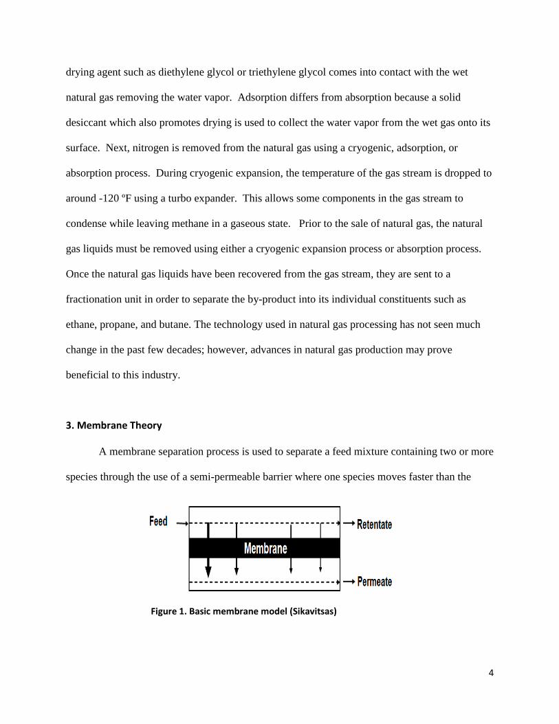
A membrane separation process is used to separate a feed mixture containing two or more
species through the use of a semi-permeable barrier where one species moves faster than the
Figure 1. Basic membrane model (Sikavitsas)

5
other. Figure 1 depicts the most general membrane separation process in which the feed is
separated into a retentate and permeate. The retentate is termed the slow gas as it does not pass
through the membrane while the permeate is termed the fast gas as it passes through the
membrane. The following membrane theory was referenced from Seader and Henley.
Mass transport through membranes is described by Fick’s Law
�� � ���� �� � � � (1)
where �� is the molar flux of species i, �� is the diffusivity of component i, �� is the membrane
thickness, �� is the concentration of component i at the feed membrane interface and � is the
concentration of component i at the permeate membrane interface (see Figure 2). However,
Fick’s Law is not valid at the interface. Therefore, thermodynamic equilibrium is assumed so
that Fick’s Law can be related to the partial pressures through Henry’s Law
��� � �� ���� (2)
�� � � �� � (3) where the subscripts � and � refer to the feed membrane interface and membrane permeate
interface, respectively, � is the concentration of component i, �� is the partial pressure of
component i and �� is solubility constant.
Figure 1 Figure 2. Membrane concentration profile (Sikavitsas)
6
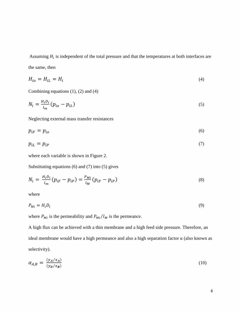
Assuming �� is independent of the total pressure and that the temperatures at both interfaces are
the same, then
��� � �� � �� (4)
Combining equations (1), (2) and (4)
�� � ������ ��� � �� � (5)
Neglecting external mass transfer resistances
��� � ��� (6)
�� � ��� (7)
where each variable is shown in Figure 2.
Substituting equations (6) and (7) into (5) gives
�� � ������ ��� � ���� � ����� ��� � ���� (8)
where
��� � ���� (9) where ��� is the permeability and ��� ��⁄ is the permeance.
A high flux can be achieved with a thin membrane and a high feed side pressure. Therefore, an
ideal membrane would have a high permeance and also a high separation factor α (also known as
selectivity).
��,! � "# $#⁄ �"% $&⁄ � (10)
7
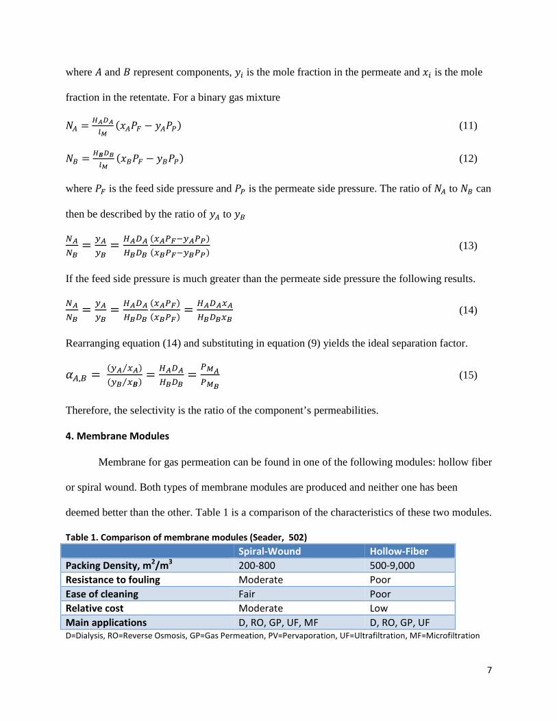
where ' and ( represent components, )� is the mole fraction in the permeate and *� is the mole
fraction in the retentate. For a binary gas mixture
�� � �#�#�� *��� � )���� (11)
�! � �&�%�� *!�� � )!��� (12)
where �� is the feed side pressure and �� is the permeate side pressure. The ratio of �� to �! can
then be described by the ratio of )� to )!
+#+% � "#"% � �#�#�%�%$#�,-"#�.�$%�,-"%�.� (13)
If the feed side pressure is much greater than the permeate side pressure the following results.
+#+% � "#"% � �#�#�%�%$#�,�$%�,� � �#�#$#�%�%$% (14)
Rearranging equation (14) and substituting in equation (9) yields the ideal separation factor.
��,! � "# $#⁄ �"% $&⁄ � � �#�#�%�% � ��#��% (15)
Therefore, the selectivity is the ratio of the component’s permeabilities.
4. Membrane Modules
Membrane for gas permeation can be found in one of the following modules: hollow fiber
or spiral wound. Both types of membrane modules are produced and neither one has been
deemed better than the other. Table 1 is a comparison of the characteristics of these two modules.
Table 1. Comparison of membrane modules (Seader, 502)
Spiral-Wound Hollow-Fiber
Packing Density, m2/m3 200-800 500-9,000
Resistance to fouling Moderate Poor
Ease of cleaning Fair Poor
Relative cost Moderate Low
Main applications D, RO, GP, UF, MF D, RO, GP, UF D=Dialysis, RO=Reverse Osmosis, GP=Gas Permeation, PV=Pervaporation, UF=Ultrafiltration, MF=Microfiltration

8
4.1 Spiral-Wound
Spiral wound modules are the least common modules which compose less than 20% of
membranes formed (Baker, 1395). Although they have a higher production cost ($10-100/m2),
this is compensated for by their high permeance and flux (Baker, 1395). Another advantage of
spiral wound modules is their ability to use a wide range of materials compared to hollow fiber
modules. Lastly, spiral wound modules are more resistant to plasticization, resulting in a longer
life span.
4.2 Hollow-Fiber
Hollow fiber membranes are the most common type of module. Hollow fiber modules
have a greater packing density, i.e., more membrane area per unit volume, than spiral wound
modules. Hollow fiber modules have a higher packing density because fine fibers can be used in
the module, therefore allowing more fibers and thus a higher packing density. As a result, hollow
fiber plants are typically smaller than spiral wound plants. Also, hollow fiber membranes tend to
Figure 3. Spiral wound membrane module (Dortmundt, 7)

9
have a lower flux than spiral wound membranes because the layer through which the gas
permeates is thicker.
The low cost ($2-5/m2) of hollow fiber modules makes it advantageous over spiral wound
modules (Baker, 1395). Although the low cost of hollow fiber modules might be appealing,
membrane modules only make up about 10-25% of the total plant cost (Baker, 1395). Therefore,
reductions in the membrane module cost may not significantly reduce the overall plant cost.
Lastly, hollow fiber membranes have the selectivities and flux required. The major
problem is the low reliability of these membranes caused by fouling. Moreover, hollow fiber
modules require more careful and expensive treatment to avoid these problems.
5. Commercially Available Membrane Material
Although several types of materials used in membranes exist, it is essential that the
material used be appropriate for the application. Some parameters to consider when selecting an
appropriate material are selectivity, cost, and durability. In general, the major cost factor in
Figure 4. Hollow fiber membrane module (Dortmundt, 8)

10
membrane networks is not the material. In the case of natural gas processing, the membrane
material must be able to withstand the operating conditions. For example, the material of interest
should be able to remain stable in the presence of components such as benzene, toluene,
ethybenzene, and xylene. Even though it is not typical for membrane networks to operate under
substantially high flow rates compared to current natural gas processing units, the material’s
performance should not be hindered by varying conditions such as temperature, pressure and gas
composition.
A membrane material’s degree of selectivity is crucial for adequate separation to occur.
A common membrane material used in industry is known as cellulose acetate. One of the
reasons it is favored in industry is because it has a high selectivity for carbon dioxide over
methane, and it is stable in the presence of most organic solvents. Membrane materials used for
natural gas processing are classified according to the type of polymer in which they are
constructed from. In the case of cellulose acetate, the polymer which comprises this material is
known as a glassy polymer. The structure of a glassy polymer is rigid and tough because it is
below the glass transition temperature. As a result, the polymer chains have limited mobility
causing the membrane to discriminate between molecules based on size. Furthermore, polymers
above their glass transition point are termed rubbery polymers. Some examples of commercially
available rubbery polymers are silicone rubber and amide block co-polymers. Rubbery polymers
differ from glassy polymers in that the polymer chains are more mobile and the material is more
elastic. This difference allows membranes composed of rubbery polymers to separate
components based on condensability. Condensability is the ease at which a gas is able to
transition from a gaseous state to a liquid state onto the surface of the membrane material
allowing it to be collected separately. In order to determine the type of polymer which is best
11
suited to separate a desired component from a gas mixture, it is vital to evaluate the physical
properties of the polymer. For example, glassy polymers are typically used to separate carbon
dioxide from methane because they separate based on size. However, rubbery polymers can be
used when one component condenses more readily than another which is the case for the
separation between hydrogen sulfide and carbon dioxide. The properties of the membrane
material are crucial in determining its performance, degree of selectivity, cost and durability.
6. Investigated Membrane Material
Cellulose acetate is one of the most common polymers used in membrane material for
natural gas processing, but compared to other investigated material its selectivity for hydrogen
sulfide over methane is inferior. Some examples of new polymeric membranes include
polydimethylsiloxane, pebax, poly(ether/ester urethane), poly(sulfone), and poly(butadiene).
These polymeric membranes have been studied for the purpose of acid gas applications and
based on some experimental results have a significantly higher selectivity for hydrogen sulfide
compared to cellulose acetate. In a study conducted to determine the permeation behavior of
CO2, H2S and CH4 in poly (ester urethane urea), selectivities of 43 and 16 were measured for
H2S/CH4 and CO2/CH4 (Mohammadi 7361). At the same experimental conditions, the
selectivities for H2S/CH4 and CO2/CH4 in cellulose acetate were 22 and 19 (Mohammadi 7361).
These results demonstrate the potential for polymeric membranes in acid gas removal, but some
draw backs such as plasticization and thermal stability have postponed further implementation.
Plasticization occurs when the polymer within the membrane begins to swell due to the sorption
of carbon dioxide. This decreased performance causes the membrane to lose its selectivity
properties. These issues have accelerated further investigation into plasticization resistant
material. Based on recent studies, silver incorporated pebax was shown to be resistant to

12
plasticization and its measured selectivities for CO2/CH4 and H2S/CH4 were 13 and 50 (Sridhar
8144). The addition of silver to pebax enhanced some of its properties such as its diffusive
selectivity which favors the transport of CO2. Moreover, this material demonstrated hydrophilic
behavior and was able to remove water vapor in the gas mixture at a relatively rapid rate. Other
issues with polymeric membranes are the two opposing effects of high feed pressures on the
permeation rate inside the membrane. The increased feed pressure can increase the free volume
available, thus increasing the permeation rate. However, increased feed pressure also provokes
membrane compression which decreases the free volume and decreases the permeation rate.
Recent studies have been conducted to address these issues and with further exploration into
these limitations solutions are bound to arise.
7. Membrane Advantages
High Concentration Gas
Membrane plants are more efficient at treating high concentration gas streams than lower
concentration gas streams. A membrane plant designed to treat 5 million scfd of gas that contains
20% carbon dioxide would be less than half the size of a membrane plant designed to treat 20
million scfd of gas that contains 5% carbon dioxide (Baker, 2113).
Small Gas Flow
Membrane plants have simple flow schemes, which make them preferable when
processing small gas flows. Also, membrane plants which are processed at lower flow rates of
less than 20 million scfd of gas are designed so that operators are not needed (Baker, 2113).
Lower Capital Cost
Membrane systems are housed in skids. Skid mounted membrane plants allow for more
area to be packed into a smaller volume as shown in Figure 5. Therefore minimal cost and time

13
are necessary to prepare the site. Moreover, installation costs are significantly lower than those
for alternative technologies.
Operational simplicity
Single stage membrane systems are very simple to operate because they require minimal
downtime. If upsets do not occur, they are able to operate unattended for a significant amount of
time. While single stage membranes do not require staffing, multiple stage membrane systems
only require a minimal amount. Multiple stage membrane functions, such as start up, operation
and shutdown, can be easily controlled from a control room.
Space efficiency
Figure 6 displays the space efficiency of skids. Membrane units can be assembled into
compact modules, resulting in minimal space requirements. Membrane skids are advantageous
and very common on offshore environments where space efficiency is necessary.
Figure 5. A CO2 membrane separation plant. This is a 9
million scfd membrane plant designed to reduce a 6%
CO2 gas to 2%. (Baker, 2113)
Figure 6. The skid in the lower left replaced all the
units to the right (Dortmundt, 25)

14
Design Efficiency
Dehydration and CO2 and H2S removal are integrated into one operation in membrane
systems. In traditional CO2 removal technologies, these operations are performed in multiple
stages.
Reduced Power & Consumption
Membrane systems greatly reduce the electric power and fuel consumption compared to
conventional separation techniques.
Eco-friendly
Membrane systems are environmentally friendly as the permeate gases can be re-injected
into the well or used as fuel.
8. Membrane Disadvantages
Plasticization
Membrane materials absorb 30-50 cm3 of CO2/cm3 polymer. This results in a sharp drop
in the polymer glass transition temperature and therefore a decrease in selectivity (Baker, 2114).
Physical Aging
The glassy polymers are in a non equilibrium state and over time the polymer chains
relax, resulting in a decrease in permeability (Baker, 2114).
High Skid Cost
The cost of the membrane is a small fraction of the total skid cost. The membrane module
cost often only makes up about 10-25% of the total cost (Kookos, 193). Moreover, reductions in
membrane cost may not significantly change the total plant cost. Skid costs are high because of
the large required compressor power. One way to lower the membrane skid cost is to increase the

15
permeance of the membrane. This allows a smaller membrane area to be used to treat the same
volume of gas. Another way to lower the membrane skid cost is to increase the feed gas pressure.
As a result, the area and skid size is reduced. Consequently, this increases the energy
consumption as larger compressors are necessary.
9. Membrane Applications
Within the past fifty years, membrane technology has been used in a myriad of
applications such as reverse osmosis, gas separation, and alcohol dehydration. It was in the mid
1960’s that a common membrane material today, cellulose acetate, was used to desalinize
saltwater to produce drinkable water with less than 500 ppm of solids (Seader, 493). Later in
1979, Monsanto Chemical Company used hollow-fiber membranes comprised of polysulfone to
enrich streams containing hydrogen and carbon dioxide (Seader, 493). Furthermore, the
commercialization of alcohol dehydration led to the use of membrane technology as well as the
need to remove metals and organics from waste water (Seader, 493). Although membrane
networks have been used in a variety of fashions, one of the more pertinent applications has been
its introduction into natural gas processing.
Due to the high volume of natural gas consumed worldwide, ~95 trillion scf/yr, natural
gas processing is one of the largest industrial gas separation applications (Baker, 2109).
Membrane processes make up less than five percent of natural gas processing equipment. One of
the primary reasons membrane processes are used in natural gas processing is for carbon dioxide
removal. Therefore, membrane technology competes directly with amine units which are
primarily used to remove corrosive components such as carbon dioxide and hydrogen sulfide.
Amine units are well received in the natural gas processing industry; however, many limitations
such as high maintenance issues and well monitored operating procedures restrict the use of
16
amine treatment units in remote locations. In the 1980’s, the use of membrane networks for
carbon dioxide removal became appealing in remote areas where constant monitoring was not
available. Some of the first companies to operate a membrane system to separate carbon dioxide
from natural gas were Grace Membrane Systems, Separex, and Cynara (Baker, 2110). At this
time, one of the most commonly used polymers was cellulose acetate, but within the past ten
years other membrane materials such as polyimide polymers and perfluoropolymers have
challenged its use. Recent advancements in membrane technology have made its
implementation more attractive, but this technology remains limited.
10. Amine Unit
As mentioned before, amine treatment units are typically used to remove corrosive
components in natural gas namely carbon dioxide and hydrogen sulfide. The details of this
process will be discussed in order to provide a comprehensive view of this unit. Moreover, the
inner workings of the amine treatment unit are necessary to understand the assessment of this
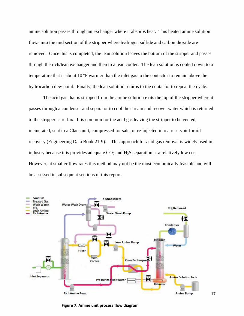
unit with the investigated membrane network. A typical process flow through an amine
treatment unit can be seen in Figure 7. First, the sour gas enters an inlet separator which
removes any liquids or solids present in the gas mixture. Once the sour gas leaves the inlet
contactor it enters the bottom of the contactor where it contacts an amine solution. During this
contact, components in the acid gas react with the amine solution to form a salt. The gas
continues to move up the column and the sweetened gas exits at the top of the column where it
passes through an outlet separator. Next, the sweetened gas must go through dehydration to
remove the excess water. The sweetened gas also goes through a water wash in order to recover
any vaporized and entrained amine solution. The rich amine solution exiting the contactor enters
a flash drum to remove the remaining hydrocarbons. After leaving the flash drum, the rich
17
amine solution passes through an exchanger where it absorbs heat. This heated amine solution
flows into the mid section of the stripper where hydrogen sulfide and carbon dioxide are
removed. Once this is completed, the lean solution leaves the bottom of the stripper and passes
through the rich/lean exchanger and then to a lean cooler. The lean solution is cooled down to a
temperature that is about 10 ºF warmer than the inlet gas to the contactor to remain above the
hydrocarbon dew point. Finally, the lean solution returns to the contactor to repeat the cycle.
The acid gas that is stripped from the amine solution exits the top of the stripper where it
passes through a condenser and separator to cool the stream and recover water which is returned
to the stripper as reflux. It is common for the acid gas leaving the stripper to be vented,
incinerated, sent to a Claus unit, compressed for sale, or re-injected into a reservoir for oil
recovery (Engineering Data Book 21-9). This approach for acid gas removal is widely used in
industry because it is provides adequate CO2 and H2S separation at a relatively low cost.
However, at smaller flow rates this method may not be the most economically feasible and will
be assessed in subsequent sections of this report.
Figure 7. Amine unit process flow diagram
Figure 7. Amine unit process flow diagram

18
11. Development of Model
11.1 Comparison between GAMS and Excel results
The initial step in modeling countercurrent flow in the membrane network was to
perform a single membrane simulation in a program called GAMS. GAMS is a general algebraic
modeling system which allows the user to set up a series of sets, parameters, equations and
bounds in order to minimize or maximize a function of interest. A basic membrane simulation
was created in GAMS with the equations shown in Table 2 and Figure 8 displays the variables
and the membrane orientation. A more detailed description of these equations is presented in
subsequent sections.
Table 2. Single membrane simulation equations
Figure 8. Membrane representation (Kookos, 196)
Feed
Permeate
Retentate

19
The following graph was produced from the simulation results.
As expected the molar composition of CO2 will decrease along the tube side as the CO2
permeates through the membrane to the shell side. As the CO2 composition decreases on the tube
side, the composition of CH4 will increase. These results are supported in Figure 9.
The equations from Table 2 were then implemented into Excel to verify the GAMS
results. The following graphs produced from the Excel simulation also confirm the validity of the
GAMS simulation. A comparison of membrane concentration profiles were constructed ranging
from compositions of 0.9 CH4 and 0.1 CO2 to 0.5 CH4 and 0.5 CO2 for both the tube and shell
side.
0
0.1
0.2
0.3
0.4
0.5
0.6
0.7
0.8
0.9
0 0.5 1 1.5 2 2.5
Mo
lar
Co
mp
osi
tio
ns
Membrane Area (m2)
XCO2 Tube side
XCH4 Tube Side
XCO2 Shell Side
XCH4 Shell Side
Figure 9. GAMS membrane simulation results

20
Similar concentrations profiles between Excel and GAMS were also observed for the remaining
three concentrations mentioned above. Therefore, it can be assured the equations are correct
when implemented into the GAMS membrane network simulation.
11.2 Membrane Simulation Model
The objective function of interest for this model is aimed at minimizing the annual
process cost which will be described later on in this section. The mathematical model used to
describe the hollow fiber membrane simulation was based from a paper written by Ionannis K.
Figure 10. Excel simulation tube side 0.7 CH4 & 0.3
CO2
Figure 11. GAMS simulation tube side 0.7 CH4 &
0.3 CO2
0
0.2
0.4
0.6
0.8
0 50 100 150 200
Flo
w r
ate
(m
ol/
s)
Number of Segments
CO2 CH4
0
0.2
0.4
0.6
0.8
0 50 100 150 200
Flo
w r
ate
(m
ol/
s)
Number of Segments
CO2 CH4
0
0.1
0.2
0.3
0.4
0 50 100 150 200
Flo
w r
ate
(m
ol/
s)
Number of Segments
CO2 CH4
0
0.1
0.2
0.3
0.4
0 50 100 150 200
Flo
w r
ate
(m
ol/
s)
Number of Segments
CO2 CH4
Figure 12. Excel simulation shell side 0.6 CH4
& 0.4 CO2 Figure 13. GAMS simulation shell side 0.6 CH4
& 0.4 CO2

21
Kookos. The following equations for counter current flow are valid under the assumption that
each segment has uniform properties, the gas is ideal, the process is at steady-state and is
isothermal, and there is no pressure drop across the permeate side (Kookos, 196). Furthermore,
the permeabilities of each component are considered constant and independent of concentration
and diffusion does not occur in the axial direction (Kookos, 196). Also, this model does not take
the deformation of the membrane fibers into consideration. The equations below describe how
the membrane is modeled in GAMS as well as Excel.
Flux Through a Membrane
/01,2,� � 34,5*1,2,�6 ��6 � 7189,2,�: ��: � . (16)
Where /01,2,� is the flux of component j at a given segment for membrane m and 34,5 is the
permeability of component j and is dependent on the membrane material. This value is set as a
parameter and was obtained for each of the components in cellulose acetate from literature.
Moreover, *1,2,�6 is the mole fraction of component j on the tube side at a given segment, ��6 is
the tube side pressure for membrane m, 7189,2,�: is the mole fraction on the shell side at the
previous segment k+1, and ��: is the pressure on the shell side for membrane m. The pressures
on the tube and shell side for this program are also set as parameters and were obtained from
literature. The membrane is split into segments which are denoted by k because evaluating the
membrane as a whole may yield erroneous results, and this approach has a simpler mathematical
basis.
Shell Side Component Balance
;1,2,�: � ;1-9,2,�: < /01,2,�/' (17)

22
Where ;1,2,�: denotes the flow of component j on the shell side at a given segment, ;1-9,2,�: is the
flow of a component j on the shell side at the previous segment, and /' is the active area of the
membrane.
Tube Side Component Balance
;1,2,�6 � ;189,2,�6 � /01,2,�/' (18)
The above equation is essentially the same as equation (16), but deals with the flow on the tube
side. Moreover, the feed to the membrane is on the tube side; therefore, as flow travels across
the membrane a portion of this flow is lost to the shell side which is indicated by the (-) in this
equation.
Shell Side Component Mole Fraction
*1,2,�: � =>,?,�@∑ =>,�@? (19)
Where *1,2,�: is the mole fraction on the shell side and is described as the quotient of component
j’s flow rate to the total flow rate on the shell side.
Tube Side Component Mole Fraction
*1,2,�6 � =>,?,�B∑ =>,�B? (20)
The above equation described is essentially the same as equation (19), but applies to the tube
side.
Total Flow Shell Side
CDE1,� � ∑ ;1,�:2 (21)
Where CDE1,� is the total flow on the shell side across all segments and membranes and is the
sum of all component flow rates across all segments and membranes.

23
Total Flow Tube Side
CDC1,� � ∑ ;1,�62 (22)
This equation is the same as equation (21), but applies to flow on the tube side.
Based on the program, there are several versions of the transport equation and component
mass balance equation on the tube and shell side. The overall equations which are described
above are the same, but there are upper and lower bounds that are specified. These constraints
(M) allow the program to search for a result that is either above or below the given constraint.
The constant which is selected is arbitrary, but must be large or small enough so that the left
hand side of the equation does not reach this value. It is essential that the user understand the
overall program in order to properly specify these constants.
11.3 Mixer and splitter balances
Feed Balance
D2 � ∑ ;F2,�� (23)
Where D2 denotes the feed flow rate of component j and ;F2,� is the flow rate of component j to
membrane m from the feed.
Feed Proportion
D2 ∑ ;F�,�� � ;F2,� ∑ D�� (24)
Where ;F�,� is the total flow rate to membrane m from the feed and D� is the total feed flow
rate.
Retentate Balance
∑ GHIHJIKIH�LI1,2,� � ∑ ;GF2,�,�M < ;G�LI2,��M1 (25)
Where ;GF2,�,�M denotes the retentate flow rate of component j from membrane m to ma and
;G�LI2,� is the retentate flow rate of component j from membrane m.

24
Retentate Composition
∑ GHIHJIKIH�LI1,2,� � G2,� ∑ GHIHJIKIH�LI1,�,�1,�1 (26)
Where G2,� denotes the retentate composition of component j from membrane m and
GHIHJIKIH�LI1,�,� is the total retentate flow rate of segment k from membrane m.
Retentate to Membrane Proportion
;GF2,�,�M � G2,� ∑ ;GF�,�,�M� (27)
Where ;GF�,�,�M denotes the total retentate flow rate.
Permeate Balance
�HGFHKIH�LI2,� � ∑ ;�F2,�,�M < ;��LI2,��M (28)
Where ;�F2,�,�M denotes the permeate flow rate of component j from membrane m to ma and
;��LI2,� is the permeate flow rate of component j leaving membrane m.
Permeate Composition
�2,� � *NOPQ,2,� (29)
Where �2,� denotes the permeate composition of component j from membrane m and *N9,2,� is
the shell side mole fraction in segment 1 for component j of membrane m. Segment 1 is used
because it is the last segment the gas travels through before exiting on the shell side.
CO2 Composition
�LIGOPQ R G�F� ∑ �LIG�� (30)
Where �LIGOPQis the flow rate of CO2 in the retentate stream, G�F� is 0.02 and �LIG� is the total
flow rate of the retentate stream.
Permeate to Membrane Proportion
;�F2,�,�M � �2,� ∑ ;�F�,�,�M� (31)

25
Where ;�F�,�,�M denotes the total permeate flow rate from membrane m to ma.
Mixer to Membrane
;ISJ2,� � ;F2,� < ∑ ;GF2,�M,� < ∑ ;�F2,�M,��M�M (32)
Where ;ISJ2,� is the flow rate of component j to membrane m.
Total Retentate Out
�LIG2 � ∑ ;G�LI2,�� (33)
Where �LIG2 is the final retentate flow rate of component j.
Retentate Out Proportion
;G�LI2,� � G2,� ∑ ;G�LI�,�� (34)
Where ;G�LI�,� is the total retentate flow rate from membrane m.
Total Permeate Out
�LI�2 � ∑ ;��LI2,�� (35)
Where �LI�2 is the final permeate flow rate of component j.
Permeate Out Proportion
;��LI2,� � �2,� ∑ ;��LI�,�� (36)
Where ;��LI�,� is the total permeate flow rate leaving membrane m.
Compressor Power
Retentate Power
TGF�,�M � U∑ ;GF2,�,�M2 V W XX89Y Z�[8Z\]B^
9_` aC�X bW�6�`�:� Y[cd[ � 1f (37)
Where TGF�,�M is the work needed in the retentate stream from membrane m to ma, n is
Cp/Cv where Cp is the heat capacity at constant pressure and Cv is the heat capacity at constant
volume, g�X is the inlet compressibility factor, g�h6 is the outlet compressibility factor, iM is the

26
compressor efficiency, R is the gas constant, C�X is the inlet temperature, �I�M is the tube side
pressure in membrane ma and �I� is the tube side pressure in membrane m.
Permeate Power
T�F�,�M � U∑ ;�F2,�,�M2 V W XX89Y Z�[8Z\]B^
9_` aC�X bW�6�`�:� Y[cd[ � 1f (38)
Where T�F�,�M is the work needed in the permeate stream from membrane m to ma and �N�
is the shell side pressure in membrane m.
Feed Power
T;F� � U∑ ;F2,�,2 V W XX89Y Z�[8Z\]B^
9_` aC�X jk �6��lmmno[cd[ � 1p (39)
Where T;F� is the work needed in the feed stream to membrane m and �;HH/ is the pressure
of the feed.
11.4 Objective Function
In order to design an optimal membrane system, the annual process cost should include
the capital investment associated with permeators and compressors as well as membrane
maintenance, utility cost and product loss (Henson, 75). Moreover, the fixed capital investment
associated with this membrane design includes the cost of the membrane housing; however, the
replacement cost of the membrane components is considered an operating expense. Included in
the membrane housing is the cost of pipes, fittings, and assembly (Henson, 76).
Annual Process Cost
D � Dqq < D�r < D�6 < Dh6 < Ds� (40)
The annual product cost is the sum of the capital charge, membrane replacement cost,
maintenance cost, utility cost, and cost due to product loss. Where Dqq is the capital charge

27
(USD/yr), D�r is membrane replacement cost in (USD/yr), D�6 is membrane maintenance cost in
(USD/yr), Dh6 is utility cost in (USD/yr), and Ds� is the cost due to product loss in the permeate
(USD/yr).
Fixed Capital Investment
D=q � ;�t ∑ 'GHK < ;qs uvw_x. (41)
The fixed capital investment D=q is a function of the membrane area and the compressor power.
Where ;�t is the cost of the membrane housing which is estimated at $200/m2, ;qs is the cost of
a gas powered compressor which is estimated at $1000/KW, Tqs is the work of the compressor
and iO� is the compressor efficiency which is estimated at 70% (Henson , 78).
Capital Charge
Dqq � ;qq1 < ;y1�D=q (42)
The capital charge is estimated by annualizing the fixed capital investment and the working
capital, ;y1, is taken as 10% of the fixed capital investment. The capital charge ;qq is estimated
at 27% (Henson, 78).
Membrane Replacement Cost
D�r � =�z6� ∑ 'GHK (43)
The membrane replacement cost is determined by the cost to replace each membrane which is
estimated at $90/m2, the membrane life which is estimated at 3 years and the total area required
for the membrane network (Henson, 78).
Membrane Maintenance Cost
D�6 � ;�6D=q (44)
The membrane maintenance cost, ;�6, is taken as 5% of the fixed capital investment.

28
Utility Cost
Dh6 � =@{6|>=}~_vw ∑ Tqs (45)
The cost of utilities can be determined in a number of ways; however, for this membrane
network gas powered compressors will be used resulting in the above equation. Where ;:� is the
price of the sale gas which is estimated at $35/Km3, Iy1 is the working time which is assumed
350 days/year, and ;t� is the sales gas gross heating value which is estimated at 43MJ/m3
(Henson, 78).
Product Loss
Ds� � ;:�Iy1Fs (46)
The product loss is a function of the price of the sale gas, the working time and the total flow
rate, Fs, of methane in the permeate.
The objective function described above takes several cost factors into consideration such
as initial capital investment, maintenance and replacement cost, utility cost and cost due to loss
of methane in the permeate. Although other objective function could be implemented into the
model, this one was deemed most appropriate and yielded sufficient results.
11.5 Discrete Method
The discrete method is used in this model in order to describe non linear equations in a
linear fashion. This is accomplished by dividing the variables into many segments and setting
upper and lower bounds on the discretized variables. Moreover, this method allows continuous
variables to be defined as parameters throughout each of the designated segments. The discrete
method was implemented into our program for the component material balance on the shell and
tube side, component mole fractions on the shell and tube side, retentate and permeate flow from

29
one membrane to the other, and the final retentate and permeate flow rates out of the membrane
network. Below are some examples of how these equations were discretized.
Lower Bound Component Flow Rate Tube Side
;I�, �, F� � � � NS�C�, F�/*I/� � 1001 � )I�, �, /, F�� (47)
=6
:��� � /*I/� � � (48)
Upper Bound Component Flow Rate Tube Side
;I�, �, F� � � � NS�C�, F�/*I/ < 1� < ;HH/��U1 � )I�, �, /, F�V (49)
=6
:��� R /*I/� < � (50)
The actual equations represented in the GAMS model are (47) and (49), and their simplified
versions are (48) and (50). The parameter /*I/� is known as the discrete variable in this model
and is divided into many segments. In order to identify the segment interval, a binary variable,
)I, is used to designate this location. The constant which is 100 or M in this case is referred to
as a constraint because the left hand side of the equation must be greater than this value. The
same concept applies to equations (49) and (50), but represents the upper bound. This ideology
was applied to other equations in the model, but for the sake of brevity will not be discussed
further.
12. Results
After assessing the two, three and four membrane networks, the three membrane network
was deemed optimal. Below are results which indicate which networks achieved the least amount
of methane lost, lowest utility cost, and lowest annual processing cost. In addition, the process
flow diagrams for each case are shown later in this section and display the resulting mole
fractions in the primary streams. The appendix displays more detailed process flow diagrams
which provide the mole fractions for each stream in the membrane network. Using the three

30
membrane network, a comparison between this system and an amine unit was performed at
varying flow rates with 19% CO2. The results for the 3 membrane network at 238 lb-mol/hr
were scaled up to higher flow rates which were more comparable to industry. Based on these
results, membrane networks have a lower total annualized cost at flow rates less than 270
MMscfd compared to amine units.
12.1 Comparison Between Various Membrane Networks
As Table 3 indicates, each simulation provided the overall process cost, area, compressor
work and methane lost. Although the compressor work for the three membrane network is the
highest of the three the overall annual processing cost was the lowest. This result is because the
three membrane network has the lowest methane lost which is a factor in the annual process cost.
Even though the area of the three membrane network is much higher than the area of the two
membrane network, the cost of the membrane is not a major contributing factor in the annual
processing cost.
Table 3. Comparison between two, three, and four membrane networks at 79 lbmol/hr
Objective Function ($) Area (m2) Wcp (KW) % CH4 Lost
2-Membrane Network 163,000 160 0.42 11.2
3-Membrane Network 130,000 435 80 7.77
4-Membrane Network 130,000 435 80 7.77
12.2 Assessment of Amine Unit to Membrane Network
The overall objective for this assessment was to determine in which instances the
investigated membrane network is more economically feasible than an amine unit. The results
indicate that the membrane network has a lower total annualized cost than the amine unit at flow
rates less than 270 MMscfd at 19% CO2. Furthermore, the operating cost for the membrane
31
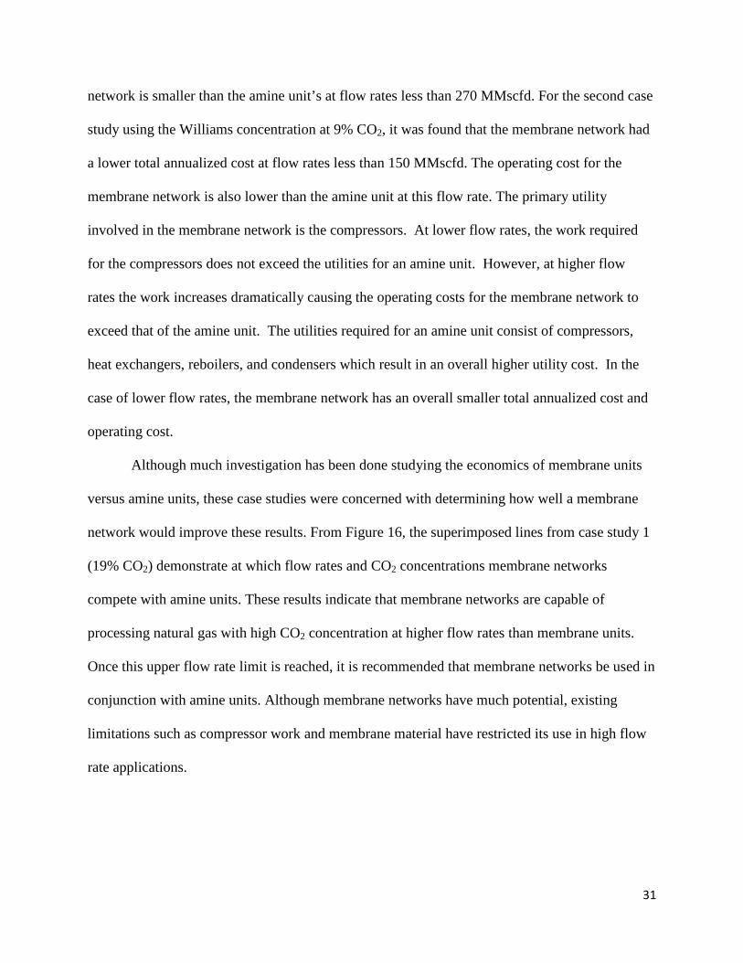
network is smaller than the amine unit’s at flow rates less than 270 MMscfd. For the second case
study using the Williams concentration at 9% CO2, it was found that the membrane network had
a lower total annualized cost at flow rates less than 150 MMscfd. The operating cost for the
membrane network is also lower than the amine unit at this flow rate. The primary utility
involved in the membrane network is the compressors. At lower flow rates, the work required
for the compressors does not exceed the utilities for an amine unit. However, at higher flow
rates the work increases dramatically causing the operating costs for the membrane network to
exceed that of the amine unit. The utilities required for an amine unit consist of compressors,
heat exchangers, reboilers, and condensers which result in an overall higher utility cost. In the
case of lower flow rates, the membrane network has an overall smaller total annualized cost and
operating cost.
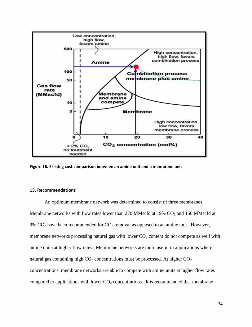
Although much investigation has been done studying the economics of membrane units
versus amine units, these case studies were concerned with determining how well a membrane
network would improve these results. From Figure 16, the superimposed lines from case study 1
(19% CO2) demonstrate at which flow rates and CO2 concentrations membrane networks
compete with amine units. These results indicate that membrane networks are capable of
processing natural gas with high CO2 concentration at higher flow rates than membrane units.
Once this upper flow rate limit is reached, it is recommended that membrane networks be used in
conjunction with amine units. Although membrane networks have much potential, existing
limitations such as compressor work and membrane material have restricted its use in high flow
rate applications.

32
Figure 14. Total annualized cost versus flow rate for an amine unit and a membrane network at 19%
CO2
$0
$10,000,000
$20,000,000
$30,000,000
$40,000,000
$50,000,000
$60,000,000
$70,000,000
$80,000,000
$90,000,000
$100,000,000
0 100 200 300 400 500 600 700To
tal A
nn
ula
ize
d C
ost
($
/yr)
15
ye
ar
pe
rio
d
Flow rate (MMscfd)
Membrane Network
Amine Unit
Flow rate (MMscfd)
FCI ($) Operating Cost ($/yr)
TAC ($/yr) 15 yr.
Membrane 2 405,000 175,000 202,000 90 31,000,000 13,000,000 15,000,000 180 61,000,000 26,000,000 30,000,000 270 92,000,000 39,000,000 45,000,000 360 123,000,000 52,000,000 60,000,000 455 153,000,000 65,000,000 75,000,000 550 184,000,000 77,000,000 90,000,000
Amine 2 632,000 490,000 532,000 90 3,700,000 21,000,000 21,000,000 180 6,600,000 30,000,000 30,000,000 270 9,200,000 37,000,000 38,000,000 360 11,500,000 43,000,000 44,000,000 455 14,000,000 49,000,000 50,000,000 550 17,000,000 54,000,000 55,000,000
Table 4. Economic analysis of an amine unit and a membrane network at 19% CO2
33
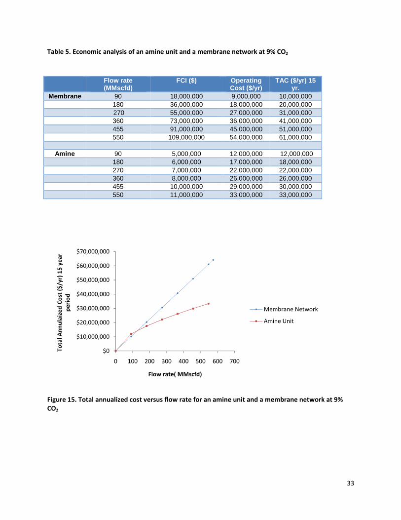
Table 5. Economic analysis of an amine unit and a membrane network at 9% CO2
Figure 15. Total annualized cost versus flow rate for an amine unit and a membrane network at 9%
CO2
$0
$10,000,000
$20,000,000
$30,000,000
$40,000,000
$50,000,000
$60,000,000
$70,000,000
0 100 200 300 400 500 600 700
To
tal A
nn
ula
ize
d C
ost
($
/yr)
15
ye
ar
pe
rio
d
Flow rate( MMscfd)
Membrane Network
Amine Unit
Flow rate (MMscfd)
FCI ($) Operating Cost ($/yr)
TAC ($/yr) 15 yr.
Membrane 90 18,000,000 9,000,000 10,000,000 180 36,000,000 18,000,000 20,000,000 270 55,000,000 27,000,000 31,000,000 360 73,000,000 36,000,000 41,000,000 455 91,000,000 45,000,000 51,000,000 550 109,000,000 54,000,000 61,000,000
Amine 90 5,000,000 12,000,000 12,000,000 180 6,000,000 17,000,000 18,000,000 270 7,000,000 22,000,000 22,000,000 360 8,000,000 26,000,000 26,000,000 455 10,000,000 29,000,000 30,000,000 550 11,000,000 33,000,000 33,000,000
34
Figure 16. Existing cost comparison between an amine unit and a membrane unit
13. Recommendations
An optimum membrane network was determined to consist of three membranes.
Membrane networks with flow rates lower than 270 MMscfd at 19% CO2 and 150 MMscfd at
9% CO2 have been recommended for CO2 removal as opposed to an amine unit. However,
membrane networks processing natural gas with lower CO2 content do not compete as well with
amine units at higher flow rates. Membrane networks are more useful in applications where
natural gas containing high CO2 concentrations must be processed. At higher CO2
concentrations, membrane networks are able to compete with amine units at higher flow rates
compared to applications with lower CO2 concentrations. It is recommended that membrane
35
networks be utilized at flow rates less than 270 MMscfd with 19% CO2. Above these flow rates,
membrane networks should be used in conjunction with an amine unit to remove CO2.
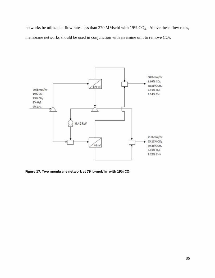
Figure 17. Two membrane network at 79 lb-mol/hr with 19% CO2
36
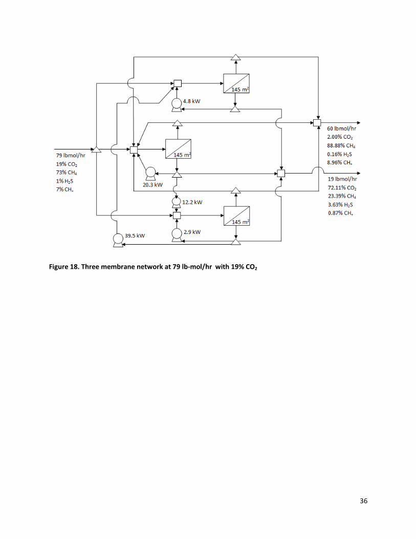
Figure 18. Three membrane network at 79 lb-mol/hr with 19% CO2
37
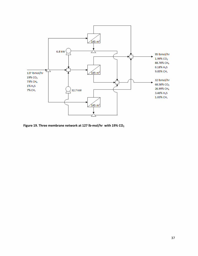
Figure 19. Three membrane network at 127 lb-mol/hr with 19% CO2
38
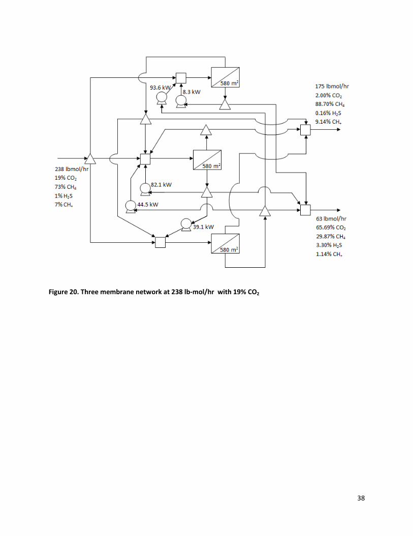
Figure 20. Three membrane network at 238 lb-mol/hr with 19% CO2

39
Figure 21. Three membrane network at 79 lb-mol/hr with 9% CO2
40
References
Baker, Richard. “Future Directions of Membrane Gas Separation Technology.” Industrial & Engineering Chemistry Research. 2002. Sarkey’s Senior Lab. 7 Feb. 2009. <http://pubs.acs.org>.
Baker, Richard. Membrane Technology and Applications (2nd Edition). Wiley. 2004.
Baker, Richard and Kaaeid Lokhandwala. “Natural Gas Processing with Membranes: An
Overview.” Industrial & Engineering Chemistry Research. 2008. Sarkey’s Senior Lab. 4 Feb. 2009 <http://pubs.acs.org>.
Dortmundt, David and Kishore Doshi. “Recent Developments in CO2 Removal Membrane Technology.” UOP LLC. 1999. Sarkey’s Senior Lab. 7 Feb. 2009. Engineering Data Book. (12th ed.). Gas Processors Supplies Association, Tulsa: 2004.
Faria, Debora C. “GAMS: Membrane Network Simulation.” School of Chemical, Biological, and Materials Engineering. January 2008.
Kookos, I.K. “A Targeting Approach to the Synthesis of Membrane Network for Gas Separations.” Membrane Science, p. 208, 193-202, 2002.
Li, N. Norman. Advanced Membrane Technology and Applications. Wiley. 2008.
Mohammadi, T., Moghadam, Tavakol, and et al. “Acid Gas Permeation Behavior Through
Poly(Ester Urethane Urea) Membrane.”Industrial & Engineering Chemistry Research. 2008. Sarkey’s Senior Lab. 4 Feb. 2009 <http://pubs.acs.org>.
Natural Gas Supply Association. 2004. Sarkey’s Senior Lab. 7 Feb. 2009. <http://www.naturalgas.org/index.asp>. Perry, R.H.; Green, D.W. (1997). Perry’s Chemical Engineers’ Handbook (7th Edition). McGraw-Hill.
Peters, Max S., Timmerhaus, Klaus D., & West, Ronald E. Plant Design and Economics for Engineers. (5th ed.). McGraw Hill, Boston: 2003.
Qi, R. and M. A. Henson, "Optimal design of spiral-wound membrane networks for gas separations.” Journal of Membrane Science, p. 75-78,1996.
Seader, J. D., and Henley, E. J. "Separation Process Principles.” New York: John Wiley & Sons, Inc., p. 718- 736, 1998.
Sridhar, S and et al. “Permeation of Carbon Dioxide and Methane Gases through Novel

41
Silver-Incorporated Thin Film Composite Pebax Membranes.” Industrial Engineering Chemistry Research 2007 Sarkey’s Senior Lab. 4 Feb 2009. <http://pubs.acs.org>
42
Appendix I
Sizing and Cost of an Amine Unit
In order to compare the equipment cost, fixed capital investment, working capital, total
capital investment and the utility cost of an amine unit versus a membrane network, a simulation
package known as Pro-II was used to develop an amine unit model. The program was able to
give us information regarding the diameter and tray spacing for each distillation column, the
overall heat transfer coefficient for each heat exchanger, pump capacity, and the heat duty for the
distillation column. Based on these results, each piece of equipment was sized according to
equipment pricing charts in Plant Design and Economics for Chemical Engineers.
Distillation Column
Once the simulation was completed, an estimated design value for the diameter and tray
spacing for each column was reported. Based on the number of trays in the column which was
chosen and the tray spacing, the height of each column can be determined. Using figure 15-11
from Plant Design and Economics for Chemical Engineers, the cost of the column can be
estimated from the vertical height and diameter of the column. Moreover, materials other than
carbon steel have adjustment factors which must be taken into consideration. However, carbon
steel was used for the external material so this adjustment was not necessary. The estimated cost
for the trays was found in figure 15-13 and is based on the column diameter as well as the type
and material of the tray. For this application, valve trays were selected using stainless steel.
Stainless steel was chosen because the trays will come into contact with an amine solution which
is extremely corrosive. Also, a quantity factor is used to adjust the cost depending on the amount
of trays used for each column.
43
Heat Exchanger & Valves
The information used to price the heat exchanger was the overall heat duty which was
reported as the product of the heat exchanger area (UA Btu/hr-F). Using table 14-5 from Plant
Design and Economics for Chemical Engineers, the overall heat transfer coefficient for each
exchanger can be estimated based on the type of component passing through the exchanger. For
example, some heat exchangers in the amine unit may contact light organics where as others
contact water. Based on the design values for the overall heat transfer coefficient, the overall
area required for the heat exchanger can be determined. From figure 14-17, the cost of the heat
exchanger can be estimated based on the total area and the material. The material used for this
application was carbon steel. The cost for the valves was found in figure 12-8 and stainless steel
gate valves were selected for this design.
Pumps
The simulation in Pro-II provided the capacity or the flow rate at the inlet of the pump which is
used to estimate the purchasing cost. From figure 12-21 in Plant Design and Economics for
Chemical Engineers, the purchasing cost for the pump can be determined based on the pump
capacity and the material used. Again carbon steel was used and a pressure adjustment factor of
1.1 was accounted for.
MDEA Calculations
In order to get an accurate equipment cost, the amount of MDEA needed for the initial start-up
was calculated. This value was determined by finding the amount of hold-up on each of the trays
in the contactor and the regenerator as well as the hold up in the pipes. Furthermore, with each
cycle some MDEA is lost and must be replenished; thus this cost was also considered.

44
Note to reader
The tables below are for three different flow rates with 19% CO2. However, flow rates ranging
from 10,000-60,000 lb-mol/hr for both 9% and 19% CO2 are detailed in an excel sheet.
Summary of Equipment and Utility Cost: 79 lb-mol/hr
Table 6. Equipment cost for an amine unit operating at 79 lb-mol/hr & 19% CO2
Columns Type No. of trays
Operating pressure Cost
1 Absorber Valve trays 6 250 psia $15,334
2 Stripper Valve trays 12 16 psia $32,736
Exchangers MOC Duty
(MMBtu/hr) Area (ft2)
1 Rich amine / Lean amine Stainless Steel 16.45 241.73955 $4,772
2 Lean amine / water Stainless Steel 10.96 37.191652 $2,651
3 Lean amine / water Stainless Steel 6.098 28.193677 $2,439
Pump MOC Power (HP)
Pump lean amine solution Stainless Steel 130 $1,803
Valve MOC Diameter (m) Type
Rich amine expansion valve Stainless Steel 0.2 Flanged $8,484
MDEA initial amt cost $552
Total $68,771
Table 7. Utility cost for an amine unit operating at 79 lb-mol/hr & 19% CO2
Cooling water
Flow(1000 kg/hr) Price ($ /m3) Cost ($ / yr)
17.53959549 0.29 $42,726
Natural gas as heating utility for reboiler
Reboiler (MMBtu/hr) Price ( $ / MMBTU)
2.73 5 $114,516
Electricity
Duty (kW) Price ($ / kWh)
4.42 0.062 $2,301.94
MDEA Recycle
Flow (lb/hr) Price ($/lb)
0.11917 1.54 $1,541.58
Total $161,086
45
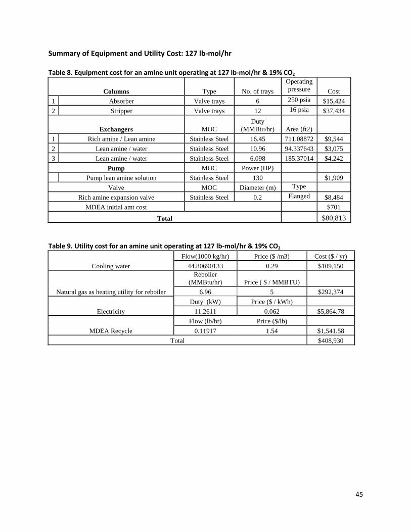
Summary of Equipment and Utility Cost: 127 lb-mol/hr
Table 8. Equipment cost for an amine unit operating at 127 lb-mol/hr & 19% CO2
Columns Type No. of trays
Operating pressure Cost
1 Absorber Valve trays 6 250 psia $15,424
2 Stripper Valve trays 12 16 psia $37,434
Exchangers MOC Duty
(MMBtu/hr) Area (ft2)
1 Rich amine / Lean amine Stainless Steel 16.45 711.08872 $9,544
2 Lean amine / water Stainless Steel 10.96 94.337643 $3,075
3 Lean amine / water Stainless Steel 6.098 185.37014 $4,242
Pump MOC Power (HP)
Pump lean amine solution Stainless Steel 130 $1,909
Valve MOC Diameter (m) Type
Rich amine expansion valve Stainless Steel 0.2 Flanged $8,484
MDEA initial amt cost $701
Total $80,813
Table 9. Utility cost for an amine unit operating at 127 lb-mol/hr & 19% CO2
Cooling water
Flow(1000 kg/hr) Price ($ /m3) Cost ($ / yr)
44.80690133 0.29 $109,150
Natural gas as heating utility for reboiler
Reboiler (MMBtu/hr) Price ( $ / MMBTU)
6.96 5 $292,374
Electricity
Duty (kW) Price ($ / kWh)
11.2611 0.062 $5,864.78
MDEA Recycle
Flow (lb/hr) Price ($/lb)
0.11917 1.54 $1,541.58
Total $408,930

46
Summary of Equipment and Utility Cost: 238 lb-mol/hr & 19% CO2
Table 10. Equipment cost for an amine unit operating at 238 lb-mol/hr & 19% CO2
Columns Type No. of trays
Operating pressure Cost
1 Absorber Valve trays 6 250 psia $27,932
2 Stripper Valve trays 12 16 psia $53,235
Exchangers MOC Duty
(MMBtu/hr) Area (ft2)
1 Rich amine / Lean amine Stainless Steel 16.45 804.06735 $15,907
2 Lean amine / water Stainless Steel 10.96 113.88082 $4,242
3 Lean amine / water Stainless Steel 6.098 86.315086 $3,712
Pump MOC Power (HP)
Pump lean amine solution Stainless Steel 130 $2,651
Valve MOC Diameter (m) Type
Rich amine expansion valve Stainless Steel 0.2 Flanged $8,484
MDEA initial amt cost $871
Total $117,033
Table 11. Utility cost for an amine unit operating at 238 lb-mol/hr & 19% CO2
Cooling water
Flow(1000 kg/hr) Price ($ /m3) Cost ($ / yr)
53.48166714 0.29 $130,281
Natural gas as heating utility for reboiler
Reboiler (MMBtu/hr) Price ( $ / MMBTU)
8.311611536 5 $349,088
Electricity
Duty (kW) Price ($ / kWh)
13.62 0.062 $7,093.30
MDEA Recycle
Flow (lb/hr) Price ($/lb)
0.23834 1.54 $3,083.17
Total $489,545

47
Pro-II Verification
A Pro-II simulation was performed for all resulting membrane networks. This was done
in order to verify the compressor work as it is a major contributing factor in the total cost. The
Pro-II simulation for the 3 membrane network at 238 lb-mol/hr is shown in the following figure.
Figure 22. Membrane network simulation
The following table is a comparison of the compressor work found from our model and Pro-II.
Table 12. Compressor work comparison
48
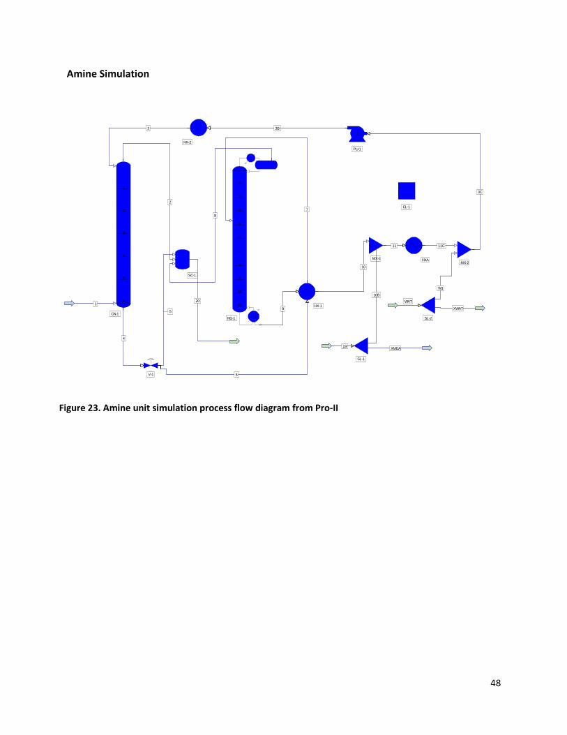
Amine Simulation
1
2
3
4
5
6
CN-1
V-1
HX-1
2
3
4
5
6
7
8
9
10
11
1
12RG-1
CL-1
SL-2
SC-1
SL-1
MX-1 HXAMX-2
PU-1
HX-2
3
1
2
4
5
6
9
10
7
8
WAT
W1
XWAT
20
19
10B
XMEA
11 11C
3C
3B
Figure 23. Amine unit simulation process flow diagram from Pro-II
49
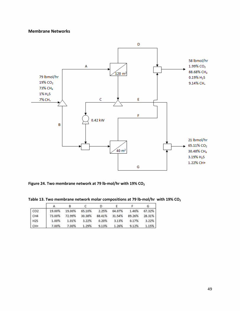
Membrane Networks
Figure 24. Two membrane network at 79 lb-mol/hr with 19% CO2
Table 13. Two membrane network molar compositions at 79 lb-mol/hr with 19% CO2

50
Figure 25. Three membrane network at 79 lb-mol/hr with 19% CO2
Table 14. Three membrane network molar compositions at 79 lb-mol/hr with 19% CO2

51
Figure 26. Three membrane network at 127 lb-mol/hr with 19% CO2
Table 15. Three membrane network molar compositions at 127 lb-mol/hr with 19% CO2
52
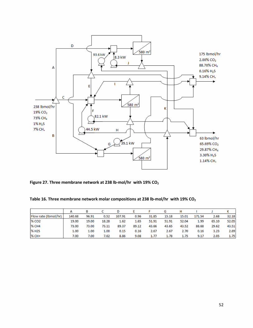
Figure 27. Three membrane network at 238 lb-mol/hr with 19% CO2
Table 16. Three membrane network molar compositions at 238 lb-mol/hr with 19% CO2

53
Figure 28. Three membrane network at 79 lb-mol/hr with 9% CO2
Table 17. Three membrane network molar compositions at 79 lb-mol/hr with 9% CO2