Use of Linear Discriminant Analysis in Song Classification

University of Mississippi University of Mississippi

eGrove eGrove

Honors Theses Honors College (Sally McDonnell Barksdale Honors College)

Spring 5-1-2021

Use of Linear Discriminant Analysis in Song Classification: Use of Linear Discriminant Analysis in Song Classification:

Modeling Based on Wilco Albums Modeling Based on Wilco Albums

Caroline Pollard

Follow this and additional works at: https://egrove.olemiss.edu/hon_thesis

Part of the Applied Statistics Commons, Categorical Data Analysis Commons, and the Statistical

Models Commons

Recommended Citation Recommended Citation Pollard, Caroline, "Use of Linear Discriminant Analysis in Song Classification: Modeling Based on Wilco Albums" (2021). Honors Theses. 1909. https://egrove.olemiss.edu/hon_thesis/1909

This Undergraduate Thesis is brought to you for free and open access by the Honors College (Sally McDonnell Barksdale Honors College) at eGrove. It has been accepted for inclusion in Honors Theses by an authorized administrator of eGrove. For more information, please contact [email protected].

https://egrove.olemiss.edu/

https://egrove.olemiss.edu/hon_thesis

https://egrove.olemiss.edu/honors

https://egrove.olemiss.edu/honors

https://egrove.olemiss.edu/hon_thesis?utm_source=egrove.olemiss.edu%2Fhon_thesis%2F1909&utm_medium=PDF&utm_campaign=PDFCoverPages

http://network.bepress.com/hgg/discipline/209?utm_source=egrove.olemiss.edu%2Fhon_thesis%2F1909&utm_medium=PDF&utm_campaign=PDFCoverPages




https://egrove.olemiss.edu/hon_thesis/1909?utm_source=egrove.olemiss.edu%2Fhon_thesis%2F1909&utm_medium=PDF&utm_campaign=PDFCoverPages

mailto:[email protected]

USE OF LINEAR DISCRIMINANT ANALYSIS IN SONG CLASSIFICATION: MODELING

BASED ON WILCO ALBUMS

By

Caroline Pollard

A thesis submitted to the faculty of The University of Mississippi in partial fulfillment of the

requirements of the Sally McDonnell Barksdale Honors College.

Oxford, MS

May 2021

Approved By

______________________________

Advisor: Professor John Latartara

______________________________

Reader: Professor Gerard Buskes

______________________________

Reader: Professor Michael Worthy

© 2021

Caroline Pollard

ALL RIGHTS RESERVED

ACKNOWLEDGEMENTS

I would like to extend a big thank-you to my readers, Dr. Buskes and Dr. Worthy, and

especially my advisor, Dr. Latartara. It has such a pleasure working under and with these

knowledgeable professors. They have kindly offered guidance and critiques through this process,

and my argument and writing would not be as strong without their work on this as well. It is truly

valuable to learn from those much wiser.

ABSTRACT

CAROLINE POLLARD: Use of Linear Discriminant Analysis in Song Classification (Under the

direction of John Latartara)

The study of music recommender algorithms is a relatively new area of study. Although

these algorithms serve a variety of functions, they primarily help advertise and suggest music to

users on music streaming services. This thesis explores the use of linear discriminant analysis in

music categorization for the purpose of serving as a cheaper and simpler content-based

recommender algorithm. The use of linear discriminant analysis was tested by creating linear

discriminant functions that classify Wilco’s songs into their respective albums, specifically A.M.,

Yankee Hotel Foxtrot, and Sky Blue Sky. 4 sample songs were chosen from each album, and song

data was collected from these samples to create the model. These models were tested for

accuracy by testing the other, non-sample, songs from the albums. After testing these models, all

proved to have an accuracy rate of over 80%. Not being able to write computer code for this

algorithm was a limiting factor for testing applicability on a larger-scale, but the small-scale

model proves to classify accurately. I predict this accuracy to hold on a larger-scale because it

was tested on very similar music when in reality, these models work to classify a diverse range

of music.

1

TABLE OF CONTENTS

List of Figures……………………………………………………………………………………..2

Introduction………………………………………………………………………………………..4

Chapter 1: Literature Review……………………………………………………………………...7

Chapter 2: Methodology…………………………………………………………………………19

Chapter 3: Analysis……………………………………………………………………………....23

Chapter 4: Discussion and Conclusion…………………………………………………………..66

Bibliography……………………………………………………………………………………..70

2

LIST OF FIGURES

Figure 1 ....................................................................................................................................................... 12 Figure 2 ....................................................................................................................................................... 12 Figure 3 ....................................................................................................................................................... 14 Figure 4 ....................................................................................................................................................... 22 Figure 5 ....................................................................................................................................................... 24 Figure 6 ....................................................................................................................................................... 25 Figure 7 ....................................................................................................................................................... 27 Figure 8 ....................................................................................................................................................... 27 Figure 9 ....................................................................................................................................................... 27 Figure 10 ..................................................................................................................................................... 28 Figure 11 ..................................................................................................................................................... 28 Figure 12 ..................................................................................................................................................... 28 Figure 13 ..................................................................................................................................................... 29 Figure 14 ..................................................................................................................................................... 30 Figure 15 ..................................................................................................................................................... 31 Figure 16 ..................................................................................................................................................... 31 Figure 17 ..................................................................................................................................................... 31 Figure 18 ..................................................................................................................................................... 32 Figure 19 ..................................................................................................................................................... 32 Figure 20 ..................................................................................................................................................... 32 Figure 21 ..................................................................................................................................................... 33 Figure 22 ..................................................................................................................................................... 33 Figure 23 ..................................................................................................................................................... 33 Figure 24 ..................................................................................................................................................... 34 Figure 25 ..................................................................................................................................................... 34 Figure 26 ..................................................................................................................................................... 34 Figure 27 ..................................................................................................................................................... 35 Figure 28 ..................................................................................................................................................... 35 Figure 29 ..................................................................................................................................................... 35 Figure 30 ..................................................................................................................................................... 38 Figure 31 ..................................................................................................................................................... 38 Figure 32 ..................................................................................................................................................... 39 Figure 33 ..................................................................................................................................................... 39 Figure 34 ..................................................................................................................................................... 40 Figure 35 ..................................................................................................................................................... 40 Figure 36 ..................................................................................................................................................... 41 Figure 37 ..................................................................................................................................................... 42 Figure 38 ..................................................................................................................................................... 48 Figure 39 ..................................................................................................................................................... 49 Figure 40 ..................................................................................................................................................... 50 Figure 41 ..................................................................................................................................................... 50

3

Figure 42 ..................................................................................................................................................... 51 Figure 43 ..................................................................................................................................................... 52 Figure 44 ..................................................................................................................................................... 52 Figure 45 ..................................................................................................................................................... 52 Figure 46 ..................................................................................................................................................... 56 Figure 47 ..................................................................................................................................................... 56 Figure 48 ..................................................................................................................................................... 57 Figure 49 ..................................................................................................................................................... 57 Figure 50 ..................................................................................................................................................... 58 Figure 51 ..................................................................................................................................................... 59 Figure 52 ..................................................................................................................................................... 59 Figure 53 ..................................................................................................................................................... 59 Figure 54 ..................................................................................................................................................... 63 Figure 55 ..................................................................................................................................................... 63 Figure 56 ..................................................................................................................................................... 64 Figure 57 ..................................................................................................................................................... 64 Figure 58 ..................................................................................................................................................... 65

4

Introduction

Simply listening to a piece of music, the human brain is quick to sort and tag it with a

description. This occurs without a listener even knowing what is behind that or what defines the

categories in the brain that operate like sound organization bins. This categorization may be

based on genre, artist, time period or general mood, just to name a few possibilities, but what

each of these categories has in common is that they are defined by sound, though the definition

of that sound may vary.

Through both qualitative and quantitative studies of music many analysts have sought to

give definition and boundaries to these categories. With definition, the categories become useful

in studying, organizing, and consuming music. Many arguments exist concerning the

categorization of music based on elements ranging from instrumentation to lyrical analysis to

harmonic analysis.

This thesis is not meant to create a new musical category definition or critique existing

classification systems; rather, this work explores a mathematical technique known as linear

discriminant analysis to categorize “popular” music based on a combination of harmonic,

instrumentation, structural, and waveform data. A blend of these elements provides a more

inclusive way of categorizing music and considers both the layers of the raw content of the piece

and the production elements. Furthermore, the mathematical nature of the classification could

5

allow for further development and implementation in AI music platforms to create a more

holistic content-based music classification.

I argue linear discriminant analysis can be used to easily compare and contrast musical

genre in popular music, including both sonic as well as cultural elements. Rather than trying to

prove linear discriminant analysis can define musical categories or suggest this method is the

most accurate for music classification, my goal is to show that linear discriminant analysis can be

trained to reach similar accuracy levels as the algorithms used by iTunes and Spotify. Songs

drawn from Wilco’s albums, A.M., Yankee Hotel Foxtrot, and Sky Blue Sky, are used as my test

case from which I collect my data. Linear discriminant analysis is a method of statistical

classification that finds linear boundaries between 2 or more classes based on variation within

and between data sets of the separate classes. It is a popular model to use for prediction in

classifying an object of an unknown class or even predicting future outcomes. For example, in

healthcare, linear discriminant analysis is often used to determine the likelihood of health-risk

factors leading to certain diseases or health complications. Compared to other statistical

classification methods, linear discriminant analysis is often easier to interpret, and is less

expensive and space consuming to run computationally a large scale.

In this thesis, I will test my modeling technique on a small-scale by constructing three

separate algorithms that can categorize Wilco songs into their correct albums. Wilco, into their

correct albums. If testing this technique on music from the same band shows high accuracy, it

will most likely have success in distinguishing music that is more different. These algorithms are

based on three different Wilco albums, A.M., Yankee Hotel Foxtrot, and Sky Blue Sky and each

algorithm compares a pair of these albums. I collected data from 12 songs, chosen at random,

which includes 4 from each album. This data was used to train, or create, my algorithms, and

6

after the algorithms were trained, I tested them for accuracy by applying the remainder of the

songs from the albums.

While holistic modeling techniques exist, they are often so complicated and require so

much storage that they become excessively expensive to create and run. Larger corporations like

iTunes and Spotify are among the few that can maintain highly accurate music classification

algorithms. Creating a linear discriminant analysis model based on the same range of data would

open the door for an easier and less expensive technique that is still accurate. Ultimately, a model

like this would help grow and strengthen Music Information Retrieval systems as well as smaller

business that cannot afford the more expensive algorithms.

7

Chapter 1: Literature Review

Music Categorization

To begin this study, it is important to note the different ways others have attempted to

categorize music and their use of diverse methodologies. The most popular categorical analysis

of music is of genre, so the majority of this literature review will trace the different

methodologies used for defining genre. The following studies specifically examine rock and

popular musical genres, since this is the focus of my research. Nolan Foxworth (2017) gives a

framework for identifying musical genres through harmonic analysis. By specifically studying

tonality of chords in Rock R&B/Hip-Hop and Christian music, Foxworth creates his own “rules”

for each genre and then descriptively proves why songs of these genres fit his established

“rules.” For example, he notes that Rock music typically tonicizes the vi to create a minor feel

without actually entering the minor key and uses this as one of his “rules” of rock music.

Categorization through Harmonic Analysis is not unique to Foxworth’s study. Various methods

of harmonic analysis exist within the realm of genre categorization. Abeber, Brauer, and

Lukashevich (2012) studied bass line and the way it relates to genre. The bass line stands out to

many listeners of music and can be a way listeners distinguish sounds by ear. By studying the

pitches and rhythm of base lines, Abeber, Brauer, and Lukashevich presented bass line patterns

that lead to differing harmonic progressions that they argue define genres.

8

Brad Osborn (2013) analyzed structure and form in rock music after 1990, creating and

defining a type called “terminally climactic forms.” These forms are defined by their balance

between an expected highpoint in a song (usually the chorus Osborn describes) and the

“thematically independent terminal climax.” He then defines three subforms and analytically

supports these subforms by categorizing rock music into these forms. This is an example of rock

music categorized by its formal sections.

In a more statistical sense, Glickman, Brown, and Song (2019) create an authorship

algorithm to distinguish between Beatles songs composed by Lennon and McCartney. This

algorithm is based off of a combination of harmonic and melodic analysis of all known Lennon

or McCartney songs. Glickman, Brown, and Song focused specifically on the occurrence of

melodic notes, chords, melodic note pairs, chord change pairs, and four-note melody contours

and created variables from sub categories of these categories listed. This analysis screened for

differentiating variables between the two artists and then implemented the statistically significant

variables into a prediction model created with logistic regression and elastic net regularization.

When tested on songs of known authorship, the model proved to have a 76% classification

accuracy. This method combines both harmonic and melodic features to sort music.

To classify between early and late punk music, Chris Kemp (2004) carried out both a

qualitative and quantitative investigation of the two periods. This hybrid technique attempts to

attain a holistic view of what factors differentiate the early and late period. By conducting focus

groups, interviews, and surveys, Kemp collected data. In his quantitative study, Kemp does not

focus on one specific aspect of the music. Instead, he looks at a variety of elements such as the

number of lines in the verses compared to the chorus and deviation of pitch. By using a two-

tailed t-test, he starts with a wide range of variables and funnels the list down to what will

9

actually be useful in differentiating the periods of punk music. This test is a statistical method of

determining the difference between the means of the same variable in two different populations.

It can give numerical detail and description to how different two populations are. Kemp then

applies the statistically significant variables for use in Bayesian analysis to make a prediction

model for punk songs.

This overview does not cover, by any means, the full spectrum of music categorization

efforts, but rather highlights the variety in which individuals have studied this topic. With the

exception of Osborn’s study of form, each of these studies took previously defined taxonomy

systems such as genre, style, or artist and sought to further explore their meanings.

Methods of Statistical Classification

While qualitative and quantitative methods of describing music can be equally effective

descriptors, music described quantitatively can enter a whole new realm of possibilities. The

primary reason music is grouped by quantitative methods today is for music information retrieval

(MIR), a newly emerging science of retrieving information from music. By combining

mathematical algorithms with machine learning, MIR makes it so that music can be analyzed,

sorted, and searched on a large scale. This information can create the basis for music

recommender systems, separate layers in audio (this is what creates karaoke tracks), and

categorize music by genre, mood, and artist among other things.

The mathematical algorithms mentioned above are all types of statistical classification

algorithms. In statistics, classification is the process of using observations of known classes to

identify where a new observation, of unknown class, belongs. For example, this is the way

emails are often categorized as spam or non-spam. Medically, an example of statistical

10

classification could be diagnosing a patient of a disease based on symptoms like blood pressure

level, pulse rate, and body temperature. Beyond just categorization, this type of statistics is used

in decision-making probability. Data taken from known categories is called prediction data, and

this data helps construct various types of mathematical models for prediction through a process

called learning or training. These models help draw boundaries in data.

Mathematical prediction models fall into one of two categories: parametric and non-

parametric. Parametric models rely on assumptions to simplify the learning process. By

assuming the functional form of a line (or any type of boundary), these algorithms learn quickly

and produce easy-to-understand results. Parametric functions, however, are limited in the sense

that they do not allow for much flexibility in the shape of the boundary. This can lead to limits in

finding best fit boundaries for data with high variance. On the other hand, non-parametric models

do not rely at all on assumptions and function much more flexibly. Because they do not rely on

assumptions, they are not models that can simply be created by hand. Non-parametric models are

highly complex and constantly changing via artificial intelligence to give unique best-fit data.

They are trained much more slowly and require large amounts of data to function. Because this

study focuses on a type of parametric classification, I will narrow my discussion down to that

research.

The most basic forms of parametric classification is linear regression. Linear regression

models represent a prediction of the relationship between an explanatory and response variable.

The form of this model is a known function, y=ax+b.

One of the most common and recently studied parametric classification methods is Naive

Bayes classifier. Naive Bayes classifier is actually a broad term for models based on Bayes

Theorem, so there are several variations. Bayes Theorem calculates probability of one event

11

occurring based on the occurrence of another event (see section below for mathematical details

of this theorem). This method, compared to the others to be discussed, is optimal in minimizing

the probability of error. In order to use this method, though, conditional probability density

functions must be known for each class. While difficult to obtain on a larger scale and requiring

extended time and large storage when implemented properly, however, this classifier method

exceeds the performance of all other types of classification methods.

The second large category of parametric classification methods is discriminant analysis.

This method is older and simpler compared to Naive Bayes and assumes the variables follow a

multivariate normal distribution (mathematically explained below). Essentially, this assumes the

variables are all quantitative and continuous. Despite its simplicity, discriminant analysis is often

the first to be used in tackling real-world problems due to its easy-to-interpret nature. In

discriminant analysis, we create a discriminant function that tells us how likely a piece of data

comes from a certain class.

This function look like:

Here, 𝜋𝑖 is the prior probability of the class Fi and x is the piece of data we want to classify. The

x where these two functions have the same value is where the boundary lies. Discriminant

analysis primarily falls under two categories: linear and quadratic.

These two types of discriminant analysis follow the function above but in slightly

different ways. Linear discriminant analysis assumes that the covariance matrices of the two

classes are equal or close to equal. In this case, the boundary is a line dividing two classes.

Figure 1 graphically shows this linear division:

12

And the discriminant function becomes:

This function, though seemingly very different from the discriminant analysis function

mentioned, holds the same basic components but is a linear function in x.

Quadratic discriminant analysis is useful when covariance matrices of a data set are not

equal or near equal. When this occurs, the matrices do not cancel out and instead result in a

quadratic function dividing the classes. Figure 2 graphically shows this:

Figure 2

Figure 1

13

The quadratic discriminant function is shown below:

Neither is arguably more useful than the other. While quadratic discriminant analysis proves

more flexible, linear discriminant analysis is able to maximize space better between classes due

to stronger data correlation. They must just be used for different instances.

Linear Discriminant Analysis

Because of its simplicity and clarity compared to other statistical classification methods,

linear discriminant analysis (LDA) has been used for many real-world applications. A well-

known use of this model can be NYU professor Edward Altman’s (1968) bankruptcy model that

can predict the probability of company bankruptcy with 80-90% accuracy. He bases his model

on five known company characteristics that exist in failing and bankrupt companies. This model

classifies companies into two groups: bankruptcy and non-bankruptcy. Frederick Mosteler and

David Wallace (1963) use LDA to predict authorship of The Federalist Papers between

Hamilton and Madison. By using word counts as their variables of discrimination, Mosteler and

Wallace concluded that Madison rather than Hamilton wrote the papers. Linear discriminant

analysis has also been used in text-genre identification. Jussi Karlgren and Douglass Cutting

found “practical promise” in their application of LDA to identifying between fiction and non-

fiction texts. LDA has been used beyond these examples for real-world classification problems,

but this specific method has yet to be used in music classification.

To understand Linear Discriminant Analysis the Gaussian Distribution must be

understood first. Gaussian distribution, commonly referred to as normal distribution, is one of the

14

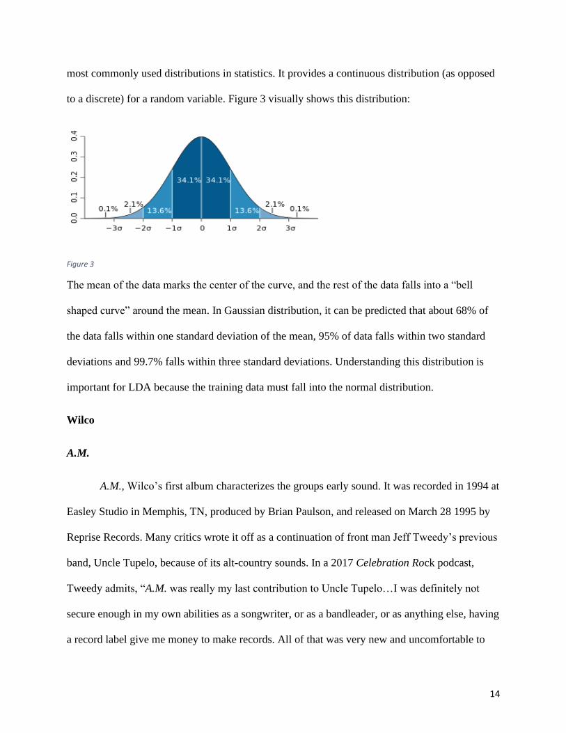
most commonly used distributions in statistics. It provides a continuous distribution (as opposed

to a discrete) for a random variable. Figure 3 visually shows this distribution:

Figure 3

The mean of the data marks the center of the curve, and the rest of the data falls into a “bell

shaped curve” around the mean. In Gaussian distribution, it can be predicted that about 68% of

the data falls within one standard deviation of the mean, 95% of data falls within two standard

deviations and 99.7% falls within three standard deviations. Understanding this distribution is

important for LDA because the training data must fall into the normal distribution.

Wilco

A.M.

A.M., Wilco’s first album characterizes the groups early sound. It was recorded in 1994 at

Easley Studio in Memphis, TN, produced by Brian Paulson, and released on March 28 1995 by

Reprise Records. Many critics wrote it off as a continuation of front man Jeff Tweedy’s previous

band, Uncle Tupelo, because of its alt-country sounds. In a 2017 Celebration Rock podcast,

Tweedy admits, “A.M. was really my last contribution to Uncle Tupelo…I was definitely not

secure enough in my own abilities as a songwriter, or as a bandleader, or as anything else, having

a record label give me money to make records. All of that was very new and uncomfortable to

15

me, and so the comfortable reaction to that was to try and hang on to the Uncle Tupelo fans.”

Wilco nearly kept all members of Uncle Tupelo, except front-man, Jay Farrar. Brian Paulson is a

musician, record producer, and audio engineer who is also known for recording albums by Uncle

Tupelo, Son Volt, and Slint.

Yankee Hotel Foxtrot

Yankee Hotel Foxtrot was recorded late 2000/early 2001. When the album was rejected

by their label (Reprise Records), the band was given the rights to the album and decided to

record and produce it in their very own Chicago loft. In 2002, Wilco sold the album to Nonesuch

Records, and to this day many consider this Wilco’s breakthrough album. Yankee Hotel Foxtrot

was officially released in April of 2002 (although it had been released on Wilco’s website for a

few months), and it received overwhelmingly positive reviews from critics and even reached #13

on the Billboard 200. In short, Yankee Hotel Foxtrot was the band’s most successful release at

the time, and still one of their most successful today.

This album was made during a period of change for the band. In Wilco’s 1999 album,

Summerteeth, they transitioned away from their country sound heard in A.M. and began

experimenting with influence from 60s pop. Yankee Hotel Foxtrot marks the pinnacle of this

experimentation and change as heard through the various instruments used and its unique

production, by Jim O’Rourke. Indeed, this change in sound created friction within the band,

resulting in a transition of band members to accompany the change Jeff Tweedy envisioned.

Between A.M. and Yankee Hotel Foxtrot, Wilco lost Max Johnston and Brian Henneman,

and in the process of creating Yankee Hotel Foxtrot, Glenn Kotche replaced Ken Coomer as the

drummer (heavy metal drummer!). Glen Kotche was not the only new addition between albums,

16

though, the band gained four more members: Jay Bennett, Craig Christiansen, Jessy Greene and

Leroy Bach. This would mark Jay Bennett’s final album with Wilco, though, after a falling-out

with the band in this period of change.

A year before the making of Yankee Hotel Foxtrot, Jeff Tweedy heavily immersed

himself in Jim O’Rourke’s music- particularly his 1997 solo album “Bad Timing.” In an

interview, Tweedy states, “It [O’Rourke’s music] ended up blowing my mind more than just

about any record I’d heard in the last five years. The patience of the arrangements really

appealed to me, the idea that it’s not about how fast you get from point A to point B, but

savoring every second of the journey.” Jim O’Rourke is known for his “obscure, avant-garde

projects” (“Jim O’Rourke Mixes Wilco Controversy”). Tweedy, O’Rourke, and Kotche met and

instantly began writing songs together in a project called “Loose Fur.” Some consider this an

outline of Yankee Hotel Foxtrot because following its creation, Tweedy knew he wanted Wilco

to head in the direction of its “inventive drumming, skewed guitars and shape-shifting

arrangements that bridge pop and noise rock” (“Jim O’Rourke Mixes Wilco Controversy”). In an

interview with the Chicago Tribune, O’Rourke says, “’The second Jeff asked me to mix the

record, I said to him ‘I will get you dropped [from your record label] and when they really did

get dropped, I was terrified that he would never talk to me again” Contrary to popular belief,

O’Rourke actually mixed the album by stripping about 80% of the noise layers to bring out the

music’s underlying sounds.

Sky Blue Sky

Sky Blue Sky is known by many to be one of Wilco’s most divisive albums. Following the

release of Yankee Hotel Foxtrot and A Ghost Is Born, two very experimental records, Wilco

recedes in a sense to a laid-back soft-rock sound in Sky Blue Sky. Despite its divisiveness, it

17

climbed to #4 on the billboards because of hits like “Impossible Germany and “You Are My

Face.” (my book) In Pitchfork’s official review of the album, Rob Mitchum writes, “Among Sky

Blue Sky’s most distressing attributes is its misuse of the experimentalist weapons at Tweedy’s

command: drummer Glenn Kotche is given no room to stretch beyond routine time-keeping, and

cline is used for his capacity to rip and wail rather than his ear for texture and atmosphere,”

noting the ways in which Sky Blue Sky lacks in experimentation. Drum beats are more consistent

and carry less of the melody, and the guitars do the same with the exception of Cline’s solos.

Between Yankee Hotel Foxtrot and Sky Blue Sky, the band lost members Jay Bennett and

Leroy Bach but added Mikael Jorgensen (piano), Pat Sansone (multi-instrumentalist), and Nels

Cline (guitar). “But after A Ghost is Born was released in 2004, the band’s volatile internal

chemistry stabilized. The current incarnation of Wilco is also the longest lived, at a mere three

years. Sky Blue Sky is as much a testament to that stability as anything else: ‘the silver lining of

all those changes is that the DNA of the band keeps changing’ Sirratt says, ‘and so none of the

albums really sound alike.’” (“Back to The Basics: An Interview With Wilco”). Major changes

occurred in Tweedy’s life between Yankee Hotel Foxtrot and Sky Blue Sky. In 2004, he entered a

rehab clinic for drug dependency, depression, and anxiety. He even quit smoking, and came out

healthier than he had been for the previous decade. Tweedy attributes his cleaner vocals, better

band collaboration, and focus on Sky Blue Sky greatly to his improved health (“Back to The

Basics: An Interview With Wilco”).

The addition of Nels Cline in this period is arguably one of the most transformative

elements between albums. Before joining Wilco, Cline appeared on several albums and even had

his own bands like The Nels Cline Singers, The Nels Cline Trio, and The Nels Cline Quartet.

Cline primarily played jazz in these projects. Cline told Diffuser’s Chris Kissell in 2014, “‘We

18

were on tour in 1996, opening for Golden Smog, and the Fibbers loved Jeff. Later, after the

Fibbers had broken up, Carla Bozulich on a solo project, we opened for Wilco. We were playing

Chicago, and all the guys from the band came and checked us out. I met everyone in the band,

and then Leroy Bach left, and … Jeff wanted some random element that was going to take the

music somewhere less familiar.’”

19

Chapter 2: Methodology

Listening

I began my process by listening. Distinguishing by sound. What songs sound different? The

same? And in a broader context, what albums? I listened for change over time in Wilco’s music

and divided it into “eras.” Over time, I noticed the music almost jump genres. From alt-country,

to rock, to soft rock/folkish, to more mellow folk. I could hear differences but then the next step

was to figure out precisely the “why” and “what” of those differences. My next step was to

research and look for causes of change over time. Using the existing knowledge I have about

music, I brainstormed a few elements I knew would cause a musician’s music to change over

time. I researched the history of the band, the members individually, the albums, and the

production. To narrow my search, I chose 3 albums, one from each Wilco era to study the band’s

change over time.

Variable Observation

I began looking at these elements as variables that could inflict change on the band’s music.

This process of observation allowed me to narrow my search for variables a great deal instead of

going in blind. Because of my limited time and resources (working by hand), I knew I would

have to be strategic and intentional in my search for distinguishing variables. Ideally, this would

not be a part of methodology if these modeling techniques were used on a larger scale and with

computers, hundreds of variables could be extracted and tested for significance in a matter of

seconds. The two most significant changes I saw over time for the band was the structure of the

20

band itself and difference in production on their albums. From here, I tracked these variables

hoping to narrow my search.

Sample Selection and Data Collection

I then turned my observations of certain variables into numerical data. To do this, four songs

from each album were chosen at random in order to extract data. These songs were selected by a

random number generator to help eliminate biases in my research. From these songs, I collected

harmonic data, song structure data, and sonic data.

Variable Elimination

The next step was to narrow down the variables that would show empirical, statistical

difference between the albums. In the end, this will give the most accurate results and ensure that

the mathematical model output is not occurring simply by chance. A standard way to determine

this significance is through performing a two-tailed t-test. Specifically, I chose to use the

Student’s Two Tail t-Test because this type of test is specific to small sample sizes. Essentially,

this test determines the difference between two sample means and qualifies the data difference as

either not significant, slightly significant, significant, or very significant. In this study, only

variables deemed significant or very significant by this test were used. Because I found no

variables that proved to be significant or very significant between all 3 of the albums in this step,

I opted to create 3 different models. Each model compares the albums in pairs (i.e. model for

album 1 vs. album 2, a model for album 1 vs. album 3, a model for album 2 vs. album 3).

Creating Models With LDA

Each model was created using 3 variables that tested to be significant or very significant in

the variable elimination step, and this data is called the “training data” because it is the data that

creates the model. Each model consists of two discriminant functions. For example, the model

21

comparing album 1 to album 2 has a function based on covariance data, data between the two

albums, and data from album 1 called F1. The second function in this model is based on the same

covariance data and data from album 2 called F2. When the training data is plugged back into

functions, each outputs a numerical value, and the two values can be graphed as a point (F1, F2)

on a 2-dimensional plane. The collection of these points is then used to find a line-of-best-fit,

sometimes known as a regression line. This line is the linear barrier between the two classes.

Model Testing

To test the model, accuracy can be tested by calculating the F1 and F2 values of songs of

known albums (this is the test data) and graphing them along the regression line. Visually, the

accuracy should be apparent based on which side of the line the data point falls on. Some points

may lie close to or directly on top of the line, and in this case, classification can be verified by

plugging the F1 value into the regression equation. Since the regression model is only a

prediction model, the output will be a predicted F2 value. Comparing the predicted F2 value (the

actual point on the line) to the real F2 value will show whether the point lies above or below the

line. Each song was either classified as accurate or not accurate, and total model accuracy was

found by dividing the number of accurate classifications by the total number of test songs. In this

thesis, I classified a model as accurate if the test data shows an accuracy of 80% or higher.

22

Chapter 3: Analysis

Variable Collection

My data was collected from a sample of four songs from the three albums: A.M., Yankee

Hotel Foxtrot, and Sky Blue Sky. I assigned a number to each song in each album, and album-by-

album used a random number generator to randomly select four songs. Figure 4 displays my

samples:

A.M. Yankee Hotel Foxtrot Sky Blue Sky

That's Not the Issue Heavy Metal Drummer Sky Blue Sky

It's Just That Simple War on War Hate it Here

Casino Queen I Am Trying to Break Your Heart You Are My Face

Box Full of Letters Pot Kettle Black Impossible Germany

Figure 4

Using these songs, I collected large amounts of data, ranging from harmonic data to

lyrical data. In this part of the process, I primarily looked for data consistency within each album

since it indicates the absence of randomness to the variable.

Instrument Data

The first data set I tracked across the three albums was the instrument data. I examined

change in types of instruments, change in band members that cause stylistic change to

23

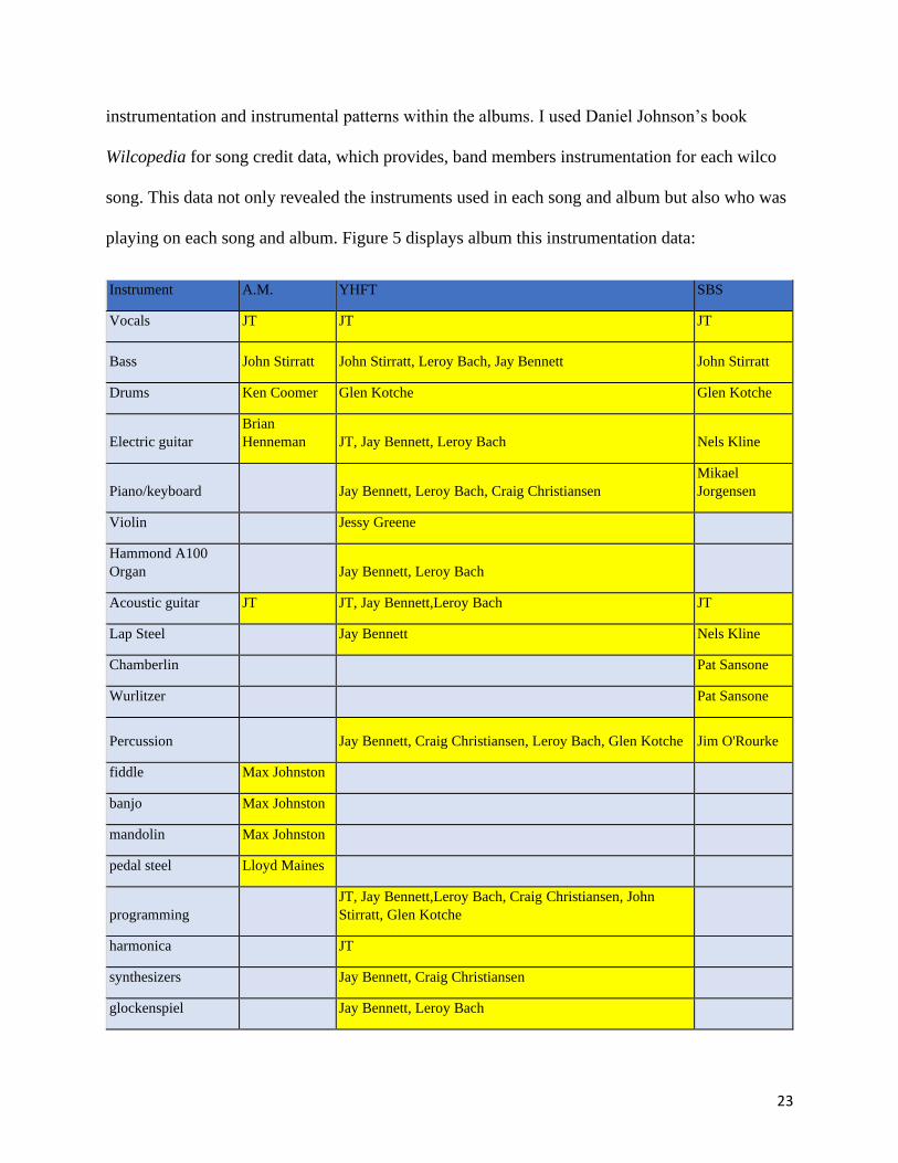
instrumentation and instrumental patterns within the albums. I used Daniel Johnson’s book

Wilcopedia for song credit data, which provides, band members instrumentation for each wilco

song. This data not only revealed the instruments used in each song and album but also who was

playing on each song and album. Figure 5 displays album this instrumentation data:

Instrument A.M. YHFT SBS

Vocals JT JT JT

Bass John Stirratt John Stirratt, Leroy Bach, Jay Bennett John Stirratt

Drums Ken Coomer Glen Kotche Glen Kotche

Electric guitar Brian

Henneman JT, Jay Bennett, Leroy Bach Nels Kline

Piano/keyboard

Jay Bennett, Leroy Bach, Craig Christiansen Mikael

Jorgensen

Violin

Jessy Greene

Hammond A100

Organ

Jay Bennett, Leroy Bach

Acoustic guitar JT JT, Jay Bennett,Leroy Bach JT

Lap Steel

Jay Bennett Nels Kline

Chamberlin

Pat Sansone

Wurlitzer

Pat Sansone

Percussion

Jay Bennett, Craig Christiansen, Leroy Bach, Glen Kotche Jim O'Rourke

fiddle Max Johnston

banjo Max Johnston

mandolin Max Johnston

pedal steel Lloyd Maines

programming

JT, Jay Bennett,Leroy Bach, Craig Christiansen, John

Stirratt, Glen Kotche

harmonica

JT

synthesizers

Jay Bennett, Craig Christiansen

glockenspiel


24

vibraphone


bells

Jay Benett

autoharp

Craig Christiansen

harmonium

Craig Christiansen

horns

Leroy Bach

chimes

Glen Kotche

hammered dulcimer

Glen Kotche

TOTAL 9 21 10

Figure 5

Figure 5 shows the total number of instruments in the album in the last row, and the

highlighted boxes are the instruments present in the album. While A.M. and Sky Blue Sky, have a

similar number of total instruments (9 and 10 respectively), Yankee Hotel Foxtrot has almost

twice the amount (21). Reading the chart horizontally, you can notice change in band members

for particular instruments. Some notable band member changes in the chart are: the transition

from Ken Coomer to Glen Kotche between A.M. and Yankee Hotel Foxtrot; the transition of

electric guitar players between all three albums, and the absence of multi-instrumentalist Jay

Bennet in Sky Blue Sky. You can also see the absence/presence of certain instruments across the

three albums when viewing this chart horizontally. A.M.’s country sound can partly be explained

by its use of the fiddle, banjo, and mandolin - instruments not used in the other two albums. Also

notable is the extensive use of the percussive, non-pitched instruments in Yankee Hotel Foxtrot

like bells, horns, chimes, etc. that do not exist on other albums.

To gain a fuller understanding of instrumentation differences between albums, I made a

timeline for my sample songs. Read from left to right, I marked the way instruments were

layered in a track and each time they appear and disappear. All instruments were tracked

specifically by how they came in and out and changes to their sound, and vocals were marked

25

from when they first appeared to when they last appeared. Figure 6 shows the tracking of “Hate

it Here:”

Figure 6

I used these to look for any kind of noticeable patterns within albums. Ultimately, these

charts did not provide useful information that could be turned into meaningful numerical data.

Chord Data

Next, I looked for harmonic patterns through chordal analysis. I collected chord data

from online transcriptions and transposed the songs into standard tuning. Since this data is

contributed by users with no guarantee of accuracy, I played through the chord progressions

26

myself to confirm the accuracy of the transcriptions. I wrote the chords in the order they

appeared in the song, followed by each chord’s degree and harmonic function. Additionally, I

organized the chords to match the song’s structure and noted repeating patterns. This allowed me

to analyze patterns within song structure as well. Here is an example from A.M.’s “Casino

Queen”:

Intro Verse (2x) Chorus Guitar

Riff

G - C - G - C - G - C - D - G G G - D - G C - G D C - G G - C - G - C - G - C - G

I - IV - I - IV - I - IV - V - I I I - V - I IV - I V IV - I I - IV - I - IV - I - IV - I

T - PD - T - PD - T - PD - D - T T T - D - T PD - T D PD - T T - PD - T - PD - T - PD - T

Verse(2x) Chorus Guitar Riff Guitar

Solo

G - C - G - C - G - C - D D - G - C - G - C - G - C - G

- IV - I - IV - I - IV - V V - I - IV - I - IV - I - IV - I

T - PD - T - PD - T - PD - D D - T - PD - T - PD - T - PD - T

Chorus Guitar Rifff

The different colors are used to show repetition in the structure and in turn the chords.

From these analyses, I counted chord occurrences, occurrence of minor chords, occurrence of

major chords and counted repetitions of verses and lyrics. For example, counting the occurrence

of the G chord in “Casino Queen” would give a count of 20. This does not count for repeated G’s

(ex: I counted 1 G for the verse ignoring the fact that the verse occurs 4 times in the song).

Counting chords like this shows little pattern within albums. In other words, one song in an

album may use the G chord 23 times while another may use it 7 times. Additionally, I counted

27

for chord variety. To analyze chord variety, I counted how many different types of chords are in

each song. In “Casino Queen,” only G, D, and C are used so the count would be 3. This also did

not seem to be a consistency within albums. I then categorized and counted the chords into major

vs. minor. I counted this in the same way I analyzed chord variety; For example, “Casino Queen”

is composed of 3 major chords and 0 minor chords. This chord count suggests patterns within

albums, particularly the count of minor chords. Here are my observations of minor chord counts:

Sky Blue Sky songs have noticeably more minor chords in comparison to A.M. and Sky

Blue Sky songs. Using the chords, the last element I examined was counting sharps and flats. In

my small samples, this did not prove to have any type of pattern.

A.M. # of minors

Casino Queen 0

Box Full of Letters 2

It's Just That Simple 0

That's Not The Issue 1

Figure 7

Yankee Hotel Foxtrot # of minors

I Am Trying to Break Your Heart 1

War on War 1

Heavy Metal Drummer 0

Pot Kettle Black 2

Figure 8

Sky Blue Sky # of minors

Either Way 4

Impossible Germany 3

Sky Blue Sky 3

Hate it here 2

Figure 9

28

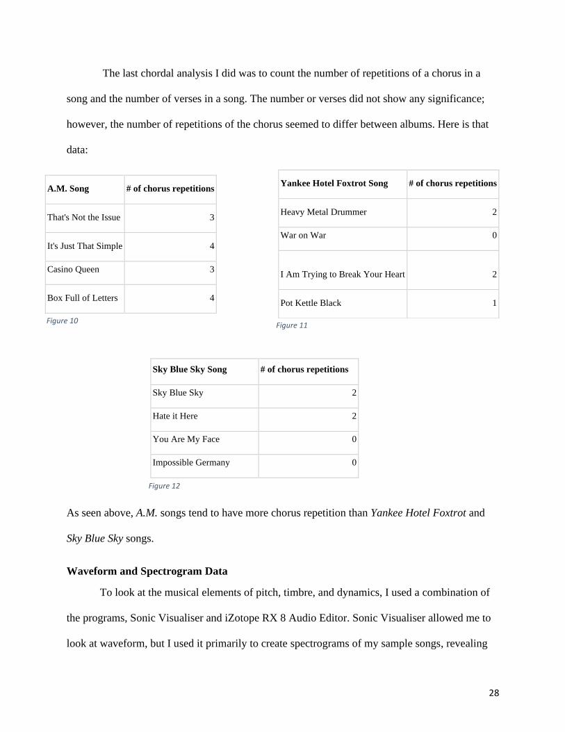
The last chordal analysis I did was to count the number of repetitions of a chorus in a

song and the number of verses in a song. The number or verses did not show any significance;

however, the number of repetitions of the chorus seemed to differ between albums. Here is that

data:

As seen above, A.M. songs tend to have more chorus repetition than Yankee Hotel Foxtrot and

Sky Blue Sky songs.

Waveform and Spectrogram Data

To look at the musical elements of pitch, timbre, and dynamics, I used a combination of

the programs, Sonic Visualiser and iZotope RX 8 Audio Editor. Sonic Visualiser allowed me to

look at waveform, but I used it primarily to create spectrograms of my sample songs, revealing

Yankee Hotel Foxtrot Song # of chorus repetitions


War on War 0

I Am Trying to Break Your Heart 2

Pot Kettle Black 1

A.M. Song # of chorus repetitions

That's Not the Issue 3


Casino Queen 3


Figure 10 Figure 11

Sky Blue Sky Song # of chorus repetitions

Sky Blue Sky 2

Hate it Here 2

You Are My Face 0


Figure 12

29

the overtone structure and intensity of the frequencies. These programs provide a visual means of

analyzing frequencies of music over time and the intensity of those frequencies. It is important to

keep in mind that these images do show us what we hear, but provide an acoustic basis for our

musical perceptions. Though I noticed many differences visually, it was difficult for me to pull

usable numerical data from these pictures, especially since I needed data that encapsulated the

entire song. Perhaps with additional software or technology elements like peak frequency or

average frequency could be quickly determined from a spectrogram. Here is an example of one

of my spectrograms, “Hate it Here” from Sky Blue Sky

Figure 13

This sample snapshot only shows about 20 seconds of the song. The left black bar

denotes frequencies in Hz and the colors show intensity, blue being the least intensity and red

being highest.

iZotope RX 8 Audio Editor can perform the same functions as Sonic Visualiser, but since

it was designed to actually edit and manipulate audio, it has several additional useful features.

The features I found to be the most helpful was the waveform stat feature. After importing an

30

audio file into the software, the program gave me statistical feedback of several features related

to the way the audio was mixed. Here is a screenshot of the waveform stats from Yankee Hotel

Foxtrot’s “War on War”

Figure 14

Comparing these statistics within and between albums, patterns emerge for the true peak

level and loudness range. The true peak level, measured in decibels, is the maximum point that a

waveforms signal reaches. It is a way to measure loudness in digital audio, and typically the

threshold for this measurement is 0 and anything above 0 is at risk of audio distortion or sample

clipping. Furthermore, music streaming service platforms may have a preferred maximum true

peak level limit. For this reason, many producers mix their audio to negative true peak levels.

Generally, high true peak levels show that music is more dynamic. When looking at these

waveform statistics for each album, both A.M. and Sky Blue Sky were mixed to negative true

peak levels while Yankee Hotel Foxtrot songs seem to be all mixed to positive true peak levels.

Here are my sample songs with their respective true peak levels:

31

For my samples, I averaged the left and right true peak levels. There does not appear to

be much difference between the true peak levels in Sky Blue Sky and A.M. songs upon first

glance, but when tested for significance, these two albums could be differentiated from Yankee

Yankee Hotel Foxtrot Song True Peak Level (left and right averaged) (dB)

Heavy Metal Drummer 0.215

War on War 0.14

I Am Trying to Break Your Heart 0.045

Pot Kettle Black 0.185

Figure 15

Sky Blue Sky Songs True Peak Level (average of left and right) (dB)

Sky Blue Sky -1.07

Hate it Here -0.06

You Are My Face -0.8

Impossible Germany -0.895

Figure 16

A.M. Song True Peak Level (left and right averaged) (dB)

That's Not the Issue -0.95

It's Just That Simple -0.97

Casino Queen -0.555

Box Full of Letters -0.92

Figure 17

32

Hotel Foxtrot in this way. The other variable I focused on was the loudness range measured in

loudness units (LU for short). Instead of measuring a peak loudness, this variable measures the

range, or extent to which loudness changes over the course of the song. Loudness units differ

from decibels in the sense that decibels measure air pressure generatd by the physical signal,

wheras LUs are psychophysical measurements based upon perceptual research. Each LU is

equivalent to 1 decibel of air pressure. Generally, tracks that have a loudness range between 6

and 10 LU have considerable loudness difference between sections, and tracks that have a

loudness range below 4 tend to be more static in loudness.

A.M. Song Loudness Range (LU)

That's Not the Issue 2.3

It's Just That Simple 4.1

Casino Queen 2.5

Box Full of Letters 1.7

Figure 19

Yankee Hotel Foxtrot Song Loudness Range (LU)


War on War 4.6



Figure 18

Sky Blue Sky Song Loudness Range (LU)

Sky Blue Sky 4.8

Hate it Here 5.6

You Are My Face 10.1

Impossible Germany 6.1

Figure 20

33

Comparing these tables, there seems to be dynamical differences between these 3 albums,

especially between A.M. and Sky Blue Sky.

Lyrical and Structural Data

In my data collection, I wanted to also consider lyrical and structural variables that could

show evolution between Wilco’s albums. In addition to looking at verse and chorus repetitions, I

studied the number of lines in the chorus, the number of lines in the verses, and total number of

lines repeated per song. To do this, I cross-referenced lyrics from “Genius Lyrics” and “AZ

Lyrics” which both break songs into their intro/verse/chorus type of form. All three of these data

sets seemed to have very little correlation with each other. For example, here is the data I

collected for the number of lines in the chorus:

A.M. Song # of lines in chorus



Casino Queen 4


Figure 22

Yankee Hotel Foxtrot Song # of lines in chorus


War on War 4

I Am Trying to Break Your

Heart

0

Pot Kettle Black 5

Figure 21

Sky Blue Sky Song # of lines in chorus

Sky Blue Sky 7

Hate it Here 3

You Are My Face 0


Figure 23

34

There is no apparent consistency within albums for this data set, so there cannot even begin to be

a comparison from album to album.

Other

Other than drawing data from these categories mentioned above, I collected data on each

sample song’s tempo and length. The website, “GetSongbpm” has tempo data for several bands

and artists, and I used their data to compare song tempo using beats per minute. To check for

accuracy, I verified the website’s results using a metronome for my 16 songs, and finding it to be

accurate, I used the website alone when testing my models. Below is the tempo data I collected:

A.M. Song Tempo (BPM)



Casino Queen 126


Sky Blue Sky Song Tempo (BPM)

Sky Blue Sky 116

Hate it Here 80

You Are My Face 80


Figure 24 Figure 25

Yankee Hotel Foxtrot Song Tempo (BPM)


War on War 131


Heart

85

Pot Kettle Black 123

Figure 26

35

This data shows consistency within albums, although there may be an outlier like “I Am

Trying to Break Your Heart” in Yankee Hotel Foxtrot. A single outlier does not necessarily

indicate unusable data, though. “GetSongbpm” also has song length data, and converting the

minute:seconds time to minutes in a decimal form made the song lengths easily comparable. This

is the data I collected for song length:

A.M. Song Song length (minutes)

That's Not the Issue 3.35

It's Just That Simple 3.77

Casino Queen 2.75

Box Full of Letters 3.1

Figure 28

Figure 29

Yankee Hotel Foxtrot Song Song length (minutes)


War on War 3.8


Pot Kettle Black 4

Figure 27

Sky Blue Sky Song Song length (minutes)

Sky Blue Sky 3.38

Hate it Here 4.52

You Are My Face 4.62

Impossible Germany 5.45

36

Data Summary

After examining several layers of data in my samples, I eliminated several based off of

low within-album consistency. When doing this, I kept the normal distribution curve in mind

(explained in next section) which is a way of describing the way data should fall around the

mean in order to be considered “normally distributed.” Linear Discriminant Analysis requires

input data that is normally distributed, so I tried to keep this in mind moving forward in my

analysis. In the end, the variables I decided to continue to my two-tailed t-testing are: instrument

number, number of chorus repetitions, number of minor chords per song, true peak level,

loudness range, tempo, and song length.

All these charts are scattered above… should i put them all in the summary part also/ move them

here instead?

Variable Elimination – Student’s Two Tailed t-Test

Student’s t-test is a variation of t-distribution that is used specifically to measure how

significant the difference between groups is. It signifies if difference between the means is

meaningful or if it possibly occurred by chance. In this part of my process, I use it to check

which variables show significant difference between albums. Student’s t-test is unique in that it

can specifically be used for small sample sizes. When working with albums, you only have a

small sample size to work with, so the student’s t-test fits our data best. In this project, student’s

t-tests were used to decide which variables qualified as significant in distinguishing between

albums. Furthermore, I decided to use a two-tailed test over a one-tailed test because the two-

tailed test checks for possible values on both sides of the curve and therefore can give a more

accurate significance level. Several variables were tested, and those that worked were applied in

my models. Here are the steps to carrying out a student’s t-test:

37

1: calculate the pooled standard deviation: 𝑆𝑝

• This is the weighted average of standard deviations for the two samples

• This formula is as follows: 𝑆𝑝 = √(𝑛𝑥−1)𝑠𝑥

2+(𝑛𝑦−1)𝑠𝑦2

𝑛𝑥+𝑛𝑦−2

o 𝑛𝑥 = size of sample x

o 𝑛𝑦 = size of sample y

o 𝑠𝑥2=variance of sample x

o 𝑠𝑦2=variance of sample y

2: calculate the test statistic

• This is the ratio between the difference between the groups and difference within the

groups. Essentially, a larger t-scores indicates the groups are different while a small t-

score indicates the groups are similar

• This formula is as follows: 𝑡 =𝑋− 𝑌

𝑆𝑝√1

𝑁𝑥 +

1

𝑁𝑥𝑦

o 𝑋=the mean of sample x

o 𝑌= the mean of sample y

o 𝑆𝑝 = pooled standard deviation

o 𝑁𝑥 = size of sample x

o 𝑁𝑦 = size of sample y

3: calculate the P-value

• This is the area under the Student’s t curve with ( 𝑛𝑥 + 𝑛𝑦 − 2 ) degrees of freedom. We

want to know how big or small our test statistic is and this p value will tell us the

probability that the difference occurred by chance

• Using the degrees of freedom, consult a Student’s t table to find the area under the curve

under both tails (this is what makes this two tailed). This value would be the p value.

• Typically these p values can be looked at in comparison to 0.1, 0.05, and 0.01

o If p>0.1 the result is said to not be significant

o If 0.1<p<0.05 p is said to be slightly significant

o If 0.5<p<0.01 p is said to be significant

o If p<0.01 p is said to be very significant

• If this p value is, say, 0.02, this means the difference between the groups has a 0.02

probability of being by chance. This means significance!

38

Here is an example of how I used student’s t-test for my model:

Yankee Hotel Foxtrot Song (x) Instrument # Sky Blue Sky Song (y) Instrument #

Heavy Metal Drummer 11 Sky Blue Sky 8

War on War 12 Hate it Here 7

I Am Trying to Break Your Heart 13 You Are My Face 7

Pot Kettle Black 10 Impossible Germany 6

Figure 30

𝑛𝑥 4

𝑛𝑦 4

𝑠𝑥2 1.67

𝑠𝑦2 0.67

𝑋 11.5

𝑌 7

𝑆𝑝 (about) 1.0817

t 5.89

p 0.0053

Testing data between number of instruments in Yankee Hotel Foxtrot and Sky Blue Sky, there

seems to be a very statistically significant difference in the data sets. This signifies usable data

for my model.

Running these t-tests revealed there were no variables that showed significance between all 3

albums, so this is the point where I decided to compare the albums in pairs rather than all three

together.

The results of my usable-data student t-tests are summarized in Figure 31, 32 and 33:


vs. Sky Blue Sky

T (rounded to the

nearest hundredth)

p Significance

Instrument # 5.89 0.0053 Very significant

# of minor chords/song -3.46 0.0067 Very significant

True peak level 3.78 0.009198 Very significant

Figure 31

39

A.M. vs. Sky Blue Sky T (rounded to the

nearest hundredth)

p Significance

BPM 3.12 0.020573 significant

Song Length 2.67 0.0394 Significant

Loudness range -3.12 0.020909 Significant

Figure 32

A.M. vs. Yankee Hotel

Foxtrot

T (rounded to the

nearest hundredth)

p Significance

Instrument # -7.2 0.000363 Very significant

True peak level -9.46 0.00008 Very significant

# of chorus repetitions 4.02 0.00692 Very significant

Figure 33

Variable Classification – LDA

Fi=Mi·C-1·XT−0.5·Mi·C-1·MiT+ln(Pi)

Fi=discriminant function of class i

Mi=mean vector of class i

XT=new comer’s data

C-1=inner-class variance

Pi=prior probability of class i

The variable classification in this thesis will occur through three separate algorithms. The

first algorithm will compare Yankee Hotel Foxtrot and Sky Blue Sky, the second will compare

A.M. and Sky Blue Sky and the third will compare A.M. and Yankee Hotel Foxtrot. The first

algorithm will be presented with great detail and explanation followed by the other two in less

detail.

40

For Algorithm 1, class 1 will be Yankee Hotel Foxtrot and class 2 will be Sky Blue Sky.

To build the discriminant function by hand, I will be using matrices as a simple and organized

way to work with this level of data. We will find a discriminant function (F1 and F2) for each

class using the training data below and graph these functions to find our classification line. After

the classification line has been identified, a song of an unknow class can be plugged into the

discriminant function and its coordinate point in comparison to the classification line will

indicate which class the song predictably belongs to.

Training Data

Yankee Hotel Foxtrot Song Instrument # Sky Blue Sky Song Instrument #



I Am Trying to Break Your Heart 13 You Are My Face 7

Pot Kettle Black 10 Impossible Germany 6

Figure 34

Yankee Hotel Foxtrot Song

# of minor

chords/song Sky Blue Sky Song

# of minor

chords/song




Heart 1 You Are My Face 4

Pot Kettle Black 2

Impossible

Germany 3

Figure 35

41

Yankee Hotel

Foxtrot Song

True Peak Level (average of

left and right) (dB)

Sky Blue Sky

Song

True Peak Level (average of

left and right) (dB)

Heavy Metal

Drummer 0.215 Sky Blue Sky -1.07

War on War 0.14 Hate it Here -0.06

I Am Trying to Break

Your Heart 0.045

You Are My

Face -0.8


Impossible

Germany -0.895

Figure 36

Global mean calculations

The first calculation we make is to find the “Global Means” matrix. This matrix holds mean data

between the two classes.

Instrument #: (11+12+13+10+8+7+7+6)/(4+4)=9.25

# Of Minor Chords/Song: (0+1+1+2+3+2+4+3)/(4+4)=2

True Peak Level: (0.215+0.14+0.045+0.185+(-1.07)+(-0.06)+(-0.8)+(-0.895))/(4+4)= -0.28

Resulting matrix:

M=[9.25 2 -0.28]

Calculating M1

Next, we calculate M1, the mean vector of class 1. This is simply the mean of each variable we

are looking at but only in Yankee Hotel Foxtrot.

Instrument #: (11+12+13+10)/4=11.5

# Of Minor Chords/Song: (0+1+1+2)/4=1

42

True Peak Level: (0.215+0.14+0.045+0.185)/4=0.146

The resulting matrix:

M1=[11.5 1 0.14625]

Calculating C1

Next, we find, the covariance matrix for class 1 (Yankee Hotel Foxtrot).

To do this, we want to find the variance in our data: the way our actual data deviates from the

global mean. We want this scatter matrix to minimize variability within the class. We will

subtract the respective global mean from the actual data.

# of instruments # of minor chords True Peak Level

11-9.25=1.75 0-2= -2 0.215-(-0.28)=0.495

12-9.25=2.75 1-2= -1 0.14-(-0.28)=0.42

13-9.25=3.75 1-2= -1 0.045-(-0.28)=0.325

10-9.25=0.75 2-2=0 0.185-(-0.28)=0.465

Figure 37

To build our actual C1, matrix, we will multiply the product of a matrix formed from the data

above and that same matrix transposed to ¼ (4 is number of variables we are using). Multiplying

by the transpose here will provide us with a square (n x n) matrix which result in a symmetric

and easier-to-use matrix. This will allow us, later, to determine the inverse of C.

C1= ¼ x [1.75 2.75 3.75 0.75−2 −1 −1 0

0.495 0.42 0.325 0.465] x [

1.75 −2 0.4952.75 −1 0.423.75 −1 0.3250.75 0 0.465

]

43

When we do this,

C1=|6.3125 −2.5 0.89719

−2.5 1.5 −0.433750.89719 −0.43375 0.18582

| (supposed to be brackets)

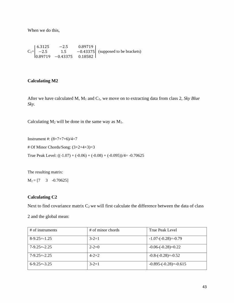
Calculating M2

After we have calculated M, M1 and C1, we move on to extracting data from class 2, Sky Blue

Sky.

Calculating M2 will be done in the same way as M1.

Instrument #: (8+7+7+6)/4=7

# Of Minor Chords/Song: (3+2+4+3)=3

True Peak Level: ((-1.07) + (-0.06) + (-0.08) + (-0.095))/4= -0.70625


M2 = [7 3 -0.70625]

Calculating C2

Next to find covariance matrix C2 we will first calculate the difference between the data of class

2 and the global mean:

# of instruments # of minor chords True Peak Level

8-9.25=-1.25 3-2=1 -1.07-(-0.28)=-0.79

7-9.25=-2.25 2-2=0 -0.06-(-0.28)=0.22

7-9.25=-2.25 4-2=2 -0.8-(-0.28)=-0.52

6-9.25=-3.25 3-2=1 -0.895-(-0.28)=-0.615

44

Now to calculate C2

C2 = 1/4 x [−1.25 −2.25 −2.25 −3.25

1 0 2 1−0.79 0.22 −0.52 −0.615

] x [

−1.25 1 −0.79−2.25 0 0.22−2.25 2 −0.52−3.25 1 −0.615

]

C2 = [5.5625 −2.25 0.91531−2.25 1.5 −0.61125

0.91531 −0.61125 0.33028]

Calculating C and C-1

In summary, we have now calculated M, M1, M2, C1, and C2. We will now use these for the

calculation of C, C-1 and our F1 and F2.

M = [9.25 2 -0.28]

M1 = [11.5 1 0.14625]

M2 = [7 3 -0.70625]

C1 = |6.3125 −2.5 0.89719

−2.5 1.5 −0.433750.89719 −0.43375 0.18582

|

C2 = [5.5625 −2.25 0.91531−2.25 1.5 −0.61125

0.91531 −0.61125 0.33028]

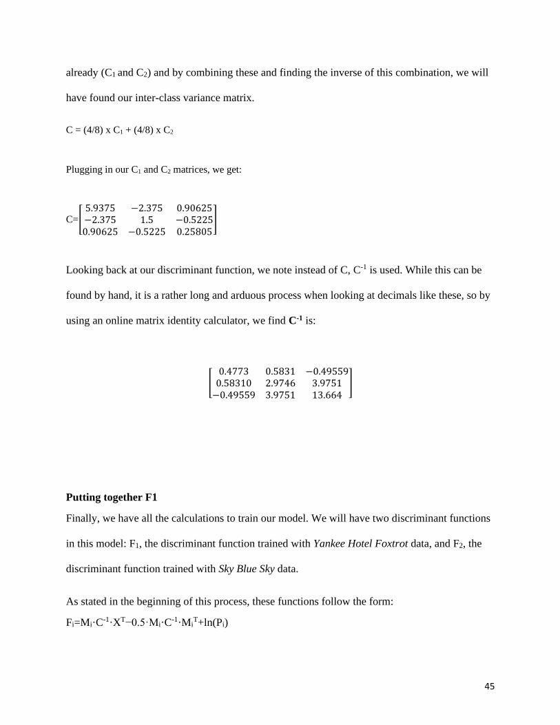
C-1 is our inter-class variance which we can think of as the variance between our two classes. The

purpose of this calculation is to maximize this variance. We calculated intra-class variance

45

already (C1 and C2) and by combining these and finding the inverse of this combination, we will

have found our inter-class variance matrix.

C = (4/8) x C1 + (4/8) x C2

Plugging in our C1 and C2 matrices, we get:

C=[5.9375 −2.375 0.90625−2.375 1.5 −0.52250.90625 −0.5225 0.25805

]

Looking back at our discriminant function, we note instead of C, C-1 is used. While this can be

found by hand, it is a rather long and arduous process when looking at decimals like these, so by

using an online matrix identity calculator, we find C-1 is:

[0.4773 0.5831 −0.49559

0.58310 2.9746 3.9751−0.49559 3.9751 13.664

]

Putting together F1

Finally, we have all the calculations to train our model. We will have two discriminant functions

in this model: F1, the discriminant function trained with Yankee Hotel Foxtrot data, and F2, the

discriminant function trained with Sky Blue Sky data.

As stated in the beginning of this process, these functions follow the form:

Fi=Mi·C-1·XT−0.5·Mi·C

-1·MiT+ln(Pi)

46

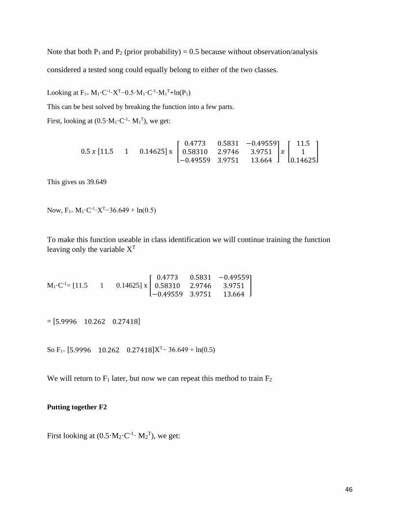
Note that both P1 and P2 (prior probability) = 0.5 because without observation/analysis

considered a tested song could equally belong to either of the two classes.

Looking at F1= M1·C-1·XT−0.5·M1·C-1·M1T+ln(P1)

This can be best solved by breaking the function into a few parts.

First, looking at (0.5·M1·C-1· M1T), we get:

0.5 𝑥 [11.5 1 0.14625] x [0.4773 0.5831 −0.49559

0.58310 2.9746 3.9751−0.49559 3.9751 13.664

] 𝑥 [11.5

10.14625

]

This gives us 39.649

Now, F1= M1·C-1·XT−36.649 + ln(0.5)

To make this function useable in class identification we will continue training the function

leaving only the variable XT

M1·C-1= [11.5 1 0.14625] x [0.4773 0.5831 −0.49559

0.58310 2.9746 3.9751−0.49559 3.9751 13.664

]

= [5.9996 10.262 0.27418]

So F1= [5.9996 10.262 0.27418]XT− 36.649 + ln(0.5)

We will return to F1 later, but now we can repeat this method to train F2

Putting together F2

First looking at (0.5·M2·C-1· M2

T), we get:

47

0.5 𝑥 [7 3 − 0.70625] 𝑥 [0.47717 0.58294 −0.495450.58297 2.9744 3.9753

−0.49539 3.9754 13.664] 𝑥 [

73

−0.70625]

This gives us 34.752

Now, F2= M2·C-1·XT- 34.76 + ln(0.5)

To make this function useable in class identification we will continue training the function

leaving only the XT

M2·C-1= [7 3 -0.70625] x [0.47717 0.58294 −0.495450.58297 2.9744 3.9753

−0.49539 3.9754 13.664]

= [5.4390 10.196 −1.1925]

Now, F2= [5.4390 10.196 −1.1925]·XT- 34.752 + ln(0.5)

Summary and Test

In summary our two discriminant functions are:

F1= [5.9996 10.262 0.27418]XT− 36.649 + ln(0.5)

F2= [5.4390 10.196 −1.1925]·XT- 34.752 + ln(0.5)

The next step is to plug my training data back into the two discriminant functions. For example,

if we want to find the F1 and F2 values of “Heavy Metal Drummer,” we would set up our data in a

matrix as X= [11 0 0.215] (11 instruments, 0 minor chords, and a true peak level of

0.215). So,

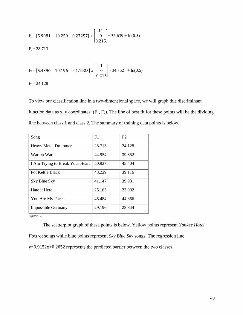
48

F1= [5.9981 10.259 0.27257] x [110

0.215]− 36.639 + ln(0.5)

F1= 28.713

F2= [5.4390 10.196 −1.1925] x [10

0.215] - 34.752 + ln(0.5)

F2= 24.128

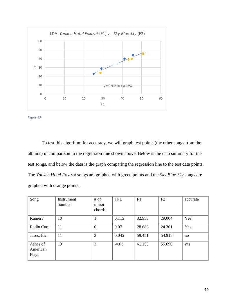
To view our classification line in a two-dimensional space, we will graph this discriminant

function data as x, y coordinates: (F1, F2). The line of best fit for these points will be the dividing

line between class 1 and class 2. The summary of training data points is below.

Song F1 F2

Heavy Metal Drummer 28.713 24.128

War on War 44.954 39.852

I Am Trying to Break Your Heart 50.927 45.404

Pot Kettle Black 43.229 39.116

Sky Blue Sky 41.147 39.931

Hate it Here 25.163 23.092

You Are My Face 45.484 44.366

Impossible Germany 29.196 28.844

Figure 38

The scatterplot graph of these points is below. Yellow points represent Yankee Hotel

Foxtrot songs while blue points represent Sky Blue Sky songs. The regression line

y=0.9152x+0.2652 represents the predicted barrier between the two classes.

49

Figure 39

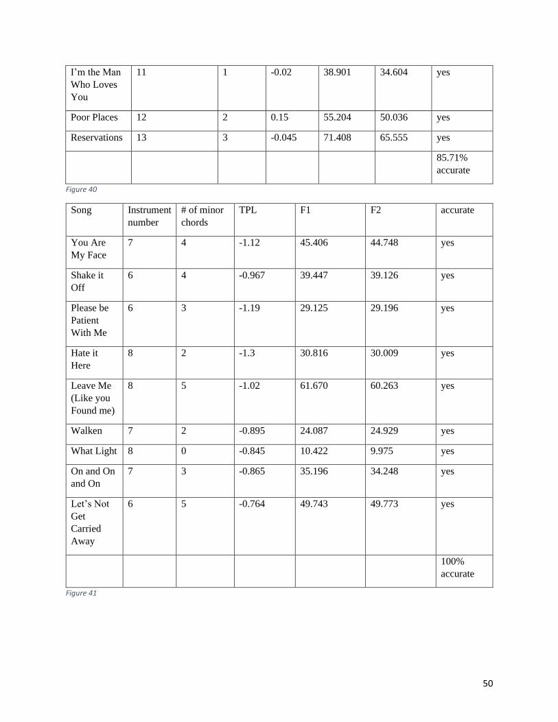
To test this algorithm for accuracy, we will graph test points (the other songs from the

albums) in comparison to the regression line shown above. Below is the data summary for the

test songs, and below the data is the graph comparing the regression line to the test data points.

The Yankee Hotel Foxtrot songs are graphed with green points and the Sky Blue Sky songs are

graphed with orange points.

Song Instrument

number

# of

minor

chords

TPL F1 F2 accurate

Kamera 10 1 0.115 32.958 29.004 Yes

Radio Cure 11 0 0.07 28.683 24.301 Yes

Jesus, Etc. 11 3 0.045 59.451 54.918 no

Ashes of

American

Flags

13 2 -0.03 61.153 55.690 yes

y = 0.9152x + 0.2652

0

10

20

30

40

50

60

0 10 20 30 40 50 60

F2

F1

LDA: Yankee Hotel Foxtrot (F1) vs. Sky Blue Sky (F2)

50

I’m the Man

Who Loves

You

11 1 -0.02 38.901 34.604 yes

Poor Places 12 2 0.15 55.204 50.036 yes

Reservations 13 3 -0.045 71.408 65.555 yes

85.71%

accurate

Figure 40

Song Instrument

number

# of minor

chords

TPL F1 F2 accurate

You Are

My Face

7 4 -1.12 45.406 44.748 yes

Shake it

Off

6 4 -0.967 39.447 39.126 yes

Please be

Patient

With Me

6 3 -1.19 29.125

29.196 yes

Hate it

Here

8 2 -1.3 30.816 30.009 yes

Leave Me

(Like you

Found me)

8 5 -1.02 61.670 60.263 yes

Walken 7 2 -0.895 24.087 24.929 yes

What Light 8 0 -0.845 10.422 9.975 yes

On and On

and On

7 3 -0.865 35.196 34.248 yes

Let’s Not

Get

Carried

Away

6 5 -0.764 49.743 49.773 yes

100%

accurate

Figure 41

51

Figure 42

Observing the graph, all songs appear to be categorized correctly, except for the song, “Jesus,

Etc.” (59.451, 54.918). This point is on the line, but is more above the line than below. To verify

points that are on or close to the line, we can plug are actual F1 value into the regression

equation and compare the resulting y value to our actual F2 value. If we wanted to verify “Jesus,

Etc.” is in fact classified in class 2, we can fill our regression equation as follows:

y=0.9152(59.451) + 0.265→y=54.675. Since 54.675<54.918 (actual F2 value) our “Jesus, Etc.”

point is above the line. Overall accuracy for this algorithm is 93.7%.

52

Algorithm 2: A.M. (F1) vs Sky Blue Sky (F2)

A.M. Song BPM Sky Blue Sky Song BPM

That's Not the Issue 119 Sky Blue Sky 116

It's Just That Simple 124 Hate it Here 80

Casino Queen 126 You Are My Face 80

Box Full of Letters 125 Impossible Germany 104

Figure 43

A.M. Song Loudness Range (LU) Sky Blue Sky Song Loudness Range (LU)

That's Not the Issue 2.3 Sky Blue Sky 4.8

It's Just That Simple 4.1 Hate it Here 5.6

Casino Queen 2.5 You Are My Face 10.1

Box Full of Letters 1.7 Impossible Germany 6.1

Figure 44

A.M. Song Song length (minutes) Sky Blue Sky Song Song length (minutes)

That's Not the Issue 3.35 Sky Blue Sky 3.38

It's Just That Simple 3.77 Hate it Here 4.52

Casino Queen 2.75 You Are My Face 4.62

Box Full of Letters 3.1 Impossible Germany 5.45

Figure 45

Global Mean Calculations

Resulting matrix:

M=[109.25 4.65 3.8675]

Calculating M1

53

Resulting matrix:

M1=[123.5 2.65 3.2425]

Calculating C1

BPM Loudness ranges Song length

119-109.25=9.75 2.3-4.65=-2.35 3.35-3.8675=-0.5175

124-109.25=14.75 4.1-4.65-0.55 3.77-3.8675=-0.0975

126-109.25=16.75 2.5-4.65=-2.15 2.75-3.8675=-1.1175

125-109.25=15.75 1.7-4.65=-2.95 3.1-3.8675=-0.7675

C1= [210.3125 −28.375 −9.3225−28.375 4.7875 1.484125

−9.321525 1.48389 0.528742]

Calculating M2

M2=[95 6.65 4.4925]

BPM Loudness ranges Song length

116-109.25=6.75 4.8-4.65=0.15 3.38-3.8675=-0.4875

80-109.25=-29.25 5.6-4.65=0.95 4.52-3.8675=0.6525

80-109.25=-29.25 10.1-4.65=5.45 4.62-3.8675=0.7525

104-109.25=-5.25 6.1-4.65=1.45 5.45-3.8675=1.5825

C2=[446.0625 −48.45 −13.17375

−48.45 8.1825 1.735625−13.17375 1.735625 0.93349375

]


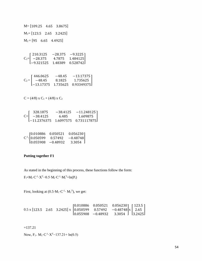
54

M= [109.25 4.65 3.8675]

M1= [123.5 2.65 3.2425]

M2 = [95 6.65 4.4925]

C1=[210.3125 −28.375 −9.3225−28.375 4.7875 1.484125

−9.321525 1.48389 0.528742]

C2 = [446.0625 −48.45 −13.17375

−48.45 8.1825 1.735625−13.17375 1.735625 0.93349375

]

C = (4/8) x C1 + (4/8) x C2

C=[328.1875 −38.4125 −11.248125−38.4125 6.485 1.609875

−11.2376375 1.6097575 0.731117875]

C-1:[0.010886 0.050521 0.0562300.050599 0.57492 −0.487480.055908 −0.48932 3.3054

]

Putting together F1




0.5 x [123.5 2.65 3.2425] x [0.010886 0.050521 0.0562300.050599 0.57492 −0.487480.055908 −0.48932 3.3054

]x [123.52.65

3.2425]

=137.21

Now, F1= M1·C-1·XT−137.21+ ln(0.5)

55

𝑀1𝐶−1 = [123.5 2.65 3.2425] x [0.010886 0.050521 0.0562300.050599 0.57492 −0.487480.055908 −0.48932 3.3054

]

=[1.6598 6.1763 16.370]

So, F1=[1.6598 6.1763 16.370]XT -137.21+ln0.5

Putting together F2

First looking at (0.5·M2·C-1· M2T), we get:

0.5 x [95 6.65 4.4925] x [0.010886 0.050521 0.0562300.050599 0.57492 −0.487480.055908 −0.48932 3.3054

] x [95

6.654.4925

]

=136.47

Now, F2= M2·C-1·XT- 136.47 + ln(0.5)

𝑀2𝐶−1 = [95 6.65 4.4925]x[0.010886 0.050521 0.0562300.050599 0.57492 −0.487480.055908 −0.48932 3.3054

]

=[1.6218 6.4244 16.95]

Now, F2=[1.6218 6.4244 16.95]XT -136.47+ln0.5

Summary and Test


F1=[1.6598 6.1763 16.370]XT -137.21+ln0.5

F2=[1.6218 6.4244 16.95]XT -136.47+ln0.5

56

The training data plugged back into these functions gives us these values:

Song F1 F2

That’s Not the Issue 128.657 127.387

It’s Just That Simple 154.947 154.177

Casino Queen 131.657 129.857

Box Full of Letters 130.817 129.027

Sky Blue Sky 139.607 139.097

Hate it Here 103.097 105.167

You Are My Face 132.887 135.777

Impossible Germany 161.607 163.067

Figure 46

Graphically this gives us a regression line of y=0.9867 + 1.8407. A.M. songs are represented by

green dots, and Sky Blue Sky songs are represented by blue dots.

Figure 47

y = 0.9867x + 1.8407

0

20

40

60

80

100

120

140

160

180

0 20 40 60 80 100 120 140 160 180

F2

F1

LDA: A.M. vs. Sky Blue Sky

57

Song BPM Loudness

range

Song Length

(seconds)

F1 F2 accurate

You Are My Face 80 10.1 4.633 133.107 135.997 yes

Shake it Off 126 12.2 5.67 239.397 241.667 yes

Please be Patient With

Me

91 9.4 3.6167 130.397 132.117 yes

Hate it Here 80 5.6 4.51667 103.407 105.117 yes

Leave Me (Like you

Found me)

102 4.5 4.15 127.127 127.517 yes

Walken 167 6.3 4.433 249.287 250.767 yes

What Light 175 9.8 3.583 271.747 270.347 yes

On and On and On 115 11 4 186.397 190.119 yes

100% accuracy

Figure 48

Song BPM Loudness

range

Song Length

(seconds)

F1 F2 accurate

I Must Be High 120 3.6 2.983 124.157 123.837 yes

Shouldn’t Be

Ashamed

111 6.3 3.483 142.097 142.367 no

Pick Up The Change 110 2.2 2.933 106.277 105.087 yes

I Thought I Held You 97 4.2 3.817 111.827 111.387 Yes

That’s Not the Issue 119 2.3 3.35 128.097 127.387 Yes

Should’ve Been in

Love

117 2.5 3.6 130.667 129.667 yes

Passenger Side 183 1.7 3.567 234.727 231.007 yes

Dash 7 120 12 3.483 192.397 193.587 no

Blue Eyed Soul 135 7.2 4.083 197.477 197.247 no

66.67%

accuracy

Figure 49

58

Here, A.M. songs are depicted with yellow points and Sky Blue Sky songs are depicted with blue

points. Upon zooming into the line, all points are classified correctly except the songs “Shouldn’t

Be Ashamed” (130.667, 129.667), “Dash 7” (192.397, 193.587) and “Blue Eyed Soul” (197.477,

197.247). The overall accuracy of algorithm 2 is 82.35%.

Algorithm 3: A.M. (F1) vs. Yankee Hotel Foxtrot (F2)

A.M. Song Instrument # Yankee Hotel Foxtrot Song Instrument #

That's Not the Issue 7 Heavy Metal Drummer 11

It's Just That Simple 6 War on War 12

Casino Queen 6 I Am Trying to Break Your Heart 13

Box Full of Letters 5 Pot Kettle Black 10

Figure 50

59

Figure 51

A.M. Song # of chorus repetitions Yankee Hotel Foxtrot Song # of chorus repetitions

That's Not the Issue 3 Heavy Metal Drummer 2

It's Just That Simple 4 War on War 0

Casino Queen 3 I Am Trying to Break Your Heart 2

Box Full of Letters 4 Pot Kettle Black 1

Figure 52

Global mean calculations

Resulting matrix:

M=[8.75 2.375 -0.35125]

Calculating M1

Resulting matrix:

M1=[6 3.5 -0.84875]

A.M. Song

True Peak Level (left and right

averaged) (dB)


Song

True Peak Level (left and

right averaged)

That's Not the

Issue -0.95 Heavy Metal Drummer 0.215

It's Just That

Simple -0.97 War on War 0.14

Casino Queen -0.555

I Am Trying to Break

Your Heart 0.045

Box Full of

Letters -0.92 Pot Kettle Black 0.185

Figure 53

60

Calculating C1

# of instruments # of chorus repetitions True Peak Level

7-8.75=-1.75 3-2.375=0.625 -0.95-(-0.35125)=-0.59875

6-8.75=-2.75 4-2.375=1.625 -0.97-(-0.35125)=-0.61875

6-8.75=-2.75 3-2.375=0.625 -0.555-(-0.35125)=-0.20375

5-8.75=-3.75 4-2.375=1.625 -0.92-(-0.35125)=-0.56875

C1= ¼ x [−1.75 −2.75 −2.75 −3.750.625 1.625 0.625 1.625

−0.59875 −0.61875 −0.20375 −0.56875] x [

−1.75 0.625 −0.59875−2.75 1.625 −0.61875−2.75 0.625 −0.20375−3.75 1.625 −0.56875

]

C1=[8.0625 −3.3438 1.3606

−3.3438 1.5156 −0.607811.3606 −0.60781 0.27659

]

Calculating M2


M2 = [11.5 1.25 0.14625]

Calculating C2

# of instruments # of chorus repetitions True Peak Level

11-8.75=2.25 2-2.375=-0.375 0.215-(-0.35125)=0.56625

12-8.75=3.25 0-2.375=-2.375 0.14-(-0.35125)=0.49125

13-8.75=4.25 2-2.375=-0.375 0.045-(-0.35125)=0.39625

10-8.75=1.25 1-2.375=-1.375 0.185-(-0.35125)=0.53625

C2 = 1/4 x [2.25 3.25 4.25 1.25

−0.375 −2.375 −0.375 −1.3750.56625 0.49125 0.39625 0.53625

] x [

2.25 −0.375 0.566253.25 −2.375 0.491254.25 −0.375 0.396251.25 −1.375 0.53625

]

C2 = [8.8125 −2.9688 1.3063

−2.9688 1.9531 −0.566251.3063 −0.56625 0.25164

]

61


M=[8.75 2.375 -0.35125]

M1= [6 3.5 -0.84875]

M2 = [11.5 1.25 0.14625]

C1=[8.0625 −3.3438 1.3606

−3.3438 1.5156 −0.607811.3606 −0.60781 0.27659

]

C2 = [8.8125 −2.9688 1.3063

−2.9688 1.9531 −0.566251.3063 −0.56625 0.25164

]

C = (4/8) x C1 + (4/8) x C2

C=[8.4375 −3.1563 1.3335

−3.1563 1.7344 −0.587031.3335 −0.58703 0.26412

]

C-1:[0.61768 0.27683 −2.50320.27683 2.4518 4.0519−2.5032 4.0519 25.430

]

Putting together F1




62

0.5 𝑥 [6 3.5 − 0.84875] x [0.61768 0.27683 −2.50320.27683 2.4518 4.0519−2.5032 4.0519 25.430

] 𝑥 [6

3.5−0.84875

]

= 41.819

Now, F1= M1·C-1·XT−41.819+ ln(0.5)

M1·C-1= [6 3.5 − 0.84875]x [0.61768 0.27683 −2.50320.27683 2.4518 4.0519−2.5032 4.0519 25.430

]

= [6.7996 6.8032 −22.421]

So F1= [6.7996 6.8032 −22.421]XT− 41.819 + ln(0.5)

Putting together F2

First looking at (0.5·M2·C-1· M2T), we get:

0.5 𝑥 [11.5 1.25 0.14625] 𝑥 [[0.61768 0.27683 −2.50320.27683 2.4518 4.0519−2.5032 4.0519 25.430

]] 𝑥 [11.51.25

0.14625]

=43.542

Now, F2= M2·C-1·XT- 43.542 + ln(0.5)

M2·C-1=[11.5 1.25 0.14625]x [0.61768 0.27683 −2.50320.27683 2.4518 4.0519−2.5032 4.0519 25.430

]

= [7.0833 6.8409 −20.003]

Now, F2= [7.0833 6.8409 −20.003]·XT- 43.542 + ln(0.5)

Summary and Test


F1= [6.7996 6.8032 −22.421]XT− 41.819 + ln(0.5)

63

F2= [7.0833 6.8409 −20.003]·XT- 43.542 + ln(0.5)

The training data plugged back into the discriminant functions gives us these values:

Song F1 F2

That’s Not the Issue 46.795 44.874

It’s Just That Simple 47.247 45.031

Casino Queen 31.139 29.889

Box Full of Letters 39.326 36.948

Heavy Metal Drummer 41.069 43.062

War on War 35.944 37.964


Heart 58.478 60.625

Pot Kettle Black 28.139 29.738

Figure 54

graphically this gives us a regression line of y=0.9973x + 0.1086. A.M. songs are represented by

green dots, and Yankee Hotel Foxtrot songs are represented by yellow dots.

y = 0.9973x + 0.1086

0

10

20

30

40

50

60

70

0 10 20 30 40 50 60 70

F2

F1

LDA: A.M. (F1) vs. Yankee Hotel Foxtrot (F2)

Figure 55

64

Song Instrument

number

# of chorus

repetitions

TPL F1 F2 accurate

Kamera 10 3 0.115 43.315 44.820 yes

Radio Cure 11 2 0.07 44.321 54.963 yes

Jesus, Etc. 11 3 0.045 51.684 53.304 yes

Ashes of

American

Flags

13 0 -0.03 46.555 48.448 yes

I’m the Man

Who Loves

You

11 3 -0.02 53.142 54.604 yes

Poor Places 12 1 0.15 42.523 44.605 yes

Reservations 13 3 -0.045 67.298 69.275 yes

100%

accurate

Figure 56

Figure 57

Song Instrument

number

# of chorus

repetitions

TPL F1 F2 accurate

I Must Be High 6 0 -0.62 12.187 10.667 yes

Shouldn’t Be

Ashamed

6 3 -0.96 40.219 37.990 yes

Pick Up The

Change

6 3 -0.865 38.089 36.090 yes

I Thought I Held

You

7 2 -0.905 38.983 37.133 yes

Should’ve Been

in Love

5 5 -0.915 46.017 43.689 yes

Passenger Side 7 3 -1.485 58.788 55.575 yes

Dash 7 3 4 -1.5 38.731 34.383 yes

Blue Eyed Soul 7 3 -0.845 44.441 42.773 yes

100%

accurate

65

Figure 58

In this graph, A.M. test songs are marked as orange points while Yankee Hotel Foxtrot test songs

are marked as green. This algorithm appears to classify all the test data with 100% accuracy.

66

Chapter 4: Discussion and Conclusion

Model 1

Model (algorithm) 1 comparing Yankee Hotel Foxtrot to Sky Blue Sky, was based on the

number of instruments used, the frequency of minor chords per song and the average true peak

levels in each song. Each of these variables proved to be very statistically significant in the t-test

portion of the analysis, which resulted in decently high inter-class variance. This is visually

represented in the ways the data points of the training variables do not touch the regression line.

An inter-class variance signifies a larger difference between classes, so the model is likely to

make less errors in classifying an unknown song. The only song to be classified incorrectly using

this model was “Jesus, Etc,” which is likely due to the higher number of minor chords (3), as

compared to the global mean (2), and the relatively low true peak level of the song (0.045),

compared to the mean of class 1. Despite this one misclassification, Model 1appears to be

effective even if one of the three data numbers is very atypical of the correct class, or two

numbers are slightly atypical. The overall tested accuracy of 93.75% proves that these two

albums can, in fact, be distinguished by the number of instruments used, frequency of minor

chords per song, and the average true peak level in each song.

Model 2

Model (algorithm) 2 comparing A.M. and Sky Blue Sky was based on tempo, loudness

range, and song length. When testing these variables for significance, each variable showed

significance meaning the p value for each t-test was between 0.5 and 0.01. The variables in this

67

algorithm tested to have less significance than the variables of the other two albums which all

tested to be “very significant.” This means the algorithm 2 variables do not differentiate these

two albums as well as the variables used in the other two algorithms. Higher p values signify less

difference between the means of the two populations, or in this case albums, indicating more

similar sounding albums.

The regression line separating the two classes appears to barely distinguish between data

both when the training data is graphed along it and when the test data is graphed along it.

Although the two classes appear close and many points lie on or close to the line, the

discriminant function correctly classifies 14 of the 17 test points with an overall accuracy of

82.35%. These two albums can be distinguished based on tempo, loudness range, and song

length, but the differentiation could be strengthened by using variables with higher statistical

significance.

Model 3

Model (algorithm) 3 comparing A.M. and Sky Blue Sky was based on the number of

instruments used, number of chorus repetitions, and average true peak levels. When testing these

variables for significance, each variable’s p value signified the variable is “very significant.” In

comparison to the other two algorithms, these variable’s p values are the lowest, and this high

inter-class variance can be seen comparing the graph of algorithm 3’s training variables to the

two other algorithms. There is a clear barrier between the two albums graphically, and the

algorithm correctly classified every song tested showing an accuracy of 100%.

Overall

While these linear discriminant functions do not give us detailed qualitative information

about these albums, they prove useful in accurately measuring musical similarity and/or

68

difference between albums. This categorization is not limited to album categorization like in this

study. This methodology and modeling technique is not limited only to album categorization,

but also could be used to classify music by genre, time period, artist, etc.

I believe the accuracy errors in this can be dramatically improved through written

computer code that could extract vast amounts of data from songs and run the t-tests and

algorithm in just seconds. Due to certain limitations in my own computer science knowledge and

limited time, I was not able to write code for this algorithm. This led to time being a limiting

factor since I instead worked by hand. Using computer programming would have allowed me to

expand my data search much wider, in turn allowing me to find multiple variables with p values

qualifying as “very significant.” Since high variable significance shows correlation with high

algorithm accuracy, this would strengthen the algorithms to have more defined class barriers.

This also likely would have allowed me to find distinguishing variables between all of the

albums rather than looking at the albums in pairs. Similarly, this method would have allowed to

use larger samples. Larger samples help provide a more accurate portrayal of the population,

where “population” in this study equates to a specific Wilco album. My limited music and music

theory knowledge also limited my variable selection. For example, being more experienced with

programs like Sonic Visualiser and iZotope RX 8 Audio Editor would have allowed me to pull

more usable data from these sources, or in general I may have been able to be more creative with

my analysis rather than relying on ways others have looked at variables in music.

Despite these limitations, my research demonstrates the value in using linear discriminant

functions for musical analysis and comparison. Since this classification method works on a

small, it will only become more accurate and stronger in larger-scale use. It is important to

understand that in a machine learning context, the regression line is continuously changing and

69

strengthening its prediction accuracy through further training. In the context of this thesis, we

must view the line as a “starting point” type of prediction line. I believe this technique has high

potential for implementation in Music Information Retrieval systems to successfully recommend

or advertise music to listeners, and I believe it is a model that could allow for smaller and

growing corporations to carry out high-accuracy algorithms.

70

Bibliography

Abeßer, Jakob, Hanna Lukashevich, and Paul Bräuer. “Classification of Music Genres Based on

Repetitive Basslines.” Journal of New Music Research 41.3 (2012): pp. 239–257.

Academic Search Complete. Accessed 17 Feb. 2021.

Altman, E. (1968). Financial Ratios, Discriminant Analysis and the Prediction of Corporate

Bankruptcy. The Journal of Finance, 23(4), 589-609. doi:10.2307/2978933

Balakrishnama, S., & Ganapathiraju, A. (n.d.). Linear Discriminant Analysis - A Brief Tutorial

[Scholarly project]. In Schulich School. Retrieved February 15, 2021, from

http://www.music.mcgill.ca/~ich/classes/mumt611_07/classifiers/lda_theory.pdf

Bayes' theorem. (2021, February 24). Retrieved February 25, 2021, from

https://en.wikipedia.org/wiki/Bayes%27_theorem

Brownlee, J. (2020, August 14). Parametric and Nonparametric machine learning algorithms.

Retrieved March 02, 2021, from https://machinelearningmastery.com/parametric-and-

nonparametric-machine-learning-algorithms/

Epperson, G. (2020, December 24). Music. Encyclopedia Britannica.

https://www.britannica.com/art/music

Fabbri, F. 1981. A Theory of Musical Genres, Two Applications. Popular Music Perspectives.

Horn, D., Tagg, P. (Eds.), Goteborg and Exeter: International Association for the Study

of Popular Music. 52-81.

Fabbri, F. 1982. What kind of Music 131-143. in Popular Music 2. Middleton, R., Horn, D.

Cambridge: CUP.

http://www.music.mcgill.ca/~ich/classes/mumt611_07/classifiers/lda_theory.pdf

https://en.wikipedia.org/wiki/Bayes%27_theorem

https://machinelearningmastery.com/parametric-and-%09%09nonparametric-machine-learning-algorithms/

https://machinelearningmastery.com/parametric-and-%09%09nonparametric-machine-learning-algorithms/

https://www.britannica.com/art/music

71

Foxworth, Nolan A., "Musical Genre Identification and Differentiation of Rock, R&B/Hip-Hop,

and Christian Songs Through Harmonic Analysis" (2017). Selected Honors Theses. 74.

http://firescholars.seu.edu/honors/74

Fricke, D. (2014, September 7). Jeff Tweedy: The Strange Birth of Wilco's 'Yankee Hotel

Foxtrot'. Retrieved July 6, 2020, from https://www.rollingstone.com/music/music-

news/jeff-tweedy-the-strange-birth-of-wilcos-yankee-hotel-foxtrot-244927/

Fricke, D. (2002, April 10). Yankee Hotel Foxtrot [Review]. Rolling Stone. Retrieved June 15,

2020, from https://www.rollingstone.com/music/music-album-reviews/yankee-hotel-

foxtrot-250882/

Fukunaga, K. (1990). Introduction to statistical pattern recognition (2nd ed.). San Diego:

Morgan Kaufmann.

Glickman, M., Brown, J., & Song, R. (2019). (A) Data in the Life: Authorship Attribution in

Lennon-McCartney Songs. Harvard Data Science Review, 1(1).

https://doi.org/10.1162/99608f92.130f856e

Hurra, T. (2020, March 26). Linear Discriminant Analysis - Basics with hands-on practice [Web

log post]. Retrieved February 20, 2021, from https://medium.com/swlh/linear-

discriminant-analysis-basics-with-hands-on-practice-7b130a18d22

Inverse of matrix calculator. (2021). Retrieved March 01, 2021, from

https://www.emathhelp.net/calculators/linear-algebra/inverse-of-matrix-

calculator/?i=%5B%5B5.93806%2C-2.375%2C0.90619%5D%2C%5B-

2.375%2C1.5%2C-0.08875%5D%2C%5B0.90619%2C-

0.08875%2C0.25805%5D%5D&steps=on

http://firescholars.seu.edu/honors/74

https://www.rollingstone.com/music/music-%09news/jeff-tweedy-the-strange-birth-of-wilcos-yankee-hotel-foxtrot-244927/

https://www.rollingstone.com/music/music-%09news/jeff-tweedy-the-strange-birth-of-wilcos-yankee-hotel-foxtrot-244927/

https://www.rollingstone.com/music/music-album-reviews/yankee-hotel-%09foxtrot-250882/

https://www.rollingstone.com/music/music-album-reviews/yankee-hotel-%09foxtrot-250882/

https://doi.org/10.1162/99608f92.130f856e

https://medium.com/swlh/linear-%09discriminant-analysis-basics-with-hands-on-practice-7b130a18d22

https://medium.com/swlh/linear-%09discriminant-analysis-basics-with-hands-on-practice-7b130a18d22

https://www.emathhelp.net/calculators/linear-algebra/inverse-of-matrix-%09calculator/?i=%5B%5B5.93806%2C-2.375%2C0.90619%5D%2C%5B-%092.375%2C1.5%2C-0.08875%5D%2C%5B0.90619%2C-%090.08875%2C0.25805%5D%5D&steps=on




72

Jim O'Rourke Mixes Wilco, controversy [Interview by 1213584325 904009790 G. Kot]. (2003,

February 9). Chicago Tribune.

Johnson, D. C. (2019). Wilco-pedia: A comprehensive guide to the music of America's best band.

London: Jawbone Press.

Karlgren, Jussi & Cutting, Douglas. (1994). Recognizing Text Genres With Simple Metrics

Using Discriminant Analysis. 1071-1075.

Kemp, C. (2004). Towards a Holistic Interpretation of Musical Genre Analysis. University of

Jyvaskyla. Retrieved September 15, 2020, from

https://jyx.jyu.fi/bitstream/handle/123456789/13467/9513918246.pdf?sequence=1

Mitchum, R. (2007, May 14). Sky Blue Sky [Review of the album Sky Blue Sky]. Pitchfork.

Retrieved from https://pitchfork.com/reviews/albums/10219-sky-blue-sky/

Mosteller, F., & Wallace, D. (1963). Inference in an Authorship Problem. Journal of the

American Statistical Association, 58(302), 275-309. doi:10.2307/2283270

Navidi, W. C. (2020). Statistics for engineers and scientists (5th ed.). New York, NY: McGraw-

Hill Education.

Normal distribution. (2021, February 13). Retrieved February 25, 2021, from

https://en.wikipedia.org/wiki/Normal_distribution

Osborn, B. (2013). Subverting the Verse–Chorus Paradigm: Terminally Climactic Forms in

Recent Rock Music. Music Theory Spectrum, 35(1), 23-47.

doi:10.1525/mts.2013.35.1.23

https://jyx.jyu.fi/bitstream/handle/123456789/13467/9513918246.pdf?sequence=1

https://pitchfork.com/reviews/albums/10219-sky-blue-sky/

https://en.wikipedia.org/wiki/Normal_distribution

73

Production Expert. (2020, May 29). Loudness vs true peak - a beginner's guide to help you

unravel the mystery of loudness. Retrieved March 18, 2021, from https://www.pro-tools-

expert.com/production-expert-1/2020/5/13/loudness-vs-true-peak-a-beginners-

guide#:~:text=True%20Peak%20is%20a%20peak,familiarise%20yourself%20with%20th

ese%20measurements

Sirota, B. (2002, April 21). Yankee Hotel Foxtrot [Review of the album Yankee Hotel Foxtrot].

Pitchfork. Retrieved from https://pitchfork.com/reviews/albums/8676-yankee-hotel-

foxtrot/

The difference Between Peak, True Peak, LUFS, And rms: How to Measure loudness for

Spotify, Apple Music, YouTube and tidal. (n.d.). Retrieved March 18, 2021, from

https://www.pianoforproducers.com/loudness/

Typke, R., Wiering, F., & Veltkamp, R. (2005). A Survey of Music Information Retrieval

Systems. ISMIR.

ULTIMATE guitar tabs - 1,100,000 Songs catalog with free Chords, guitar TABS, Bass TABS,

Ukulele chords and Guitar Pro tabs! (2021). Retrieved March 17, 2021, from

https://www.ultimate-guitar.com/

Xiaozhou, Y. (2020, October 07). Linear discriminant ANALYSIS, EXPLAINED. Retrieved

March 03, 2021, from https://towardsdatascience.com/linear-discriminant-analysis-

explained-f88be6c1e00b

https://pitchfork.com/reviews/albums/8676-yankee-hotel-%09foxtrot/

https://pitchfork.com/reviews/albums/8676-yankee-hotel-%09foxtrot/

https://www.pianoforproducers.com/loudness/

https://towardsdatascience.com/linear-discriminant-analysis-

https://towardsdatascience.com/linear-discriminant-analysis-

74

Documents

Use of Linear Discriminant Analysis in Song Classification