Use of Engineering Geophysics to Investigate a Site for a

Boise State UniversityScholarWorks

CGISS Publications and Presentations Center for Geophysical Investigation of the ShallowSubsurface (CGISS)

1-1-2001

Use of Engineering Geophysics to Investigate a Sitefor a Bridge FoundationPaul MichaelsBoise State University

This is an author-produced, peer-reviewed version of this article. The final, definitive version of this document can be found online at Foundations andGround Improvement (GSP 113), published by the American Society of Civil Engineers. Copyright restrictions may apply.

https://scholarworks.boisestate.edu

https://scholarworks.boisestate.edu/cgiss_facpubs

https://scholarworks.boisestate.edu/cgiss

https://scholarworks.boisestate.edu/cgiss

.715

Use of Engineering Geophysics to Investigate a Site for a Bridge Foundation

Paul Michaels1, PE

AbstractThe Idaho Transportation Department (ITD) commissioned a geophysical

study to aid in the design of a replacement for an existing concrete span bridge. Because the river current was too swift to place geophones in the river, the solution was to shoot p-wave profiles in a reciprocal geometry (phones on land, shots in the river). In addition to the refraction work, a down-hole seismic profile was acquired to calibrate the surface data.

Geotechnical boreholes drilled on the north and south river banks detected a laterally varying soil profile. The south-bank hole encountered 9.1 m of granular overburden, followed by 8.5 m of silt with bands of siltstone and arkosic sandstone. The north-bank hole encountered 13.5 m of granular overburden, followed by 4.5 m of arkosic sandstone. The seismic down-hole survey (south bank) determined that the compacted silt was 2.5 times stiffer than the granular overburden. The damping value of the silt was 80% of the granular soil’s damping.

The author interprets subsurface and geophysical data as a granular overburden resting on an angular unconformity. The unconformity truncates layers of silt, siltstone, and arkosic sandstone dipping 19 to 25 degrees down to the north. Hard layers subcropped by the interpreted unconformity have produced two topographic highs on the refractor. Engineers should expect less granular overburden and more resistance to driving H-piles at these locations.

IntroductionIn the summer of 1999, the Idaho Transportation Department (ITD) commis-

sioned a geophysical study to aid in the design of a bridge to replace the existing concrete span bridge across the Payette River, Horseshoe Bend, Idaho. The 1934 bridge plans of the existing structure revealed no subsurface information other than a river bed composed of sand and gravel. The foundation of the existing bridge is concrete piers set on steel pile groups. An estimate of the average pile length was made from the total number of piles and the total length of steel pile required in the _______________________________________1 Assoc. Prof., Engineering Geophysics, Boise State University, 1910 University Drive, Boise, Idaho 83725; [email protected]

This is an author-produced, peer-reviewed version of this article. The final, definitive version of this document can be found online at Foundations and Ground Improvement (GSP 113), published by the American Society of Civil Engineers. Copyright restrictions may apply. URL: http://cedb.asce.org/cgi/WWWdisplay.cgi?126033

716

plans. This calculation resulted in an estimate of 5 m per pile. The preferred foundation for the replacement bridge is H-piles. To better characterize the subsur-face conditions, ITD decided to proceed with surface and down-hole geophysical surveys. It was hoped that the geophysics would be able to explain the lateral variation in geology which was revealed by the geotechnical boreholes.

Design of the Surface Geophysical SurveyThe river is about 110 m wide at this point. The 92-year record for stream

flows revealed a variation from 14.5 m3/s (541 f3/s) to 455.6 m3/s (16,090 f3/s). The low flow is typically in October, and the high flow in June. On the date of the geophysical survey, 12 July 1999, the flow was reported at 133 m3/s (4700 f3/s, USGS, 1999). The deployment of geophones in the river turned out to be unwise due to the rather large and variable currents (over 5 knots in places). Water depths varied from 0 to 2 m.

Given these turbulent conditions, the geophysical survey was conducted with a reciprocal geometry. Vertical component geophones were planted on shore, and an air-gun source was deployed from the sidewalk on the existing bridge deck (about 5 m above the river surface). Sorting to common geophone gathers produced profiles equivalent to the conventional common shot records often used in the refraction method. However, these common geophone gathers were free of the noise that would have been produced by a geophone surfing on the river surface.

The geophones were deployed in 3 rows with 1 m spacing between phones, 5 m spacing between rows. The rows were perpendicular to the roadway (See Figure 1). Each geophone was individually recorded. Then in processing, arrays were formed to cancel traffic noise from the roadway.

An air-gun source was chosen in preference to explosives. Tree branches and other debris floating down stream could easily have snapped the shot wire. Losing control of high explosives would present a hazard to the general public. The air-gun was manufactured from commonly available PVC pipe and pressurized with a bicycle pump or air compressor. The pressurized air was delivered to the gun by a 15 m air hose (mostly coiled) which tethered the gun to the bridge. Source tether points were spaced every 5 meters on the bridge. The weighted gun was typically lowered by the hose so that the capped end sank about 0.1 m below the surface. The gun was pressurized until the force from the air overcame the friction holding the end cap. The result was a mechanical explosion, producing a shock wave in the water and a fountain that often rose to over 10 m. The end cap was retained by a bungee cord, much like the cork on a child’s pop gun. The largest amplitude seismic waves were low frequency Rayleigh (P-SV) and shear (SV-) waves traveling along the river bottom. However, at higher frequencies, refracted and reflected p-waves were recorded. It is these higher frequency waves that provide the basis for the geophysical interpretation. Recording parameters are summarized in Table I.

P-wave ProcessingData processing was done on a desktop computer running Linux. A combi-

nation of the author’s software (Michaels, 1998), Seismic Unix (Cohen and Stock-well, 1999) and Scilab (INRIA, 1999) were used to produce this work.


TABLE 1Recording Parameters

Instruments EGG Geometrics Strataview. Sample interval=0.00025 s; 4000 sample/channel Filters: 10 Hz LC, 1000 Hz HC

Geophones 10Hz Mark Products in marsh casesAir-Gun 1700 cc (100 in3; 2.5 in PVC, 52in long); 80 to 100 psi

detonation 5 m shot spacing, 0.1 m depth below surfaceCable On each bank, 3 rows of 5 phones, 1m between phones,

5m between rows of phones

717

Figure 1. Map view of the surface geophysics. Geophones on river banks, air gun source in river at 5 m stations. Contours in river are of river bottom.


After Decon-BP Filter

Near offset; North Array

Raw Data Spectrum

Maximum Entropy Spectrum (order=200)

Refractions and Reflections (p-waves)Surface Waves

0 25 50 75 100 125 150 175 200 225 250

-75

-50

-25

0 .

Frequency (Hz)

Pow

er (

dB)

.

718

As is often the case, the p-waves were masked by other larger amplitude data. These waves included lower frequency surface and shear waves, and noise from the roadway. Recovery of p-wave refractions was possible by employing spatial arrays and a cascade of spectral whitening and band-pass filtering.

Beam steering helped reduce traffic noise from the roadway. The reader will note that the geophones on the bank were arranged in rows orthogonal to the roadway. By summing all the signals in a row, traffic noise was attenuated due to the time delay of propagation down the row. Signals arriving from the air gun source, on the other hand, arrived nearly simultaneously at a row, and were reinforced by the summing process. The array sum was assigned a spatial location at the center of the array.

The spectral whitening (Karl, 1989) was done on a profile basis. That is, a single operator was determined for each profile to avoid trace to trace time or phase shifts. The whitening improved the bandwidth (and hence resolution) of the p-waves. Further, the process increased the p-wave amplitudes relative to the lower frequency surface waves that were traveling along the river bottom.

Figure 2 shows a 200-th order maximum entropy power spectrum (Karl, 1989) for the near offset shot and the north bank receiver array closest to the water.

Figure 2. Spectrum of raw recording is dominated by low-frequency (25 Hz) surface waves. Deconvolution and filtering enhanced higher frequency p-waves.


0

0.2

0.4

0.6

0.8

Tim

e (s

)

20 40 60 80 100

(array v51)

0

0.05

0.10 T

ime

(s)

20 40 60 80 100

P-wave Enhanced (array v51)

Shot Station Shot StationBlow Up First 0.1s

After Decon and FilterRaw RecordSurface Waves

P-refraction

P-reflection

(A) (B)

719

Figure 3. Surface waves dominate the raw record (a). The application of a profile deconvolution and band-pass filter enhance p-wave refractions and reflections (b).

Note that the raw record is dominated by low frequency surface wave amplitudes. The broad-band spectrum is the combined result of both deconvolution and band-pass filtering. The band-pass filter parameters were chosen by trail and error testing. The filter was a zero-phase Butterworth with cut-off frequencies of 50 and 100 Hz. Stop band frequencies were 35 and 200 Hz. This choice enhanced the p-wave refractions best.

Figure 3 shows how much surface and shear waves dominated the recording. It also illustrates how effective the deconvolution and filter process was in recov-ering the otherwise hidden p-wave refractions and reflections. The refracted and reflected p-waves are virtually invisible in the raw record.


v056

v061

v028

v023v018

v051

Smooth curves are computed times from refraction solutionP-Refraction Pick Times

0 10 20 30 40 50 60 70 80 90 100

0

10

20

30

40

50

60

70

.

⊕⊕

⊕⊕

⊕⊕

⊕

⊕ ⊕⊕

⊕⊕

⊕ ⊕

⊕ ⊕ ⊕ ⊕ ⊕

⊕ ⊕⊕

⊕⊕

⊕⊕ ⊕

⊕⊕

⊕⊕

⊕ ⊕⊕⊕⊕⊕⊕

⊕⊕

⊕

⊕ ⊕

⊕⊕

⊕⊕

⊕⊕⊕⊕⊕⊕⊕⊕⊕⊕⊕

⊕⊕

⊕⊕ ⊕

⊕⊕

⊕⊕

⊕

⊕⊕⊕⊕⊕⊕⊕⊕

⊕⊕

⊕⊕

⊕ ⊕⊕

⊕ ⊕

⊕⊕

⊕ ⊕⊕

⊕

⊕⊕⊕⊕

⊕

⊕⊕

⊕

⊕⊕

⊕⊕

⊕⊕

⊕⊕

⊕

⊕⊕⊕⊕⊕⊕

Pic

ks (

ms)

Station

720

The digital filtering introduced phase shifts in the enhanced p-wave data. A calibration test was done to determine where on the waveform one should pick an arrival time. This involved generating a calibration data set with an impulse that was filtered by all the filters in the cascade.

P-wave InterpretationThe p-wave refracted arrival was picked on each profile formed from an

array sum of the geophones in each row. This gave 3 profiles with common receivers on the south bank and 3 reverse profiles from the north bank. For the delay time analysis, the array formed signals were considered to come from the array (row) center. A detailed discussion of the delay time method used can be found in Michaels (1995).

The refraction solution combined the surveyed water depths (velocity of 1500 m/s assumed for river), and the down-hole determined velocity for the overburden (1140 +/- 62 m/s, near saturated sand and gravel). The delay time solution returned a refractor velocity of 2181 +/- 45 m/s which was in good agreement with the value determined from the down-hole survey (2362 +/- 144 m/s, near saturated silt).

Figure 4 shows a plot of the picked times for the first arrival refracted waves. Also shown with smooth curves are the calculated times from the refraction solution. The profiles with array centers at v51, v56, and v61 correspond to the three

Figure 4. Picked first arrival refraction times and computed times (smooth curve) from delay time solution.


t(x) =( )x− 2hsinβ

2+ ( )2hcosβ

2

V,

North South

v051

v028

P-Reflection Pick Times

0 10 20 30 40 50 60 70 80 90 100

36

38

40

42

44

46

48

50

52

54

56

58

60

62

64

66

68

70

⊕

⊕

⊕

⊕

⊕

⊕ ⊕ ⊕⊕

⊕

⊕

⊕⊕

V=2065 (+/-348) m/s H=37.1 (+/-4.9) m

Beta= -19 (+/- 16) deg

LSQE=0.8012 ms

0 10 20 30 40 50 60 70 80 90 100

36

38

40

42

44

46

48

50

52

54

56

58

60

62

64

66

68

70

⊕ ⊕ ⊕ ⊕ ⊕ ⊕ ⊕⊕

⊕ ⊕⊕ ⊕

Pic

ks (

ms)

Station

Beta= 25 (+/- 6) deg H=47.3 (+/-5.2) m

V=1360 (+/-207) m/s

LSQE=0.4939 ms

721

rows of phones on the north bank. The other profiles, v18, v23, and v28 are from the south bank.

The computed delay times at each shot station (10 to 100) and at each receiver array center were then attributed to structure on the refractor (constant layer velocity assumption). These structural points provide the base of overburden control which is shown in the structural cross-sections that follow.

The observed reflections on arrays v51 and v28 were also picked to determine the structure below the refractor. These picks were then fit to the travel time equation for a planar, dipping reflector. The travel time equation was fit in the least squares sense using an iterative inversion. For a dipping reflector on a common receiver gather, the relevant travel time equation is

where t(x) is the travel time for a source to receiver offset x. The normal distance from the common receiver to the reflector is given by h, and the dip of the reflector is β. The velocity above the reflector is V. The reader will recall that it is the shot position that varies across the river in this reciprocal case.

Figure 5 shows the pick times for the reflectors, and the smooth curves are the calculated reflection times with offset, t(x). These are two different reflectors.

Figure 5. Reflection picks and least squares solution.


722

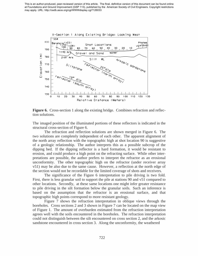
Figure 6. Cross-section 1 along the existing bridge. Combines refraction and reflec-tion solutions.

The imaged position of the illuminated portions of these reflectors is indicated in the structural cross-section of Figure 6.

The refraction and reflection solutions are shown merged in Figure 6. The two solutions are completely independent of each other. The apparent alignment of the north array reflection with the topographic high at shot location 90 is suggestive of a geologic relationship. The author interprets this as a possible subcrop of the dipping bed. If the dipping reflector is a hard formation, it would be resistant to erosion, and could produce a high point on the refracting surface. While other inter-pretations are possible, the author prefers to interpret the refractor as an erosional unconformity. The other topographic high on the refractor (under receiver array v51) may be also due to the same cause. However, a reflection at the north edge of the section would not be recordable for the limited coverage of shots and receivers.

The significance of the Figure 6 interpretation to pile driving is two fold. First, there is less granular soil to support the pile at stations 90 and v51 compared to other locations. Secondly, at these same locations one might infer greater resistance to pile driving in the silt formation below the granular soils. Such an inference is based on the assumption that the refractor is an erosional surface, and that topographic high points correspond to more resistant geology.

Figure 7 shows the refraction interpretation in oblique views through the boreholes. Cross sections 2 and 3 shown in Figure 7 can be located on the map view of Figure 1. The amount of overburden estimated from the refraction interpretation agrees well with the soils encountered in the boreholes. The refraction interpretation could not distinguish between the silt encountered on cross section 2, and the arkosic sandstone encountered in cross section 3. Along the unconformity, the weathered


(A) (B)

723

Figure 7. Cross sections that tie well control to the refraction profile at the south bank, (A), and at the north bank, (B). Figure 1 shows locations in map view.

arkosic sandstone appears to present about the same velocity as the silt and weathered siltstone. In any case, it would appear that the soil or rock below the overburden is suitable to support piles and the bridge foundation.

Down-hole GeophysicsThe down-hole survey was conducted in January, 2000, following the

completion of the drilling of the geotechnical borehole on the south bank. The down-hole survey served two purposes. First, the vertical component data provided p-velocity control for the overburden on the refraction interpretation. Second, sh-waves were analyzed for soil stiffness and damping properties. These properties can be useful in pile driving design (Fleming et al., 1985; Prakash and Sharma, 1990). The constitutive model is that of a Kelvin solid (spring in parallel with dashpot). Viscous damping results when the pore fluids and the soil frame are uncoupled.

The seismic source was a calibrated hammer capable of delivering 135 degree from the vertical impacts from two opposing directions. This source acquires both p- and sh-waves at the same time, and is described in Michaels (1998). Also described in that paper are the mathematical details on how stiffness and damping values may be determined from velocity dispersion and amplitude decay measure-ments of the propagating wave forms.

The down-hole geophone was a 3-component GeoStuff borehole phone with mechanical bow-spring clamp. The tool was lowered to the hole bottom and clamped by an electric motor driven mechanism. The clamped tool was dragged up hole to occupy 0.25 m spaced stations. At the surface, a 3-component reference phone was deployed to monitor source waveform and triggering consistency. Triggering was by contact closure. The recording instrument was an EGG Geomet-rics Strataview, sample interval of .00025 s and filters set at 0 and 1000 Hz.

The water table depth was determined with a moisture sensitive sounding tape and found to be at an elevation of +789.4 m (compared to +789.3 m mean river elevation earlier in the summer during the refraction work). Thus, the water table


0 0.05 0.10 Time (s)

DDH(W)-1 SH-Wave

0 0.02 0.04 0.06 Time (s)

DDH(W)-1 P-wave

Direct P-waveDirect SH-wave

724

divided the granular overburden into two zones. The vadose zone extended to a depth of about 2.9 m. Near saturated granular soil extended for about 6 meters, down to the top of the silt.

Data ProcessingThe vertical component data from both source directions were summed at

each depth station to provide a p-wave dominated record. The horizontal component data were subjected to hodogram analysis to determine the down-hole tool orienta-tion with respect to the source polarization. Then the down-hole data were mathematically rotated into alignment so that one component was parallel to the source azimuth. Opposing source polarizations were subtracted at each depth to provide an enhanced sh-wave record.

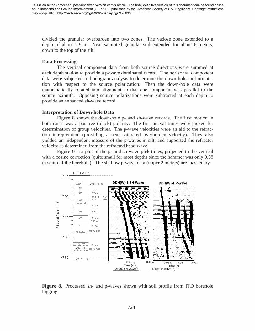
Interpretation of Down-hole DataFigure 8 shows the down-hole p- and sh-wave records. The first motion in

both cases was a positive (black) polarity. The first arrival times were picked for determination of group velocities. The p-wave velocities were an aid to the refrac-tion interpretation (providing a near saturated overburden velocity). They also yielded an independent measure of the p-waves in silt, and supported the refractor velocity as determined from the refracted head wave.

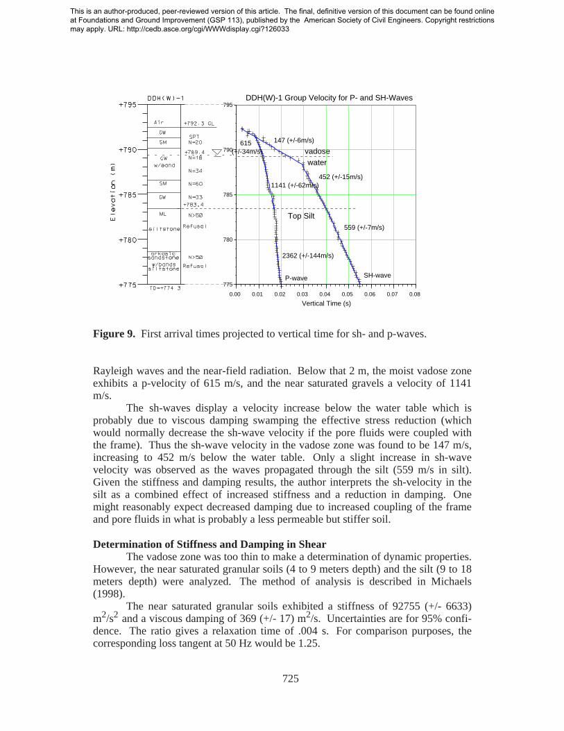
Figure 9 is a plot of the p- and sh-wave pick times, projected to the vertical with a cosine correction (quite small for most depths since the hammer was only 0.58 m south of the borehole). The shallow p-wave data (upper 2 meters) are masked by

Figure 8. Processed sh- and p-waves shown with soil profile from ITD borehole logging.


Top Silt

DDH(W)-1 Group Velocity for P- and SH-Waves

P-wave SH-wave

vadosewater

615(+/-34m/s)

0.00 0.01 0.02 0.03 0.04 0.05 0.06 0.07 0.08

775

780

785

790

795

Vertical Time (s)

559 (+/-7m/s)

2362 (+/-144m/s)

1141 (+/-62m/s) 452 (+/-15m/s)

147 (+/-6m/s)

725

Figure 9. First arrival times projected to vertical time for sh- and p-waves.

Rayleigh waves and the near-field radiation. Below that 2 m, the moist vadose zone exhibits a p-velocity of 615 m/s, and the near saturated gravels a velocity of 1141 m/s.

The sh-waves display a velocity increase below the water table which is probably due to viscous damping swamping the effective stress reduction (which would normally decrease the sh-wave velocity if the pore fluids were coupled with the frame). Thus the sh-wave velocity in the vadose zone was found to be 147 m/s, increasing to 452 m/s below the water table. Only a slight increase in sh-wave velocity was observed as the waves propagated through the silt (559 m/s in silt). Given the stiffness and damping results, the author interprets the sh-velocity in the silt as a combined effect of increased stiffness and a reduction in damping. One might reasonably expect decreased damping due to increased coupling of the frame and pore fluids in what is probably a less permeable but stiffer soil.

Determination of Stiffness and Damping in ShearThe vadose zone was too thin to make a determination of dynamic properties.

However, the near saturated granular soils (4 to 9 meters depth) and the silt (9 to 18 meters depth) were analyzed. The method of analysis is described in Michaels (1998).

The near saturated granular soils exhibited a stiffness of 92755 (+/- 6633) m2/s2 and a viscous damping of 369 (+/- 17) m2/s. Uncertainties are for 95% confi-dence. The ratio gives a relaxation time of .004 s. For comparison purposes, the corresponding loss tangent at 50 Hz would be 1.25.


(A) VELOCITY (B) ATTENUATION

Near Saturated Gravel and Sand 4<z<9 m

100200300400500600700800900

1000

Vel

ocity

(m

/s)

030 40 50 60 70 80 90 1000 10 20

Frequency (Hz)

⊕ ⊕ ⊕⊕

⊕ ⊕ ⊕ ⊕ ⊕⊕ ⊕ ⊕ ⊕ ⊕

⊕⊕

⊕

. 0.00.10.20.30.40.50.60.70.80.91.0

Atte

nuat

ion

(1/m

)

30 40 50 60 70 80 90 1000 10 20

Frequency (Hz)

.

⊕

⊕

⊕ ⊕ ⊕

⊕

⊕

⊕⊕

⊕⊕

⊕ ⊕ ⊕ ⊕ ⊕ ⊕

Solution: C1=92755 (+/-)6633 C2=369 (+/-)17

726

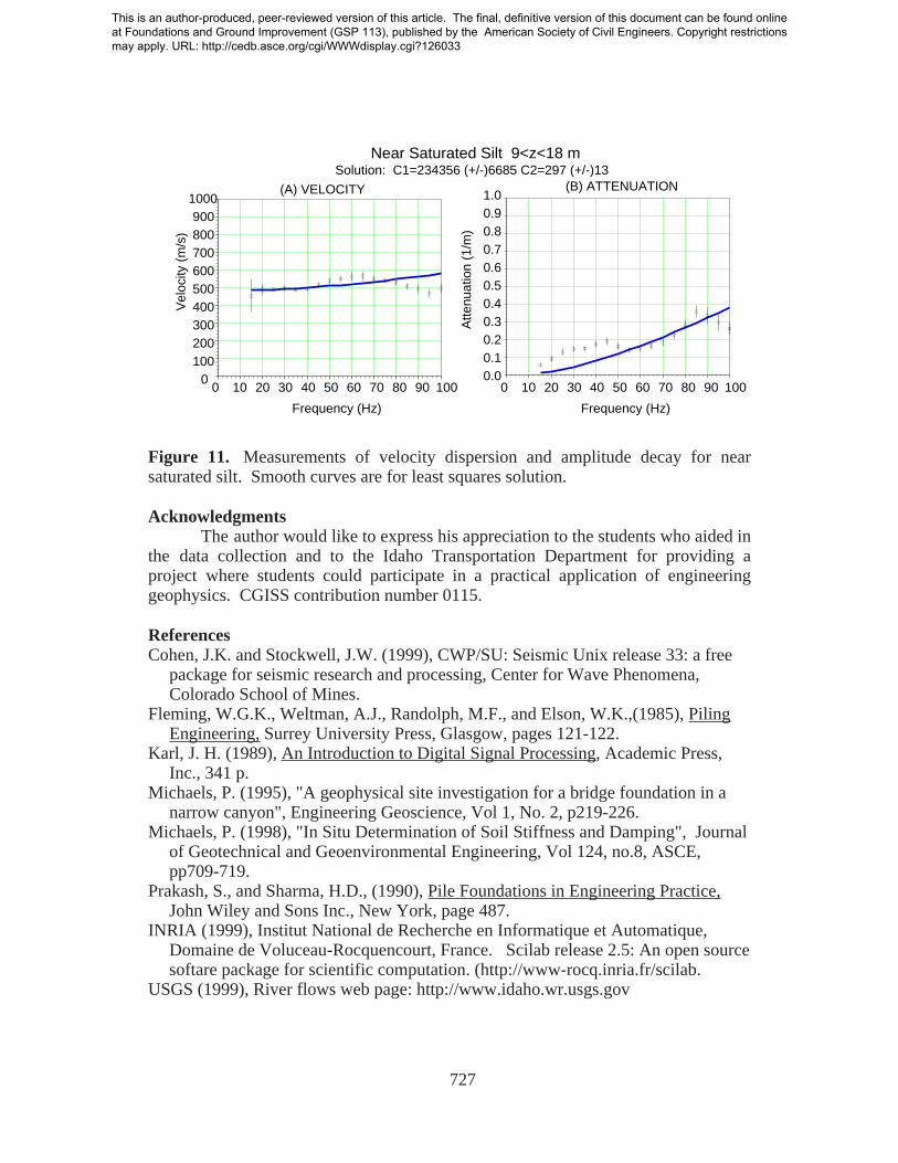
The silt exhibited an increase in stiffness and a decrease in damping. The stiffness value was found to be 234356 (+/-6685) m2/s2. The damping value was 297 (+/- 13) m2/s. The corresponding relaxation time is .0013 s and the loss tangent is 0.4 at 50 Hz.

Figure 10 shows the measured body wave dispersion and decay (corrected for geometrical spreading of the beam) in the near saturated granular soil. Figure 11 shows the same information for the silt zone. In comparing the two figures, one can see that the larger damping present in the gravels produces greater dispersion and more rapid amplitude decay. This is reasonable if the viscous coupling between frame and pore fluids is less in the gravels compared to the silt. Less coupling would be expected if the gravels are more permeable, permitting greater viscous interaction between the soil frame and pore water.

SummaryThe use of engineering geophysics provided an efficient way to derive a

geologic cross section to aid bridge engineers in their design of a replacement bridge. Interpretation of refraction and reflections provides an explanation of the lateral changes that occur between the north and south boreholes which terminated in significantly different materials (silt on the south bank, arkosic sandstone on the north bank). The lateral variations in geology appear to be due to erosional trunca-tion of dipping beds (19 to 25 degrees, down to the north). Locations likely to present thin overburden and resistant soil or rock have been identified in advance of pile driving.

Dynamic soil properties were determined that are relevant to pile driving and earthquake hazard evaluation. The granular soils were found to be less stiff than the silt, but possessing greater damping. This greater damping is explained as the result of greater permeability in the gravels which permits less viscous coupling between frame and pore fluids.

Figure 10. Measurements of velocity dispersion and amplitude decay for near saturated granular soils. Smooth curves are for least squares solution.


(A) VELOCITY (B) ATTENUATION

Near Saturated Silt 9<z<18 m

100200300400500600700800900

1000V

eloc

ity (

m/s

)

030 40 50 60 70 80 90 1000 10 20

Frequency (Hz)

.

⊕⊕ ⊕ ⊕ ⊕ ⊕

⊕⊕ ⊕ ⊕ ⊕ ⊕ ⊕ ⊕

⊕ ⊕⊕

⊕

0.00.10.20.30.40.50.60.70.80.91.0

Atte

nuat

ion

(1/m

)

30 40 50 60 70 80 90 1000 10 20

Frequency (Hz)

.

⊕⊕

⊕ ⊕ ⊕⊕

⊕⊕

⊕ ⊕ ⊕⊕

⊕

⊕

⊕⊕

⊕⊕

Solution: C1=234356 (+/-)6685 C2=297 (+/-)13

727

Figure 11. Measurements of velocity dispersion and amplitude decay for near saturated silt. Smooth curves are for least squares solution.

AcknowledgmentsThe author would like to express his appreciation to the students who aided in

the data collection and to the Idaho Transportation Department for providing a project where students could participate in a practical application of engineering geophysics. CGISS contribution number 0115.

ReferencesCohen, J.K. and Stockwell, J.W. (1999), CWP/SU: Seismic Unix release 33: a free

package for seismic research and processing, Center for Wave Phenomena, Colorado School of Mines.

Fleming, W.G.K., Weltman, A.J., Randolph, M.F., and Elson, W.K.,(1985), Piling Engineering, Surrey University Press, Glasgow, pages 121-122.

Karl, J. H. (1989), An Introduction to Digital Signal Processing, Academic Press, Inc., 341 p.

Michaels, P. (1995), "A geophysical site investigation for a bridge foundation in a narrow canyon", Engineering Geoscience, Vol 1, No. 2, p219-226.

Michaels, P. (1998), "In Situ Determination of Soil Stiffness and Damping", Journal of Geotechnical and Geoenvironmental Engineering, Vol 124, no.8, ASCE, pp709-719.

Prakash, S., and Sharma, H.D., (1990), Pile Foundations in Engineering Practice, John Wiley and Sons Inc., New York, page 487.

INRIA (1999), Institut National de Recherche en Informatique et Automatique, Domaine de Voluceau-Rocquencourt, France. Scilab release 2.5: An open source softare package for scientific computation. (http://www-rocq.inria.fr/scilab.

USGS (1999), River flows web page: http://www.idaho.wr.usgs.gov


Documents

Use of Engineering Geophysics to Investigate a Site for a