Use of AMI Meters in the Process of Low Voltage Grid …actaenergetica.org/uploads/oryginal/2/3/e061aca4_Dobrzynski_Use_of... · The objective of the grant was to investigate the

58

Use of AMI Meters in the Process of Low Voltage Grid Optimization

AuthorsKrzysztof DobrzyńskiZbigniew LubośnyJacek KlucznikSławomir NoskeDominik Falkowski

Keywordslow voltage grid, grid monitoring and control, optimization

AbstractThis is a report of a project involving, inter alia, low voltage grid performance optimization with data from AMI meters. The study was supported with a European UPGRID grant, and executed by a consortium of companies from seven European countries, including Poland.

DOI: 10.12736/issn.2300-3022.2017305

Received: 06.02.2017Accepted: 27.06.2017Available online: 30.09.2017

1. IntroductionThe knowledge of the Distribution System Operator concerning the actual state of the low voltage grid is currently very limited. This means that the distribution operator does not have suffi-cient information about the current voltages and loads of grid components in the low voltage grid, or it is merely the residual knowledge of a selected test area of the grid, as is the case with the Hel Peninsula, for example. In the case of LV grid failures, basically the only source of feedback are the blackout notices from customers conveyed by phone or via the Internet. Similarly,

the operator doesn’t know much about the power quality, since it is analysed upon customer complaint only. Following the large-scale deployment of AMI infrastructure, operators have been investigating the suitability of AMI meters for purposes other than just metering and billing energy consumption. AMI meters, depending on the model, can record different electrical parameters, such as instantaneous voltage and power values, and pre-defined events (e.g. voltage drop). The combination of these features with the ability of AMI meters to remotely retrieve measurements has prompted researchers to look for additional

Fig. 1. General structure of DMS system. MDM – Meter Data Management; NCM – Network Control and Management; OMS – Outage Management System; NA – Network Analysis; MDG – Meter Data Gateway; CBP – Central Database; SCADA – Supervisory Control and Data Acquisition

K. Dobrzyński et al. | Acta Energetica 3/32 (2017) | 58–63

59

areas where this infrastructure may be used. Verifying the new applications of AMI infrastructure is a complex undertaking that on the one hand involves significant enterprise resources, and on the other hand requires third-party support for tasks outside the operator’s core business, e.g. development of new software.At the beginning of 2015, ENERGA-OPERATOR SA, Gdańsk University of Technology, Institute of Power Engineering, and Atende SA commenced cooperation in the implementation of a project financed by an UPGRID European grant under the Horizon 2020 program [4]. Besides the Polish partners, the project participants include 15 more from 7 different European countries. The grant was aimed at investigating the feasibility and viability of a remote monitoring and control system for low and medium voltage grids. However, the operator is allowed a certain flexibility with regard to the choice of issues that they may wish to address as long as they remain defined within certain topics. The distri-bution operator in a given country specifies which issues will be addressed. This is justified by the differences between operators, both in terms of technology and the experience already gained. The Polish operator focused on issues related to the low voltage grid.This paper reports selected issues addressed under the grant by the Polish partners [1], including:• LV grid monitoring and control• power flow calculation in LV grid• LV grid state estimation• load and generation forecasting in LV grids• optimization of LV grid division points• MV/LV transformer temperature forecasting• optimum choice of transformer for MV/LV substation• fault location.In the project, the above-mentioned issues constitute the inde-pendently considered functionalities included in the developed

Distribution Management System (DMS). The general structure of this system is shown in Fig. 1.

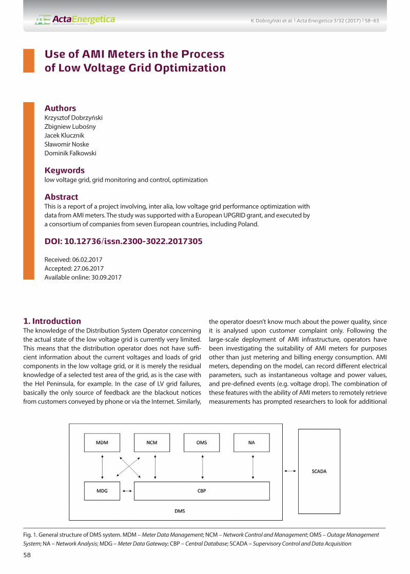
2. The low and medium voltage grid test areaThe objective of the grant was to investigate the relevant issues in an real distribution grid. Therefore, a definite demonstration area of the medium and low voltage grids, located within Gdynia city districts, was identified: Witomino, Działki Leśne and Chwarzno (Fig. 2). This area consists of:• 33.71 km of medium voltage cable lines• 90.75 km of low voltage cable lines• 26.68 km of low voltage overhead lines• 54 indoor MV/LV transformer substations, which supply

300 low voltage circuits.All MV/LV substations in the demonstration area were equipped with AMI infrastructure, including: a concentrator that collects measurements from customer meters and a balancing meter located on LV side of the MV/LV transformers. As part of the project, selected MV/LV substations were upgraded to provide adequate levels of grid monitoring and control. For example, in three selected substations, currents were measured and fuses inspected in each LV circuit.

3. Functionalities planned in LV gridWithin the grant framework, many low voltage grid function-alities were provided for. The following is a brief description of these functionalities with selected issues and/or constraints that affect the current implementation.

3.1. LV grid monitoring and controlThe LV grid is monitored and controlled by Polish distribution operators, basically only in pilot areas where selected solutions are being tested. In this case, in principle for the first time, the

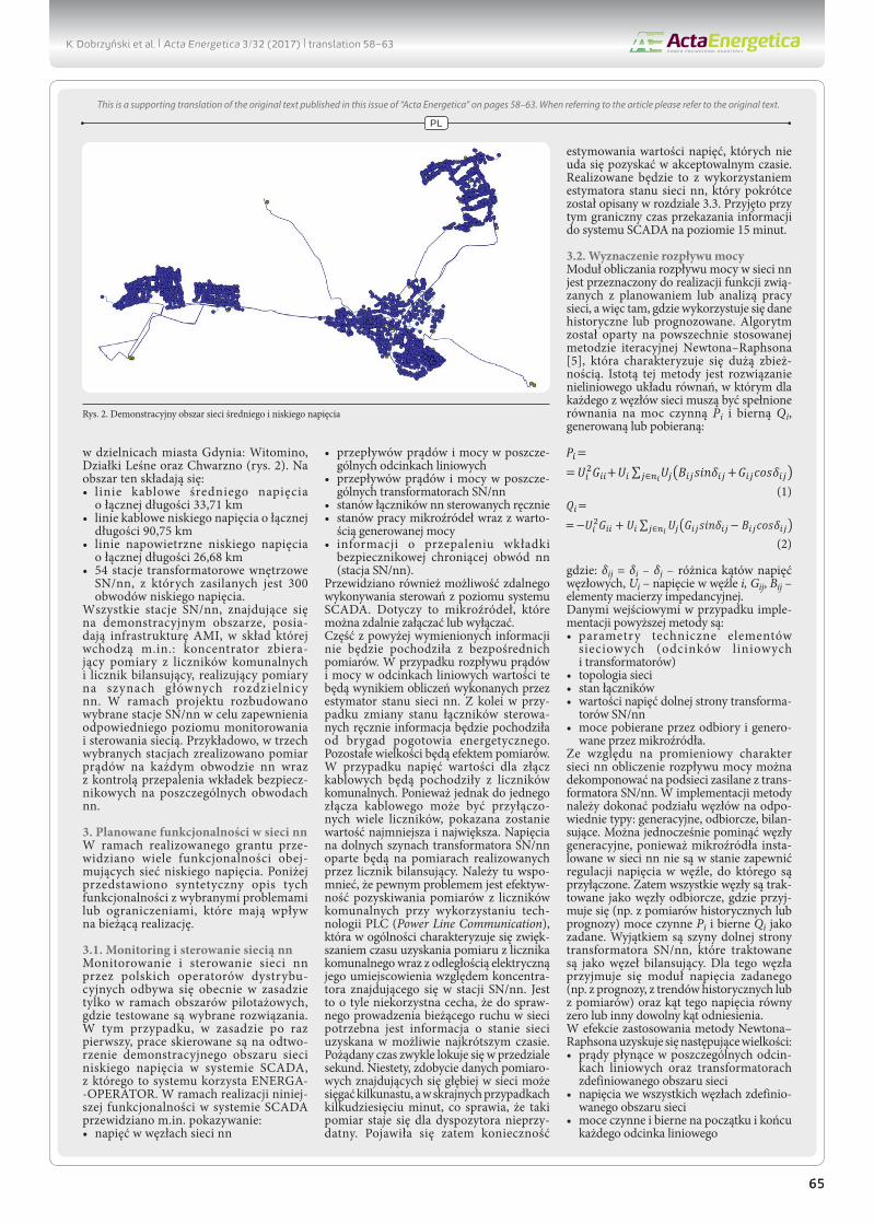
Fig. 2. Demonstration area of medium and low voltage grids


60

research effort is aimed at the make a model of the LV grid’s demonstration area in the SCADA system, which is in place at ENERGA-OPERATOR. As part of the implementation of this functionality in the SCADA system, the following features were monitored:• LV grid node voltages• current and power flows in line sections• current and power flows in MV/LV transformers• manual LV switch statuses• micro-source operational status, incl. measure output power• information on blown fuses in the LV feeders (MV/LV

substation). Also, the option of remote control from the SCADA system was provided for. This applies to micro-sources that can be remotely turned on or off.Some of the above information will not come from direct measurements. The current and power flows in line sections will be calculated by the LV grid state estimator. On the other hand, a change in the status of a manually controlled switch will be identified and notified by an Electrical Emergency Service field crew. The other values will be measured. Cable cabinet volt-ages will be taken from customer meters. However, since there may be multiple meters connected to one cable cabinet, the minimum and maximum value will be shown. Voltages on the LV buses of the MV/LV transformers will be measured by a balancing meter. It is worth mentioning that one problem is the efficiency of measurement acquisition from customer meters using PLC (Power Line Communication) technology, which in general, increases the time of measurement retrieval from customer meters along with the electrical distance of its location relative to the concentrator located in the MV/LV substation. This is unfortu-nate due to the fact that for the efficient management of current grid operation, information is needed concerning the grid state and should be acquired as soon as possible. The desired time is usually counted in seconds. Unfortunately, the acquisition of data measured deeper in the grid can take a dozen or so, and in extreme cases a few dozen, minutes, which makes this measure-ment unsuitable for the operator. Therefore, the need arose to estimate the voltages that cannot be acquired in an acceptable time. This will be accomplished by using the LV grid condition estimator, which has been briefly described in point 3.3. In this case, the time limit for transferring information to the SCADA system was 15 minutes.

3.2. Power flowsThe LV grid power flow calculation module is designed to perform the functions of grid operation planning or analysis, which is where historical or forecast data are used. The algorithm was based on the commonly used Newton-Raphson iteration method [5], which features high convergence. The essence of this method is the solution of a non-linear system of equations in which the active Pi and reactive Qi power shall be fulfilled in each network node:

(1)

(2)

where: δij = δi – δj – difference between nodal voltage angles, Ui – voltage in node i, Gij, Bij – impedance matrix elements.The input data for the implementation of the above method are:• technical parameters of grid components (line sections and

transformers)• grid topology• switches state• LV side voltages of MV/LV transformers• load and generation powers of micro-sources.Due to the radial configuration of the LV grid, the power flow calculation can be split into sub-grids supplied from MV/LV trans-formers. In the method, nodes should be divided into genera-tion, load, and balancing types. At the same time, the generation nodes may be ignored, because the micro sources installed in the LV grid are not capable of voltage regulation. Thus, all nodes are treated as loads, with their active and reactive powers Pi and Qi assumed (e.g. from historical measurements or forecasts) as preset. The exception is the LV side buses of the MV/LV trans-former, which are treated as balancing node. For this node, the preset voltage module is assumed (e.g. from forecast, historical trends or measurements) and the angle of that voltage equals zero or any other reference angle.As a result of the Newton-Raphson method application, the following values are obtained:• currents in line sections and transformers in a defined grid

area• voltages in all nodes in a defined grid area• active and reactive powers at the beginning and end of each

line section• active and reactive power flows through transformers• active and reactive power losses in all line sections.

3.3. LV grid status estimationThe main information of interest to the operator while providing current control of the grid operation, are node voltages and loads of individual line sections and transformers. As mentioned earlier, in the case of a low voltage grid, at present, the oper-ator has no current knowledge about its actual state. With the help of AMI infrastructure, information may be obtained, but with certain limitations. The main limitation is the efficiency of measurement acquisition from customer meters. For this reason, the power flow module cannot be used and the grid state esti-mator should be used, which will fill missing measurements. Currently, based on completed analyses, it is predicted that in the assumed 15-min. time interval measurements could be acquired from most customer meters, but not all. The above information makes it necessary to apply a solution which, based on incom-plete data, will provide a reliable state of LV grid.Input data for the algorithm basically coincides with those needed in the power flow calculation module (point 3.2). In this case, no load and generation powers are needed.Additionally, the following are required:• voltage measurements in selected customer meters• energy measurements in balancing meters.


61

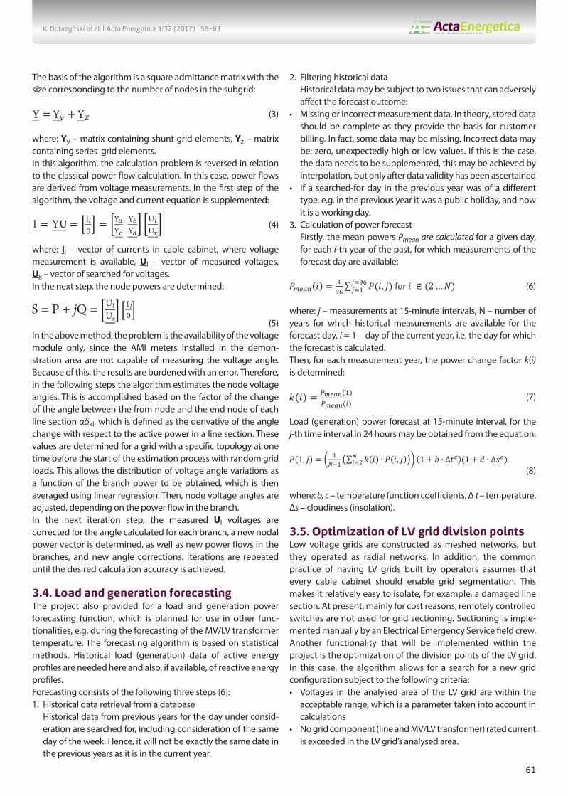
The basis of the algorithm is a square admittance matrix with the size corresponding to the number of nodes in the subgrid:

(3)

where: Yy – matrix containing shunt grid elements, Yz – matrix containing series grid elements.In this algorithm, the calculation problem is reversed in relation to the classical power flow calculation. In this case, power flows are derived from voltage measurements. In the first step of the algorithm, the voltage and current equation is supplemented:

(4)

where: Il – vector of currents in cable cabinet, where voltage measurement is available, Ul – vector of measured voltages, Ux – vector of searched for voltages.In the next step, the node powers are determined:

(5)In the above method, the problem is the availability of the voltage module only, since the AMI meters installed in the demon-stration area are not capable of measuring the voltage angle. Because of this, the results are burdened with an error. Therefore, in the following steps the algorithm estimates the node voltage angles. This is accomplished based on the factor of the change of the angle between the from node and the end node of each line section αδkl, which is defined as the derivative of the angle change with respect to the active power in a line section. These values are determined for a grid with a specific topology at one time before the start of the estimation process with random grid loads. This allows the distribution of voltage angle variations as a function of the branch power to be obtained, which is then averaged using linear regression. Then, node voltage angles are adjusted, depending on the power flow in the branch.In the next iteration step, the measured Ul voltages are corrected for the angle calculated for each branch, a new nodal power vector is determined, as well as new power flows in the branches, and new angle corrections. Iterations are repeated until the desired calculation accuracy is achieved.

3.4. Load and generation forecastingThe project also provided for a load and generation power forecasting function, which is planned for use in other func-tionalities, e.g. during the forecasting of the MV/LV transformer temperature. The forecasting algorithm is based on statistical methods. Historical load (generation) data of active energy profiles are needed here and also, if available, of reactive energy profiles.Forecasting consists of the following three steps [6]:1. Historical data retrieval from a database Historical data from previous years for the day under consid-

eration are searched for, including consideration of the same day of the week. Hence, it will not be exactly the same date in the previous years as it is in the current year.

2. Filtering historical data Historical data may be subject to two issues that can adversely

affect the forecast outcome:• Missing or incorrect measurement data. In theory, stored data

should be complete as they provide the basis for customer billing. In fact, some data may be missing. Incorrect data may be: zero, unexpectedly high or low values. If this is the case, the data needs to be supplemented, this may be achieved by interpolation, but only after data validity has been ascertained

• If a searched-for day in the previous year was of a different type, e.g. in the previous year it was a public holiday, and now it is a working day.

3. Calculation of power forecast Firstly, the mean powers Pmean are calculated for a given day,

for each i-th year of the past, for which measurements of the forecast day are available:

(6)

where: j – measurements at 15-minute intervals, N – number of years for which historical measurements are available for the forecast day, i = 1 – day of the current year, i.e. the day for which the forecast is calculated.Then, for each measurement year, the power change factor k(i) is determined:

(7)

Load (generation) power forecast at 15-minute interval, for the j-th time interval in 24 hours may be obtained from the equation:

(8)

where: b, c – temperature function coefficients, Δ t – temperature, Δs – cloudiness (insolation).

3.5. Optimization of LV grid division pointsLow voltage grids are constructed as meshed networks, but they operated as radial networks. In addition, the common practice of having LV grids built by operators assumes that every cable cabinet should enable grid segmentation. This makes it relatively easy to isolate, for example, a damaged line section. At present, mainly for cost reasons, remotely controlled switches are not used for grid sectioning. Sectioning is imple-mented manually by an Electrical Emergency Service field crew.Another functionality that will be implemented within the project is the optimization of the division points of the LV grid. In this case, the algorithm allows for a search for a new grid configuration subject to the following criteria:• Voltages in the analysed area of the LV grid are within the

acceptable range, which is a parameter taken into account in calculations

• No grid component (line and MV/LV transformer) rated current is exceeded in the LV grid’s analysed area.


62

A variety of goal functions may be optimized here, including:• elimination of overloads in an LV grid area• elimination of overvoltages in an LV grid area• search for a new division points because of the need to

deenergize a grid component or area, e.g. for the failure removal or performing a scheduled works

• minimizing technical losses in an LV grid area.The algorithm performs calculations for the actual configura-tion of the defined LV grid area, taking into account the load forecasts over a specified time and at a defined time interval. Then new grid configurations are searched for that meet the criteria are set out as a ranking list.

3.6. MV/LV transformer temperature forecastingAt MV/LV substations, the power flows through transformers are measured every 15 minutes by a balancing meter. These measurements are sent to the AMI system and stored there, so that the transformer load history is available. Based on the measured powers, the transformer temperature in its hottest place can be approximately estimated. The temperature determination is based on standards PN IEC 60354 [2] and PN EN 60076-2 [3].Based on the transformer load history, with the forecasting function (described in section 3.4) the transformer load may be predicted, e.g. for the next 12 hours. However, the predic-tion is only possible if the subgrid supplied from this trans-former has not changed in relation to the measurements from previous years. If this condition is not met, then the forecast made for each customer meter currently fed from the trans-former should be used. This approach is also valid for cases where the grid is reconfigured, for example, under the optimi-zation of division points, and it should be verified whether the new configuration would result in the transformer’s overload in the perspective of its daily load.

3.7. Optimum choice of transformer for MV/LV substationIn general, the low voltage grid, more than the other grids, is subject to constant changes, especially in load power, and soon also with regard to micro-source. On the one hand, this is due to the progressive increase in the energy consuming of households, along with economic development growth. On the other hand, it is due to the emergence of new energy consumption points with progresses in urban development and tenant changes in existing buildings. Taking all of this into account, the MV/LV transformer load curves do not neces-sarily replicate every year and may change over time. This may in turn lead to the ineffective use of individual distribution transformers and necessitate their replacement.Economic criteria were proposed in the project for trans-former selection for MV/LV substations, with consideration of the costs incurred for the technical losses of transformers and their replacement costs. It is assumed here that the

transformer is not purchased and comes from the distribution operator’s stockpile. In the first step, the algorithm, based on the forecast transformer load and voltages, calculates energy losses, no-load and load, for the entire year. Then the trans-former replacement cost is calculated, and includes: disas-sembly, assembly and transport. The decision to replace the transformer is based on the replacement cost comparison with losses throughout the transformer’s useful life.

3.8. Fault locationPresently, operators locate failures in LV grids based on the phone calls or internet reports of consumers. The project analyses a function that uses AMI infrastructure to assist the operator in LV grid fault detection.AMI meters can report voltage loss to the concentrator at the MV/LV substation. The limitation here is that a single-phase meter is able to send such information only after the supply voltage has been restored. Whereas a 3-phase meter can send the information immediately, but only when power supply failure occurs in one or two phases.Another way to deduce the occurrence of an LV grid failure is to analyse the communication between the concentrator and customer meters. Normally, the metering data from the customer meters are transferred to the concentrator in MV/LV substations in cycles. Communication between the meters and concentrator is continuously monitored by the concen-trator. This means that the concentrator knows immediately which meter has answered the measurement request. The absence of a customer meter response to the concentrator’s query within a given time may be a premise for concluding that there is a failure in the grid. If there is no response, then the next step is to verify the list of the concentrators that have communicated with this meter in the past, and to see if the data was sent within the specified time period. The absence of meter communication with other concentrators may indi-cate a failure. The meters’ concentration, especially in urban subgrids, is also included in the algorithm. For example, in a multi-family house, the lack of response from a single customer meter may indicate the activation of circuit-breaker for the given meter. However, if many meters do not respond, then a failure is highly likely.

4. SummaryThe existing AMI infrastructure prompts distribution opera-tors to take action aimed at benefiting from the opportunities offered by this infrastructure, other than just energy billing. ENERGA-OPERATOR SA together with partners, within the framework of European UPGRID grant, implements LV grid monitoring and control solutions in a demonstration area. The aim is to gain knowledge and experience in the use of AMI infrastructure.


63

REFERENCES

1. Z. Lubośny et al., “Real proven solutions to enable active demand and distributed generation flexible integration, through a fully controllable LOW Voltage and medium voltage distribution grid. Demonstration 4 in real user environment: ENERGA – Poland. System Design, under grant 646531 — UPGRID — H2020-LCE-2014-2015/H2020-LCE-2014-3”, Gdańsk 2016.

2. PN IEC 60354: 1999, “Loading guide for oil-immersed power transformers”.

3. PN EN 60076-2: 2011, “Temperature rise for oil-immersed transformers”.

4. www.upgrid.eu.5. Z. Kremens, M. Sobierajski, “Analiza systemów elektroenergetyc-

znych” [Analysis of power systems], WNT 1996.6. H. Dobrzańska et al., „Prognozowanie w elektroenergetyce.

Zagadnienia wybrane” [Forecasting in power engineering. Selected issues] Częstochowa University of Technology Publishers, Częstochowa, 2002.

Krzysztof DobrzyńskiGdańsk University of Technology

e-mail: [email protected]

Graduated from the Faculty of Electrical Engineering at Warsaw University of Technology (1999). He earned his Ph.D. at the Faculty of Electrical and Control Engineering

at Gdańsk University of Technology (2012). An assistant professor at the Power Engineering Department of Gdańsk University of Technology. His areas of interest

include interoperation of distributed generation sources within the power system, mathematical modelling, power system control, and intelligent systems in buildings.

Zbigniew LubośnyGdańsk University of Technology


Graduated from Gdańsk University of Technology. A professor of engineering since 2004. Currently an associate professor at Gdańsk University of Technology. His areas

of interest include mathematical modelling, power system stability, power system control, the use of artificial intelligence applications in power system control, and

the modelling and control of wind turbines. Editor in Chief of Acta Energetica.

Jacek KlucznikGdańsk University of Technology


He graduated from the Faculty of Electrical and Control Engineering at Gdańsk University of Technology (1999). Five years later he obtained his Ph.D. An assistant

professor at the Power Engineering Department of his alma mater. His areas of interest include control systems for generators and turbines, wind power generation,

and power system automatic protections.

Sławomir NoskeENERGA-OPERATOR SA


Graduated from the Faculty of Electrical Engineering at Poznan University of Technology, where he obtained his doctorate in engineering. Graduated from MBA

studies. Professionally involved with the distribution of energy. Now in R&D at ENERGA-OPERATOR SA. At the centre of his interests are: smart grids, diagnostics in cable

grids, grid asset management. CIGRE member and Polish representative in the Study Committee of B1 Cables.

Dominik FalkowskiENERGA-OPERATOR SA


PhD student at Gdańsk University of Technology, working at ENERGA-OPERATOR Innovation Department. During his studies he was awarded a distinction in the

ENERGA SA contest for a project on the impact of investment until 2025 in generation capacity and transmission and distribution grids on the load carrying capacities

of the nodes and lines in the ENERGA SA operating area. Professional interests: smart grids, power system development and new energy transmission and storage

technologies.


64

PL

Wykorzystanie liczników AMI w procesie optymalizacji pracy sieci niskiego napięcia

AutorzyKrzysztof Dobrzyński Zbigniew Lubośny Jacek Klucznik Sławomir Noske Dominik Falkowski

Słowa kluczowesieć niskiego napięcia, monitoring i sterowanie sieci, optymalizacja

StreszczeniePrezentowany jest opis projektu dotyczącego m.in. optymalizacji pracy sieci niskiego napięcia przy wykorzystaniu danych z licz-ników AMI. Prace były prowadzone w ramach europejskiego grantu UPGRID, realizowanego przez konsorcjum firm z siedmiu państw europejskich, w tym również z Polski.

Data wpływu do redakcji: 06.02.2017Data akceptacji artykułu: 27.06.2017Data publikacji online: 30.09.2017

1. WstępWiedza operatora dystrybucyjnego na temat aktualnego stanu pracy sieci niskiego napięcia jest obecnie bardzo skromna. Oznacza to, że operator dystrybucyjny nie dysponuje informacjami na temat aktual-nych napięć i obciążeń elementów siecio-wych w sieci niskiego napięcia albo jest to wiedza szczątkowa, obejmująca tylko wybrany, testowy obszar sieci, tak jak ma to miejsce np. na Półwyspie Helskim. W przypadku wykrywania awarii w sieci nn w zasadzie jedynym źródłem są infor-macje o zaniku zasilania dostarczane przez klientów telefonicznie lub drogą interne-tową. Podobnie sytuacja wygląda z wiedzą operatora na temat jakości energii elek-trycznej, gdzie ewentualne analizy podej-mowane są po uprzednich reklamacjach ze strony klientów. Wykorzystanie infra-struktury AMI na szeroką skalę sprawiło, że obecnie operatorzy badają możliwości wykorzystania liczników AMI do innych zadań niż tylko rozliczeń rzeczywistego zużycia energii elektrycznej. Liczniki AMI, w zależności od modelu, mają zdolność reje-strowania różnych wielkości elektrycznych, takich jak np.: chwilowe wartości napięć, chwilowe wartości mocy, zdefiniowane zdarzenia (np. chwilowe obniżenie napięcia). Połączenie wymienionych własności licz-ników AMI z możliwością zdalnego pobie-rania pomiarów sprawia, że rozważane są kolejne obszary, w których można wyko-rzystać tę infrastrukturę. Zweryfikowanie nowych zastosowań infrastruktury AMI jest złożonym przedsięwzięciem, w którym z jednej strony należy zaangażować wiele zasobów przedsiębiorstwa, a z drugiej strony potrzebne jest wsparcie firm zewnętrz-nych, potrafiących zrealizować zagadnienia niebędące domeną operatora, np. stronę programistyczną. Z początkiem 2015 roku ENERGA- -OPERATOR SA, Politechnika Gdańska,

Instytut Elektroenergetyki oraz Atende SA rozpoczęły współudział w realizacji grantu europejskiego o akronimie UPGRID, realizowanego w ramach programu Horyzont 2020 [4]. W grancie tym, oprócz polskich partnerów, uczestniczy jeszcze 15 innych z 7 różnych państw europejskich. W swoim założeniu grant ten dotyczy realizowalności systemu zdalnego moni-torowania i sterowania siecią niskiego i średniego napięcia. Przy czym dopusz-czona jest tu pewna elastyczność wyboru przez operatorów realizowanych zagad-nień, zdefiniowanych w ramach przyję-tych tematyk. Operator dystrybucyjny w danym kraju precyzuje, które zagad-nienia realizuje. Jest to uzasadnione różni-cami pomiędzy operatorami, zarówno w sferze technologicznej, jak i już zdoby-tych doświadczeń. Polski operator skon-centrował się na zagadnieniach związa-nych z siecią niskiego napięcia.Niniejszy referat przedstawia wybrane zagadnienia realizowane w ramach przed-miotowego grantu przez polskich part-nerów [1], a są to m.in.:

• monitorowanie i sterowanie siecią nn• obliczanie rozpływu mocy w sieci nn• estymacja stanu sieci nn• prognozowanie obciążenia i generacji

w sieci nn• optymalizacja punktów podziału sieci nn• prognozowanie temperatury transforma-

tora SN/nn• wybór optymalnego transformatora dla

stacji SN/nn• lokalizacja awarii.Powyżej wymienione zagadnienia stanowią w projekcie niezależnie rozważane funkcjo-nalności wchodzące w skład opracowanego systemu DMS (Distribution Management System). Ogólną strukturę tego systemu przedstawiono na rys. 1.

2. Charakterystyka obszaru testowego sieci niskiego i średniego napięciaIdea przedmiotowego grantu polega na sprawdzeniu realizowanych zagad-nień w rzeczywistej sieci dystrybucyjnej. Do analiz zdefiniowano zatem okre-ślony demonstracyjny obszar sieci śred-niego i niskiego napięcia, znajdujący się

Rys. 1. Ogólna struktura systemu DMS. MDM – Meter Data Management; NCM – Network Control and Management; OMS – Outage Management System; NA – Network Analysis; MDG – Meter Data Gateway; CBP – Central Database; SCADA – Supervisory Control and Data Acquisition

K. Dobrzyński et al. | Acta Energetica 3/32 (2017) | translation 58–63

This is a supporting translation of the original text published in this issue of “Acta Energetica” on pages 58–63. When referring to the article please refer to the original text.

6565

PL

w dzielnicach miasta Gdynia: Witomino, Działki Leśne oraz Chwarzno (rys. 2). Na obszar ten składają się:• linie kablowe średniego napięcia

o łącznej długości 33,71 km• linie kablowe niskiego napięcia o łącznej

długości 90,75 km• linie napowietrzne niskiego napięcia

o łącznej długości 26,68 km• 54 stacje transformatorowe wnętrzowe

SN/nn, z których zasilanych jest 300 obwodów niskiego napięcia.

Wszystkie stacje SN/nn, znajdujące się na demonstracyjnym obszarze, posia-dają infrastrukturę AMI, w skład której wchodzą m.in.: koncentrator zbiera-jący pomiary z liczników komunalnych i licznik bilansujący, realizujący pomiary na szynach głównych rozdzielnicy nn. W ramach projektu rozbudowano wybrane stacje SN/nn w celu zapewnienia odpowiedniego poziomu monitorowania i sterowania siecią. Przykładowo, w trzech wybranych stacjach zrealizowano pomiar prądów na każdym obwodzie nn wraz z kontrolą przepalenia wkładek bezpiecz-nikowych na poszczególnych obwodach nn.

3. Planowane funkcjonalności w sieci nnW ramach realizowanego grantu prze-widziano wiele funkcjonalności obej-mujących sieć niskiego napięcia. Poniżej przedstawiono syntetyczny opis tych funkcjonalności z wybranymi problemami lub ograniczeniami, które mają wpływ na bieżącą realizację.

3.1. Monitoring i sterowanie siecią nnMonitorowanie i sterowanie sieci nn przez polskich operatorów dystrybu-cyjnych odbywa się obecnie w zasadzie tylko w ramach obszarów pilotażowych, gdzie testowane są wybrane rozwiązania. W tym przypadku, w zasadzie po raz pierwszy, prace skierowane są na odtwo-rzenie demonstracyjnego obszaru sieci niskiego napięcia w systemie SCADA, z którego to systemu korzysta ENERGA- -OPERATOR. W ramach realizacji niniej-szej funkcjonalności w systemie SCADA przewidziano m.in. pokazywanie:• napięć w węzłach sieci nn

• przepływów prądów i mocy w poszcze-gólnych odcinkach liniowych

• przepływów prądów i mocy w poszcze-gólnych transformatorach SN/nn

• stanów łączników nn sterowanych ręcznie• stanów pracy mikroźródeł wraz z warto-

ścią generowanej mocy• informacji o przepaleniu wkładki

bezpiecznikowej chroniącej obwód nn (stacja SN/nn).

Przewidziano również możliwość zdalnego wykonywania sterowań z poziomu systemu SCADA. Dotyczy to mikroźródeł, które można zdalnie załączać lub wyłączać.Część z powyżej wymienionych informacji nie będzie pochodziła z bezpośrednich pomiarów. W przypadku rozpływu prądów i mocy w odcinkach liniowych wartości te będą wynikiem obliczeń wykonanych przez estymator stanu sieci nn. Z kolei w przy-padku zmiany stanu łączników sterowa-nych ręcznie informacja będzie pochodziła od brygad pogotowia energetycznego. Pozostałe wielkości będą efektem pomiarów. W przypadku napięć wartości dla złącz kablowych będą pochodziły z liczników komunalnych. Ponieważ jednak do jednego złącza kablowego może być przyłączo-nych wiele liczników, pokazana zostanie wartość najmniejsza i największa. Napięcia na dolnych szynach transformatora SN/nn oparte będą na pomiarach realizowanych przez licznik bilansujący. Należy tu wspo-mnieć, że pewnym problemem jest efektyw-ność pozyskiwania pomiarów z liczników komunalnych przy wykorzystaniu tech-nologii PLC (Power Line Communication), która w ogólności charakteryzuje się zwięk-szaniem czasu uzyskania pomiaru z licznika komunalnego wraz z odległością elektryczną jego umiejscowienia względem koncentra-tora znajdującego się w stacji SN/nn. Jest to o tyle niekorzystna cecha, że do spraw-nego prowadzenia bieżącego ruchu w sieci potrzebna jest informacja o stanie sieci uzyskana w możliwie najkrótszym czasie. Pożądany czas zwykle lokuje się w przedziale sekund. Niestety, zdobycie danych pomiaro-wych znajdujących się głębiej w sieci może sięgać kilkunastu, a w skrajnych przypadkach kilkudziesięciu minut, co sprawia, że taki pomiar staje się dla dyspozytora nieprzy-datny. Pojawiła się zatem konieczność

estymowania wartości napięć, których nie uda się pozyskać w akceptowalnym czasie. Realizowane będzie to z wykorzystaniem estymatora stanu sieci nn, który pokrótce został opisany w rozdziale 3.3. Przyjęto przy tym graniczny czas przekazania informacji do systemu SCADA na poziomie 15 minut.

3.2. Wyznaczenie rozpływu mocyModuł obliczania rozpływu mocy w sieci nn jest przeznaczony do realizacji funkcji zwią-zanych z planowaniem lub analizą pracy sieci, a więc tam, gdzie wykorzystuje się dane historyczne lub prognozowane. Algorytm został oparty na powszechnie stosowanej metodzie iteracyjnej Newtona–Raphsona [5], która charakteryzuje się dużą zbież-nością. Istotą tej metody jest rozwiązanie nieliniowego układu równań, w którym dla każdego z węzłów sieci muszą być spełnione równania na moc czynną Pi i bierną Qi, generowaną lub pobieraną:

(1)

(2)

gdzie: δij = δi – δj – różnica kątów napięć węzłowych, Ui – napięcie w węźle i, Gij, Bij – elementy macierzy impedancyjnej.Danymi wejściowymi w przypadku imple-mentacji powyższej metody są:• parametry techniczne elementów

sieciowych (odcinków liniowych i transformatorów)

• topologia sieci• stan łączników• wartości napięć dolnej strony transforma-

torów SN/nn• moce pobierane przez odbiory i genero-

wane przez mikroźródła.Ze względu na promieniowy charakter sieci nn obliczenie rozpływu mocy można dekomponować na podsieci zasilane z trans-formatora SN/nn. W implementacji metody należy dokonać podziału węzłów na odpo-wiednie typy: generacyjne, odbiorcze, bilan-sujące. Można jednocześnie pominąć węzły generacyjne, ponieważ mikroźródła insta-lowane w sieci nn nie są w stanie zapewnić regulacji napięcia w węźle, do którego są przyłączone. Zatem wszystkie węzły są trak-towane jako węzły odbiorcze, gdzie przyj-muje się (np. z pomiarów historycznych lub prognozy) moce czynne Pi i bierne Qi jako zadane. Wyjątkiem są szyny dolnej strony transformatora SN/nn, które traktowane są jako węzeł bilansujący. Dla tego węzła przyjmuje się moduł napięcia zadanego (np. z prognozy, z trendów historycznych lub z pomiarów) oraz kąt tego napięcia równy zero lub inny dowolny kąt odniesienia.W efekcie zastosowania metody Newtona–Raphsona uzyskuje się następujące wielkości:• prądy płynące w poszczególnych odcin-

kach liniowych oraz transformatorach zdefiniowanego obszaru sieci

• napięcia we wszystkich węzłach zdefinio-wanego obszaru sieci

• moce czynne i bierne na początku i końcu każdego odcinka liniowego

Rys. 2. Demonstracyjny obszar sieci średniego i niskiego napięcia



66

PL

• moce czynne i bierne płynące przez transformatory

• straty mocy czynnej i biernej we wszyst-kich odcinkach liniowych.

3.3. Estymacja stanu sieci nnPodstawowymi informacjami, które interesują dyspozytora podczas prowa-dzenia bieżącego ruchu sieci, są napięcia w sieci oraz obciążenia poszczególnych odcinków liniowych i transformatorów. Jak wspomniano wcześniej, w przypadku sieci niskiego napięcia operator obecnie nie dysponuje bieżącą wiedzą na temat jej stanu. Za pomocą infrastruktury AMI można zdobyć informacje, ale z określo-nymi ograniczeniami. Głównym ogra-niczeniem jest efektywność pozyski-wania danych pomiarowych z liczników komunalnych. Z tego też powodu nie jest możliwe wykorzystanie modułu rozpływu mocy i trzeba się posłużyć estymatorem stanu sieci, który na podstawie niepełnych pomiarów oszacuje pomiary brakujące. Aktualnie, na podstawie przeprowadzo-nych analiz, szacuje się, że w założonym 15-min. przedziale czasu uda się pozyskać pomiary z większości liczników komu-nalnych, ale nie ze wszystkich. Powyższe powoduje, że należy zastosować rozwią-zanie, które na podstawie niepełnych danych przedstawi wiarygodny obraz pracy sieci nn.Dane wejściowe opracowanego algorytmu w zasadzie pokrywają się z danymi potrzeb-nymi w module wyznaczającym rozpływ mocy w sieci (rozdział 3.2). W tym przy-padku nie są konieczne moce pobierane przez odbiory i generowane przez mikro-źródła. Dodatkowo jednak wymagane są:• pomiary napięć w wybranych licznikach

komunalnych• p omi ar y energ i i z l i czn i ków

bilansujących.Podstawą działania algorytmu jest macierz admitancyjna kwadratowa o rozmiarze odpowiadającym liczbie węzłów danej podsieci:

(3)

gdzie: Yy – macierz zawierająca elementy podłużne sieci, Yz – macierz zawierająca elementy poprzeczne sieci.W niniejszym algorytmie odwró-cono problem obliczeniowy w stosunku do klasycznego obliczania rozpływu mocy. W tym przypadku na podstawie pomiarów napięć wyznaczane są wartości mocy. W pierwszym kroku algorytmu uzupełniane jest równanie wiążące napięcia i prądy:

(4)

gdzie: Il – wektor prądów w złączach kablo-wych, gdzie dostępny jest pomiar napięcia, Ul – wektor mierzonych napięć, Ux – wektor poszukiwanych napięć.

W kolejnym kroku wyznaczane są wartości mocy węzłowych:

(5)

W powyższej metodzie pewnym problemem jest dostępność tylko modułu napięcia, ponieważ liczniki AMI zainstalowane na obszarze demonstracyjnym nie mają możliwości pomiaru kąta napięcia. To powoduje, że uzyskiwany wynik obar-czony jest błędem. Dlatego też w kolej-nych krokach algorytm estymuje kąty napięć węzłowych. Przeprowadzane jest to na podstawie współczynnika zmiany kąta pomiędzy węzłem początkowym a węzłem końcowym każdego odcinka liniowego αδkl, który zdefiniowany jest jako pochodna zmian kąta względem mocy czynnej odcinka liniowego. Wartości te wyznaczane są dla sieci o określonej topologii jednora-zowo przed rozpoczęciem procesu estymacji z wykorzystaniem losowych obciążeń sieci. Pozwala to uzyskać rozkład zmian wartości kątów napięć w funkcji mocy gałęzi, który jest następnie uśredniany z wykorzystaniem regresji liniowej. Następnie wyznaczane są poprawki kątów napięć węzłowych, w zależ-ności od mocy płynącej przez gałąź.W kolejnym kroku iteracji zmierzone napięcia Ul są korygowane o obliczony dla każdej gałęzi kąt, wyznaczany jest nowy wektor mocy węzłowych, nowe przepływy mocy w gałęziach i nowe poprawki kątów. Iteracje są powtarzane do chwili uzyskania żądanej dokładności obliczeń.

3.4. Prognozowanie obciążenia i generacji mikroźródełW projekcie przewidziano również funkcję prognozowania obciążeń i generacji przez mikroźródła, która planowana jest do wyko-rzystania w innych funkcjonalnościach, np. podczas prognozowania temperatury transformatora SN/nn. Algorytm progno-zowania oparty jest na metodach staty-stycznych. Niezbędne są tu dane histo-ryczne dla odbiorów (generacji) dotyczące profili energii czynnej i jeżeli są dostępne, to również energii biernej. Prognozowanie zawiera trzy następujące kroki [6]:1. Pozyskanie danych historycznych z bazy

danych Wyszukiwane są dane historyczne

z poprzednich lat dla rozważanego dnia, z uwzględnieniem tego samego dnia tygo-dnia. Stąd zwykle dla poprzednich lat nie będzie to dokładnie taka sama data jak dla roku bieżącego.

2. Filtrowanie danych historycznych Dane historyczne mogą być obarczone

dwoma problemami, które negatywnie mogą wpływać na wynik prognozowania, są to:

• Brakujące lub nieprawidłowe dane pomiarowe. Teoretycznie przechowy-wane dane powinny być kompletne, ponieważ stanowią podstawę do rozliczeń z klientem. W rzeczywistości niektórych danych może nie być. W przypadku nieprawidłowych danych mogą one mieć postać: wartości zerowych, wartości niespodziewanie dużych lub niespo-dziewanie małych. W takim przypadku należy uzupełnić dane, co może się odbyć z wykorzystaniem interpolacji, jednak dopiero po upewnieniu się co do niepra-widłowości danych

• Jeżeli poszukiwany dzień z poprzedniego roku jest innego typu, np. w poprzednim

roku na poszukiwany dzień przypadało święto, a teraz jest to dzień roboczy.

3. Obliczenie prognozy mocy W pierwszej kolejności obliczane są

wartości średnie mocy Pmean dla danego dnia, dla każdego i-tego roku z prze-szłości, dla którego dostępne są pomiary dotyczące prognozowanego dnia:

(6)

gdzie: j – pomiar z interwałem 15-minu-towym, N – liczba lat, dla których dostępne są historyczne pomiary dla prognozowa-nego dnia, i = 1 – dzień w roku bieżącym, tj. dzień, dla którego obliczana jest prognoza.Następnie dla każdego roku pomiarowego wyznacza się współczynnik zmiany mocy k(i):

(7)

Prognozę odbioru (generacji) mocy z inter-wałem 15-min., za j-ty przedział czasu w ciągu doby, można uzyskać z zależności:

(8)

gdzie: b, c – współczynniki funkcji tempera-tury, Δt – temperatura, Δs – zachmurzenie (nasłonecznienie).

3.5. Optymalizacja punktów podziału sieci nnSieci niskiego napięcia budowane są jako sieci oczkowe, przy czym pracują jako sieci promieniowe. Dodatkowo stosowana prak-tyka budowy sieci niskiego napięcia przez operatorów zakłada, że w zasadzie prawie każde złącze kablowe powinno umożli-wiać sekcjonowanie sieci. Dzięki temu rela-tywnie łatwo jest odseparować np. uszko-dzony odcinek liniowy. Obecnie, głównie ze względów kosztowych, do sekcjonowania sieci nn nie są wykorzystywane łączniki zdalnie sterowane. Samo sekcjonowanie odbywa się ręcznie przez brygady pogotowia energetycznego.Kolejną funkcjonalnością, która będzie realizowana w ramach projektu, jest opty-malizacja punktów podziału w sieci nn. W tym przypadku algorytm umożliwia poszukiwanie nowej konfiguracji sieci przy spełnieniu następujących warunków kryterialnych:• Napięcia w analizowanym obszarze

sieci nn zawierają się w dopuszczalnym zakresie, przy czym zakres ten jest para-metrem uwzględnianym w obliczeniach

• Nie jest przekroczona obciążalność dopuszczalna długotrwale elementów sieciowych (linii i transformatorów SN/nn) w analizowanym obszarze sieci nn.

Optymalizowana może być tu różna funkcja celu, w tym m.in.:• likwidacja przeciążeń występujących

w zdefiniowanym obszarze sieci nn• likwidacja przekroczeń napięciowych

występujących w zdefiniowanym obszarze sieci nn

• poszukiwanie nowego podziału sieci powodowanego koniecznością wyłączenia spod napięcia określonego elementu lub



6767

PL

obszaru sieci, np. na potrzeby usunięcia awarii lub wykonania prac planowych

• minimalizacja strat technicznych w zdefi-niowanym obszarze sieci nn.

Algorytm wykonuje obliczenia dla aktu-alnej konfiguracji zdefiniowanego obszaru sieci nn, z uwzględnieniem prognozowa-nych obciążeń w określonym przedziale czasu i ze zdefiniowanym interwałem czasu. Następnie poszukiwane są nowe konfigu-racje sieci spełniające warunki kryterialne, które przedstawiane są w postaci listy rankingowej.

3.6. Prognozowanie temperatury transformatora SN/nnW stacjach SN/nn pomiary przepływu mocy przez transformator realizowane są przez licznik bilansujący z interwałem 15-min. Pomiary te są przesyłane do systemu AMI i tam gromadzone, dzięki czemu dostępna jest historia obciążenia transformatora. Na podstawie zmierzonych wartości mocy można dokonać oceny przybliżonej temperatury transformatora w umownym, najgorętszym jego miejscu. Wyznaczenie temperatury oparto tu na normach PN IEC 60354 [2] i PN EN 60076-2 [3].Na podstawie historii obciążenia transfor-matora można, z wykorzystaniem funkcji prognozowania (opisanej w rozdziale 3.4), przewidzieć obciążenie transforma-tora np. na następne 12 godzin. Przy czym określenie tej prognozy możliwe jest tylko przy spełnieniu warunku niezmienności podsieci zasilanej przez transformator, w stosunku do pomiarów z poprzednich lat. Jeżeli ten warunek nie jest spełniony, to należy posłużyć się prognozą wykonaną dla poszczególnych liczników komunalnych, aktualnie zasilanych z rozważanego trans-formatora. Podejście to jest również słuszne dla przypadku, kiedy następuje rekonfi-guracja sieci, np. w ramach optymalizacji punktów podziału, i należy sprawdzić, czy nowa konfiguracja nie będzie skutkowała przeciążeniem transformatora w perspek-tywie jego obciążenia dobowego.

3.7. Wybór optymalnego transformatora dla stacji SN/nnW ogólności sieć niskiego napięcia, w więk-szym stopniu niż sieci pozostałych napięć, podlega ciągłym zmianom, zwłaszcza w zakresie odbieranej mocy, a w niedalekiej przyszłości może również w zakresie gene-rowanej mocy przez mikroźródła. Z jednej strony związane jest to z postępującym wzro-stem energochłonności gospodarstw domo-wych, wraz ze wzrostem rozwoju gospo-darczego. Z drugiej strony z powstawaniem nowych punktów odbioru energii w miarę rozwijania się aglomeracji miejskich lub też

zmian lokatorskich w budynkach już istnie-jących. To wszystko powoduje, że krzywa obciążenia danego transformatora SN/nn nie musi być rok do roku powtarzalna i może się na przestrzeni lat zmieniać. Może to w konsekwencji prowadzić do nieefek-tywnego wykorzystania poszczególnych transformatorów rozdzielczych i stanowić podstawę do ich wymiany.W ramach projektu zaproponowano funkcję doboru transformatora do stacji SN/nn pod kątem ekonomicznym, gdzie uwzględ-niane są koszty ponoszone na straty tech-niczne transformatora oraz koszty zwią-zane z wymianą transformatora. Zakłada się tu, że transformator nie jest kupowany, a pochodzi z rezerwy magazynowej opera-tora dystrybucyjnego. Algorytm w pierw-szym kroku na podstawie prognozy obcią-żenia transformatora i poziomu napięcia na jego szynach, za okres całego roku, oblicza straty energii – jałowe i obciążeniowe. Następnie obliczany jest koszt wymiany transformatora, w którego skład wchodzą: demontaż i montaż transformatora oraz koszty transportu. Porównanie kosztu wymiany z kosztem ponoszonym na straty, które liczone są za okres żywotności trans-formatora, jest podstawą do podjęcia decyzji o jego wymianie.

3.8. Lokalizacja awariiObecnie operatorzy lokalizują awarię w sieci nn na podstawie zgłoszeń telefonicznych lub internetowych pochodzących od klientów. W ramach projektu analizowana jest funkcja, która wykorzystując infrastrukturę AMI, ma wspomóc operatora w wykry-waniu awarii w sieci nn. Stosowane liczniki AMI mają opcję zgła-szania informacji o zaniku napięcia do koncentratora znajdującego się w stacji SN/nn. Ograniczeniem jest tu fakt, że licznik 1-fazowy jest w stanie przesłać taką infor-mację dopiero po powrocie napięcia zasi-lającego. Natomiast w przypadku licznika 3-fazowego informacja może zostać wysłana od razu, ale tylko w przypadku braku zasi-lania występującego w jednej lub dwóch fazach. Innym sp os ob em wnioskowania o powstaniu awarii w sieci nn jest analiza komunikacji koncentratora z licznikami komunalnymi. Standardowo przesy-łanie danych pomiarowych z liczników komunalnych do koncentratora znaj-dującego się w stacji SN/nn odbywa się cyklicznie. Komunikacja pomiędzy liczni-kiem a koncentratorem jest monitorowana w sposób ciągły przez koncentrator. To oznacza, że koncentrator ma bieżącą wiedzę o tym, który licznik odpowiedział na zapy-tanie o pomiar. Brak odpowiedzi licznika

komunalnego na zapytanie koncentratora w określonym czasie może stanowić prze-słankę do wnioskowania o powstaniu awarii w sieci. Jeżeli występuje brak odpowiedzi, to kolejnym krokiem jest weryfikacja listy koncentratorów, które w przeszłości komu-nikowały się z tym licznikiem, i spraw-dzenie, czy w zadanym okresie czasu doszło do przesłania danych. Brak komunikacji rozważanego licznika z innymi koncentrato-rami może wskazywać awarię. W algorytmie ujęty jest jeszcze fakt koncentracji licz-ników, zwłaszcza w podsieciach miejskich. Przykładowo w bloku wielorodzinnym brak odpowiedzi z jednego licznika komunalnego może wskazywać na zadziałanie zabezpie-czeń przedlicznikowych tego konkretnego licznika. Jeżeli jednak nie będzie odpowiedzi z wielu liczników, to istnieje duże prawdopo-dobieństwo, że doszło do awarii.

4. PodsumowanieIstniejąca infrastruktura AMI skłania opera-torów dystrybucyjnych do podejmowania działań mających na celu wykorzystanie możliwości oferowanych przez tę infrastruk-turę, innych niż tylko rozliczenia za energię elektryczną. ENERGA-OPERATOR SA razem z partnerami, w ramach grantu euro-pejskiego UPGRID, jest na etapie wdrażania na obszarze demonstracyjnym rozwiązań dotyczących monitorowania i sterowania w sieci nn. Celem jest zdobycie wiedzy i doświadczeń w dziedzinie wykorzystania infrastruktury AMI.

Bibliografia

1. Lubośny Z. i in., Real proven solutions to enable active demand and distri-buted generation flexible integration, through a fully controllable LOW Voltage and medium voltage distribution grid. Demonstration 4 in real user envi-ronment: ENERGA – Poland. System Design, w ramach grantu 646531 – UPGRID – H2020-LCE-2014-2015/H2020-LCE-2014-3, Gdańsk 2016.

2. PN IEC 60354: 1999, Przewodnik obcią-żenia transformatorów olejowych.

3. PN EN 60076-2: 2011, Przyrosty tempera-tury dla transformatorów olejowych.

4. www.upgrid.eu.5. Kremens Z., Sobierajski M., Analiza

systemów elektroenergetycznych, WNT 1996.

6. Dobrzańska H. i in., Prognozowanie w elektroenergetyce. Zagadnienia wybrane. Wydawnictwo Politechniki Częstochowskiej, Częstochowa 2002.



68

PL

Krzysztof Dobrzyński dr inż.Politechnika Gdańskae-mail: [email protected] Ukończył studia na Wydziale Elektrycznym Politechniki Warszawskiej (1999). Stopień doktora nauk technicznych uzyskał na Wydziale Elektrotechniki i Automatyki Politechniki Gdańskiej (2012). Pracuje jako adiunkt w Katedrze Elektroenergetyki Politechniki Gdańskiej. Obszar jego zainteresowań to współ-praca źródeł generacji rozproszonej z systemem elektroenergetycznym, modelowanie matematyczne, sterowanie systemem elektroenergetycznym, instalacje inteligentne w budynkach.

Zbigniew Lubośny prof. dr hab. inż.Politechnika Gdańskae-mail: [email protected] Wychowanek Politechniki Gdańskiej. Od 2004 roku jest profesorem nauk technicznych. Obecnie zatrudniony na swojej macierzystej uczelni na stanowisku profesora zwyczajnego. Obszar jego zainteresowań to: modelowanie matematyczne, stabilność systemu elektroenergetycznego, sterowanie systemem elektro-energetycznym, zastosowanie sztucznej inteligencji do sterowania systemem elektroenergetycznym, modelowanie i sterowanie elektrowniami wiatrowymi. Redaktor naczelny Acta Energetica.

Jacek Klucznik dr inż.Politechnika Gdańskae-mail: [email protected] Studia magisterskie ukończył na Wydziale Elektrotechniki i Automatyki Politechniki Gdańskiej (1999). Pięć lat później uzyskał stopień doktorski. Pracuje jako adiunkt w Katedrze Elektroenergetyki swojej macierzystej uczelni. Zajmuje się układami regulacji generatorów i turbin, energetyką wiatrową oraz elektroener-getyczną automatyką zabezpieczeniową.

Sławomir Noske dr inż.ENERGA-OPERATOR SAe-mail: [email protected] Absolwent Wydziału Elektrycznego Politechniki Poznańskiej, także na tej uczelni uzyskał stopień doktora nauk technicznych. Ukończył studia menedżerskie MBA. Zawodowo związany z dystrybucją energii. Obecnie zajmuje się obszarem badań i rozwoju w ENERGA-OPERATOR SA. W centrum jego zainte-resowań są: sieci inteligentne, diagnostyka w sieciach kablowych, zarządzanie majątkiem sieciowym. Członek CIGRE i przedstawiciel Polski w Komitecie Studiów B1 Kable.

Dominik Falkowski mgr inż.ENERGA-OPERATOR SAe-mail: [email protected] Doktorant na Politechnice Gdańskiej, pracuje w Departamencie Innowacji ENERGA-OPERATOR SA. W trakcie studiów został laureatem i zdobywcą wyróż-nienia w konkursie ENERGA SA za projekt dotyczący wpływu inwestycji do 2025 roku w moce wytwórcze oraz sieć przesyłową i dystrybucyjną na obciążal-ność węzłów i przeciążalność prądową linii znajdujących się na obszarze działania spółki ENERGA SA. Zainteresowania zawodowe: sieci inteligentne, rozwój systemu elektroenergetycznego oraz nowe technologie przesyłania i magazynowania energii.



Documents

Use of AMI Meters in the Process of Low Voltage Grid …actaenergetica.org/uploads/oryginal/2/3/e061aca4_Dobrzynski_Use_of... · The objective of the grant was to investigate the