NASA CONTRACTOR .--

REPORT

USE OF A TRANSCENDENTAL .APPROXIMATION IN TRANSIENT CONDUCTION ANALYSIS

‘,.;:T ->... . . .;.; :’ ,B . .‘, by P. D. Richdrdson und w. w. Smith

,.;. .’ -\ ,I -b. ,,, , 1 j ‘* ,., 8 1:. k, .’ : ‘, :i ,y .:I”.

Prepared by .- .’ / ‘.,.- ,,

., . ..- BROWN UNIVERSITY ., _ Providence, R. I. ‘,‘. ,

f Or

NATIONAL AERONAUTICS AND SPACE ADMINISTRATION l WASHINGTON, D. C. l DECEMBER 1967

https://ntrs.nasa.gov/search.jsp?R=19680001641 2020-06-24T06:35:48+00:00Z

TECH LIBRARY KAFB, NM

llUllllllllllYlellllUIHII#IYI 0Clb0042

NASA CR-955

USE OF A TRANSCENDENTAL APPROXIMATION IN

TRANSIENT CONDUCTION ANALYSIS

By P. D. Richardson’ and W. W. Smith’

Distribution of this report is provided in the interest of information exchange. Responsibility for the contents resides in the author or organization that prepared it.

1 Associate Professor of Engineering, Brown University, Providence, R.I. 2 Taco, Inc., Cranston, R.I.

Prepared under Grant No. NGR 40-002-012 by BROWN UNIVERSITY

Providence, R.I.

for

NATIONAL AERONAUTICS AND SPACE ADMINISTRATION

For sale by the Clearinghouse for Federal Scientific and Technical Information

Springfield, Virginia 22151 - CFSTI price $3.00

INTRODUCTION

For many non-linear problems it is generally necessary to obtain

solutions by either numerical or approximate methods. In a recent paper

(1) it was noted that typical examples of these problems are.those in-

volving laminar boundary layer flows and non-linear heat conduction as investigated by Biot's variational method. In that paper use of a trans- cendental approximation in laminar boundary layer analysis was examined.

In the present paper, use of the same transcendental approximation in non-linear heat conduction is discussed.

In previous studies of typical one-dimensional, transient heat conduction problems with non-linear boundary conditions (2, 3) the temperature distribution has been represented subject to a two-fold approximation. .First, the boundary condition infinitely distant from the surface is brought to a finite distance from the surface, this distance

being called the penetration depth; then the temperature is approximated by a polynomial in the region from the surface to the penetration depth, being regarded as constant at greater depths. For the cases considered

previously, it is possible to obtain quickly at least the asymptotic solutions for short and for long times. However, it is not clear that

the solutions will be roughly of equal accuracy, since the polynomial profile used may be less suited to represent the true profile at one of the (asymptotic) times than at the other. The profile function used here is adaptable to the extent that the profile shapes obtained for each asymptotic case need not be the same. Further, it is known that the actual profile must be some form of transcendental function, and a transcendental approximation can have a closeness of indefinitely high order to the

exact solution. In this paper a particular example of a transient conduction problem

with a non-linear boundary condition is considered, for which other solu- tions have been obtained. This example consists of unsteady one-dimensional conduction in a semi-infinite slab with the boundary condition that the heat flux at the surface is proportional to the n-th power of the surface temper- ature and with the initial condition that the slab temperature is uniform, forming the reference zero, i.e. the zero of an appropriate empirical temperature scale.

Solutions for this form of boundary condition are useful for a

variety of problems. One practical problem for which they have been

used is transient conduction due to unsteady radiation in an enclosure.

2

NOTATION

A a B b C C

D -Ei(-u)

Ep(U) F

f

gk !! I

imerfc n

J K k M

Mm m n n

P

Qi

qi

S T

t U

U 0

V V

coefficient profile parameter, function of n

coefficient profile parameter, function of n coefficient specific heat dissipation function; also, a coefficient

exponential integral general exponential integral

heat flux at x = 0

coefficient constants heat flow field; $, heat flux field

a specific integral m-th repeated integral of the error function

coefficient coefficient thermal conductivity; also, running index function of u

0

coefficients running index exponent unit normal vector

running index

thermal force i-th generalized coordinate; 913 surface temperature;

92 , penetration depth

surface arbitrary constant temperature

time exp (a + bn) exp a a thermodynamic potential

volume

3

x, Y3 =

pro n

a , B 0’ Yo r(;l+n)

Y E:

5

11 0

P u

space coordinates dimensionless temperature profile approximation

coefficients

gamma function

Euler's constant

an arbitrary small number

dimensionless space variable

general variable

temperature

density

scaling factor

dimensionless time

dimensionless penetration depth

dimensionless surface temperature, x = 0

4

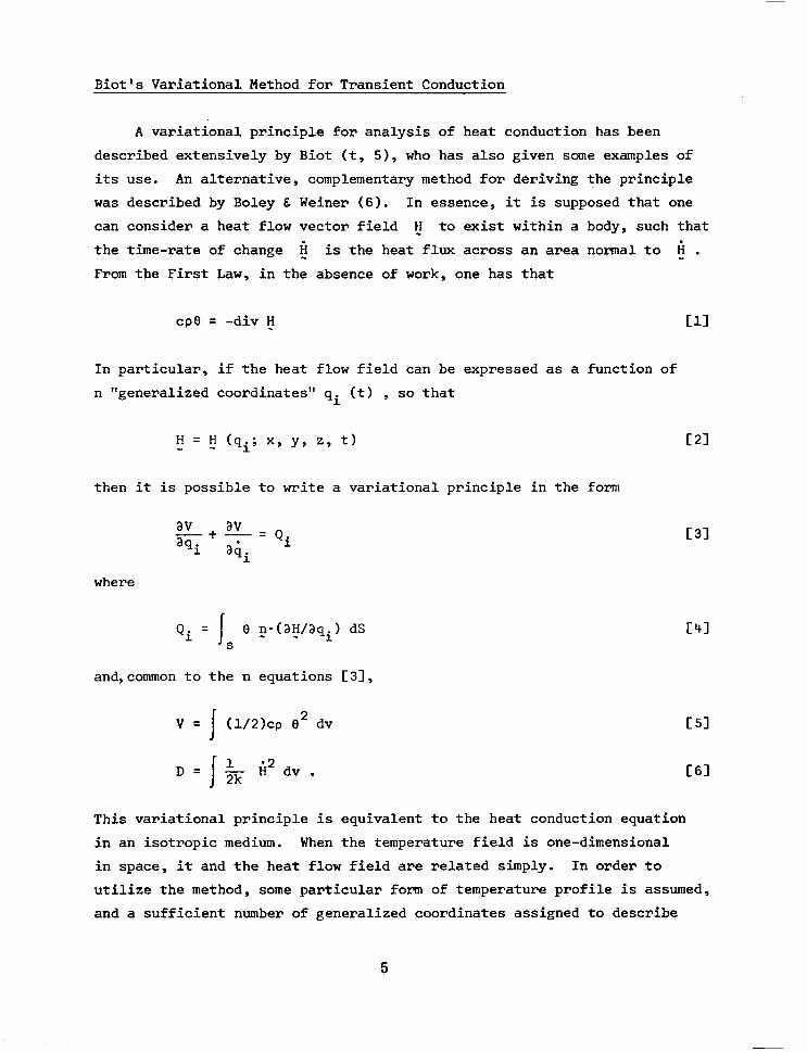
Biot's Variational Method for Transient Conduction

A variational principle for analysis of heat conduction has been

described extensively by Biot (t, 51, who has also given some examples of its use. An alternative, complementary method for deriving the principle was described by Boley & Weiner (6). In essence, it is supposed that one

can consider a heat flow vector field I;I to exist within a body, such that

the time-rate of change $ is the heat flux across an area normal to fi .

From the First Law, in the absence of work, one has that

cpe = -div F Cl1

In particular, if the heat flow field can be expressed as a function of

n "generalized coordinates" qi (t) , so that

H= H (qi; x, y¶ ', t, c21

then it is possible to write a variational principle in the form

i?!!L+i?L= aqi ai

Qi i

where

Qi = J e f?.(aG/aqi) ds S

and,common to the n equations [31,

v= J (1/2)cp e2 dv

D= & J Ii2 dv .

c33

c41

c51

C61

This variational principle is equivalent to the heat conduction equation

in an isotropic medium. When the temperature field is one-dimensional

in space, it and the heat flow field are related simply. In order to

utilize the method, some particular form of temperature profile is assumed, and a sufficient number of generalized coordinates assigned to describe

5

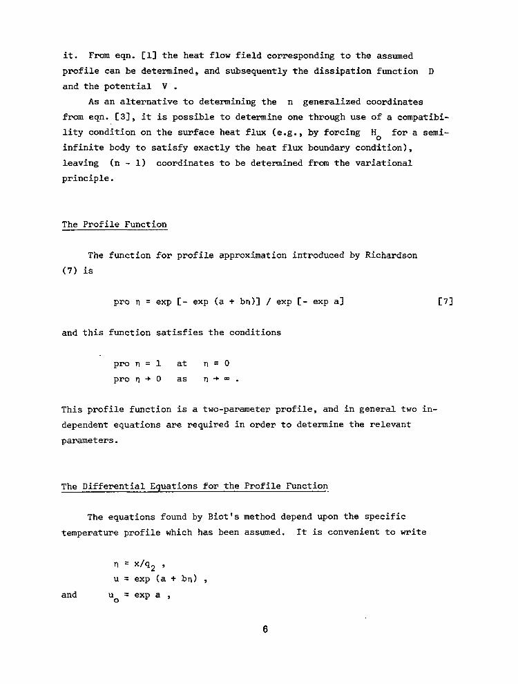
it. From eqn. Cl] the heat flow field corresponding to the assumed

profile can be determined, and subsequently the dissipation function D

and the potential V .

As an alternative to determining the n generalized coordinates

from eqn. C31, it is possible to determine one through use of a compatibi-

lity condition on the surface heat flux (e.g., by forcing Ho for-a semi-

infinite body to satisfy exactly the heat flux boundary condition),

leaving (n - 1) coordinates to be determined from the variational

principle.

The Profile Function

The function for profile approximation introduced by Richardson

(7) is

pro n = exp C- exp (a + bn)] / exp C- exp al

and this function satisfies the conditions

pro n = 1 at rl = 0

pro n + 0 as r)-+-.

This profile function is a two-parameter profile, and in general two in-

dependent equations are required in order to determine the relevant

parameters.

The Differential Equations for the Profile Function

The equations found by Biot's method depend upon the specific

temperature profile which has been assumed. It is convenient to write

c71

n = x/q2 , u = exp (a + bn) ,

and U 0

= exp a ,

6

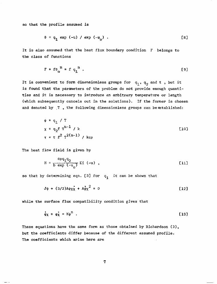
so that the profile assumed is

0 = ql exp t-u) / exp (-uo) . Cf31

It is also assumed that the heat flux boundary condition F 'belongs to

the class of functions

F = feon = f qln . c91

It is convenient to form dimensionless groups for ql, q2 and t , but it

is found that the parameters of the problem do not provide enough quanti- ties and it is necessary to introduce an arbitrary temperature or length (which subsequently cancels out in the solutions). If the former is chosen and denoted by .T , the following dimensionless groups can beestablished:

9 = ql / T

X = q2f T n-1 / k

T = t f2 T2('-l) / kcp

Cl01

The heat flow field is given by

cPqlq2 H = b exp C-u01 Ei C-u) ,

so that by determining eqn. C3l for ql it can be shown that

J$ + (3/2)AJIx); + A$K2 = 0 Cl21

Cl11

while the surface flux compatibility condition gives that

$x + qti = KJln . Cl31

These equations have the same form as those obtained by Richardson (3),

but the coefficients differ because of the different assumed profile. The coefficients which arise here are

7

A=l I O" CEi (-u)12

b2 o exp (-2uo) dn

B it =- I O" nexp t-u) Ei c-u) exp (-2~~)

dn 0

c=- Ei (-2~~)

b exp (-2~~)

D=- Ei (-uo)

b exp t-u01

Cl41

II151

Cl61

J =C-D

Cl71

K= l/D .

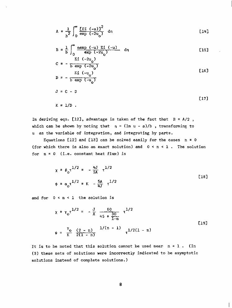
In deriving eqn. [121, advantage is taken of the fact that B = A/2 ,

which can be shown by noting that n = (In u - al/b , transforming to

U as the variable of integration, and integrating by parts.

Equations Cl21 and Cl31 can be solved easily for the cases n = 0

(for which there is also an exact solution) and 0 < n < 1 . The solution

for n = 0 (i.e. constant heat flux) is

X

and for 0 < n c 1 the solution is

l/2 = J 60 q Yof 30 T

l/2 X --

A 45 + l-n

y. (2 - n) l/(n - 1) Q= KTn=-iii

T1/2(1 - n)

Cl81

Cl91

It is to be noted that this solution cannot be used near n = 1 . (In

(3) these sets of solutions were incorrectly indicated to be asymptotic

solutions instead of complete solutions.)

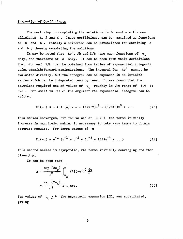
Evaluation of Coefficients

The next step in completing the solutions is to evaluate the co-

efficients A, J and K . These coefficients can be obtained as functions

of a and b . Finally a criterion can be established for obtaining a

and b , thereby completing the solutions. It may be noted that Ab3, Jb and K/b are each functions of u.

only, and therefore of a only. It can be seen from their definitions

that Jb and K/b can be obtained from tables of exponential integrals

using straightforward manipulations. The integral for Ab' cannot be

evaluated directly, but the integral can be expanded in an infinite

series which can be integrated term by term. It was found that the

solutions required use of values of u. roughly in the range of 3.0 to

8.0 . For small values of the argument the exponential integral can be

written

Ei(-u) = y t In(u) - u t (1/2!2)u2 - W3!3)u3 t . . . c201

This series converges, but for values of u > 1 the terms initially

increase in magnitude, making it necessary to take many terms to obtain

accurate results. For large values of u

Ei(-u) = ecu {u-l - uB2 t 2u -3 - (3!)u-4 t . ..I c211

This second series is asymptotic, the terms initially converging and then

diverging. It can be seen that

exp (2~~) 0~ A= J 2 du b3 u EEi(-u)) u

0

exp (2~~) =

b3 ' ' say= c221

For values of u. 1_ 4 the asymptotic expansion C21l was substituted,

giving

9

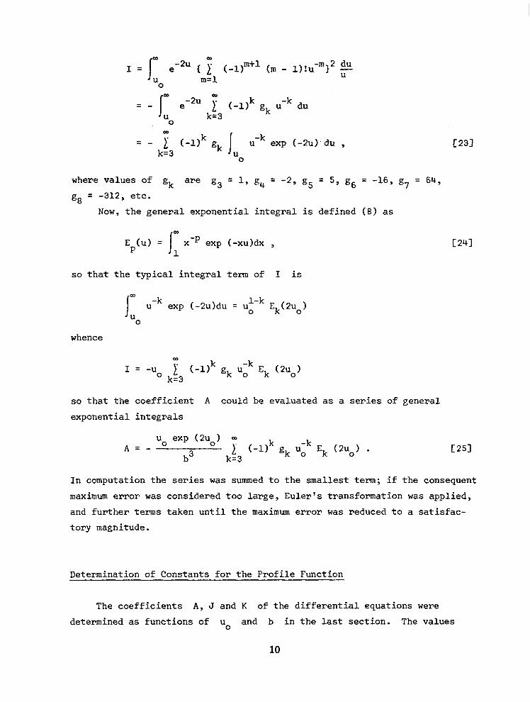
I OD

I = e-2u ( i (-l)m+l (m U m=l

- l)!u-m}2 g

0

J

OD = -

U

e-2u kT3 (-l)k gk Umk du =

Gk exp (-2~) du , II231 U

0

where values of gk are g3 = 1, g4 = -2, g5 = 5, g6 = -16, g7 = 64,

g8 = -312, etc.

Now, the general exponential integral is defined (8) as

J co

Ep(u) = x-' exp (-xu)dx , 1

so that the typical integral term of I is

J co

U-k exp (-2u)du = u. 1-k Ek(2uo) U

0

I = -u o ,", (-l)k gk uik Ek (2~~)

so that the coefficient A could be evaluated as a series of general

exponential integrals

A=- u. exp (2~~) m

2' (-l)k g b3 k=3

k uik Ek (2~~) . II251

C-1

In computation the series was summed to the smallest term; if the consequent

maximum error was considered too large, Euler's transformation was applied,

and further terms taken until the maximum error was reduced to a satisfac-

tory magnitude.

Determination of Constants for the Profile Function

The coefficients A, J and K of the differential equations were

determined as functions of u. and b in the last section. The values

10

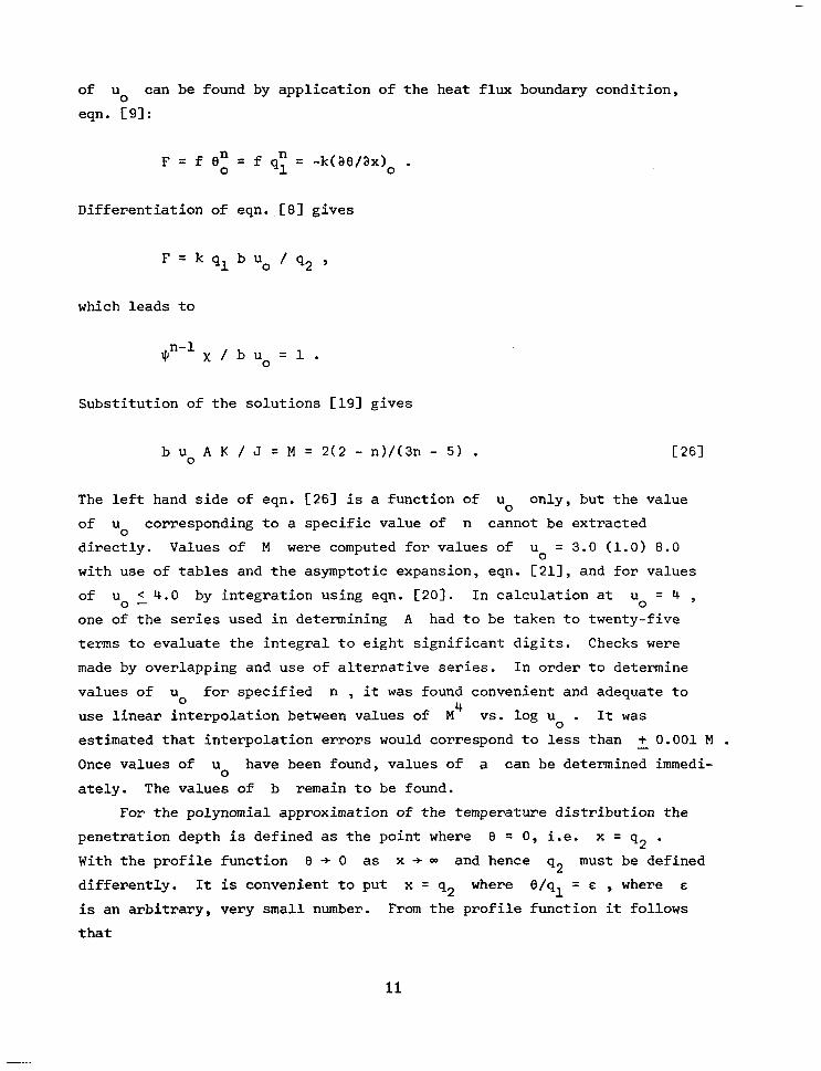
of u can be found by application of the heat flux boundary condition,

eqn. F91:

F = f 6: = f qy = -k(ae/aX)o .

Differentiation of eqn. [8] gives

F= k ql b u. 1 q2 3

which leads to

$ n-l x/bu =l. 0

Substitution of the solutions [19] gives

b u. A K / J = M = 2(2 - n)/(3n - 5) . C261

The left hand side of eqn. C261 is a function of u 0

only, but the value

of u corresponding to a specific value of n cannot be extracted 0

directly. Values of M were computed for values of u. = 3.0 (1.0) 8.0 with use of tables and the asymptotic expansion, eqn. C211, and for values

of u < 4.0 by integration using eqn. [20]. O-

In calculation at u. = 4 , one of the series used in determining A had to be taken to twenty-five terms to evaluate the integral to eight significant digits. Checks were made by overlapping and use of alternative series. In order to determine

values of u o for specified n , it was found convenient and adequate to

use linear interpolation between values of M4 vs. log u 0 - It was

estimated that interpolation errors would correspond to less than t 0.001 M , - Once values of u. have been found, values of a can be determined immedi-

ately. The values of b remain to be found. For the polynomial approximation of the temperature distribution the

penetration depth is defined as the point where 13 = 0, i.e. x = q2 .

With the profile function 8 + 0 as x + Q) and hence q2 must be defined

differently. It is convenient to put x = q2 where e/q1 = E , where E

is an arbitrary, very small number. From the profile function it follows

that

11

b= ln(1 - eBa In E) . [271

It was decided to use e = 0.01 here. It must be emphasized that the value of b depends upon the value of E . With this convention, it is not

significant to compare directly the coefficients of the penetration depth solutions from use of polynomial and transcendental profiles.

Results and Accuracy of Computations

C281

Constant-flux solution The values found for the constant-flux

solution were u 0

= 2.95 ,

JI q 1.130 P2

X = 3.18 ~~~~

which can be compared with Richardson's (3) parabolic approximation

JI = 1.157 t1'2 ; x = 2.59 P2

and with the exact solution

J, = 1.1284 ~~~~ .

It can be seen that the coefficient for $1~ l/2 using the profile function differs from the exact solution by about 0.2 per cent and from the para-

bolic approximation by about 2.4 per cent.

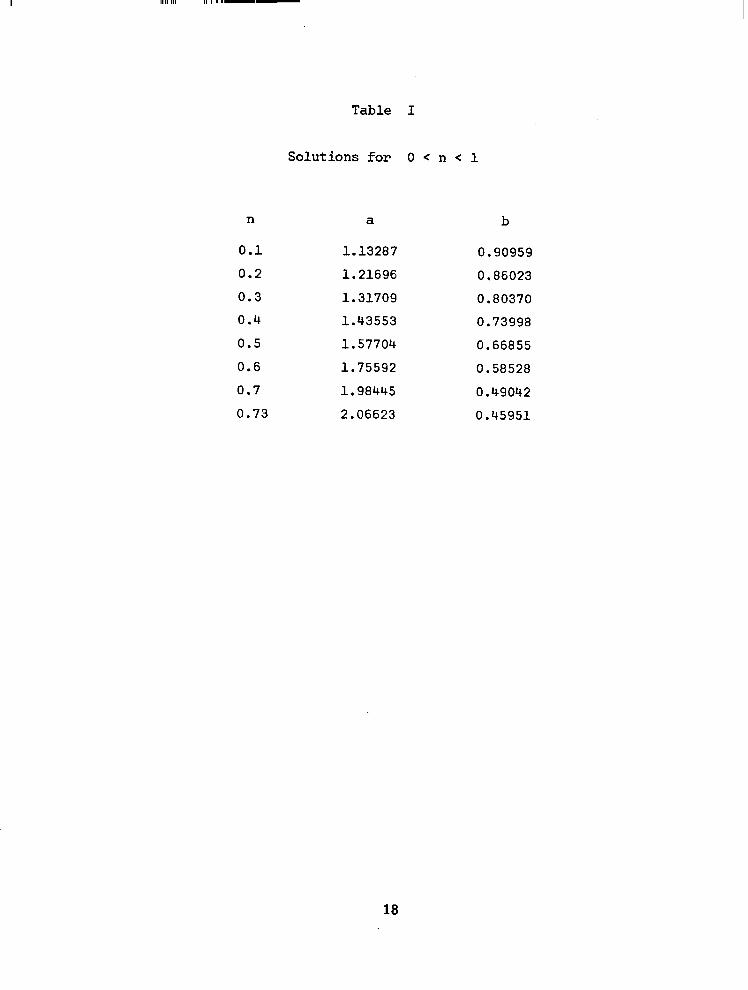
Solutions for n > 0 A set of solutions was computed for a range of

n where the computations did not become inordinately long. In Table I

values of a and b are provided, and in Table II values of the surface

temperature coefficients JI/T 1/2(1-n) (p arabolic profile), $/T 1/2(1-n)

(transcendental profile) and penetration depth coefficient (transcendental

profile) are listed, together with the percentage differences of the sur-

face temperature coefficients.

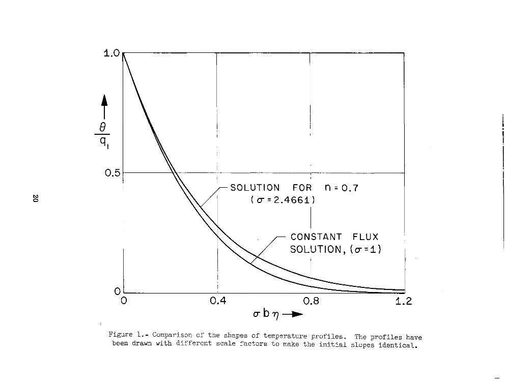
For the sake of comparison, two temperature profiles have been plotted

12

in Fig. 1. The scale of slab depth n has been ,adjusted by using scaling factors u so that both profiles have the same slope at rj=o. It can be seen that the profile for the constant-flux solution has a somewhat different shape from that for the solution with n q 0.7 . Profiles for intermediate values of n fall between those shown.

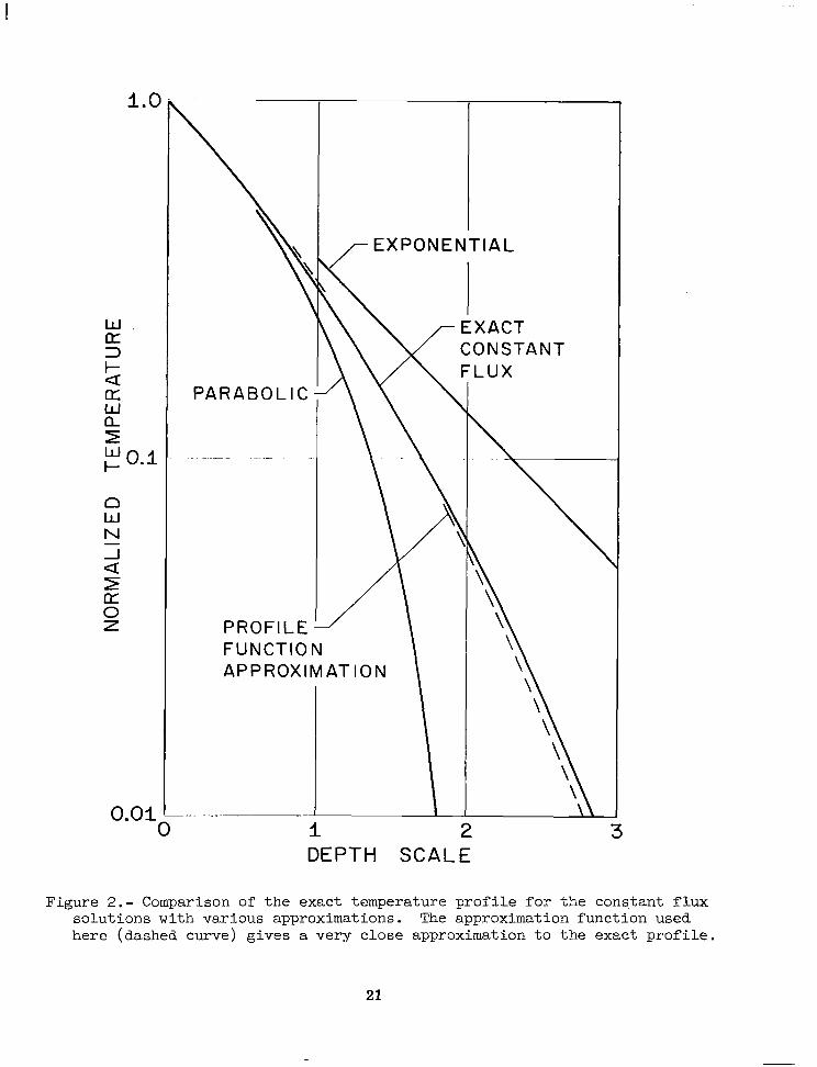
Another comparison has been made in Fig. 2 for the constant-flux solution. The ordinate is of temperature, normalized such that the temperature on the axis (which corresponds to the body surface) is always unity; the abscissa, the slab depth, has been adjusted such that all temperature profiles shown have a slope of unity at the body surface. The middle solid line represents the profile of the analytic solution of the

constant flux case; two other solid lines represent the parabolic and the simple exponential approximations respectively. The dashed line represents the profile approximation used here. Since this lies so close to (and crosses) the analytic solution, only parts can be shown without obscuring the analytic solution. This figure demonstrates well that the profile function used here is a closer approximation than are the others cited.

The computations using the exponential integrals were based upon the tables of Pagurova (8), with values for integrals beyond the range of the tables generated using relations given in the same reference. Computations for other quantities described here were made using the handbook of Abramowich and Stegun (9), with checks being made in relevant references given therein. The accuracy of the computations varies with n in the solutions, but it is believed to be not worse than 0.1 per cent in any

case.

Analytic Solutions for n = 1.0

The analytic solution for n = 0 , i.e. constant heat flux, is well

known. The problem can also have an analytic solution at n = 1.0 if the initial condition described in the Introduction is slightly altered so that the slab temperature is uniform but above the reference zero by an arbitrary amount. Without this alteration the solution recovered is the trivial case 3(x, t) = 0 . The arbitrary uniform temperature can be

chosen as the unit temperature of the 8 temperature scale; the solution

13

is proportional to it. The solution can be written

cl(x, t) - 1 = E Mm+l t(m+1)/2 irnl$::f:;i")

m=O 1 c291

with

M m+l = r( F+ 1) Mm

tf2 xf T=)CCP' 5 =-

2k

(where f has been normalized with respect to the initial temperature).

The function im erfcn is the m-th repeated integral of the error function,

for which useful tables, recurrence relations, expansions and so forth

exist. At small times, the term for m = 0 is dominant and this coincides

with the constant flux solution discussed previously, For longer times, the series provides a shifting average of the repeated integrals of the error

function. Successive integrals have profile shapes which move from the

central profile of Fig. 2 towards the simple exponential. The approximate

profiles found here for 0 < n < 1.0 have a trend in the same direction.

For very long times, the asymptotic behavior of im erfcn as m-t= is

important. This can be determined from the series expansion

1 'm erfcn = T (-1>p ,p p=o 2"-P p! r(1 + Y)

in which the terms corresponding to p = mt2, mt4, mt6, .., are under-

stood to be zero. As m tends to infinity, it can be shown that the

normalized repeated integral of the error function (i" erfcn/im erfc0)

is given asymptotically by a simple negative exponential function of n .

Discussion

It can be seen from Fig. 1 that the solution of the problem does

take advantage, so to speak, of the flexibility of the transcendental

14

profile by finding that different shapes are appropriate to different

conditions. This adaptive feature of the transcendental profile should assist in providing results which are more accurate than with fixed simple profiles. This hope is borne out clearly in the constant-flux solution, where the accuracy of the surface temperature coefficient is

improved by a tenfold order of magnitude compared with the simple poly- nomial and exponential profiles listed in Table I of Lardner's paper (2).

It is also demonstrated by Fig. 2. For 0 < n c 1.0 no exact solutions exist with which the results

can be compared. The calculations become increasingly difficult as n

approaches unity. This is due partly to the need to generate exponential integrals beyond the range of available tables, and partly to the behavior of the profile function. In the profile function the parameter a essen-

tially specifies the shape of the profile, while the parameter b specifies the extent of the profile. Thus, two profiles drawn with the same values of a and different values of b have the same shape, but

not vice versa. As a + 0~ , pron + exp [-(b exp a)n 1. Over the major range of pro0 , this limit is approached rapidly. Even with a = 5.0 , pron is close to its limit. This means that if an attempt is made to fit the profile function to a function which is close to the simple exponential, the determination of a becomes extremely insensitive; large changes in a

produce small changes in the profile shape. It is increasingly difficult to obtain values of a to a specified number of significant digits.

It is noteworthy that the difference between the surface temperature coefficients listed in Table II increases smoothly from the value of 2.4%

at n = 0 to 12% at n = 0.73 , the difference increasing roughly expo-

nentially with n . The difference between surface temperature coefficients

is sufficiently large to be significant in application. These differences occur because the transcendental profile changes

its shape with n , which the parabolic profile cannot do. It is very

probable that the solutions with the transcendental profile are more accurate, but at present this cannot be demonstrated directly. However,

it is possible to make comparisons with the analytical solutions for n= 0

and n= 1.0 and show that the temperature profile shape generated here

for 0 < n < 1.0 varies smoothly between the analytic limits. The signi- ficant feature of the results upon which a comparison can be based is the

15

parameter a , which determines the shape of the profile. It has been noted above that the asymptotic behavior of the analytic solution for

n = 1.0 is that the profile becomes a simple exponential; in approximat-

ing this shape a becomes large. For n = 0 , the short-time solution is valid at all times, so that in this instance it is also the long-time

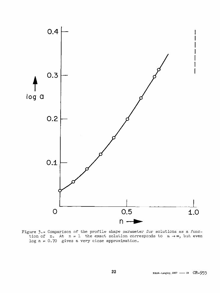
solution. The values of a for solutions in the range 0 < n < i.0 are

shown in Fig. 3. In this it can be seen that the values found here fit

well between the analytic limits. This feature is absent in all fixed

profiles, such as polynomials. The comparison provides conducive evidence

that the solutions presented here are considerably more accurate than the

corresponding solutions available previously.

Summary

(1)

(2)

(3)

(4)

(5)

Biot's variational method is applied to a problem of transient

heat conduction in a semi-infinite slab subject to a non-linear

boundary condition.

A two-parameter transcendental approximation is used for the

temperature profile. This approximation has the advantage that its

shape is not fixed, so that the profile determined for each case

considered can have the shape most appropriate to it.

Computations for solutions utilizing the general exponential

integral are described, and two exact solutions are mentioned for

cases which bound the examples computed.

Comparison of the variational solution using the transcendental

approximation with the exact solution for the limiting case of

constant heat flux demonstrates an error of less than 0.2 per cent

in the surface temperature coefficient and very close representation

of the true temperature profile. This corresponds to a very consider-

able improvement over solutions obtained previously with other

profile approximations. Comparison of the variational solution for other examples shows

that the computed profile shapes have a uniform variation which is

in the correct direction to merge with the limiting case of surface

heat flux directly proportional to surface temperature.

16

(6) It is concluded that the solutions obtained here using the transcendental approximation are considerably more accurate than those previously available.

Acknowledeements

The authors are grateful to Mr. S. H. Kozak, Research Assistant, Division of Engineering, Brown University, who made a complete check of the computations and extended the range of the-long-time solutions. The

-work was supported by the U. S. National Aeronautics and Space Admini- stration under Grant NGR-40-002-012, .and this support is gratefully acknowledged.

REFERENCES

(1)

(2)

(3)

(4)

(5)

(6)

(7)

(8)

(9)

Hanson, F. B. and Richardson, P. D. "Use of a transcendental approxi- mation in laminar boundary layer analysis" Jl. Mech. Engng. Sci. vol. 7, p. 131, 1965.

Lardner, T. J. "Biot's variational principle in heat conduction" A.I.A.A. Jl. vol. 1, p. 196, 1963.

Richardson, P. D. "Unsteady one-dimensional heat conduction with a non-linear boundary condition" A.S.M.E. Jl. of Heat Transfer vol. 86, p. 298, 1964.

Biot, M. A. "Linear thermodynamics and the mechanics of solids" Proc. 3rd U. S. National Congress of Applied Mech., A.S.M.E., p. 1, 1958.

Biot, M. A. "New methods in heat flow analysis with application to flight structures" Jl. Aero. Sci., vol. 24, p. 857, 1957.

Boley, B. A. and Weiner, J. H. Theory of thermal stresses, J. Wiley and Sons, New York, 1960.

Richardson, P. D. "Transcendental approximation for laminar boundary layers lr A.I.A.A. Jl., vol. 1, p. 2659, 1963.

Pagurova, V. I. Tables of the exponential integral, translated by D. L. Fry, Pergamon Press, New York, 1961.

Abramowich, M. and Stegun, I. A. teds.) Handbook of mathematical functions, U. S. Govt. Printing Office, Washington, D. C., 1964.

17

n a b

0.1 1.13287 0.90959 0.2 1.21696 0.86023 0.3 1.31709 0.80370 0.4 1.43553 0.73998 0.5 1.57704 0.66855

0.6 1.75592 0.58528 0.7 1.98445 0.49042

0.73 2.06623 0.45951

Table I

Solutions for 0 c n < 1

18

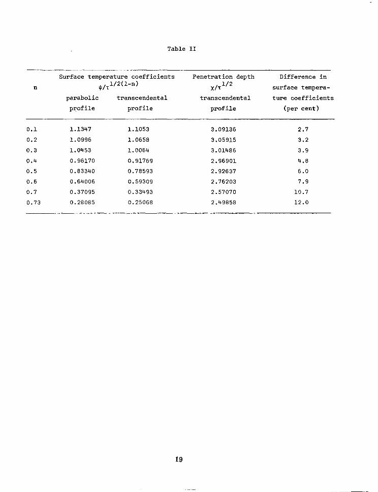
Table II

Surface temperature coefficients Penetration depth Difference in

n O/T 1/2(1-n)

X/T l/2 surface tempera-

parabolic transcendental transcendental ture coefficients

profile profile profile (per cent)

0.1 1.1347 1.1053 3.09136 2.7

0.2 1.0996 1.0658 3.05915 3.2

0.3 1.0453 1.0064 3.01486 3.9

0.4 0.96170 0.91769 2.96901 4.8

0.5 0.83340 0.78593 2.92637 6.0

0.6 0.64006 0.59309 2.76203 7.9

0.7 0.37095 0.33493 2.57070 10.7

0.73 0.28085 0.25068 2.49858 12.0

19

1.0

t 8

ql

0.5 SOLUTION FOR n q 0.7

( u- = 2.4661)

CONSTANT FLUX SOLUTION, (cr=l)

0.4 0.8 1.2

! .

Figure l.- Comparison of the shapes of temperature profiles. The profiles have been dram with different scale factors to make the initial slopes identical.

\

\

\ \

PA RABOLI C

PROFIL E

,-EXPONENTIAL

FUNCTION APPROXIMATION

ACT NSTANT ux

\ \ \ 1 \ \ \

1 2 3 DEPTH SCALE

Figure 2.- Comparison of the exact temperature profile for the cons,tant flux solutions with various approximations. The approximation function used here (dashed curve) gives a very close approximation to the exact profile.

21

f

log a

0.4

0.3

0.2

0.1

0 I

0.5 -~ L

1.0 n+

Figure 3.- Comparison of the profile shape parameter for solutions as a func- tion of n. At n = 1 the exact solution corresponds to a +a~, but even log a = 0.70 gives a very close approximation.

22 NASA-Langley, 1967 - 19 CR-955

“The aeronautical and space activities of the United States shall be conducted so as to contribute . . . to the expansion of hman knowl- edge of phenomena in the atmosphere and space. The Administration shall provide for the widest practicable and appropriate dissemination of information concerning its activities and the resrdts thereof.”

-NATIONAL AERoruuncs AND SPACE Acr OF 19.58

NASA SCIENTIFIC AND TECHNICAL PUBLICATIONS

TECHNICAL REPORTS: Scientific and technical information considered important, complete, and a lasting contribution to existing knowledge.

TECHNICAL NOTES: Information less broad in scope but nevertheless of importance as a contribution to existing knowledge.

TECHNICAL MEMORANDUMS: Information receiving limited distribu- tion because of preliminary data, security classification, or other reasons.

CONTRACTOR REPORTS: Scientific and technical information generated under a NASA contract or grant and considered an important contribution to existing knowledge.

TECHNICAL TRANSLATIONS: Information published in a foreign language considered to merit NASA distribution in English.

SPECIAL PUBLICATIONS: Information derived from or of value to NASA activities. Publications include conference proceedings, monographs, data compilations, handbooks, sourcebooks, and special bibliographies.

TECHNOLOGY UTILIZATION PUBLICATIONS: Information on tech- nology used by NASA that may be of particular interest in commercial and other non-aerospace applications. Publications include Tech Briefs, Technology Utilization Reports and Notes, and Technology Surveys.

Details on the availabihy OF these publications may be obtained from:

SCIENTIFIC AND TECHNICAL INFORMATION DIVISION

NATIONAL AERONAUTICS AND SPACE ADMINISTRATION

Washington, D.C. 20545