Embed Size (px)
Citation preview

11
Usage of Process Capability Indices During Development Cycle of Mobile Radio Product
Marko E. Leinonen Nokia Oyj
Finland
1. Introduction
Mobile communication devices have become a basic need for people today. Mobile devices are used by all people regardless of the race, age or nationality of the person. For this reason, the total number of mobile communication devices sold was almost 1.6 billion units worldwide during 2010 (Gartner Inc., 2011). Manufacturability and the level of quality of devices need to be taken into account at the early stages of design in order to enable a high volume of production with a high yield.
It is a common and cross-functional task for each area of technology to build the required level of quality into the end product. For effective communication between parties, a common quality language is needed and process capability indices are widely used for this purpose.
The basis for the quality is designed into the device during the system specification phase
and it is mainly implemented during the product implementation phase. The quality level is
designed in by specifying design parameters, target levels for the parameters and the
appropriate specification limits for each parameter. The quality level of the end product
during the manufacturing phase needs to be estimated with a limited number of
measurement results from prototype devices during the product development phase.
Statistical methods are used for this estimation purpose. A prototype production may be
considered to be a short-term production compared to the life cycle of the end product and a
long-term performance process is estimated based on the short-term production data. Even
though statistical process control (SPC) methods are widely used in high volume
production, the production process may vary within statistical control limits without being
out of the control leading product to product variation between product parameters.
Easy to use statistical process models are needed to model long-term process performance
during the research and development (R&D) phase of the device. Higher quality levels for
the end product may be expected, if the long-term variation of the manufacturing process is
taken into account more easily during the specification phase of the product’s parameters.
2. Product development process
An overview of a product development process is shown in Figure 1 (based on Leinonen, 2002). The required characteristics of a device may be defined based on a market and
www.intechopen.com

Systems Engineering – Practice and Theory
234
competitor analyses. A product definition phase is a cross-functional task where marketing and the quality department and technology areas together define and specify the main functions and target quality levels for features of the device. A product design phase includes system engineering and the actual product development of the device. The main parameters for each area of technology as well as the specification limits for them are defined during the system engineering phase. The specification limits may be ‘hard’ limits which cannot be changed from design to design, for example governmental rulings (e.g., Federal Communications Commission, FCC) or standardisation requirements (e.g., 3GPP specifications) or ‘soft’ limits, which may be defined by the system engineering team.
Customer & Market NeedsMarket segmentation
Product DefinitionMulti-discipline work
Product DesignSystem designDesign implementation
Design testingPrototype testingReliability testing
Design reviews:- Check for all processes & stds.- Product definition- Design standards- Testing Analysis- Quality Requirements
Manufacturing Process- Quality assurance e.g.Statistical process control
Selling & Delivery
Competition AnalysisMinimum Product Requirements Design Standards
- Standardization requirements(electronic, mechanical…)- Standard product requirements- Product reliability / quality requirements- Approved/Certified parts- Experience from previous designs- Design of Experiment- Failure mode & Effect Analysis- Design for Manufacturability
Fig. 1. An overview of a product development process
The main decisions for the quality level of the end product are done during the system engineering and product design phases. Product testing is a supporting function which ensures that the selections and implementations have been done correctly during the implementation phase of the development process. The quality level of the end product needs to be estimated based on the test results prior to the design review phase, where the maturity and the quality of the product is reviewed prior the mass production phase. New design and prototype rounds are needed until the estimated quality level reaches the required level. Statistical measures are tracked and stored during the manufacturing phase of the product and those measures are used as a feedback and as an input for the next product development.
2.1 Process capability indices during the product development
An origin of process capability indices is in the manufacturing industry where the performance of manufacturing has been observed with time series plots and statistical process control charts since 1930s. The control charts are useful for controlling and monitoring production, but for the management level a raw control data is too detailed and thus a simpler metric is needed. Process capability indices were developed for this purpose and the first metric was introduced in early 1970s. Since then, numerous process capability indices are presented for univariate (more than twenty) and multivariate (about ten) purposes (Kotz & Johnson, 2002). The most commonly used process capability indices are
www.intechopen.com

Usage of Process Capability Indices During Development Cycle of Mobile Radio Product
235
still Cp and Cpk which are widely used within the automotive - an electrical component - the telecommunication and mobile device industries. An overview of the use of process capability indices for quality improvement during the manufacturing process (based on Albing, 2008; Breyfogle 1999) is presented in Figure 2.
Identify a important parameterPlan the study
Establish statistical control,Gather data
Initiate the improvement actions
Assess the capability of the process
Fig. 2. An improvement process for production related parameters
The usage of process capability indices has been extended from the manufacturing industry to the product development phase, where the improvement of the quality level during product development needs to be monitored, and process capability indices are used for this purpose. The main product development phases, where product capability indices are used, are shown in Figure 3.
Collect data from a mass production
A new project definitionA data from a pilot production
Implementation of DesignTesting of prototype devices
System design phase e.g.Tolerance analysis
Fig. 3. Product development steps where process capability indices are actively used
An advantage of process capability indices is that they are unitless, which provides the possibility of comparing the quality levels of different technology areas to each other during the development phase of the mobile device, for the example mechanical properties of the device may be compared to radio performance parameters. Additionally, process capability indices are used as a metric for quality level improvement during the development process of the device. The following are examples of how process capability indices may be used during the product development phase:
A common quality level tool between R&D teams during the product definition phase and business-to-business discussions
An estimate for the expected quality level of the end product during the R&D phase
www.intechopen.com
Systems Engineering – Practice and Theory
236
A robustness indicator of design during the R&D phase and product testing
A decision-making tool of the quality level during design reviews
A process capability indicator during the mass production phase
A tool to follow the production quality for quality assurance purposes
Process capability indices can be calculated with some statistical properties of data regardless of the shape of a data distribution. The shape of the data needs to be taken into account if the product capability index is mapped to an expected quality level of the end product. Typically, normal distributed data is assumed for simplicity, but in real life applications a normality assumption is rarely available, at least in radio engineering applications. One possibility to overcome the non-normality of the data is to transform the data closer to the normal distribution and to calculate the process capability indices for the normalised data (Breyfogle, 1999); however, this normalisation is not effective for all datasets. An alternative method is to calculate the process capability indices based on the probability outside of the specification limits and to calculate the process capability index backwards.
2.2 RF system engineering during the product development
RF (Radio Frequency) engineering develops circuitries which are used for wireless
communication purposes. RF system engineering is responsible for selecting the appropriate
RF architectures and defining the functional blocks for RF implementations. System
engineering is responsible for deriving the block level requirements of each RF block based
on specific wireless system requirements, e.g., GSM or WCDMA standards and regulatory
requirements such as FCC requirements for unwanted radio frequency transmissions.
RF system level studies include RF performance analyses with typical component values as
well as statistical analyses with minimum and maximum values of components. The
statistical analyses may be done with statistical software packages or with RF simulators in
order to optimise performance and select the optimal typical values of components for a
maximal quality level. RF block level analyses with process capability indices are studied in
Leinonen (1996) and a design optimisation with process capability contour plots and process
capability indices in Wizmuller (1998). Most of the studied RF parameters are one-
dimensional parameters which are studied and optimised simultaneously, such as the
sensitivity of a receiver, the linearity of a receiver and the noise figure of a receiver.
Some product parameters are multidimensional or cross-functional and need a multidimensional approach. A multiradio operation is an example of a multidimensional radio parameter, which requires multidimensional optimisation and cross-technology communication. The requirements for the multiradio operation and interoperability need to be agreed as a cross-functional work covering stake holders from product marketing, system engineering, radio engineering, testing engineering and the quality department. The requirement for multiradio interoperability - from the radio engineering point of view - is a probability when the transmission of the first radio interferes with the reception of a second radio. The probability may be considered as a quality level, which may be communicated with a process capability index value and which may be monitored during the development process of the device. A multiradio interoperability (IOP) may be presented with a two-dimensional figure, which is shown in Figure 4 (based on Leinonen, 2010a). Interference is present if the signal condition is within an IOP problem area. The probability of when this
www.intechopen.com

Usage of Process Capability Indices During Development Cycle of Mobile Radio Product
237
situation may occur can be calculated with a two dimensional integral, which includes the probabilities of radio signals and a threshold value. The actual threshold value for the transmission signal level is dependent on - for example - an interference generation mechanism, an interference tolerance of the victim radio and the activity periods of radios.
f(x)
Minimum transmission level
Minimumreception level
Maximumreception level
Maximumtransmission level
Multiradiointeroperability OKf(y)
IOPProblem
Fig. 4. Illustration of multiradio interoperability from the RF system engineering point of view
3. Overview of process capability indices
Process capability indices are widely used across different fields of industry as a metric of the quality level of products (Breyfogle, 1999). In general, process capability indices describe a location of a mean value of a parameter within specification limits. The specification limits can be ‘hard’ limits, which cannot be changed from product to product, or ‘soft’ limits, which are defined during the system engineering phase based on the mass production data of previous or available components, or else the limits are defined based on numerical calculations or simulations.
The most commonly used process capability indices within industry are so-called ‘first generation’ process capability indices Cp and Cpk. The Cp index is (Kotz S. & Johnson, 1993)
6
p
USL LSLC
, (1)
where USL is an upper specification limit and LSL is a lower specification limit, and σ is a
standard deviation unit of a studied parameter. Cpk also takes the location of the parameter
into account and it is defined (Kotz S. & Johnson, 1993)
min ,3 3
pk
USL LSLC
, (2)
where μ is a mean value of the parameter. The process capability index Cpk value may be
converted to an expected yield with a one-sided specification limit (Kotz S. & Johnson, 1993)
Yield 3 pk C
, (3)
www.intechopen.com

Systems Engineering – Practice and Theory
238
where Φ is a cumulative probability function of a standardised normal distribution. A probability outside of the specification limit is one minus the yield, which is considered to be a quality level. A classification of process capability indices and expected quality levels are summarised in Table 1 (Pearn and Chen, 1999; Leinonen, 2002). The target level for Cpk in high volume production is higher than 1.5, which corresponds to a quality level of 3.4 dpm (defects per million)
Acceptable level Cpk value Low limit High limit Poor 0.00 Cpk < 0.50 500000 dpm 66800 dpm
Inadequate 0.50 Cpk < 1.00 66800 dpm 1350 dpm
Capable 1.00 Cpk < 1.33 1350 dpm 32 dpm
Satisfactory 1.33 Cpk < 1.50 32 dpm 3.4 dpm
Excellent 1.50 Cpk < 2.00 3.4 dpm 9.9*10-4 dpm
Super Cpk 2.00 9.9*10-4 dpm
Table 1. A classification of the process capability index values and expected quality level
The Cpk definition in equation 2 is based on the mean value and the variation of the data, but alternatively the Cpk may be defined as an expected quality level (Kotz S. & Johnson, 1993)
-1pk
1
3C , (4)
where γ is the expected proportion of non-conformance units.
Data following a normal distribution is rarely available in real life applications. In many cases, the data distribution is skewed due to a physical phenomenon of the analysed parameter. The process capability analysis and the expected quality level will match each other if the shape of the probability density function of the parameter is known and a statistical analysis is done based on the distribution. The process capability index Cpk has been defined for non-normally distributed data with a percentile approach, which has now been standardised by the ISO (International Standardisation Organisation) as their definition of the Cpk index. The definition of Cpk with percentiles is (Clements, 1989)
USL-M M-LSLmin ,
M Mp p
pkCU L
, (5)
where M is a median value, Up is a 99.865 percentile and Lp is a 0.135 percentile.
A decision tree for selecting an approach to the process capability analysis is proposed in Figure 5. The decision tree is based on the experience of the application of process capability indices to various real life implementations. The first selection is whether the analysed data is a one-dimensional or a multidimensional. Most of the studied engineering applications have been one-dimensional, but the data is rarely normally distributed. A transform function, such as a Cox-Box or a Johnson transformation, may be applied to the data to convert the data so as to resemble a normal distribution. If the data is normally distributed, then the results based on equations 2 and 3 will match each other. If a probability density function of the parameter is known, then the process capability analysis should be done with the known distribution. Applications for this approach are discussed in Chapter 4. The process capability analysis based on equation 5 is preferred for most real-life applications.
www.intechopen.com

Usage of Process Capability Indices During Development Cycle of Mobile Radio Product
239
In general, the analysis of multidimensional data is more difficult than one-dimensional data. A correlation of the data will have an effect to the analysis in the multidimensional case. The correlation of the data will change the shape and the direction of the data distribution so that the expected quality level and calculated process capability index do not match one another. A definition of a specification region for multidimensional data is typically a multidimensional cube, but it may alternatively also be a multidimensional sphere, which is analysed in Leinonen (2010b). The process capability analysis may be done with analytical calculus or numerical integration of multidimensional data, if the multidimensional data is normally distributed (which is rarely the case). Transformation functions are not used for non-normally distributed multidimensional data. A numerical integration approach for process capability analysis may be possible for non-distributed multidimensional data but it may be difficult with real life data. A Monte Carlo simulation-based approach has been preferred for non-normally distributed multidimensional data. The process capability analysis has been done based on equation 3, where simulated probability out of the specification region is converted to a corresponding Cpk value. The Monte Carlo simulations are done with computers, either with mathematical or spread sheet software based on the properties of the statistical distribution of the data.
Process performance indices Pp and Ppk are defined in a manner similar to the process
capability indices Cp and Cpk, but the definition of the variation is different. Pp and Ppk are
defined with a long-term variation while Cp and Cpk are defined with a short-term variation (Harry & Schroeder, 2000). Both the short-term and the long-term variations can be
distinguished from each other by using statistical control charts with a rational sub-grouping of the data in a time domain. The short-term variation is a variation within a sub-group and
the long-term variation sums up short-term variations of sub-groups and a variation between sub-group mean values, which may happen over time. Many organisations do distinguish
between Cpk and Ppk due to similar definitions of the indices (Breyfogle, 1999).
Process/Design Capability analysis for continuous data
One-dimensional data
Normal distributed
- Normal distribution Cpk analysis
Data Normalization
Non-normal distributed
- Cpk analysis with aknown distribution- Clements's method
Normal distributed Non-Normally distributed
Uncorrelated data
Multi-dimensional data
- Multidimensional Cpk analysis- Numerical or Simulation based analysis- out of spec. based Cpk
Correlated data
Normal distributed
- Numerical or Simulation based analysis- out of spec. based Cpk
Fig. 5. Process capability analysis selection tree
3.1 Statistical process models for manufacturability analysis
An overview of the usage of process capability analyses during the product development process is shown in Figure 6. Data from a pilot production is analysed in R&D for development purposes. These process capability indices provide information about the
www.intechopen.com

Systems Engineering – Practice and Theory
240
maturity level of the design and the potential quality level of the design. The pilot production data may be considered as a short-term variation of the device as compared with a mass production (Uusitalo, 2000). Statistical process models for sub-group changes during a mass production process are needed in order to estimate long-term process performance based on the pilot production data. A basic assumption is that the manufacturing process is under statistical process control, which is mandatory for high volume device production. A mean value and a variation of the parameters are studied during mass production. The mean values of parameters change over time, since even if the process is under statistical process control, statistical process control charts allow the process to fluctuate between the control limits of the charts.
Process performance index estimation
Actual Process performance index
Statistical long-term process modelling
Process capabilityindex estimation
A pilot production and production data
A mass productionand production data
Research and development
Manufacturing
A design of device
Fig. 6. Long-term process performance estimation during product development
An ideal process is presented in Figure 7, where the mean value and the variation of the process are static without a fluctuation over time. There are some fluctuations in real life processes and those are controlled by means of statistical process control. SPC methods are based on a periodic sampling of the process, and the samples are called sub-groups. The frequency of sampling and the number of samples within the sub-group are process-dependent parameters. The size of the sub-group is considered to be five in this study, which has been used in industrial applications and in a Six Sigma process definition. The size of sub-group defines control limits for the mean value and the standard deviation of the process. The mean value of sub-groups may change within +/- 1.5 standard deviation units around the target value without the process being out of control with a sub-group size of five. The variation of the process may change up to an upper process control limit (B4) which is 2.089 with a sub-group size of five.
The second process model presented in Figure 8 is called a Six Sigma community process model. If the mean value of the process shifts from a target value, the mean will shift 1.5 standard deviation units towards the closer specification limit and the mean value will stay there. The variation of the process is a constant over time in the Six Sigma process model, but it is varied with a normal and a uniform distribution in Chapter 3.2.
The mean value of the process varies over time within control limits, but the variation is a
constant in the third process model presented in Figure 9. The variation of the mean value
within the control limits is modelled with a normal and a uniform distribution.
The mean value and the variation of the process are varied in the fourth process model presented in Figure 10. The changes of the mean value and the variation of sub-groups may
www.intechopen.com

Usage of Process Capability Indices During Development Cycle of Mobile Radio Product
241
be modelled with both a normal and a uniform distribution. The normal distribution is the most common distribution for modelling a random variation. For example, tool wear in the mechanical industry produces a uniform mean value shift of the process over time.
A short-term process deviation is calculated from the ranges of sub-group and a long-term variation is calculated with a pooled standard deviation method over all sub-groups (Montgomery, 1991). If the number of samples of the sub-group is small - i.e., less than 10 - the range method in deviation estimation is preferred due to the robustness of outlier observations (Bissell, 1990). For control chart creation, 20 to 25 sub-groups are recommended (Lu & Rudy, 2002). It is easier and safer to use a pooled standard deviation method for all the data in an R&D environment for the standard deviation estimation to overcome time and order aspects of the data.
...
Grand average
-1.5 short-term deviation units
-3.0 short-term deviation units
Sub-group 1 Sub-group N
Total dataPopulation
+3.0 short-term deviation units
+1.5 short-term deviation units
Long-term parameterdeviation
Time
Parameter value
Fig. 7. An ideal process model without mean or deviation changes
...
Grand average
-1.5 short-term deviation units
-3.0 short-term deviation units
Sub-group 1 Sub-group N
Total dataPopulation
+3.0 short-term deviation units
+1.5 short-term deviation units
Long-term parameterdeviation
Time
Parameter value
Fig. 8. A Six Sigma process model with a constant mean value shift of sub-groups
...
Grand average
-1.5 short-term deviation units
-3.0 short-term deviation units
Sub-group 1 Sub-group NTotal dataPopulation
+3.0 short-term deviation units
+1.5 short-term deviation units
Long-term parameterdeviation
Time
Parameter value
Fig. 9. A process model with a variable mean value and a constant variation of sub-groups
www.intechopen.com

Systems Engineering – Practice and Theory
242
...
Grand average
-1.5 short-term deviation units
-3.0 short-term deviation units
Sub-group 1 Sub-group N
Total dataPopulation
+3.0 short-term deviation units
+1.5 short-term deviation units
Long-term parameterdeviation
Time
Parameter value
Fig. 10. A process model with a variable mean value shift and variations of sub-groups
3.2 Process model effect to one-dimensional process performance index
Long-term process performance may be estimated based on short-term process capability
with a statistical process model. The easiest model is a constant shift model, which is
presented in Figure 8. The mean value of sub-groups is shifted with 1.5 deviation units with
a constant variation. The process performance index is (Breyfogle, 1999)
min 0.5, 0.53 3
pk
USL LSL P , (6)
where σ is a short-term standard deviation unit.
A constant variation within sub-groups with a varied mean value of sub-groups is presented
in Figure 9. It is assumed that the variation of the mean value of sub-groups is a random
process. If the variation is modelled with a uniform distribution within statistical control limits
(+/- 1.5 standard deviation units), then long-term process standard deviation is
2
2 2Long term
1.5 1.5 71.330
12 2 (7)
and a corresponding long-term process performance index Ppk is
min , min ,3 1.330 3 1.330 3.99 3.99
pk
USL LSL USL LSL
P . (8)
The second process model for the variation of the mean values of the sub-groups of the
process presented in Figure 9 is a normal distribution. The process is modelled so that the
process control limits are assumed to be natural process limits or the process is within the
control limits with a 99.73% probability. Thus, the standard deviation of the mean drift is 0.5
standard deviation units and the total long-term deviation with normal distributed sub-
group mean variation is
22long term 0.5 1 0.25 1.118 (9)
A corresponding long-term process performance index Ppk is
www.intechopen.com

Usage of Process Capability Indices During Development Cycle of Mobile Radio Product
243
min , min ,3 1.118 3 1.118 3.35 3.35
pk
USL LSL USL LSL
P . (10)
The effects of the process models to the process performance indices are summarised in Figure 11. The Six Sigma process is defined in that the process capability 2.0 corresponds with the process performance 1.5. The same relationship for process capability 2.0 can be seen if the sub-group means are varied with a uniform distribution. If the process capability is less than 2.0, then the process performance index based on a normal distribution model is clearly higher than with other process models. This may be taken into account when specification limits are defined for the components during the R&D phase. A tolerance reserved for manufacturability may be reduced if a normal distribution may be assumed for the process model instead of the uniform distribution or the constant mean shift, based on previous experience. The process capability Cp value 2.0 is mapped to a process performance index Ppk 1.66 with a normal distribution, and only to 1.50 with the constant mean shift and the uniform distribution models. The estimated quality levels for the process with a process capability Cp value 2.0 are 3.4 dpm with the constant mean shift, 2.9 dpm with the uniform distribution and 0.048dpm with the normal distribution.
0 0.5 1 1.5 2 2.5 3 3.5 4 4.5 5-1
0
1
2
3
4
5
Cp
Ppk
Perfect stabile process
Sub-group means varied with a normal distribution (N)
Sub-group means varied with an uniform distribution (U)
Constant 1.5 sigma sub-group mean shift process
Fig. 11. The effect of the statistical model of sub-group mean value to the process performance index
A realistic statistical process model is presented in Figure 10, where both the mean value and the variation of the sub-groups are varied within the control limits of the control charts for both mean values (Xbar-chart) and variations (s-chart). The effects of the variation within the sub-groups are modelled with both a normal and a uniform distribution. the effect of the variation distribution for the variation within the sub-groups is calculated for a process with a constant mean value, and the combined effect of the variation of the sub-group means and sub-group variations are simulated.
www.intechopen.com

Systems Engineering – Practice and Theory
244
Firstly, the mean value of the process is assumed to be a constant, and a long-term standard deviation is calculated by combining within sub-groups and between sub-groups’ variations. The variation within sub-groups is modelled to be one and a standard deviation between sub-groups is defined so that a probability exceeding an UCL (Upper Control Limit) of the s-chart is 0.27 per cent, or the UCL limit is three standard deviation units away from the average value. The UCL (or B4 value) value for the s-chart is 2.089 when a sub-group size 5 is used and a Lower Control Limit (LCL) is zero. The long-term variation can be calculated by
2
2 2Long term
2.089 11.064
3 (11)
A corresponding long-term process performance index Ppk is
min , min ,3 1.064 3 1.064 3.19 3.19
pk
USL LSL USL LSL
P . (12)
The second process model is a uniform distribution for the variation between sub-groups. The uniform distribution is defined so that the variation may drift between the control limits of the s-chart, where the UCL is 2.089 and the LCL is zero. The variation within the sub-group is assumed to be normally distributed with a standard deviation of one. The long-term variation is
22 2
Long term
2.089 01.168
12 (13)
A corresponding long-term process performance index Ppk is
min , min ,3 1.168 3 1.168 3.50 3.50
pk
USL LSL USL LSL
P . (14)
The combined effects of the variations of the sub-group mean value and the variation are simulated with Matlab with ten million observations ordered into sub-groups with five observations within each sub-group. The results of the combined effects of variations of the mean and variation of the sub-groups are presented in Figure 12. The results based on a normal distribution process model for the mean value are closest to the perfect process. The results based on a uniform distribution process model for variation give the most pessimistic quality level estimations.
New equations for process performance indices with various statistical process models are presented in Table 2. It is assumed that the upper specification limit is closer to the mean value in order to simplify the presentation of equations without losing generality. The top left corner equations are used in the literature for process performance indices and others are based on the results from Figures 11 and 12. Short term data models the long term process performance based on these equations. These equations may be used with measured data from the pilot production or during the system engineering phase when component specifications are determined. The short-term data during the system engineering phase may be generated based on Monte Carlo–simulations. A system engineer may test the effects of different statistical process models to the specification limit proposals with these simple equations and estimate a quality level.
www.intechopen.com

Usage of Process Capability Indices During Development Cycle of Mobile Radio Product
245
Constant variation
Normal distributed variation between sub-groups
Uniformly distributed variation between sub-groups
Perfect stabile process 3.00
USL
3.19
USL
3.50
USL
Constant 1.5s deviation units mean shift
0.503.00
USL 0.47
3.19
USL 0.41
3.50
USL
Normally distributed sub-group mean shift
3.35
USL
3.51
USL
3.92
USL
Uniformly distributed sub-group mean shift
3.99
USL
4.10
USL
4.45
USL
Table 2. Equations to include statistical process model effects for one-dimensional Ppk
0 0.5 1 1.5 2 2.5 3 3.5 4 4.5 5-1
0
1
2
3
4
5
Cp
Pp
k
Perfectly stabile process
Sub-group means varied with N, deviations with N
Sub-group means varied with N, deviations with U
Sub-group means varied with U, deviations with N
Sub-group means varied with U, deviations with U
Constant 1.5s shift, deviation varied N
Constant 1.5s shift, deviation varied U
Fig. 12. The combined effects of statistical processes models to the process performance index
3.3 Multidimensional process capability indices
The research into multivariable process capability indices is limited in comparison with one-
dimensional ones due to a lack of consistency regarding the methodology for the evaluation
of the process’s capability (Wu, 2009). In the multidimensional case, the index gives an
indication about the problem, but the root cause of the indicated problem needs to be
studied parameter by parameter. In general, multidimensional process indices are
www.intechopen.com

Systems Engineering – Practice and Theory
246
analogous to univariate indices when a width of variation is replaced with a volume. A
multivariable counterpart of Cp is Cp (Kotz & Johnson, 1993)
Cp =Volume of specification region
Volume of region containing 99.73% of values of X, (15)
where volume of specification is
i i1
USL LSLi
.
where USLi and LSLi are upper and lower specification limits for i:th variable. For
multidimensional Cpk there is no analogous definition as with single dimensional Cpk. For
multidimensional cases, a probability outside of the specification can be defined and it can
be converted backwards to a corresponding Cpk value which can be regarded as a
generalisation of Cpk. (Kotz & Johnson, 1993). A definition for a multidimensional Cpk is
(Kotz & Johnson, 1993)
items econformanc-non of propotion expected3
1 1-
pk C (16)
3.4 Process model’s effect on two-dimensional process capability indices
Statistical process models of long-term process variation for the two-dimensional case are
similar to those presented in Figures 6 through to 9. An additional step for two-dimensional
process capability analysis is to include a correlation of two-dimensional data into the
analysis. The correlation of the data needs to be taken into account in both the process
capability index calculation and statistical process modelling.
A two-dimensional process capability analysis for a circular tolerance area has been studied
in reference to Leinonen (2010b). The circular tolerance area may be analysed as two
separate one-dimensional processes or one two-dimensional process. One-dimensional
process indices overestimate the quality level for circular tolerance since one-dimensional
tolerances form a square-type tolerance range. Additionally, correlation of the data cannot
be taken into account in analysis with two separate one-dimensional process indices.
In order to overcome the problems of one-dimensional process indices with a circular
tolerance, a new process capability index has been proposed (Leinonen, 2010b), as shown in
Figure 13. The one-dimensional Cpk process capability indices for X and Y dimensions are
marked with and, respectively. The one-dimensional specification limits for the X and Y axis
are shown in Figure 13 and the circular tolerance area has the same radius as one-
dimensional specifications. A two-dimensional process capability index estimates the
process capability based on a probability outside of the circular specification limit. One-
dimensional process capability indices overestimate the process capability of the circular
tolerance area and they may be regarded as upper bounds for the two-dimensional process
capability.
www.intechopen.com
Usage of Process Capability Indices During Development Cycle of Mobile Radio Product
247
USLX
LSLY
X
Y
mX
mY
X
pkC
Y
pkC
R
pkC
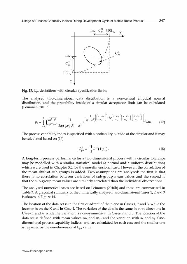
Fig. 13. Cpk definitions with circular specification limits
The analysed two-dimensional data distribution is a non-central elliptical normal distribution, and the probability inside of a circular acceptance limit can be calculated (Leinonen, 2010b)
2 2
2 2 2
2 2
12
2 1
42
1
2 1
Y YX X
X X Y Y
y m y mx m x mR
R x
R xR X Y
p e dxdy
. (17)
The process capability index is specified with a probability outside of the circular and it may
be calculated based on (16)
-1pk 4
11-
3RC p . (18)
A long-term process performance for a two-dimensional process with a circular tolerance
may be modelled with a similar statistical model (a normal and a uniform distribution)
which were used in Chapter 3.2 for the one-dimensional case. However, the correlation of
the mean shift of sub-groups is added. Two assumptions are analysed: the first is that
there is no correlation between variations of sub-group mean values and the second is
that the sub-group mean values are similarly correlated than the individual observations.
The analysed numerical cases are based on Leinonen (2010b) and these are summarised in
Table 3. A graphical summary of the numerically analysed two-dimensional Cases 1, 2 and 3
is shown in Figure 14.
The location of the data set is in the first quadrant of the plane in Cases 1, 2 and 3, while the
location is on the X-axis in Case 4. The variation of the data is the same in both directions in
Cases 1 and 4, while the variation is non-symmetrical in Cases 2 and 3. The location of the
data set is defined with mean values mX and mY, and the variation with sX and sY. One-
dimensional process capability indices and are calculated for each case and the smaller one
is regarded as the one-dimensional Cpk value.
www.intechopen.com

Systems Engineering – Practice and Theory
248
Y
USLX
LSLY
Tolerancecircle
LSLX
USLY
mX
mY
X
Example cases 1, 2 and 3
pdf of mY
pdf of mX
Fig. 14. A graphical representation of a two-dimensional process capability case-study
Case 1 Case 2 Case 3 Case 4
USL 0.45 0.45 0.45 0.45 LSL -0.45 -0.45 -0.45 -0.45 mX 0.225 0.225 0.225 0.225 mY -0.2 -0.2 -0.2 0.0 sX 0.05 0.025 0.05 0.05 sY 0.05 0.05 0.025 0.05
Distribution shape, main direction Circle Ellipse, y-axis Ellipse, x-axis Circle
1.50 3.00 1.50 1.50
1.67 1.67 3.33 3.00
Cpk = min (,) 1.50 1.67 1.50 1.50
Table 3. Input data for a two-dimensional process capability case study
The effects of statistical process models of the variation of the mean values of sub-groups in
the two-dimensional process performance index are simulated with Matlab with ten million
observations ordered into sub-groups with five observations within each sub-group. The
same process performance index name is used for both indices, whether based on the short-
or the long-term variation.
A significant effect of data correlation to the process’s capability may be seen in Figure 15,
which summaries the analysis of the example in Case 1. The X-axis is the correlation factor ρ
of the data set and the Y-axis is the value. The process capability index is calculated with a
numerical integration and simulated with a Monte Carlo-method without any variation of
the sub-groups for reference purposes (Leinonen, 2010b). The one-dimensional Cpk value is
1.5, and it may be seen that the two-dimensional process performance is maximised and
approaching 1.5 when the correlation of data rotates the orientation of the data set in the
same direction to that of the arch of the tolerance area.
www.intechopen.com

Usage of Process Capability Indices During Development Cycle of Mobile Radio Product
249
The statistical process models have a noticeable effect on the expected quality level. If the mean values of the sub-groups are varied independently, with a normal distribution in both the X and Y directions, the effect varies between 0.05 and 0.25. If the mean values vary independently with a uniform distribution in both directions, then the process model has a significant effect up to 0.45 to the with a correlation factor value of 0.6. If the maximum differences in values are converted to the expected quality levels, then the difference ranges from 13 dpm to 2600 dpm. The uniform distribution model suppresses the correlation of data more than normal distribution, and for this reason the long-term process performs worse. If the sub-group’s mean values are varied with normal distribution and correlated with the same correlation as the observations, then the long-term performance is a shifted version of the original process’s performance and the effect of the correlated process model on average is 0.1 units.
The results for Case 2 are shown in Figure 16. The variation in the X-axis direction is a half of the variation of the Y-axis direction and the one-dimensional Cpk value is 1.66. The two-dimensional index approaches the one-dimensional value when the correlation of data increases. If the correlation is zero, then the circle tolerance limits the process performance to 1.2 as compared with the one-dimensional specification at 1.66. If the mean values of the sub-groups are varied independently, either with a normal or a uniform distribution, the process performs better than with the correlated process model. In this case, the correlated mean shift model changes the distribution so that it points out more from the tolerance area than the uncorrelated models. It may be noted that when the correlation changes to positive, then the normal distribution model performs closer to the original process than the uniform distribution model.
-1 -0.8 -0.6 -0.4 -0.2 0 0.2 0.4 0.6 0.8 10.5
0.6
0.7
0.8
0.9
1
1.1
1.2
1.3
1.4
1.5
Rho
Cp
k(r
)
Closed form equation results for static process
Simulated results for static process
Mean value varied with correlated N distribution
Mean value varied indepenently for X and Y with N distribution
Mean value varied independently for X and Y with U distribution
Fig. 15. The effect of the variation of the mean value of sub-groups on a two-dimensional , Case 1
www.intechopen.com

Systems Engineering – Practice and Theory
250
-1 -0.8 -0.6 -0.4 -0.2 0 0.2 0.4 0.6 0.8 10.8
0.9
1
1.1
1.2
1.3
1.4
1.5
1.6
Rho
Cp
k(r
)
Closed form equation results for static process
Simulated results for static process
Mean value varied with correlated N distribution
Mean value varied indepenently for X and Y with N distribution
Mean value varied independently for X and Y with U distribution
Fig. 16. The effect of the variation of the mean value of sub-groups on a two-dimensional ,
Case 2
The example of Case 3 shows half of the variation in the Y-axis direction as compared with the X-axis direction, and the one-dimensional Cpk value is 1.50. The results for Case 3 are presented in Figure 17. If the sub-group mean values are varied with correlated normal distributions, then the process capability with negative correlations is the best since the correlated process model maintains the original correlation of the data. The uncorrelated normal distribution has an overall data correlation between -0.8 to 0.8, and the uncorrelated uniform distribution has a correlation between -0.57 and 0.57. The uncorrelated uniform distribution model has an effect from 0.25 up to 0.42 of the value.
The results for the Case 4 are presented in Figure 18. The example provided by Case 4 has a symmetrical variation and the distribution is located along the X-axis. For these reasons, the correlation has a symmetrical effect on the two-dimensional process performance indices. The one-dimensional Cpk value is 1.50 and the close form equation result without the correlation has a value of 1.45. Both normally distributed process models have a value of 1.31 with the correlation factor at zero. The correlated process model differs from the uncorrelated one with high correlation factor values. The uniform distribution model clearly has the biggest impact on the estimated quality level up to 0.3. The process performance indices maintain the order of the quality level estimations over the correlations due to the symmetrical distribution and location.
As a conclusion, it is not possible to derive similar easy-to-use process capability indices, including the effects of the statistical process models of two-dimensional process performance indices as compared with one-dimensional ones based on the results presented in Chapter 3.2.
www.intechopen.com

Usage of Process Capability Indices During Development Cycle of Mobile Radio Product
251
-1 -0.8 -0.6 -0.4 -0.2 0 0.2 0.4 0.6 0.8 1
0.7
0.8
0.9
1
1.1
1.2
1.3
1.4
1.5
Rho
Cp
k(r
)
Closed form equation results for static process
Simulated results for static process
Mean value varied with correlated N distribution
Mean value varied indepenently for X and Y with N distribution
Mean value varied independently for X and Y with U distribution
Fig. 17. The effect of the variation of the mean value of sub-groups on a two-dimensional , Case 3
-1 -0.8 -0.6 -0.4 -0.2 0 0.2 0.4 0.6 0.8 11
1.05
1.1
1.15
1.2
1.25
1.3
1.35
1.4
1.45
1.5
Rho
Cp
k(r
)
Closed form equation results for static process
Simulated results for static process
Mean value varied with correlated N distribution
Mean value varied indepenently for X and Y with N distribution
Mean value varied independently for X and Y with U distribution
Fig. 18. The effect of the variation of the mean value of sub-groups on a two-dimensional , Case 4
www.intechopen.com
Systems Engineering – Practice and Theory
252
4. Usage of process capability indices in radio engineering
Most of the parameters which are studied during the RF system design phase do not follow a normal distribution. Monte Carlo-simulations have been carried out for the most important RF block level parameters and - based on the simulations results - none of the RF block level parameters follow a normal distribution (Vizmuller, 1998). This is due to fact that the dynamic range of signal levels in radio engineering is huge and typically a logarithm scale is used for signal levels. Unfortunately, in most cases the signal levels do not follow a normal distribution on such a scale. In order to perform a process capability analysis properly for radio engineering parameters, the analysis should be done according to specific distributions, as shown in Figure 5. If a production quality level estimation of an RF parameter is done based on a process capability index with a normal distribution assumption, then the quality level may be significantly under- or overestimated. The problem is that the underlying distributions for all important RF parameters are not available or known and the analyses are based on measured results. The problem with a measurement-based approach is that the properties of the data distributions may change during the development cycle of the device.
Another problem with a measurement-based approach for process capability analysis is that a measurement error of an RF parameter may change the properties of the data distribution. The measurement error based on the RF test equipment on the process capability indices has been studied (Moilanen, 1998). Based on the study of the effect of RF, test equipment needs to be calibrated out and the analysis should be done with actual variation which is based on product-to-product variation. An actual number of RF measurements cannot be reduced based on mathematical modelling, since most RF parameters do not follow the normal distribution and the accuracy of the modelling is not good enough for the purposes of design verification or process capability analysis (Pyylampi, 2003).
Some work has been done in order to find the underlying functions for some critical RF
parameters. The statistical properties of the bit error rate have been studied and a statistical
distribution of it would follow an extreme value function on a linear scale or else it would
follow a log-normal distribution on a logarithm scale with a DQPSK modulation (Leinonen,
2002). In order to validate this result in real life, an infinitive measurement result and
measurement time would be needed. It has been shown that, based on measurement results,
a peak phase error of a GSM transmission modulation would follow - statistically - a log-
normal distribution (Leinonen, 2002). The statistical distribution of a bit error rate of a QPSK
modulation has been studied and, with a limited measurement time and measurement
results, the distribution of the bit error rate is a multimodal distribution (Leinonen, 2011).
The multimodal distribution has a value of zero and a truncated extreme value function
distribution part on a linear scale or else a truncated extreme value function distribution on
a logarithm scale. Based on the previous results, the process capability analysis of the bit-
error rate based on known statistical distribution functions has been studied (Leinonen,
2003, 2011).
Process capability indices give an indication of the maturity level of the design even though the process capability indices may over- or underestimate the expected quality level. The maturity levels of multiple designs may be compared to each other, if the calculation of the indices has been done in a similar manner.
www.intechopen.com

Usage of Process Capability Indices During Development Cycle of Mobile Radio Product
253
Process capability indices are used as a communication tool between different parties during the development process of the device. Different notation for the process capability index may be used in order to create differences between a process capability index based on a normal distribution or those based on a known or non-normal distribution assumption. One proposal is to use the C*pk notation if the process capability index is based on non-normal distribution (Leinonen, 2003).
Typically, the studied parameters during the RF system engineering and R&D phases are one-dimensional parameters, and multiradio interoperability may be considered to be one of the rare two-dimensional RF design parameters. Multiradio interoperability in this context is considered to be purely defined as a radio interference study, as shown in Figure 4. Multiradio interoperability may be monitored and designed in the manner of a process capability index (Leinonen, 2010a). A new capability index notation MRCpk has been selected as a multiradio interoperability index, which be defined in a manner similar to the process capability index in equation 16, at least for communication purposes. In order to make a full multiradio interoperability system analysis, all potential interference mechanisms should be studied. A wide band noise interference mechanism has been studied with an assumption that the noise level is constant over frequencies (Leinonen, 2010a). Typically, there is a frequency dependency of the signal level of the interference signals and new studies including frequency dependencies should be done.
The effects of statistical process models on normally distributed one- and two-dimensional data has been studied in 3.2. and 3.4. Unfortunately, most of RF parameters are, by nature, non-normally distributed and thus previous results may not apply directly. More studies will be needed in order to understand how simple statistical process models will affect non-normally distributed parameters. If the manufacturing process could be taken into account more easily during the system simulation phase, either block level or component level specifications could - potentially - be relaxed. If the manufacturing process cannot be modelled easily, then the block level and component level specifications should be done in a safe manner which will yield the over-specification of the system. If the system or solution is over-specified, the solution is typically more expensive than the optimised solution.
5. Conclusion
In high volume manufacturing, the high quality level of the product is essential to maximise the output of the production. The quality level of the product needs to be designed during the product development phase. The design of the quality begins in the system definition phase of product development by agreeing upon the most important parameters to follow during the development phase of the device. Block level and component level specifications are defined during the system engineering phase. The actual specifications and how they are specified are main contributors towards the quality level of the design.
The maturity and potential quality level of the design may be monitored with process capability indices during the product development phase. The process capability indices had originally been developed for the quality tools for manufacturing purposes. Multiple parameters may be compared to each other, since process capability indices are dimensionless, which is an advantage when they are used as a communication tools between technology and quality teams.
www.intechopen.com

Systems Engineering – Practice and Theory
254
Components may be defined using previous information regarding the expected variation of the parameter or based on the calculation and simulation of the parameters. If the component specifications are only defined when based on calculations and simulations, then the variability of the manufacturing of the component and a variability of a device’s production need to be taken into account. The manufacturability margin for parameters needs to be included, and one method for determining a needed margin is to use statistical process variation models. Statistical process control methods are used in high volume production and they allow the actual production process to vary between the control limits of statistical control charts. The control limits of the control charts are dependent on a number of samples in a sample control group, and the control limits define the allowable process variation during mass production. A constant mean shift process model has been used in a Six Sigma community to model mass production variation. The effects of a constant process shift model and normal distribution- and uniform distribution-based process models are compared with each other and with the one-dimensional normally distributed data. Based on the simulation results, the constant shift and the uniform distribution models expect a similar quality level with a process capability index value of 2, while at a lower process capability level a constant shift process estimates the lowest quality level. The normal distribution model of the manufacturing process expects a higher quality level than other process models with a one-dimensional parameter. New equations for one-dimensional process capability indices with statistical process models based on calculations and simulations have been presented in the Chapter 3.2.
Process capability indices have been defined according to multidimensional parameters
which are analogous to one-dimensional process capability indices. One of the main
differences between one- and two-dimensional process capability index analyses is that a
correlation of the data with two-dimensional data should be included into the analysis.
Another difference is the definition of the specification limit, which may be rectangular or
circular or else a sub-set of those. A rectangular tolerance area may be considered if the two-
dimensional data is uncorrelated, and the specifications may be considered to be
independent of each other. Otherwise, the tolerance area is considered to be circular. The
effects of statistical process models for two-dimensional process capability indices with a
correlated normal distribution with a circular tolerance area have been studied. The
correlation of the data has a significant effect on the expected quality level based on the
simulation results. The location and the shape of the data distribution have an additional
effect when statistical process models are applied to the data. Easy to use equations which
take the statistical process models into account with two-dimensional data cannot be
derived due to multiple dependences in terms of location, shape and the correlation of the
data distribution.
Most radio performance parameters are one-dimensional and they are not distributed with a
normal distribution, and so the process capability analysis should be carried within known
statistical distributions. A process capability analysis based on a normality assumption may
significantly under- or overestimate the expected quality level of the production. The
statistical distributions of some RF parameters are known - e.g., the bit error rate - but more
work will be needed to define the others. Also, a multiradio interoperability may be
considered to be a two-dimensional parameter which may be analysed with process
capability indices.
www.intechopen.com

Usage of Process Capability Indices During Development Cycle of Mobile Radio Product
255
6. References
Albing, M. (2008). Contributions to Process Capability Indices and Plots, Doctoral thesis, Luleå University of Technology, ISSN 1402-1544
Bissell, A. F. (1990). How reliable is Your Capability Index? Applied Statistics, Vol. 39, No. 3, pp.331-340
Breyfogle, F. (1999). Implementing Six Sigma: Smarter Solutions Using Statistical Methods, John Wiley & Sons, ISBN 0-471-29659-7, New York, USA
Clements, J. A. (1989). Process Capability Calculations for Non-normal Distribution, Quality Progress, pp. (95-100), ISSN 0033-524X
Gartner Inc., (February 2011) Competitive Landscape: Mobile Devices, Worldwide, 4Q10 and 2010, 11.8.2011, abstract available from:
http://www.gartner.com/it/page.jsp?id=1543014 Kotz, S. & Johnson, N. L. (2002). Process Capability Indices – A review, Journal of Quality
Technology, Vol. 34, No 1, pp.2-19 Kotz, S. & Johnson, N. L. (1993). Process capability indices, Chapman & Hall, ISBN 0-412-
54380-X, London, UK Leinonen, M. E. (1996). The Yield Analysis of RF blocks with Cpk method, Diploma Thesis,
University of Oulu, p.60, in Finnish Leinonen, M. E. (2002). The Statistical Analysis of RF Parameters in GSM Mobile Phones,
Licentiate Thesis, University of Oulu, p.121. Leinonen, M. E. (2003). Process Capability Index Usage as a Quality metric of Digital
Modulation Receiver, Proceedings of URSI/IEEE XXVIII Convention of radio science & IV Finnish Wireless Communication Workshop, pp.50–53, Oulu, Finland, October 16-17, 2003
Leinonen, M. E. (2010,a). Multiradio Interoperability index, Proceedings of 3rd European Wireless Technology Conference, pp.145-148, ISBN: 972-2-87487-018-7, Paris, France, September 27-28, 2010
Leinonen, M. E. (2010,b). The Effect of Data Correlation to Process Capability Indices in Position Tolerancing, Proceedings of ISSAT2010 Conference, pp.21-25, ISBN: 978-0-9763486-6-5, Washington, USA, August 5-7, 2010
Leinonen, M. E. (2011). Process Capability Index Analysis of Bit Error Rate of QPSK with Limited Observations, to be presented at 41st European Microwave Conference, Manchester, United Kingdom, October 9-14, 2011
Lu, M. & Rudy R. J. (2002). Discussion. Journal of Quality technology, Vol. 34, No 1, pp.38–99 Harry, M. & Schroeder, R. (2000) Six Sigma the Breakthrough Management Strategy
Revolutionizing the World's Top Corporations, Random House, ISBN 0-385-49438-6, New York, USA
Moilanen, T. (1998). The Error Determination which Comes from Measurement Equipment during Mobile Phone RF Measurements, Engineering Thesis, Polytechnic of Ylivieska, 63 p., in Finnish
Montgomery, D. C. (1991). Introduction to Statistical Quality Control, 2nd ed., John Wiley & Sons, Inc., USA
Pearn, W.L. and Chen, K. S. (1999) Making decisions in assessing process capability index Cpk. Quality and Reliability engineering international, Vol. 15, pp.321-326
Pyylampi, K. (2003). The Mathematical Modelling of RF parameters in GSM phone, Diploma Thesis, University of Oulu, p.63, in Finnish
www.intechopen.com

Systems Engineering – Practice and Theory
256
Uusitalo, A. (2000). The Characterization a Long Term Process Deviation for RF Parameters in high volume Mobile Phone Production, Engineering Thesis, Polytechnic of Oulu, p.45, in Finnish
Vizmuller, P. (1998). Design Centering Using Mu-Sigma Graphs and System Simulation, Artech House, ISBN 0-89006-950-6, Norwood, MA
Wu C.-H., Pearn W. L. & Kotz S. (2009) An Overview of theory and practice on process capability indices for quality assurance. Int. Journal Production Economics, 117, pp.338 - 359
www.intechopen.com

Systems Engineering - Practice and TheoryEdited by Prof. Boris Cogan
ISBN 978-953-51-0322-6Hard cover, 354 pagesPublisher InTechPublished online 16, March, 2012Published in print edition March, 2012
InTech EuropeUniversity Campus STeP Ri Slavka Krautzeka 83/A 51000 Rijeka, Croatia Phone: +385 (51) 770 447 Fax: +385 (51) 686 166www.intechopen.com
InTech ChinaUnit 405, Office Block, Hotel Equatorial Shanghai No.65, Yan An Road (West), Shanghai, 200040, China
Phone: +86-21-62489820 Fax: +86-21-62489821
The book "Systems Engineering: Practice and Theory" is a collection of articles written by developers andresearches from all around the globe. Mostly they present methodologies for separate Systems Engineeringprocesses; others consider issues of adjacent knowledge areas and sub-areas that significantly contribute tosystems development, operation, and maintenance. Case studies include aircraft, spacecrafts, and spacesystems development, post-analysis of data collected during operation of large systems etc. Important issuesrelated to "bottlenecks" of Systems Engineering, such as complexity, reliability, and safety of different kinds ofsystems, creation, operation and maintenance of services, system-human communication, and managementtasks done during system projects are addressed in the collection. This book is for people who are interestedin the modern state of the Systems Engineering knowledge area and for systems engineers involved indifferent activities of the area. Some articles may be a valuable source for university lecturers and students;most of case studies can be directly used in Systems Engineering courses as illustrative materials.
How to referenceIn order to correctly reference this scholarly work, feel free to copy and paste the following:
Marko E. Leinonen (2012). Usage of Process Capability Indices During Development Cycle of Mobile RadioProduct, Systems Engineering - Practice and Theory, Prof. Boris Cogan (Ed.), ISBN: 978-953-51-0322-6,InTech, Available from: http://www.intechopen.com/books/systems-engineering-practice-and-theory/usage-of-process-capability-indices-during-development-cycle-of-mobile-radio-product