U.S.A. the Fast Food Nation:Obesity as an Epidemic

Arlene M. Evangelista∗, Angela R. Ortiz†, Karen R. Rıos-Soto‡, Alicia Urdapilleta§

Abstract

The prevalence of overweight and obesity has increased dramatically inthe Unites States. Obesity has become a disease of epidemic proportions. Infact, 1 out of 3 people in the United States are obese. Fast-food accessibil-ity is partly to blame for observed patterns of obesity and overweight. Theaim of this project is to study the potential role of peer-pressure in fast-foodconsumption as well as its effect on an individual’s weight. We explore theseeffects on the dynamics of obesity at the population level using an epidemio-logical model. In this framework, we can explore the impact of interventionstrategies. Statistical data analysis provides insights on the relation betweendemographic factors and weight.

1 Background

Major world organizations such as the American Obesity Association, National Insti-tutes of Health, World Health Organization, American Heart Association, all agreeon one thing: obesity is growing at an alarming rate and is now a serious disease ofepidemic proportions. Since 1980, obesity rates in U.S have increased by more than60% in adults, while rates have doubled in children, and tripled in adolescents [16].According to the Center for Disease Control and Prevention, obesity is defined as“the excessively high amount of body fat or adipose tissue in relation to lean bodymass” [8]. Some of the “identifiable signs and symptoms”of obesity include: excessaccumulation of fat, increased levels of glucose, as well as increased blood pressure,

∗Arizona State University†Arizona State University‡Cornell University, Ithaca, NY 14853§Arizona State University

81

and cholesterol levels [3]. Obesity is assessed and measured using the Body MassIndex (BMI), which is a number calculated using the individual’s height and weight.Individuals are considered underweight if their corresponding BMI falls below 18.5,normal weight if their BMI falls between 18.5-24.9, overweight if their BMI fallsbetween 25.0-29.9, and obese if their BMI falls above 30.0 [8]. Hence, classificationof individual’s weight depends on their BMI.

In general, there exists several factors that play a role in body weight, andtherefore, in becoming obese. These factors include an individual’s environment,behavior, metabolism, culture, genes, and socioeconomic status. The rapidity withwhich obesity rates have increased in the U.S, and even worldwide can be attributedto the previous factors. In particular, the increased U.S obesity rates can predomi-nantly be explained by changes in the individual’s behavior and environment. Thisis because in the last 20 years, people have modified their calorie intake and energyexpenditure as well as reduced their physical activity ([16],[11],[27]). In 1977 theproportions of meals consumed away from home was 16%, by 1987 that proportionrosed to 24%, and by 1995 to 29%. In 1977, Americans got 18% of their totalcalories intake away from home, and fast food places accounted for 3% of the totalcalorie intake. By, 1994 total calorie intake away from home rose to approximately34%, while fast food calorie intake rose to 12% by the year 1997. By 2002, fast foodconsumption accounted for more than 40% of a family’s budget spent on food [11].The reduced physical activity of individuals and increased consumption of energyintake, can be also be attributed to the family’s hectic work and schedules. In ad-dition economic growth, urbanization and globalization of food markets are some ofthe forces that have contributed to the development of obesity as an epidemic.

When considering the world population, the World Health Organizations, alsoreports that roughly one billion adults worldwide are overweight and around 300 mil-lions of these are considered clinically obese [27]. In addition, 17.6 million childrenunder five years are consider to be overweight worldwide. Hence, this problem isglobal and it affects both industrialized (developed) and developing countries. Theepidemic of obesity is making such a negative impact that is has also been associ-ated with other fatal and non-fatal diseases. For example, nonfatal diseases include:respiratory difficulties, arthritis, infertility and psychological disorders(depression,eating disorders, and low self-esteem). Fatal diseases include: diabetes, heart at-tacks, blindness, renal failure and certain type of cancers. ([8],[9]). By 2002, it wasestimated that obesity accounted for 300,000 deaths in U.S annually. Furthermore,by this same year, it was estimated that obesity and its complications were alreadycosting the nation about $117 billion annually, of the $1.3 trillion spent on health

82

care each year ([16], [21]).

2 Introduction

According to the Center for Disease Control (CDC), approximately 64% of U.Sadults and 15% of children and adolescents are overweight. In 2002, obesity wasthe second cause of preventable deaths after smoking [9]. Major organizations suchas the World Health Organization and National Institute of Health as well as othersources ([16],[11],[27]) indicate that an increase of energy intake, and nutrient poorfoods with high levels of saturated facts, and sugars is partly to blame for theincreased number of overweight and obese individuals [1]. Today, Americans areconsidered to be the fattest people in the world after the Sea Islanders ([11], [1],[23]). A study on the effects of fast food consumption among children also foundthat fast food could be one of the factors for the increased prevalence of obesity inchildren. It was found that children who ate fast food consumed more total andsaturated fat, more carbohydrates, sugar and less dietary fiber, milk, fruit and veg-etables. Of the 6,212 children and adolescents, 30% ate fast food any given day, andthey ate an average of more than 187 calories per day than those children who didnot ate fast food. These additional calories per day can account for an extra sixpounds per year ([4],[10]).

The first motivation for this work came from a stronger link observed betweenthe effects of fast food and obesity in a documentary, called “Super Size Me”. Inthis documentary, a typical individual, Morgan Spurlock, films himself eating all 3meals per day for 30 days at Mc’Donald restaurants. At the end of the 30 days,Spurlock not only gained 20 pounds, but he had high levels of cholesterol and highblood pressure [24]. Throughout the years, the food marketing industry has suc-ceeded in making people consume more and more. Most fast food restaurants can“Size it your way”, i.e., you can have a medium, large or king-sized value meal. Byordering items together, and by super sizing their value meal, people save an averageof 78 cents, but for this 78 cents people get a 200 to 250 increased calorie intake([22]). Surprisingly, U.S residents spend more money on fast food than they spendon movies, books, magazines videos and records combined. In 1970, Americans werespending $6 billion on fast food, and by the year 2000, Americans were spending$110 billions ([1], [23]).

Fast food industry has not only transform the American diet, but the landscape,economy, workforce, and popular culture. Fast food is relative “good” in taste, in-

83

expensive and convenient that it has become a “common place that it has acquiredan air of inevitability, as though it were somehow unavoidable, a fact of life” [23].Statistics show, that on any given day, 1/4 of the adult population visits a fast foodrestaurant [23]. Millions of people buy fast food everyday, supersizing their valuemeals thinking they are saving money and time without thinking of the actual costof super sizing their value meal: gaining weight. Thus, because of the increasingnumber of overweight and obese individuals (adults, adolescents, and children) andthe detrimental non-fatal and fatal consequences of obesity, for this project, we areinterested in analyzing the dynamics of fast food consumption and obesity in the U.Spopulation using an epidemiological model. In particular, the aim of this projectis to study the potential role of peer pressure in fast food consumption as well asits effect on individual’s weight. We developed a mathematical model, with specialcases, to analyze the progression rate from normal weight individuals(N) to over-weight (O1) and obese(O2) individuals. The classification of N , O1, O2 individualsis based on their BMI. The progression from normal to overweight individuals ismeasured by incorporating a peer pressure, β, by which individuals start eating atfast food restaurants. People start eating at fast food restaurants not only becauseother people invite them to come along but because of socio-economic status, ac-cessability and convenience to fast food restaurants.

This paper is divided as follows: background and introduction are given onsections 1 and 2. Section 3 includes the statistical analysis on the demographicfactors with the individuals weight. Section 4 introduces the obesity model, whilein section 5 and 6 two special cases of this model are presented. Section 7 includesensitivity analysis while section 8 have the parameter estimation. Section 9 supportthe analysis of the obesity model through numerical simulations. Finally section 10concludes our work.

84

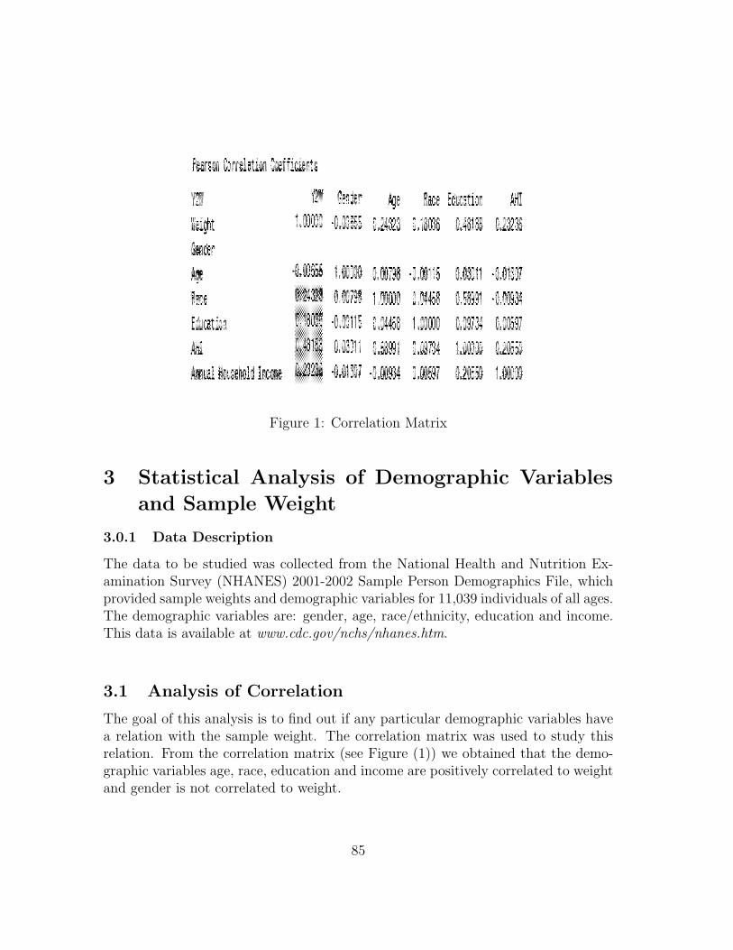
Figure 1: Correlation Matrix

3 Statistical Analysis of Demographic Variablesand Sample Weight

3.0.1 Data Description

The data to be studied was collected from the National Health and Nutrition Ex-amination Survey (NHANES) 2001-2002 Sample Person Demographics File, whichprovided sample weights and demographic variables for 11,039 individuals of all ages.The demographic variables are: gender, age, race/ethnicity, education and income.This data is available at www.cdc.gov/nchs/nhanes.htm.

3.1 Analysis of Correlation

The goal of this analysis is to find out if any particular demographic variables havea relation with the sample weight. The correlation matrix was used to study thisrelation. From the correlation matrix (see Figure (1)) we obtained that the demo-graphic variables age, race, education and income are positively correlated to weightand gender is not correlated to weight.

85

Pearscfl

~e Race tdocatiar [,24~3 ;,16036 ~,2~3C

Gende~

A;~ -0,0100) ~, 00i98

~ace 1,00000 ;,[r.1458 Q,58l91 -Q,OOOai 0, l,[r.1q56 1,00000 O,O91~

r \800' ;,;, ) ; ,00;34

':lLsenold IrcCIle '00934

3.2 Exploratory Analysis of Possible Interactions of Demo-graphic Variables and Sample Weight

3.2.1 Methodology

The goal of this analysis is to find out if any particular demographic variables have anindividual effect with weight or if its effect depend on the level of other demographicvariable. A versatile statistical tool to study this relation is the analysis if variance(ANOVA). The starting model to be analyzed contains factor effects as well as allpossible combinations of interaction factor effects. To analyze this model a SASprogram was created (see Appendix) to produce the ANOVA table that decomposesthe total variation in the data, as measured by the Total Sum of Square (TSS), intocomponent that measure the variation of each factor, a components that measure thevariation given each factor interaction and the error sum of square (ESS). The tablealso gives the F-statistic values and the p-values of these components for testingeffects. The SAS program created two tables, Type I SS and Type III SS. TypeIII SS is used for unbalanced factor sample size. The fact that some demographicfactors contain missing values implies that we have an unbalanced factor samplesize, then the ANOVA table Type III SS will be used. In order to test the factorand interaction effects, we can use the p-values from the obtained table. Sincein this type of study we do not need to be too precise, a level of significance of5% is used. Any p-value of each factor and interaction effect that falls below thislevel of significance is considered statistically significant. After concluding, with thesignificant effects, a ANOVA model is suggested. We emphasize the importance ofexamining the appropriateness of the ANOVA model under consideration, so anyinference made with this model can be valid. This appropriateness of the modelcan be determined from the residual analysis. This residual analysis is carried outby the normal score plot of the residual to determine normality of the residuals,the residual versus fitted value to determine constancy of error variance and thepresence of outliers; and the distance of variance plot (Cook’s distance) to determineinfluential outliers observations. The reason why the normality assumption is thatthe estimator and testing procedure are based on t-distribution which is sensitive tolarge departures from normality.

3.2.2 Results

Analyzing the SAS output (see Table (1)), we obtained that there is: age (group)main effect with a p-value < 0.0001, race main effect with a p-value < 0.0001,education main effect with a p-value < 0.0001 and income main effect with a p-value of 0.0059. There are two-factor interaction effects between age-race with a

86

Figure 2: Interaction Plot: Existence of Interaction

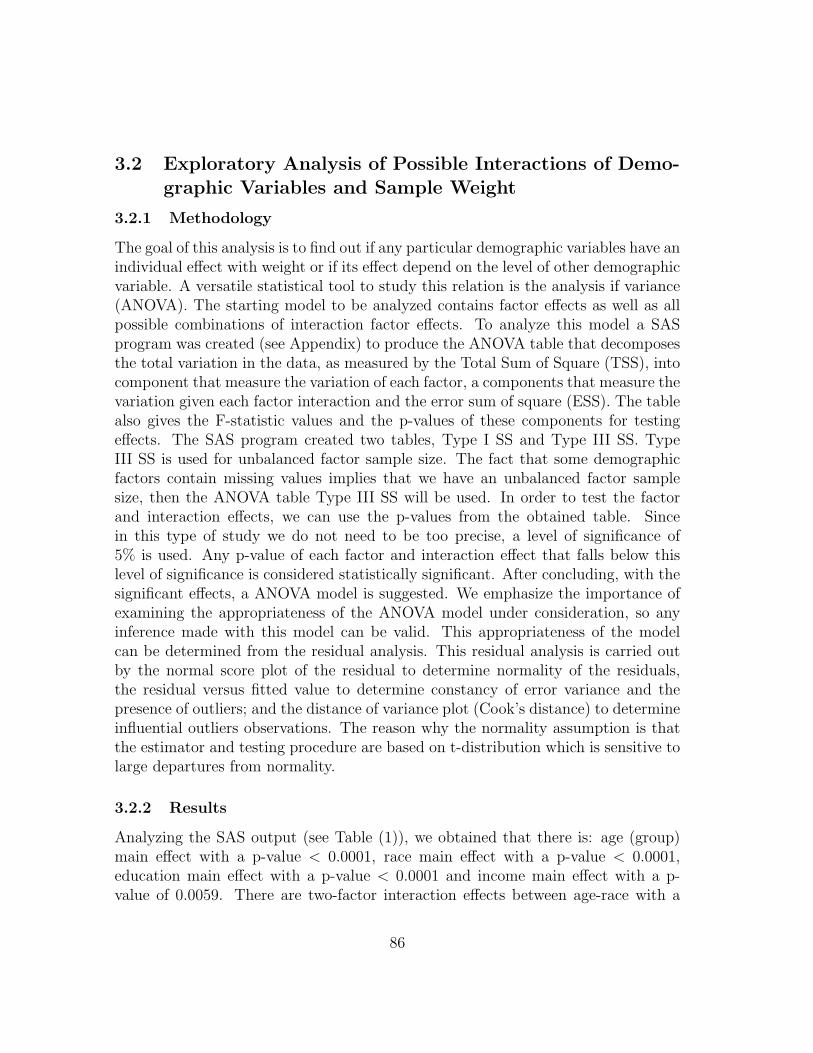
p-value of < 0.0001, between age-education with a p-value < 0.0001, between race-education with a p-value of < 0.001 and between race-income with a p-value of0.0002. There are three-factor interaction effects between age-race-education witha p-value of 0.0022, between age-race-income with a p-value < 0.0001 and betweenrace-education-income with a p-value 0.0008. Also, weak four-factor interactioneffect between age-race-education-income is found because the p-value of 0.0500.Some examples of the existence and no existence of interactions are show in Figure(2) and Figure (3).

The five-factor ANOVA model is:Y = µ.. + α Age + β Race + γ Education + ρ Income + (αβ) Age*Race + (αγ)Age*Education + (βγ) Race*Education + (βρ) Race*Income + (αργ) Age*Race*Education+ (αβρ) Age*Race*Income + (βγρ) Race*Education*Income.

Here µ.. means the the overall mean weight. The age main effect implies thatfor each age level, the mean weight is statistically significant different form theother. The same interpretation applies to the main effects for race, education andincome. The two-factor interactions implies that for each two level combinationthe mean weight is statistically significant different from the other. Finally, thesame interpretation can be given to the three-factor interactions for each three level

87

Interaction Plot between Race and Educaton

~ : ; m ,---------;;------------------------,

111 11

HI li

Jl III

I", I h " [i ,, e-tl-tl EH3-!3 1 I>-i>-i> I e-tl-tl , e-tHl]

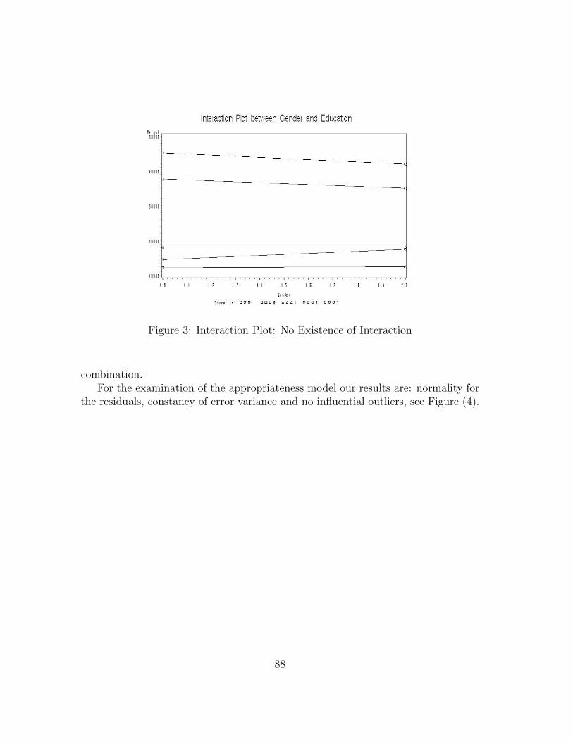
Figure 3: Interaction Plot: No Existence of Interaction

combination.For the examination of the appropriateness model our results are: normality for

the residuals, constancy of error variance and no influential outliers, see Figure (4).

88

Interaction Pht ootiieen Gender and Education , ,

411 1 ,

JIl l ,

!II I ,

1111 , "

, , " " " " " " " " "

I"j" [h,.l i, . &-<HI !HHl 1 ~ I eo-tHl1 e-+e j

Tab

le1:

AN

OVA

Tab

le

89

Ii' Ii' Ii' if Ii' Ii' if Ii' Ii' Ii' l Ii? fj' Ii' Ii' Ii' ~ l l if Ii? Ii? Ii' Ii' Ii' Ii' ~ ~ l Ii? Ii' 8' Ii' ~ ~~ ~ ~~ ~ ~~~ ~~~ ~~~~ ~~~~~ ~~~~ -~~~ ~~i "..I ~ "~..I"~~~ . .., .. ~~~ ~ .. "",,~~~~ ~ ..,~n! d~~~~~ ~ 1'1~~~'11~~~' ~ ~1"1 = ,~ ~~~~d~~l~ l~~~ ififif9 -~ ~~~~~lif 9 ~ ~"'.~. ~.~~ ~~~ ~~~. ·. SSS · ~ ~~-~~S . """'" .~".~ . ~. ' ''' '''',,~ ~ " ~" ~~~ ~ l~;~=~g_~'~~- g ~ = ~ ~~~~m ~. ~g- ~ ~ ~~ ~ ~ g ~~ ! !!~~e! - ~ ~ ~ ______ 0 _ , ~

, , i ,

iii:!! ~ ~ fl "' :!!;;; ~.!!:::; i!.:!! '" .,Il .\';;;; ti "''' =" .. '" '" " • .. "' - ~>§:

",," - ,, _ '"'' "',,," - .... '" "'''''"" .... - .. ! " i -"" ~"!'" ,-"" -" " -"' !' 1:! _ t>l~ _ $x ___ .... ij;<I!!i!"'e; _ '"!!l"':I!:t: _ ~ I: ~~ :;:i ~ ~ (I ~ is g: 8l2l ~ Rl ~ III il ~ 0;;;;$ OJ = ~ Ii ~ ffi t>l ~ & ~ ;; ~!'i . ~

~ ~ f! ~ ~ ~ ~ ~ ~ is 8l ~ ~ ~ ~ ~ ~ 0; 13 ~ ~ ~ ~ ~ ~ ~ ~ ~ ~ ~ ~ B •• 1. _, ... I I, .. ,. ill .. _ .• • _. 1 •• 1. '"" 0 _ ........ _ .. '" '" '" ~ ........ .. ...... .... "" .. ... " _ ., "' .. _ '" '"

~ ~ ~ i ~ ~ ~ ~ ~ ~ ~ ~ ~ ~ i ~~ ~ t>l £ i ~ g; ~ ~ ~ ~ ~ ~ ~! ! I I I ~ i! ~!! ~ Ii, . I! !!! iii" i i!.I :: ~~ ~ ~g:~~~~~~!'i8~~~gRl~~~ ~ ~8l!'i8;;;8lg:8l~~ tll ~ ;, ~ "' ~ '" ;, ;" ;" :... :.. " Co ::: :.. ;" :.. ~ ;" :- !Ii :.. :... :.. ;" " ~ ~ ~ ;:j ~ " ... "' ... "''' '" '" -" ... '" "' ... '" "'''' ... .o. '" _ .o. '" "''' '" "' ... '" '" '" ~

, _ "''"'" <

pp pppp p !" PPP:- ?' P?' PPPP ro,,?' ~ p ~

:0: '" tl1 ~ ~ ;;; t3 S! <l!i! !l ;:j £ 8l;3 ~~ $ ~ I!l tl1 jS SlI3 't. ij ~ !:lSl 8 ~

o 0000000'000000'0"00000"'0 "" . . . . . . . . . . . . . .. ............. ~

§ § § § ~ § § ~ § ~ § § § ~ ~ i~ § § i § § ~ ~ ~ ~ § § § § § ~

-

o. ,. " " ,. .. I, .,

" " ::: !il . ' , ~

'. , . o •

g ~ !f8' ~ d !i" ~ a ' ... ~ , i •

", ill !Hl ~

••• ~~~

~~~i 1511Hl ~ ~ """no ,

". i~~ !il ~-!! , . _. , ...

, ~ ~

" " o ' , . "

, , ! , , , i , • " -

l ~"ii'!i'C ·1'1 .. - , ,

~nif ! So ;:; ... ~ • '" ",,,,,,:;~i:

c , ., S < ~ ~ ~-o---~"'a ~"'-"'''''''~ ... ~ ~""''''' n~ g ... '" : I . . -· , , . o.

I-o

• •

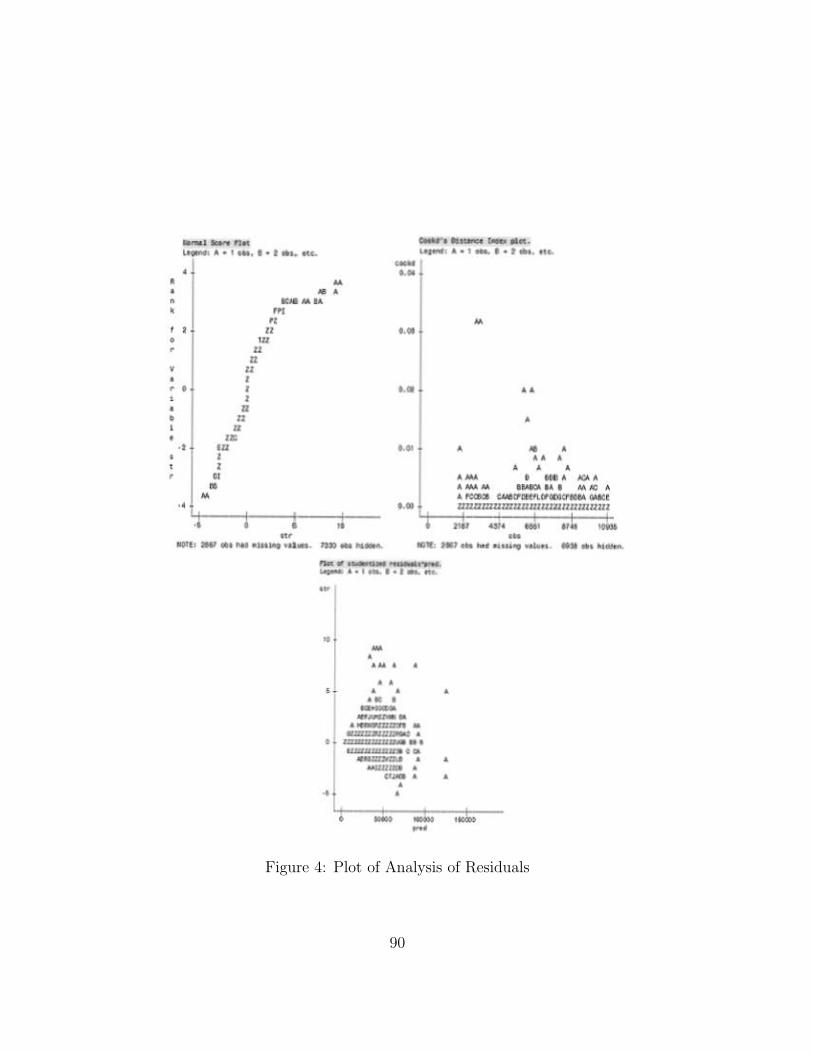
Figure 4: Plot of Analysis of Residuals

90

-, ........ - ',--_. _.· '_.1· .-.. .... _ .· '_1 .. _ ..... -• o. • • • • • • _ .. • rn

" • • " , . • • • " " ,

" , • , 0 o. .. 0

• " , " • , • • o. ., ,. o. • • • 0 .. •

0 • • • • " .- , -' -' • ._ . _., o. • • . - -....... __ ..... . , , .• muomllm"""'U..,"UmUI"

• • - - •• -•• -... ,--_ ....... . .-.. --- •• -_ ... .. -.. - . _ ... .. -••

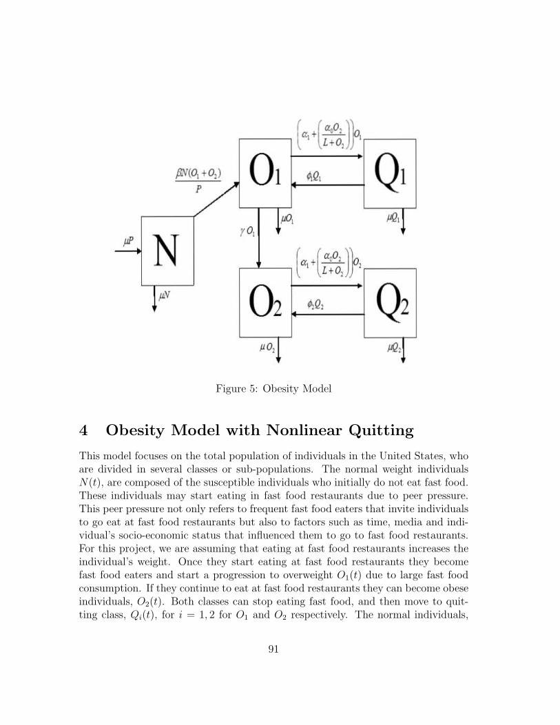
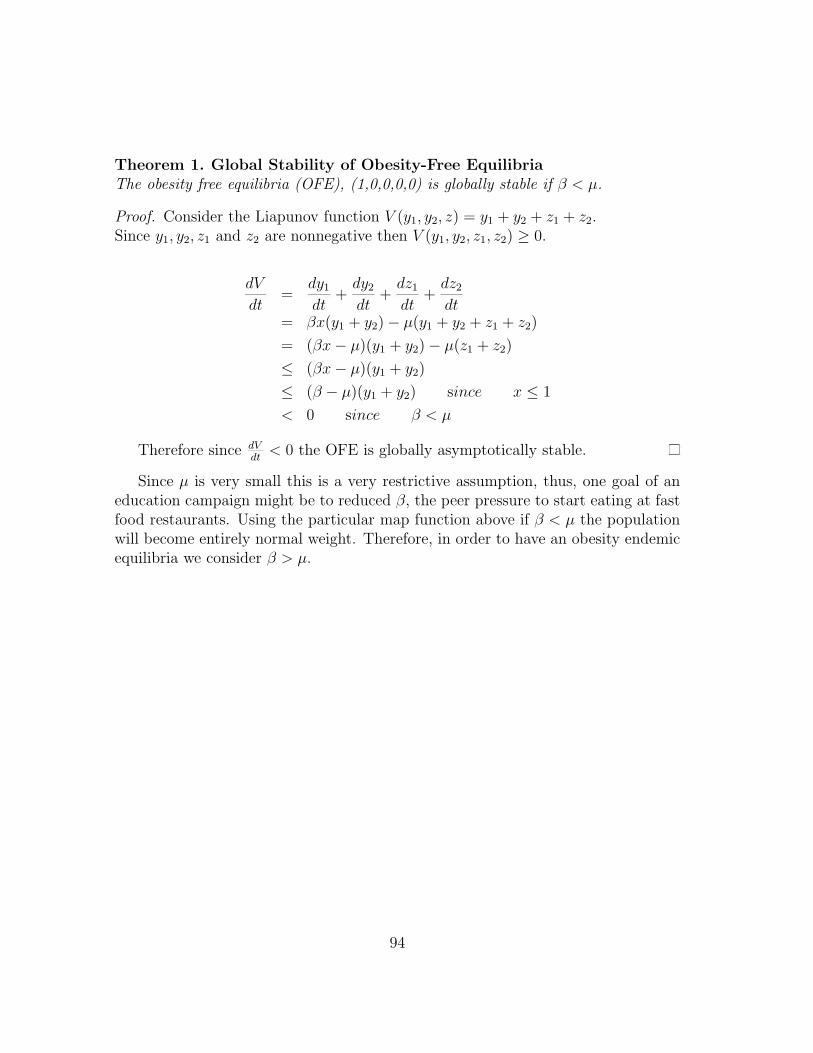
Figure 5: Obesity Model

4 Obesity Model with Nonlinear Quitting

This model focuses on the total population of individuals in the United States, whoare divided in several classes or sub-populations. The normal weight individualsN(t), are composed of the susceptible individuals who initially do not eat fast food.These individuals may start eating in fast food restaurants due to peer pressure.This peer pressure not only refers to frequent fast food eaters that invite individualsto go eat at fast food restaurants but also to factors such as time, media and indi-vidual’s socio-economic status that influenced them to go to fast food restaurants.For this project, we are assuming that eating at fast food restaurants increases theindividual’s weight. Once they start eating at fast food restaurants they becomefast food eaters and start a progression to overweight O1(t) due to large fast foodconsumption. If they continue to eat at fast food restaurants they can become obeseindividuals, O2(t). Both classes can stop eating fast food, and then move to quit-ting class, Qi(t), for i = 1, 2 for O1 and O2 respectively. The normal individuals,

91

( +( .,0, ))0. c; L+O)

fJ:;(o, +0,) 01 M, Q1 7 ~, ,;2,

rO, pi' N ( (.OO, )

a1+ L+Ol l

~v 02 ~Q, Q2 po, ,;2,

N(t), are individuals who have BMI between 18.5 and 24.5. The overweight class,O1(t), are individuals who have BMI between 24.5 and 29.9 and the obese class, areindividuals who have BMI over 29.9 [3].

Parameters:

β = Peer-pressure rate to start eating fast food (media, economic factor, etc).

µ = Mortality rate.

γ = Rate at which an overweight individual becomes an obese individual bycontinuing eating at fast food restaurants.

αi = Rate at which an individual stops eating fast food by family or health carerecommendation (quitting rate) for i = 1, 2.

α0 = Maximum quit rate due to obese individuals.

L = Obesity level at which the quit rate due to the obese individuals reaches12α0, half of its maximum.

φi =Relapse rate, for i = 1, 2.

The quitting class is consider with a non-linear term, αi + α0O2(L+O2) for i = 1, 2

that depends on the obese population, O2. This is a collective influence, like peerpressure. This section is to investigate the effects of this pressure to quit, on thesystem dynamics.

The non-linear differential equations system is:

dN

dt= µP − βN

(O1 + O2)

P− µN, (1)

dO1

dt= βN

(O1 + O2)

P+ φ1Q1 − (γ + µ)O1 −

(α1 +

α0O2

L + O2

)O1, (2)

dO2

dt= γO1 + φ2Q2 − µO2 −

(α2 +

α0O2

L + O2

)O2, (3)

dQ1

dt=

(α1 +

α0O2

L + O2

)O1 − (φ1 + µ)Q1, (4)

dQ2

dt=

(α2 +

α0O2

L + O2

)O2 − (φ2 + µ)Q2, (5)

P = N + O1 + O2 + Q1 + Q2. (6)

92

By adding all the equations the total population is constant, i.e dPdt = 0. Then

the model can be re-scale by introducing: x = NP , y1 = O1

P , y2 = O2P , z1 = Q1

P andz1 = Q1

P , with a new constant K that comes from re-scaling the nonlinear term,K = L

P . Since the total population is constant, the system can be reduced to a fourdimensional system.

dx

dt= µ− βx(y1 + y2)− µx, (7)

dy1

dt= βx(y1 + y2) + φ1z1 − (γ + µ)y1 −

(α1 +

α0y2

K + y2

)y1, (8)

dy2

dt= γy1 + φ2z2 − µy2 −

(α2 +

α0y2

K + y2

)y2, (9)

dz1

dt=

(α1 +

α0y2

K + y2

)y1 − (φ1 + µ)z1, (10)

dz2

dt=

(α2 +

α0y2

K + y2

)y2 − (φ2 + µ)z2, (11)

1 = x + y1 + y2 + z1 + z2. (12)

4.1 Obesity Free Equilibrium

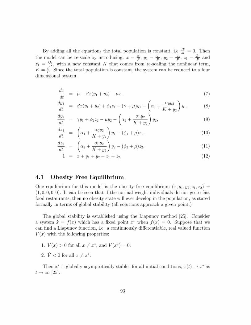
One equilibrium for this model is the obesity free equilibrium (x, y1, y2, z1, z2) =(1, 0, 0, 0, 0). It can be seen that if the normal weight individuals do not go to fastfood restaurants, then no obesity state will ever develop in the population, as statedformally in terms of global stability (all solutions approach a given point.)

The global stability is established using the Liapunov method [25]. Considera system x = f(x) which has a fixed point x∗ when f(x) = 0. Suppose that wecan find a Liapunov function, i.e. a continuously differentiable, real valued functionV (x) with the following properties:

1. V (x) > 0 for all x #= x∗, and V (x∗) = 0.

2. V < 0 for all x #= x∗.

Then x∗ is globally asymptotically stable: for all initial conditions, x(t)→ x∗ ast→∞ [25].

93

Theorem 1. Global Stability of Obesity-Free EquilibriaThe obesity free equilibria (OFE), (1,0,0,0,0) is globally stable if β < µ.

Proof. Consider the Liapunov function V (y1, y2, z) = y1 + y2 + z1 + z2.Since y1, y2, z1 and z2 are nonnegative then V (y1, y2, z1, z2) ≥ 0.

dV

dt=

dy1

dt+

dy2

dt+

dz1

dt+

dz2

dt= βx(y1 + y2)− µ(y1 + y2 + z1 + z2)

= (βx− µ)(y1 + y2)− µ(z1 + z2)

≤ (βx− µ)(y1 + y2)

≤ (β − µ)(y1 + y2) since x ≤ 1

< 0 since β < µ

Therefore since dVdt < 0 the OFE is globally asymptotically stable.

Since µ is very small this is a very restrictive assumption, thus, one goal of aneducation campaign might be to reduced β, the peer pressure to start eating at fastfood restaurants. Using the particular map function above if β < µ the populationwill become entirely normal weight. Therefore, in order to have an obesity endemicequilibria we consider β > µ.

94

D

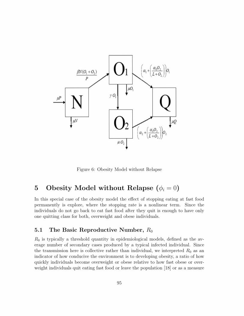
Figure 6: Obesity Model without Relapse

5 Obesity Model without Relapse (φi = 0)

In this special case of the obesity model the effect of stopping eating at fast foodpermanently is explore, where the stopping rate is a nonlinear term. Since theindividuals do not go back to eat fast food after they quit is enough to have onlyone quitting class for both, overweight and obese individuals.

5.1 The Basic Reproductive Number, R0

R0 is typically a threshold quantity in epidemiological models, defined as the av-erage number of secondary cases produced by a typical infected individual. Sincethe transmission here is collective rather than individual, we interpreted R0 as anindicator of how conducive the environment is to developing obesity, a ratio of howquickly individuals become overweight or obese relative to how fast obese or over-weight individuals quit eating fast food or leave the population [18] or as a measure

95

01 (a t( .,0, Jr' fiV(o~~ I<: LtO, JLJ,

pP N ro,

Q ~v 02 ~La:J' lP'2

f1 0)

of the number of secondary conversions to fast food use from interactions with fre-quent fast food users in a population of few fast food consumers. Since we have anonlinear term for quitting, α0 and K are not going to be present in R0 because welinearize around the OFE, no terms nonlinear in the infected class variable, obeseclass.

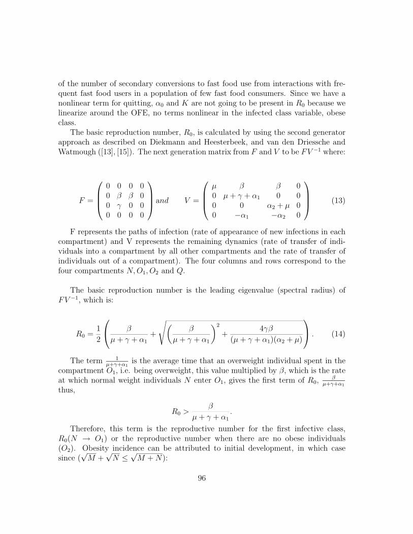
The basic reproduction number, R0, is calculated by using the second generatorapproach as described on Diekmann and Heesterbeek, and van den Driessche andWatmough ([13], [15]). The next generation matrix from F and V to be FV −1 where:

F =

0 0 0 00 β β 00 γ 0 00 0 0 0

and V =

µ β β 00 µ + γ + α1 0 00 0 α2 + µ 00 −α1 −α2 0

(13)

F represents the paths of infection (rate of appearance of new infections in eachcompartment) and V represents the remaining dynamics (rate of transfer of indi-viduals into a compartment by all other compartments and the rate of transfer ofindividuals out of a compartment). The four columns and rows correspond to thefour compartments N, O1, O2 and Q.

The basic reproduction number is the leading eigenvalue (spectral radius) ofFV −1, which is:

R0 =1

2

β

µ + γ + α1+

√(β

µ + γ + α1

)2

+4γβ

(µ + γ + α1)(α2 + µ)

. (14)

The term 1µ+γ+α1

is the average time that an overweight individual spent in thecompartment O1, i.e. being overweight, this value multiplied by β, which is the rateat which normal weight individuals N enter O1, gives the first term of R0,

βµ+γ+α1

thus,

R0 >β

µ + γ + α1.

Therefore, this term is the reproductive number for the first infective class,R0(N → O1) or the reproductive number when there are no obese individuals(O2). Obesity incidence can be attributed to initial development, in which casesince (

√M +

√N ≤ √M + N):

96

R0 <β

µ + γ + α1+

√β

µ + γ + α1

γ

α2 + µ.

The term 1α2+µ is the average time that an individual spent in the class O2, obe-

sity. Therefore, the second term is a reproductive number for the second infectiveclass, R0(N → O2), where γ is the progression rate to obesity. It involves a rad-ical because replacement of overweight individuals to obesity occurs via two stageprocess, progression: N → O1 → O2. Essentially, this type of R0 has been seen inmodels with multi stage infections ([12], [14], [18]).

Typically, if R0 < 1 the disease free equilibria of the population is stable, aswell as in this model the obesity free equilibrium is globally asymptotically stableand whenever R0 > 1 the disease free equilibria becomes unstable and the endemicequilibria is established in the population and becomes stable. Therefore, in ourcase when R0 > 1 the obese individuals persist in our population.

5.2 Endemic Equilibria

The previous section shows that if β < µ and R0 < 1 then the obesity free equilib-rium is globally asymptotically stable, meaning that neither overweight nor obesityis present in the population.To solve for the endemic equilibria where R0 > 1, theequations in system (7) (applied to this special case) are set equal to and solve forx, y1, y2 and z. Since the total population is constant, i.e. dP

dt = 0 the fact thatx + y1 + y2 + z1 + z2 can be use to simplify the system. Now define:

Ω = γ + α1 + µ (15)

∆ = α2 + µ (16)

G(y2) =α0y2

(K + y2)(17)

In this case because of the nonlinearity for quitting the number of endemic equi-libria is difficult to establish analytically, however we can prove existence of at leastan equilibrium solution.

Theorem 2. Existence of Endemic EquilibriumIf R0 > 1, then there exists at least one endemic equilibrium solution.

97

Proof. The equilibrium conditions are obtained from equations (7)-(18), and reducethe system to just one equation by expressing the equilibrium values for x, y1 and zin terms of y2:

y1 =y2

γ(∆ + G(y2)) from (9), (18)

z =y2

µ

((α1 + G(y2))(∆ + G(y2))

γ+ (α2 + G(y2))

)from (10) and (18), (19)

x =µ

βy2

γ (∆ + γ + G(y2)) + µfrom (7) and (18), (20)

and then substituting into either (8) or (11) gives an expression for y2:

0 = β

[µ(∆ + γ + G(y2))

βy2

γ (∆ + γ + G(y2)) + µ

]− (Ω + G(y2))(∆ + G(y2)). (21)

After multiplying the various terms a quartic polynomial in y2 is obtained, define:

a = µγ(β(∆ + γ)−∆Ω) (22)

b = µγ(β −∆− Ω) (23)

c = β∆Ω(∆ + γ) (24)

d = β(∆Ω + (∆ + Ω)(∆ + γ)) (25)

e = β(2∆ + Ω + γ) (26)

Therefore, the 4th degree polynomial will be:

F (y2) = Ay42 + By3

2 + Cy22 + Dy2 + E (27)

where the coefficients are functions of model parameters:

A = c + α0d + α20e + α3

0β

B = (Ke + µγ)α20 + (2dK − b)α0 + 3Kc− a

C = µγKα20 + (K2d− 2Kb)α0 + 3K2c− 3Ka

D = −K2bα0 + K3c− 3K2a

E = K3a

98

For an endemic equilibrium need the endemic solution x∗, y∗1, y∗2 and z∗ to be non-

negative and add up to 1. Looking at the equations (18)-(20), x > 0, y1 > 0, z > 0and therefore x + y1 + z > 0. Now, we know that y2 = 1 − (x + y1 + z) > 1 thisimplies that y2 > 0. Now consider F (0) and F (∞). Calculations show that

F (0) = aK3 = µγ[β(∆ + γ)−∆γ] (28)

F (∞) = α30β + α2

0e + α0d + c. (29)

From (22) notice that c > 0, d > 0 and e > 0, therefore F (∞) > 0. If F (0) < 0

which implies that(

1γ + 1

∆

)< 1

β , then by continuity of F at least one solution y∗2exists when R0 > 1 (since F (0) < 0 < F (∞)). Thus, there exists at least oneendemic equilibrium solution.

99

D

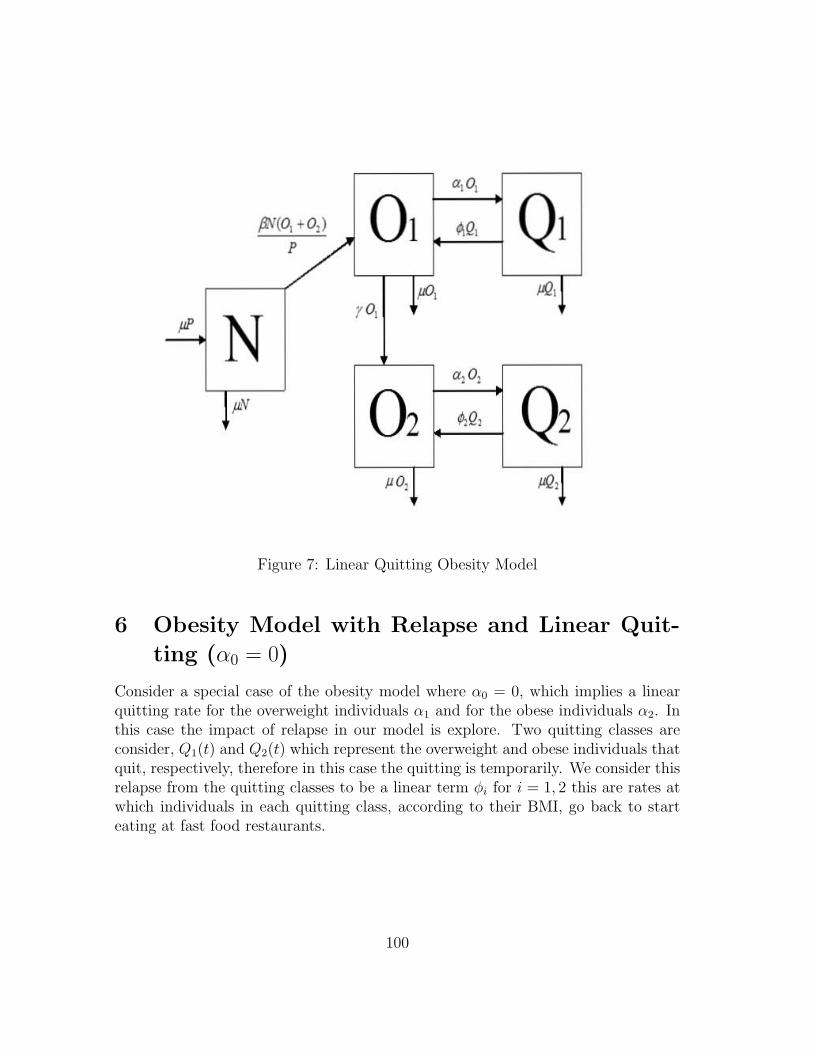
Figure 7: Linear Quitting Obesity Model

6 Obesity Model with Relapse and Linear Quit-ting (α0 = 0)

Consider a special case of the obesity model where α0 = 0, which implies a linearquitting rate for the overweight individuals α1 and for the obese individuals α2. Inthis case the impact of relapse in our model is explore. Two quitting classes areconsider, Q1(t) and Q2(t) which represent the overweight and obese individuals thatquit, respectively, therefore in this case the quitting is temporarily. We consider thisrelapse from the quitting classes to be a linear term φi for i = 1, 2 this are rates atwhich individuals in each quitting class, according to their BMI, go back to starteating at fast food restaurants.

100

a,o,

Q1 ftV'/ 01 AQ,

JiJ, pO,

pi N yo,

a2 O!

~v 02 /,Q, Q2 pO, JiJ,

6.1 The Basic Reproductive number, R0

The calculation of R0 for the relapse model was performed with the same methodas for the nonlinear quitting model. Again, F represents the paths of infection(rate of appearance of new infections in each compartment) and V represents theremaining dynamics (rate of transfer of individuals into a compartment by all othercompartments and the rate of transfer of individuals out of a compartment). Thefour columns and rows correspond to the five compartments N, O1, O2, Q1 and Q2,respectively.

The basic reproduction number is the leading eigenvalue (spectral radius) ofFV −1, which in this case tends out to be:

R0 =1

2

(β

Ω

(1 +

γ

∆

)+ p1 + p2

)+

√(β

Ω

(1 +

γ

∆

)+ p1 + p2

)2

+4p2βγ

Ω∆

(30)

where ∆ and Ω as in (15) and:

p1 =φ1Θ1

Ω, (31)

p2 =φ2Θ2

∆, (32)

Θi =αi

φi + µ. (33)

(34)

The term 1µ+γ+α1

is the average time that an overweight individual spent in thiscompartment O1, i.e. being overweight, this value multiplied by β yields the rateat which normal weight individuals N enter O1 and it multiplied by α1, gives usthe rate at which overweight individuals O1 enter Q1. Similarly, α2

µ+α2gives the rate

at which obese individuals O2 enter the class Q2, and 1φi+µ is the average time an

individual spent in the quitting class i. Thus

R0 >(β + φ1Θ1)

Ω+

φ2Θ2

∆The second term also involves a radical term similar to the model without relapse

because replacement of overweight individuals to obesity is a two stage process, pro-gression: N → O1 → O2.

101

6.2 Endemic Equilibria

The previous section shows that if β < µ and R0 < 1 then the obesity free equilib-ria is globally asymptotically stable, meaning that neither overweight nor obesity ispresent in our population. To solve for the endemic equilibria, where R0 > 1, weset each one of the equations (7)-(18) applied to this special case) equal to zero ansolve for x,y1, y2, z1 and z2.

In order to calculate the endemic equilibrium we use (15) and (31) and introducetwo new variables:

Ψ =1

γ+

1

∆− φ2Θ2, (35)

Σ =

(γ

Ω− φ1Θ1− 1

βΨ

). (36)

Therefore, the endemic equilibria for this model with relapsed and linear quittingis:

x∗ =1

βΨΣ(∆− φ2Θ2) + 1, (37)

y∗1 =µΣ

γ(∆− φ2Θ2), (38)

y∗2 = µΣ, (39)

z∗1 = µΘ1Σ(∆− φ2Θ2), (40)

z∗2 = µΘ2Σ. (41)

102

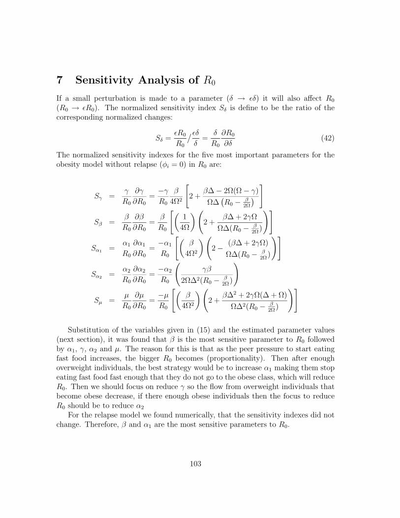
7 Sensitivity Analysis of R0

If a small perturbation is made to a parameter (δ → εδ) it will also affect R0

(R0 → εR0). The normalized sensitivity index Sδ is define to be the ratio of thecorresponding normalized changes:

Sδ =εR0

R0

/εδ

δ=

δ

R0

∂R0

∂δ(42)

The normalized sensitivity indexes for the five most important parameters for theobesity model without relapse (φi = 0) in R0 are:

Sγ =γ

R0

∂γ

∂R0=−γ

R0

β

4Ω2

[2 +

β∆− 2Ω(Ω− γ)

Ω∆(R0 − β

2Ω

) ]

Sβ =β

R0

∂β

∂R0=

β

R0

[(1

4Ω

) (2 +

β∆ + 2γΩ

Ω∆(R0 − β2Ω)

)]

Sα1 =α1

R0

∂α1

∂R0=−α1

R0

[(β

4Ω2

) (2− (β∆ + 2γΩ)

Ω∆(R0 − β2Ω)

)]

Sα2 =α2

R0

∂α2

∂R0=−α2

R0

(γβ

2Ω∆2(R0 − β2Ω)

)

Sµ =µ

R0

∂µ

∂R0=−µ

R0

[(β

4Ω2

) (2 +

β∆2 + 2γΩ(∆ + Ω)

Ω∆2(R0 − β2Ω)

)]

Substitution of the variables given in (15) and the estimated parameter values(next section), it was found that β is the most sensitive parameter to R0 followedby α1, γ, α2 and µ. The reason for this is that as the peer pressure to start eatingfast food increases, the bigger R0 becomes (proportionality). Then after enoughoverweight individuals, the best strategy would be to increase α1 making them stopeating fast food fast enough that they do not go to the obese class, which will reduceR0. Then we should focus on reduce γ so the flow from overweight individuals thatbecome obese decrease, if there enough obese individuals then the focus to reduceR0 should be to reduce α2

For the relapse model we found numerically, that the sensitivity indexes did notchange. Therefore, β and α1 are the most sensitive parameters to R0.

103

8 Parameter Estimation

In order to be able to run simulations, firs parameters must be estimated. We esti-mate the values for model parameters in order to determine model predictions. Assome of the parameters can be estimated only very roughly, our principal objectiveshall be to see how closely model behavior corresponds to pragmatic observations.

This paper focuses on the US population, which consists of approximately 300million people, of which 33% are normal weight, 34% are overweight and 30% areobese ([7], [21]). Since our model focuses on the progression of gaining weight for anormal weight individual, the initial condition for N is 99 million. In order to calcu-late the mortality rate, µ, we take into consideration the average life time of an indi-vidual which is approximately 70 years (840 months); therefore µ = 1/840 = 0.0012months −1. The time it takes an overweight individual to become obese by con-tinuing to consume fast food is approximately 7.5 months. This approximation isobtained by studying the “Super-Size Me” documentary by Morgan Spurlock, inwhich he increased his BMI value from normal weight to overweight in a period ofone month, 90 meals [24]. His case is an extreme case since all his meals were fastfood. On average, an individual consumes 12 fast food meals per month; hence ittakes approximately 7.5 month for an average individual to increase his/her weightstatus [23]. Now, the rate at which an individual progresses from the overweightcompartment to obesity is γ = 1

7.5 = 0.13 months−1.

The parameters β, α1, and α2 depend on peer-pressure; there is no accurate formof quantifying peer-pressur. In the absence of accurate data pertaining relapsed rate,we approximate φ1 and φ2 taking into consideration the fact that 33% of the USpopulation is on a diet, of which 16.5% break the diet ([5], [20]).

104

9 Numerical Simulations

Numerical solutions with respect to our model were considered in order to study thebehavior of the obesity epidemic due to fast food consumption as time progresses.A MatLab program was used to test the relevance of the peer-pressure parameters,β, α1, and α2 because from the above sensitivity analysis it was concluded that ourmodel are the most sensitive to these. In the special case were we are consideringthe possibility of relapse, the focus is given to the effect of introducing relapse ratesφ1 and φ2. In doing so, the role of peer-pressure on becoming a fast food eater andstopping eating fast food was determined.

9.1 Effect of Peer Pressure to Start Eating Fast-Food (β)

Figure (8) shows the effect of peer-pressure to start eating fast food, β. In Figure(a), β = 0.6, a peer-pressure that roughly resembles the current situation. Thischoice of β causes R0 = 3.5375 > 1, hence resulting in an obesity epidemic. Weare able to predict in a period of approximately 10 months that 35% of the normalweight individuals will become overweight. Furthermore, in roughly 18 months (1.5years), 25% of the normal weight individuals will become obese. In Figure (b), weset β = 0.09, a very low peer-pressure which maintains R0 < 1. Notice that the obe-sity epidemic is under control, keeping both the percentage of overweight and obeseindividuals to a minimum. This shows how peer-pressure has a strong influence onbecoming a fast food eater.

9.2 Effect of Peer Pressure for Overweight Individuals toStop Eating Fast-Food (α1)

Figure (9) shows the effect of peer-pressure for the overweight individuals to stopeating fast food, α1. In Figure (a), α1 is given a low value, α1 = 0.2, which results inR0 = 2.679 > 1. From the dynamics of the model, we are able to predict that in 15months (1.3 years), 22% of the normal weight individuals will become overweight.Consequently, in only 18.5 months (1.6 years), 18% of the normal weight individualswill become obese. Now, in Figure (b), the value of α1 changes to α1 = 0.95,decreasing R0 to 0.804, the obesity epidemic is under control. With this choiceof α1, the normal weight individuals will progress to the overweight compartment,however since α1 is high, these individuals will also leave the compartment at a fastrate, hence not advancing to obesity. In conclusion α1 also has a strong effect incontrolling the obesity epidemic.

105

Figure 8: Effect of Peer Pressure to Start Eating Fast Food

106

'00

00

~ 0 0

eo E-

O 0 ,

'" 0 0 D ~

'"

00

L Ro = 3 _5375 Bet a= 0 .6 alphal = 0 .1 alph a2= 0 .1 gamm a= 0 .13

35% Overwe ight (10 months)

t im e (months)

,.,

-+- Normal W eight o.erweight Obese

--B- Quit

00

L Ro =O.92ffl3 8 e l ,,= 0 _09 a lpha l = 0 1 a lpha2= 0.1 g amma= 0 _1 3

eo t ime (m onths)

,., 00

Low Pee r- P resu re

-+- Normal W eight o.e rweig hl Obese

--B- Quit

''"

''"

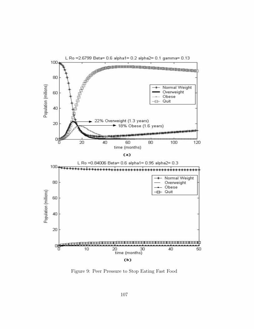
Figure 9: Peer Pressure to Stop Eating Fast Food

107

HU

00

~ 0 a eo E-o a ,

<C a a a ~

'"

'00

00

~ 0 a eo E-o a

• '" a a a ~

'"

L Ro = 2_6799 Bela= 0 .6 a lpha l = 0.2 a lpha2= 0 .1 gamma= 013

--+- Normal W eight Ove rweight Obese

--e- Quit

22% O\<e"""" ight (1 .3 years) 18% Obese (1 .6 years)

eo lime (months)

,., 00

L Ro =0 840)6 Bel a= 0 6 alphal = 0 95 alpha2= 0 3

'" CU time (months )

'"

-+- Normal Weight o.e rweight Obese

--EJ- Quit

''''

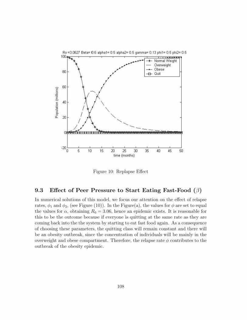
Figure 10: Replapse Effect

9.3 Effect of Peer Pressure to Start Eating Fast-Food (β)

In numerical solutions of this model, we focus our attention on the effect of relapserates, φ1 and φ2, (see Figure (10)). In the Figure(a), the values for φ are set to equalthe values for α, obtaining R0 = 3.06, hence an epidemic exists. It is reasonable forthis to be the outcome because if everyone is quitting at the same rate as they arecoming back into the the system by starting to eat fast food again. As a consequenceof choosing these parameters, the quitting class will remain constant and there willbe an obesity outbreak, since the concentration of individuals will be mainly in theoverweight and obese compartment. Therefore, the relapse rate φ contributes to theoutbreak of the obesity epidemic.

108

-0 0

i 0

~ , , • 0

"

Ro :3.ce27 Beta: 0.6 alphat : 0.5 alpha2= 0.5 gamma: 0.13 phil : 0.5 phi2= 0.5 100

ffi

.0

'"

time (months)

--+- Normal We ight o..e ...... eight

___ Obese -e- Quit

10 Conclusion

From the statistical analysis we concluded with a factor and interaction effects modelwhich explain 61.05% of the total variability in weight. The weight is statisticallysignificant different between the three age’s categories, between the five race’s cat-egories and between the three education categories, but not statistically significantdifferent between gender.

The models with support of the numerical analysis, showed that peer-pressure,β had a strong influence in becoming a fast-food eater. Furthermore, the rate atwhich individuals stop eating fast food, α1 also seemed to be effective in controllingthe obesity epidemic. It would appear that in order to reduce the current obesityrates, we should focus on lowering the peer pressure from fast food eaters. However,controlling β is difficult to achieve since β is deduced from the peer-pressure due tofrequent fast food eaters, media, social and economic status. Hence, we should gearour attention in incrementing the peer pressure to stop eating fast food, α1. This isa more realistic approach since it is easier to increment health awareness programsthat are accessible to the general public.

11 Future Work

For simplicity purposes, for this project we just considered natural mortality rates.Research indicates that obesity is also associated to other chronic mortality diseases,such as heart attacks, diabetes and certain type of cancers, therefore, for future workwe would like to add the mortality rate due to these chronic or fatal diseases, andanalyze how this new rate affect our models. Integrating this new rate would makeour total population nonconstant. Another possible extension of our model wouldbe to consider a progressive model in which a population of underweight, normaland overweight and obese individuals are considered. Another area to explore wouldbe an age structure model using the possible correlation between age and weight wefound from the statistical analysis. Finally, we would like to do a more in depthanalysis of our original model.

12 Acknowledgements

Thanks for the grants from Theoretical Division at Los Alamos National Laboratory,National Science Foundation, National Security Agency, Provost Office at Arizona

109

State University, and Sloan Foundation.

We would like to thank everybody who makes MTBI possible, special thanksto Carlos Castillo-Chavez for giving us the opportunity to do research. Thanks toLeon Arriola, Armando Arciniega, Faina Berezovsky, Gloria Crispino, ChristopherKribs-Zaleta and Mahbubur Rahman for their contribution.

References

[1] ABC news, 2004. Obsessed by Fast Food: Will Fast Food be the death ofus /? Website:http://abcnews.go.com/sections/GMA/GoodMorningAmerica/GMA0201Obsessed/with Fast food.html, 8th January.

[2] Advocate Health, 2004. Understanding calories and exercise.www.advocatehealth.com/system/info/library/articles/fitness/foodforthought/fitcalo.html.

[3] American Obesity Association, 2004. Obesity is a Chronic Disease.www.obesity.org/treatment/obesity.shtml.

[4] Bowman, S. Gortmaker, S. Ebbeling, C, Pereira M, and Ludwig, D., 2004.Effects of Fast Food Consumption on Energy Intake and Diet Quality AmongChildren in a National Household Survey. Pediatrics.113, 112-118.

[5] Calorie Control Council National Consumer Survey, 2004: Trends and statistis,2004. Website: http://www.caloriecontrol.org/trndstat.html.

[6] Castillo-Chavez, C., Feng, Z., and Huang, W., 2002. On the computation of R0

and its role on global stability. In C. Castillo-Chavez et al. (Eds.), Mathematicalapproaches for emerging and re-emerging infectious diseases, Part I, IMA Vol,125, 224-250.

[7] Census Releases 2003 U.S Population Estimates, 2003.Adults, Older people and children: latest estimates. Website:http://usgovinfo.about.com/cs/censustatistics/a/latestpopcounts.htm.

[8] CDC(Center for Disease Control), 2004. Defining overweight. Website:http://www.cdc.gov/nccdphp/dnpa/obesity/defining.htm.

[9] CDC(Center for Disease Control), 2004. Over-weight and obesity: Health consequences. Website:http://www.cdc.gov/nccdphp/dnpa/obesity/consequences.htm

110

[10] Children’s hospital Boston News, 2004. Clear Link between fast food, obesity.Website: http://web1.tch.harvard.edu/chnews/01-2004/obesity.html. January.

[11] Critser, G, 2003. Fat land: How Americans Became the Fattest People in theWorld. Houghton Mifflin Company, Boston.

[12] Diekmann, O., Dietz, K., and Heesterbeek, J. A.P (1991). The basic reproduc-tion ratio for sexually transmitted diseases, Part 1: Theoretical considerations.Mathematical Bioscienes, 107, 325-339.

[13] Diekmann, O., Heesterbeek, J.A.P., 2000. Mathematical Epidemiology of infec-tious diseases: Model building, Analysis and interpretation. Wiley, NY.

[14] Dietz, K., Heesterbeek, J. A. P., and Metz, J. P., & Tutor, D, W. (1993). Thebasic reproduction ratio for sexually transmitted diseases, Part 2: Effects ofvariable HIV-infectivity. Mathematical Biosciences, 117, 35-47.

[15] Driessche, P.V., Watmough, J., 2002. Reproduction numbers and sub-thresholdendemic equilibria for compartmental models of disease transmission. Journalof Mathematical Bioscince.20, 1-21.

[16] Department of Health and Human Services, 2002. CDC’s Role in combat-ing Obesity and the Scientific Basis for Diet and Physical Activity. Website:http://www.hhs.gov/asl/testify/t020725a.html, 25th July.

[17] Food and diet News Service, 2004. Treat yourselve better-calories. Website:http://www.foodanddiet.com/NewFiles/calorieburnchart.html.

[18] Gonzales, B. et. al. (2003) Am I too fat /? Bulimia as an epidemic. Journal ofMathematical Psychology. 47, 515-526.

[19] Mangel, M. and Clark, Colin W. (1988). Dynamic Modeling in Behavioral Ecol-ogy. Pricenton University Press, Princeton, N.J., pp. 41-81.

[20] Medline Plus, 2004. Reuters Health information. Amer-icans Abandoning Low-carb Diets-Survey. Website:http://nlm.nih.gov/medlineplus/news/fullstory 18977.html, July, 15th.

[21] National Institute of Diabetes and Digestive and Kidney Diseases of the Na-tional Institute of Health, 2004. Statistics realted to Overweight and Obesity.Website: http://www.niddk.nih.gov/health/nutrit/pubs/statobes.htm.

111

[22] Natural Strength news, 2002. Value Meals: The High Price of FastFoods.Website://www.naturalstrength.com/nutrition//detail.asp/?ArticleID=585,12th August.

[23] News Service 2think, 2004. Fast Food Nation: The Dark Side of the All-American Meal. Website: http://www.2think.org/fastfood.shtml.

[24] Recent reviews and press, 2004. SupersizeMe: A film of epic proportions. Website:http://www.supersizeme.com/home.aspx/?page=archived/06/03/04channel4.

[25] Strogatz, S.H. (1994) Nonlinear Dynamics and Chaos. Perseus Books: Mas-sachussetts.

[26] The cool nurse, 2004. Calories burned per minute for various activities. Website:htpp://www.coolnurse.com/calories.htm.

[27] World Health Organization, 2004. Facts related to chronic diseases. Website:http://www.who.int/dietphysicalactivity/publications/facts/chronic/en.

112