U.S. Navy Promotion and Retention by Race and Sex

Amos Golan, American University William Greene, New York University

Jeffrey M. Perloff, University of California, Berkeley

January, 2010

Abstract

The Navy’s promotion-retention process involves two successive decisions: The Navy decides

whether an individual is selected for promotion, and then, conditional on the Navy’s decision,

the sailor decides whether to reenlist or leave the Navy. Rates of promotion and retention depend

on individuals’ demographic and other characteristics, wars and economic conditions and factors

that the Navy policy makers can control. Using estimates of these decision-making processes, we

examine two important public policy questions: Do Navy promotion and retention rates differ

across race and sex? Can the Navy alter its promotion and other policies to better retain sailors,

or do war and civilian labor market conditions determine retention?

Key Words: promotion, retention, labor, sex, race

JEL Classification Codes: J45, J7

We thank the office of Navy Personnel Research, Studies and Technology (NPRST) for giving us permission to use the data, for replying to all of our questions and for granting us permission to publish this paper. NPRST is not responsible for our findings or conclusions.

U. S. Navy Promotion and Retention by Race and Sex

Today’s Navy wants to give all its sailors an equal chance of promotion. However, as

individuals make judgments that affect promotion decisions, it is possible that minorities and

females are treated unequally. Because the retention of sailors depends on their probability of

promotion, unequal treatment may affect which sailors stay in the Navy. Given our nation’s

military activities in Iraq and Afghanistan, the Navy’s leaders are concerned whether its policies

will enable it to retain a large proportion of its sailors. We investigate whether there are racial or

sex differences in rates of promotion in the career paths of the enlisted individuals and the degree

to which Navy policies affect the retention of sailors.

To investigate these issues, we estimate a two-step decision model using a recursive,

bivariate probit specification. First, the Navy decides whether to promote sailors based on their

current and past performance and the Navy’s current needs. Second, sailors decide whether to

remain in the Navy or leave, conditional on whether they are offered a promotion and other Navy

policies such as whether they are assigned sea duty. Whether individuals are promoted and

whether they stay depends on Navy policies, individuals’ characteristics, economic conditions in

the civilian labor market, and conditions of war or peace. To estimate the model, we use data on

virtually all Navy enlisted personnel from January 1997 through May 2008.

Our analysis of promotion and retention differs from previous studies, most of which looked

at large corporations. Two of the best-known, early studies on promotions are Wise (1975a, b).

Wise investigated the relationship between personal attributes and job performance as measured

by the rate of promotion. His basic model is a degenerate (most states are zero) first-order

Markov model. The firm decides whether to promote and the individual decides whether to stay

or leave, but these decisions are not estimated separately. The transition probability is estimated

independent of the grade level using a maximum likelihood method. Other methods that have

been used to study promotions include ordered multinomial models (e.g., Jones and Makepeace,

1996), multinomial system of censored equations (e.g., Schmidt and Witte, 1989), and random-

effects models (e.g., McDowell, et al., 1999).

Our superior data allow us to use a methodology that differs from previous studies in two

critical ways. First, we control for individuals’ abilities much more thoroughly than in earlier

2

studies. We have data on individuals’ current and past performance as well as on their aptitude

and ability, as measured by the individual’s Armed Forces Qualifying Test (AFQT) score. The

AFQT is based on the individual’s verbal and math scores, including word knowledge, paragraph

comprehension, arithmetic reasoning, and mathematics knowledge. Second, we separately

estimate equations for the firm’s (Navy’s) promotion decision and the individual’s retention

(reenlistment) decision. Many previous studies could only determine whether an individual was

both promoted and stayed with the firm.

In the next section, we describe the basic background for the promotion structure and

estimation. Then, we describe the relationship between the observed data and the promotion

probabilities. The data are discussed in Section 3. In Section 4 we discuss our main empirical

results. In Section 5 we use simulations to examine our key policy questions. We draw

conclusions in Section 6.

I. Navy Pay Grades and Promotion Rules The Navy sets many requirements on its workers. We incorporate these rules in our

estimation model.

Sailors are assigned to pay grades E1 through E9. With few exceptions, a sailor must spend a

minimum time in any given grade before promotion is possible. After a sailor has spent the

minimal time period in a grade and demonstrated a minimal level of performance, their

probability of promotion is positive until the individual has spent the maximum permitted time in

that grade without a promotion and is forced to leave the Navy.

Sailors start in pay grade E1 and are virtually automatically promoted to E2 and then E3.

Promotions to higher ranks are not guaranteed. The promotions we examine, from E4 through

E6, are based on largely objective performance evaluations.1

1 Our model can also capture demotions—moving to a lower pay grade. However, we do not discuss demotions here because there are only a handful of such cases.

Promotion to E7 also involves a

record review by a selection board. (The decision to promote someone to E8 or E9 is made by a

selection board based on a number of factors, some of which are highly subjective. We do not

examine these cases.) Consequently, we concentrate on promotions to E4 through E7, where

fewer factors are subjective.

3

To try to ensure that all sailors are treated fairly and that only the best are promoted, the

Navy uses a formal, systematic policy.2

The first component of the Final Multiple score for ranks E4 through E6 is time in service in

a pay grade. Individuals cannot take the required pre-promotion exam until they meet minimum

time in grade (TIR), which varies by pay grade.

Promotions to ranks E4 through E7 are based on an

individual’s Final Multiple score, which is a pay grade-specific value for each individual in each

promotion period. The Navy promotes sailors, within skill groups and specialties, to the next pay

grade starting with highest individual Final Multiple score until all its vacancies in that pay grade

are filled. The Final Multiple score for promotions to Grades E4 through E6 is a weighted

average of five components: time in grade, the Performance Mark Average (PMA), an

examination score, the Pass not Advance (PNA) measure, and awards. Most of the aspects of this

process are objective and leave no room for discrimination.

3

The second component is the Performance Mark Average (PMA). The PMA is based on the

individual’s fitness report, FITREP. A supervisor evaluates an individual on team work,

leadership, and other factors. Each sailor is assigned a PMA (four-point scale) score. An

individual must receive a PMA greater than or equal to 3.6 to be eligible to take the pre-

promotion exam: Early Promote (4.0 points), Must Promote (3.8), Promotable (3.6), Progressing

(3.4), and Significant Problems (2.0 points). The navy has tried to force performance mark

averages into a bell curve across all individuals, but that has seen limited success. If

discrimination or other non-objective criteria enter into the Final Multiple score, they enter

through the PMA.

The third component is the pre-promotion examination score. All eligible individuals must

take the exam. In each promotion cycle (approximately every six months depending on the pay 2 The Navy is very sensitive about possible discrimination. Navy studies of potential discrimination go back decades. For example, Golfin and Macllvaine (1995) studied the promotion opportunities of enlisted personnel with an emphasis on race and found that Whites were promoted at a higher rate than nonwhites. In response to these studies, the Navy has tried to prevent discrimination by using formal evaluations that leave relatively little room for subjective decisions. 3 The Minimal time for promotion is based on two components: Total active federal service and minimal time in pay grade. Minimum required time in pay grade is 9 months for E1 to E2 and E2 to E3, 6 months for E3 to E4, 12 months for E4 to E5, 36 months for E5 to E6 and E6 to E7.

4

grade), the Navy sets a cut score, which is the minimum exam score that an individual must

obtain to be considered for promotion. An individual who fails to pass must take another exam in

the next promotion cycle. In our empirical work, we use a variable called Pass, which is one if

the sailor takes and passes this test and the Final Multiple exceeds the cut score.

The fourth factor is the Pass Not Advance (PNA) measure. Individuals who were not

promoted the first time they were eligible because of a lack of vacant positions are awarded PNA

points that are added to the individuals’ final multiple value in the next evaluation period. Thus,

PNA points give such individuals a slight advantage over first-time test takers.

The fifth component is Awards. There are 28 different awards listed for which points can be

earned, with points varying across these awards. For example, 10 points for the Medal of Honor,

5 points for the Navy Cross, and 2 points for an Executive Letter of Commendation. Such major

awards are extremely uncommon.

Thus, the Final Multiple is a function of four objective measures and one subjective measure,

the PMA.4

Regardless of whether or not they are promoted, toward the end of a sailors’ current contract,

they must decide whether to reenlist for an additional period of service. Most sailors reenlist for

a period of four years at a time, though they may also be able to reenlist for five or six years.

Under certain circumstances, sailors can extend their service up to two years.

Some subjectivity may also enter into decision to promote a few people outside of

this system—early promotion—or to decide which sailor among several with the same Final

Multiple score is promoted. Finally, promotion from E6 to E7 involves one more stage that

introduces subjectivity. All candidates with adequate final multiples are evaluated by an

advancement board similar to the promotion boards for officers. Candidates are compared

against each other in front of a panel of raters and an iterative process is used to reach some pre-

established number of advancements.

5

All sailors are subject to the High Tenure Policy, which sets a maximum time that an

individual has in which to be promoted to the next pay grade from the current one: 10 years for

4 For promotions to Grades E4 and E5, Multiple = 0.34×Score + 0.36[(PMA×60) – 156] + 0.13[(TIR×2) + 15] + 0.13(PNA×2), where Score is the promotion test score. For Grade E6, Multiple = 0.30×Score + 0.415[(PMA×60) – 130] + 0.13[(TIR×2) + 19] + 0.11(PNA× 2). For Grade E7, Multiple = 0.60×Score + 0.40(PMA×13). 5 See Golan and Blackstone (2008) for a detailed study of Navy compensation, bonuses, and retention.

5

E4, 20 years for E5 and E6, and 24 years for E7.6

II. Model

However, we did not observe any cases in

which the High Tenure Policy was imposed. Apparently individuals who are not promoted

receive the signal and leave well before they hit their maximum time limit. Consistent with this

observation, we did not observe changes in average tenures when the rules on High Tenure

changed.

To examine the Navy’s promotion decision and an individual’s reenlistment decision, we

estimate a bivariate probit model. The first equation reflects the Navy’s decision whether to

promote based on the individual’s performance and ability as well as Navy need for sailors. The

second equation represents the individual’s decision whether to reenlist or leave the Navy

conditional on whether the individual is offered a promotion, the individual’s preferences as

capture by demographic variables, and civilian economic conditions.

Let yil be a binary variable that equals one if the individual is promoted and yi2 is a binary

variable that equals 1 if the sailor remains in the Navy. We estimate a probit system that reflects

a form of sample selection (Greene, 2008) where sailor i’s decision, yi2, is conditional on the

Navy’s decision, yi1, about sailor i:

1 1 1 1 1 1, sign( ),i i i iz x y z′= + =β ε (1)

2 2 2 1 2 2 2, sign( ),i i i i iz x y y z′= + + =β γ ε (2)

where zi1 is the latent variable related to whether the individual is promoted by the Navy, zi2, is

the latent variable for re-enlistment, and the errors are assumed to be distributed [ε1, ε2] ~

BVN(0,0,1,1,ρ), where BVN is the bivariate normal distribution and ρ is the correlation

coefficient between the two equations. This model is based on the model employed by Burnett

(1997) and developed further by Greene (1998, 2008). We estimate these probabilities and ρ

using a maximum-likelihood, bivariate probit method in the software package NLOGIT.

III. Data Our Navy data set covers virtually all enlisted sailors in all skill groups (occupations) and

pay grades (E3 through E7) from January 1997 through May 2008. We had to drop about one-

seventh of the observations due to missing data for some variables (these observations do not

change the basic moments). 6 The navy changed the High Year Tenure for E5 from 20 to 14 years in 2005.

6

A. Truncation

We start following an individual in the month in which they first receive a promotion from

January 1997 through May 2008. We then record information about that individual for each

successive 12 month period. (We experimented with shorter and longer time periods and found

that our results are not very sensitive to the choice of this interval.) Individuals are observed until

they exit or until the last period in the data set. There is no natural birth cohort, nor a period

cohort, though there is a promotion cohort: people eligible for promotion at each promotion

cycle and for each pay grade.

We consider all completed promotion decisions within our time frame, dropping data on

times to promotion that are not completed within our time frame. Consequently, the data set may

be truncated from the left—if the first promotion occurred in a year prior to the first time an

individual is observed in the data—or from the right—if the last observed promotion occurred

prior to the last period, May 2008. Because an individual’s first observation in our data set is

associated with a promotion decision, we do not use information about prior promotion decisions

in our estimation. By using this approach, we are able to measure how long it has been since the

previous promotion to a given promotion decision. Because we observe all of the enlisted

personnel at all pay grades of each skill group during the sample period and because the original

data are observed monthly, we find that dropping incomplete promotion period data does not

change the properties of our sample. Similarly, right truncation does not create a problem for us

for the same reason: We have all the completed promotion/stay decisions during the relevant

period.

B. Variables

Our dependent variables are promotion, Equation 1, and retention, Equation 2, which are

binary variables. The promotion variable indicates whether an individual is offered a promotion

by the Navy and includes those individuals who decide to leave the Navy before their promotion

materialized. The retention variable shows whether the sailor remains in the Navy, re-enlisting if

necessary.

We first discuss the demographic characteristics, Navy policies, and other explanatory

variables that are used in both the promotion and retention equations. Then we discuss those

variables that appear in only the promotion or in only the retention equation.

7

Both equations contain a sailor’s Armed Forces Qualifications Test (AFQT) percentile score.

The AFQT is given to all new recruits in the U.S. armed forces and measures their arithmetic

reasoning, mathematics knowledge, paragraph comprehension, and word knowledge (official-

asvab.com/understand_coun.htm). Because the Navy accepts only individuals with percentile

scores above 30, we observe scores from 30 to 99. Presumably the higher sailors’ AFQT value,

the more likely they are to be promoted, but the more likely they are to leave the Navy due to

greater opportunities in the civilian labor market.

Because very few sailors have completed college, we use two dummy variables to capture

education: a high-school-diploma dummy and a post-high-school-education dummy (where the

base group is sailors who did not complete high school). As extra education may indicate both

capability and self-discipline, we expect more education to increase one’s chance for promotion,

but to have an ambiguous effect on staying in the Navy.

Whether a sailor is currently on sea duty, which is sometimes voluntary, may affect

promotion positively if a supervisor believes that they gain valuable skills. If most sailors enjoy

sea duty, being assigned to sea duty may increase the probability of remaining in the Navy.

We have a separate dummy variable for each current pay grade, E4, E5, and E6. As

promotion from E3 (the base group) to E4 is relatively easy, we expect the coefficients on higher

grade dummy variables to have negative signs in the promotion equation. We expect that sailors

at higher pay grades are less likely to leave the Navy for a variety of reasons including higher

pay or a decision to make a career in the Navy or a decision to complete the twenty years of

service required for receiving Navy’s pension for life.

We use three race dummy variables: Black, Hispanic, and other, where White is the base

group.7

As our sample includes periods of peace and war, we expect rates of promotions and

retention to vary over time. We have five time variables. A September 11, 2001 dummy demarks

The equations also include a female dummy. We interact the race and female dummies

with the pay grade dummies to test for racial and sex differences in promotion and retention

across the pay grades.

7 For most of the period analyzed, the Navy’s classification scheme does not treat Hispanic as an ethnicity but as a race, where the races are mutually exclusive and exhaustive. That is, one cannot be both White and Hispanic or Black and Hispanic.

8

the shift from the “peace” period to the “war” period. A time trend, Peace Time, increases by one

each year through September, 2001, and is thereafter zero. A second time trend, War Time, is

zero before September, 2001, and zero thereafter. We also include squared terms for both the

time trends. These trends may capture various unobserved effects over time such as changes in

patriotism among the sailors and in Navy policies that are not included among the explanatory

variables such as retention bonuses and promotion and retention targets. The Navy regularly

changes the number of sailors it wants to promote and retain and its policies towards

encouraging retention. (Unlike some other branches of the armed forces, the Navy did not have

an explicit “stop-loss” policy that prevented sailors from leaving during the post-9/11 period.) In

addition, the trend variable captures the change in the ratio of the civilian wage to the Navy

wage. The relative pay of enlisted personal has increased over the last two decades. Currently,

average military pay is at about 70th percentile of the comparable civilian wage distribution

controlling for individuals’ experience and other characteristics (Congressional Budget Office,

2004, 2007; Department of Defense, 2005; Grefer 2008).

The remaining variables appear in only one of the equations. The variables in the promotion

equation that do not appear in the retention equations are related to Navy policies. To capture

possible Navy policy changes not otherwise captured by explicit variables or changes in the

attitudes of supervisors over time that might affect the probability of promotion, we interact the

race and sex dummies with the time trends.8

The AFQT was designed to be an unbiased test across race and sex (see official-

asvab.com/fairness_coun.htm). However because it tests mathematical and verbal skills that

are taught in schools, if the education of some demographic groups is inferior to that of others,

that group’s AFQT scores could be systematically lower than those of other groups. To capture

any such effect, we interact the race and sex variables with AFQT.

In addition to the dummy for current assignment to sea duty, the promotion equation includes

two measures of sea duty over a sailor’s career to date: the share of time in the Navy spent on sea

duty, and that share squared, which captures nonlinearities. Some Navy experts told us that they

expected sailors who spend a substantial portion of their career at sea would be more likely to be

8 Although we know of no reason why these interaction variables should appear in the retention equation, we experimented with including them. When we did so, all of their t-statistics were very close to zero.

9

promoted. These variables are not included in the retention equation on the grounds that the

share of one’s career already spent at sea can be viewed as “sunk costs.”

The Pass dummy captures whether an individual was eligible to take the exam and passed it.

The Pass dummy is not a perfect indicator because the Navy occasionally promotes people who

have not taken or passed the exam if they have an extraordinary need for personnel in certain

positions.9

The Navy may choose not to promote all eligible sailors depending on “demand” and

“supply” conditions. The Navy’s promotion demand variable is Vacancies, the number of open

positions to be filled by promotions at a given exam cycle for a given pay grade and a specific

occupation. The supply of sailors for promotion is the variable Takers, which is the number of

individuals, who are potentially eligible for promotion, for a period, pay grade, skill and

specialty and have taken and passed the exam. The promotion equation includes the ratio of

demand to supply, Vacancies/Takers, and that ratio squared to capture nonlinearities.

The variables in the retention equation that do not appear in the promotion equation mostly

concern family considerations and economic conditions that affect the civilian labor and housing

markets. We expect married sailors to be more likely to remain in the Navy than those who are

single. We also include the interaction of married and current sea duty. As a sailor on sea duty

receives bonus pay and may prefer (or not prefer) being at sea, the sign of this interaction is

ambiguous.

How long a sailor has been in the Navy is important because a sailor gets a full pension after

20 years of service. A sailor’s length of service is 0 to 6 years and 1 month of service in Zone A;

6 year, 2 months to 10 years, 1 month of service in Zone B; 10 years, 2 months to 15 years in

Zone C; 16 to 20 years in Zone D; and more than 20 years in Zone E (less than 1% of sailors).

We interact the zone dummies with a sailor’s length of service (months in the military). Thus,

these dummies and the interactions allow the effect of length of service to vary in the different

9 We do not include the Performance Mark Average (PMA), Pass not Advance (PNA), and the Final Multiple score because they may be a function of the race and sex dummies, which are included in the equations. In particular, the PMA (and hence the Final Multiple) is a subjective evaluation of an individual by the sailor’s supervisor, who might be partially influenced by the sailor’s race or sex. To test for possible subjectivity, we regressed PMA and the Final Multiple Score on demographic variables. Many of the coefficients on race and gender were statistically significantly different from zero.

10

zones. The closer one is to having served 20 years, Zone D, the less likely one is to leave. To

prevent sailors with relatively little time in the Navy from leaving, the Navy sometimes provides

a retention bonus to sailors in Zone A if they are performing a job that the Navy has difficulty

filling. The Navy may provide a smaller bonus for someone in Zone B, but it rarely provides a

bonus for a sailor in Zone C, and does not provide a bonus for more senior sailors.

Time in rank affects whether a sailor stays in the Navy because someone who is not

promoted quickly may choose to leave before hitting the maximum time when the sailor must

leave if not promoted. It is also important in determining whether a sailor is promoted; however,

the Pass dummy already captures this eligibility, so time in rank is not separately included in the

promotion equation.

Base pay is a sailor’s earning other than from bonuses, such as one receives while on sea

duty or to induce one to reenlist. Base pay is determined by pay grade and seniority. The only

way a sailor can receive a higher wage is by being promoted. Presumably a sailor compares this

base pay to what they could earn in the civilian market. However, this variable is highly collinear

with one’s pay grade and other factors that are already included in the equation.

To capture conditions in the civilian labor and housing markets, we supplement our Navy

data base with two macro variables that are lagged one period prior to the observation: the Gross

Domestic Product (Bureau of Economic Analyses) and the unemployment rate (Bureau of Labor

Statistics).10

We also include an estimate of each sailor’s probability of being employed in the civilian

labor market. Using data from the Bureau of Labor Statistics’ Current Population Survey (CPS) ,

the American Community Survey (ACS), and the National Longitudinal Survey (NLS) of Youth

(1979 and 1997 cohorts), we estimated an employment-unemployment probit equation for the

civilian labor market that includes individual characteristics that correspond to those in the Navy

data. In the probit, the data are weighted to reflect the over-sampling of veterans in the CPS

data.

11

10 Initially, we included many more macroeconomic variables, such as the NASDAQ closing index (Commodity Research Bureau) and the mortgage rate (Federal Reserve Bank of St. Louis), but we found that they had virtually no additional explanatory power.

11 An appendix providing a detailed definition and explanation of all the variables used in the estimation is available upon request. We considered estimating a Heckman-type model where the first equation is the employment probit, from which one obtains a Mills ratio that is used in a

11

The final variable in the retention equation is the (endogenous) promotion dummy. Sailors

decide whether to remain in the Navy after learning whether they are promoted.

IV. Empirical Results We estimated our model separately for each of the 21 skill groups: Administration, Aviation

Air Crew, Aviation ATC, Aviation Boatswain, Aviation Mechanical, Aviation Meteorologist,

Crypto Intelligence, Diver Special Warfare, Medical, Nuclear, Seabee, Submariner Electronics,

Submariner Other, Supply, Surface Combat Electronics, Surface Combat Weapons, Surface

Deck, Surface Electrical, Surface Engineering, Surface Operations, and Surface Repair.

The results are qualitatively similar across most of these skill groups. Consequently, due to

space constraints, we discuss results for only the Administration group, which is a very large

skill group with a wide range of backgrounds and abilities. Their job descriptions include

yeoman (administrative and clerical work), personnel specialist, Navy counselor (career and

recruiting), musician, mass communication specialist, and legalman (similar to a paralegal). One

motivation for choosing this specific group is that it contains a large share of minority groups

(larger than their share in the population) and that this group contains sailors with a large range

of AFQTs scores.

We start by presenting summary statistics. Then, we discuss the estimates of the recursive,

bivariate model, emphasizing race and sex issues. Next, we compare this bivariate model to a

simple probit.

A. Summary Statistics

The mean values of the relevant variables for the Administration group from 1997 to 2008

are presented in Table 1. The first column is for all sailors, the next four show the comparable

means for the four racial groups, and the last two are for males and females.

Averaged over the entire sample period, the Navy annually promotes 31% of all sailors and

of male and female sailors in any given year; 34% of Whites; and 29% of other racial groups.

Nearly all, 93%, of sailors remain in the Navy, with little variation across demographic groups.

second, wage equation. However, the resulting estimated wage for a sailor would be a linear function of the sailor’s personal characteristics, which are already included in the retention equation, and hence nearly perfectly collinear. The unemployment estimate is a highly nonlinear function of these characteristics; hence it does not pose the same collinearity problem.

12

The shares of sailors that are promoted and stay, promoted and leave, not promoted and stay, and

not promoted and leave, vary little across demographic groups.

There is relatively little variation across pay grades or zones of service among racial groups.

The fraction of sailors in Zone A (0 to 6 years and 1 month of service) ranges from 34% for

Black sailors to 37% of White, Hispanic, and other races. However, females have substantially

less experience than males, so that 45% of females are in Zone A but only 33% of males.

Females are much more likely to be in E4, 32%, than are males, 23%.

Minorities and males constitute a larger share of the Navy than of the civilian population.

The share of female sailors who are minorities—particularly Blacks—is larger than for males.

The mean AFQT intelligence or ability score is in the 55th percentile for Administration. (In

contrast, the average score is in the 89th percentile for sailors in Nuclear, which is a more

selective skill group.) Whites have a higher mean score and Blacks have a lower mean score than

do the other demographic groups.

Blacks and females are more likely to have a high school diploma than other sailors. In

Administration, 14% of those in the other races group have some post-high school education,

which is at least double the average for the other demographic groups.

Substantially more male sailors, 64%, are married than females, 47%. The share of Blacks

who are married, 56%, is 4 to 5 percentage points less than for the other racial groups.

More importantly, 39% of sailors have a Pass variable equal to one (not only did they pass

the exam but their Final Multiple exceeds the cut score so that they are eligible for promotion).

The share that Pass, ranges from 36% for Blacks, 38% for Hispanics, 41% for Whites, and 43%

for other races. Both males and females average 39%.12

The fraction of sailors on current sea duty varies relatively little across these groups, with

females being 5% more likely to be on sea duty than males. This difference is due to females

being more likely to be starting their Navy careers. Over their entire careers, males have spent

47% of their time at sea compared to 40% for females.

12 The share of sailors who take and pass the promotion exam the first time (not shown in Table 1) is 58% for males and 56% for females. This share varies slightly across races, from 60% for Whites to 55% or 56% for Blacks, Hispanics, and other races.

13

Our estimates of the probability of a sailor finding a civilian job range from 92% to 96% for

these demographic groups, with Blacks, 92%, and females, 93%, having lower probabilities than

other groups.

The means for most variables differ little between those for all sailors within a demographic

group and for just those who were promoted (not shown separately in Table 1). One exception is

that time in rank is higher for those who were promoted. The other exception is the time at sea

where those promoted have on average, four or five fewer months at sea than the overall average

for any given group.

Sailors may take into account recent promotions and whether they are on the fast track as

measured by time in rank when deciding whether to stay in the Navy. The first column of Table

2 shows that the frequency promoted falls from 79% at E3 and 38% at E4 to 23% at E5 and E6.

The fraction of sailors who remain in the Navy even though they were not recently promoted

rises with the pay grade—20% at E3, 59% at E4, 72% at E5, and 76% at E6—because

promotions are known to be less frequent at higher ranks and the pay is higher. Relatively few

sailors who are promoted leave: essentially none at E3 and only 5% at E6.

B. Bivariate Probit

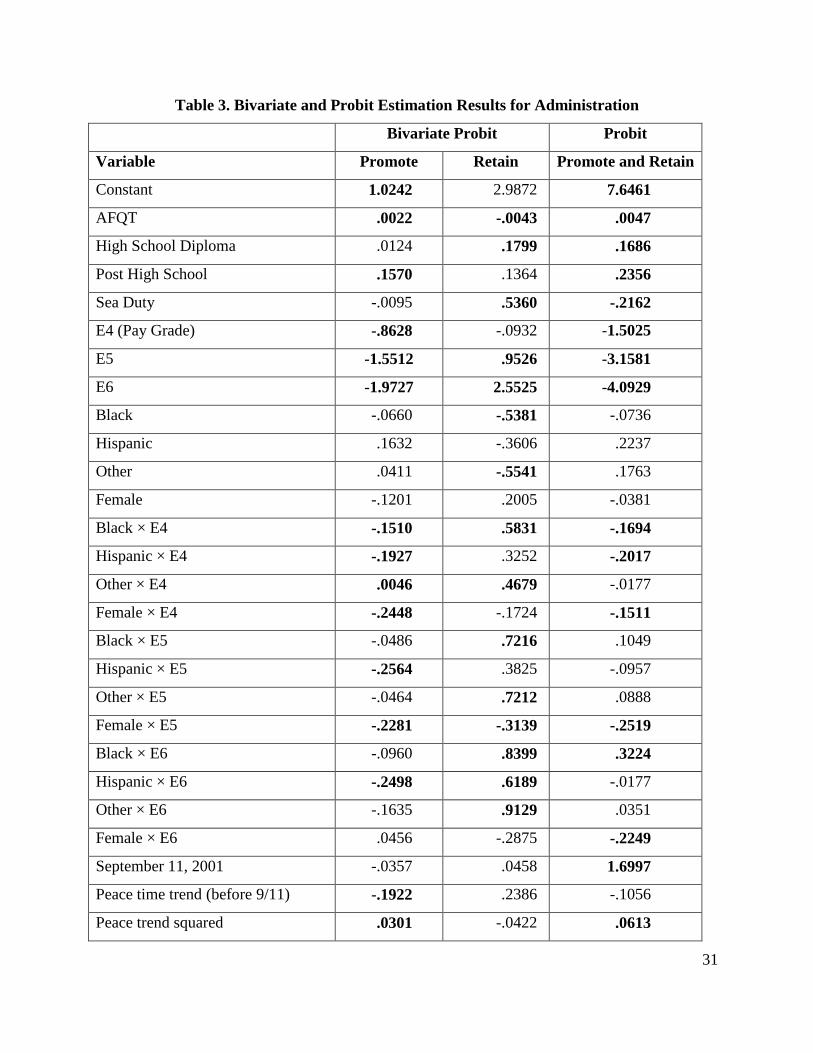
The recursive, bivariate model, Equations 1 and 2, for the Administration group fits the data

reasonably well, as the prediction table at the bottom of Table 3 shows. Most of the coefficients

have the expected signs. We concentrate on discussing those coefficients for which we can reject

the hypothesis that the coefficient is zero at the 0.05 level.

We first discuss those variables that appear in both equations. The higher a sailor’s AFQT,

the more likely the sailor is to be promoted, but the less likely to stay in the Navy. A sailor with

some post-high school education is more likely to be promoted. One with a high school diploma

is more likely to stay in the Navy. Being on current sea duty raises the likelihood of staying in

the Navy, but does not statistically significantly affect the probability of promotion. The

probability of promotion is lower in the higher pay grades, E4, E5, and E6 than in E3. Sailors in

E5 and E6 are more likely than those in E3 or E4 to remain in the Navy.

The rest of the variables that appear in both equations involve race, sex, and time trends, as

well as their interactions. Given the interactions, apart from one exception, we cannot easily

interpret their effects from the coefficients alone, so we postpone a discussion until the next

14

section, where we use simulations (and decompositions) to interpret the results. The one

exception is the stronger impact of AFQT on females.

We now turn to those variables that affect promotion but not retention. Not surprisingly, the

probability is higher if one passes the promotion exam (Pass = 1). There are two reasons why this

variable is not a perfect indicator. First, the Navy occasionally promotes individuals who do not

have sufficient time in rank or who failed the exam if the Navy’s need for sailors at higher levels

is sufficiently great. Second, promotion is also dependent on the Navy’s demand and the number

of candidates eligible for promotion. As the ratio of the number of vacancies at higher levels to

the number of sailors taking promotion exams increases, the probability of passing increases

(though at a declining rate).

Promotion depends statistically significantly on the share of a sailor’s career spent at sea

(although, as we already noted, not on whether the sailor is currently on sea duty). Initially the

effect on promotion is positive as the share increases up to 22%, but thereafter the effect is

increasingly negative as the share grows larger (and sailors have spent 45% of their careers at sea

on average).

We test whether the effect of a higher AFQT score on the probability of promotion differs

across demographic groups. The interactions are not statistically significantly different from zero

for the racial group interactions, but the coefficient on the female interaction is statistically

significantly greater than zero. Again, we postpone a discussion of the interaction effects

involving race and sex with time to the simulation section that follows.

The remaining variables affect retention but not promotion. Married sailors are more likely to

remain in the Navy. While sailors on sea duty are more likely to stay in the Navy, this positive

effect is smaller for married sailor than for others. That the effect remains positive for married

sailors may be due to the sea duty bonus pay or because the next assignment is more likely to be

shore duty.

A sailor’s history plays an important role in the decision to stay in the Navy. The longer that

a sailor has been in a given rank (that is, not promoted), the more likely that individual will

leave. The likelihood of staying in the Navy is higher for sailors with 16 to 20 years of service,

Zone D, than others, because sailors are eligible to receive a Navy pension after 20 years.

The lagged GDP has a positive effect while the Navy base pay surprisingly has a negative

one. We believe that the base pay result is due to collinearity as the base pay is largely

15

determined by one’s pay grade. As expected, the higher the overall civilian unemployment rate

or the lower a sailor’s predicted civilian employment probability, the more likely a sailor remains

in the Navy. As one would expect, a recent promotion makes it more likely that a sailor remains

in the Navy. The estimated correlation between the two equations is -0.375.

We can divide the variables into four main groups: individual attributes (AFQT, education,

race, sex and marital status), Navy-related individual attributes (pay grade, pass, base pay, zone,

length of service and related interaction variables), Navy policies (vacancies, sea duty status,

time at sea, time in rank), and the civilian labor market variables (GDP, unemployment,

individual’s employment probabilities). The interaction variables involving variables within a

group are included with that group. Because some variables appear in both equations and

because we are interested in the overall impact of each group of variables, we tested the

contribution of each of these groups on the system of promotion and retention equations. For

each one of these groups, we can reject the hypothesis that all the coefficients are simultaneously

zero at the 0.01 level. Using χ2 and other information criteria, we examined the relative

explanatory power and reduction in uncertainty of four basic groups of variables. The Navy

individual attributes contribute the most, followed in order by the individuals’ attributes, the

Navy policy variables, and the civilian labor market variables.

C. Bivariate Probit vs. Probit

Unlike in our bivariate probit model where we separately examine the decisions of the

employer (the Navy) and of the employees (sailors), most previous studies were forced to look at

the combined outcome that one was promoted and stayed with the firm. To show how estimating

this more restrictive model affects results, we estimate a probit where the dependent variable is

one when the individual is promoted and retained and zero otherwise. This probit is reported in

the last column of Table 3.

Combining the promotion and retention effects in the probit model masks offsetting effects in

the bivariate model. That is, any variable with opposite signs in the promotion and retention

equations may appear to have little or no net effect in the probit model. For example in the

bivariate probit model, having a higher AFQT score raises the probability of being promoted

(first column) and lowers the probability of staying (second column). Here, the net effect in the

probit model is positive. A sailor in pay grade E6 is less likely to be promoted than someone in

E3 and more likely to remain according to the bivariate model, but less likely to be promoted and

16

stay according to the probit model. Current sea duty does not have a statistically significant

effect on promotion, but does have a statistically significant positive effect on staying in the

bivariate model. Sea duty reduces the probability of being promoted and staying in the probit

model.

A Hispanic in E6 is less likely to be promoted but more likely to stay than a White according

to the bivariate model, whereas the Hispanic does not have a statistically significant difference to

a White in being promoted and staying according to the probit model. Similar patterns are

observed for other racial variables. Thus, the probit model does not capture patterns—

particularly those involving race—in the same way as does the bivariate model.

V. Simulations Because our bivariate probit is highly nonlinear and has many interaction variables, we

cannot infer the role of specific variables on the probabilities of promotion and retention from

the coefficients alone. To show the effects of specific variables—particularly race and sex

variables—we use two methods of simulation. In the next two subsections, we calculate the

expected probabilities over the relevant samples, such as a particular racial group, and then

average these probabilities. In the last two subsections, we simulate the effect of changing

variables on a representative sailor, where we either change a single variable at a time or a group

of related variables such as Navy policies or civilian labor market conditions.

A. Promotion and Retention by Race, Pre- and Post-9/11

Given the large number of race interactions with other variables, race can have complex

effects on the promotion and retention probabilities. Because the probability of promotion—and

to a lesser degree retention—differs substantially before and after 9/11, we report separate

simulated probabilities for the two periods. September 11, 2001 occurred roughly in the middle

of our period, dividing the peace period before 9/11 from the following war period when our

military fought in Afghanistan and Iraq.

We use our estimated model to calculate the expected probabilities for each sailor in the

relevant subsample and then average these probabilities. Our estimates reflect the substantial

change in the Navy’s promotion policies over time. For the overall sample, the probability of

promotion fell by about a fourth, going from 44.1% in the peace period to 33.8% during the war

period. Table 4 shows the changes in promotion probabilities by race and pay grade during peace

and war. The clear patterns that emerge are that promotion probabilities fall over pay grade for

17

each racial group, Whites are more likely to be promoted than are the other racial groups, and the

probabilities of promotion within any pay grade or racial group fell substantially after 9/11.

This drop in the probability of promotion is not mainly due to the war time conditions.

Rather it is the result of a long-term draw-down of the Navy starting in the 1990s together with a

sudden activation of reserves. As a consequence, there were fewer open slots available for

promotions. The end-strength (number of sailors) fell by 35% in the 1990’s and another 11%

from 2000 through 2008. The end-strength rose from 527 thousand in 1981 to a peak of 593 in

1988 and 1989. From that point, the numbers dropped: 580 in 1990, 435 in 1995, and 373 in

2000. In 2001-2002, the numbers rose slightly, hitting 385 in 2002, but then they fell again,

hitting 332 in 2008.

This reduction was achieved by reducing the number of new sailors, so the average

experience of sailors rose. As sailors with many years of service tend to remain in the Navy

because of the retirement system, the probability of retention did not change as dramatically—

from 93.3% to 92.7%—as the probability of promotion fell from peace to war time. This change

reflects the effect from a lower probability of promotion, which was partially offset by increased

average years of service, increased patriotism, and worsening civilian market conditions.

In the following, we concentrate on the probabilities of promotion and retention. However,

the retention probabilities reflect the averaging of different retention rates for sailors who were

promoted and those who were not. In Figure 1, panel a shows the probability of retention for

various pay grades by year for those sailors who were promoted. Panel b shows the retention

probability for sailors who were not promoted. From the beginning of the sample to 2001, the

retention probabilities were relatively constant for both groups of sailors. Thereafter, the

probability of retention of those sailors who were promoted fell substantially, while the

probability of those who were not promoted rose substantially. The net effect is that the share of

sailors who remained in the Navy declined only slightly during the war period.

We use simulations and decompositions to show how coefficients and characteristics affect

the promotion and retention probabilities vary across races in Table 5. We simulate average

probabilities in two ways. First, we simulate the “actual” probabilities (bold type in the table)

where we use the coefficients for a given group to calculate the probabilities for each member of

that group and average across all the member of the group. Second, we mix and match the

coefficients and characteristics other than race so that we can distinguish between the

18

contribution of coefficients, which may capture unequal evaluations for promotion by superiors,

and characteristics to the actual differences in probabilities across demographic groups. For

example, we ask how Blacks would do if they had the same coefficients as Whites (White

coefficients, Black characteristics) or if they had the same characteristics as Whites but their own

coefficients (Black coefficients, White characteristics). This type of analysis is similar to

“Oaxaca decomposition” (Oaxaca 1973), but we do it for a nonlinear model.

To save space, Table 5 presents detailed results for only the E5 pay grade. We start by

examining the pre-9/11 period (the first two columns of numbers in the table). Using each

group’s own coefficients and characteristics, we estimate that the probability of promotion for

Whites, 37.6%, was 3.9 percentage points higher than for Blacks, 33.7%. However, the

probability that a sailor stayed in the Navy is 2.7 percentage points higher for Blacks, 95.0%,

than for Whites, 92.7%. That is, Black sailors were less likely to be promoted and more likely to

stay in the Navy than White sailors. Similarly, Hispanics and other races were less likely to be

promoted and more likely to stay in the Navy than Whites (though sailors in the “other” racial

group had promotion rate similar to Whites in the pre-9/11 period).

These probability gaps reflect both differences in the coefficients between the races and

differences in each group’s non-racial characteristics. If we calculate the probabilities using the

White coefficients but the characteristics of each race, the promotion probabilities are 37.6% for

Whites, 36.5% for Blacks, 43.0% for Hispanics, and 38.2% for others. In other words, if the

Navy treated everyone equally in the sense that they had the same coefficients, then the

differences in average characteristics would make Blacks less likely to be promoted on average

than Whites, while Hispanics and other races would be more likely to be promoted than Whites.

Using the White coefficients, the average probability of retention would be lower for Whites

than for the three other racial groups given their different demographic characteristics.

If we now do the same type of analysis where we assume everyone has the average

characteristics of the White group but the coefficients for their own racial group, then we find

that the probability of promotion is 37.6% for Whites, 35.0% for Blacks, 26.6% for Hispanics,

and 36.6% for others. Thus, the difference in coefficients is most pronounced for Hispanics.

We can use these two types of analysis to loosely decompose the differences in probabilities

between groups into those due to unequal treatment as captured by the coefficients and those due

to differing characteristics. For example, the actual difference in promotion probabilities between

19

Whites and Blacks (for E5, pre – 9/11) is 3.9 percentage points (= 37.6% – 33.7%), the

difference using White coefficients and varying characteristics is only 1.1 percentage points (=

37.5% – 36.5%), while the difference using White characteristics and varying coefficients is 2.5

percentage points (= 37.5% – 35.0%). Thus, differences in the coefficients—which may capture

unequal evaluations by superiors—plays roughly twice as large a role as the difference in

characteristics in explaining the overall difference in promotion probabilities between Whites

and Blacks.

The comparable percentage point differentials between Whites and Hispanics are 5.7

percentage points (overall), –5.4 percentage points (varying characteristics), and 11.1 percentage

points (varying coefficients). One possible interpretation of these results is that Hispanics’

superior average characteristics cut half the difference in promotion probabilities due to unequal

treatment by superiors.

Has the situation changed as the Navy has shifted from peace to war? The actual gap in

promotion probabilities between Whites and Blacks went from 3.9 percentage points before 9/11

to 6.2 percentage points after 9/11, from 5.7 percentage points to 8.7 percentage points for

Hispanics, and from 4.3 percentage points to 4.5 percentage points for others. These increased

promotion gaps are even more striking given that the probability of promotion fell for all groups.

If we hold characteristics fixed using the average for the White group and vary coefficients,

the difference in promotion probabilities were 2.6 percentage points for Blacks, 11.0 percentage

points for Hispanics, and 1.0 for others before 9/11. The corresponding differentials during the

war years are 2.3, 5.3, and 0.6. Thus, these differentials that may be attributed to Navy actions

have shrunk over time.

It follows that the increase in the actual differential must be due to changes in the relative

characteristics of the various groups. If we use the White coefficients and vary characteristics

across racial groups, the difference in promotion probabilities were 1.2 percentage points for

Blacks, –5.4 percentage points for Hispanics, and –0.6 for others during peace time. The

corresponding differentials during war are 4.3, 4.7, and 4.1. The major reason why the actual

differentials between Whites and other groups have increased over time is due to relative

changes in the characteristics of nonwhite groups. These changes in characteristics are so large

that they swamp the coefficient effects that go in the other direction.

20

The changes in retention probabilities over time are much smaller than for promotion

probabilities. The probability of staying in the Navy fell by 0.9 percentage points for Whites, 0.7

for Blacks, and 1.0 for Hispanics and others.

Gaps in the promotion probabilities between the races are qualitatively similar between pay

grades, but the size of the gaps vary. During the war period, Whites are 8.5 percentage points

more likely to be promoted than Blacks in E4, 6.2 percentage points more likely at E5, and 8.2

percentage points more likely at E6.

B. Promotion and Retention by Sex, Pre- and Post-9/11

Males are substantially more likely to be promoted than females in the lower pay grades (up

to E5). Females are more likely than males to stay in the Navy at E4, but are less likely at E5 and

E6. The overall probabilities of promotion and retention fell for both sexes from the peace to the

war periods.

Again, we decompose the differences in the actual probabilities into those based on

differences in coefficients and those based on differences in characteristics other than sex in

Table 6. For E5, the actual differential between men and women was 2.0 (= 36.0% – 34.0%)

percentage points during the peace period. Using coefficients for males and varying

characteristics, the differential was 2.5 percentage points. Using characteristics of males and

varying the coefficients, the differential was –1.0. One interpretation is that the Navy slightly

favored females, but differences in characteristics between males and females caused men to be

more likely to be promoted.

The corresponding differentials during the war period are 8.7 percentage points (actual), 3.8

percentage points (varying characteristics), and 5.3 percentage points (varying coefficients).

Thus, the actual gap at E5 between men and women increased because the Navy apparently went

from favoring women to favoring men and the average characteristics of women became less

attractive relative to those of men.

We observe a qualitatively similar pattern for E4, but a strikingly different one for E6. The

E6 differentials were –3.2 percentage points (actual), –2.4 (varying characteristics), and –0.7

(varying coefficients) during peace; and are –0.8, 1.4, and –2.2 during war. Thus, it appears that

the Navy favored E6 women during peace and even more so during war. However, women had

relatively more attractive characteristics during peace than during war. The net effect is that E6

21

women were much more likely than men to be promoted during peace but only slightly more

likely during war.

For E5, men were 0.9 percentage point more likely to stay in the Navy than women based on

the actual probabilities during peace. Using men’s coefficients and varying the characteristics

results in the same differential, 0.9. Using male characteristics, and varying the coefficients, the

differential is eliminated. Corresponding differentials during war are 1.4 percentage points

(actual), 1.2 percentage points (varying characteristics), and 0.1 percentage points (varying

coefficients). Thus, the pattern of differentials does not vary much over time.

C. Effects of Specific Variables on Promotion and Retention

To learn how specific variables affect the probabilities, we conduct simulation experiments

based on a typical sailor or base case in the Administration skill group. The characteristics of our

typical sailor are the overall sample means or the mode case. The typical sailor is married, a high

school graduate, in pay grade E4, currently is on shore duty, has an AFQT of 56, 105.9 months

of service, 31.6 months of time in rank, spent 42.7% of his or her Navy career at sea, is eligible

for promotion, has a pass rate on the exam of 37.1%, has a base pay of $26,746, and has an

estimated probability of civilian employment of 94.5%. In 1998, the base period, the ratio of

Vacancies to Takers was 0.32, the civilian unemployment rate for 4.9%, and the annual GDP

was $9,520 billion.

The columns in Table 7 show how the probabilities of promotion vary across racial and sex

groups for our typical sailor. The rows in Table 7 show how the probability of promotion

changes relative to the base case as we change one variable at a time. The first row shows the

probabilities of promotion for the base characteristics. The number in the first column of the first

row, 60.7% is the probability that a White male was promoted. The second column of the first

row shows that a White female’s probability of promotion was only 49.5%, or 11.2 percentage

points less than for a White male. The third column shows that a Black male’s probability was

only 53.6%, or 7.1 percentage points less than for a White male.

Moving down the rows, we show how the promotion probability changes for a given race/sex

combination as we change one variable at a time. The first row, the base case, of the first

column, White male, shows that with the mean AFQT score, the sailor’s probability of

promotion is 60.7%. The second row shows that raising the sailor’s AFQT score to 80 increases

his probability of being promoted by 2.2 percentage points to 62.9%. The other columns show

22

that this increase in AFQT score raises each race/sex group’s probability of promotion by 2.2 to

2.4 percentage points. Similarly, the third row shows that lowering the AFQT to 35 reduces the

promotion probabilities for the various demographic groups, but by smaller absolute amounts

than raising it. As was discussed earlier, due to the additional AFQT impact for females, in all

cases the increase in the rate of promotion due to an increase in AFQT is larger for females.

Having some post high school education raises the probability of promotion by between 5.4

to 6.1 percentage points. As we are controlling for intelligence as measured by the AFQT,

presumably a sailor with post high school education is rewarded because of some extra

knowledge or better discipline that is associated with the extra education.

Being currently on sea duty lowers the probability of promotion by 0.2 percentage point for a

White male. As we noted above, the share of time spent on sea duty has a nonlinear effect, rising

up to 22%, and then falling. Increasing the share of time during one’s Navy career spent at sea

from the average of 42.7% to 64.1% (≈ 1.5 × 42.7%) decreases one’s probability of promotion

substantially. A White male’s probability falls from 60.7% to 36.7%, a White female’s

probability drops from 49.5% to 28.7%.

As we have already noted, the probability of promotion fell substantially over the last half of

the sample period. For a White male, the probability was 60.7% in 1988, 43.9% in 2002, and

only 9.5% in 2007. For a Black female, the probability dropped from 42.4%, to 30.9%, to 4.9%.

Similarly, the probability of promotion is lower at higher ranks. A typical White male’s

probability is 60.7% at E4, but only 34.1% at E5.

Retention probabilities also vary with characteristics to a lesser degree. A White male with

the base characteristics had a probability of being promoted and retained in the Navy of 60.5%

and a probability of not being promoted but retained of 39.0%, so his probability of remaining in

the Navy was 99.5% (= 60.5% + 39.0%). The corresponding probabilities are 49.4%, 50.0%, and

99.4% for a White female and 53.5%, 46.2%, and 99.7% for a Black male. Thus compared to a

White male, a White female and a Black male are less like to be promoted and stay and more

likely to not be promoted and stay, so that the overall probability of staying is virtually the same

as for the White male. Because sailors with all race and sex groups are almost certain to stay,

these differences in the joint probabilities reflect primarily the differences in the probabilities of

being promoted.

23

When conditions are bad in the civilian labor market, sailors are more likely to remain in the

Navy. If the civilian unemployment rate increases from 4.9% to 6.3%, the probability that a

White male remains rises by 0.2 percentage points if promoted and by 0.3 percentage points if

not promoted. If that sailor’s estimated individual probability of finding civilian employment

falls from 94.5% to 75%, a White male’s probability of remaining in the Navy rises by 0.1

percentage point if promoted and by 0.2 percentage point if not promoted. These quantitative

effects are small because virtually all E4 sailors remained in the Navy under any circumstances

in 1998. The quantitative effects are larger for more recent years, thought the qualitative effects

are the same.

D. Changes over Time Due to Navy Policies and Civilian Labor Market Conditions

The probabilities of being promoted and staying in the Navy changed substantially over time.

Table 8 compares various demographic groups’ probabilities in two years. The first year, 1998,

was one of peace in which economic conditions were excellent and the Navy was near its peak

size. The second year, 2006, is a war year near the end of our sample when economic conditions

were poor and the Navy had shrunk substantially.

In contrast to the last simulation experiment where we freeze all but one explanatory

variable, we now use the actual Navy policy and economic condition variables for each of our

two years for our typical E4 sailor. Across race and sex groups, the promotion probability

dropped substantially from between 40% and 59% in 1998 to between 5% and 10% in 2006. The

probability of remaining in the Navy increased moderately from between 76% and 88% in 1998

to between 83% and 92% in 2006. A key reason why the retention probabilities didn’t plummet

despite the lower probability of promotion is that civilian economic conditions were substantially

worse in 2006 than in 1998.

We can decompose the shifts over time due to three groups of variables: Navy policy

variables (pass rate, vacancies/takers, time in rank, current sea duty status, share of time on sea

duty, and length of service in zone A), civilian economic conditions (unemployment rate, the

individual’s employment probability, and GDP), and time trends including the 9/11 dummy. In

these experiments, we hold the E4 sailor’s base personal characteristics (AFQT, marriage status,

and so forth) constant and then use various combinations of Navy policy variables, civilian

economic condition variables, and time trends for 1998 or 2006.

24

Table 9 shows our eight hypothetical experiments: each of three groups of variables can take

on 1998 or 2006 values. The first row shows what happens if all the variables are set at their

2006 levels: a White male sailor’s probability of promotion is only 9.9%, his unconditional

probability of staying in the Navy is 88.3%, the conditional probability of staying if promoted is

92.4%, and the conditional probability if not promoted is 87.8%. Thus, having been promoted

raised his conditional probability of staying in the Navy by 4.6 percentage points (= 92.4% –

87.8%). These simulations are examining hypothetical situations and hence do not correspond to

actual observed patterns.

The second row shows the corresponding probabilities if all three groups of variables are set

at their 1998 levels: 58.7%, 84.5%, 87.9%, and 79.6%. At 1998 levels, the sailor was more than

5 times as likely to be promoted, but his unconditional and conditional probabilities of remaining

in the Navy were lower than in 2006.

We can assess the relative contributions of each group of variables on the probability of

promotion by changing one group of variables at a time and comparing the results to those in

row 1. In row 3 where the Navy policies are at their 1998 levels and the other variables are at

their 2006 levels, the probability of promotion is 2 percentage points higher than when Navy

policies are at their 2006 level (row 1). Changing only the civilian labor conditions (row 4) has

no effect on the promotion probability because they do not depend on civilian labor conditions. If

we keep the Navy policy variables and labor market conditions at their 2006 level but set the

time trends to their 1998 level (row 5), the promotion probability rises by more than 5-fold to

54.4%. The time trend variables capture the size-of-the-Navy effect, which is not included in the

Navy policy variables. The Navy was at its peak size in 1998, and as a consequence, promotion

rates were high. If we change the Navy policies and the time trends to their 1998 level (row 7),

the probability of promotion is 58.7%, or only 4.3 percentage points higher than from changing

the time trends alone. Thus, changing the Navy policies other than the size of the Navy back to

the “good old days” would have had a relatively small effect on promotion and retention

probabilities.

We can similarly conduct hypothetical simulation experiments concerning the effects of the

groups of variables on retention probabilities, where civilian labor market conditions play a

prominent role. If civilian labor market conditions were at their excellent 1998 levels while the

Navy policies and time trends were at their 2006 levels (row 4), the unconditional retention

25

probability would have been 5.3% instead of the observed 88.3%. That is, given the very low

promotion rates in 2006, if the sailor had decent opportunities in the civilian labor market, he

would have almost certainly have left.

Changing only the time trends to the 1998 level (row 5) would have increased the retention

probability from 88.3% to 99.9%. Thus, any increased retention due to patriotism in the post-

9/11 era was more than offset by other changes over time including being in wartime conditions.

If both labor market conditions and time trends were at their 1998 level (last row), the

probability would have been 83.3%, only slightly lower than the observed 2006 probability of

88.3%. Thus, these simulation experiments indicate that Navy policies contribute much less to

keeping sailors in the Navy than did civilian labor market conditions.

VI. Conclusions Our promotion and retention study is the first to simultaneously examine the separate

decisions of the employer and the employees while controlling for employees’ abilities using an

intelligence or ability test score. This model allows us to examine two important policy

questions: Does the Navy treat various demographic groups unequally? Do the Navy’s policies

have an important effect on retention?

We have very clear-cut results concerning race. Despite the Navy’s elaborate controls to

ensure fairness, the probability of promotion varies statistically and significantly across races and

by sex. Blacks, Hispanics, and other races were less likely to be promoted and more likely to stay

in the Navy than Whites. Though we provide here detailed analysis of only one basic skill

group, our results are robust and qualitatively similar across all of the skill groups.

The annual probabilities of promotion and retention could differ across racial and sex for

three reasons. First, demographic groups could be treated differently by the Navy in the sense

that people with the same characteristics but who differ in terms of race or sex have different

probabilities (that is, the coefficients on individuals’ characteristics are the same across

demographic groups). Second, these groups could have different mixes of observed

characteristics such as education and experience. Third, there could be differences in unobserved

characteristics across the demographic groups.

Differences in coefficients (the first hypothesis) play roughly twice as large a role as the

difference in observed characteristics (the second hypothesis) in explaining the overall difference

in promotion probabilities between Whites and other races. The difference in coefficients is most

26

pronounced for Hispanics. We cannot explicitly examine the third hypothesis. However,

because our bivariate probit analysis includes an objective ability measure, the AFQT score, as

well as a large number of other observed characteristics, it is relatively unlikely that racial and

sex differences in promotion rates reflect unmeasured ability differences across demographic

groups13

The gap in promotion probabilities between Whites and other races increased moderately

from before to after 9/11. The part of the differentials due to Navy actions (as captured by the

coefficients) has shrunk over time, so that the increase in the actual differential is due to changes

in the relative characteristics of the various groups.

.

The results concerning the treatment of the sexes vary across pay grades. Males are

substantially more likely to be promoted than females in pay grades up to E5. During the war

years, the actual gap at E4 and E5 between men and women increased both because of changes

in the sex coefficients and because the average characteristics of women became less attractive

relative to the Navy than those of men. In contrast, E6 women did better than men during peace

and even more so during war. However, these women had relatively more attractive

characteristics during peace years than during war years. The net effect is that E6 women were

much more likely than men to be promoted during peace but only slightly more likely during

war. Females are more likely than males to stay in the Navy at E4, but are less likely at E5 and

E6.

Individual characteristics matter, but no single characteristic other than race or sex plays a

dominant role. For example, intelligence or ability as measured by the AFQT score plays a

relatively small role in determining promotions. Raising the typical E4 sailor’s score from the

55th percentile to the 80th increases the promotion probability 2.2 percentage points.

Higher rates of promotion slightly increase the odds that a sailor remains in the Navy. Since

the late 1990’s, the Navy has been shrinking, despite war time conditions during much of this

period. Apparently as a consequence, the rate of promotion has plummeted: For a typical White

male E4 sailor, the probability of promotion fell from 58.7% in 1998 to 9.9% in 2006.

13 We note that AFQT does not capture all of the unobserved abilities. For example, verbal fluency, writing ability, sociability, etc., which are all related to promotions in civilian jobs, are not captured by AFQT and education (at the HS level).

27

Nonetheless, retention rates have remained relatively high in recent years because of the

increasing lack of opportunities—particularly for minorities—in the civilian labor market and the

relative increase in the Navy pay relative to civilian wages

When conditions are bad in the civilian labor market, sailors are more likely to remain in the

Navy. For most of the time period, this effect was quantitatively small because almost everyone

remained in the Navy. Now, these conditions may matter more. Our model does a good job of

predicting the actual observed retention rate in 2006 of 88.3% based on actual Navy policies and

the poor labor market conditions in that year. However, if we conduct the hypothetical

experiment where we change the civilian labor market conditions to their excellent 1998 levels

but keep all other 2006 conditions (such as the wars) including Navy policies the retention

probability would have fallen significantly. That is, given the very low promotion rates in 2006,

if the sailors had good opportunities in the civilian labor market, most of them would have left.

These simulations show that Navy policies (other than the size of the Navy) contribute much less

to keeping sailors in the Navy than do civilian labor market conditions. Consequently, if the

Navy remains small and has a low probability of promotion, it faces the risk that when civilian

economic conditions improve, the Navy could lose many of its enlisted sailors upon the

expiration of their tours of duty. To avoid that outcome, the Navy may have to raise the

promotion rate, pay substantial re-enlistment bonuses, continue to increase the Navy’s relative

wage, or take other financially costly actions.

28

References

Golan, Amos, and Tanja F. Blackstone. 2008. Models of Compensation: Policy Analyses and

Unemployment Effects, Navy Personnel Research, Studies, and Technology Division,

Bureau of Navy Personnel, NPRST-TR-08-03.

Burnett, Nancy J. 1997. “Gender Economics Courses in Liberal Arts Colleges,” Journal of

Economic Education, 28: 369-377.

Congressional Budget Office. 2004. “Educational Attainment and Compensation of Enlisted

Personnel.”

Congressional Budget Office. 2007. “Evaluating Military Compensation,” Congressional Budget

Office Report Released June 29.

Department of Defense. 2005. Military Compensation Background Papers.

Greene, William H. 2008. Econometric Analysis, 6th Edition, New York: Prentice Hall.

Greene, William H. 1998. “Gender Economics Courses in Liberal Arts Colleges: Further

Results,” Journal of Economic Education, 29: 291-300.

Gofin, Peggy A., with Martha E. Macllvaine. 1995. Mid-Career Enlisted Promotion; Effect of

Service and Personal Characteristics, Center for Naval Analysis, CRM 95-120.

Grefer, James. 2008. “Comparing Military and Civilian Total Compensation,” Center for Naval

Analysis.

Jones, David R., and Gerald H. Makepeace. 1996. “Equal Worth, Equal Opportunities: Pay and

Promotion in an Internal Labor Market,” Economic Journal, 106, 401-409.

McDowell, John M., Larry D. Singell, Jr., and James P. Ziliak. 1999. “Cracks in the Glass

Ceiling: Gender and Promotion in Economics,” American Economic Review (Papers and

Proceedings), 89: 392-396.

Oaxaca, Ronald. 1973. “Male-Female Wage Differentials in Urban Labor Markets,”

International Economic Review, 14: 693-808

Schmidt, Peter, and A. D. Witte. 1989. “Predicting Criminal Recidivism Using ‘Split Population’

Survival Time Models,” Journal of Econometrics, 40: 141-159.

Wise, David A. 1975a. “Personal Attributes, Job Performance, and Probability of Promotion,”

Econometrica, 43: 913-931.

Wise, David A. 1975b. “Academic Achievement and Job Performance,” American Economic

Review, 65: 350-366.

29

Table 1. Means (%) for the Administration Skill Group

All White Black Hispanic Other Male Female Promoted 31 34 29 29 29 31 31 Stay in the Navy 93 91 94 94 94 93 92 Promoted/Stay 26 27 25 26 25 26 26 Promoted/Leave 5 7 4 3 4 5 5 Not Promoted/Stay 67 64 69 69 69 67 66 Not Promoted/Leave 2 2 2 3 2 2 3 E4, pay grade 26 23 27 27 25 23 32 E5 36 35 36 36 34 36 34 E6 31 34 30 29 34 28 25 Zone A 37 37 34 37 37 33 45 Zone B 26 24 27 27 27 27 25 Zone C 23 24 24 23 25 26 18 Zone D 13 15 13 12 11 14 12 Black 37 0 100 0 0 34 44 Hispanic 11 0 0 100 0 11 12 Other 9 0 0 0 100 9 8 Female 30 25 35 31 28 0 100 AFQT 55 63 47 53 54 56 52 High School Diploma 88 87 92 86 80 87 91 Post High School 7 7 5 6 14 7 6 Married 59 61 56 60 61 64 47 Pass 39 41 36 38 43 39 39 Sea Duty 51 50 52 49 47 49 54 Share Sea Duty 45 44 44 49 48 47 40 Probability of civilian employment 94 96 92 95 96 95 93 Vacancies/Takers (× 100) 32 33 31 30 35 32 32 Time in Rank (months) 30 31 29 26 29 31 27

Notes: All means are percentages except for time in rank (months) and Vacancies/Takers, which is multiplied by 100. AFQT is the Department of Defense test of ability. Zone A: 0 to 6 years and 1 month of service. Zone B: 6 year, 2 months to 10 years, 1 month. Zone C: 10 years, 2 months to 15 years. Zone D: 16 to 20 years. Zone E (not reported): more than 20 years. Averages are based on 53,556 observations.

30

Table 2. Frequencies (%) by Pay Grade

Promoted

Stay

Not Promoted,

Stay

Promoted,

Stay

Not Promoted,

Leave

Promoted,

Leave

E3 79 99 20 79 1 ~0

E4 38 96 59 37 3 1

E5 23 93 75 18 2 5

E6 23 89 76 13 1 1

Note: Due to rounding, the last four elements of each row may not add to 100.

31

Table 3. Bivariate and Probit Estimation Results for Administration

Bivariate Probit Probit

Variable Promote Retain Promote and Retain

Constant 1.0242 2.9872 7.6461

AFQT .0022 -.0043 .0047

High School Diploma .0124 .1799 .1686

Post High School .1570 .1364 .2356

Sea Duty -.0095 .5360 -.2162

E4 (Pay Grade) -.8628 -.0932 -1.5025

E5 -1.5512 .9526 -3.1581

E6 -1.9727 2.5525 -4.0929

Black -.0660 -.5381 -.0736

Hispanic .1632 -.3606 .2237

Other .0411 -.5541 .1763

Female -.1201 .2005 -.0381

Black × E4 -.1510 .5831 -.1694

Hispanic × E4 -.1927 .3252 -.2017

Other × E4 .0046 .4679 -.0177

Female × E4 -.2448 -.1724 -.1511

Black × E5 -.0486 .7216 .1049

Hispanic × E5 -.2564 .3825 -.0957

Other × E5 -.0464 .7212 .0888

Female × E5 -.2281 -.3139 -.2519

Black × E6 -.0960 .8399 .3224

Hispanic × E6 -.2498 .6189 -.0177

Other × E6 -.1635 .9129 .0351

Female × E6 .0456 -.2875 -.2249

September 11, 2001 -.0357 .0458 1.6997

Peace time trend (before 9/11) -.1922 .2386 -.1056

Peace trend squared .0301 -.0422 .0613

32

War time trend (after 9/11) -.4823 -.6293 -.4028

War trend squared .0313 .0515 .0674

Pass .7354 1.0979

Vacancies/Takers .3145 1.2254

Vacancies/Takers Squared -.0129 -1.3283

Share Sea Duty (fraction) .6779 .3844

Share Sea Duty Squared -1.5162 -.3392

Black × AFQT -.0000 -.0029

Hispanic × AFQT -.0018 -.0021

Other × AFQT -.0003 -.0019

Female × AFQT .0027 -.2249

Black × Peace trend .0919 .0829

Black × Peace trend squared -.0182 -.0182

Black × War trend .1168 .0999

Black × War trend squared -.0184 -.0161

Hispanic × Peace trend .0228 .0474

Hispanic × Peace trend squared .0014 -.0118

Hispanic × War trend .0471 -.0074

Hispanic × War trend squared -.0036 -.0014

Other × Peace trend .0168 .0117

Other × Peace trend squared -.0055 -.0075

Other × War trend .0176 .0039

Other × War trend squared -.0026 -.0058

Female × Peace trend .0624 .0342

Female × Peace trend squared -.0123 -.0007

Female × War trend -.0643 .0452

Female × War trend squared .0199 .0003

Married .2559 .1433

Married × Sea Duty -.1675 .0327

Zone A -5.2517 1.8162

33

Zone B -5.1929 2.4689

Zone C -3.8933 3.5990

Zone D 6.3486 8.5744

Length of Service × Zone A .0363 .0105

Length of Service × Zone B .0364 .0001

Length of Service × Zone C .0251 -.0075

Length of Service × Zone D -.0289 -.0346

Time in Rank .0109 .0234

Base pay -.4902 .0776

GDP 1.1552 -1.0627

Unemployment. Rate (%) .6669 -.1064

Probability of civilian employment

(fraction) -1.8010 -2.3376

Promoted .9120

Rho -.3575

Notes: A bold coefficient indicates that the p-value is less than 0.05. There are 53,556

observations. The log-likelihood statistic is -31,148 for the bivariate probit and -18,598 for the

probit. The probit McFadden pseudo R2 is 0.39.

The Bivariate Probit Prediction Table The Probit Prediction Table

Actual over (Fitted values in parentheses) (1 = Promoted and Retained)

Retained

Promoted

Actual

Value

Predicted Value

0 1 Total 0 1 Total

0 1,084

(2,126)

2,700

(353)

3,784

(2,479) 0

36,843

(68.8%)

2,759

(5.2%)

39,602

(73.9%)

1 35,818

(41,149)

13,954

(9,928)

49,772

(51,077) 1

5,374

(10.0%)

8,580

(16.0%)

13,954

(26.1%)

Total 36,902

(43,275)

16,654

(10,281)

53,556

(53,556) Total

42,217

(78.8%)

11,339

(21.2%)

53,556

(100%)

34

Table 4. Promotion Probabilities by Pay Grade, Race, and Sex

White Black Hispanic Other Male Female

Pre-9/11

E4 56.7 47.9 51.1 55.3 54.0 49.7

E5 37.6 33.7 31.9 37.3 36.0 34.0

E6 40.6 33.6 34.9 35.7 36.4 39.6

Post-9/11

E4 45.9 37.4 37.0 40.0 43.1 37.1

E5 29.4 23.2 20.7 24.9 28.2 19.5

E6 29.9 21.6 20.2 24.8 25.5 26.3

35

Table 5. Predicted Probabilities (%) by Race for E5

Pre-9/11 Post-9/11

Coefficients

Characteristic

s Promotion Retention Promotion Retention

White White 37.6 92.7 29.4 91.8

White Black 36.5 95.0 25.1 94.4

White Hispanic 43.0 95.2 24.7 93.9

White Other 38.2 96.1 25.3 95.1

Black White 35.0 92.6 27.1 91.7

Black Black 33.7 95.0 23.2 94.3

Black Hispanic 34.3 94.9 18.8 93.8

Black Other 37.7 96.2 23.4 95.1

Hispanic White 26.6 92.2 24.1 91.6

Hispanic Black 33.4 91.1 21.3 94.3

Hispanic Hispanic 31.9 94.8 20.7 93.8

Hispanic Other 32.8 95.9 21.2 95.0

Other White 36.6 92.6 28.9 91.7

Other Black 33.4 95.0 24.7 94.4

Other Hispanic 36.3 95.0 24.4 93.9

Other Other 37.3 96.1 24.9 95.1

Overall Sample for E5 35.5 94.1 25.7 93.2

36

Table 6. Predicted Probabilities (%) by Sex

Pre-9/11 Post-9/11

Coefficients

Characteristic

s Promotion Retention Promotion Retention

E4

Male Male 54.0 96.2 43.1 95.2

Male Female 48.9 96.7 44.2 95.9

Female Male 55.1 96.2 36.9 94.9

Female Female 49.7 96.7 37.1 95.6

E5

Male Male 36.0 94.3 28.2 93.6

Male Female 33.5 93.5 24.4 92.4

Female Male 37.0 94.3 22.9 93.5

Female Female 34.0 93.5 19.5 92.2

E6

Male Male 36.4 90.3 25.5 89.6

Male Female 38.8 86.1 24.1 84.9

Female Male 37.1 90.3 27.7 89.7

Female Female 39.6 86.2 26.3 85.1

37

Table 7. Promotion Simulations (Percentages)

White

Male

White

Female

Black

Male

Black

Female

Hispanic

Male

Hispanic

Female

Base Case 60.7 49.5 53.6 42.4 59.2 48.0

AFQT=80 62.9 51.7 55.9 44.6 61.5 50.2

AFQT=35 59.2 47.8 52.0 40.8 57.7 46.3

Post HS 66.1 55.1 59.3 48.0 64.7 53.6

Sea Duty 60.3 49.0 53.2 41.9 58.8 47.5

1.5×Share Sea Duty 36.7 28.7 31.4 24.0 35.6 27.6

1.5×Vacancies/Takers 61.7 50.5 54.7 43.4 60.3 49.0

2002 43.9 36.9 37.4 30.9 42.5 35.6

2007 9.5 7.3 6.5 4.9 9.2 7.0

E5 34.1 25.0 31.3 22.6 30.5 21.9

Notes: Base characteristics: married, high school graduate, E4, on shore duty, share of career at

sea = 42.7%, AFQT=56, service = 105.871 months, time in rank = 31.61 months, eligible for

promotion, pass rate = 37.1%, base pay = $26,746, estimated probability of civilian employment

= 94.5%, year = 1998, vacancies/takers = 0.318, civilian unemployment rate = 4.92%, and GDP

= $9,520 billion.

38

Table 8. Promotion and Retention Simulations (Percentages)

White

Male

White

Female

Black

Male

Black

Female

Hispanic

Male

Hispanic

Female

1998

Promotion 58.7 47.2 51.8 40.4 57.3 45.8

Retention 84.5 82.7 88.1 86.6 77.8 75.7

Retention if promoted 87.9 87.4 91.4 91.0 82.3 81.6

Retention if not

promoted

79.6 78.5 84.5 83.7 71.8 70.6

2006

Promotion 9.9 6.5 7.3 4.6 9.5 6.2

Retention 88.3 88.3 91.7 91.9 82.9 83.0

Retention if promoted 92.4 91.8 94.7 94.2 88.2 87.4

Retention if not

promoted

87.8 88.0 91.5 91.7 82.3 82.7

39

Table 9. Groups of Variables Simulations (Percentages)

Navy

Policies

Civilian

Labor

Market

Time

Trends Promotion Retention

Retention if

Promoted

Retention if not

Promoted

2006 2006 2006 9.9 88.3 92.4 87.8

1998 1998 1998 58.7 84.5 87.9 79.6

1998 2006 2006 11.9 88.8 93.0 88.3

2006 1998 2006 9.9 5.3 7.0 5.1

2006 2006 1998 54.4 99.9 99.9 99.9

1998 1998 2006 11.9 5.6 7.6 5.3

1998 2006 1998 58.7 99.9 99.9 99.9

2006 1998 1998 54.4 83.3 87.3 78.5

40

Figure 1. Probability of Retention by Year and Pay Grade

(a) Probability that a Sailor is Promoted and Stays

Promotion to E5

Promotion to E6

Promotion to E70%

10%

20%

30%

40%

50%

60%

1997

1998

1999

2000

2001

2002

2003

2004

2005

2006

2007

2008

Pro

bab

iliti

es

(b) Probability that a Sailor is Not Promoted and Stays

Promotion to E5

Promotion to E6

Promotion to E7

40%

50%

60%

70%

80%

90%

100%

1997

1998

1999

2000

2001

2002

2003

2004

2005

2006

2007

2008

Pro

ba

bil

itie

s