US Monetary Policy and the Global Financial Cycle - nber.org · [email protected] Hélène Rey London Business School Regents Park London NW1 4SA UNITED KINGDOM and

NBER WORKING PAPER SERIES

US MONETARY POLICY AND THE GLOBAL FINANCIAL CYCLE

Silvia Miranda-AgrippinoHélène Rey

Working Paper 21722http://www.nber.org/papers/w21722

NATIONAL BUREAU OF ECONOMIC RESEARCH1050 Massachusetts Avenue

Cambridge, MA 02138November 2015, Revised February 2018

A former version of this paper was circulated under the title “World Asset Markets and the Global Financial Cycle.” We are grateful to our discussants Marcel Fratzscher and Refet G urkaynak and to Ben Bernanke, Kristin Forbes, Marc Giannoni, Domenico Giannone, Pierre-Olivier Gourinchas, Alejandro Justiniano, Matteo Maggiori, Marco del Negro, Richard Portes, Hyun Song Shin, Mark Watson, Mike Woodford and seminar participants at the NBER Summer Institute, the ECB-BIS Workshop on \Global Liquidity and its International Repercussions", the ASSA meetings, the New York Fed, CREI Barcelona, Bank of England, Sciences Po and LBS for comments. We are also grateful to Mark Gertler and Peter Karadi for sharing their monetary surprise instruments. Rey thanks the ERC for financial support (ERC grant 695722). The views expressed in this paper are those of the authors and do not necessarily represent those of the Bank of England, the Monetary Policy Committee, the Financial Policy Committee, the Prudential Regulation Authority Board, or the National Bureau of Economic Research.

NBER working papers are circulated for discussion and comment purposes. They have not been peer-reviewed or been subject to the review by the NBER Board of Directors that accompanies official NBER publications.

© 2015 by Silvia Miranda-Agrippino and Hélène Rey. All rights reserved. Short sections of text, not to exceed two paragraphs, may be quoted without explicit permission provided that full credit, including © notice, is given to the source.

US Monetary Policy and the Global Financial Cycle Silvia Miranda-Agrippino and Hélène ReyNBER Working Paper No. 21722November 2015, Revised February 2018JEL No. E44,E58,F33,F42,G15

ABSTRACT

We analyze the workings of the “Global Financial Cycle.” We study the effects of monetary policy of the United States, the center country of the international monetary system, on the joint dynamics of the domestic business cycle and international financial variables such as global credit growth, cross-border credit flows, global banks leverage and risky asset prices. One global factor, driven in part by US monetary policy, explains an important share of the variance of returns of risky assets around the world. We find evidence of large financial spillovers from the hegemon to the rest of the world.

Silvia Miranda-AgrippinoBank of EnglandThreadneedle StreetLondon EC2R 8AHUNITED [email protected]

Hélène ReyLondon Business SchoolRegents ParkLondon NW1 4SAUNITED KINGDOMand [email protected]

1 Introduction

Observers of balance of payment statistics and international investment positions all

agree: the international financial landscape has undergone massive transformations since

the 1990s. Financial globalization is upon us in a historically unprecedented way, and we

have probably surpassed the pre-WWI era of financial integration celebrated by Keynes

in “The Economics Consequences of the Peace”. Against this changing landscape, the

role of the United States as the hegemon of the international monetary system has largely

remained unchanged, and has long outlived the end of Bretton Woods as emphasized in

e.g. Farhi and Maggiori (2017) and Gourinchas and Rey (2017). The rising importance of

cross-border financial flows and holdings has been documented in the literature;1 what has

not been explored as much, however, are the consequences of financial globalization for

the workings of national financial markets and for the transmission of US monetary policy

beyond the national border. How do international flows of money affect the international

transmission of monetary policy? What are the effects of global banking on fluctuations

in risky asset prices in national markets, and on credit growth and leverage in different

economies? Using quarterly data covering the past three decades, this paper’s main

contribution is to estimate the global financial spillovers of the monetary policy of the

United States, the current hegemon of the international monetary system.

There is a large literature on the domestic transmission of monetary policy. In a

standard Keynesian or neo-Keynesian world, output is demand determined in the short-

run, and monetary policy stimulates aggregate consumption and investment. In such a

world, there are no first order responses of either spreads or risk premia (see Woodford,

2003 and Gali, 2008 for classic discussions). In models with frictions in capital markets,

on the other hand, expansionary monetary policy leads to an increase in the net-worth

of borrowers, be they either financial intermediaries or firms. In turn, this leads to an

increase in lending, and in aggregate demand. This is the credit channel of monetary

policy (Bernanke and Gertler, 1995). Other papers have instead analyzed the risk-taking

channel of monetary policy (Borio and Zhu, 2012; Bruno and Shin, 2015a; Coimbra and

Rey, 2017) where financial intermediation plays a key role, and loose monetary policy

1See e.g. Lane and Milesi-Ferretti, 2007 and, for a recent survey, Gourinchas and Rey (2014).

2

relaxes leverage constraints. These channels are complementary to one another. In this

paper, we explore the international transmission of monetary policy that occurs through

financial intermediation and global asset prices, an area that has been largely neglected

by the literature.2

Empirically, we analyze the dynamic interactions between US monetary policy, inter-

national financial markets and institutions, and credit and financial conditions in the rest

of the world using a Bayesian VAR. A standard selection of variables capturing domestic

business cycle fluctuations and consumer sentiment is augmented with a set of variables

summarizing the evolution of global credit flows, global leverage, and a collection of finan-

cial indicators. In particular, we include a global factor in risky asset prices, the excess

bond premium of Gilchrist and Zakrajsek (2012), the term premium, and global stock

market volatility. We test for the existence of, and estimate a global factor summarizing

the common variation in a large and heterogeneous collection of risky asset prices traded

around the globe.

We find evidence of powerful financial spillovers of the monetary policy of the hege-

mon to the rest of the world. When the US Federal Reserve tightens, domestic out-

put, investment, consumer confidence, real estate investment and inflation all contract.

But, importantly, we also see significant movements in international financial variables:

the global factor in risky asset prices goes down, spreads go up, global domestic and

cross-border credit go down very significantly, and leverage decreases – first among US

broker-dealers and global banks in the Euro area and the UK, then among the broader

banking sector in the US and in Europe. We also find evidence of an endogenous reaction

of monetary policy rates in the UK and in the Euro area. Hence, our results point to

the existence of a “Global Financial Cycle” (see Rey, 2013), i.e. fluctuations in financial

activity on a global scale. They are consistent with a powerful transmission channel of

US monetary policy across borders via financial conditions as reflected in asset prices,

credit flows, leverage of banks, risk premia, volatility, and the term spread. In short,

we show that the monetary policy of the hegemon influences aggregate risk appetite in

international financial markets.

The importance of international monetary spillovers and of factors such as the world

2For a longer discussion see Rey (2016).

3

interest rate in driving capital flows has been pointed out in the seminal work of Calvo

et al. (1996).3 Some recent papers have fleshed out the roles of intermediaries in channel-

ing those spillovers. Cetorelli and Goldberg (2012) use balance sheet data to study the

role of global banks in transmitting liquidity conditions across borders. Using firm-bank

loan data, Morais et al. (2015) find that a softening of foreign monetary policy increases

the supply of credit of foreign banks to Mexican firms. Using high-quality credit reg-

istry data combining firm-bank level loans and interest rates data for Turkey, Baskaya,

di Giovanni, Ozcan and Ulu (2017) show that increased capital inflows, instrumented

by movements in the VIX, lead to a large decline in real borrowing rates and a sizeable

expansion in credit supply. Interestingly, they find that the increase in credit creation

goes mainly through a subset of the biggest banks. Bernanke (2017) provides a thorough

discussion of international financial spillovers of US monetary policy.

Our empirical results on the transmission mechanism of monetary policy via its im-

pact on risk premia, the term spread, and volatility are related to the results of Gertler

and Karadi (2015) and Bekaert, Hoerova and Duca (2013) obtained in the domestic US

context. Our paper also contributes to the recent literature which underlines the impor-

tance of leverage and credit growth as determinants of financial instability (Gourinchas

and Obstfeld (2012); Schularick and Taylor (2012); Jorda, Schularick and Taylor (2015);

Kalemli-Ozcan, Sorensen and Yesiltas (2012)).4 A small number of papers have analyzed

the effect of US monetary policy on leverage and on the VIX (see Rey (2013); Passari and

Rey (2015) and Bruno and Shin (2015b) ). But these studies rely on limited-information

VARs (four to seven variables) and are therefore unable to study the joint dynamics of

real and financial variables, both in a domestic and international context.5

The present paper differs from the above literature in important ways. The use of

a medium-scale Bayesian VAR allows, we believe for the first time, the joint analysis of

financial, monetary and real variables, in the US and abroad. Studying the joint dynam-

3A subsequent literature has echoed and extended some of these findings (see Fratzscher, 2012; Forbesand Warnock, 2012; Rey, 2013).

4The Basel Committee has formally introduced the credit to GDP gap as one of the main earlywarning indicators for macroprudential policy in the Basel 3 framework.

5Most existing studies rely exclusively on Cholesky identification schemes to study the transmissionof monetary policy shocks. It is unclear whether their results survive a more robust identification ofmonetary policy shocks. The problem of omitted variables that are relevant for the identification andtransmission of monetary policy is also an important issue in small scale VARs.

4

ics of the domestic business cycle and the Global Financial Cycle would not have been

possible without recent developments in the BVAR literature (see e.g. Banbura et al.,

2010; Giannone et al., 2015). Results are computed under two alternative identification

schemes for the monetary policy shocks which deliver equivalent outcomes: a standard

causal ordering, where the federal funds rate is the policy variable, and the remainder of

the series are split among slow-moving and fast-moving ones as in e.g. Christiano et al.

(1999); and an instrumental variable type identification, where a narrative-based measure

of policy surprises in the spirit of Romer and Romer (2004) allows to identify the con-

temporaneous transmission coefficients without the need to impose potentially restrictive

assumptions on the timing of the responses (Stock and Watson, 2012; Mertens and Ravn,

2013). We also evaluate responses obtained with a high-frequency identification scheme

that uses federal funds futures to identify the shocks as in Gurkaynak et al. (2005).

Our results should help inform the theoretical modelling of financial spillovers of the

hegemon monetary policy on the rest of the world. This is a topic of first order impor-

tance for issues ranging from the validity of the Mundellian trilemma, which describes the

degree of monetary policy independence of open economies,6 to financial stability and the

“bunching” of financial crises around the world as suggested by the historical evidence

gathered in e.g. Reinhart and Rogoff (2009); Schularick and Taylor (2012); Jorda et al.

(2016).

In Section 2, we estimate a Dynamic Factor Model on world asset prices and show

that one global factor explains a large part of the common variation of the data. Section 3

is the main part of the paper. We use a Bayesian VAR to analyze the interaction between

US monetary policy and the Global Financial Cycle, and in particular on global banks’

leverage, global credit creation, and on global cross-border credit flows and we establish

the importance of the international financial spillovers of the US monetary policy. In

Section 4 we use a simple theoretical framework featuring heterogeneous investors to

interpret some of our results (Section 4.1), and microeconomic data on global banks to

give evidence of their risk-taking behavior (Section 4.2). Section 5 concludes. Details on

data, procedures, and additional results are in Appendixes at the end of the paper.

6See Obstfeld and Taylor (2017) for a discussion.

5

2 One Global Factor in World Risky Asset Prices

We specify a Dynamic Factor Model for a large and heterogenous panel of risky asset

prices traded around the globe. The econometric specification, fully laid out in Appendix

B, is very general, allowing for different global, regional and, in some specifications, sector

specific factors.7 We test for the number of global factors and find that the data support

one; that global factor accounts for over 20% of the common variation in the price of

risky assets from all continents.8 The panel includes asset prices traded on all the major

global markets, all major commodities price series, and a collection of corporate bond

indices. The geographical areas covered are North America, Latin America, Europe, Asia

Pacific, and Australia, and we use monthly data from 1990 to 2012, yielding a total of

858 different prices series.9 The factor is plotted in Figure 1, solid line.

While in this instance we prefer cross-sectional heterogeneity over time length, we

are conscious of the limitations that a short time span may introduce in the analysis

we perform later in the paper. To allow more flexibility in that respect, we repeat the

estimation on a smaller set, where only the US, Europe, Japan and commodity prices

are included, and that goes back to 1975. In this case the sample counts 303 series. The

estimated global factor for the longer sample is the dashed line in Figure 1. Similar to the

benchmark case, for this narrower panel too we find evidence of one global factor. In this

case, however, the factor accounts for about 60% of the common variation in the data.

Factors are obtained via cumulation of those estimated on the stationary, first-differenced

(log) price series, and are therefore consistently estimated only up to a scale and an initial

value (see Bai and Ng, 2004, and Appendix B). This implies that positive and negative

values displayed in the chart do not convey any specific information per se. Rather, it is

the overall shape and the turning points that are of interest and deserve attention.

Figure 1 shows that the factor is consistent with both the US recession periods as

7A similar specification has been adopted by Kose et al. (2003); they test the hypothesis of theexistence of a world business cycle and discuss the relative importance of world, region and countryspecific factors in determining domestic business cycle fluctuations.

8See Table B.2.9All the details on the construction and composition of the panels, shares of explained variance, and

test and criteria used to inform the parametrization of the model are reported in Appendix B. We fitto the data a Dynamic Factor Model (Stock and Watson, 2002a,b; Bai and Ng, 2002; Forni et al., 2000,among others) where each price series is modelled as the sum of a global, a regional, and an asset-specificcomponent. All price series are taken at monthly frequency using end of month figures.

6

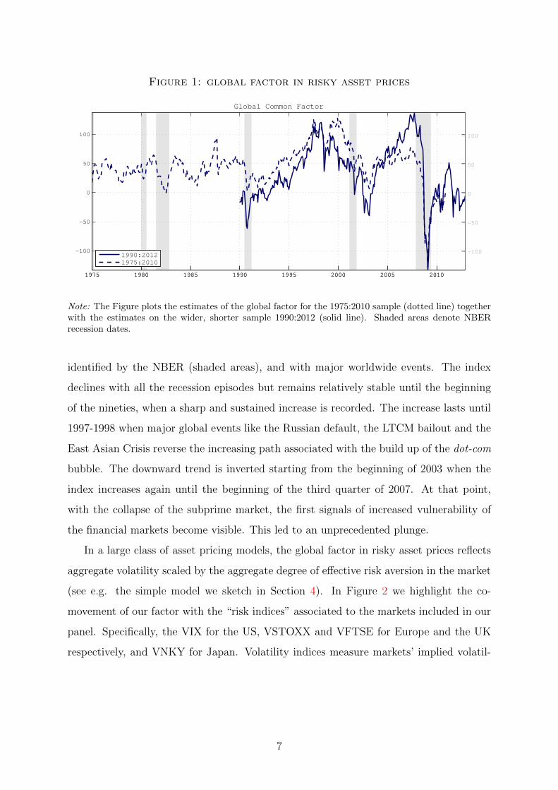
Figure 1: global factor in risky asset prices

1975 1980 1985 1990 1995 2000 2005 2010

−100

−50

0

50

100

Global Common Factor

1975 1980 1985 1990 1995 2000 2005 2010

−100

−50

0

50

100

1990:20121975:2010

Note: The Figure plots the estimates of the global factor for the 1975:2010 sample (dotted line) togetherwith the estimates on the wider, shorter sample 1990:2012 (solid line). Shaded areas denote NBERrecession dates.

identified by the NBER (shaded areas), and with major worldwide events. The index

declines with all the recession episodes but remains relatively stable until the beginning

of the nineties, when a sharp and sustained increase is recorded. The increase lasts until

1997-1998 when major global events like the Russian default, the LTCM bailout and the

East Asian Crisis reverse the increasing path associated with the build up of the dot-com

bubble. The downward trend is inverted starting from the beginning of 2003 when the

index increases again until the beginning of the third quarter of 2007. At that point,

with the collapse of the subprime market, the first signals of increased vulnerability of

the financial markets become visible. This led to an unprecedented plunge.

In a large class of asset pricing models, the global factor in risky asset prices reflects

aggregate volatility scaled by the aggregate degree of effective risk aversion in the market

(see e.g. the simple model we sketch in Section 4). In Figure 2 we highlight the co-

movement of our factor with the “risk indices” associated to the markets included in our

panel. Specifically, the VIX for the US, VSTOXX and VFTSE for Europe and the UK

respectively, and VNKY for Japan. Volatility indices measure markets’ implied volatil-

7

Figure 2: global factor and volatility indices

1990 2000 2010

0

1990 2000 2010

50

VIX

1990 2000 2010

−100

0

100

1990 2000 2010

20

40

60

VSTOXX

1990 2000 2010

0

1990 2000 2010

50

VFTSE

1990 2000 2010

0

1990 2000 2010

50

VNKY

Note: Clockwise from top-left panel, the global factor (solid line) together with major volatility indices(dotted lines): VIX (US), VSTOXX (EU), VNKY (JP) and VFTSE (UK). Shaded grey areas highlightNBER recession times.

ity, and thus reflect both the expectation of future market variance, and risk aversion.10

Therefore we expect all of them to be inversely related to our factor.11 We note that

the factor and the volatility indices display a remarkable common behaviour and peaks

consistently coincide within the overlapping samples. While the comparison with the

VIX is somehow facilitated by the length of the CBOE index, the same considerations

easily extend to all other indices analyzed. Comparison with the GZ-spread of Gilchrist

and Zakrajsek (2012) and the Baa-Aaa corporate bond spread (not reported) show that

these indices also display some commonalities, even if the synchronicity is slightly less

obvious than the one we find with respect to the implied volatilities.

Lastly, we separate the aggregate risk aversion and volatility components in our factor.

The construction of our proxy for aggregate risk aversion is modelled along the lines of

e.g. Bekaert et al. (2013) that estimate variance risk premia as the difference between a

measure of the implied variance (the squared VIX) and an estimated physical expected

10These indices are typically regarded as an instrument to assess the degree of strains and risk infinancial markets

11The estimated global factors are rotated such that they positively comove with prices; i.e. an increasein the index is interpreted as an increase in asset prices.

8

Figure 3: global factor decomposition

Credit Crunch: 434.7*

1990 1992 1994 1996 1998 2000 2002 2004 2006 2008 20100

50

100

150

200

250

Global Realized Variance

1990 1992 1994 1996 1998 2000 2002 2004 2006 2008 2010

-2

-1

0

1

2

3 Aggregate Risk Aversion Proxy

Note: [top panel] Monthly global realized variance measured using daily returns of the MSCI Index.The y axis is trimmed to enhance readability, during the credit crunch episode the index reached amaximum of 434.70. [bottom panel] Index of aggregate risk aversion calculated as (the inverse of) theresidual of the projection of the global factor onto the realized variance. Shaded grey areas highlightNBER recession times. Source: Global Financial Data and authors calculations.

variance which is primarily a function of realized variances. First, we obtain an estimate of

realized monthly global volatility using daily returns of the global MSCI Index.12 Second,

we calculate a proxy for aggregate risk aversion as the inverse of the centred residuals of

the projection of the global factor on the realized variance. The results of this exercise

are summarized in Figure 3. Our monthly measure of global realized variance is in the

top panel, while the implied index of aggregate risk aversion is in the bottom panel.

Very interestingly, the degree of market risk aversion that we recover from this simple

decomposition is in continuous decline between 2003 and the beginning of 2007, and it

decreases to very low levels, at a time where volatility was uniformly low and global

banks were prevalent and may have been the “marginal buyers” in international financial

markets. During that period, Shin (2012) documents the large share of banking flows

in aggregate capital flows. Changes in regulation and consequences of the crisis have

reduced the share of bank flows since 2008. We report data relative to aggregate capital

12We work under the assumption that monthly realized variances calculated summing over daily returnsprovide a sufficiently accurate proxy of realized variance at monthly frequency.

9

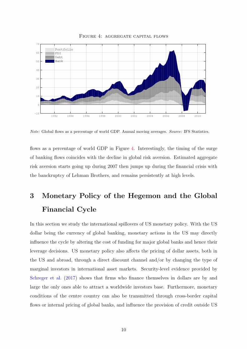
Figure 4: aggregate capital flows

1992 1994 1996 1998 2000 2002 2004 2006 2008 2010-10

0

10

20

30

40

50

60

70

PortfolioFDIDebtBank

Note: Global flows as a percentage of world GDP. Annual moving averages. Source: IFS Statistics.

flows as a percentage of world GDP in Figure 4. Interestingly, the timing of the surge

of banking flows coincides with the decline in global risk aversion. Estimated aggregate

risk aversion starts going up during 2007 then jumps up during the financial crisis with

the banckruptcy of Lehman Brothers, and remains persistently at high levels.

3 Monetary Policy of the Hegemon and the Global

Financial Cycle

In this section we study the international spillovers of US monetary policy. With the US

dollar being the currency of global banking, monetary actions in the US may directly

influence the cycle by altering the cost of funding for major global banks and hence their

leverage decisions. US monetary policy also affects the pricing of dollar assets, both in

the US and abroad, through a direct discount channel and/or by changing the type of

marginal investors in international asset markets. Security-level evidence provided by

Schreger et al. (2017) shows that firms who finance themselves in dollars are by and

large the only ones able to attract a worldwide investors base. Furthermore, monetary

conditions of the centre country can also be transmitted through cross-border capital

flows or internal pricing of global banks, and influence the provision of credit outside US

10

borders (see the corroborative evidence in Morais et al., 2015 for Mexico, and in Baskaya

et al., 2017 for Turkey).

Fluctuations in asset prices are both cause and consequence of the procyclicality of

financial leverage of global banks (see Section 4.2). Prolonged periods of loose monetary

policy may reduce market uncertainty and credit/funding costs, with a boost to asset

prices. Equally, rising asset prices may mask the fragile foundations of large and ex-

panding global banks’ balance sheets.13 Hence, the hegemon monetary policy may well

influence the global risk appetite of international markets.

To study the effects of US monetary policy on the Global Financial Cycle (GFC),

we devise a single framework that permits analyzing the transmission of monetary pol-

icy above and beyond national borders. We augment the typical set of macroeconomic

variables, output, inflation, investment, consumer sentiment and labor data, with global

financial variables, and study their joint dynamics in a medium scale Bayesian VAR.

There are a number of advantages that come with this choice. Most obviously, relying on

a unique specification permits addressing the effects of US monetary policy on the GFC

against the background of the response of the domestic business cycle. This acts both as

a complement to the analysis, and as a disciplining device to ensure that the identified

shock is in fact inducing responses that do not deviate from the standard channels of

domestic monetary transmission. Moreover, the dimensionality and composition of the

set of variables included in the VAR greatly reduce the problem of omitted variables

that generally plagues smaller systems and is likely to invalidate the identification of the

structural shocks.14 The argument in favour of small-scale systems typically levers on the

so-called curse of dimensionality: in an unrestricted VAR, the number of free parameters

to be estimated rapidly proliferates with the addition of extra variables, and the risks of

over-parametrization, and consequent high uncertainty around parameters estimates, are

a legitimate source of concern. In particular, with macroeconomic data being sampled

13For a model where low funding costs lower risk aversion and increase leverage see Coimbra and Rey(2017)

14Banbura et al. (2010) show that a medium-scale VAR of comparable size and composition to the oneused in this paper is able to correctly recover the shocks and reproduce responses that match theoreticalones. Intuitively, the large degree of comovement among macroeconomic variables makes it possible forVARs of such size to effectively summarize the information contained in large VARs typically countingover hundred variables.

11

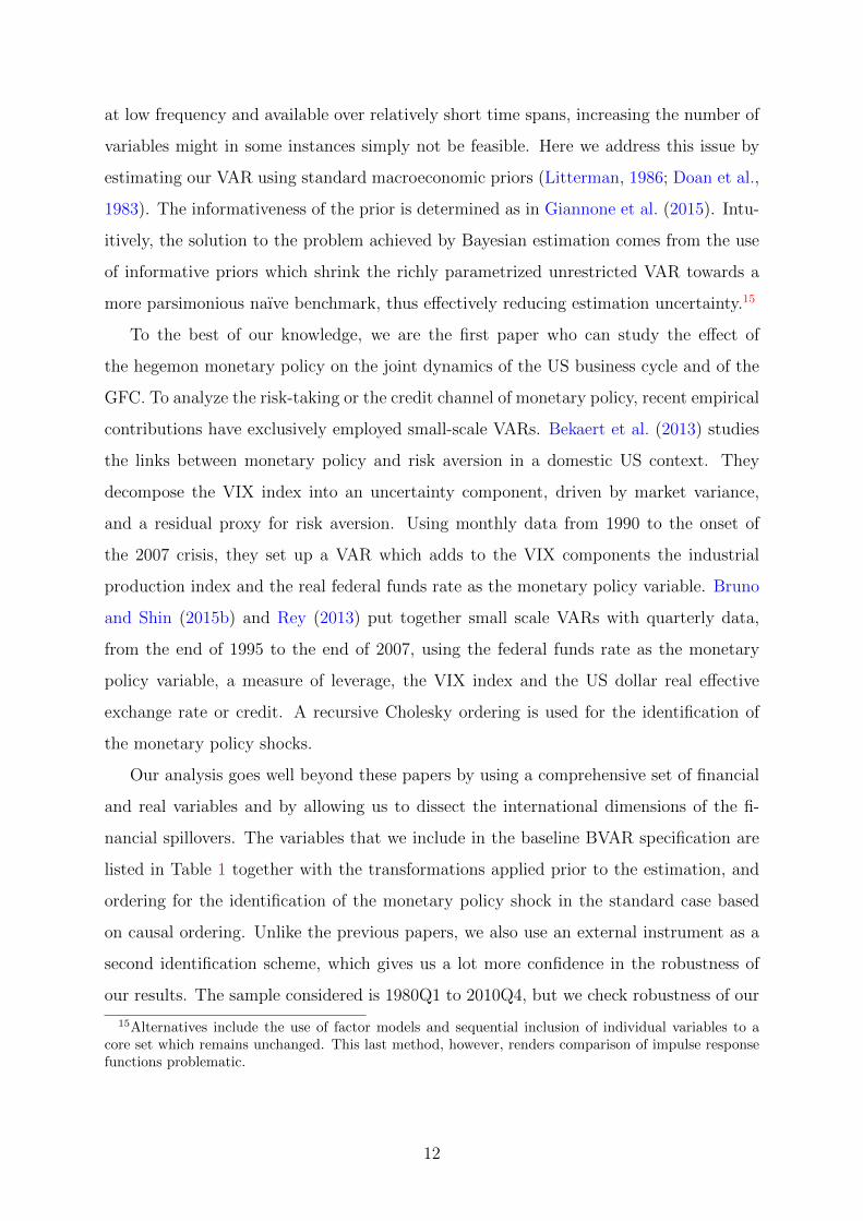
at low frequency and available over relatively short time spans, increasing the number of

variables might in some instances simply not be feasible. Here we address this issue by

estimating our VAR using standard macroeconomic priors (Litterman, 1986; Doan et al.,

1983). The informativeness of the prior is determined as in Giannone et al. (2015). Intu-

itively, the solution to the problem achieved by Bayesian estimation comes from the use

of informative priors which shrink the richly parametrized unrestricted VAR towards a

more parsimonious naıve benchmark, thus effectively reducing estimation uncertainty.15

To the best of our knowledge, we are the first paper who can study the effect of

the hegemon monetary policy on the joint dynamics of the US business cycle and of the

GFC. To analyze the risk-taking or the credit channel of monetary policy, recent empirical

contributions have exclusively employed small-scale VARs. Bekaert et al. (2013) studies

the links between monetary policy and risk aversion in a domestic US context. They

decompose the VIX index into an uncertainty component, driven by market variance,

and a residual proxy for risk aversion. Using monthly data from 1990 to the onset of

the 2007 crisis, they set up a VAR which adds to the VIX components the industrial

production index and the real federal funds rate as the monetary policy variable. Bruno

and Shin (2015b) and Rey (2013) put together small scale VARs with quarterly data,

from the end of 1995 to the end of 2007, using the federal funds rate as the monetary

policy variable, a measure of leverage, the VIX index and the US dollar real effective

exchange rate or credit. A recursive Cholesky ordering is used for the identification of

the monetary policy shocks.

Our analysis goes well beyond these papers by using a comprehensive set of financial

and real variables and by allowing us to dissect the international dimensions of the fi-

nancial spillovers. The variables that we include in the baseline BVAR specification are

listed in Table 1 together with the transformations applied prior to the estimation, and

ordering for the identification of the monetary policy shock in the standard case based

on causal ordering. Unlike the previous papers, we also use an external instrument as a

second identification scheme, which gives us a lot more confidence in the robustness of

our results. The sample considered is 1980Q1 to 2010Q4, but we check robustness of our

15Alternatives include the use of factor models and sequential inclusion of individual variables to acore set which remains unchanged. This last method, however, renders comparison of impulse responsefunctions problematic.

12

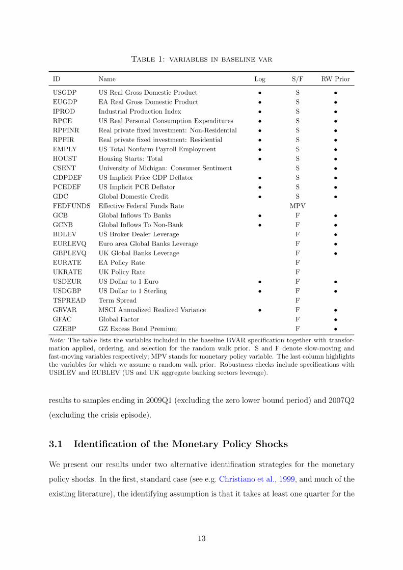
Table 1: variables in baseline var

ID Name Log S/F RW Prior

USGDP US Real Gross Domestic Product • S •EUGDP EA Real Gross Domestic Product • S •IPROD Industrial Production Index • S •RPCE US Real Personal Consumption Expenditures • S •RPFINR Real private fixed investment: Non-Residential • S •RPFIR Real private fixed investment: Residential • S •EMPLY US Total Nonfarm Payroll Employment • S •HOUST Housing Starts: Total • S •CSENT University of Michigan: Consumer Sentiment S •GDPDEF US Implicit Price GDP Deflator • S •PCEDEF US Implicit PCE Deflator • S •GDC Global Domestic Credit • S •FEDFUNDS Effective Federal Funds Rate MPV

GCB Global Inflows To Banks • F •GCNB Global Inflows To Non-Bank • F •BDLEV US Broker Dealer Leverage F •EURLEVQ Euro area Global Banks Leverage F •GBPLEVQ UK Global Banks Leverage F •EURATE EA Policy Rate F

UKRATE UK Policy Rate F

USDEUR US Dollar to 1 Euro • F •USDGBP US Dollar to 1 Sterling • F •TSPREAD Term Spread F

GRVAR MSCI Annualized Realized Variance • F •GFAC Global Factor F •GZEBP GZ Excess Bond Premium F •

Note: The table lists the variables included in the baseline BVAR specification together with transfor-mation applied, ordering, and selection for the random walk prior. S and F denote slow-moving andfast-moving variables respectively; MPV stands for monetary policy variable. The last column highlightsthe variables for which we assume a random walk prior. Robustness checks include specifications withUSBLEV and EUBLEV (US and UK aggregate banking sectors leverage).

results to samples ending in 2009Q1 (excluding the zero lower bound period) and 2007Q2

(excluding the crisis episode).

3.1 Identification of the Monetary Policy Shocks

We present our results under two alternative identification strategies for the monetary

policy shocks. In the first, standard case (see e.g. Christiano et al., 1999, and much of the

existing literature), the identifying assumption is that it takes at least one quarter for the

13

slow-moving variables such as output and prices (e.g. GDP and PCE deflator) to react to

monetary policy shocks, and that the monetary authority only sees past observations of

the fast-moving ones when making decisions. The identification in this case is practically

achieved by computing the Cholesky factor of the residual covariance matrix of the VAR

where variables enter following the order in Table 1. This identification scheme is useful

to compare relevant subsets of our results with the existing (smaller) VARs reported in

the literature.

The second identification scheme makes use of an external instrument to identify

the monetary policy shocks (Stock and Watson, 2012; Mertens and Ravn, 2013). The

intuition behind this approach to identification is that the mapping between the VAR

innovations and the structural shock of interest can be estimated using only moments of

observables, provided that a valid instrument for such shock exists. The contemporaneous

transmission coefficients are a function of the regression coefficients of the VAR residuals

onto the instrument, up to a normalization. Hence, given the instrument, this method

ensures that we can isolate the causal effects of a monetary policy shock on the dynamics

of our large set of variables without imposing any timing restrictions on the responses.

Technical details are discussed in Appendix D.

The crucial step of this identification strategy is, naturally, the choice of the instru-

ment. In Table 2 we summarize a series of tests which we use to guide our choice of the

preferred instrument. Conditional on the information set, sampling frequency and time

span of the baseline BVAR with 4 lags, we use (i) the F statistics of the regression of

the policy equation residuals (FEDFUNDS) on the instrument, and (ii) a measure of the

scalar reliability of the instrument, bounded between zero and 1, as discussed in Mertens

and Ravn (2013), together with 90% posterior confidence intervals.16

We consider a number of different candidate instruments, all intended to be a noisy

measure of the underlying monetary policy shocks. It is important to stress that these are

not supposed to be a perfect measure of the shock, nor are they supposed to be perfectly

correlated with it. As long as they can be thought of as exogenous with respect to other

16When the number of structural shocks of interest is equal to one, the statistical reliability is inter-preted as the fraction of the variance in the measured variable (i.e. the instrument) which is explainedby the latent shock, or, stated differently, it is the implied squared correlation between the instrumentand the latent structural shock (Mertens and Ravn, 2013).

14

shocks, and to display a non-negligible degree of correlation with the structural shock of

interest, then they can in principle be used to identify the shock. Our first candidate is a

narrative-based proxy (MPN) constructed extending the narrative shock first proposed in

Romer and Romer (2004) up to 2007, following the instructions detailed in Appendix D.

The variable captures the changes in the intended federal funds rate that are not taken

in response to the Fed’s forecasts about either current or future economic developments.

Other candidate instruments are instead constructed using market reactions to FOMC

announcements, and measured within a tight 30-minute window around the announce-

ments. We use the Target (FOMCF) and Path (PATHF) factors of Gurkaynak et al.

(2005), and their underlying components, whose use as instruments for the monetary

policy shock was first introduced, at monthly frequency, in Gertler and Karadi (2015).17

In Table 2, MP1 and FF4 are the monetary surprises implied by changes in the current-

month and the three-months-ahead federal funds futures respectively, while ED2, ED3

and ED4 are the surprises in the second, third, and fourth eurodollar futures contracts,

which have 1.5, 2.5, and 3.5 quarters to expiration on average. The Target and Path

factors are obtained as a rotation of the first two principal components of the surprises in

the five contracts above. The rotation is such that the Target factor is interpreted as the

surprise changes in the current federal fund rate target, while the Path factor measures

changes in the future path of policy which are orthogonal to changes in the current target

interest rate (see Gurkaynak et al., 2005). We construct quarterly surprises as the sum

of daily data.

We follow Stock et al. (2002) and require the F statistic to be above ten, for the instru-

ment not to be weak. The numbers in Table 2 show that the narrative-based instrument

is the only one which is safely above the threshold. All the market-based surprises are

well below the critical value, notwithstanding comparable levels of reliability. These num-

bers confirm the findings of Stock and Watson (2012). It is also worth stressing that the

numbers reported relate to the relevance of the instruments, while they remain silent on

their exogeneity. Miranda-Agrippino (2016); Miranda-Agrippino and Ricco (2017) dis-

cuss the informational content of market-based monetary surprises and show that while

17Other applications of high-frequency futures data to the transmission of monetary policy shocks in-clude, among others, Nakamura and Steinsson (2017) and Krishnamurthy and Vissing-Jorgensen (2011).

15

they successfully capture the component of policy that is unexpected by market partic-

ipants, they map into the shocks only under the assumption that markets can correctly

and immediately disentangle the systematic component of policy from any observable

policy action. In the presence of information frictions, the high-frequency surprises are

also a function of the information about economic fundamentals that the central bank

implicitly discloses at the time of the policy announcements.18 Failure to account for

this effect hinders the correct identification of the shocks, resulting in severe price and

real activity puzzles. We confirm this finding also in our quarterly setting. This issue is

likely to be mitigated in our framework, due to the large information set included in our

VAR. However, we still find that the responses obtained using market-based instruments

tend to be more unstable, and hence only report results obtained using high-frequency

instruments in the appendix.19 Hence, we use the narrative-based series as the preferred

instrument.

3.2 Discussion of the Results

Figures (6) to (10) collect the responses of our variables of interest to a contractionary

US monetary policy shock. These summarize the effects of US monetary policy on the

Global Financial Cycle. Figure (5) displays IRFs of a subset of domestic business cycle

variables. The full set of responses is in Figure (E.1). The impulse response functions

(IRFs) are obtained by estimating a VAR(4).20 The responses are normalized such that

the shock induces a 100bp increase in the effective federal funds rate. We compare

responses obtained using the recursive identification scheme (red, solid) to those obtained

using the narrative series as an external instrument (blue, dash-dotted). For the recursive

identification we plot modal responses to the monetary policy shock together with 68%

18The implicit disclosure of information is the Fed information effect in Nakamura and Steinsson (2017),and the signalling channel of monetary policy discussed in Melosi (2017).

19 In an additional exercise, we use the quarterly MP1 and Target factor (the market-based instrumentswith the largest F statistic) to identify the shock as follows: (1) calculate the F statistic for each drawof the VAR innovations; (2) retain contemporaneous transmission coefficients associated to F statisticslarger than 10; (3) use the median of the retained draws for the responses. IRFs obtained in this way arelargely consistent with the ones reported below, and are collected in Figures E.5 and E.6 in AppendixE. However, we note that the number of draws for which the F statistic is larger than 10 is less than 3%of the total: 64 (MP1) and 33 (FOMCF) draws out of 2500.

20Using 3 and 5 lags leads to virtually identical responses. See Appendix C for a detailed descriptionof the estimation and priors used.

16

Table 2: tests for instruments relevance

instrument F stat 90% posterior ci reliability 90% posterior ci

MPN 16.225 [4.578 21.120] 0.2715 [0.192 0.356]

FOMCF 5.801 [0.669 7.756] 0.2835 [0.195 0.379]

PATHF 0.027 [0.007 2.298] 0.2806 [0.133 0.371]

MP1 4.718 [1.103 8.858] 0.2689 [0.188 0.355]

FF4 4.643 [0.113 5.444] 0.2298 [0.143 0.319]

ED2 3.190 [0.033 3.785] 0.2649 [0.158 0.360]

ED3 1.551 [0.006 2.536] 0.2146 [0.110 0.304]

ED4 1.527 [0.003 1.804] 0.2025 [0.103 0.293]

Note: For each of the candidate instruments the table reports the F statistics associated to the firststage regression of the VAR policy innovation onto the instrument, a measure of statistical reliability,bounded between zero and 1 together with 90% posterior coverage intervals. Candidate instruments are:a narrative-based measure of monetary surprises constructed extending the work of Romer and Romer(2004) up to 2007 and 2009 (first two rows); the Target and Path factors of Gurkaynak et al. (2005),and the surprises in the current-month (MP1) and three-months-ahead (FF4) federal fund futures, andin the second (ED2), third (ED3) and fourth (ED4) eurodollar futures. VAR innovations are from aBVAR(4) on the variables listed in Table 1 from 1980Q1 to 2010Q4.

and 90% posterior coverage bands (grey shaded areas). For the identification with the

narrative instrument we report median responses for the retained draws for which the

first-stage F statistic is at least equal to 10. Dashed lines are 68% intervals from the

distribution of the retained draws. Results are robust to a number of changes in the VAR

lag structure, set composition, and length of the sample considered, for which additional

charts are reported in Appendix E at the end of the paper.

The responses of US variables to a monetary policy shock and subsequent dynamics

are consistent with textbook economic theory, and qualitatively similar under both identi-

fication schemes (see also Figure E.1). Output, production and consumption all contract,

and so do private residential and non-residential investments, and non farm payroll em-

ployment. European GDP increases slightly in response to the US shock, possibly due to

an expenditure switching effect, and then contracts with delay. There is no price puzzle:

price inflation whether measured by the GDP deflator or the PCE deflator goes down.

Consumer sentiment declines. The responses of domestic variables to a contractionary

monetary policy shock are thus coherent with the theoretical effects of monetary policy:

following an unexpected tightening by the Fed, we witness a contraction of national real

17

Figure 5: responses of domestic business cycle

Real GDP

0 4 8 12 16 20

-8

-6

-4

-2

0

Real PersonalConsumption Expenditures

0 4 8 12 16 20

-8

-6

-4

-2

0

Real Non-ResidentialInvestments

0 4 8 12 16 20

-10

-5

0

5

Real ResidentialInvestments

0 4 8 12 16 20

-20

-10

0

Non-Farm PayrollEmployment

0 4 8 12 16 20

-4

-2

0

Consumer Sentiment

0 4 8 12 16 20-4

-2

0

GDP Deflator

0 4 8 12 16 20

-6

-4

-2

0

PCE Deflator

0 4 8 12 16 20

-6

-4

-2

0

Fed Funds Rate

0 4 8 12 16 20

0

0.5

1

CholeskyNarrative

Note: Responses to a US contractionary monetary policy shock that induces a 1% increase in the fedfunds rate. [red lines and grey areas] Recursive identification with 68% and 90% posterior coveragebands. [blue lines] Identification with narrative series as external instrument and 68% intervals.

activity and prices. Furthermore, consumption and income decrease as do investment

and consumers sentiment. This gives us confidence in the reliability of our identifica-

tion scheme. We now turn to the main added value of our analysis which is the joint

dynamics of global financial variables following a tightening in the centre country of the

international monetary system (the US) and zoom on four subsets of those.

First, we look at credit provision both domestically and internationally (Figures 6 and

7). We compute global variables as the cross-sectional sum of country-specific equivalents

which are in turn constructed following the instructions detailed in Appendix A. Global

inflows are direct cross-border credit flows provided by foreign banks to both banks and

non-banks in the recipient country (Avdjiev et al., 2012). Second, we look at banks’

leverage (Figure 8). We separate global banks from the aggregate banking sector, due

18

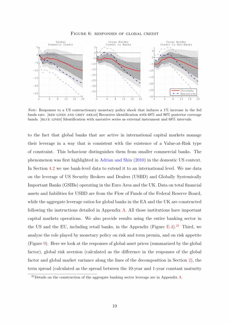
Figure 6: responses of global credit

GlobalDomestic Credit

0 4 8 12 16 20

−25

−20

−15

−10

−5

0

5

Cross BorderCredit to Banks

0 4 8 12 16 20

−35

−30

−25

−20

−15

−10

−5

0

5

Cross BorderCredit to Non−Banks

0 4 8 12 16 20−30

−25

−20

−15

−10

−5

0

5

CholeskyNarrative


to the fact that global banks that are active in international capital markets manage

their leverage in a way that is consistent with the existence of a Value-at-Risk type

of constraint. This behaviour distinguishes them from smaller commercial banks. The

phenomenon was first highlighted in Adrian and Shin (2010) in the domestic US context.

In Section 4.2 we use bank-level data to extend it to an international level. We use data

on the leverage of US Security Brokers and Dealers (USBD) and Globally Systemically

Important Banks (GSIBs) operating in the Euro Area and the UK. Data on total financial

assets and liabilities for USBD are from the Flow of Funds of the Federal Reserve Board,

while the aggregate leverage ratios for global banks in the EA and the UK are constructed

following the instructions detailed in Appendix A. All those institutions have important

capital markets operations. We also provide results using the entire banking sector in

the US and the EU, including retail banks, in the Appendix (Figure E.4).21 Third, we

analyze the role played by monetary policy on risk and term premia, and on risk appetite

(Figure 9). Here we look at the responses of global asset prices (summarized by the global

factor), global risk aversion (calculated as the difference in the responses of the global

factor and global market variance along the lines of the decomposition in Section 2), the

term spread (calculated as the spread between the 10-year and 1-year constant maturity

21Details on the construction of the aggregate banking sector leverage are in Appendix A.

19

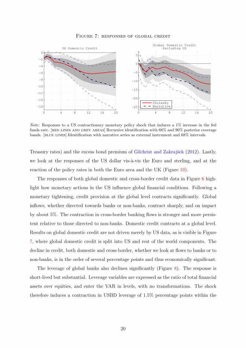
Figure 7: responses of global credit

US Domestic Credit

0 4 8 12 16 20

−16

−14

−12

−10

−8

−6

−4

−2

0

Global Domestic CreditExcluding US

0 4 8 12 16 20

−25

−20

−15

−10

−5

0

5

CholeskyNarrative


Treasury rates) and the excess bond premium of Gilchrist and Zakrajsek (2012). Lastly,

we look at the responses of the US dollar vis-a-vis the Euro and sterling, and at the

reaction of the policy rates in both the Euro area and the UK (Figure 10).

The responses of both global domestic and cross-border credit data in Figure 6 high-

light how monetary actions in the US influence global financial conditions. Following a

monetary tightening, credit provision at the global level contracts significantly. Global

inflows, whether directed towards banks or non-banks, contract sharply, and on impact

by about 5%. The contraction in cross-border banking flows is stronger and more persis-

tent relative to those directed to non-banks. Domestic credit contracts at a global level.

Results on global domestic credit are not driven merely by US data, as is visible in Figure

7, where global domestic credit is split into US and rest of the world components. The

decline in credit, both domestic and cross-border, whether we look at flows to banks or to

non-banks, is in the order of several percentage points and thus economically significant.

The leverage of global banks also declines significantly (Figure 8). The response is

short-lived but substantial. Leverage variables are expressed as the ratio of total financial

assets over equities, and enter the VAR in levels, with no transformations. The shock

therefore induces a contraction in USBD leverage of 1.5% percentage points within the

20

Figure 8: responses of leverage of global banks

US Broker−DealersLeverage

0 4 8 12 16 20−3

−2.5

−2

−1.5

−1

−0.5

0

0.5

1

1.5

2

EA G−SIBsLeverage

0 4 8 12 16 20

−0.6

−0.5

−0.4

−0.3

−0.2

−0.1

0

0.1

0.2

0.3

0.4

UK G−SIBsLeverage

0 4 8 12 16 20−0.8

−0.6

−0.4

−0.2

0

0.2

0.4

0.6

CholeskyNarrative


first year. The leverage of European (EA and UK) global banks also contracts, and with

similar dynamics. The banking sector as a whole reacts more sluggishly, and in fact

registers an initial increase in the median leverage ratio (see Figure E.4 of the Appendix)

before contracting. Domestically oriented retail banks take longer to adjust, so that

broader banking aggregates only react with a delay to monetary policy shocks, which

instead affects more immediately the large banks with important capital market opera-

tions. Overall, global banks seem to respond more quickly to changes in the monetary

policy stance. This is consistent with these institutions being more reactive to financing

conditions when adjusting leverage.

Following a contractionary US monetary policy shock global financial markets also

suffer a contraction (Figure 9). The global factor in world risky asset prices declines

significantly. Using the decomposition in Section 2 we recover the response of global

risk aversion as the difference between the responses of the global factor (inverted) and

of global market volatility.22 Our results point towards a significant impact rise in the

aggregate degree of risk aversion in global financial markets following a monetary policy

contraction in the centre country. Risk premia also increase on impact, confirming the

existence of a financial channel for monetary policy which directly influences borrowing

22Posterior coverage bands are obtained by computing the implied response of risk aversion at eachdraw of the parameters under the recursive identification scheme.

21

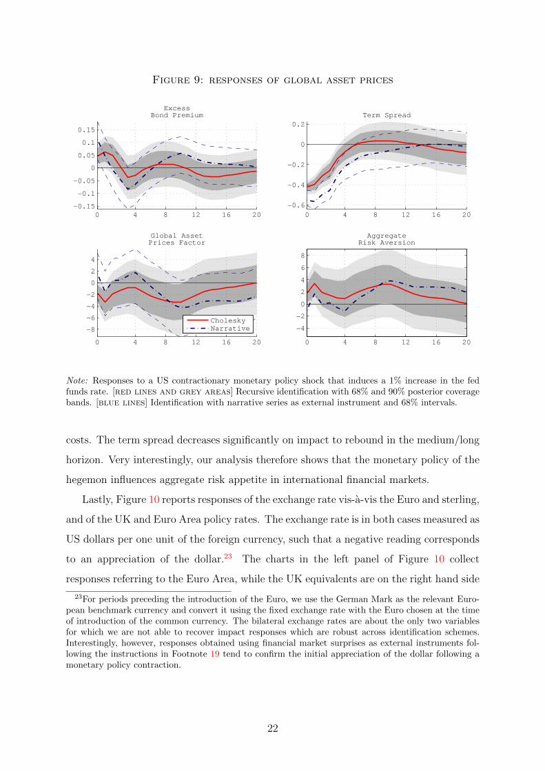
Figure 9: responses of global asset prices

ExcessBond Premium

0 4 8 12 16 20−0.15

−0.1

−0.05

0

0.05

0.1

0.15

Term Spread

0 4 8 12 16 20−0.6

−0.4

−0.2

0

0.2

Global AssetPrices Factor

0 4 8 12 16 20

−8

−6

−4

−2

0

2

4

AggregateRisk Aversion

0 4 8 12 16 20

−4

−2

0

2

4

6

8

CholeskyNarrative


costs. The term spread decreases significantly on impact to rebound in the medium/long

horizon. Very interestingly, our analysis therefore shows that the monetary policy of the

hegemon influences aggregate risk appetite in international financial markets.

Lastly, Figure 10 reports responses of the exchange rate vis-a-vis the Euro and sterling,

and of the UK and Euro Area policy rates. The exchange rate is in both cases measured as

US dollars per one unit of the foreign currency, such that a negative reading corresponds

to an appreciation of the dollar.23 The charts in the left panel of Figure 10 collect

responses referring to the Euro Area, while the UK equivalents are on the right hand side

23For periods preceding the introduction of the Euro, we use the German Mark as the relevant Euro-pean benchmark currency and convert it using the fixed exchange rate with the Euro chosen at the timeof introduction of the common currency. The bilateral exchange rates are about the only two variablesfor which we are not able to recover impact responses which are robust across identification schemes.Interestingly, however, responses obtained using financial market surprises as external instruments fol-lowing the instructions in Footnote 19 tend to confirm the initial appreciation of the dollar following amonetary policy contraction.

22

Figure 10: responses of currency and policy rates

USD to 1 EUR

0 4 8 12 16 20

−10

−5

0

5

10

USD to 1 GBP

0 4 8 12 16 20

−5

0

5

10

15

ECB policy rate

0 4 8 12 16 20

−0.2

−0.1

0

0.1

0.2

0.3

0.4

BoE policy rate

0 4 8 12 16 20

−0.4

−0.2

0

0.2

0.4

0.6

CholeskyNarrative


of the figure. The overall qualitative shape of the responses is quite similar in the two

countries. There are, however, interesting differences. Following the shock, the dollar

appreciates significantly, and on impact, vis-a-vis the Euro. The response is relatively

short-lived, and the exchange rate goes back to trend within a year. With respect to

sterling, there seems to be no appreciable effect for the first few quarters, following which

the dollar depreciates. Notwithstanding the flexibility of the two exchange rates, our

results suggest that a contractionary move in the US is likely to be followed by tighter

monetary policies both in the UK and the Euro Area. Increases in the policy rates

are both positive and significant, and peak to about 50 and 20bp respectively, within

the first year after the shock. Interestingly, while the response of the European rate is

muted on impact, the UK policy rate jumps on impact by about 20bp. These results are

consistent with both a “fear of floating” argument (see Calvo and Reinhart, 2002), and

23

with endogenous developments in the UK and European economies. Hence, even with

fully flexible exchange rates, both the Euro Area and the UK respond to the US tightening

by raising their domestic policy rates as well. These results are also consistent with the

dilemma hypothesis put forward in Rey (2013). With mobile cross-border capital flows,

a fully flexible exchange rate is not necessarily enough to fully insulate countries against

the spillovers of foreign monetary policy shocks.

While we display results obtained estimating the BVAR using data up to 2010Q4, we

verify that our conclusions are not driven by the crisis episode of 2007/2008 by repeating

the estimation using data only up to 2007Q2 (Figure E.2). Responses are computed again

using both identification schemes discussed above and are virtually identical to the ones

presented.24 This seems to imply that the 2007 financial crisis, while having had unques-

tionable disruptive effects on the financial markets and having been followed by severe

recession episodes worldwide, has not in fact altered the fundamental macroeconomic

dynamics and transmission mechanisms both at the national and international levels. A

similar conclusion has been reached using national US data by Stock and Watson (2012).

Lastly, we look at the forecast error variance decomposition for a selection of the

variables included in the BVAR (Table C.1).25 We find that US monetary policy explains

a non trivial fraction of the forecast error variance of banks’ leverage, credit flows and

financial markets-related variables. At 1 year horizon, US monetary policy shocks explain

about 5% of the forecast error variance for cross border credit flows, and up to 12% at a

4 year horizon. It explains 2 or 3% of the forecast error variance of leverage at the 1 year

horizon. We also find that the variance of GDP and inflation explained by the monetary

policy shock increases with the horizon. In the long run, monetary policy shocks explain

about 3.5% of inflation variance, and 17 % of domestic GDP. Importantly, is also explains

over 14% of the variance of global banking flows at the same horizon.

24In fact, it is very hard to see the difference between the two sets of IRFs except for the exchangerates: the initial appreciation of the dollar tends to be more precisely estimated in Figure E.2. Resultsare also robust to ending the sample at the beginning of the zero lower bound period (not reported).

25While some of the numbers may seem small at a first glance, it is important to note that the shareof explained variance is reduced in rich information VARs, such as ours.

24

4 Interpretation

4.1 A Simple Model with Heterogeneous Investors

The empirical results show that US monetary policy affects global banks’ leverage, credit

creation around the world, capital flows, risky asset prices and global risk aversion. We

present a stylized model which features investors with heterogeneous risk taking propen-

sities to make sense of the time varying degree of aggregate effective risk aversion. As the

relative wealth of investors fluctuates, asset pricing will be determined mostly by one type

of investor or the other. Since the 1990s, world asset markets have become increasingly

integrated with large cross-border credit, equity and bond portfolio flows. Global banks

and asset managers have played an important role in this process of internationalization

and account for a large part of these flows. The share of credit in international flows has

risen during that period and decreased since 2008 as shown in Figure 4. Bank flows were

about 4% of world GDP at the beginning of the year 2000 and they grew to about 30%

of world GDP end 2007. During the same period, portfolio debt flows went from about

6% to 15% and portfolio equity flows remained at around 5%. We present an illustra-

tive model of international asset pricing where the risk premium depends on the wealth

distribution between leveraged global banks on the one hand, and asset managers, such

as insurance companies or sovereign wealth funds, on the other. The model presented in

this section is stylized and only here to help us interpret the data.26

The model builds directly on the work of Zigrand et al. (2010) and Adrian and Shin

(2014).27 We consider a world in which there are two types of investors: global banks and

asset managers. Global banks are leveraged entities that fund themselves in dollars for

their operations in global capital markets. They can borrow at the US risk-free rate and

lever to buy a portfolio of world risky securities, whose returns are in dollars. They are

risk-neutral investors and subject to a Value-at-Risk (VaR) constraint, which is imposed

on them by regulation.28 We present microeconomic evidence pertaining to the leverage

26For a more realistic dynamic stochastic general equilibrium model of asset pricing with heterogeneousinvestors and monetary policy see Coimbra and Rey (2017). Other types of model which generate timevarying risk aversion are for example models with consumption habit (see Campbell and Cochrane (1999))

27See also Etula (2013).28Their risk neutrality is an assumption which may be justified by the fact that they benefit from an

implicit bailout guarantee, either because they are universal banks, and are therefore part of a deposit

25

and risk taking behaviour of banks in Section 4.2.

The second type of investors are asset managers who, like global banks, acquire risky

securities in world markets and can borrow at the US risk-free rate. Asset managers also

hold a portfolio of regional assets (for example regional real estate) which is not traded

in financial markets, perhaps because of information asymmetries. Asset managers are

standard mean-variance investors and exhibit a positive degree of risk aversion that limits

their desire to leverage.29

Global Banks

Global banks maximize the expected return of their portfolio of world risky assets subject

to a Value-at-Risk constraint.30 The VaR imposes an upper limit on the amount a bank

is predicted to lose on a portfolio with a certain probability. We denote by Rt the vector

of excess returns in dollars of all traded risky assets in the world. We denote by xBt the

portfolio shares of a global bank. We call wBt the equity of the bank. The maximization

problem of a global bank is

maxxBt

Et(xB′t Rt+1

)subject to V aRt ≤ wBt ,

with the V aRt defined as a multiple α of the standard deviation of the bank portfolio

V aRt = αwBt[Vart

(xB′t Rt+1

)] 12

Taking the first order condition and using the fact that the constraint is binding (since

banks are risk neutral) gives the following solution for the vector of asset demands:

xBt =1

αλt[Vart(Rt+1)]−1 Et(Rt+1). (1)

guarantee scheme, or because they are too big to fail. Whatever the microfoundations, the crisis hasprovided ample evidence that global banks have taken on large amounts of risk and levered massively.

29The fact that only asset managers, and not the global banks, have a regional portfolio is non essential;global banks could be allowed to hold a portfolio of regional loans or assets as well. The asymmetryin risk aversion (risk neutral banks with VaR constraint and risk averse asset managers), however, isimportant for the results.

30VaR constraints have been used internally for the risk management of large banks for a long timeand have entered the regulatory sphere with Basel II and III. For a microfoundation of VaR constraints,see Adrian and Shin (2014).

26

This is formally similar to the portfolio allocation of a mean variance investor. In Eq. (1),

λt is the Lagrange multiplier: the VaR constraint plays the same role as risk aversion.31

Asset Managers

Asset managers are standard mean-variance investors with degree of risk aversion σ.

They have access to the same set of traded assets as global banks. We call xIt the vector

of portfolio weights of the asset managers in tradable risky assets. Asset managers also

invest in local (regional) non traded assets. We denote by yIt the fraction of their wealth

invested in those regional assets. The vector of excess returns on these non tradable

investments is RNt . Finally, we call wIt the equity of asset managers. An asset manager

chooses his portfolio of risky assets by maximizing

maxxIt

Et(xI′t Rt+1 + yI′t RN

t+1

)− σ

2Vart

(xI′t Rt+1 + yI′t RN

t+1

).

The optimal portfolio choice in risky tradable securities for an asset manager will be

xIt =1

σ[Vart(Rt+1)]−1 [Et(Rt+1)− σCovt(Rt+1,R

Nt+1)yIt

]. (2)

Market clearing conditions

The market clearing condition for risky traded securities is xBtwB

t

wBt +wI

t+ xIt

wIt

wBt +wI

t= st

where st is a world vector of net asset supplies for traded assets.

Proposition 1 (Risky Asset Returns) Using Eq. (1) and (2) and the market clear-

ing conditions, the expected excess returns on tradable risky assets can be rewritten as the

sum of a global component (aggregate variance scaled by aggregate effective risk aversion)

and a regional component:

Et (Rt+1) = ΓtVart(Rt+1) st + ΓtCovt(Rt+1,RNt+1)yt, (3)

where Γt ≡[wB

t

αλt+

wIt

σ

]−1 (wBt + wIt

).

31It is possible to solve out for the Lagrange multiplier using the binding VaR constraint (see Zigrand

et al., 2010). We find λt = [Et(Rt+1)′ [Vart(Rt+1)]−1 Et(Rt+1)]−1/2.

27

Γt is the wealth-weighted average of the “risk aversions” of asset managers and of the

global banks. It can thus be interpreted as the aggregate degree of effective risk aversion

of the market. If all the wealth were in the hands of asset managers, for example,

aggregate risk aversion would be equal to σ. The empirical counterpart of Eq. (3) is

the decomposition of risky asset returns into a global component (also a function of

the aggregate degree of risk aversion) and a regional component shown in Section 2. One

possible interpretation of the decline in aggregate effective risk aversion observed between

2003 and 2007 in Figure 3 is therefore that as global banks become large, they are more

important for the pricing of risky assets, and aggregate risk aversion goes down. This

trend is reversed after the crisis, when instead asset managers become relatively bigger.

Proposition 2 (Global Banks Returns) The expected excess return of a global bank

portfolio in our economy is given by

Et(xB′t Rt+1) = ΓtCovt(xB′t Rt+1, s′tRt+1) + ΓtCovt(xB′t Rt+1,y

′tR

Nt+1)

= βBWt Γt + ΓtCovt(xB′t Rt+1,y′tR

Nt+1), (4)

where βBWt is the beta of a global bank with the world market.

The more correlated a global bank portfolio with the world portfolio, the higher the

expected asset return, ceteris paribus. The high-βBWt global banks are the ones loading

more on world risk. The excess return is scaled up by the global degree of risk aversion

in the economy – Γt.

4.2 Evidence on Global Banks

Using US data on quarterly growth rates of both total assets and leverage (defined as

total assets over equity, measured at book value), Adrian and Shin (2010) show that

the positive association between leverage and size of balance sheets (in growth rate) is a

particular feature of broker-dealers, which distinguishes them from retail banks and from

households. Using balance sheet data for the same international sample of financial insti-

tutions we used in Section 3, we show in Figure A.3 that the positive association between

leverage and size of assets goes well beyond the US borders. We calculate leverage along

28

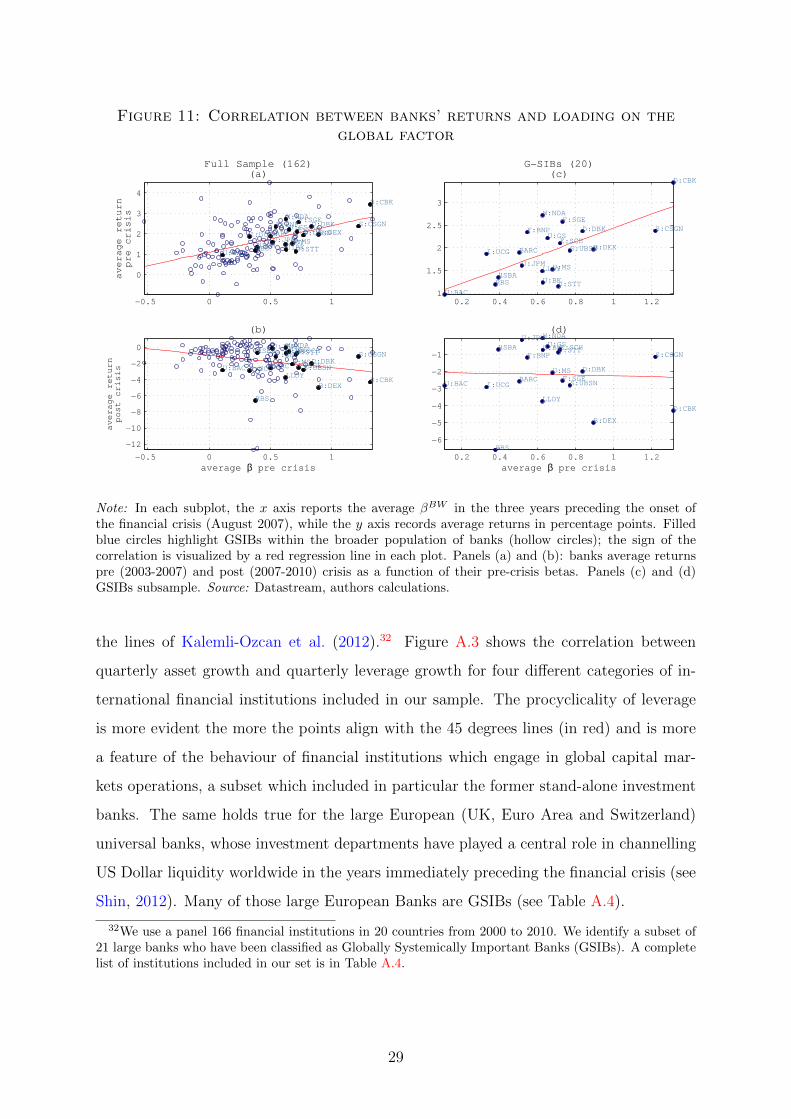
Figure 11: Correlation between banks’ returns and loading on theglobal factor

−0.5 0 0.5 1

0

1

2

3

4

B:DEX

HSBA LLOYBARC

RBS

I:UCG

F:SGEF:BNP D:DBK

D:CBK

E:SCH

W:NDAS:CSGN

S:UBSN

U:BACU:BK

U:GS

U:JPMU:MSU:STT

ave

rag

e r

etu

rnp

re c

risi

s

Full Sample (162)(a)

−0.5 0 0.5 1

−12

−10

−8

−6

−4

−2

0

B:DEX

HSBA

LLOYBARC

RBS

I:UCG F:SGE

F:BNPD:DBK

D:CBK

E:SCHW:NDA

S:CSGN

S:UBSNU:BAC

U:BKU:GSU:JPM

U:MSU:STT

average β pre crisis

ave

rag

e r

etu

rnp

ost

crisi

s

(b)

0.2 0.4 0.6 0.8 1 1.21

1.5

2

2.5

3

B:DEX

HSBALLOY

BARC

RBS

I:UCG

F:SGE

F:BNP D:DBK

D:CBK

E:SCH

W:NDA

S:CSGN

S:UBSN

U:BAC

U:BK

U:GS

U:JPM U:MS

U:STT

G−SIBs (20)(c)

0.2 0.4 0.6 0.8 1 1.2

−6

−5

−4

−3

−2

−1

B:DEX

HSBA

LLOY

BARC

RBS

I:UCGF:SGE

F:BNP

D:DBK

D:CBK

E:SCH

W:NDA

S:CSGN

S:UBSNU:BAC

U:BKU:GSU:JPM

U:MS

U:STT

average β pre crisis

(d)

Note: In each subplot, the x axis reports the average βBW in the three years preceding the onset ofthe financial crisis (August 2007), while the y axis records average returns in percentage points. Filledblue circles highlight GSIBs within the broader population of banks (hollow circles); the sign of thecorrelation is visualized by a red regression line in each plot. Panels (a) and (b): banks average returnspre (2003-2007) and post (2007-2010) crisis as a function of their pre-crisis betas. Panels (c) and (d)GSIBs subsample. Source: Datastream, authors calculations.

the lines of Kalemli-Ozcan et al. (2012).32 Figure A.3 shows the correlation between

quarterly asset growth and quarterly leverage growth for four different categories of in-

ternational financial institutions included in our sample. The procyclicality of leverage

is more evident the more the points align with the 45 degrees lines (in red) and is more

a feature of the behaviour of financial institutions which engage in global capital mar-

kets operations, a subset which included in particular the former stand-alone investment

banks. The same holds true for the large European (UK, Euro Area and Switzerland)

universal banks, whose investment departments have played a central role in channelling

US Dollar liquidity worldwide in the years immediately preceding the financial crisis (see

Shin, 2012). Many of those large European Banks are GSIBs (see Table A.4).

32We use a panel 166 financial institutions in 20 countries from 2000 to 2010. We identify a subset of21 large banks who have been classified as Globally Systemically Important Banks (GSIBs). A completelist of institutions included in our set is in Table A.4.

29

Figure 11 is the empirical counterpart of Eq. (4). It reports the correlation between

the returns of each bank and their loadings βBWt on the global risk factor of Section 2,

calculated over the entire population of banks – panels (a) and (b) –, and the GSIBs

subsample – panels (c) and (d) – respectively. We use August 2007 as a break point

to distinguish between pre and post crisis periods. Results indicate, as expected, a

positive correlation between loading up on systemic risk before the crisis and getting

high returns. Panels (a) and (c) show that, relative to the larger population, GSIBs tend

to have both higher average betas and larger returns. This suggests that global banks

were systematically loading more on world risk in the run-up to the financial crisis, and

that their behaviour was delivering larger average returns, compared to the average bank

in our sample. The higher loadings on risk are consistent with the build-up of leverage in

the years prior to the crisis documented in Figure A.2. Furthermore, panels (b) and (d)

sort the banks on the x-axis according to their pre-crisis betas, but report their post crisis

returns on the y axis. The charts show how the institutions that were loading more on

global risk pre crisis suffered the largest losses after the systemic meltdown. The micro

data on global banks are therefore consistent with US monetary policy being transmitted

internationally through the financial system.

5 Conclusions

This paper establishes the importance of US monetary policy as one of the drivers of the

Global Financial Cycle. The hegemon monetary policy influences global risk appetite.

First, we show that one global factor explains an important part of the variance of a

large cross section of returns of risky asset prices around the world. This factor can be

interpreted as reflecting movements in aggregate volatility on world equity markets, and

time-varying market-wide risk aversion. We find in particular evidence of a significant

decline in effective risk aversion between 2003 and the beginning of 2007, that is during

the crisis build up phase. That period matches the increased importance of global banks

in international capital markets. Second, we investigate the links of the Global Financial

Cycle with US monetary policy, as the dollar is an important funding currency for global

30

intermediaries, and a large portion of portfolios worldwide are denominated in dollars.33

Because we use a medium-scale Bayesian VAR and a robust identification method, we

believe we are the first paper able to look meaningfully at the joint behaviour of the

domestic business cycle and international financial variables in a single comprehensive

modelling framework. Responses to a monetary policy shock in the US are identified using

a standard recursive scheme, and a narrative measure of monetary policy disturbances a

la Romer and Romer (2004) as an external instrument.

We find evidence of powerful monetary policy spillovers from the US to the rest of

the world. When the US Federal Reserve tightens, domestic output, investment, and

inflation contract. But, importantly, we also see significant movements in international

financial variables: the global factor in asset prices goes down, spreads go up, global

domestic and cross-border credit go down significantly and leverage decreases, first among

US broker-dealers and for global banks in the Euro area and the UK, then among the

broader banking sector in the US and in Europe. We also find evidence of an endogenous

reactions of monetary policy rates in the UK and in the Euro area. Hence, we find that

US monetary policy is a driver of the Global Financial Cycle.34 This is an important

result as it challenges the degree of monetary policy independence enjoyed by countries

around the world, even those who have flexible exchange rates such as the UK or the

Euro Area. This fits with the claim of Rey (2013) that the Mundellian trilemma may

have really morphed into a dilemma: as long as capital flows across borders are free and

macro prudential tools are not used to control credit growth, monetary conditions in any

country, even one with a flexible exchange rate, are partly dictated by the monetary policy

of the centre country (the US). In other words, exchange rate movements cannot insulate

a country from US monetary policy shocks, and a flexible exchange rate country cannot

run a fully independent monetary policy. This of course does not mean that exchange

rate regimes do not matter, as Klein and Shambaugh (2013) and Obstfeld (2015) rightly

point out.35 This international transmission mechanism of monetary policy is a priori

33For recent discussions of the international reserve currency role of the dollar see Farhi and Maggiori(2017). Gopinath (2016) analyzes the disproportionate role of the dollar in trade invoicing, and Gopinathand Stein (2017) the synergies between some of those roles.

34We note that our results do not depend on the inclusion of the crisis in our sample, suggesting thatthe fundamental dynamics of macroeconomic variables and the transmission channels of monetary policyhave not been noticeably altered by the financial collapse of 2007-8.

35For interesting theoretical modelling of the challenges of the trilemma in a standard neo-Keynesian

31

consistent with models where financial market imperfections play a role via Value-at-Risk

limits, or models with net worth or equity constraints, all of which have been developed

or revived recently.

It still remains to be seen though whether open economy extensions of these models

would be able to generate a Global Financial Cycle whose features would match closely

the empirical regularities uncovered in this paper.36 Understanding more finely the in-

ternational transmission channels of monetary policy is, in our view, a key challenge for

Central Bankers and academics alike. It is hard to see at this point how the Global

Financial Cycle and the Mundellian trilemma can fully coexist.

model, see Farhi and Werning, 2012, 2013).36For a more detailed discussion of the theoretical challenges when modelling international monetary

policy transmission channels, see Bernanke (2017) and Rey (2016).

32

References

Adrian, Tobias and Hyun Song Shin (2010) “Liquidity and leverage,” Journal of FinancialIntermediation, Vol. 19, No. 3, pp. 418–437, July.

(2014) “Procyclical Leverage and Value-at-Risk,” Review of Financial Studies, Vol. 27,No. 2, pp. 373–403.

Avdjiev, Stefan, Robert McCauley, and Patrick McGuire (2012) “Rapid credit growth andinternational credit: Challenges for Asia,” BIS Working Papers 377, Bank for InternationalSettlements.

Bai, Jushan and Serena Ng (2002) “Determining the Number of Factors in Approximate FactorModels,” Econometrica, Vol. 70, No. 1, pp. 191–221.

(2004) “A PANIC Attack on Unit Roots and Cointegration,” Econometrica, Vol. 72,No. 4, pp. 1127–1177.

Banbura, Marta, Domenico Giannone, and Lucrezia Reichlin (2010) “Large Bayesian vectorauto regressions,” Journal of Applied Econometrics, Vol. 25, No. 1, pp. 71–92.

(2011) “Nowcasting,” in Michael P. Clements and David F. Hendry eds. The OxfordHandbook of Economic Forecasting: Oxford University Press, Chap. 7.

Baskaya, Yusuf Soner, Julian di Giovanni, Sebnem Kalemli Ozcan, and Mehmet Fatih Ulu(2017) “International spillovers and local credit cycle,”Technical Report 23149, NBER Work-ing Paper.

Bekaert, Geert, Marie Hoerova, and Marco Lo Duca (2013) “Risk, uncertainty and monetarypolicy,” Journal of Monetary Economics, Vol. 60, No. 7, pp. 771 – 788.

Bernanke, Ben S (2017) “Federal Reserve Policy in an International Context,” IMF EconomicReview, Vol. 65, No. 1, pp. 5–36, April.

Bernanke, Ben S and Mark Gertler (1995) “Inside the Black Box: The Credit Channel ofMonetary Policy,” The Journal of Economic Perspectives, Vol. 9, No. 4, pp. 27–48.

Borio, Claudio and Haibin Zhu (2012) “Capital regulation, risk-taking and monetary policy: amissing link in the transmission mechanism?” Journal of Financial Stability, Vol. 8, No. 4,pp. 236–251.

Bruno, Valentina and Hyun Song Shin (2015a) “Capital flows and the risk-taking channel ofmonetary policy,” Journal of Monetary Economics, Vol. 71, pp. 119–132.

(2015b) “Capital flows and the risk-taking channel of monetary policy,” Journal ofMonetary Economics, Vol. 71, No. C, pp. 119–132.

Calvo, Guillermo A. and Carmen M. Reinhart (2002) “Fear Of Floating,” The Quarterly Journalof Economics, Vol. 117, No. 2, pp. 379–408, May.

Calvo, Guillermo A., Leonardo Leiderman, and Carmen M. Reinhart (1996) “Inflows of Capitalto Developing Countries in the 1990s,” Journal of Economic Perspectives, Vol. 10, No. 2, pp.123–139.

33

Campbell, John and John Cochrane (1999) “Force of Habit: A Consumption-Based Explanationof Aggregate Stock Market Behavior,” Journal of Political Economy, Vol. 107, No. 2, pp. 205–251.

Cetorelli, Nicola and Linda S. Goldberg (2012) “Banking Globalization and Monetary Trans-mission,” The Journal of Finance, Vol. 67, No. 5, pp. 1811–1843.

Christiano, Lawrence J., Martin Eichenbaum, and Charles L. Evans (1999) “Monetary policyshocks: What have we learned and to what end?,” in J. B. Taylor and M. Woodford eds.Handbook of Macroeconomics, Vol. 1 of Handbook of Macroeconomics: Elsevier, Chap. 2, pp.65–148.

Coimbra, Nuno and Helene Rey (2017) “Financial Cycles with Heterogeneous Intermediaries,”NBER Working Papers 23245, National Bureau of Economic Research, Inc.

Doan, Thomas, Robert B. Litterman, and Christopher A. Sims (1983) “Forecasting and Condi-tional Projection Using Realistic Prior Distributions,” NBER Working Papers 1202, NationalBureau of Economic Research, Inc.

Doz, Catherine, Domenico Giannone, and Lucrezia Reichlin (2011) “A Quasi–Maximum Likeli-hood Approach for Large, Approximate Dynamic Factor Models,” Review of Economics andStatistics, Vol. 94, No. 4, pp. 1014–1024.

Engle, Robert and Mark W. Watson (1981) “A One-Factor Multivariate Time Series Model ofMetropolitan Wage Rates,” Journal of the American Statistical Association, Vol. 76, No. 376,pp. 774–781.

Etula, Erkko (2013) “Broker-Dealer Risk Appetite and Commodity Returns,” Journal of Fi-nancial Econometrics, Vol. 11, No. 3, pp. 486–521.

Farhi, Emmanuel and Matteo Maggiori (2017) “A Model of the International Monetary System,”The Quarterly Journal of Economics, forthcoming.

Farhi, Emmanuel and Ivan Werning (2012) “Dealing with the Trilemma: Optimal CapitalControls with Fixed Exchange Rates,” Working Paper 18199, National Bureau of EconomicResearch.

(2013) “Dilemma not Trilemma? Capital Controls and Exchange Rates with VolatileCapital Flows,” Working Paper 133566, Harvard University OpenScholar.

Forbes, Kristin J. (2012) “The “Big C”: identifying and mitigating contagion,” Proceedings -Economic Policy Symposium - Jackson Hole, pp. 23–87.

Forbes, Kristin J. and Francis E. Warnock (2012) “Capital flow waves: Surges, stops, flight,and retrenchment,” Journal of International Economics, Vol. 88, No. 2, pp. 235–251.

Forni, Mario, Marc Hallin, Marco Lippi, and Lucrezia Reichlin (2000) “The GeneralizedDynamic-Factor Model: Identification and Estimation,” Review of Economics and Statis-tics, Vol. 82, No. 4, pp. 540–554.

Fratzscher, Marcel (2012) “Capital flows, push versus pull factors and the global financial crisis,”Journal of International Economics, Vol. 88, No. 2, pp. 341–356.

34

Gali, Jordi (2008) Monetary policy, inflation, and the business cycle: An introduction to thenew keynesian framework: Princeton University Press.

Gertler, Mark and Peter Karadi (2015) “Monetary Policy Surprises, Credit Costs, and EconomicActivity,” American Economic Journal: Macroeconomics, Vol. 7, No. 1, pp. 44–76.

Giannone, Domenico, Michele Lenza, and Giorgio E. Primiceri (2015) “Prior Selection for VectorAutoregressions,” Review of Economics and Statistics, Vol. 97, No. 2, pp. 436–451.

Gilchrist, Simon and Egon Zakrajsek (2012) “Credit Spreads and Business Cycle Fluctuations,”American Economic Review, Vol. 102, No. 4, pp. 1692–1720.

Gopinath, Gita (2016) “The International Price System,” Jackson Hole Symposium Proceedings.

Gopinath, Gita and Jeremy Stein (2017) “Banking, Trade and the Making of a DominantCurrency,”Technical report, Harvard University, mimeo.

Gourinchas, Pierre-Olivier and Maurice Obstfeld (2012) “Stories of the Twentieth Century forthe Twenty-First,” American Economic Journal: Macroeconomics, Vol. 4, No. 1, pp. 226–65.

Gourinchas, Pierre-Olivier and Helene Rey (2014) External Adjustment, Global Imbalances,Valuation Effects, Vol. 4 of Handbook of International Economics, Chap. 0, pp. 585–645:Elsevier.

Gourinchas, Pierre Olivier and Helene Rey (2017) “Exorbitant Privilege and ExorbitantDuty,”Technical report, London Business School and UC Berkeley.

Gurkaynak, Refet S., Brian Sack, and Eric Swanson (2005) “Do Actions Speak Louder ThanWords? The Response of Asset Prices to Monetary Policy Actions and Statements,” Inter-national Journal of Central Banking, Vol. 1, No. 1, May.

Jorda, Oscar, Moritz Schularick, and Alan M. Taylor (2015) “Leveraged bubbles,” Journal ofMonetary Economics, Vol. 76, No. S, pp. 1–20.

(2016) “Sovereigns Versus Banks: Credit, Crises, and Consequences,” Journal of theEuropean Economic Association, Vol. 14, pp. 45–79.

Kadiyala, K. Rao and Sune Karlsson (1997) “Numerical Methods for Estimation and Inferencein Bayesian VAR-Models,” Journal of Applied Econometrics, Vol. 12, No. 2, pp. 99–132.

Kalemli-Ozcan, Sebnem, Bent Sorensen, and Sevcan Yesiltas (2012) “Leverage across firms,banks, and countries,” Journal of International Economics, Vol. 88, No. 2, pp. 284–298.

Klein, Michael W. and Jay C. Shambaugh (2013) “Rounding the Corners of the Policy Trilemma:Sources of Monetary Policy Autonomy,” NBER Working Papers 19461, National Bureau ofEconomic Research, Inc.

Kose, M. Ayhan, Christopher Otrok, and Charles H. Whiteman (2003) “International BusinessCycles: World, Region, and Country-Specific Factors,” American Economic Review, Vol. 93,No. 4, pp. 1216–1239.

Krishnamurthy, Arvind and Annette Vissing-Jorgensen (2011) “The Effects of Quantitative Eas-ing on Interest Rates: Channels and Implications for Policy,” Brookings Papers on EconomicActivity, Vol. 43, No. 2 (Fall), pp. 215–287.

35

Lane, Philip R. and Gian Maria Milesi-Ferretti (2007) “The external wealth of nations markII: Revised and extended estimates of foreign assets and liabilities, 1970-2004,” Journal ofInternational Economics, Vol. 73, No. 2, pp. 223–250, November.

Litterman, Robert B (1986) “Forecasting with Bayesian Vector Autoregressions-Five Years ofExperience,” Journal of Business & Economic Statistics, Vol. 4, No. 1, pp. 25–38, January.

Melosi, Leonardo (2017) “Signalling Effects of Monetary Policy,” Review of Economic Studies,Vol. 84, No. 2, pp. 853–884.

Mertens, Karel and Morten O. Ravn (2013) “The Dynamic Effects of Personal and CorporateIncome Tax Changes in the United States,” American Economic Review, Vol. 103, No. 4, pp.1212–47.

Miranda-Agrippino, Silvia (2016) “Unsurprising Shocks: Information, Premia, and the Mone-tary Transmission,” Discussion Paper Series 13, Centre for Macroeconomics (CFM).

Miranda-Agrippino, Silvia and Giovanni Ricco (2017) “The Transmission of Monetary PolicyShocks,” The Warwick Economics Research Paper Series (TWERPS) 1136, University ofWarwick.

Morais, Bernardo, Jose Luis Peydro, and Claudia Ruiz (2015) “The International Bank LendingChannel of Monetary Policy Rates and QE: Credit Supply, Reach-for-Yield, and Real Effects,”International Finance Discussion Papers 1137, Board of Governors of the Federal ReserveSystem (U.S.).

Nakamura, Emi and Jon Steinsson (2017) “High Frequency Identification of Monetary Non-Neutrality,” The Quarterly Journal of Economics, forthcoming.

Obstfeld, Maurice (2015) “Trilemmas and Tradeoffs: Living with Financial Globalization,”in Claudio Raddatz, Diego Saravia, and Jaume Ventura eds. Global Liquidity, Spillovers toEmerging Markets and Policy Responses, Vol. 20 of Central Banking, Analysis, and EconomicPolicies Book Series: Central Bank of Chile, Chap. 2, pp. 013–078.

Obstfeld, Maurice and Alan M. Taylor (2017) “International Monetary Relations: Taking Fi-nance Seriously,” Journal of Economic Perspectives, Vol. 31, No. 3, pp. 3–28, Summer.

Onatski, Alexei (2009) “Testing Hypotheses About the Number of Factors in Large FactorModels,” Econometrica, Vol. 77, No. 5, pp. 1447–1479.

Passari, Evgenia and Helene Rey (2015) “Financial Flows and the International MonetarySystem,” The Economic Journal, Vol. 125, No. 584, pp. 675–698.

Reinhart, Carmen M. and Kenneth S. Rogoff (2009) This Time Is Different: Eight Centuriesof Financial Folly, Princeton, New Jersey: Princeton University Press.

Reis, Ricardo and Mark W. Watson (2010) “Relative Goods’ Prices, Pure Inflation, and thePhillips Correlation,” American Economic Journal: Macroeconomics, Vol. 2, No. 3, pp. 128–57.

Rey, Helene (2013) “Dilemma not trilemma: the global cycle and monetary policy indepen-dence,” Proceedings - Economic Policy Symposium - Jackson Hole, pp. 1–2.

36

(2016) “International Channels of Transmission of Monetary Policy and the MundellianTrilemma,” IMF Economic Review, Vol. 64, No. 1, pp. 6–35, May.

Romer, Christina D. and David H. Romer (2004) “A New Measure of Monetary Shocks: Deriva-tion and Implications,” American Economic Review, Vol. 94, No. 4, pp. 1055–1084.

Schreger, Jesse, Brent Neiman, and Matteo Maggiori (2017) “Unpacking Global Capital Flows,”2017 Meeting Papers 502, Society for Economic Dynamics.

Schularick, Moritz and Alan M. Taylor (2012) “Credit Booms Gone Bust: Monetary Policy,Leverage Cycles, and Financial Crises, 1870-2008,” American Economic Review, Vol. 102,No. 2, pp. 1029–61.

Shin, Hyun Song (2012) “Global Banking Glut and Loan Risk Premium,” IMF Economic Re-view, Vol. 60, No. 2, pp. 155–192, July.

Sims, Christopher A. (1993) “A Nine-Variable Probabilistic Macroeconomic Forecasting Model,”in Business Cycles, Indicators and Forecasting: National Bureau of Economic Research, Inc,pp. 179–212.

Sims, Christopher A and Tao Zha (1998) “Bayesian Methods for Dynamic Multivariate Models,”International Economic Review, Vol. 39, No. 4, pp. 949–68, November.

Stock, James H. and Mark W. Watson (2002a) “Forecasting Using Principal Components froma Large Number of Predictors,” Journal of the American Statistical Association, Vol. 97, p.1167–1179.

(2002b) “Macroeconomic Forecasting Using Diffusion Indexes,” Journal of Business &Economic Statistics, Vol. 20, No. 2, pp. 147–162.

(2012) “Disentangling the Channels of the 2007-09 Recession,” Brookings Papers onEconomic Activity, Vol. 44, No. 1 (Spring, pp. 81–156.

Stock, James H, Jonathan H Wright, and Motohiro Yogo (2002) “A Survey of Weak Instru-ments and Weak Identification in Generalized Method of Moments,” Journal of Business &Economic Statistics, Vol. 20, No. 4, pp. 518–29, October.

Theil, Henri and A. S. Goldberger (1961) “On Pure and Mixed Statistical Estimation in Eco-nomics,” Internatonal Economic Review, Vol. 2, No. 1, pp. 65–78.

Woodford, Michael (2003) Interest and prices: Foundations of a theory of monetary policy:Cambridge University Press.

Zigrand, Jean-Pierre, Hyun Song Shin, and Jon Danielsson (2010) “Risk Appetite and Endoge-nous Risk,” FMG Discussion Papers dp647, Financial Markets Group.

37

A Credit and Banking Data – For Online Publication

A.1 Domestic and Cross-Border Credit

Credit data, both domestic and cross-border, are constructed using data collected and

distributed by the IMF’s International Financial Statistics (IFS) and the Bank for Inter-

national Settlements (BIS) databases respectively, for the countries listed in table A.1.

Figure A.1: Global Credit

1980 1990 2000 2010 0

10000

20000

30000

40000

50000

60000

70000

80000DOMESTIC CREDIT

GLOBALEXCLUDING US

1980 1990 2000 2010 0

5000

10000

15000

20000

25000

30000

35000CROSS BORDER CREDIT

TO ALL SECTORSTO BANKSTO NON−BANKS

Note: Global Domestic Credit and Global Cross-Border Inflows constructed as the cross sectional sumof country-specific credit variables. The unit in both plots is Billion USD.

Following Gourinchas and Obstfeld (2012) we construct National Domestic Credit for

each country as the difference between Domestic Claims to All Sectors and Net Claims

to Central Government reported by each country’s financial institutions; however, we

only consider claims of depository corporations excluding central banks. Specifically,

we refer to the Other Depository Corporation Survey available within the IFS database

and construct Claims to All Sectors as the sum of Claims On Private Sector, Claims

on Public Non Financial Corporations, Claims on Other Financial Corporations and

Claims on State And Local Government; while Net Claims to Central Government are

calculated as the difference between Claims on and Liabilities to Central Government.

This classification was adopted starting from 2001, prior to that date we refer to the

Deposit Money Banks Survey. Raw data are quarterly and expressed in national currency,

we convert them in Billion USD equivalents using end of period exchange rates again

available within the IFS. Whenever there exists a discontinuity between data available

under the old and new classifications we interpolate the missing observations. Global

38

Table A.1: List of Countries Included

North Latin Central and Western Emerging Asia Africa and

America America Eastern Europe Europe Asia Pacific Middle East

Canada Argentina Belarus Austria China Australia Israel

US Bolivia Bulgaria Belgium Indonesia Japan South Africa

Brazil Croatia Cyprus Malaysia Korea

Chile Czech Republic Denmark Singapore New Zealand

Colombia Hungary Finland Thailand

Costa Rica Latvia France

Ecuador Lithuania Germany

Mexico Poland Greece*

Romania Iceland

Russian Federation Ireland

Slovak Republic Italy

Slovenia Luxembourg

Turkey Malta

Netherlands

Norway

Portugal

Spain

Sweden

Switzerland

UK

Note: Countries included in the construction of the Domestic Credit and Cross-Border Credit variablesused throughout the paper. Greece is not included in the computation of Global Domestic Credit dueto poor quality of original national data.

Domestic Credit is finally constructed as the cross-sectional sum of the National Domestic

Credit variables.

To construct the Cross-Border Capital Inflows measures used within the paper we

adopt the definition of Direct Cross-Border Credit in Avdjiev et al. (2012). We use

original data available at the BIS Locational Banking Statistics Database and collected

under External Positions of Reporting Banks vis-a-vis Individual Countries (Table 6).

Data refer to the outstanding amount of Claims to All Sectors and Claims to Non-Bank

Sector in all currencies, all instruments, declared by all BIS reporting countries with

counterparty location being the individual countries in Table A.1. We then construct

Claims to the Banking Sector as the difference between the two categories available.

Original data are available at quarterly frequency in Million USD. Global Inflows are

39

finally calculated as the cross-sectional sum of the national variables. Global domestic

credit and global cross-border capital inflows are plotted in Figure A.1.

A.2 Banking Sector and Individual Banks Leverage data

To construct an aggregate country-level measure of banking sector leverage we follow

Forbes (2012) and build it as the ratio between Claims on Private Sector and Transferable

plus Other Deposits included in Broad Money of depository corporations excluding central

banks. Original data are in national currencies and are taken from the Other Depository

Corporations Survey; Monetary Statistics, International Financial Statistics database.

The classification of deposits within the former Deposit Money Banks Survey corresponds

to Demand, Time, Savings and Foreign Currency Deposits. Using these national data as

a reference, we construct the European Banking Sector Leverage variable as the median

leverage ratio among Austria, Belgium, Denmark, Finland, France, Germany, Greece,

Ireland, Italy, Luxembourg, Netherlands, Portugal, Spain and United Kingdom.

Figure A.2: European Banks Leverage

1980 1990 2000 201016

18

20

22

24

26

28

30

32

34

36

G−SIBs BANKSEUR BANKSGBP BANKS

1980 1990 2000 20100.9

1

1.1

1.2

1.3

1.4

1.5

1.6

BANKING SECTOR

Note: [left panel] Leverage ratio calculated for the European GSIBs with a detail on EUR and GBPbanks using the institutions and classification in Table A.2. [right panel] Aggregated European bankingsector leverage ratio measured as the median of European countries banking sector leverage variablesfollowing Forbes (2012).

The aggregate Leverage Ratios (defined as Total Assets over Equity) for the Global

Systemic Important Banks in the Euro-Area and United-Kingdom used in the BVAR are

constructed as weighted averages of individual banks data. Balance sheet Total Assets

(DWTA) and Shareholders’ Equity (DWSE) are from the Thomson Reuter Worldscope

40

Table A.2: European G-SIBs.

name isin gics industry country ea lev uk lev

BNP Paribas FR0000131104 Commercial Banks France •Credit Agricole FR0000045072 Commercial Banks France •Societe Generale FR0000130809 Commercial Banks France •Commerzbank DE0008032004 Commercial Banks Germany •Deutsche Bank DE0005140008 Capital Markets Germany •Unicredit IT0004781412 Commercial Banks Italy •ING Bank NL0000113892 Commercial Banks Netherlands •BBVA ES0113211835 Commercial Banks Spain •Banco Santander ES0113900J37 Commercial Banks Spain •Nordea Group SE0000427361 Commercial Banks Sweden

Credit Suisse Group CH0012138530 Capital Markets Switzerland

UBS CH0024899483 Capital Markets Switzerland

Royal Bank of Scotland GB00B7T77214 Commercial Banks UK •Barclays GB0031348658 Commercial Banks UK •HSBC Holdings GB0005405286 Commercial Banks UK •Lloyds Banking Group GB0008706128 Commercial Banks UK •Standard Chartered GB0004082847 Diversified Fin’l UK •

Note: European Global Systemically Important Banks included in the construction of GSIBs LeverageRatios; the last two columns highlight the components of EUR and GDP Leverage respectively.

Datastream database and available at quarterly frequency. Weights are proportional to

Market Capitalisation (WC08001) downloaded from the same source. Details on the

banks included and their characteristics are summarised in Table A.2 below. The aggre-

gated banking sector leverage and the leverage ratio of the European GSIBs are plotted

in Figure A.2.

Figures 11 and A.3 are built using data on individual banks total return indices

excluding dividends taken from Thomson Reuters Worldscope database at quarterly fre-

quency. Data are collected directly from banks balance sheets and Leverage Ratios are

computed as the ratio between Total Assets (DWTA) and Common/Shareholders’ Equity

(DWSE). Total Assets include cash and due from banks, total investments, net loans, cus-

tomer liability on acceptances (if included in total assets), investment in unconsolidated

subsidiaries, real estate assets, net property, plant and equipment, and other assets. De-

scriptive statistics for bank level data and a complete list of the institutions included in

the sample are provided in Tables A.3 and A.4 respectively. Although the data source is

different, the calculation follows Kalemli-Ozcan et al. (2012).

41

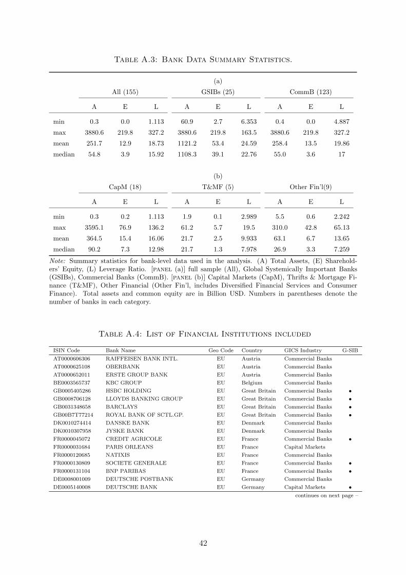
Table A.3: Bank Data Summary Statistics.

(a)

All (155) GSIBs (25) CommB (123)

A E L A E L A E L

min 0.3 0.0 1.113 60.9 2.7 6.353 0.4 0.0 4.887

max 3880.6 219.8 327.2 3880.6 219.8 163.5 3880.6 219.8 327.2

mean 251.7 12.9 18.73 1121.2 53.4 24.59 258.4 13.5 19.86

median 54.8 3.9 15.92 1108.3 39.1 22.76 55.0 3.6 17

(b)

CapM (18) T&MF (5) Other Fin’l(9)

A E L A E L A E L

min 0.3 0.2 1.113 1.9 0.1 2.989 5.5 0.6 2.242

max 3595.1 76.9 136.2 61.2 5.7 19.5 310.0 42.8 65.13

mean 364.5 15.4 16.06 21.7 2.5 9.933 63.1 6.7 13.65

median 90.2 7.3 12.98 21.7 1.3 7.978 26.9 3.3 7.259

Note: Summary statistics for bank-level data used in the analysis. (A) Total Assets, (E) Sharehold-ers’ Equity, (L) Leverage Ratio. [panel (a)] full sample (All), Global Systemically Important Banks(GSIBs), Commercial Banks (CommB). [panel (b)] Capital Markets (CapM), Thrifts & Mortgage Fi-nance (T&MF), Other Financial (Other Fin’l, includes Diversified Financial Services and ConsumerFinance). Total assets and common equity are in Billion USD. Numbers in parentheses denote thenumber of banks in each category.

Table A.4: List of Financial Institutions included

ISIN Code Bank Name Geo Code Country GICS Industry G-SIB

AT0000606306 RAIFFEISEN BANK INTL. EU Austria Commercial Banks

AT0000625108 OBERBANK EU Austria Commercial Banks

AT0000652011 ERSTE GROUP BANK EU Austria Commercial Banks

BE0003565737 KBC GROUP EU Belgium Commercial Banks

GB0005405286 HSBC HOLDING EU Great Britain Commercial Banks •GB0008706128 LLOYDS BANKING GROUP EU Great Britain Commercial Banks •GB0031348658 BARCLAYS EU Great Britain Commercial Banks •GB00B7T77214 ROYAL BANK OF SCTL.GP. EU Great Britain Commercial Banks •DK0010274414 DANSKE BANK EU Denmark Commercial Banks

DK0010307958 JYSKE BANK EU Denmark Commercial Banks

FR0000045072 CREDIT AGRICOLE EU France Commercial Banks •FR0000031684 PARIS ORLEANS EU France Capital Markets

FR0000120685 NATIXIS EU France Commercial Banks

FR0000130809 SOCIETE GENERALE EU France Commercial Banks •FR0000131104 BNP PARIBAS EU France Commercial Banks •DE0008001009 DEUTSCHE POSTBANK EU Germany Commercial Banks

DE0005140008 DEUTSCHE BANK EU Germany Capital Markets •continues on next page –

42

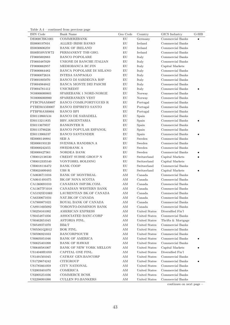
Table A.4 – continued from previous page


DE000CBK1001 COMMERZBANK EU Germany Commercial Banks •IE0000197834 ALLIED IRISH BANKS EU Ireland Commercial Banks

IE0030606259 BANK OF IRELAND EU Ireland Commercial Banks

IE00B59NXW72 PERMANENT TSB GHG. EU Ireland Commercial Banks

IT0005002883 BANCO POPOLARE EU Italy Commercial Banks

IT0003487029 UNIONE DI BANCHE ITALIAN EU Italy Commercial Banks

IT0000062957 MEDIOBANCA BC.FIN EU Italy Capital Markets

IT0000064482 BANCA POPOLARE DI MILANO EU Italy Commercial Banks

IT0000072618 INTESA SANPAOLO EU Italy Commercial Banks

IT0001005070 BANCO DI SARDEGNA RSP EU Italy Commercial Banks

IT0004984842 BANCA MONTE DEI PASCHI EU Italy Commercial Banks

IT0004781412 UNICREDIT EU Italy Commercial Banks •NO0006000801 SPAREBANK 1 NORD-NORGE EU Norway Commercial Banks

NO0006000900 SPAREBANKEN VEST EU Norway Commercial Banks

PTBCP0AM0007 BANCO COMR.PORTUGUES R EU Portugal Commercial Banks

PTBES0AM0007 BANCO ESPIRITO SANTO EU Portugal Commercial Banks

PTBPI0AM0004 BANCO BPI EU Portugal Commercial Banks

ES0113860A34 BANCO DE SABADELL EU Spain Commercial Banks

ES0113211835 BBV.ARGENTARIA EU Spain Commercial Banks •ES0113679I37 BANKINTER R EU Spain Commercial Banks

ES0113790226 BANCO POPULAR ESPANOL EU Spain Commercial Banks

ES0113900J37 BANCO SANTANDER EU Spain Commercial Banks •SE0000148884 SEB A EU Sweden Commercial Banks

SE0000193120 SVENSKA HANDBKN.A EU Sweden Commercial Banks

SE0000242455 SWEDBANK A EU Sweden Commercial Banks

SE0000427361 NORDEA BANK EU Sweden Commercial Banks •CH0012138530 CREDIT SUISSE GROUP N EU Switzerland Capital Markets •CH0012335540 VONTOBEL HOLDING EU Switzerland Capital Markets

CH0018116472 BANK COOP EU Switzerland Commercial Banks

CH0024899483 UBS R EU Switzerland Capital Markets •CA0636711016 BANK OF MONTREAL AM Canada Commercial Banks

CA0641491075 BK.OF NOVA SCOTIA AM Canada Commercial Banks

CA1360691010 CANADIAN IMP.BK.COM. AM Canada Commercial Banks

CA13677F1018 CANADIAN WESTERN BANK AM Canada Commercial Banks

CA51925D1069 LAURENTIAN BK.OF CANADA AM Canada Commercial Banks

CA6330671034 NAT.BK.OF CANADA AM Canada Commercial Banks

CA7800871021 ROYAL BANK OF CANADA AM Canada Commercial Banks

CA8911605092 TORONTO-DOMINION BANK AM Canada Commercial Banks

US0258161092 AMERICAN EXPRESS AM United States Diversified Fin’l

US0454871056 ASSOCIATED BANC-CORP AM United States Commercial Banks

US0462651045 ASTORIA FINL. AM United States Thrifts & Mortgage

US0549371070 BB&T AM United States Commercial Banks

US05561Q2012 BOK FINL. AM United States Commercial Banks

US0596921033 BANCORPSOUTH AM United States Commercial Banks

US0605051046 BANK OF AMERICA AM United States Commercial Banks •US0625401098 BANK OF HAWAII AM United States Commercial Banks

US0640581007 BANK OF NEW YORK MELLON AM United States Capital Markets •US14040H1059 CAPITAL ONE FINL. AM United States Diversified Fin’l

US1491501045 CATHAY GEN.BANCORP AM United States Commercial Banks

US1729674242 CITIGROUP AM United States Commercial Banks •US1785661059 CITY NATIONAL AM United States Commercial Banks

US2003401070 COMERICA AM United States Commercial Banks

US2005251036 COMMERCE BCSH. AM United States Commercial Banks

US2298991090 CULLEN FO.BANKERS AM United States Commercial Banks

continues on next page –

43



US2692464017 E*TRADE FINANCIAL AM United States Capital Markets

US27579R1041 EAST WEST BANCORP AM United States Commercial Banks

US3167731005 FIFTH THIRD BANCORP AM United States Commercial Banks

US31946M1036 FIRST CTZN.BCSH.A AM United States Commercial Banks

US3205171057 FIRST HORIZON NATIONAL AM United States Commercial Banks

US33582V1089 FIRST NIAGARA FINL.GP. AM United States Commercial Banks

US3379151026 FIRSTMERIT AM United States Commercial Banks

US3546131018 FRANKLIN RESOURCES AM United States Capital Markets

US3602711000 FULTON FINANCIAL AM United States Commercial Banks

US38141G1040 GOLDMAN SACHS GP. AM United States Capital Markets •US4436831071 HUDSON CITY BANC. AM United States Thrifts & Mortgage

US4461501045 HUNTINGTON BCSH. AM United States Commercial Banks

US4508281080 IBERIABANK AM United States Commercial Banks

US4590441030 INTERNATIONAL BCSH. AM United States Commercial Banks

US46625H1005 JP MORGAN CHASE & CO. AM United States Commercial Banks •US4932671088 KEYCORP AM United States Commercial Banks

US55261F1049 M&T BANK AM United States Commercial Banks

US55264U1088 MB FINANCIAL AM United States Commercial Banks

US6174464486 MORGAN STANLEY AM United States Capital Markets •US6494451031 NEW YORK COMMUNITY BANC. AM United States Thrifts & Mortgage

US6658591044 NORTHERN TRUST AM United States Capital Markets

US6934751057 PNC FINL.SVS.GP. AM United States Commercial Banks

US7127041058 PEOPLES UNITED FINANCIAL AM United States Thrifts & Mortgage

US7429621037 PRIVATEBANCORP AM United States Commercial Banks

US7547301090 RAYMOND JAMES FINL. AM United States Capital Markets

US7591EP1005 REGIONS FINL.NEW AM United States Commercial Banks

US78442P1066 SLM AM United States Diversified Fin’l

US78486Q1013 SVB FINANCIAL GROUP AM United States Commercial Banks

US8085131055 CHARLES SCHWAB AM United States Capital Markets

US8574771031 STATE STREET AM United States Capital Markets •US8679141031 SUNTRUST BANKS AM United States Commercial Banks

US8690991018 SUSQUEHANNA BCSH. AM United States Commercial Banks

US87161C5013 SYNOVUS FINANCIAL AM United States Commercial Banks

US8722751026 TCF FINANCIAL AM United States Commercial Banks

US87236Y1082 TD AMERITRADE HOLDING AM United States Capital Markets

US9027881088 UMB FINANCIAL AM United States Commercial Banks

US9029733048 US BANCORP AM United States Commercial Banks

US9042141039 UMPQUA HOLDINGS AM United States Commercial Banks

US9197941076 VALLEY NATIONAL BANCORP AM United States Commercial Banks

US9388241096 WASHINGTON FEDERAL AM United States Thrifts & Mortgage

US9478901096 WEBSTER FINANCIAL AM United States Commercial Banks

US9497461015 WELLS FARGO & CO AM United States Commercial Banks •US97650W1080 WINTRUST FINANCIAL AM United States Commercial Banks

US9897011071 ZIONS BANCORP. AM United States Commercial Banks

JP3902900004 MITSUBISHI UFJ FINL.GP. AS Japan Commercial Banks •JP3890350006 SUMITOMO MITSUI FINL.GP. AS Japan Commercial Banks •JP3429200003 SHINKIN CENTRAL BANK PF. AS Japan Commercial Banks

JP3805010000 FUKUOKA FINANCIAL GP. AS Japan Commercial Banks

JP3842400008 HOKUHOKU FINL. GP. AS Japan Commercial Banks

JP3105040004 AIFUL AS Japan Diversified Fin’l

JP3107600003 AKITA BANK AS Japan Commercial Banks

JP3108600002 ACOM AS Japan Diversified Fin’l

JP3152400002 BANK OF IWATE AS Japan Commercial Banks

JP3175200009 OITA BANK AS Japan Commercial Banks

continues on next page –

44



JP3194600007 BANK OF OKINAWA AS Japan Commercial Banks

JP3200450009 ORIX AS Japan Diversified Fin’l

JP3207800008 KAGOSHIMA BANK AS Japan Commercial Banks

JP3271400008 CREDIT SAISON AS Japan Diversified Fin’l

JP3276400003 GUNMA BANK AS Japan Commercial Banks

JP3351200005 SHIZUOKA BANK AS Japan Commercial Banks

JP3352000008 77 BANK AS Japan Commercial Banks

JP3388600003 JACCS AS Japan Diversified Fin’l

JP3392200006 EIGHTEENTH BANK AS Japan Commercial Banks

JP3392600007 JUROKU BANK AS Japan Commercial Banks

JP3394200004 JOYO BANK AS Japan Commercial Banks

JP3441600008 TAIKO BANK AS Japan Commercial Banks

JP3502200003 DAIWA SECURITIES GROUP AS Japan Capital Markets

JP3511800009 CHIBA BANK AS Japan Commercial Banks

JP3520000005 CHUKYO BANK AS Japan Commercial Banks

JP3521000004 CHUGOKU BANK AS Japan Commercial Banks

JP3587000005 TOKYO TOMIN BANK AS Japan Commercial Banks

JP3601000007 TOHO BANK AS Japan Commercial Banks

JP3630500001 TOMATO BANK AS Japan Commercial Banks

JP3653400006 NANTO BANK AS Japan Commercial Banks

JP3762600009 NOMURA HDG. AS Japan Capital Markets

JP3769000005 HACHIJUNI BANK AS Japan Commercial Banks

JP3783800000 HIGO BANK AS Japan Commercial Banks

JP3786600001 HITACHI CAPITAL AS Japan Diversified Fin’l

JP3841000007 HOKUETSU BANK AS Japan Commercial Banks

JP3881200004 MIE BANK AS Japan Commercial Banks

JP3888000001 MICHINOKU BANK AS Japan Commercial Banks

JP3905850008 MINATO BANK AS Japan Commercial Banks

JP3942000005 YAMANASHI CHUO BK. AS Japan Commercial Banks

JP3955400001 BANK OF YOKOHAMA AS Japan Commercial Banks

Notes: In the first column are the ISIN identification codes followed by the institution’s name, ge-

ographical location and country of reference. The last column highlights the subset of institutions

which have been classified as Global Systemically Important Banks (G-SIBs) previously known as

G-SIFIs (Systemically Important Financial Institutions); the classification has been adopted by the

Financial Stability Board starting from November 2011 and lastly updated in November 2013.

45

Figure A.3: Quarterly asset growth over quarterly leverage growthacross different global financial institutions

−20 −10 0 10 20−10

−5

0

5

10

15

20

Q2−03

Q3−03

Q4−03

Q1−04

Q2−04Q3−04Q4−04

Q1−05

Q2−05

Q3−05

Q4−05

Q1−06

Q2−06Q3−06

Q4−06

Q1−07

Q2−07Q3−07

Q4−07

Q1−08

Q2−08

Q3−08

Q4−08

Q1−09

Q2−09

Q3−09

Q4−09

Q1−10

Q2−10Q3−10

Q4−10

Q1−11

Q2−11Q3−11 Q4−11

Q1−12

Q2−12

Q3−12

Q4−12

Q1−13Q2−13Q3−13

Q4−13

Q1−14

Q2−14

G−SIBs (25)

Qu

art

erly

Ass

et G

row

th

−20 −15 −10 −5 0 5 10−10

−5

0

5

10

15

Q2−03

Q3−03

Q4−03

Q1−04

Q2−04 Q3−04Q4−04

Q1−05

Q2−05

Q3−05

Q4−05

Q1−06

Q2−06

Q3−06

Q4−06

Q1−07

Q2−07

Q3−07

Q4−07

Q1−08

Q2−08Q3−08

Q4−08

Q1−09

Q2−09

Q3−09

Q4−09

Q1−10

Q2−10Q3−10

Q4−10

Q1−11

Q2−11Q3−11

Q4−11Q1−12

Q2−12

Q3−12

Q4−12

Q1−13Q2−13Q3−13

Q4−13

Q1−14

Q2−14

Commercial Banks (122)

−20 −10 0 10 20 30 40−10

−5

0

5

10

15

20

25

30

Q2−03Q3−03

Q4−03

Q1−04

Q2−04

Q3−04Q4−04

Q1−05

Q2−05 Q3−05Q4−05Q1−06

Q2−06Q3−06

Q4−06Q1−07

Q2−07

Q3−07Q4−07Q1−08

Q2−08

Q3−08

Q4−08Q1−09

Q2−09

Q3−09

Q4−09

Q1−10

Q2−10Q3−10Q4−10

Q1−11

Q2−11Q3−11

Q4−11

Q1−12

Q2−12Q3−12Q4−12

Q1−13Q2−13Q3−13

Q4−13Q1−14

Q2−14

Capital Markets (18)

−10 −5 0 5 10 15 20−10

−5

0

5

10

15

20

Q2−03Q3−03

Q4−03

Q1−04

Q2−04

Q3−04Q4−04

Q1−05

Q2−05

Q3−05

Q4−05

Q1−06

Q2−06Q3−06 Q4−06

Q1−07

Q2−07Q3−07

Q4−07Q1−08Q2−08

Q3−08Q4−08

Q1−09

Q2−09Q3−09

Q4−09

Q1−10

Q2−10

Q3−10Q4−10Q1−11

Q2−11

Q3−11Q4−11Q1−12

Q2−12

Q3−12Q4−12Q1−13Q2−13Q3−13

Q4−13 Q1−14Q2−14

Other Financial (14)

Quarterly Leverage Growth

Note: he red line in each subplot is the 45 degree line. Clockwise, from top left panel, the relationshipbetween balance sheet size and leverage for GISBs, commercial banks, institutions operating in capitalmarkets and other financial institutions. The classification matches GICS industry codes for each entryin the sample. Source: Datastream, authors calculations.

46

B Dynamic Factor Model for World Risky Asset Prices

– For Online Publication

Let pt be an n-dimensional vector collecting monthly (log) asset price series pi,t, where

pi,t denotes the price for asset i at date t. We assume

pt = ΛFt + ξt . (B.1)

Ft is an (r × 1) vector of common factors (Ft = [f1,t, . . . , fr,t]′) that capture systematic

sources of variation among prices and are loaded via the coefficients in Λ that determine

how each price series reacts to the common shocks. ξt is a (n × 1) vector of idiosyn-

cratic shocks ξi,t that capture series-specific variability or measurement errors. We allow

elements in ξt to display some degree of autocorrelation while we rule out pairwise corre-

lation between assets assuming that all the co-variation is accounted for by the common

component. Both the common factors and the idiosyncratic terms are assumed to be zero

mean processes.

The factors are assumed to follow a VAR process of order p

Ft = Φ1Ft−1 + . . .+ ΦpFt−p + εt, (B.2)

where the autoregressive coefficients are collected in the p matrices Φ1, . . . ,Φp, each of

which is (r×r); the error term εt is a normally distributed zero mean process with covari-

ance matrix Q. Any residual autocorrelation is captured by the idiosyncratic component

which we assume being a collection of independent univariate autoregressive processes.

In order to distinguish between comovements at different levels of aggregation we

model asset prices such that each series is a function of a global factor, a regional factor

and an idiosyncratic term. We do so by allowing the vector of common shocks to include

both aggregate shocks that affect all series in yt, and shocks that affect many but not all

of them:

pi,t = λi,gfgt + λi,mf

mt + ξi,t . (B.3)

In Eq. (B.3) the common component ΛFt is separated into a global factor (f gt ) and a

regional or market-specific factor (fmt ) which is meant to capture commonalities among

many but not all price series. Each pi,t is thus a function of a global factor loaded by

all the variables in pt, a regional or market-specific factor only loaded by those series in

pt that belong to the (geographical or sector-specific) market m, and of a series-specific

factor.

Such hierarchical structure is imposed via zero restrictions on some of the elements in

47

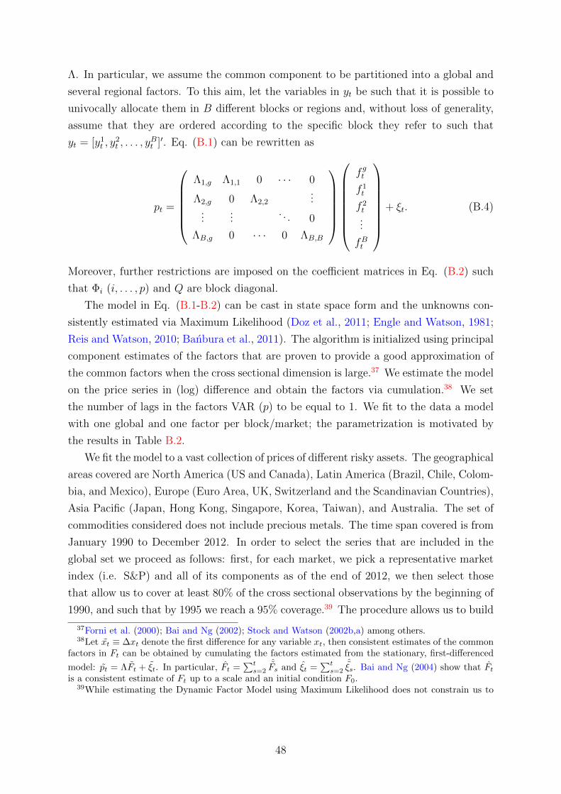
Λ. In particular, we assume the common component to be partitioned into a global and

several regional factors. To this aim, let the variables in yt be such that it is possible to

univocally allocate them in B different blocks or regions and, without loss of generality,

assume that they are ordered according to the specific block they refer to such that

yt = [y1t , y

2t , . . . , y

Bt ]′. Eq. (B.1) can be rewritten as

pt =

Λ1,g Λ1,1 0 · · · 0

Λ2,g 0 Λ2,2...

......

. . . 0

ΛB,g 0 · · · 0 ΛB,B

f gt

f 1t

f 2t...

fBt

+ ξt. (B.4)

Moreover, further restrictions are imposed on the coefficient matrices in Eq. (B.2) such

that Φi (i, . . . , p) and Q are block diagonal.

The model in Eq. (B.1-B.2) can be cast in state space form and the unknowns con-

sistently estimated via Maximum Likelihood (Doz et al., 2011; Engle and Watson, 1981;

Reis and Watson, 2010; Banbura et al., 2011). The algorithm is initialized using principal

component estimates of the factors that are proven to provide a good approximation of

the common factors when the cross sectional dimension is large.37 We estimate the model

on the price series in (log) difference and obtain the factors via cumulation.38 We set

the number of lags in the factors VAR (p) to be equal to 1. We fit to the data a model

with one global and one factor per block/market; the parametrization is motivated by

the results in Table B.2.

We fit the model to a vast collection of prices of different risky assets. The geographical

areas covered are North America (US and Canada), Latin America (Brazil, Chile, Colom-

bia, and Mexico), Europe (Euro Area, UK, Switzerland and the Scandinavian Countries),

Asia Pacific (Japan, Hong Kong, Singapore, Korea, Taiwan), and Australia. The set of

commodities considered does not include precious metals. The time span covered is from

January 1990 to December 2012. In order to select the series that are included in the

global set we proceed as follows: first, for each market, we pick a representative market

index (i.e. S&P) and all of its components as of the end of 2012, we then select those

that allow us to cover at least 80% of the cross sectional observations by the beginning of

1990, and such that by 1995 we reach a 95% coverage.39 The procedure allows us to build

37Forni et al. (2000); Bai and Ng (2002); Stock and Watson (2002b,a) among others.38Let xt ≡ ∆xt denote the first difference for any variable xt, then consistent estimates of the common

factors in Ft can be obtained by cumulating the factors estimated from the stationary, first-differenced

model: pt = ΛFt + ξt. In particular, Ft =∑t

s=2ˆFs and ξt =

∑ts=2

ˆξs. Bai and Ng (2004) show that Ft

is a consistent estimate of Ft up to a scale and an initial condition F0.39While estimating the Dynamic Factor Model using Maximum Likelihood does not constrain us to

48

Table B.1: Composition of asset price panels

North America Latin America Europe Asia Pacific Australia Cmdy Corporate Total

1975:2010 114 – 82 68 – 39 – 303

1990:2012 364 16 200 143 21 57 57 858

Note: Composition of the panels of asset prices used for the estimation of the global factor. Columnsdenote blocks/markets in each set, while the number in each cell corresponds to the number of elementsin each block.

a final dataset with an overall cross-sectional dimension of n = 858. The composition is

reported in Table B.1, where each category (in columns) corresponds to one of the blocks

(m) within the structure imposed.

Although all series included in the set are priced in US dollars, we verify that the

shape of the global factor is not influenced by this choice by estimating the same model

on price series in their local currencies (i.e. the currency in which the assets are originally

traded). The resulting global factor (not shown) is very similar to the one constructed

from the dollar-denominated set both in terms of overall shape and of peaks and troughs

that perfectly coincide throughout the time span considered. Intuitively, the robustness of

the estimate of the global factor with respect to currency transformations comes directly

from the structure imposed in Eq. (B.3). The blocks/markets structure imposed roughly

coincides with currency areas, therefore this aspect is likely to be largely captured by the

regional factors (see Table B.1).

B.1 The Number of Factors

To choose the number of global factors we use a number of criteria and tests, collected

in Table B.2. The table reports the percentage of variance that is explained by the i-th

eigenvalue (in decreasing order) of both the covariance matrix and the spectral density

matrix, the information criteria in Bai and Ng (2002), where the residual variance of the

idiosyncratic component is minimized subject to a penalty function increasing in r, and

the test developed in Onatski (2009), where the null of r − 1 factors is tested against

the alternative of r common factors. The largest eigenvalue alone, in both the time and

frequency domain, accounts for about 60% of the variability in the data in the longer set

and about a fourth of the variation in the shorter, but more heterogeneous set; similarly,

the IC criteria reach their minimum when one factor is used, and the overall picture is

confirmed by the the p-values for the Onatski test.

work with a fully balanced panel, we want to ensure that none of the categories included in the set isoverrepresented at any point in time.

49

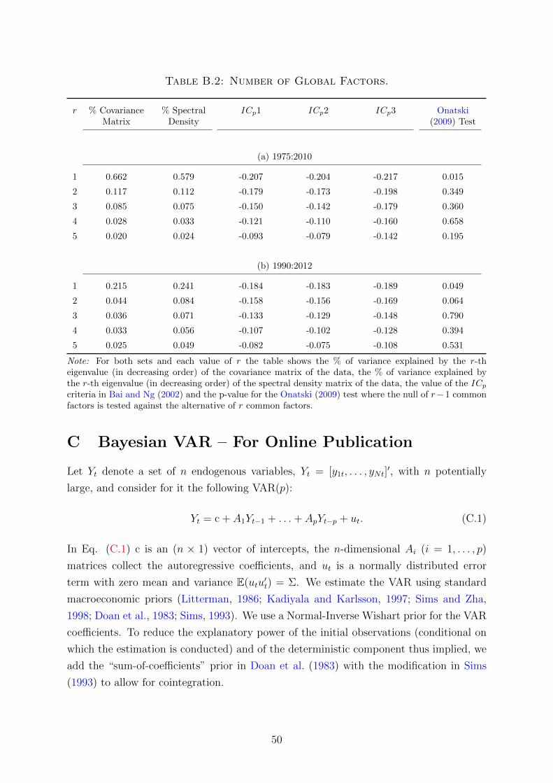
Table B.2: Number of Global Factors.

r % CovarianceMatrix

% SpectralDensity

ICp1 ICp2 ICp3 Onatski(2009) Test

(a) 1975:2010

1 0.662 0.579 -0.207 -0.204 -0.217 0.015

2 0.117 0.112 -0.179 -0.173 -0.198 0.349

3 0.085 0.075 -0.150 -0.142 -0.179 0.360

4 0.028 0.033 -0.121 -0.110 -0.160 0.658

5 0.020 0.024 -0.093 -0.079 -0.142 0.195

(b) 1990:2012

1 0.215 0.241 -0.184 -0.183 -0.189 0.049

2 0.044 0.084 -0.158 -0.156 -0.169 0.064

3 0.036 0.071 -0.133 -0.129 -0.148 0.790

4 0.033 0.056 -0.107 -0.102 -0.128 0.394

5 0.025 0.049 -0.082 -0.075 -0.108 0.531

Note: For both sets and each value of r the table shows the % of variance explained by the r-theigenvalue (in decreasing order) of the covariance matrix of the data, the % of variance explained bythe r-th eigenvalue (in decreasing order) of the spectral density matrix of the data, the value of the ICp

criteria in Bai and Ng (2002) and the p-value for the Onatski (2009) test where the null of r−1 commonfactors is tested against the alternative of r common factors.

C Bayesian VAR – For Online Publication

Let Yt denote a set of n endogenous variables, Yt = [y1t, . . . , yNt]′, with n potentially

large, and consider for it the following VAR(p):

Yt = c + A1Yt−1 + . . .+ ApYt−p + ut. (C.1)

In Eq. (C.1) c is an (n × 1) vector of intercepts, the n-dimensional Ai (i = 1, . . . , p)

matrices collect the autoregressive coefficients, and ut is a normally distributed error

term with zero mean and variance E(utu′t) = Σ. We estimate the VAR using standard

macroeconomic priors (Litterman, 1986; Kadiyala and Karlsson, 1997; Sims and Zha,

1998; Doan et al., 1983; Sims, 1993). We use a Normal-Inverse Wishart prior for the VAR

coefficients. To reduce the explanatory power of the initial observations (conditional on

which the estimation is conducted) and of the deterministic component thus implied, we

add the “sum-of-coefficients” prior in Doan et al. (1983) with the modification in Sims

(1993) to allow for cointegration.

50

The Normal-Inverse Wishart prior takes the following form:

Σ ∼ W−1(Ψ, ν) (C.2)

β|Σ ∼ N (b,Σ⊗ Ω) (C.3)

where β is a vector collecting all the VAR parameters, i.e. β ≡ vec([c, A1, . . . , Ap]′). The

degrees of freedom of the Inverse-Wishart are set such that the mean of the distribution

exists and are equal to ν = n+ 2, Ψ is diagonal with elements ψi which are chosen to be

a function of the residual variance of the regression of each variable onto its own first p

lags. More specifically, the parameters in Eq. (C.2) and Eq. (C.3) are chosen to match

the moments for the distribution of the coefficients in Eq. (C.1) defined by the Minnesota

priors:

E[(Ai)jk] =

δj i = 1, j = k

0 otherwiseVar[(Ai)jk] =

λ2

i2j = k

λ2

i2σ2k

σ2j

otherwise,(C.4)

where (Ai)jk denotes the element in row (equation) j and column (variable) k of the

coefficients matrix A at lag i (i = 1, . . . , p). When δj = 1 the random walk prior is

strictly imposed on all variables; however, for those variables for which this prior is not

suitable we set δj = 0 as in Banbura et al. (2010). On the right hand side of Eq. (C.4),

the variance of the elements in Ai is assumed to be proportional to the (inverse of the)

square of the lag (i2), and to the relative variance of the variables.

The priors are implemented via the addition of dummy observations in the spirit

of Theil and Goldberger (1961). Let γ ≡ [λ, µ, τ ]′ be the vector of hyperparameters

controlling the overall tightness of the priors. We use λ for the Normal-Inverse Wishart

prior, µ for the sum-of-coefficients prior, and τ for the cointegration prior. We follow

Giannone et al. (2015) and treat the γ as an additional model parameter which we

estimate in the spirit of hierarchical modelling.

D Proxy SVAR and Narrative Instrument – For On-

line Publication

D.1 Identification with External Instruments

Let the structural representation of Eq. (C.1) be

B−10 Yt = c +B1Yt−1 + . . .+BpYt−p + et, (D.1)

51

Table C.1: variance decomposition: selected variables

0 1 4 8 12 16 20

USGDP 0 0.02 4.41 11.54 16.81 17.27 16.02

GDPDEF 0 0.02 0.05 0.33 1.38 2.55 3.43

GDC 0 0.12 0.58 0.95 1.91 3.56 5.62

FEDFUNDS 74.39 67.29 48.71 29.74 20.58 17.14 15.99

GCB 3.03 4.44 5.06 5.54 8.90 12.40 14.01

GCNB 3.49 3.88 3.20 1.85 1.38 1.65 2.47

BDLEV 0.30 0.91 2.16 1.91 1.75 1.63 1.62

EURLEVQ 0.24 1.35 3.31 2.94 2.65 2.54 2.69

GBPLEVQ 0.00 0.94 2.36 3.04 2.72 2.57 2.58

GFAC 0.55 1.45 1.01 1.22 2.14 2.18 2.08

Note: The table reports the forecast error variance decomposition (% points) in the baseline BVAR(4), forthe variables listed in Table 1 under the recursive identification. Relevant forecast horizons in columns.

where the reduced-form autoregressive coefficients are such that Ai = B0Bi, i = 1, . . . , n,

and the VAR innovations

ut = B0et. (D.2)

We estimate the relevant entries of B0 using an external instrument zt that is assumed

to be correlated with the structural shocks of interest but uncorrelated with all other

structural shocks (Mertens and Ravn, 2013; Stock and Watson, 2012).

The identifying assumptions are

E(zte′1,t) = κ E(zte

′2,t) = 0, (D.3)

where e1,t is the shock of interest (e.g. monetary policy shock in our case) and e2,t contains

all the other shocks. Let Sxy denote E(xty′t) and partition B0 such that:

B0 =

[b11 b12

b21 b22

],

then conditions in Eq. (D.2) and (D.3) imply that

b21b−111 = S−1

zu′1Szu′2 . (D.4)

Eq. (D.4) establishes that the ratio b21b−111 can be estimated using only moments of

observables; in particular, the estimate of S−1zu′1

Szu′2 corresponds to the two stages least

square estimator in a regression of u2,t on u1,t, where zt is used as an instrument for u1,t.

52

Figure D.1: Narrative Instrument

1969 1974 1979 1984 1989 1994 1999 2004−10

−8

−6

−4

−2

0

2

4

6

8

Actual Change in FFRNarrative Instrument

Note: Narrative-based instrument for monetary policy shock in the US (light blue line) versus actualchanges in the Federal Fund Rates (blue dotted line) over the same sample.

D.2 Narrative Instrument

We construct our external instrument by extending the narrative series first proposed in

Romer and Romer (2004) (RR04 henceforth) until the end of 2007. The original series

covered the period 1969-1996.

The narrative-based instrument for the monetary policy shock is constructed as the

residual of the following regression (Eq. (1) in RR04):

∆FFRm =α + βFFRm + ρu(m)t+0|t

+2∑

j=−1

γjy(m)t+j|t +

2∑j=−1

λj

[y

(m)t+j|t − y

(m−1)t+j|t

]+

2∑j=−1

φj∆π(m)t+j|t +

2∑j=−1

θj

[∆π

(m)t+j|t −∆π

(m−1)t+j|t

]+ εm. (D.5)

Eq. (D.5) is estimated at FOMC meeting dates (indexed by m). ∆FFRm is the change

in the intended funds rate around the FOMC meeting while FFRm is the level of the

rate before any change associated to the meeting m takes place. u, y and π are used

to denote the unemployment rate, real output growth and inflation respectively, while

the notation t+ j|t denotes forecasts for quarter t+ j where t is the quarter the specific

FOMC meeting m belongs to, such that y(m)t+1|t denotes the forecast for real output growth

(y), relative to the next quarter (t+ 1|t), which is available at meeting m.

At the time of the construction of the instrument (February 2014) Greenbook forecasts

53

were available only up to the end of 2007, hence our sample ends at this date. Data relative

to the fed funds rate level at each FOMC meeting date for the subperiod 1997-2007 are

from Bloomberg. Following RR04, we obtain our quarterly instrument by summing up

the residuals of Eq. (D.5) over the observations relative to the meeting dates belonging

to each specific quarter. The variable is plotted in Figure D.1 against the actual changes

in the federal funds rate.

54

E Other Charts – For Online Publication

55

Figure E.1: full set of responses - baseline set

USGDP

0 4 8 12 16 20

−8

−6

−4

−2

0

EUGDP

0 4 8 12 16 20

−0.4

−0.2

0

0.2

0.4IPROD

0 4 8 12 16 20

−6

−4

−2

0

2RPCE

0 4 8 12 16 20

−8

−6

−4

−2

0

RPFINR

0 4 8 12 16 20

−10

−5

0

5

RPFIR

0 4 8 12 16 20

−20

−10

0

EMPLY

0 4 8 12 16 20−5

−4

−3

−2

−1

0

CSENT

0 4 8 12 16 20−4

−3

−2

−1

0

1

GDPDEF

0 4 8 12 16 20

−6

−4

−2

0

PCEDEF

0 4 8 12 16 20

−6

−4

−2

0

GDC

0 4 8 12 16 20

−20

−10

0

FEDFUNDS

0 4 8 12 16 20

0

0.5

1

GCB

0 4 8 12 16 20

−30

−20

−10

0

GCNB

0 4 8 12 16 20−30

−20

−10

0

BDLEV

0 4 8 12 16 20−3

−2

−1

0

1

2EURLEVQ

0 4 8 12 16 20

−0.6

−0.4

−0.2

0

0.2

0.4

GBPLEVQ

0 4 8 12 16 20

−0.5

0

0.5

USDEUR

0 4 8 12 16 20

−10

−5

0

5

10

USDGBP

0 4 8 12 16 20

−5

0

5

10

15

TSPREAD

0 4 8 12 16 20−0.6

−0.4

−0.2

0

0.2

EURATE

0 4 8 12 16 20

−0.2

0

0.2

0.4

UKRATE

0 4 8 12 16 20

−0.4

−0.2

0

0.2

0.4

0.6

GRVAR

0 4 8 12 16 20

−0.4

−0.2

0

0.2

GFAC

0 4 8 12 16 20

−5

0

5

GZEBP

0 4 8 12 16 20

−0.1

0

0.1

CholeskyNarrative


56

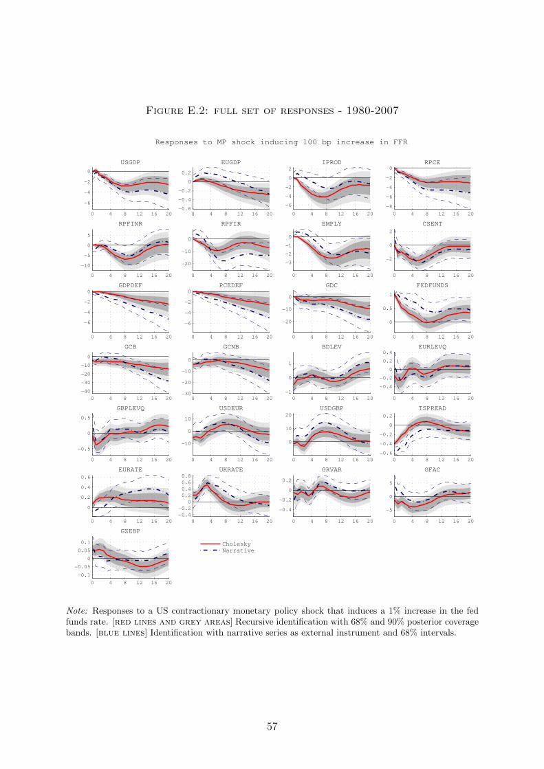
Figure E.2: full set of responses - 1980-2007

Responses to MP shock inducing 100 bp increase in FFR

CholeskyNarrative

GZEBP

0 4 8 12 16 20

−0.1

−0.05

0

0.05

0.1

GFAC

0 4 8 12 16 20

−5

0

5

GRVAR

0 4 8 12 16 20

−0.4

−0.2

0

0.2

UKRATE

0 4 8 12 16 20−0.4−0.2

00.20.40.60.8

EURATE

0 4 8 12 16 20

0

0.2

0.4

0.6

TSPREAD

0 4 8 12 16 20−0.6

−0.4

−0.2

0

0.2

USDGBP

0 4 8 12 16 20

0

10

20USDEUR

0 4 8 12 16 20

−10

0

10

GBPLEVQ

0 4 8 12 16 20

−0.5

0

0.5

EURLEVQ

0 4 8 12 16 20

−0.4

−0.2

0

0.2

0.4BDLEV

0 4 8 12 16 20−1

0

1

GCNB

0 4 8 12 16 20−30

−20

−10

0

GCB

0 4 8 12 16 20

−40

−30

−20

−10

0

FEDFUNDS

0 4 8 12 16 20

0

0.5

1

GDC

0 4 8 12 16 20

−20

−10

0

PCEDEF

0 4 8 12 16 20

−6

−4

−2

0GDPDEF

0 4 8 12 16 20

−6

−4

−2

0

CSENT

0 4 8 12 16 20

−2

0

2

EMPLY

0 4 8 12 16 20

−3

−2

−1

0

RPFIR

0 4 8 12 16 20

−20

−10

0

RPFINR

0 4 8 12 16 20

−10

−5

0

5

RPCE

0 4 8 12 16 20

−8

−6

−4

−2

0IPROD

0 4 8 12 16 20

−6

−4

−2

0

2EUGDP

0 4 8 12 16 20−0.6

−0.4

−0.2

0

0.2

USGDP

0 4 8 12 16 20

−6

−4

−2

0


57

Figure E.3: full set of responses - credit split


CholeskyNarrative

GZEBP

0 4 8 12 16 20

−0.1

0

0.1

GFAC

0 4 8 12 16 20

−5

0

5

GRVAR

0 4 8 12 16 20

−0.4

−0.2

0

0.2

UKRATE

0 4 8 12 16 20

−0.5

0

0.5

EURATE

0 4 8 12 16 20

−0.2

0

0.2

0.4

TSPREAD

0 4 8 12 16 20

−0.4

−0.2

0

0.2

USDGBP

0 4 8 12 16 20−10

0

10

USDEUR

0 4 8 12 16 20

−10

0

10

GBPLEVQ

0 4 8 12 16 20

−0.5

0

0.5

EURLEVQ

0 4 8 12 16 20−0.4

−0.2

0

0.2

0.4

BDLEV

0 4 8 12 16 20

−2

0

2

GCNB

0 4 8 12 16 20−30

−20

−10

0

GCB

0 4 8 12 16 20

−30

−20

−10

0

USDC

0 4 8 12 16 20

−15

−10

−5

0

FEDFUNDS

0 4 8 12 16 20

0

0.5

1

GDCEXUS

0 4 8 12 16 20

−20

−10

0

PCEDEF

0 4 8 12 16 20

−6

−4

−2

0

GDPDEF

0 4 8 12 16 20

−6

−4

−2

0

CSENT

0 4 8 12 16 20

−3

−2

−1

0

1

EMPLY

0 4 8 12 16 20

−3

−2

−1

0

RPFIR

0 4 8 12 16 20

−20

−10

0

RPFINR

0 4 8 12 16 20

−5

0

5

RPCE

0 4 8 12 16 20

−6

−4

−2

0

IPROD

0 4 8 12 16 20

−4

−2

0

2

EUGDP

0 4 8 12 16 20

−0.6

−0.4

−0.2

0

0.2

USGDP

0 4 8 12 16 20

−6

−4

−2

0


58

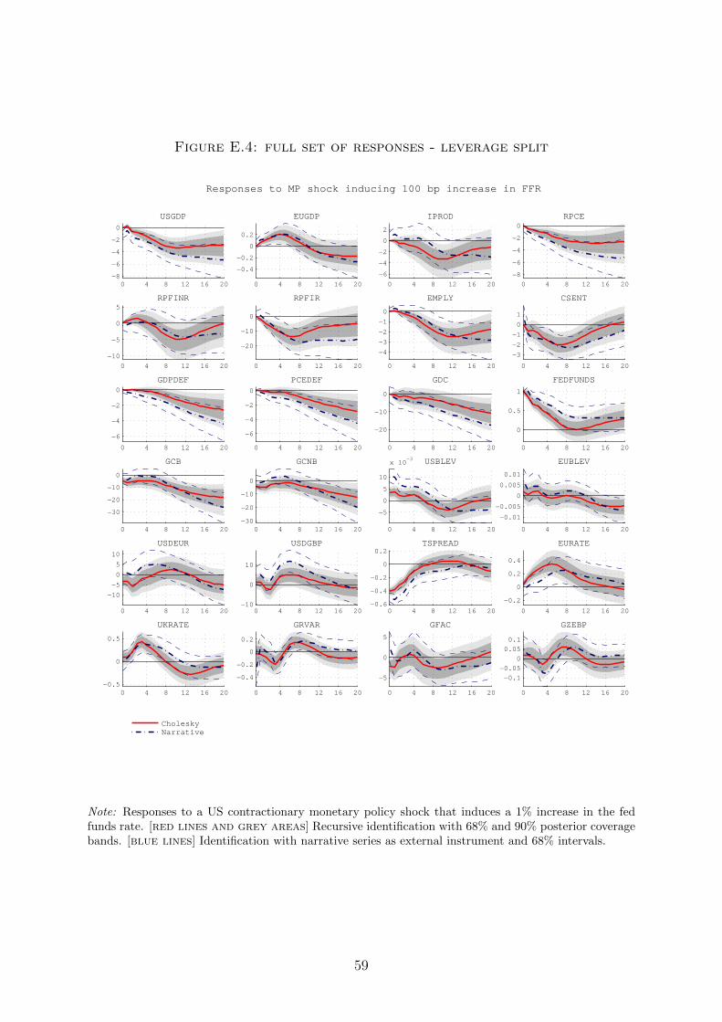
Figure E.4: full set of responses - leverage split


CholeskyNarrative

GZEBP

0 4 8 12 16 20

−0.1

−0.05

0

0.05

0.1

GFAC

0 4 8 12 16 20

−5

0

5

GRVAR

0 4 8 12 16 20

−0.4

−0.2

0

0.2

UKRATE

0 4 8 12 16 20−0.5

0

0.5

EURATE

0 4 8 12 16 20

−0.2

0

0.2

0.4

TSPREAD

0 4 8 12 16 20−0.6

−0.4

−0.2

0

0.2USDGBP

0 4 8 12 16 20−10

0

10

USDEUR

0 4 8 12 16 20

−10

−5

0

5

10

EUBLEV

0 4 8 12 16 20

−0.01

−0.005

0

0.005

0.01

USBLEV

0 4 8 12 16 20

−5

0

5

10

x 10−3GCNB

0 4 8 12 16 20−30

−20

−10

0

GCB

0 4 8 12 16 20

−30

−20

−10

0

FEDFUNDS

0 4 8 12 16 20

0

0.5

1

GDC

0 4 8 12 16 20

−20

−10

0

PCEDEF

0 4 8 12 16 20

−6

−4

−2

0

GDPDEF

0 4 8 12 16 20

−6

−4

−2

0

CSENT

0 4 8 12 16 20

−3

−2

−1

0

1

EMPLY

0 4 8 12 16 20

−4

−3

−2

−1

0

RPFIR

0 4 8 12 16 20

−20

−10

0

RPFINR

0 4 8 12 16 20

−10

−5

0

5

RPCE

0 4 8 12 16 20

−8

−6

−4

−2

0IPROD

0 4 8 12 16 20

−6

−4

−2

0

2

EUGDP

0 4 8 12 16 20

−0.4

−0.2

0

0.2

USGDP

0 4 8 12 16 20−8

−6

−4

−2

0


59

Figure E.5: full set of responses - mp1 instrument


CholeskyMedian MP1

GZEBP

0 4 8 12 16 20

−0.1

−0.05

0

0.05

0.1

GFAC

0 4 8 12 16 20

−5

0

5GRVAR

0 4 8 12 16 20

−0.4

−0.2

0

0.2

UKRATE

0 4 8 12 16 20

−0.4−0.2

00.20.40.6

EURATE

0 4 8 12 16 20

−0.2

0

0.2

0.4

TSPREAD

0 4 8 12 16 20

−0.4

−0.2

0

0.2USDGBP

0 4 8 12 16 20

−5

0

5

10

USDEUR

0 4 8 12 16 20

−10

−5

0

5

10

GBPLEVQ

0 4 8 12 16 20

−0.5

0

0.5

EURLEVQ

0 4 8 12 16 20−0.6

−0.4

−0.2

0

0.2

0.4BDLEV

0 4 8 12 16 20

−2

−1

0

1

GCNB

0 4 8 12 16 20

−20

−10

0

GCB

0 4 8 12 16 20−30

−20

−10

0

FEDFUNDS

0 4 8 12 16 20

0

0.5

1

GDC

0 4 8 12 16 20

−20

−15

−10

−5

0

PCEDEF

0 4 8 12 16 20

−4

−2

0

GDPDEF

0 4 8 12 16 20

−4

−3

−2

−1

0

CSENT

0 4 8 12 16 20

−3

−2

−1

0

1

EMPLY

0 4 8 12 16 20

−4

−3

−2

−1

0

RPFIR

0 4 8 12 16 20

−20

−10

0

RPFINR

0 4 8 12 16 20

−10

−5

0

5

RPCE

0 4 8 12 16 20

−6

−4

−2

0IPROD

0 4 8 12 16 20

−6

−4

−2

0

2EUGDP

0 4 8 12 16 20

−0.4

−0.2

0

0.2

USGDP

0 4 8 12 16 20

−6

−4

−2

0


60

Figure E.6: full set of responses - Target Factor instrument


CholeskyMedian Target

GZEBP

0 4 8 12 16 20

−0.1

−0.05

0

0.05

0.1

GFAC

0 4 8 12 16 20

−5

0

5GRVAR

0 4 8 12 16 20

−0.4

−0.2

0

0.2

UKRATE

0 4 8 12 16 20

−0.4−0.2

00.20.40.6

EURATE

0 4 8 12 16 20

−0.2

0

0.2

0.4

TSPREAD

0 4 8 12 16 20

−0.4

−0.2

0

0.2USDGBP

0 4 8 12 16 20

−5

0

5

10

USDEUR

0 4 8 12 16 20

−10

−5

0

5

10

GBPLEVQ

0 4 8 12 16 20

−0.5

0

0.5

EURLEVQ

0 4 8 12 16 20−0.6

−0.4

−0.2

0

0.2

0.4BDLEV

0 4 8 12 16 20

−2

−1

0

1

GCNB

0 4 8 12 16 20

−20

−10

0

GCB

0 4 8 12 16 20−30

−20

−10

0

FEDFUNDS

0 4 8 12 16 20

0

0.5

1

GDC

0 4 8 12 16 20

−20

−15

−10

−5

0

PCEDEF

0 4 8 12 16 20

−4

−2

0

GDPDEF

0 4 8 12 16 20

−4

−3

−2

−1

0

CSENT

0 4 8 12 16 20

−3

−2

−1

0

1

EMPLY

0 4 8 12 16 20

−4

−3

−2

−1

0

RPFIR

0 4 8 12 16 20

−20

−10

0

RPFINR

0 4 8 12 16 20

−10

−5

0

5

RPCE

0 4 8 12 16 20

−6

−4

−2

0IPROD

0 4 8 12 16 20

−6

−4

−2

0

2EUGDP

0 4 8 12 16 20

−0.4

−0.2

0

0.2

USGDP

0 4 8 12 16 20

−6

−4

−2

0


61

Documents

US Monetary Policy and the Global Financial Cycle - nber.org · [email protected] Hélène Rey London Business School Regents Park London NW1 4SA UNITED KINGDOM and