U.S. Geological Survey Open File Report 'Theoretical

/O St -8

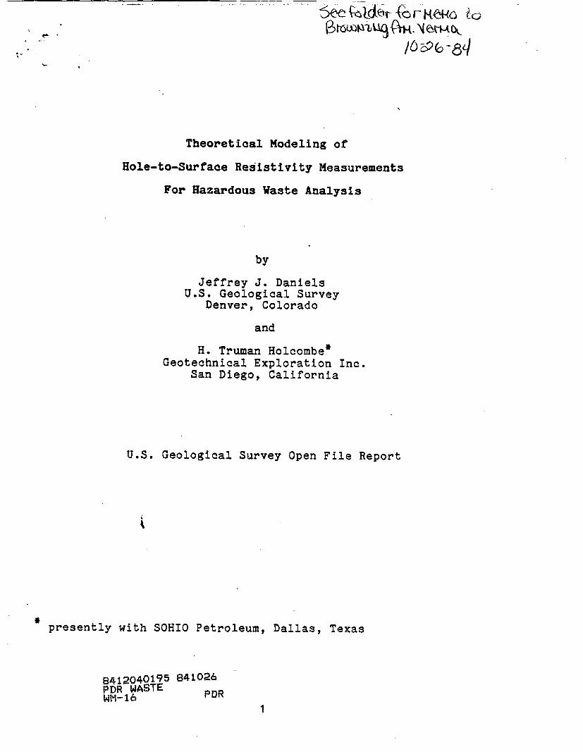
Theoretical Modeling of

Hole-to-Surface Resistivity Measurements

For Hazardous Waste Analysis

by

Jeffrey J. DanielsU.S. Geological Survey

Denver, Colorado

and

H. Truman Holcombe*Geotechnical Exploration Inc.

San Diego, California

U.S. Geological Survey Open File Report

presently with SOHIO Petroleum, Dallas, Texas

B412040195 841026PDR WASTE PDRWM-16

*

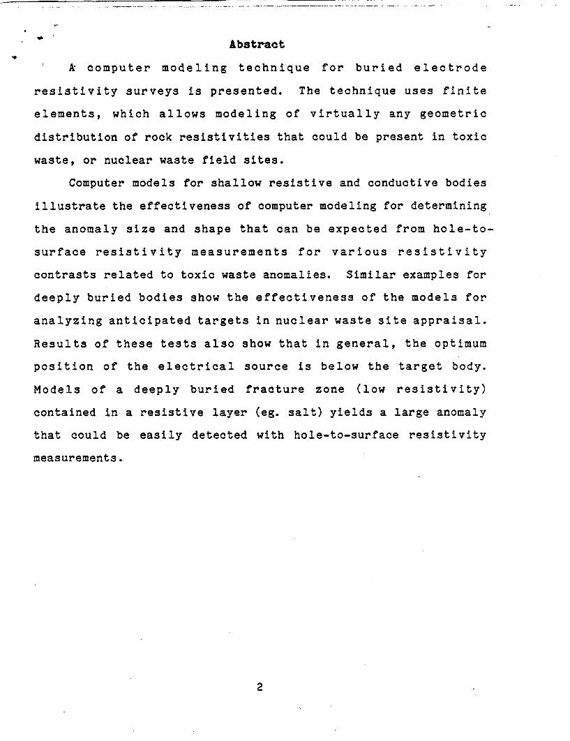
Abstract

A computer modeling technique for buried electrode

resistivity surveys is presented. The technique uses finite

elements, which allows modeling of virtually any geometric

distribution of rock resistivities that could be present in toxic

waste, or nuclear waste field sites.

Computer models for shallow resistive and conductive bodies

illustrate the effectiveness of computer modeling for determining

the anomaly size and shape that can be expected from hole-to-

surface resistivity measurements for various resistivity

contrasts related to toxic waste anomalies. Similar examples for

deeply buried bodies show the effectiveness of the models for

analyzing anticipated targets in nuclear waste site appraisal.

Results of these tests also show that in general, the optimum

position of the electrical source is below the target body.

Models of a deeply buried fracture zone (low resistivity)

contained in a resistive layer (eg. salt) yields a large anomaly

that could be easily detected with hole-to-surface resistivity

measurements.

2

Introduction

The detection of geologic inhomogenities near a hazardous

waste storage area will require the use of techniques that do not

jeopardize the structural integrity of the rock formation with

concentrated drilling. Although surface geophysical techniques

can be used to detect near-surface rock properties, hole-to-

surface resistivity measurements improve the depth penetration

and resolution of resistivity, while minimizing the number of

drill holes needed to evaulate a potential waste repository site.

Hole-to-surface resistivity measurements have been successfully

tested in shallow volcanic rocks ( Daniels, 1978), and

metamorphic rocks (Daniels, 1984)) and in a deeply buried

evaporite sequence (Daniels, 1982).

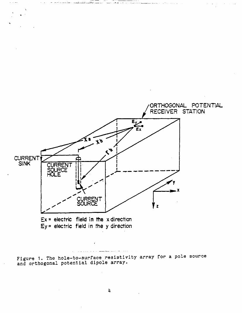
The hole-to-surface resistivity array is illustrated in

Figure 1. Hole-to-surface measurements are made by placing a

pole, or bipole, source down a borehole and measuring the

resulting distribution of the electric potential on the surface.

Previous field studies have shown that the optimum source-

receiver configuration for many applications consists of a pole

source in the borehole, and orthogonal potential dipole

measurements on the surface. A dipole potential receiver,

consisting of closely spaced poles, enables the interpreter to

calculate the approximate total electric field. Non-radial

components of the electric field are zero in a homogenous or

laterally isotropic earth. If lateral inhomogeneities are

present in the geoelectric section, then the direction of the

electric current emanating from a buried current source is not

3

ORTHOGONAL POTENTIALRECEIVER STATION

-OURRENT ISINK CURRENT 1.

SORECE I, J-_ __

,' CUJRRENT, '1 SOURCE / z

Ex = electric field in the x directionEy = electric field in the y direction

Figure 1. The hole-to-surface resistivity array for a pole sourceand orthogonal potential dipole array.

Yadial, and it is necessary to measure two orthogonal components

of the potential in order to measure the total electric field.

Theoretical studies of surface potentials due to in-hole current

sources have been described by Alfano (1962), Merkel (1971),

Merkel and Alexander (1971), Snyder and Merkel (1973), and

Daniels (1977, 1978).

Theoretical solutions for buried electrodes in a one- or

two-layered medium have been given by Daknov (1959), and Van

Norstrand and Cook (1966). Daknov (1959) has shown example curves

for the normal and lateral well logging arrays in the presence of

a resistive layer. Schlumberger departure curves (1972) also use

models of three-layer cases for various well logging arrays.

A theoretical solution to the problem of a buried current

electrode in a three-layered earth with a surface receiver bipole

was first presented by Alfano (1962). Analytic models for a

buried source and surface receiver for a sphere and three-layered

earth models were given by Snyder and Merkel (1973) and Merkel

and Alexander (1971). Daniels (1977, 1978) has presented the

solutions for buried electrodes in an n-layered earth, and for an

arbitrarily shaped three dimensional body in a homogenous

halfspace.

All of the models mentioned above are limited in the

complexities that can be included in the models. The model used

in the study presented in this paper (developed by Holcombe

(1983) under contract to the U.S. Geological Survey)incorporates

several basic model elements (topography, layered earth, multiple

three dimensional bodies) into a single model that can be used to

simulate complex geologic conditions. In addition, the model can

5

be used to simulate any electrode configuration (eg. hole-to-

hole, hole-to-surface, etc.). However, the model results

presented in this paper are restricted to the hole-to-surface

array using a buried pole source, and total field surface

receiver. The models were chosen to illustrate the hole-to-

surface resistivity response for various depths and positions of

the body representing the resistivity contrast with respect to

the current source.

General Description of the Model

The purpose of this algorithm is to provide a capability to

calculate direct current resistivity responses for realistically

complex three-dimensional earth models, that may include

arbitrary topography at the earth-air interface. The algorithm

can be set up to simulate virtually any surface or subsurface

configuration of current and potential electrodes. The algorithm

is currently configured to calculate responses for (1) the

Schlumberger, (2) the dipole-dipole, (3) the hole-to-hole, and

(4) the hole-to-surface electrode configurations.

The computer algorithm makes use of the finite element

method to calculate the electric potential distribution in the

earth about an array of point current sources. The elements have

a convenient hexahedral (rectangular prism) shape to facilitate

the construction of a complex, discrete earth model. The near-

surface layers of elements can be distorted, using an

isoparametric coordinate transformation, to accomodate topography

in the model. This is illustrated in Figure 2, where the dashed

6

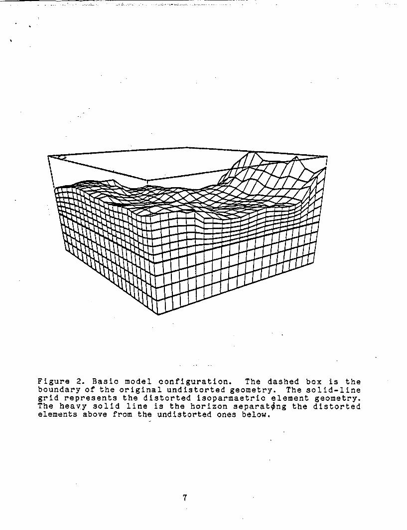
Figure 2. Basic model configuration. The dashed box is theboundary of the original undistorted geometry. The solid-linegrid represents the distorted isoparmaetric element geometry.The heavy solid line is the horizon separating the distortedelements above from the undistorted ones below.

7

b*ox represents the original undistorted geometry and the solid

line grid is the distorted isoparametric element geometry. The

geometric change is accomplished by using a coordinate

transformation which translates the coordinates of the corners of

the elements (which are the locations of the finite element

nodes) vertically downward an appropriate distance. The heavy

solid line is an arbitrarily determined horizon which separates

the distorted elements from the undistorted ones.

The term "isoparametic" refers to the order of the

polynomial form (ie., linear, quadratic, etc.) used to relate the

transformed to the untransformed coordinates. If it is the same

order as the polynomial used to approximate the variation of the

parameter of interest within a finite element, then the distorted

element is called "isoparametric'". The terms "subparametric" and

"superparametric?? are used for transformations of lower or higher

order, respectively.

Theoretical Development

The theoretical resistivity development follows that of

Pridmore and others (1981), with the addition of isoparametric

finite elements near the surface of the earth model to simulate

topography. Isoparametric elements can be distorted to

incorporate an irregular surface without loss of generality.

The domain equation is the steady-state equation of

continuity of current density:

OTC V c=0 (1)

8

where J. is the conduction current density within an arbitrary

volume of the earth when current sources are absent. It is

assumed that the conductivity of the earth is isotropic and a

function of position only. Therefore, Ohm's Law (Jc'= E) can be

substituted into equation (1), and since E= -V7 , then:

-70 V 0r 0 = 0 (2)

whereois the scalar electric potential. When the volume of

earth under investigation contains sources of diverging current,

then

-V -f = V As - (3)

where is is the current density due to the sources.

The finite element method has a long history of success in a

wide variety of applications (Huebner, 1975, p.13- 14) and its

validity for the classic Poisson problem defined by equation (3)

is well established. The domain for the finite element numerical

solution is a model where topography is superimposed upon an

otherwise rectangular prism shaped volume of earth. This model

is divided into hexahedral or distorted hexahedral elements as

shown in Figure 2. The distorted elements are mapped onto a

regular hexahedral array by a vertical coordinate transformation.

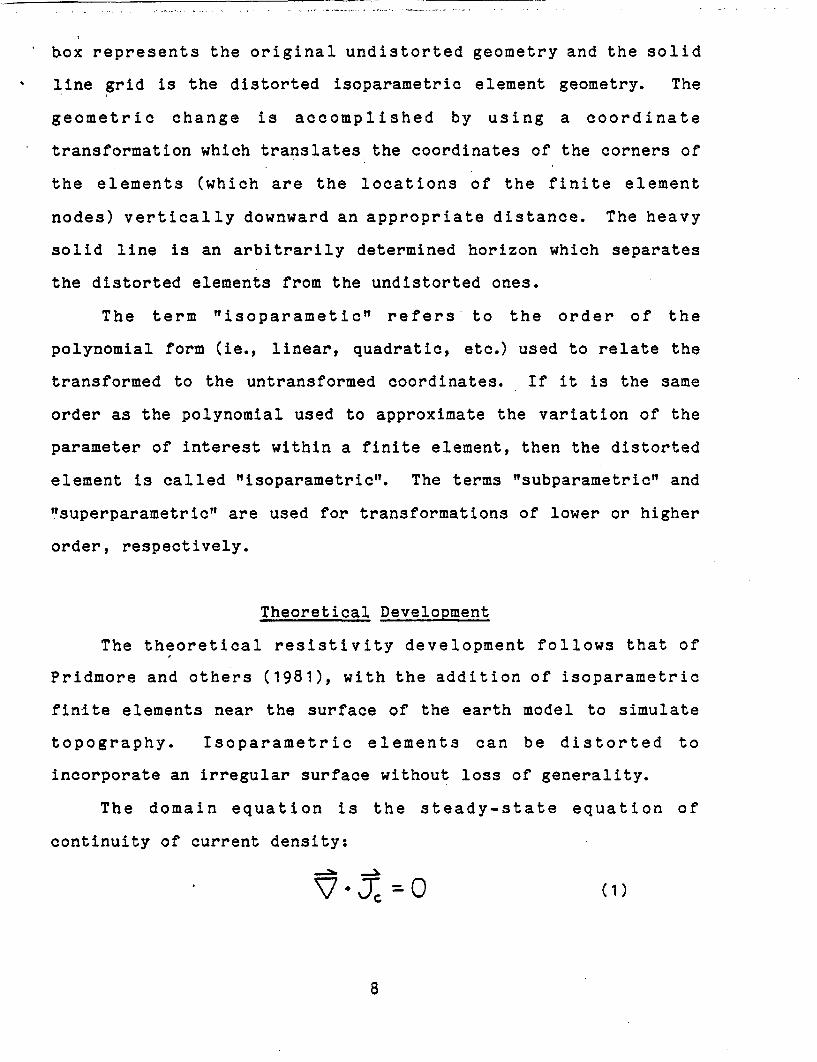
The true solution within each hexahedral finite element (see

Figure 3) is approximated by a trial function of the form:

tI«(U IV$W) z N.,(u,v, w) OL (4)

where the Oils are the nodal values of the electric potential and

the Ni's are the shape functions defined as

N(U,V,w) +i4 U Uj(b vvj)(c'+ vwiP,) (5)

where u,v, and w are Cartesian coordinates in the transformed,

9

.. I...

undistorted finite element space, ui, vi, and wi are the nodal

values and 2a, 2b, and 2c are the u, v, and w dimensions of the

element. This type of element is an isoparametric tri-linear

element of the serendipity class (Huebner, 1975, p. 179-191).

The variational method is chosen for the derivation of the finite

element matrix, although other finite element methods will result

in an identical formulation.

If the equation that the true solution satisfies is known,

then the trial solution given in equation(4) may be forced to

satisfy it. In this case, equation (3) may be written for the

nth finite element in the following operator form:

I-0 < f (6)where L is the Laplacian operatorC-43and f=O, or fzV UsA

depending on whether or not the nth element contains a source.

The minimum theorem (see Mikhlin and Smolitskiy, 1967, p. 147-

155) states that the solution of (6) minimizes the functional,

expressed in inner product form,

F (0) =<LO',> - 2 KO'f) (7)

provided that the following conditions are met:

1. The operator L is self-adjoint and positive definite. Thishas been proven by Pridmore and others (1978).

2. 0 and f are elements of the same Hilbert space. They must bemembers of the subspace of all functions which have continuousfirst derivatives within the nth element.

The inner product notation in equation (7) is defined by

isb) te v (a Cob) a V,,

which is the volume integral over the nth element of the dot

product of functions a, and b. Therefore, for the nth element

iC

I

0(16jbc)

4~,b,--C)

-.-scheme forCoordinate

0 0 nfiguration and nodefinite elementFigure 3*hexahedral

1 1

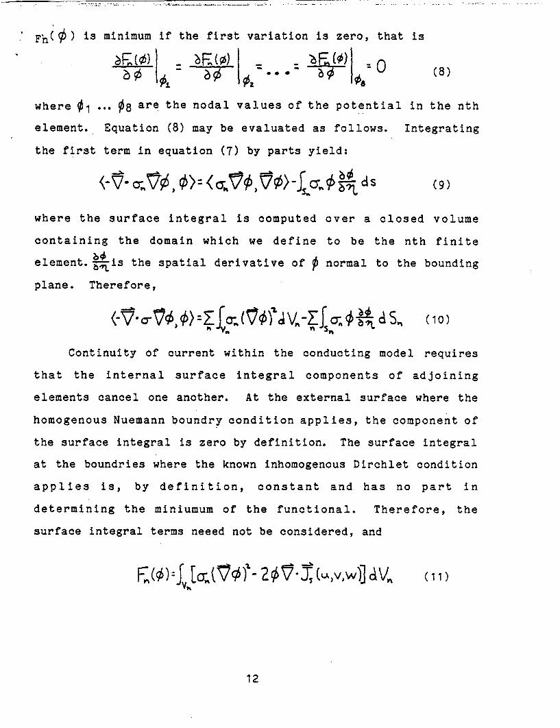
Fnt ) is minimum if the first variation is zero, that is

a___) - _ 0 - ='-'- *F ) I (8)

where 01 ... 08 are the nodal values of the potential in the nth

element. Equation (8) may be evaluated as follows. Integrating

the first term in equation (7) by parts yield:

<-V o;,3X,¢>-<:;0V0>~i5ds (9)

where the surface integral is computed over a closed volume

containing the domain which we define to be the nth finite

element. by-is the spatial derivative of p normal to the bounding

plane. Therefore,

(-Io ar, ) - t (:0 JVE-2j0 ksa +A d Sh ( 1 0)

Continuity of current within the conducting model requires

that the internal surface integral components of adjoining

elements cancel one another. At the external surface where the

homogenous Nuemann boundry condition applies, the component of

the surface integral is zero by definition. The surface integral

at the boundries where the known inhomogenous Dirchlet condition

applies is, by definition, constant and has no part in

determining the miniumum of the functional. Therefore, the

surface integral terms neeed not be considered, and

FnWX-y ~)- f- (" )3 Vn (1

12

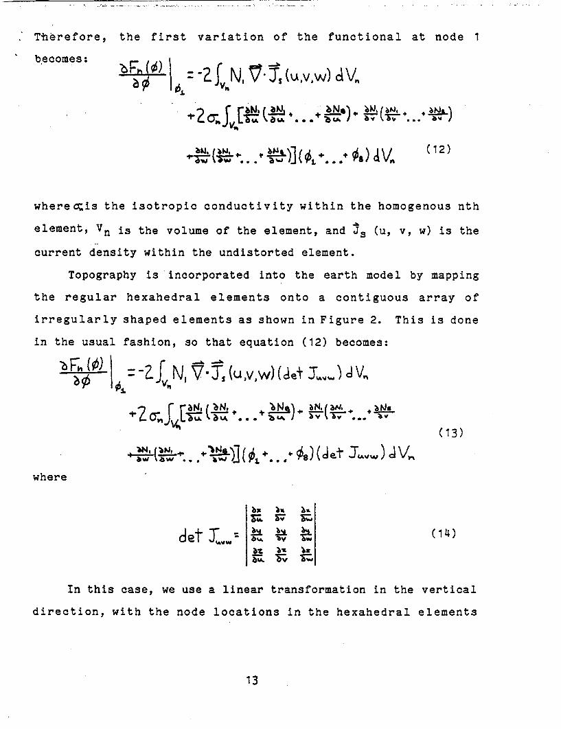
Therefore, the first variation of the functional at node 1

becomes:

2 S to (be by 77^^) abv a

INS ) .. (12)

whereoqis the isotropic conductivity within the homogenous nth

element, Vn is the volume of the element, and J5iu, v, w) is the

current density within the undistorted element.

Topography is incorporated into the earth model by mapping

the regular hexahedral elements onto a contiguous array of

irregularly shaped elements as shown in Figure 2. This is done

in the usual fashion, so that equation (12) becomes:

h(b) 1 L=-Z'JN V J(UVW) Wet T.,) )JV

+2 r ray,(-W I N S) .0 IN. (a. IN aNgAnJL-Ya i%A a .+ .4^ I v ..

where

SePRt T...-h Vu (14)1%~~~~~~~~14

In this case, we use a linear transformation in the vertical

direction, with the node locations in the hexahedral elements

13

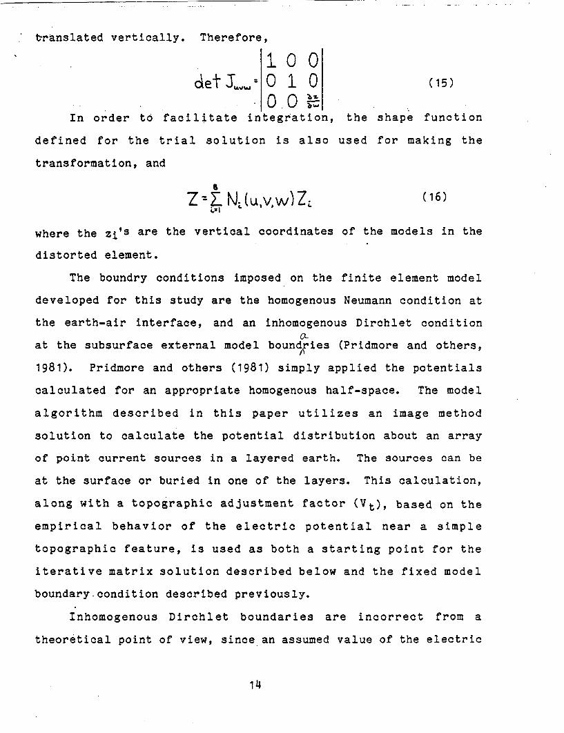
translated vertically. Therefore,

10 0detr L 1 0 (15)

0. 0 i2In order to facilitate integration, the shape function

defined for the trial solution is also used for making the

transformation, and

Z=7 N!(u,V,W)ZL (16)

where the Zi's are the vertical coordinates of the models in the

distorted element.

The boundry conditions imposed on the finite element model

developed for this study are the homogenous Neumann condition at

the earth-air interface, and an inhomogenous Dirchlet conditiono-

at the subsurface external model boundries (Pridmore and others,

1981). Pridmore and others (1981) simply applied the potentials

calculated for an appropriate homogenous half-space. The model

algorithm described in this paper utilizes an image method

solution to calculate the potential distribution about an array

of point current sources in a layered earth. The sources can be

at the surface or buried in one of the layers. This calculation,

along with a topographic adjustment factor (Vt), based on the

empirical behavior of the electric potential near a simple

topographic feature, is used as both a starting point for the

iterative matrix solution described below and the fixed model

boundary condition described previously.

Inhomogenous Dirchlet boundaries are incorrect from a

theoretical point of view, since an assumed value of the electric

14

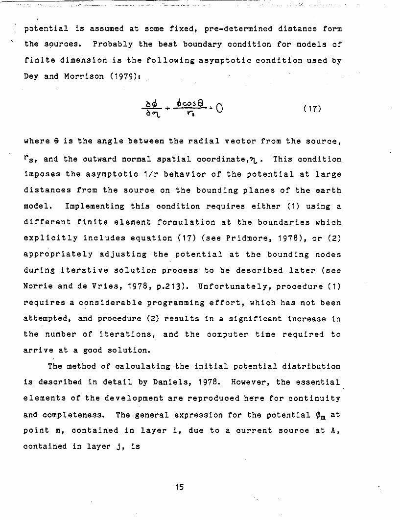
potential is assumed at some fixed, pre-determined distance form

the sources. Probably the best boundary condition for models of

finite dimension is the following asymptotic condition used by

Dey and Morrison (1979):

i + Jocose O t~~~17)

where e is the angle between the radial vector from the source,

rs, and the outward normal spatial coordinated . This condition

imposes the asymptotic 1/r behavior of the potential at large

distances from the source on the bounding planes of the earth

model. Implementing this condition requires either (1) using a

different finite element formulation at the boundaries which

explicitly includes equation (17) (see Pridmore, 1978), or (2)

appropriately adjusting the potential at the bounding nodes

during iterative solution process to be described later (see

Norrie and de Vries, 1978, p.213). Unfortunately, procedure (1)

requires a considerable programming effort, which has not been

attempted, and procedure (2) results in a significant increase in

the number of iterations, and the computer time required to

arrive at a good solution.

The method of calculating the initial potential distribution

is described in detail by Daniels, 1978. However, the essential

elements of the development are reproduced here for continuity

and completeness. The general expression for the potential Om at

point m, contained in layer i, due to a current source at A,

contained in layer J, is

15

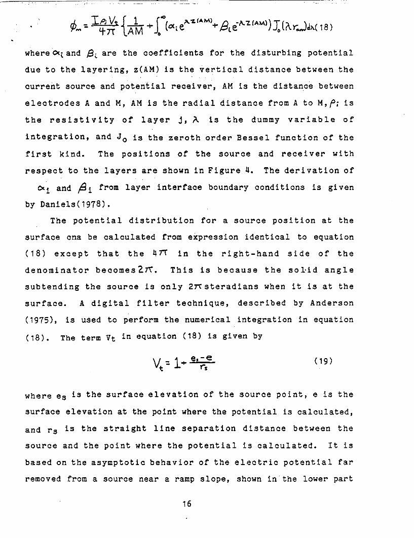
'f XT = {At § j (as +fiebz(^)J(18)

where Oland A are the coefficients for the disturbing potential

due to the layering, z(AM) is the vertical distance between the

current source and potential receiver, AM is the distance between

electrodes A and M, AM is the radial distance from A to M,P; is

the resistivity of layer J, A is the dummy variable of

integration, and JO is the zeroth order Bessel function of the

first kind. The positions of the source and receiver with

respect to the layers are shown in Figure 4. The derivation of

vi and Ai from layer interface boundary conditions is given

by Daniels(1978).

The potential distribution for a source position at the

surface cna be calculated from expression identical to equation

(18) except that the 47T in the right-hand side of the

denominator becomes2N7. This is because the solid angle

subtending the source is only 27-csteradians when it is at the

surface. A digital filter technique, described by Anderson

(1975), is used to perform the numerical integration in equation

(18). The term Vt in equation (18) is given by

V 0 .l+ - (19)

where es is the surface elevation of the source point, e is the

surface elevation at the point where the potential is calculated,

and rs is the straight line separation distance between the

source and the point where the potential is calculated. It is

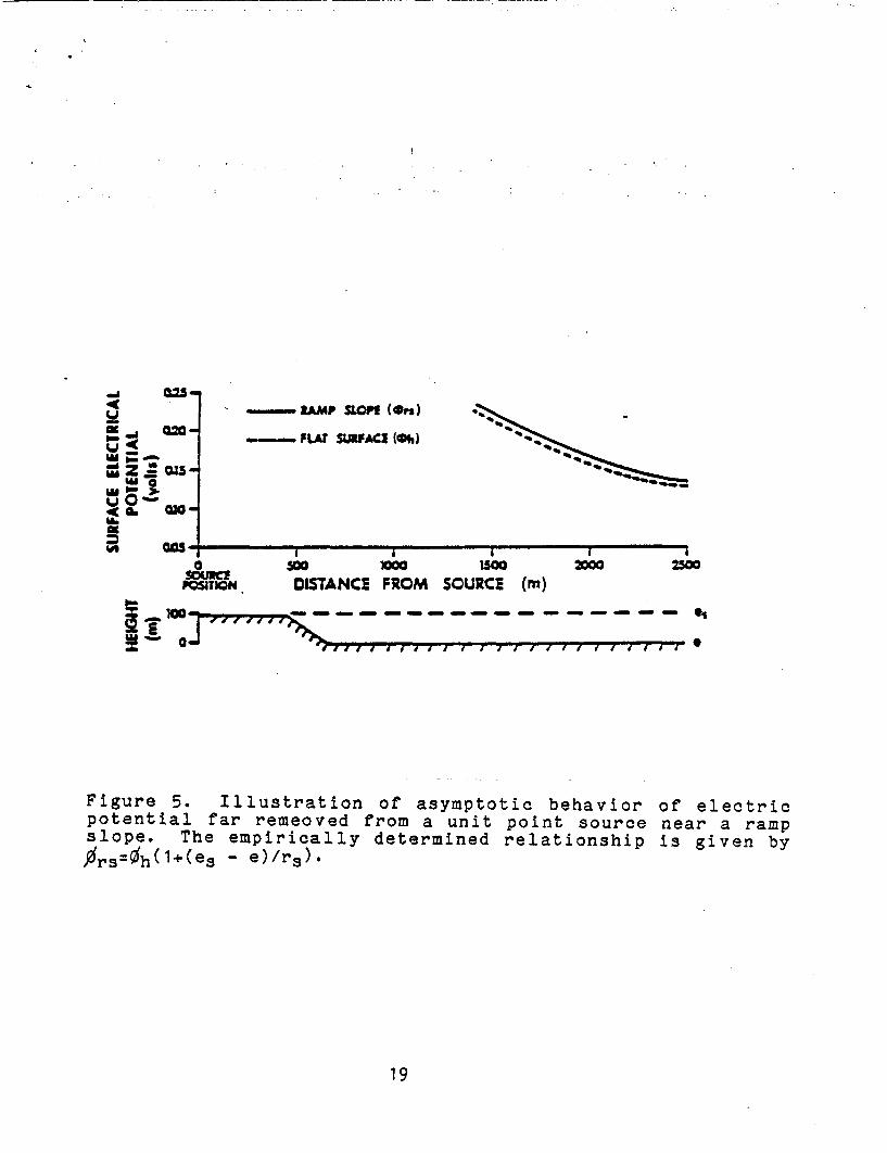
based on the asymptotic behavior of the electric potential far

removed from a source near a ramp slope, shown in the lower part

16

- -+C -I I - -W-A I rear- - N IWIwV[nTIw

: _ _ _ _ _ _ 1 : :

1I 2 '03 h3I; 0

I 14 =Oi.h L~~ i

-A 'Oj'kl

- _

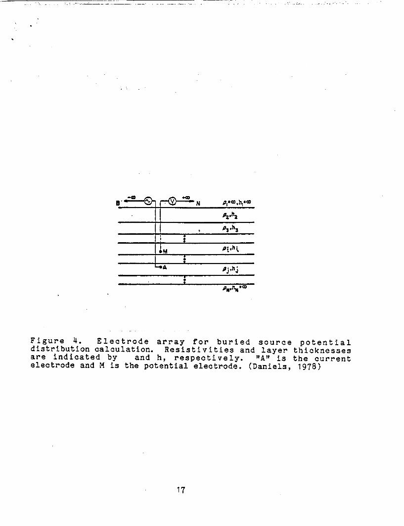
Figure 4. Electrode array for buried source potentialdistribution calculation. Resistivities and layer thicknessesare indicated by and h, respectively. "All is the currentelectrode and M is the potential electrode. (Daniels, 1978)

- 17

of' Figure D. This behavior was determined from a number of

calcualted responses for models containing ramp slope features

like that shown in Figure 5. Incorporating the analytic

multiplier Vt in the original calcualtion. of the potential array,

equation (18) gave a reasonable approximation of the behavior

calculated in the test models at grid locations relatively far

removed from the ramp slope, but should be viewed as a first

order correction. Equation (19) describes the empirical

relationship between the potentials calculated for the ramp slope

(solid line) and a flat surface (dotted line) at distances far

removed for the slope (see Figure 5). This relationship holds

(for relatively small elevation changes ) whether or not the

slope is up or down with respect to the source.

18

-B

do#'Li(S

025

A"MP nLo"E (Mr~s)

in-m FLAT SUACS (h)

1%

I A I

SWo S000 M50

DISTANCE FROM SOURCE (m)

Ioo I

Figure 5. Illustration of asymptotic behavior of electricpotential far remeoved from a unit point source near a rampslope. The empirically determined relationship is given byvrs=h(1+(es - e)/rs).

19

Numerical Solution

The evaluation of the integrals in the functional

(equation 2) are analytic because of the choice of linear

functions for both the trial-solution and the coordinate

transformation. Minimiza ion of the functional (requiring the

first variation to be zero) results in an 8 x 8 matrix equaiton

of the form: Fa, f,

where the L. *: [s8J (20)

where the coefficient matrix Eaij] is symmetric and is usually

referred to as the element matrix. For the simple hexahedral

element (equation 1), there are eight independent coefficients.

In the distorted element (equation ),there are 18 independent

coefficients. Normally, the finite element matrix equations are

assembled into a global matrix and then solved by one of the

matrix inversion techniques commonly used. However, because of

the very large number of elements (sometimes 50,000 or more are

required) the memory requirement for such an inversion far

exceeds the core memory available on even the largest computer.

Therefore, a successive node iterative solution technique was

used, whcih solves only the matrix equations for elements

adjacent %,9 a given node at any particular time. This allows a

reduction in the memory required, but greatly increases the

running time. The solution method chosen is usually called the

successive point over-relaxation (SPOR) method. It is described

in detail in many texts (eg. Ames, 1977, p.119-125). A brief

20

description of the method follows.

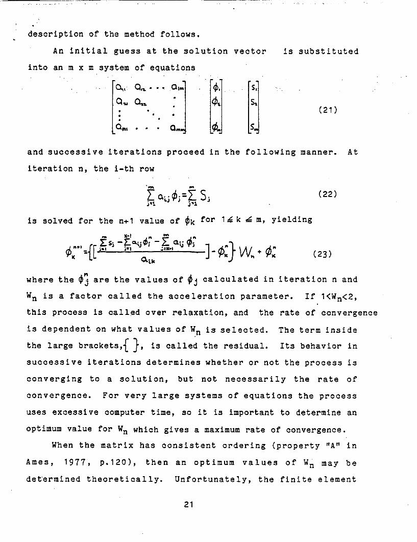
An initial guess at the solution vector is substituted

into an m x m system of equations

., .-- . .'L,.:* II , -6- 5. (21)

Qg^I . * *J

and successive iterations proceed in the following manner. At

iteration n, the i-th row

E: alj Oj Si (22)

is solved for the n-1 value of Ok for 1£z k 4 m, yielding

It { a,, ]" } (23)

where the i are the values of f calculated in iteration n and

Wn is a factor called the acceleration parameter. If 1<Wn<2,

this process is called over relaxation, and the rate of convergence

is dependent on what values of Wn is selected. The term inside

the large brackets,{ }, is called the residual. Its behavior in

successive iterations determines whether or not the process is

converging to a solution, but not necessarily the rate of

convergence. For very large systems of equations the process

uses excessive computer time, so it is important to determine an

optimum value for Wn which gives a maximum rate of convergence.

When the matrix has consistent ordering (property "A" in

Ames, 1977, p.120), then an optimum values of W' may be

determined theoretically. Unfortunately, the finite element

21

formulation used here does not have this property. However,

Carre (1961) and Pridmore (1978) have suggested that Wn should be

the maximum value for which the successive residuals calculated

do not exhibit an oscillatory behavior.

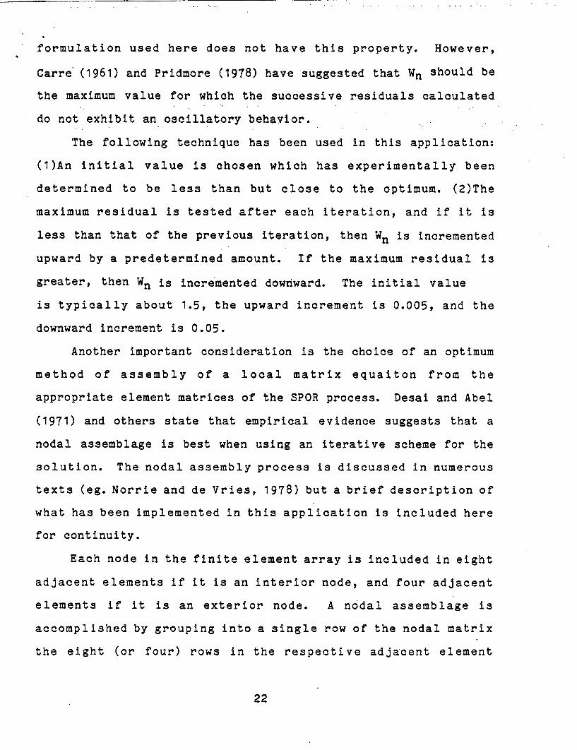
The following technique has been used in this application:

(1)An initial value is chosen which has experimentally been

determined to be less than but close to the optimum. (2)The

maximum residual is tested after each iteration, and if it is

less than that of the previous iteration, then Wn is incremented

upward by a predetermined amount. If the maximum residual is

greater, then Wn is incremented downward. The initial value

is typically about 1.5, the upward increment is 0.005, and the

downward increment is 0.05.

Another important consideration is the choice of an optimum

method of assembly of a local matrix equaiton from the

appropriate element matrices of the SPOR process. Desai and Abel

(1971) and others state that empirical evidence suggests that a

nodal assemblage is best when using an iterative scheme for the

solution. The nodal assembly process is discussed in numerous

texts (eg. Norrie and de Vries, 1978) but a brief description of

what has been implemented in this application is included here

for continuity.

Each node in the finite element array is included in eight

adjacent elements if it is an interior node, and four adjacent

elements if it is an exterior node. A nodal assemblage is

accomplished by grouping into a single row of the nodal matrix

the eight (or four) rows in the respective adjacent element

22

matrices in which the coefficient for the node is contained in

the diagonal position. In the final analysis, each row of the

nodal matrix yields an interpolation of the nodal potential from

-each of' the surrounding 26 nodal values during each iteration,

which is equivalent to a 27 point finite difference

approximation.

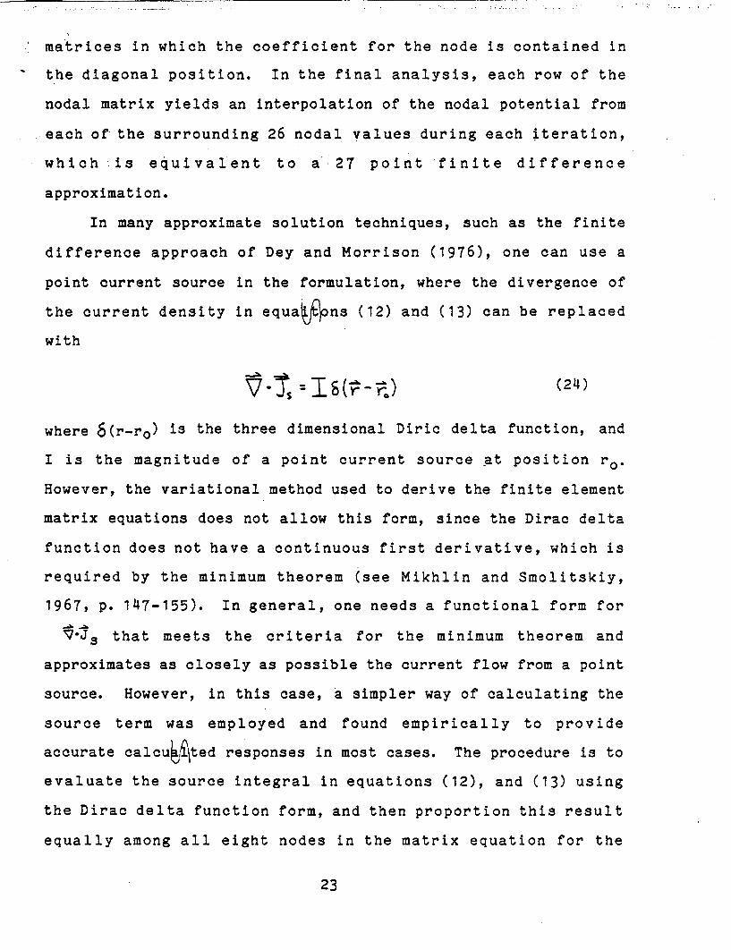
In many approximate solution techniques, such as the finite

difference approach of Dey and Morrison (1976), one can use a

point current source in the formulation, where the divergence of

the current density in equa rons (12) and (13) can be replaced

with

V*:S - I8(r- rO)~~(24)

where 6(r-ro) is the three dimensional Diric delta function, and

I is the magnitude of a point current source at position ro.

However, the variational method used to derive the finite element

matrix equations does not allow this form, since the Dirac delta

function does not have a continuous first derivative, which is

required by the minimum theorem (see Mikhlin and Smolitskiy,

1967, p. 147-155). In general, one needs a functional form for

7 Js that meets the criteria for the minimum theorem and

approximates as closely as possible the current flow from a point

source. However, in this case, a simpler way of calculating the

source term was employed and found empirically to provide

accurate calcu*Ated responses in most cases. The procedure is to

evaluate the source integral in equations (12), and (13) using

the Dirac delta function form, and then proportion this result

equally among all eight nodes in the matrix equation for the

23

finite element containing the source.

The boundary conditions are easily incorporated into the

computer model. The homogenous Neumann condition is a natural

boundary condition of the Poisson equation. It is satisfied

automatically in the finite element formulation when the mesh is

teminated (Norrie and de Vries, 1978, p. 188). The inhomogenous

Dirchlet condition is not a natural boundary condition, but the

finite element formulation derived is still valid when the

condition is imposed (Mikjlin and Smolitskiy, 1967, p. 163). It

is satisfied by simply not performing the nodal calculation at

the appropriate bounding nodes, so that the original calculated

potential values remain the same throughout the iteration

process.

Another important consideration is the determination of

when the solution has converged adequately to be considered

valid. Of equal concern is the practical problem of trying to

minimize the number of iterations required to solve the very

large matrix equation required for this problem. A

straightforward "point-of-diminishing-returns"' argument is used

to determine the optimum point to terminate the iteration

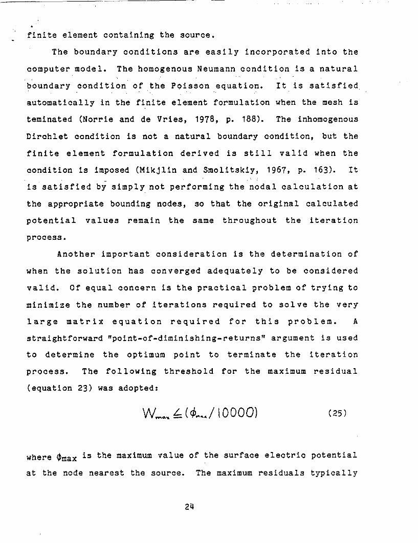
process. The following threshold for the maximum residual

(equation 23) was adopted:

W .ao Ik/1Q0 0) (25)

where Omax is the maximum value of the surface electric potential

at the node nearest the source. The maximum residuals typically

24

ale calculated at or near the sources, and the rest of the

residuals are generally proportional to the nodal electric

potentials. Therefore, if this condition is met, it would

require a large number of additional iterations (perhaps 100, or

more) to make a significant change in the calculated surface

potentials.

Since an isoparametric element matrix contains 18

independent coefficients compared to eight for the regular

hexahedral one, the storage requirements for the global

coefficient array is reduced if as many undistorted

elements as possible are used. Therefore, both types of elements are

included in the computer program. A horizon is determined below

which all the elements are undistorted (Figure 2), and included

in the input to the program. The minimum number of layers of

isoparametric elements needed to adequately approximate the

terrain is included in the model. This has been empirically

determined to be enough layers so that no element has its

vertical dimension reduced to less than one-half of its original

undistorted value.

In order to further minimize the memory required for the

matrix solution, the matrix coefficients are recalculated as

needed in the iteration process. A coefficient array is

calculated and stored for only one finite element layer at a

time. Testing with small arrays indicate that the method costs

only about twice as much as storing the entire array, and yet

reduces the memory required to store the coefficients by an order

of magnitude or more.

If the nodal calculations are performed in the same order

25

in each iteration, the result is an initial asymmetry in the

over-relaxation potentials whfih slows the iteration process.

Therefore, an alternating direction iterative process was

adopted. First, nodal iteration proceeds row by row in each

layer starting from an upper corner and finishing on the

diagonally opposite lower corner. The next iteration begins

where the first stopped and proceeds row by row and layer by

layer in precisely the opposite direction. The iterations are

alternated in this manner through completion of the solution.

This method has been successfully employed by other authors in

similar problems (eg., Gunn, 1964).

A complete listing and operating instructions for the

computer program have bean outlined in detail by Holcombe (1983).

The report by Holcombe (1983) also contains verification tests of

the modeling program, with comparisons to simple models that have

been previously published in the literature.

26

- -

Computer Model Examples

Computer model responses were generated to illustrate what

can be expected from a hole-to-surface resistivity survey for

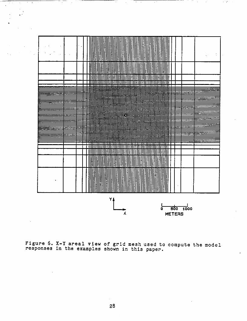
various parameters. The x-y grid used for the finite elements in

the models is shown in Figure 6. The finite elements close to

the source are small (50 m), while the finite element size is

increased away from the source. Computational accuracy is good

for the smaller elements close to the source, and decreases away

from the source. The effects of decreased accuracy away from the

source can be identified by a deteriation of the symmetry of theA

model response at the outer boundry of the finite element grid.

The effects of varying the following parameters are

considered: (1)body size, (2)distance of the source from the

body, (3)vertical position of the source with respect to the

body, and (4)body shape. These situations are illustrated for

resistive and conductive bodies, with deep (500 m, and 700 m) and

shallow (100 m) source positions. The electrode configuration

consists of a pole source, with a total elctric field receiver on

the surface. The response with the body present is normalized to

the response with the body absent (homogenous halfspace, or

layered earth). A normalized response of 1.05 (resistive body) or

0.95 (conductive body) would yield a 5 percent anomaly in the

field, which may be detectable. Responses of 1.01, or 0.99, would

be below the noise level of normal field measurements and would

probably not be detectable.

The effect of varying the body size for a shallow

27

= . . . [ ....H 111111111111111111111111111 I.

_ , ; ; ; ; ; ; ; ; ; ; ; ; ;. .. . . . . .. . . . . . .

= _ _ ; ; ; ; i ; ; ; i ; ; ;........................

_ _ ; ; ; ; ; ; ; ; ~.. . . . .. ... . . .. . . . .

_-_ _ ;; ; ; ; ; ;; : ; ; ; ;. .... ...... ...... . . . .

_ _ _ ; ; ; ; ; ; ; ; ; ; ; ; ; ; , ..... .... ~~~~~. .. .... .. .. .. ...... .. .. .. .. .... .... .. .... .. .. .. ...... .... .. ..... ... I

_ _ ; ; ; ; ; ; ; ; ; ; ;. ...; . .... . .. . . . . . . . .= _ : l: : :: . :. .. :liiliillill------------ I I IT

: L Iililm lilillilillil..........7

1L ~~~~~~~~~~~~~~~.... ...... :t

x o 500 0oo0METERS

Figure 6. X-Y areal view of grid mesh used to compute the modelresponses in the examples shown in this paper.

28

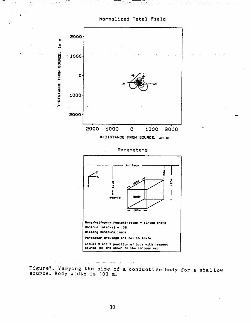
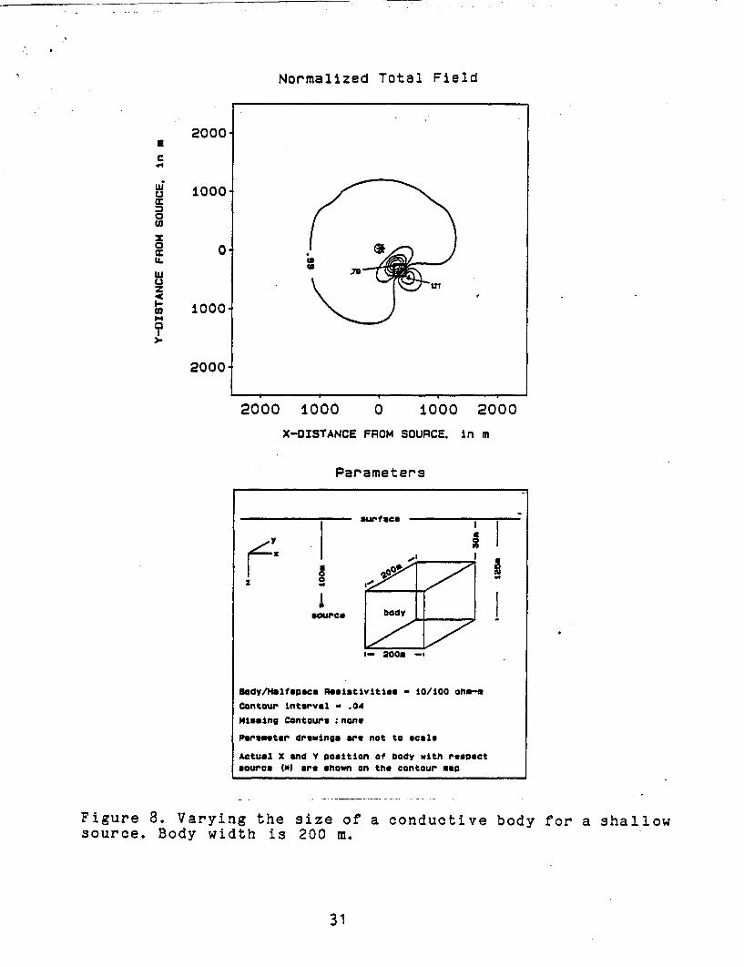
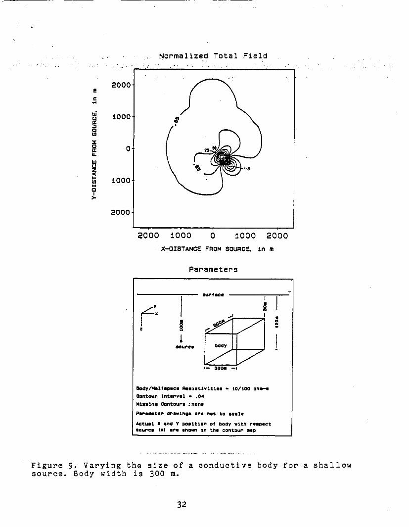
conductive body is shown by comparing Figures 7, 8, and 9. The

top of the body and the source depth in these figures are

constant. Maximum amplitudes of the anomalies are well within

detectability limits, and the size of the anomalies are

a function of the size of the bodies. An anomaly associated with

a conductive body consists of a resistivity low directly over the

body, and an associated resistivity high. The associated

resistivity high is often called a "shadow" anomaly. The size

and amplitude of the shadow anomaly varies with the proximity of

the source to the body, and the intrinsic body parameters (size,

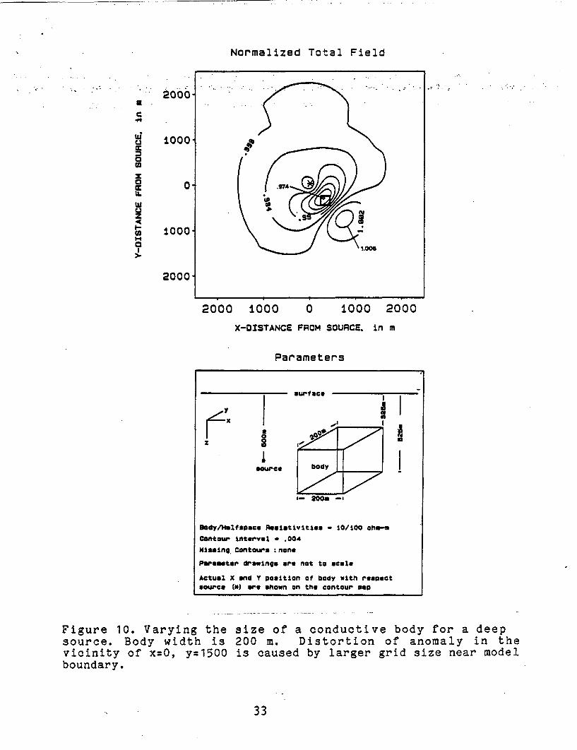
depth, and resistivity). A similar correlation between the size

of the body and the size of the anomaly can be seen for the

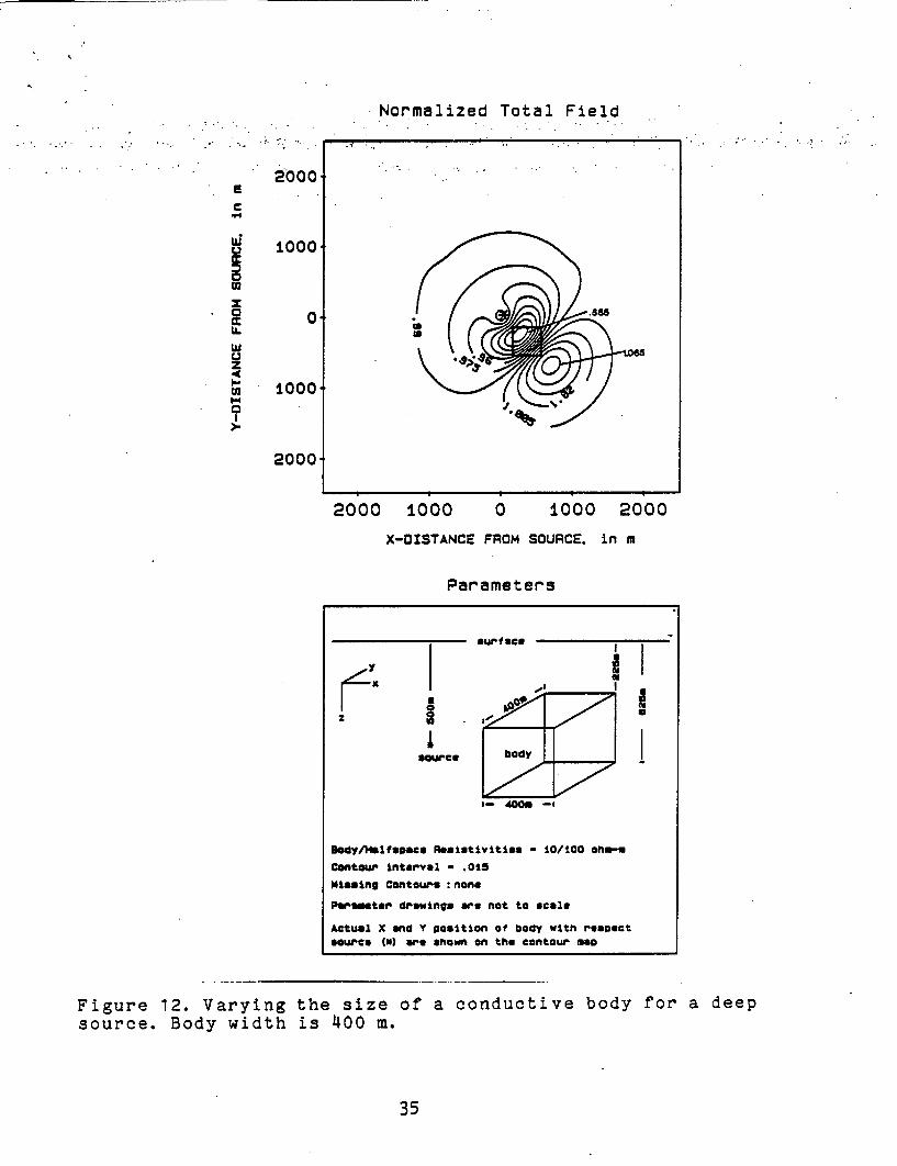
models generated using a deep source (Figures 10, 11, and 12).

These figures for the deep source also illustrate that the areal

size and amplitude of the shadow anomaly is higher for shallower,

and larger bodies.

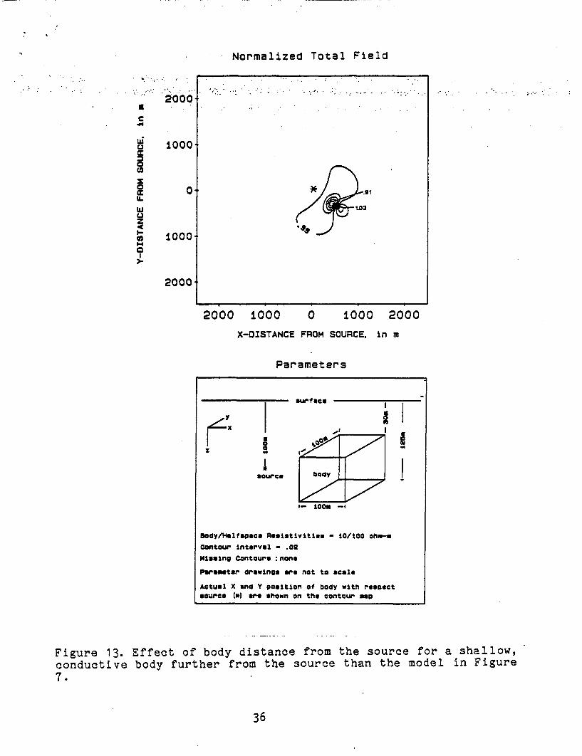
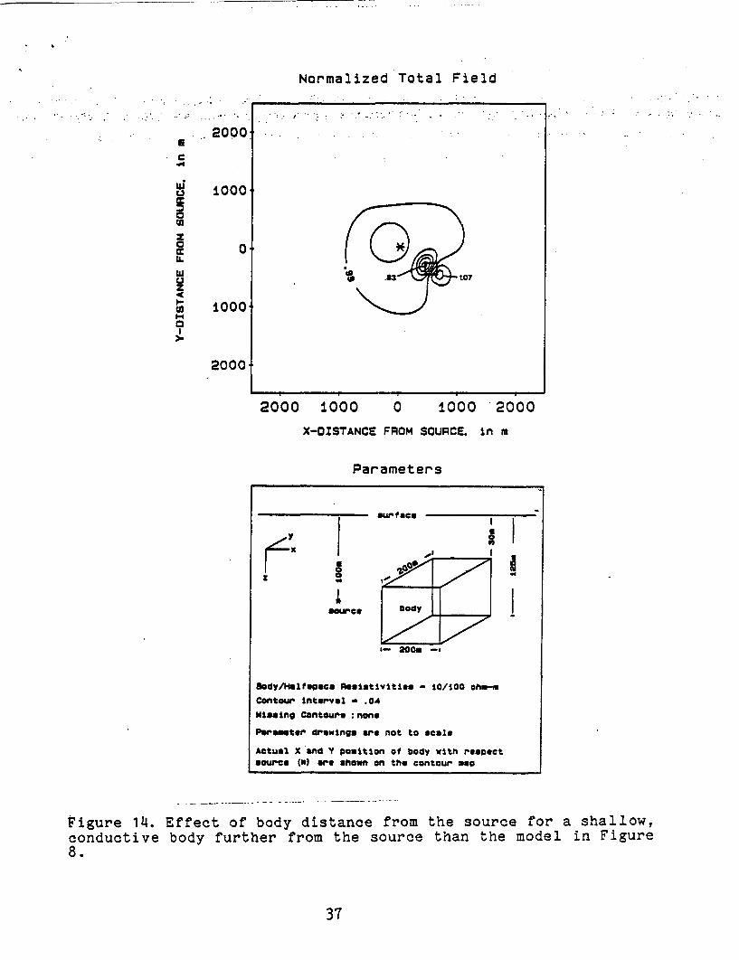
The effect of the distance of the source from the body can

be seen by comparing Figures 13, and, 14 with Figures 7, and 8

respectively. There is very little degradation of the anomaly

amplitudes for the shallow bodies in Figures 13 and 14, in

contrast to the bodies in Figures 7 and- 8 that are closer to the

source. The size of the anomalies are decreased when the source

is further away from the body.

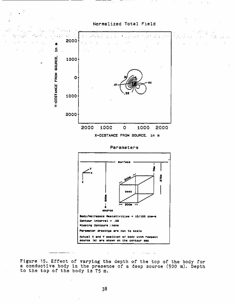
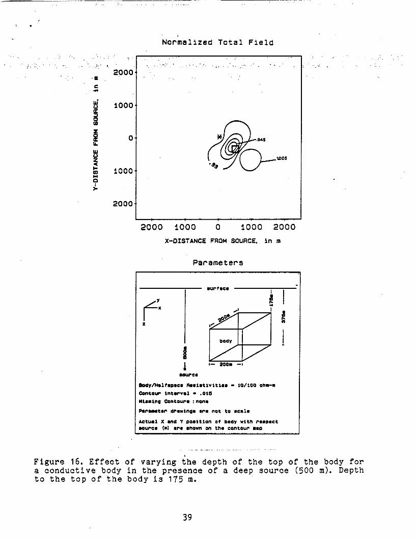
The amplitude and size of the anomaly is strongly dependent

upon the depth to the top of the body. This is illustrated in

Figures 15, 16, and 17 for the deep source. In general, a deep

body results in a broader, lower amplitude anomaly than a shallow

body of the same dimensions. The shadow anomaly also becomes

29

Normalized Total Field

a

uiU

scM

0Wz0E

U.z

0

2000 1000 0 1000 2000

X-OISTANCE FROM SOURCE. in m

Parameters

2

aou#.eu

surtac Lse

I_~~~~~~~a I

'I

86dy/Nalftaeco RosistIvlties - 10/100 ohm-m

Contour Interval - .02Hiaoing Ccntours :lnen

Par_ tor drawings are not to scale

Actual X and Y position of body with respectaourco ( aro shown on the contour map

Figure7. Varying the size of a conductive body for a shallowsource. Body width is 100 m.

30


2000E

IJ 1000.<C3

Ca i000

2000-

2000 1000 0 1000 2000

X-OISTANCE FROM SOURCE, in m

Parameters

I 4IS

0~~~~~~~20

Body/Halfsoaco Realstivities * i0/100 ones

Contour interval - 04

missing Contour* :none

Parameter drawings are not to scael

Actual X and Y pooition of body with respectsource W* are shown on the contour map

Figure 8. Varying the size of a conductive body for a shallowsource. Body width is 200 m.

31

Normalized Total Field;r . . w .I .. ....

KC

w'U

L0W

,0

U.

Uj

U,

0

2000

1000

01

000o.

2000

2000 1000 0 ±000 2000

X-OZSTANCE FROM SOURCE. in m

Parameters

Surf ace

fx

Contour interval - 04Missing CcontourF :none

Pir tor drawings are not to scale

Actual X and: Y position of btody with respectsource (1 are shown an trtc contour moo

Figure 9. Varying the size of a conductive body for a shallowsource. Body width is 300 m.

32


2000

f U

C

.±000awza 0~~

2 ±000

2000 ±000 0 ±000 2000


Parameters

srfacea

source bod -o

Bkdy/Helfspace Rasiativities - 10/100 ohm--a

Contour Interval - .004

Hissing.Contours :none

Persamter drawings aer not to seals

Actual X and Y position of body with respectsource (*Ii art shlown on thu contour sap

Figure 10. Varying the size of a conductive body for a deepsource. Body width is 200 m. Distortion of anomaly in thevicinity of x=0, y=1500 is caused by larger grid size near modelboundary.

33


.. . -~~ . , . ; ... ..

2000-ac..

1000.

W

IaE 0 .4

2000

2000 i000 0 1000 200 0

X-DISTANCE FROM SOURCE. in m

Parameters

s urface

a~~~~~~~~~~~~a

Ux a

0300

2o000l1p0 0ssistivition - 0o00 2000Contour interval - F0UC

Missing Contoure :nono

Pareotor rarwingx are not to scalo

Actuol X and Y position of body with respect*ourco (*1 sre shown an tho contour maD

Figure 11. Varying the size of a conductive body for a deepsource. Body width is 300 m.

34


20004Cc .

1000

z

2 000 . . ,

200

M~ ~ -X

2000 1000 0 1000 2000

X-oISTANCE FROM SOURCE. in m

Parameters

surface

Y~~~~

source body

I-400. -

Body/1tslfspace Resistivitisa - WM10 ohm-a

Contour Interval a .01S

miafing contours :none

paraimeter drawings are not to scale

Actual X and Y position of body with respeCtsource Cm) are shown an the contour mnoo

Figure 12. Varying the size of' a conductive body for a deepsource. Body width is 400Q m1.

35


..4

Ca

0

0

cc

'I-

z4

01I

2000

.... .

.. . . . .

1000.-

0t

1000

2000

2000 1000 0 1000 2000


Parameters

surface

I_ loom 4

Body/Half pecs Rasistivities - 10/t00 ohm-aContour interval - .02

Missing Contour* none

Perametar drawings are not to scale

Actual X and Y position of body with respectoource Cl are shown on the contour map

Figure 13. Effect of body distance from the source for a shallow,conductive body further from the source than the model in Figure7.

36


.2000

.

Ui03

coa:I,

wUZ4

0'-I

10004

0

1000

2000

2000 1000 0 ±000 2000


Parameters

y IRx,

. 200. -.

Bedy/Hmltasoce Resistivities - 10/100 ohm-0tContour interval - .04

Missing Contours none

Parae ter drawings are not to scale

Actual X and Y position of body with respectsource (U) ere shown on the contour map

Figure 14. Effect of body distance from the source for a shallow,conductive body further from the source than the model in Figure8.

37


2000

tr

HU 1000L g '

I

±000U. .

U ±000 .

2000

2000 1000 0 OOO 2000


Parameters

surouse

body

0~~~20

kdy/Nalfspace Resstivitles -1O/iO or.,m



Parametor drawings are not to scale

Actual X and Y position of body with respectsource (m) are shown on the contour moo

Figure 15. Effect of varying the depth of the top of the body fora conductive body in the presence of a deep source (500 m). Depthto the top of the body is 75 m.

38


IC

Uii

CD0

'ULa

I-

0

2000

1000

0'

1000

2000i

2000 1000 0 ±000 2000


Parameters

surface

Zx I

4-I_-fl Ie

body

I-200. -i

sowure

Dody/Halfapaca Rsalativities - 10/100 oIm-a

Contour interval - .01a

Miasing Contours none

Perns tor drawings are not to scale

Actual X and Y position of body with respectsource C are shown on the contour map


39


2000

CE-

1000.

0

0~~0

U v-

*F 1000--

2000

2000 1000 0 1000 2000


Parameters

srace

* 0T

- 200- -,

B0dy/1ofltfaac Reasistvitie - 10/00 ohm-ucontour inteeval - .002Missing Contours none

Parameter drawingo are not to scale

Actual X and Y position of body with resapectsource (*I aor shown an the contour sap


40

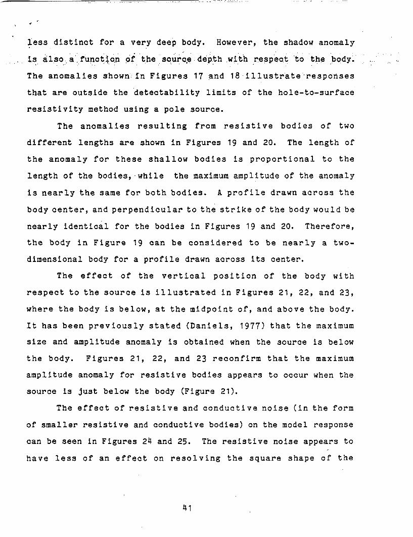
less distinct for a very deep body. However, the shadow anomaly

is also a function of the source depth with respect to the body.

The anomalies shown in Figures 17 and 18 illustrate responses

that are outside the detectability limits of the hole-to-surface

resistivity method using a pole source.

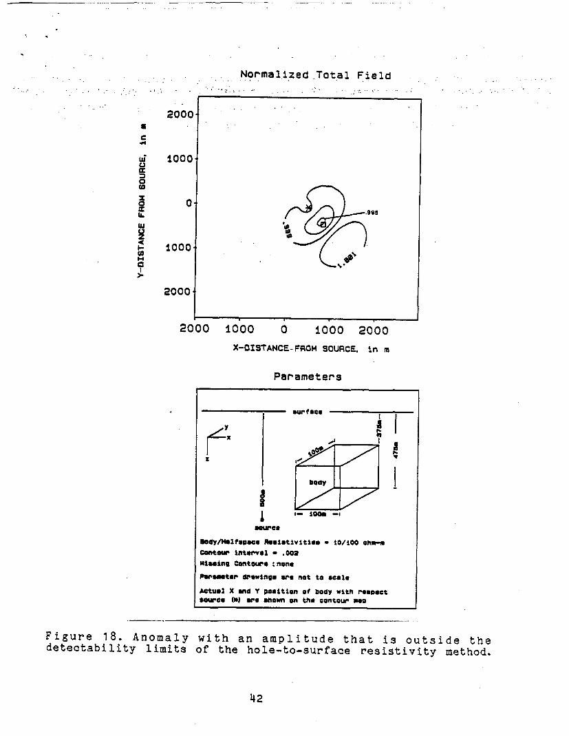
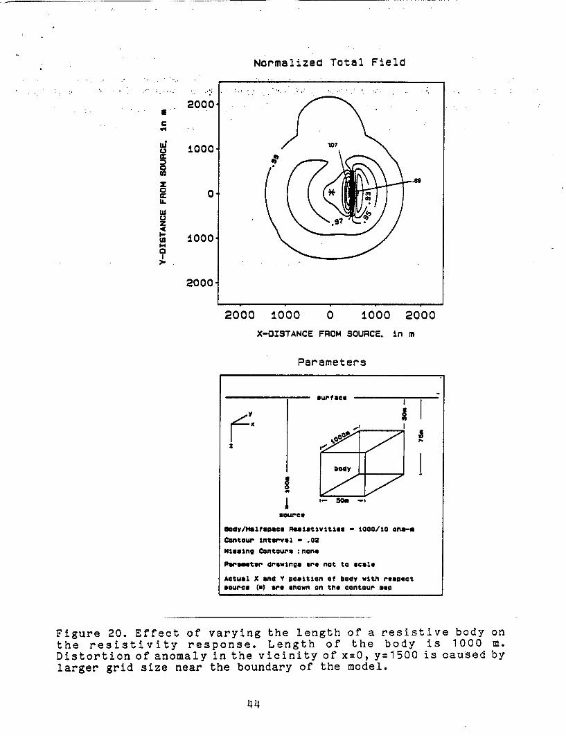
The anomalies resulting from resistive bodies of two

different lengths are shown in Figures 19 and 20. The length of

the anomaly for these shallow bodies is proportional to the

length of the bodies,-while the maximum amplitude of the anomaly

is nearly the same for both bodies. A profile drawn across the

body center, and perpendicular to the strike of the body would be

nearly identical for the bodies in Figures 19 and 20. Therefore,

the body in Figure 19 can be considered to be nearly a two-

dimensional body for a profile drawn across its center.

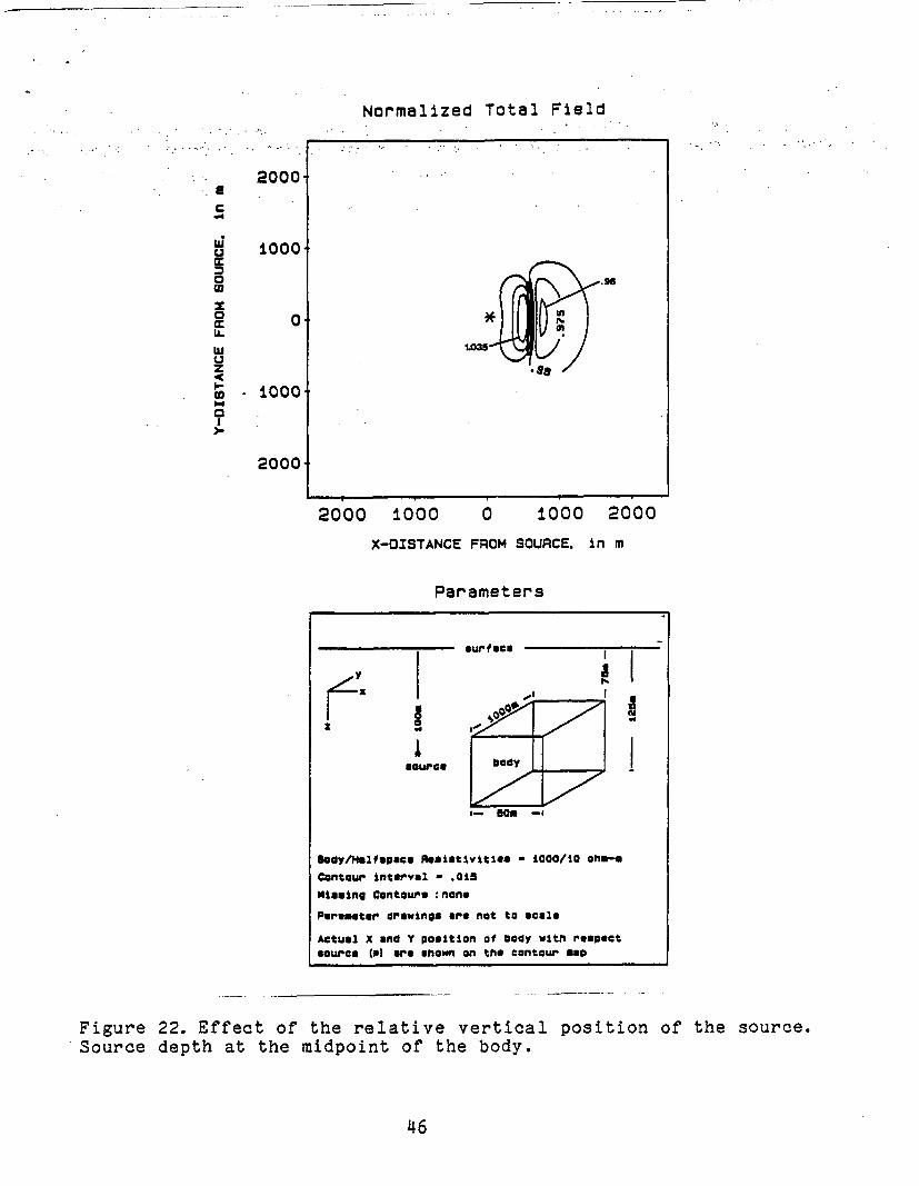
The effect of the vertical position of the body with

respect to the source is illustrated in Figures 21, 22, and 23,

where the body is below, at the midpoint of, and above the body.

It has been previously stated (Daniels, 1977) that the maximum

size and amplitude anomaly is obtained when the source is below

the body. Figures 21, 22, and 23 reconfirm that the maximum

amplitude anomaly for resistive bodies appears to occur when the

source is just below the body (Figure 21).

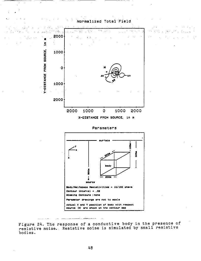
The effect of resistive and conductive noise (in the form

of smaller resistive and conductive bodies) on the model response

can be seen in Figures 24 and 25. The resistive noise appears to

have less of an effect on resolving the square shape of the

Normalized.Total Field.~ ~ ~ . .. ... ... .. . .. .

a

Ca

UzM-Caa

2000

1000

0.

1000.

2000

r | 4 U~~~~~~~~~~~~~~~~~~~~~~~~~~~~~~~~~~~~~~~~~~~~~~~~

2000 1000 0 1000 2000

X-OZSTANCE-FROM SOURCE. in m

Parameters

y

2 ~ ~ ~ ~~~bd

ody/Hsltupeca asieatltvlles - 10/100 M-M

Contoir interval - .002Missing Contour* :none

PWOster drawings are not to scale

Actual X mnd Y position of body witi roeaoctSource (*I are shown an thle contour moo

Figure 18. Anomaly with an amplitude that is outside thedetectability limits of the hole-to-surface resistivity method.

42


2000a

CE.

U

e

Hii

I0

IL

U.

znI-.U,

0

1000

0 0

1000.

2000-

2000 1000 0 ±OO 2000


Parameters

.urf sce

z ~ ~~~~~ I

bodyI

' - *n* -I

source

Body/Haltspac ReAslativites - 1000/10 onh-_

Contour interval - .02

Missing Contours :none

Paraaeter drawings are not to scale

Actual X and Y position of body with respectsource (n) are shown on the contour map

Figure 19. Effect of varying the length of a resistive body onthe resistivity response. Length of the body is 400 m.Distortion of anomaly in the vicinity of x=O, y=1500 is caused bylarger grid size near the boundary of the model.

43


. 2000-

a ,

C

"4.

00

U.z

0

. . .

i000

0'

10OO-

2000-

2000 1000 0 1000 2000


Parameters

f~~~~~~sr | co2 I-

source

bady/Halfsosce 9ea stivities - 1000/10 ohs-a

Contour interval - .02

Missing Contours :none

Parsaeter drawings are not to scale

Actual X and Y position of body with respectsource (*) are shown on the contour map

Figure 20. Effect of varying the length of a resistive body onthe resistivity response. Length of the body is 1000 m.Distortion of anomaly in the vicinity of x=O, y=1500 is caused bylarger grid size near the boundary of the model.


I .

a

U;

0

0

*4

0

2000

1000

0

1000i

2000

2000 1000 0 ±000 2000


Parameters

surface

yfx

body

a~~~a

soureo

Body/Nalfspaee R sistivittls - 1000/10 onm--m

Conteur Interval - .02

Missing Contourx :nono

Peroaeter drawings are not to scale

Actual X and Y position of body with respect

source (*) are shown an the contour map

Figure 21. Effect of the relative vertical position of the source.Source below the body.

45


2000E

1000.0

0 CC ~ 0Is°wU

z i000-

2000-

2000 OOO 0 0O 2000


Parameters

oiureo

i-IOU-_

Body/14lfaspca Resiativitisa - 1000/10 Ohm-0

Contour interval - .015Missing Contour* nono

Paramete drawings are not to scale

Actual X and Y position of body with respectsource (1 are shown an the contour moo

Figure 22. Effect of the relative vertical position of the source.Source depth at the midpoint of the body.

46

Normalized-Total Field-

2000-

1000..976

aw

I

o 01

U ~~~~~~~~~~~~1.024

i 000.

2000

2000 1000 0 1000 2000


Parameters

Isurface-

y I

C ~~source_

I- 50 -I

kdy/HaIf apace Pe 2tivitine - 1000/10 ohm-.

Contour interval - 006missing Contours non,

Parsetsr drawings art not to sCale

Actual X and Y position of body with resooctsource (* are ahown on the contour map

Figure 23. Effect of the relative vertical position of the source.Source above the body.

47


, 2000

U;w

S0

Uz0UaL

0'S

1000

0 , *

.S .W

1000o

2000-

2000 ±0O0 0 1000 2000


Parameters

surface

body

2- 200- -

source

Uody/Ialfapecs Rnsistivitles - 10/100 ohl"



Peraueter drawings ore not to scale

Actual X and Y position of body with respectsource (a) are *sown on the contour map

Figure 24. The response of a conductive body in the presence ofresistive noise.. Resistive noise is simulated by small resistivebodies.

48

*Normalized Total Field

.C. c

Li

0CAz0W

c

w,aU.z4

0

2000'

1000-

04

1000

2000-

2000 OOO 0 1000 2000


Parameters

. body L I

3 -2 0 C m -

aoupce

kdylHelfepace .eiestiviti*e - 10/too oan-.Contour Interval - .02Missing Contours none

Paremeter drawings are not to scale

Actual X and Y position of body with respectsource (J are shown an the contour moo

_ _ _ _ _ _

Figure 25.conductiveconductive

The response of a conductive body in the presence ofnoise. Conductive noise is simulated by small

bodies.

49

conductive body (Figure 24). than the conductive noise (Figure

25).. The amplitude of the main anomalies in both cases are

nearly unaffected by the presence of the interfering bodies.

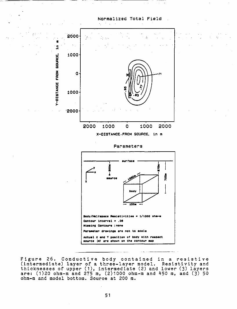
Extremely high amplitude anomalies are seen for the

simulated fracture zone (conductive) contained within a deeply

buried resistive layer (Figures 26, 27, 28, and 29). These

models are directly applicable to hazardous waste sites. The

anomalous response for all of the bodies are 20 to 30 percent

above the response that would be obtained with the fracture zone

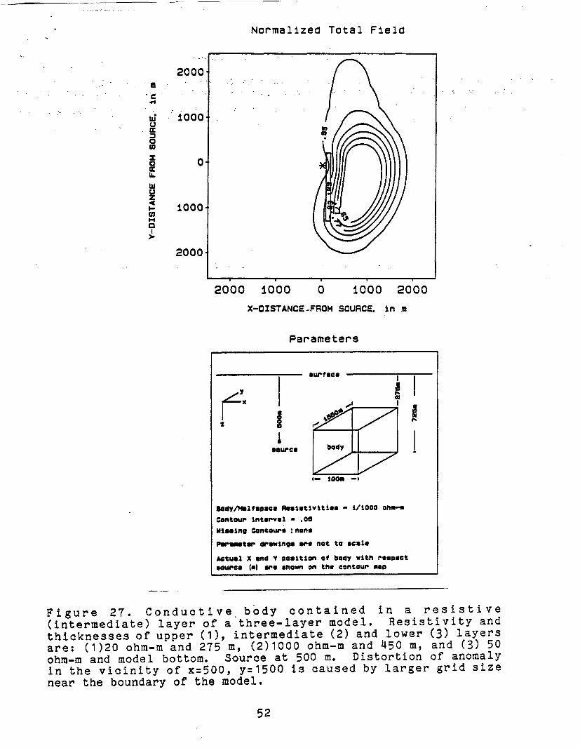
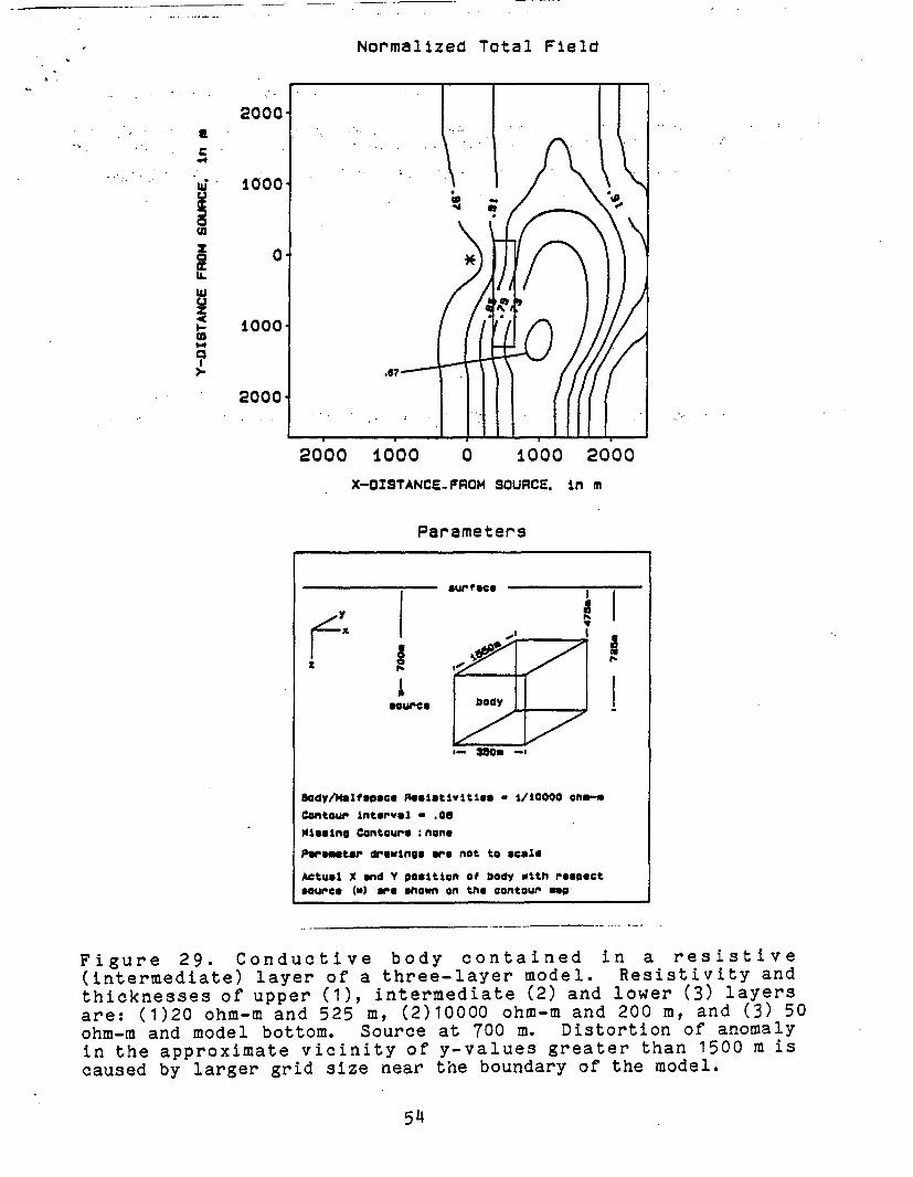
absent from the model. Unfortunately, the model responses in

Figures 27, and 29 also illustrate the limits of the finite

element model for the chosen parameters. The anomalies in both

cases should be nearly symmetrical in both the x-, and y-

directions. The model responses are valid near the center of the

grid, and could be made more accurate near the grid edge by

increasing the number of small grid elements near the grid

boundry.

Conclusions

The finite element computer model developed for simulating

the resistivity response from an arbitrary distribution of

subsurface resistivities provides an excellent means of

predicitng the detectability of anomolous bodies that might be

encountered in hazardous waste site evaluation. Examples for the

hole-to-surface resistivity measurements illustrate that both the

source position and the body depth and dimensions are important

considerations in determining if an anomalous body can be

detected by hole-to-surface resistivity measurements. Therefore,

50


.2000 -

" L 1000.0

oU-

U.~~~~~~~~~~~~~~~~~~~~A

U

g- ±000'U * ~~~~~~~~1 83

0

"2000.

2000 ±000 0 1000 2000

X-DISTANCE-FROM SOURCE. in m

Parameters

surface I

2~

SOO

Body/Haltspsce Reeiutivities - 1/1000 one-.

Contour interval - .0O


Parameter drawings are not to scale

Actuol X snd Y position of body with respect

source () are shown on the contour moo

Figure 26. Conductive body contained in a resistive(intermediate) layer of a three-layer model. Resistivity andthicknesses of upper (1), intermediate (2) and lower (3) layersare: (1)20 ohm-m and 275 m, (2)1000 ohm-m and 450 m, and (3) 50ohm-m and model bottom. Source at 200 m.

51


CaIC

'Uz0

0

2000 1000 0 1000 2000

X-DISTANCE-FROM SOURCE. in m

Parameters

aurTacs

y

a- jO0g -.

Body/Halfaspc RASstivities - i/00 on_Contour Interval - .06Miaaing Contoure none

Parameter drawinog Are not to scale

Actual X and Y position of body with respectsource (*I are ahown on the contour mao

Figure 27. Conductive. body contained in a resistive(intermediate) layer of a three-layer model. Resistivity andthicknesses of upper (1), intermediate (2) and lower (3) layersare: (1)20 ohm-m and 275 m, (2)1000 ohm-m and 450 m, and (3) 50ohm-m and model bottom. Source at 500 m. Distortion of anomalyin the vicinity of x=500, y=1500 is caused by larger grid sizenear the boundary of the model.

52

-


. .~~~~~..2000::*--

Ui .000.

o 0

,- 1000 -

2000

2000 ±000 0 ±000 2000

X-O1STANCE-FROM SOURCE. in m

Par~ameters

surfaeCU'

Contour Interval * .OC4laslng Centoure nene

Peru eter drawings au net te scale

Actuel X and Y position of body with respect*ource VA3 are ahtwn en the eonteur hp0

Figure 28. Conductive body contained in a resistive(intermediate) layer of a three-layer model. Resistivity andthicknesses of upper (1), intermediate (2) and lower (3) layersare: (1)20 ohm-m and 525 m, (2)10000 ohm-m and 200 m, and (3) 50ohm-m and model bottom. Source at 500 m.

53


a.. C

z

0

0

2000 1000 0 1000 2000


Parameters

surface

Ix

50a. -

Body/Maltspece fesativities - 1/10000 aon*


Missing Contours non.

Paraieter drawings are not to scale

Actual X and Y position of body witht respectsource ({) are shown on the contour map

r

Figure 29. Conductive body contained in a resistive(intermediate) layer of a three-layer model. Resistivity andthicknesses of upper (1), intermediate (2) and lower (3) layersare: (1)20 ohm-m and 525 m, (2)10000 ohm-m and 200 m, and (3) 50ohm-m and model bottom. Source at 700 m. Distortion of anomalyin the approximate vicinity of y-values greater than 1500 m iscaused by larger grid size near the boundary of the model.

one of the most important applications of the computer model

presented in this paper will be to design field surveys. The

large anomalies computed for a conductive zone within a deeply

buried resistive layer illustrate the potential usefulness of

hole-to-surface resistivity measurements for hazardous waste

disposal problems.

55

References

Alfano, Luigi, 1962, Geoelectrical prospecting with undergroundelectrodes: Geophys. Prosp., v. 10, p.290-303.

Ames, W.F., 1977, Numerical methods for partial differentialequations: Academic Press, New York.

Anderson, W.L., 1975, Improved digital filters for evaluatingFourier and Hankel transform integrals: NTIS PB-242 800,Springfield, Va.

Carre, B.A., 1961, The determination of the optimum acceleratingfactor for successive over-relaxation: Computer Journal, V. 4, p.73-78.

Dakhnov, V.N., 1959, Geophysical well logging: Quart. Colo.School of Mines, v. 57, 443 p. (translation by G.V. Keller).

Daniels, 1977, Three-dimensional resistivity and induced-polarization modeling using buried electrodes: Geophysics, V. 42,p. 1006-1019.

Daniels, J.J., 1978, Interpretation of buried electroderesistivity data using a layered earth model: Geophysics, v. 43,p. 988-1011.

Daniels, J.J., 1982, Hole-to-surface resistivity measurements atGibson Dome (drill hole GD-1): U.S. Geological Survey Open FileReport 82-320.

Dey, A., and Morrison, H.F., 1976, Resistivity modeling forarbitrarily shaped two-dimensional structures, Parts I and II:Lawerence Berkeley Laboratory Report no. LBL-5223.

Dey, A., and Morrison, H.F.,1979, Resistivity modeling forarbitrarily shaped three-dimensional structures: Geophysics, v.44, p. 753-780.

Gunn, J.E., 1964, The numerical solution of Au.= f by semi-explicit alternating direction iterative method: Numer..Math., v.6, p. 181-196.

Holcombe, H.T., 1982, Terrain effects in resistivity andmagnetotelluric surveys: U.S. Department of Energy Report no.DOE/ID/12038-T1.

Holcombe, H.T. 1983, Three-dimensional isoparametric finiteelement computer algorithm for surface and down-hole DCresistivity applications -- fortran algorithm RES3TA: Report onContract No. 138339-83 for U.S. Geological Survey.

Huebner, K.H., 1975, The finite element method for engineers:John Wiley and Sons, New York.

56

. Merkel, R.H., 1971, Resistivity analysis for plane-layerhAalfspace models with buried current sources: Geophys. Prosp., v.19, p. 626-639.

Merkel, R.H.,' and Alexander, S.S., 1971, Resistivity analysis formodels of a sphere in.a halfspace'with buried current sources:Geophys. Prosp., v. 19, p. 64o-651.

Mikhlin, S.G., and Smolitskiy, K.L., 1967 Approximate methods forsolution of differential and integral equations: Elsevier, NewYork..

Norrie, D.H., and de Vries, G., 1978,An introduction to finiteelement analysis: Academic Press, New York.

Pridmore, D.F., 1978, Three-dimensional modeling of electric andelectromagnetic data using the finite element method: Ph.D.Dissertation, Univ. of Utah, Salt Lake City, Utah.

Pridmore,'D.F.,' Hohmann,' G.W., Ward, S.H., and Sill, W.R., 1981,An investigation of finite element modeling for electrical andelectromagnetic data in three-dimensions: Geophysics, v. 46, p.1009-1024.

Snyder, D.D., and Merkel, R.M., 1973, Analytic models for theinterpretation of electrical surveys using buried currentelectrodes: Geophysics, v. 46, p. 1009-1024.

Van Norstrand, R.G., and Cook, K.L., 1966, Interpretation ofresistivity data: U.S. Geological Survey Professional Paper 499.

57

Documents

U.S. Geological Survey Open File Report 'Theoretical