U.S. Consumer Demand for Alcoholic Beverages: Cross-Section Estimation ofDemographic and Economic Effects

Jirong Wang; X. M. Gao; Eric J. Wailes; Gail L. Cramer

Review of Agricultural Economics, Vol. 18, No. 3. (Sep., 1996), pp. 477-489.

Stable URL:

http://links.jstor.org/sici?sici=1058-7195%28199609%2918%3A3%3C477%3AUCDFAB%3E2.0.CO%3B2-K

Review of Agricultural Economics is currently published by American Agricultural Economics Association.

Your use of the JSTOR archive indicates your acceptance of JSTOR's Terms and Conditions of Use, available athttp://www.jstor.org/about/terms.html. JSTOR's Terms and Conditions of Use provides, in part, that unless you have obtainedprior permission, you may not download an entire issue of a journal or multiple copies of articles, and you may use content inthe JSTOR archive only for your personal, non-commercial use.

Please contact the publisher regarding any further use of this work. Publisher contact information may be obtained athttp://www.jstor.org/journals/aaea.html.

Each copy of any part of a JSTOR transmission must contain the same copyright notice that appears on the screen or printedpage of such transmission.

The JSTOR Archive is a trusted digital repository providing for long-term preservation and access to leading academicjournals and scholarly literature from around the world. The Archive is supported by libraries, scholarly societies, publishers,and foundations. It is an initiative of JSTOR, a not-for-profit organization with a mission to help the scholarly community takeadvantage of advances in technology. For more information regarding JSTOR, please contact support@jstor.org.

http://www.jstor.orgFri Feb 22 14:42:41 2008

U.S. CONSUMER DEMAND FOR ALCOHOLIC BEVERAGES: CROSS-SECTION ESTIMATION OF DEMOGRAPHIC

AND ECONOMIC EFFECTS

Jirong Wartg. X.M. Gao, Eric 3: U'ailes, and Gail L. C r a m e ~

Much research has been done on the control and taxation of alcoholic beverages (Omstein; Atkinson, Gomulka, and Stem; Heien and Pompelli; Johnson et al.; Blaylock and Blisard). The unusual status and attention that alcoholic beverages have attracted is due mainly to their unique characteristics in consumer utilities and social concerns. Consumption of alcoholic beverages has been viewed not only in terms of its effect on individual utility maximization. but also in terms of its bearing on social concerns and government revenue. Although there is empirical evidence suggesting that moderate alcohol consumption lowers the risk of coronary heart disease (e.g. Maclure; Moore and Pearson), social concems are based on the consequences of chronic and acute alcohol abuse. Because of these concerns, they are traditionally subject to some form of social control. One important form of control is the excise tax which contributes significantly to government revenue. The estimation of demand elasticities and the effects of household characteristic variables on alcohol demand provide important information for the formulation of public policies. However, it is with respect to current fiscal deficits and as a means to finance the Clinton administration's proposed program of health care reform that the issue of increased excise taxes on alcoholic beverages has again been discussed as a partial

Jirong Wang is a Research Associate, X.M. Gao is a Research Associate, Eric J. Wailes is a Professor, and Gail L. Cramer is a Professor in the Department of Agricultural Economics and Rural Sociology at the University of Arkansas.

The authors thank Greg Pompelli for helpful suggestions. The helpful comments of two anonymous reviewers. and the RAE editor on an earlier version of this article are gratefully acknowledged.

solution to both fiscal needs and social ills, such as alcoholism and drunk driving fatalities.

Unlike the analysis in Gao et al. using an individual consumption survey, this study analyzes the 1987 to 1988 United States Department of Agriculture (USDA) household food consumption survey data. The survey contains data on quantities and values of over 1,000 food items for at-home consumption, with 1,152 households reporting alcoholic beverage purchase or consumption. Alcohol expenditure cannot be distinguished from away-from-home food expenditure. Data on food used in each household were collected during a seven-day period in personal in-house interviews with the individual recognized as being most responsible for food planning and preparation.' The household characteristic variables include region, household head status, race, season of survey, education, household members by age group, sex, income, urbanization. and household size.

A two-stage budgeting decision model is used in this study. For the first stage, consumers decide whether and how much alcoholic bever- ages to consume. Households that consume any alcoholic beverage (beer, spirits, and wine) during the survey week are studied in compari- son with all surveyed households. The effects of

'The weaknesses of this data set include a relatively low response rate of 38 percent. Demographic characteristics of the participating households were compared with the Current Population Su~vey (Bureau of Labor Statistics and Census), which revealed the sample under-represented a number of demographic groups including: central-city households, higher-income households, and households with a female head. Greater detail on the survey design is found in E~~aluarionof Nonresponse in the Nationwide Food Consumption Survey 1987-88 (United States Department of Agriculture) and Nutrition Monrtoring, Mismanagement of Nutrition Survev Has Resulted in Questio~~able Data -(Government Accounting Office).

Retfew of Agricultural Economics 18(1996):477-489 Copyright 1996 North Central Administrative Committee

478 REVIEW OF AGRICULTURAL ECONOMICS, Vol. 18. No. 3, September 1996

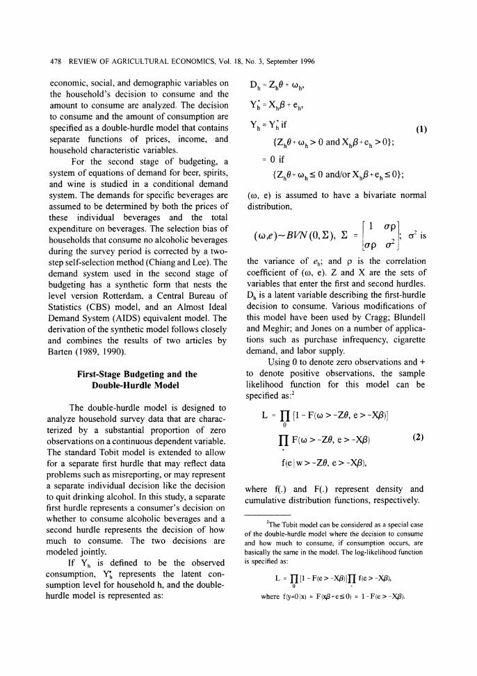
economic, social, and demographic variables on the household's decision to consume and the amount to consume are analyzed. The decision to consume and the amount of consumption are specified as a double-hurdle model that contains separate functions of prices, income, and household characteristic variables.

For the second stage of budgeting, a system of equations of demand for beer, spirits, and wine is studied in a conditional demand system. The demands for specific beverages are assumed to be determined by both the prices of these individual beverages and the total expenditure on beverages. The selection bias of households that consume no alcoholic beverages during the survey period is corrected by a two- step self-selection method (Chiang and Lee). The demand system used in the second stage of budgeting has a synthetic form that nests the level version Rotterdam, a Central Bureau of Statistics (CBS) model, and an Almost Ideal Demand System (AIDS) equivalent model. The derivation of the synthetic model follows closely and combines the results of two articles by Barten (1989, 1990).

First-Stage Budgeting and the Double-Hurdle Model

The double-hurdle model is designed to analyze household survey data that are charac- terized by a substantial proportion of zero observations on a continuous dependent variable. The standard Tobit model is extended to allow for a separate first hurdle that may reflect data problems such as misreporting, or may represent a separate individual decision like the decision to quit drinking alcohol. In this study, a separate first hurdle represents a consumer's decision on whether to consume alcoholic beverages and a second hurdle represents the decision of how much to consume. The two decisions are modeled jointly.

If Y, is defined to be the observed consumption, Y', represents the latent con-sumption level for household h, and the double- hurdle model is represented as:

YA = X,p + e,,

(o , e) is assumed to have a bivariate normal distribution,

the variance of e,; and p is the correlation coefficient of ( o , e). Z and X are the sets of variables that enter the first and second hurdles. D, is a latent variable describing the first-hurdle decision to consume. Various modifications of this model have been used by Cragg; Blundell and Meghir; and Jones on a number of applica- tions such as purchase infrequency, cigarette demand, and labor supply.

Using 0 to denote zero observations and + to denote positive observations, the sample likelihood function for this model can be specified as:2

where f(.) and F(.) represent density and cumulative distribution functions, respectively.

he Tobit model can be considered as a special case of the double-hurdle model where the decision to consume and how much to consume, if consumption occurs, are basically the same in the model. The log-likelihood function is specified as:

L = V I1- F(e> W ) ] n fie > W I .

where f(y=OIx) = F(x@+esO)= t - F ( e > - W ) .

U.S. CONSUMER DEMAND FOR ALCOHOLIC BEVERAGES Wang. Gao. Wailes. Crarner 479

Since the two error terms in the two hurdles have bivariate normal distributions, F(Zh6' + oh > 0, X,p + e, >0) can also be denoted as @(ZO, Xpio, p). The marginal density in the last term of equation (2) can be obtained by integrating over the relevant range of o for the positive observations to give the truncated density of e as:

m

/ f (w)f(e I w)de

f(e / w >-ZB,e> -X@) = " m m

Assuming that the conditional distribution of D, given Y, = Y', is normal with mean Zh6' + po.'(Y, - X$) and that the variance 1 - p-2, equation (3) is simplified as:

where (b is the standard normal distribution density function. Substituting equation (4) into equation (2), the sample likelihood function becomes:

When p = 0, equation (5) gives the likelihood function for the Cragg model. Further, when 9 = Pio, the Tobit model is demonstrated. The GAUSS package is used for optimizing equation (5) which provides a standard bivariate normal cumulative distribution function procedure.

Second-Stage Budgeting and a Synthetic Demand Model

For the second stage of budgeting, estimation of a system of conditional demand for alcoholic beverages can be used to identify the impacts of social and economic variables on demands for beer, spirits, and wine. Price and income (expenditure) elasticities calculated from the conditional system are, therefore, partial elasticities in the sense that the second-stage budgeting has no complementary effects on the first-stage budgeting. A synthetic demand system parallel to that developed by Barten (1990) for a differential model will be used here. The synthetic demand system, which is constructed by artificially nesting the level version Rotter- dam, CBS, and AIDS models, is more general than the individual nested models.

The level version Rotterdam model has the specification (Barten 1989):

where LnQ = w,Lnqj is a Stone quantity J

index. The constant parameters (8,and s,,) in this model are both the marginal budget shares and the Slutsky coefficients. They have the same interpretation as the conventional Rotterdam model. Substituting the relationship 0, = w, + b, into equation (6) ,where b, is assumed constant, the new demand system has the form:

giving the level CBS Model (Keller and Van Driel).

To derive the commonly-used AIDS model, another transformation is made by assuming the following relationship (Deaton and Muellbauer):

480 REVIEW OF AGRICULTURAL ECONOMICS. Vol. 18. No. 3, September 1996

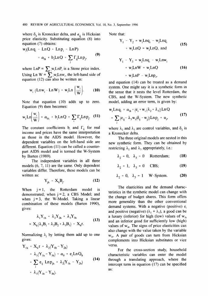
where 6 , is Kronecker delta. and E. . is Hicksian Note that: price elasticity. Substituting equa?ion (8) into equation (7) obtains:

\ ,

wl(Lnqi - LnQ + Lnp , - LnP) + wiLnQ = wiLnQ, and

where LnP = ,w,LnP, is a Stone price index.

Using Ln W = z,w,Lnw,, the left-hand side of equation (12) can also be written as:

Note that equation (10) adds up to zero. Equation (9) then becomes:

The constant coefficients b, and TI, for real income and prices have the same interpretation as those in the AIDS model. However, the dependent variables on the left-hand side are different. Equation (I I) can be called a counter- part AIDS model and is termed the W-System by Barten (1989).

The independent variables in all three models (6, 7, I I) are the same. Only dependent variables differ. Therefore, these models can be written as:

YJh = XhBi. (12)

When j = l , the Rotterdam model is demonstrated; when j = 2 , a CBS Model; and when j = 3, the W-Model. Taking a linear combination of these models (Barten 1990), gives:

Normalizing A, by letting them add up to one gives:

'{h = 'hr A 2 ( Y l h - '2h)+

and equation (14) can be treated as a demand system. One might say it is a synthetic form in the sense that it nests the level Rotterdam, the CBS, and the W-System. The new synthetic model, adding an error term, is given by:

wi Ln q, = aoi+ (e,+ wi ( A 2 + A,)) Ln Q

+ (eij- A3wi(aij- w,))Lnpj + ul, (17)

j

where h?and A, are control variables, and 6,, is a Kronecker delta.

The three original models are nested in this new synthetic form. They can be obtained by restricting h, and h, appropriately, i.e.:

A, = 0, A, = 0 Rotterdam; (18)

A, = 1, A, = 0 CBS; (19)

The elasticities and the demand charac- teristics in the synthetic model can change with the change of budget shares. This form offers more generality than the other conventional demand systems. With a negative (positive) e, and positive (negative) (h?+ A,),a good can be a luxury (inferior) for high (low) values of w,,, and an inferior good for sufficiently low (high) values of w,,. The signs of price elasticities can also change with the value taken by the variable w,,. A pair of goods can turn from Hicksian complements into Hicksian substitutes or vice versa.

For the cross-section study, household characteristic variables can enter the model through a translating approach, where the intercept term in equation (17) can be specified as:

U.S. CONSUMER DEMAND FOR ALCOHOLIC BEVERAGES Wang, Gao, Wailes. Cramer 481

where h, is household characteristic variables. Selection bias in this model is corrected by a two-step process (Heien and Wessells; Chiang and Lee). The decision to consume or not to consume can be indicated by a binary variable, which is a function of latent variables and is estimated as a probit model. The household having zero consumption is censored by an undesirable decision variable that induces the decision not to consume the good during the week-long survey period.

For the iLh good in the hth household, the inverse Mills ratio:

is computed, where P,, is a vector of prices for the hth household, and H, is a vector of house- hold characteristic variables. In this case, $ and 0 are the density and cumulative probability functions, respectively. For those households that do not consume the commodity, the inverse Mills' ratio has denominator (1 - O(Ph, H,)). These inverse Mills' ratios are then used as an instrument in the second stage of estimation. The synthetic model, including household charac- teristic variables and the Mills' ratio, is defined as:

where the adding-up condition, in addition,

requires a,=0 and ykl= 0. The likelihood i I

ratio test can be used to test the restrictions (18 to 20).

One problem with estimating the above demand model is the missing prices for house- holds that did not consume the commodities. These prices are estimated by using prices from

purchasing households regressed on dummy variables such as region, season, and income. The properties of this method are discussed in Gourieroux and Monfort, and Heien and Wessells.

In the survey data, households reported both expenditures and physical quantities. Price data were not collected. Therefore, prices (or "unit values" following Deaton) are obtained by dividing expenditures by physical quantities. The price calculated in this way also reflects consumers' choice of quality of the commodity. Therefore, the calculated price should be adjusted for quality variations before it can be used to estimate commodity demand functions from cross-sectional data.' The quality adjust- ment of prices is performed following Cox and Wohlgenant.

Two-Stage Budgeting and Perfect Price Aggregation

A two-stage budgeting occurs when the consumer can allocate total expenditure in two stages; at the first stage, expenditure is allocated to broader groups of goods, while at the second stage, group expenditures are allocated to the individual commodities. The two-stage budgeting involves both aggregation and separable decision making. To focus attention on three alcoholic beverages (beer, wine, and spirits), this study takes aggregate alcohol consumption as the first- stage decision and the consumption of three beverages as the second-stage d e ~ i s i o n . ~ The two stages are linked by price aggregation, which takes into consideration intragroup substitutions possibly due to detailed price changes among three alcoholic beverages (Ander~on).~

In this article, a generalized Engel demand function is used at the upper level and a syn- thetic demand function, which has a generalized

' ~ a w k a n i has discussed implications when price is measured with error.

4The weak separability between non-alcoholic drinks and alcoholic beverages was tested using a level Rotterdam model. The results failed to reject the hypothesis that alcoholic beverages are weakly separable from other drinks.

'For the limited objectives of this article, the two stages are not estimated iteratively, which would be consistent with the price aggregation theory (Anderson).

482 REVIEW OF AGRICULTURAL ECONOMICS, Vol. 18, No. 3, September 1996

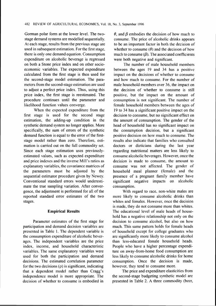
Gorman polar form at the lower level. The two- stage demand systems are modelled sequentially. At each stage, results from the previous stage are used in subsequent estimation. For the first stage, there is only one demand equation. Consumption expenditure on alcoholic beverage is regressed on both a Stone price index and on other socio- economic variables. The expected expenditure calculated from the first stage is then used for the second-stage model estimation. The para- meters from the second-stage estimation are used to adjust a perfect price index. Thus, using this price index, the first stage is reestimated. The procedure continues until the parameter and likelihood hnction values converge.

When the expected expenditure from the first stage is used for the second stage estimation, the adding-up condition in the synthetic demand system no longer applies. More specifically, the sum of errors of the synthetic demand function is equal to the error of the first- stage model rather than zero. Therefore, esti- mation is carried out on the full commodity set. Since each stage estimation uses previously-estimated values, such as expected expenditure and price indexes and the inverse Mill's ratios as explanatory variables, the covariance matrices of the parameters must be adjusted by the sequential estimator procedure given by Newey. Conventional standard errors would underesti- mate the true sampling variation. After conver- gence, the adjustment is performed for all of the reported standard error estimates of the two stages.

Empirical Results

Parameter estimates of the first stage for participation and demand decision variables are presented in Table 1. The dependent variable is the consumption expenditure of alcoholic bever- ages. The independent variables are the price index, income, and household characteristic variables. The same explanatory variables were used for both the participation and demand decisions. The estimated correlation parameter for the two decisions (p) is significant, indicating that a dependent model rather than Cragg's independence model is more appropriate. The decision of whether to consume is embodied in

8, and /3 ernbodies the decision of how much to consume. The price of alcoholic drinks appears to be an important factor in both the decision of whether to consume ( 8 ) and the decision of how much to consume (P ) The associated coefficients were both negative and significant.

The number of male household members between the ages 19 and 34 has a positive impact on the decisions of whether to consume and how much to consume. For the number of male household members over 36, the impact on the decision of whether to consume is still positive, but the impact on the amount of consumption is not significant. The number of female household members between the ages of 19 to 34 has a significant positive impact on the decision to consume, but no significant effect on the amount of consumption. The gender of the head of household has no significant impact on the consumption decision, but a significant positive decision on horn' much to consume. The results also indicate that families who consulted doctors or dieticians during the last year regarding nutritional matters are less likely to consume alcoholic beverages. However, once the decision is made to consume, the amount to consume was not affected. The gender of household meal planner (female) and the presence of a pregnant family member have significant negative impacts on alcoholic consumption.

With regard to race. non-white males are more likely to consume alcoholic drinks than whites and females. However. once the decision is made, they do not consume more than whites. The educational level of male heads of house- hold has a negative relationship not only on the decision to consume alcohol, but also on how much. This same pattern holds for female heads of household except for college graduates who are significantly more likely to consume alcohol than less-educated female household heads. People who have a higher percentage expendi- ture on away-from-home food consumption are less likely to consume alcoholic drinks for home consumption. Once the decision is made, however, they tend to consume more.

The price and expenditure elasticities from the second-stage budgeting synthetic model are presented in Table 2. A three commodity (beer,

U.S. CONSUMER DEMAND FOR ALCOHOLIC BEVERAGES Wang. Gao, Wailes. Cramer 483

Table 1. Parameter Estimates of the Double-Hurdle Model for Whether and How Much Alcohol nIs Consumed

Second-Stage p First-Stage p Parameters Estimates t-ratio Estimates t-ratio

Intercept 1.9973 Price -0.1345 Urban Residence 0.342 1 Number of Male Household Members between Ages of

1 to 12 -0.3276 13 to 18 -0.9862 19 to 34 0.0291 35 to 49 -0.0797 50 to 64 -0.542 1 65 and over 0.0991

Number of Female Household Members Between Ages of I to 12 13 to 18 19 to 34 35 to 49 50 to 64 65 to

Male Head of Household Food Stamp Participation Income Level in Thousands

Less Than 5 5 to 14 15 to 29 Greater than 50

Regions" Midwest South West

Season.' Winter Spring Summer

Consulted DoctoriDietician Last Year Meal Planner: Female Tenancy: Owner Pregnancy of Household Member

Nursing a Child Male Head of Household Characteristics:

Ethnic: Non-White Employed Occupation: Professional

Management Craftsman

Education: Less than High School Partial College College Graduate

Female Head of Household Characteristics: Ethnic: Non-white Employed

Education: Less than High School Partial College College Graduate

Household Size in 21 Meal Equivalents Proportion of Away-from-Home

Food Expenditures u

P

-0.2973 0.1763

-0.2090 -0.7683 -0.3622 -1.7336

0.8977 -0.3529

-1.7492 -1.4462 -0.5987

0.1537

-0.3867 -0.7653 -0.1498

0.1489 0.0905 0.3786

-0.0832 -0.4869 -0.2983 -0.4093

0.2573

0.3992 0.0384 0.1384 0.5983 0.4853 0.1293

-0.2352 -0.1836

-0.2732 -0.1634 -0.1963

0.2693 0.3773 0.0978

0.0532 8.3382 0.7733

"Defaults for region and season are East and Fall, respectively.

484 REVIEW OF AGRICULTURAL ECONOMICS, Vol. 18, No. 3. September 1996

Table 2. Price Elasticities for the Synthetic Model

Beer Spirits W ~ n e

- - - - - - - - - Non-Adjusted Unit Values- - - - - - - - - - Hicksian Elasticities Beer

Spirits

Wine

- - - - - - - - - - Quality-Adjusted Prices- - - - - - - - - -Hicksian Elasticities Beer -0.3470 0.1574 0.1897

(0.01 12) (0.0092) (0.0064)

Spirits 0.5415 -0.6882 0.1467 (0.0323) (0.0352) (0.0 184)

Wine 0.4855 0.1095 -0.5947 (0.0 147) (0.0154) (0.0144)

Marshallian Elasticities Beer

Spirits

Wine

Expenditure Elasticities 1.0101 0.9612 1.0023

(0.0024) (0,0121) (0.0073)

*Standard errors in parentheses.

spirits, and wine) system is estimated by a full compared. An inelastic spirits demand function information maximum likelihood procedure. One explains why it is feasible to heavily tax spirits. equation is dropped due to error covariance A spirits demand with own-price elasticity matrix singularity. The conditions of homo- greater than one (absolute) will not sustain a geneity and symmetry are imposed. The standard continually-increasing excise tax (Omstein). errors are estimated by the White robust Quality adjustments change the price elasticity of estimator and then adjusted by the Newey spirits by a greater magnitude than the other two estimator. Both estimates from the quality beverages and make the estimates more com- adjusted and unadjusted prices6 are presented. patible with reality. This result is consistent with For the unadjusted prices, the own-price expectations, since pricelquality variation for elasticity of spirits is greater than unitary. After beer and wine are relatively small and since adjustment, all three commodities are inelastic. premium beers and wines have an extremely This latter result intuitively makes sense when small market. The quality problem is most the tax schemes for the three beverages are severe in the price of spirits (Heien and

Pompelli).

?he quality adjustment hedonic price equation The own compensated price elasticity estimates are not presented; however, they are available upon estimates are -0.347, -0.688, and -0.595 for request. beer, spirits, and wine, respectively. The total

U.S. CONSGMER DEMAND FOR ALCOHOLIC BEVERAGES Wang. Gao. Walles. Cramer I85

price elasticity can be calculated from the elasticities in two stages. The elasticity is equal to the second-stage price elasticity, plus a factor that is equal to the budget share times the first- stage income elast~city times the second-stage expenditure elasticity (Edgerton). The compen- sated total price elasticities are -0.469, -0.747, and -0.649, respectively. Previous survey results by Ornstein and Grossman et al. put the elasticity for beer in the -0.3 to -0.5 range. No definite conclusions can be found on the elasticities of spirits and wine from previous literature reviews, but results are similar to Heien and Pompelli. Unlike Heien and Pompelli, where beer is more elastic than spirits and wine, spirits were found to be more responsive to price changes. The cross-price MarshaHian elasticities all have opposite signs compared with the Hicksian elasticities. This result shows the income (expenditure) effect outweighs the substitution effect in all cases. The three beverages are Hicksian substitutes for each other. The Marshallian elasticity estimates are greater in absolute terms than those of Ornstein and Grossman et al.

The elasticities presented in Table 2 provide evidence that increased excise taxes will lower demand for alcoholic beverages. but not uniformly. The negative effect of a pnce increase on alcohol consumption indicates that increased excise taxes will reduce alcoholic beverage purchases for home consumption. However, the issue of optimal taxation cannot be defined without detailed study on external costs, which reflect the fact that premiums paid by drinkers for health and life insurance do not fully reflect their excesslve use of medical care services and their h~gher probability ofpremature death. These situations are beyond the scope of this study.

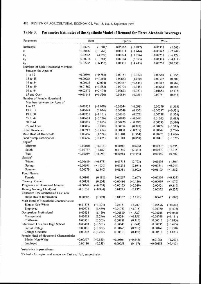
Although many of the household characteristic variables were significant, their impacts were typically small (Table 3). The demand for beer is affected positively by the number of male household members between the ages of 19 to 34, while the demand for wine is positively affected by the number of male household members between the ages of 50 to

64 and female members between the ages of 35 to 49. The benchmark household. which serves as a basis for consumption, lives in a rural area. is headed by a white male, has a female meal planner, is in the Income range of $30.000 to $50,000, is not a food-stamp participant. and lives in the East. Urban residents consume more wine, and families with a male head consume more spirits. Spirits consumption is higher in the winter and spring and for people in the South. Wine consumption is higher in the winter and beer consumption is higher in the summer. Professional males consume fewer spirits, and college-educated females tend to consume more wine than their less-educated cohorts. In general, the impact of education on beer consumption is not significant. The proportion of food expen- diture on away-from-home consumption has a significant negative impact on wine consumption at home. This effect may be explained by the fact that wine is often consumed when people eat out. Also, this result is consistent with the estimated effects of another variable, household size in 21-meal equivalents. When more meals are eaten at home, less wine is consumed. The Mills' ratios are significant in spirits and wine demands, indicating the necessity to correct the selection bias caused by zero consumption.

The control variable estimates for the synthetic model, and the likelihood values and elasticities for its nested models are given in Table 4. Note that ;i: 1s close to unity and A? is close to zero. The ratios of coefficients to standard errors ( t )are substantially greater than 2. The synthet~c model tends to have a CBS and AIDS (W-System) income term and a price term that is close to that of AIDS (W-System). A likelihood ratio test is used to test the nested models. Rotterdam and CBS are rejected by the synthetic model by a large margin. The AIDS (W-System) is also rejected by the synthetic system, but by a much smaller margin. The expenditure and own-price elasticities of the nested level Rotterdam, CBS, and AIDS (W-System) models are also presented in Table 4 for comparisons. Estimates from the AIDS (W-System) are similar to the those of the synthetic demand system.

486 REVIEW OF AGRICULTURAL ECONOMICS, Vol. 18, No. 3, September 1996

Table 3. Parameter Estimates of the Synthetic Model of Demand for Three Alcoholic Beverages

Parameters

Intercepts e e,I e,z e,; Numbers of Male Household Members

between the Ages of I to 12 13 to 18 19 to 34 35 to 49 50 to 64 65 and Over

Number of Female Household Members between the Ages of I to 12 13 to 18 19 to 34 35 to 49 50 to 64 65 and Over

Urban Residence Male Head of Household Food Stamp Participation Regionh

Midwest South West

Seasonh Winter Spring Summer

Food Planner Female

Tenancy: Owner Pregnancy of Household Member Having Nursing Child(ren) Consulted DoctorlDietician Last Year

about Health Information Male Head of Household Characteristics:

Ethnic: Non-White Employed

Occupation: Professional Management Craftsman

Education: Less than High School Partial College College Graduate

Female Head of Household Characteristics Ethnic: Non-White Employed

"t-statistics in parentheses

Beer Spirits Wine

0.03221 (1.601)"0.05562 (-2.81 7) 0.02331 (1.563) -0.00832 (-1.762) -0.01033 (-1.644) -0.00542 (-2.944)

0.02965 (4.592) -0.00724 (- 1.226) -0.0225 1 (-6.428) -0.0071 6 (-I ,281) 0.02104 (3.393) -0.01 328 (-4.414) -0.02255 (-6.455) -0.0 139 1 (-4.4 13) 0.03250 (10.532)

-0.00394 (-0.783) -0.00161 (-0.362) 0.00560 (1.255) -0.00984 (-1.366) 0.00643 (1.070) 0.00302 (0.502)

0.00433 (2.094) -0.00447 (-0.844) 0.004 12 (0.762) -0.01 562 (- 1.558) 0.00704 (0.948) 0.00664 (0.883) -0.02472 (-2.474) 0.00623 (0.767) 0.01853 (2.175) -0.01 645 (-1 3.56) 0.00884 (0.955) 0.0076 1 (0.843)

-0.00535 (-1.038) -0.00044 (-0.098) 0.00579 (1.3 15) 0.00048 (0.074) 0.00249 (0.435) -0.00297 (-0.53 1 )

-0.00751 (-1.151) 0.000 13 (0.022) 0.00738 ( 1.326) -0.00603 (-0.726) -0.00400 (-0.549) 0.01003 (1.415)

0.00075 (0.085) -0.00470 (-0.595) 0.00393 (0.5 10) 0.00036 (0.098) 0.00334 (0.391) -0.00429 (-0.5 15)

-0.00247 (-0.404) -0.001 3 1 (-0.277) 0.00347 (2.754) 0.00436 (1.524) 0.01401 (1.964) -0.00975 (-1.404)

-0.00666 (-0.475) 0.OllOl (0.858) -0.0041 0 (-0.327)

-0.0001 0 (-0.01 6) 0.00386 (0.696) -0.00376 (-0.695) -0.00777 (- 1,187) 0.01347 (2.341) -0.00570 ( - I .O 15) -0.00059 (-0.090) -0.00281 (-0.485) 0.00340 (0.602)

-0.00619 (-0.873) 0.01715 (2.723) 0.01096 (1.804) -0.0069 1 (- 1.030) 0.01232 (2.081) -0.0054 1 (-0.944)

0.00279 (2.340) 0.01381 (1.002) -0.01 103 (-1.582)

0.00101 (0.181) 0.00297 (0.607) -0.00399 (-0.833) 0.001 59 (0.204) -0.00480 (-0.156) -0.00039 (-1.077)

-0.00248 (-0.203) -0.00153 (-0.080) 0.00401 (0.3 17) -0.0 1657 (-0.934) 0.0 1245 (0.837) 0.00352 (0.237)

0.00685 (I ,389) -0.01362 (-3.1 52) 0.00677 (1.006)

-0.0 1575 (- 1.424) 0.02 15 1 (2.209) -0.00576 (-0.606) 0.00973 (1.469) -0.01 753 (-3.016) 0.00780 (1.475) 0.00838 (1.159) -0.008 10 (-1.820) -0.00028 (-0.045) 0.01013 (1.296) -0.00244 (-0.356) -0.00769 (- 1.151 ) 0.00331 (0.505) 0.00181 (0.315) -0.005 12 (-0.9 13)

-0.00403 (-0.501) 0.00743 (1.041) -0.00335 (-0.485) -0.OOOOl (-0.002) 0.00165 (0.276) -0.00162 (-0.280)

0.00202 2 (0.282) 0.003 13 (0.492) -0.0051 8 (-I .83 I)

-0.00577 (-0.550) -0.00504 (-0.548) O.Ol08i (1.203) 0.00130 (0.253) 0.00053 (0.1 17) -0.001 83 (-0.415)

"efaults for region and season are East and Fall. respectively.

U.S. CONSUMER DEMAND FOR ALCOHOLIC BEVERAGES Wang, Gao. Wailes. Cramer 487

Table 3, Cont'd. Parameter Estimates of the Synthetic Model of Demand for Three Alcoholic Beverages

Parameters

Education: Less than High School Partial College College Graduate

Household Size in 21-Meal Equivalents

Proportion of Away-from-Home Food Expenditure

Mills' Ratio

"t-statistics in parentheses

Beer S~iri ts Wine

-0.00138 (-0 2 -0.00225 (-0.320) 0.00343 (0.513) 0.00077 (0.128) 0.00036 (0.069) -0.001 13 (-0221)

-0.00808 (-I. 173) 0.001 39 (0.233) 0.00662 ( 1.942)

0.00522 (I ,337) 0.001 83 (0.536) -0.00705 (-2.113)

0.00952 (0.754) 0.01038 (0.945) -0.01 990 (-2.855) 0.00976 (1.655) 0.01491 (2.080) -0.02467 (-4.863)

Table 4. Control Variables, Likelihood Values and Elasticities for Nested Models

Rotterdam CBS Model AIDS Model Model Model

Control Variables hl 0.041

(0.012)"

1, 0.942 (0.0 10)

Log-Likelihood Value 1.35'1.54 1,743.61 3.341.22

Expenditure Elasticity Beer 1.0951 0.9913 1.0122

(0.0261) (0.0065) (0.0031)

Spirits 1.1956 1.0612 0.9644 (0.0635) (0.0234) (0.0105)

Wine 0.6101 0.9743 0.9947 (0.0552) (0.0101) (0.0072)

Own Compensated Price Elasticity Beer -0.5 166 -0.0953 -0.362 1

(0.0759) (0.0239) (0.0103)

Wine -0.9271 -0.0772 -0.6263 (0.1086) (0.0201) (0.0144)

"Standard errors in parentheses.

Summary and Conclusions

In first-stage budgeting, a double-hurdle model identifies two different decisions on whether to consume alcohol as well as how much. The decisions are made jointly, and a bivariate cumulative distribution function has to be numerically optimized to get estimates. Some household characteristic variables affect the decision on whether to consume but not on how much, while some affect the two decisions in an opposite way. A level version synthetic model is used in the second-stage budgeting and it fits the data better than its nested functional forms (Rotterdam, CBS, and AIDS). Synthetic models have fewer restrictions on functional form and provide more flexibility in fitting data than the more conventional flexible functional forms. Therefore, synthetic models should be more readily considered when specifying an empirical model of consumer behavior.

The consumption of alcoholic beverages is an important social and economic issue. Society wants to control alcohol consumption because of the health hazards, social problems, work ethic problems, and traffic hazards related with its misuse. On the other hand, the government generates substantial tax revenues from its sale. Reliable information on the nature of the demand for alcoholic beverages is, therefore, important in formulating optimal control. Household characteristic variables such as age, gender, urbanization, region, season, and employment, along with health information, play an important role in the demand for alcoholic beverages. These results suggest that the quality adjustment

488 REVIEW OF AGRICULTURAL ECONOMICS. Vol. 18. No. 3. September 1996

has a significant impact on the accuracy of price elasticity estimates, especially for spirits in this sample. This result is not surprising because quality varies in spirits more than in other alcoholic beverages.

The evidence presented by results of the two-stage budgeting model using alcohol expenditure data for at-home consumption indicate that as a revenue generator, increasing excise taxes on alcoholic beverages is feasible; however. these taxes are not necessarily reliable sources of revenue.

References

Anderson, R.W. "Perfect Price Aggregation and Empirical Demand Analysis." Econonietricu 47( 1979): 1209-30.

Aptech Systems, Inc. "Gauss Applications: Optimization." Maple Valley, WA. 1994.

Atkinson. A.B.. J. Gomulka, and N.H. Stem. "Spending On Alcohol: Evidence from the Family Expenditure Survey 1970 to 1983." The Economic Journal 100(1990):808-27.

Barten, A.P. "Consumer Allocation Models: Choice of Functional Forms." Mimeo. Catholic University of Leuven and CORE, December 1990.

, "Towards A Levels Version of the Rotterdam and Related Demand Systems." Contributions to Operations Research and Economics: The Tu'entieth ,4nniversa/? of CORE, ed. B. Comet and H. Tulkens, p. 441-65. Cambridge, MA: The MIT Press. 1989.

Blaylock, J.R. and W.N. Blisard "Wine Consumption by US Men." ,4pplied Economics 24(1993):645-5 I .

Blundell, R. and C. Meghlr. "Bivariate Alternatives to the Tobit Model." Journal of Econometrics 34(1986): 179- 200.

Bureau of Labor Statistics and Census. Current Population Survey. Washington, DC, various years

Chiang, J. and L.F. Lee. "Discrete/Continuous Models of Consumer Demand with Binding Nonnegative Con- straints." Journal of Econometrics 54( 1992):79-93.

Cox, T.L. and M.K. Wohlgenant. "Prices and Quality Effects in Cross-Sectional Demand Analysis." American Journal of Agricultural Economics 68(1986):908- 19.

Cragg, J.G. "Some Statistical Models for Limited Dependent Variables with Application to the Demand for Durable Goods." Econometrics 39(197 1 ):829-44.

Deaton, A. "Quality. Quantity, and Spatial Variation of Price." The Anirrican Economic Revieiv 78( 1988):4 18- 30.

Deaton A. and J. Muellbauer. "An Almost Ideal Demand System." The ,4merican Economrr Ret,reic 70(1980):3 17-28.

Edgerton, D. "Estimating Elasticities in Multi-Stage Demand Systems." Presented at the AAEA annual meeting. Baltimore, Maryland, August 10, 1992.

Gao, X.M.. E. Wailes, and G. Cramer. "A Microeconometric Model Analysis of U.S. Consumer Demand for Alcoholic Beverages." Applied Econontics 27( 1995):59- 69.

General Accounting Office (GAO). tv'utrition hf~~nitoring. Mismanagement of h'utrition S u w e ~ Hu.7 Retulted in Questiontrble Data. Washington. DC: RCED-9 1 - 1 17. 1991.

Gourieroux. C. and A. Monfort. "On the Problem of Missing Data in Linear Models." Review of Economic Studies 48(1981):579-86.

Grossman. bl.. J.L. Sindelar, J. Mullahy. and R. Anderson. "Alcohol and Cigarette Taxes." Journul o f Eco~zornic Perspectiver 7( 1993):2 1 1-22.

Heien. D. and G. Pompelli. "The Demand for Alcoholic Beberages: Econom~c and Demographic Effects." Southern Economic Journal 55( 199 1 ):759-70.

Heien, D. and C.R. Wessells. "Demand System Estimation With Microdata: A Censored Regression Approach." Journal of' Business and Economic Statistlet 8(1990):365-7 1.

Johnson. J.A., E.H. Oksanen. M.R. Veall and D. Fretz. "Short-Run and Long-Run Elasticities for Canadian Consumption of Alcoholic Beverages: An Error-Correction Mechanism1 Cointegration Approach." Revievv o/'Economics and Statistics 74(1992):64-74.

Jones. A. M. "A Note on Computation of the Double-Hurdle Model with Dependence with An Application to Tobacco Expenditure." Bulletin of Economic Research 44(1992):67-73.

Kawkani, N.C. "On the Bias in Estimates of Import Demands Parameters." International Economic Revievv 13(1972):59-69.

Keller, W.J. and J. Van Driel. "Differential Consumer Demand Systems." European Economic Revievv 27(1985):375-90.

Maclure. M. "Demonstration of Deductive Meta-Analysis: Ethnol Intake and Risk of Myocardial Infarction." Epidemiologic Revievv 15(1993):328-5 I.

i ~ ~ ~ i ~ ~

U.S. CONSUMER DEMAND FOR ALCOHOLIC BEVERAGES Vliang, Gao. Wa~les, Cramer 489

Moore, R.D. and T.A. Pearson. "Moderate Alcohol United States Department of Agriculture, Human Nutr~tion Consumption and Coronary Artery Disease: A Review." Information Service. Evaluation of ~Vonresponse I I I the Merficirle 65( 1986):242-67. ,Vutionvvide Food Consumption Survej, 19x7-XX

Washington. DC: NFCS Report No. 87-M-2. 1992. Newey. W.K. "A Method of Moments Interpretation of

Sequential Estimators." Economics Letters white, H. -A ~~~i~~~ ~ ~ ,,f ~~ i k ~ l i h ~ ~ d 14( 1984):201-07. Misspecified Models." Economet~.ii,tr48( 1980): 1-25

Omstein. S.1. "Control of Alcohol Consumption Through Price Increases." Journal of Studies on Alcohol 4 1(1980):807- 18.

You have printed the following article:

U.S. Consumer Demand for Alcoholic Beverages: Cross-Section Estimation of Demographicand Economic EffectsJirong Wang; X. M. Gao; Eric J. Wailes; Gail L. CramerReview of Agricultural Economics, Vol. 18, No. 3. (Sep., 1996), pp. 477-489.Stable URL:

http://links.jstor.org/sici?sici=1058-7195%28199609%2918%3A3%3C477%3AUCDFAB%3E2.0.CO%3B2-K

This article references the following linked citations. If you are trying to access articles from anoff-campus location, you may be required to first logon via your library web site to access JSTOR. Pleasevisit your library's website or contact a librarian to learn about options for remote access to JSTOR.

[Footnotes]

Perfect Price Aggregation and Empirical Demand AnalysisRonald W. AndersonEconometrica, Vol. 47, No. 5. (Sep., 1979), pp. 1209-1230.Stable URL:

http://links.jstor.org/sici?sici=0012-9682%28197909%2947%3A5%3C1209%3APPAAED%3E2.0.CO%3B2-G

Spending on Alcohol: Evidence from the Family Expenditure Survey 1970-1983A. B. Atkinson; J. Gomulka; N. H. SternThe Economic Journal, Vol. 100, No. 402. (Sep., 1990), pp. 808-827.Stable URL:

http://links.jstor.org/sici?sici=0013-0133%28199009%29100%3A402%3C808%3ASOAEFT%3E2.0.CO%3B2-I

Prices and Quality Effects in Cross-Sectional Demand AnalysisThomas L. Cox; Michael K. WohlgenantAmerican Journal of Agricultural Economics, Vol. 68, No. 4. (Nov., 1986), pp. 908-919.Stable URL:

http://links.jstor.org/sici?sici=0002-9092%28198611%2968%3A4%3C908%3APAQEIC%3E2.0.CO%3B2-I

http://www.jstor.org

LINKED CITATIONS- Page 1 of 3 -

Some Statistical Models for Limited Dependent Variables with Application to the Demand forDurable GoodsJohn G. CraggEconometrica, Vol. 39, No. 5. (Sep., 1971), pp. 829-844.Stable URL:

http://links.jstor.org/sici?sici=0012-9682%28197109%2939%3A5%3C829%3ASSMFLD%3E2.0.CO%3B2-K

Quality, Quantity, and Spatial Variation of PriceAngus DeatonThe American Economic Review, Vol. 78, No. 3. (Jun., 1988), pp. 418-430.Stable URL:

http://links.jstor.org/sici?sici=0002-8282%28198806%2978%3A3%3C418%3AQQASVO%3E2.0.CO%3B2-Q

An Almost Ideal Demand SystemAngus Deaton; John MuellbauerThe American Economic Review, Vol. 70, No. 3. (Jun., 1980), pp. 312-326.Stable URL:

http://links.jstor.org/sici?sici=0002-8282%28198006%2970%3A3%3C312%3AAAIDS%3E2.0.CO%3B2-Q

On the Problem of Missing Data in Linear ModelsChristian Gourieroux; Alain MonfortThe Review of Economic Studies, Vol. 48, No. 4. (Oct., 1981), pp. 579-586.Stable URL:

http://links.jstor.org/sici?sici=0034-6527%28198110%2948%3A4%3C579%3AOTPOMD%3E2.0.CO%3B2-H

Policy Watch: Alcohol and Cigarette TaxesMichael Grossman; Jody L. Sindelar; John Mullahy; Richard AndersonThe Journal of Economic Perspectives, Vol. 7, No. 4. (Autumn, 1993), pp. 211-222.Stable URL:

http://links.jstor.org/sici?sici=0895-3309%28199323%297%3A4%3C211%3APWAACT%3E2.0.CO%3B2-V

The Demand for Alcoholic Beverages: Economic and Demographic EffectsDale Heien; Greg PompelliSouthern Economic Journal, Vol. 55, No. 3. (Jan., 1989), pp. 759-770.Stable URL:

http://links.jstor.org/sici?sici=0038-4038%28198901%2955%3A3%3C759%3ATDFABE%3E2.0.CO%3B2-K

http://www.jstor.org

LINKED CITATIONS- Page 2 of 3 -

Demand Systems Estimation with Microdata: A Censored Regression ApproachDale Heien; Cathy Roheim WessellsJournal of Business & Economic Statistics, Vol. 8, No. 3. (Jul., 1990), pp. 365-371.Stable URL:

http://links.jstor.org/sici?sici=0735-0015%28199007%298%3A3%3C365%3ADSEWMA%3E2.0.CO%3B2-M

Short-Run and Long-Run Elasticities for Canadian Consumption of Alcoholic Beverages: anError-Correction Mechanism/Cointegration ApproachJames A. Johnson; Ernest H. Oksanen; Michael R. Veall; Deborah FretzThe Review of Economics and Statistics, Vol. 74, No. 1. (Feb., 1992), pp. 64-74.Stable URL:

http://links.jstor.org/sici?sici=0034-6535%28199202%2974%3A1%3C64%3ASALEFC%3E2.0.CO%3B2-C

On the Bias in Estimates of Import Demand ParametersN. C. KakwaniInternational Economic Review, Vol. 13, No. 2. (Jun., 1972), pp. 239-244.Stable URL:

http://links.jstor.org/sici?sici=0020-6598%28197206%2913%3A2%3C239%3AOTBIEO%3E2.0.CO%3B2-R

Maximum Likelihood Estimation of Misspecified ModelsHalbert WhiteEconometrica, Vol. 51, No. 2. (Mar., 1983), p. 513.Stable URL:

http://links.jstor.org/sici?sici=0012-9682%28198303%2951%3A2%3C513%3AMLEOMM%3E2.0.CO%3B2-S

http://www.jstor.org

LINKED CITATIONS- Page 3 of 3 -