Embed Size (px)
Citation preview
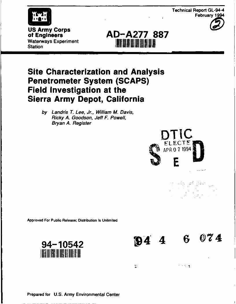
Technical Report GL-94-4February 1994*
US Army Corpsof Engineers AD-A277 887Waterways Experiment I IIl1Station 11iji l oll , 11111 Jil 11111 1
Site Characterization and AnalysisPenetrometer System (SCAPS)Field Investigation at theSierra Army Depot, California
by Landris T. Lee, Jr., William M. Davis,Ricky A. Goodson, Jeff F. Powell,Bryan A. Register
DTICEL.ECTF -APR 07 1994
Approved For Public Release; Distribution Is Unlimited
94-10542 4 4P IIrepared I IU , Am i r CIIIIn tII
Prepared for U.S. Army Environmental Center
The contents of this report are not to be used for advertising,publication, or promotional purposes. Citation of trade namesdoes not constitute an official endorsement or approval of the useof such commercial products.
PMDfIU ON RECYCLED PAEIR

D'ISCLAIMER NOTICE
THIS DOCUMENT IS BEST
QUALITY AVAILABLE. THE COPY
FURNISHED TO DTIC CONTAINEDA SIGNIFICANT NUMBER OF
COLOR PAGES WHICH DO NOT
REPRODUCE LEGIBLY ON BLACK
AND WHITE MICROFICHE.
Technical Report GL-94-4February 1994
Site Characterization and AnalysisPenetrometer System (SCAPS)Field Investigation at theSierra Army Depot, Californiaby Landris T. Lee, Jr., William M. Davis,
Ricky A. Goodson, Jeff F. Powell,Bryan A. Register
U.S. Army Corps of Engineers Accesion ForWaterways Experiment Station3909 Halls Ferry Road NTIS CRA&IVicksburg, MS 39180-6199 DTIC TAB
U, amnounced 0
B.................By .............. ........... ....... .........
Di t ibi-tion f
Availability Codest Avai! acd/or
Di Specit
Final reportApproved for public release; distribution is unlimited
Prepared for U.S. Army Environmental CenterAberdeen Proving Ground, MD 21010-5401

US Army Corpsof EngineersWaterways Experiment -Station riication Data
16 .il 8c.-(ehia repot ;GL-4-4
Eniomna Cne.N .. ryEgne Waterways= Exenen
WGlaI•AM L IOM1OM
WAT•OFRERWAYSON E04M.? IrATI
S.[tatio. ;. prepaes: Tehnca rpt(U.S. ArmyCrso Engineers Wt.wy
165 Experiment Station)chialort ;DGa-9ta-4
Includes biAliographical references.1. Oil pollution of, .c- Californi. 2. Penetrometer. 3. Rluodimetr.
I. Lee, Landris T. 1I. ,- 1 States. Army. Corps of Engineers. 1ll. U.S.Environmental Centei. ,4. U.S. Army Engineer Waterways ExpermentStation. V. Series: Technical report (U.S. Army Engineer WaterwaysExperiment Station) ; GL-94-4.TA7 W34 no.GL-94-4

Contents
Preface ... ........................................ vi
Conversion Factors, Non-SI to SI Units of Measurement ........... viii
1 -Introduction ....................................... 1
Overview ......................................... 1Objectives ......................................... 1
2-Site Description ..................................... 4
Physiography and Climate .............................. 4Geology and Hydrogeology .............................. 4Site History ........................................ 5
3-Investigation Equipment and Procedures .................... 10
General Operation ................................... 10Penetrometer Sensors and Data Collection ................... 12Support Systems .................................... 13Penetrometer Fluorescence Verification .................... 15
4-Results and Discussion ................................ 19
General .......................................... 19Soil Classification Measurements . ....................... 20Soil Fluorescence .................................... 29Support Systems .................................... 30Penetrometer Fluorescence Verification .................... 56
5-Summary, Conclusions, and Recommendations ................ 81
Bibliography ...................................... 86
Appendix A: Standard Practice for Preparation of Calibration SoilSamples for the SCAPS Laser-Induced Fluorescence Sensor ......... Al
Appendix B: Surveying Data . ........................... BI
Appendix C: SCAPS Field Sampling Standard Operating Procedure ... CI
Appendix D: Data Plots from Penetrometer Pushes .............. D1
Appendix E: Verification Sample Information .................. El
SF 298
III
Ust of Figures
Figure 1. Site map showing location of the Sierra Army Depot ..... 2
Figure 2. Geologic map of Honey Lake Valley ................ 6
Figure 3. Geologic cross section A-A' ...................... 7
Figure 4. Geologic cross section B-B' ...................... 8
Figure 5. Site map of the Diesel Spill Area ................... 9
Figure 6. The SCAPS truck ............................. 11
Figure 7. Pushpipe configurations ........................ 21
Figure 8. Site Map of the Diesel Spill Area Penetrations ......... 22
Figure 9. Penetration termination values .................... 25
Figure 10. X-ray diffraction pattern ......................... 28
Figure 11. Soil stratigraphy 3-D model visualization, View 1 ....... 31
Figure 12. Soil stratigraphy 3-D model visualization, View 2 ........ 33
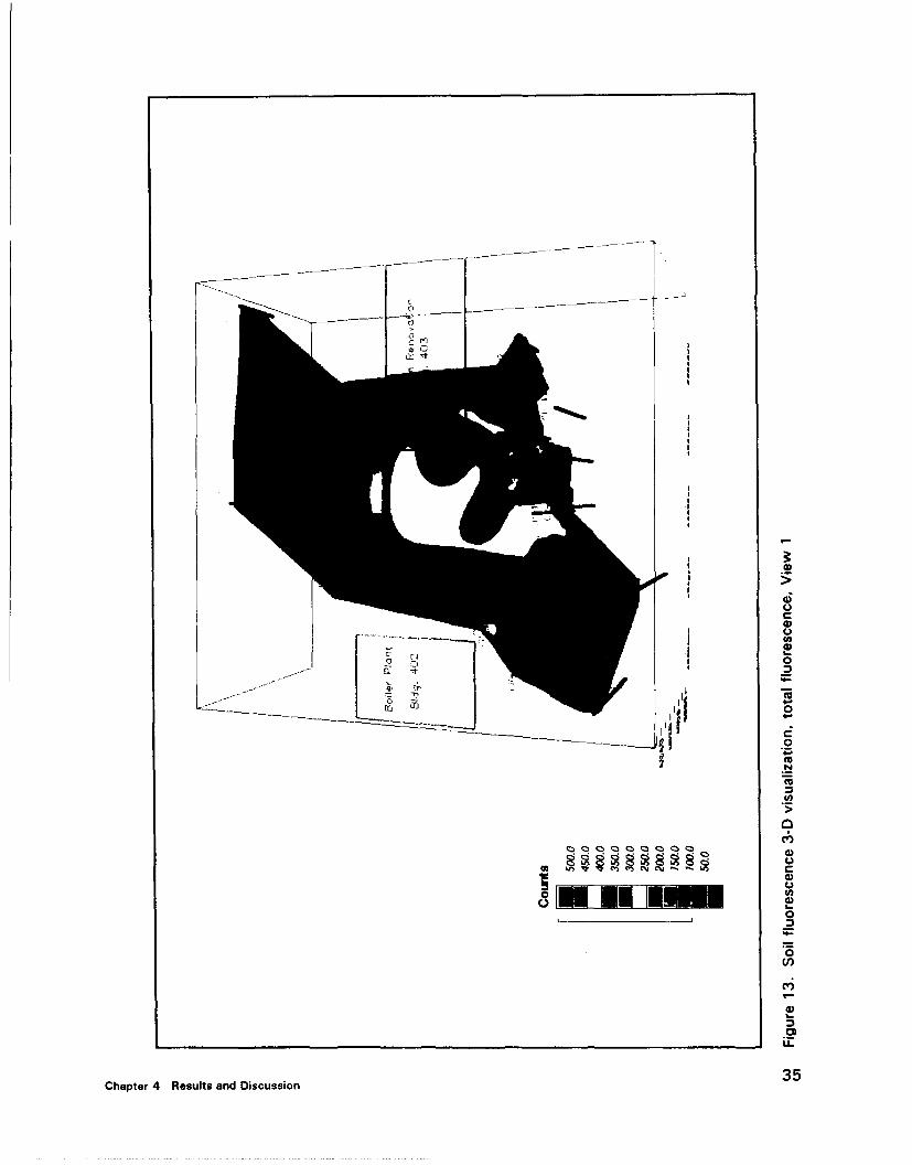
Figure 13. Soil fluorescence 3-D visualization,total fluorescence View I ....................... 35
Figure 14. Soil fluorescence 3-D visualization,total fluorescence View 2 ....................... 37
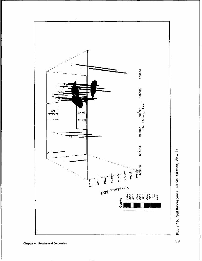
Figure 15. Soil fluorescence 3-D visualization, View la .......... 39
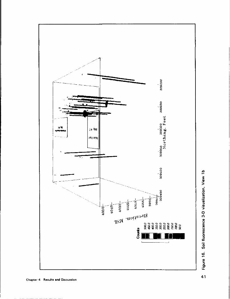
Figure 16. Soil fluorescence 3-D visualization, View lb .......... 41
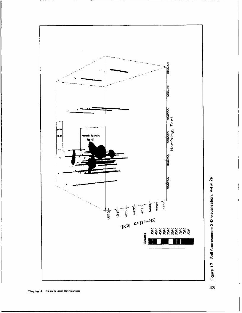
Figure 17. Soil fluorescence 3-D visualization, View 2a .......... 43
Figure 18. Soil fluorescence 3-D visualization, View 2b. .......... 45
Figure 19. Soil fluorescence 3-D visualization, View 3a .......... 47
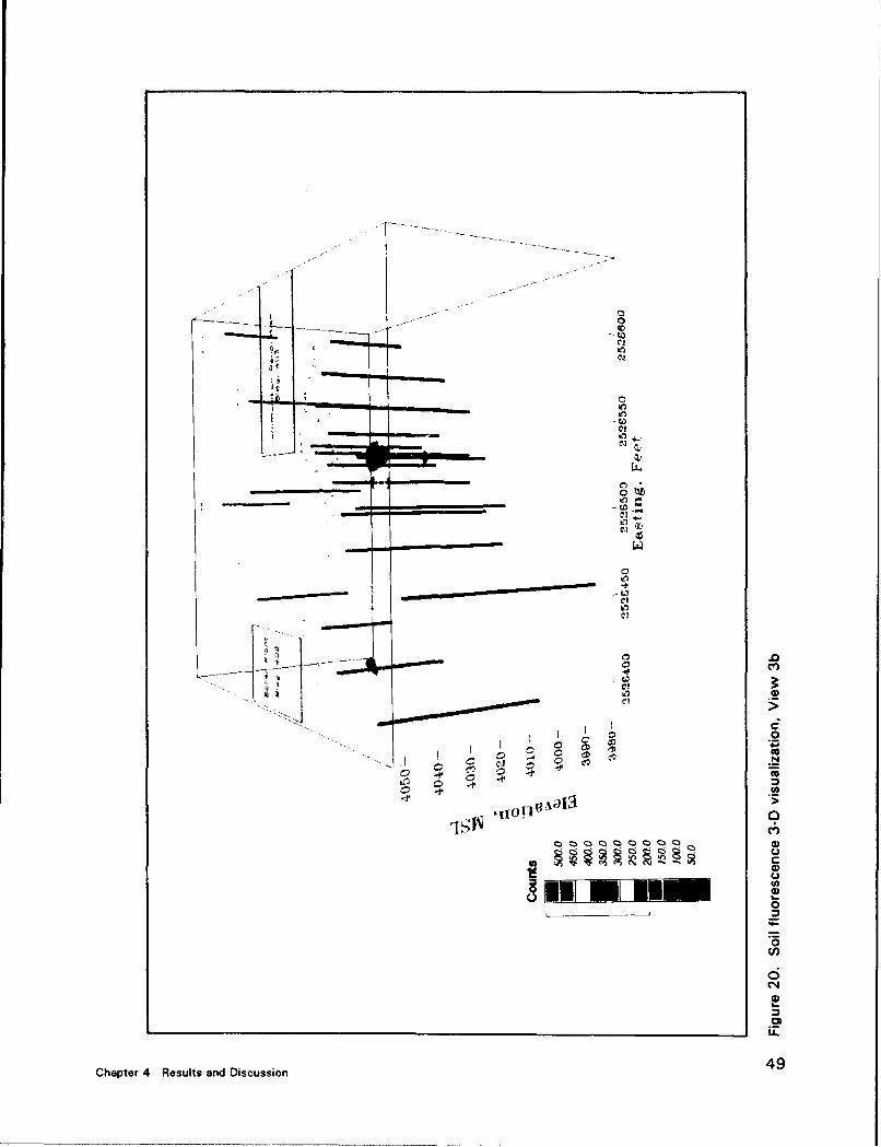
Figure 20. Soil fluorescence 3-D visualization, View 3b .......... 49
Figure 21. Soil fluorescence 3-D visualization, View 4a .......... 51
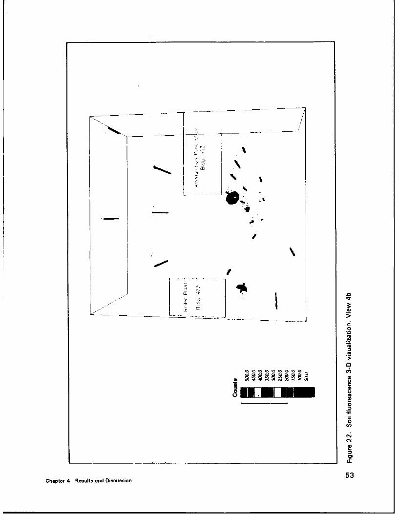
Figure 22. Soil fluorescence 3-D visualization, View 4b .......... 53
Figure 23. Sierra Native TRPH vs TPH ..................... 61
Figure 24. Sierra Native TRPH vs TPAH .................... 61
Figure 25. Sierra Native TPAH vs TPH ..................... 62
Figure 26. Sierra Fill TRPH vs TPH ....................... 62
Figure 27. Sierra Fill TRPH vs TPAH ....................... 63
Figure 28. Sierra Fill TPAH vs TPH ........................ 63
Figure 29. Native TRPH vs fluorescence ..................... 65
Figure 30. Native TPH vs fluorescence ...................... 65
iv

Figure 31. Native TPAH vs fluorescence ..................... 66
Figure 32. Fill TRPH vs fluorescence ....................... 66
Figure 33. Fill TPH vs fluorescence ........................ 67
Figure 34. Fill TPAH vs fluorescence ...................... 67
Figure 35. Horiba TRPH vs. EPA 418.1, field samples .......... 72
Figure 36. TPH vs TRPH, field samples ..................... 73
Figure 37. TPAH vs TRPH, field samples .................... 74
Figure 38. TPAH vs TPH, field samples ..................... 74
Figure 39. TRPH, Horiba vs fluorescence .................... 75
Figure 40. TRPH, EPA 418.1 vs fluorescence ................. 76
Figure 41. TPH vs fluorescence .......................... 77
Figure 42. TPAH vs fluorescence .......................... 77
Figure 43. Comparison of Fluorescence Emission Spectrafor Various Samples . ......................... 80
List of Tables
Table 1. Penetration points .............................. 23
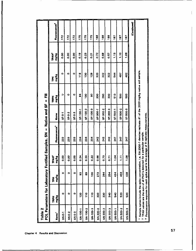
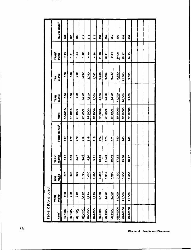
Table 2. POL Parameters for Laboratory Fortified Samples ........ 57
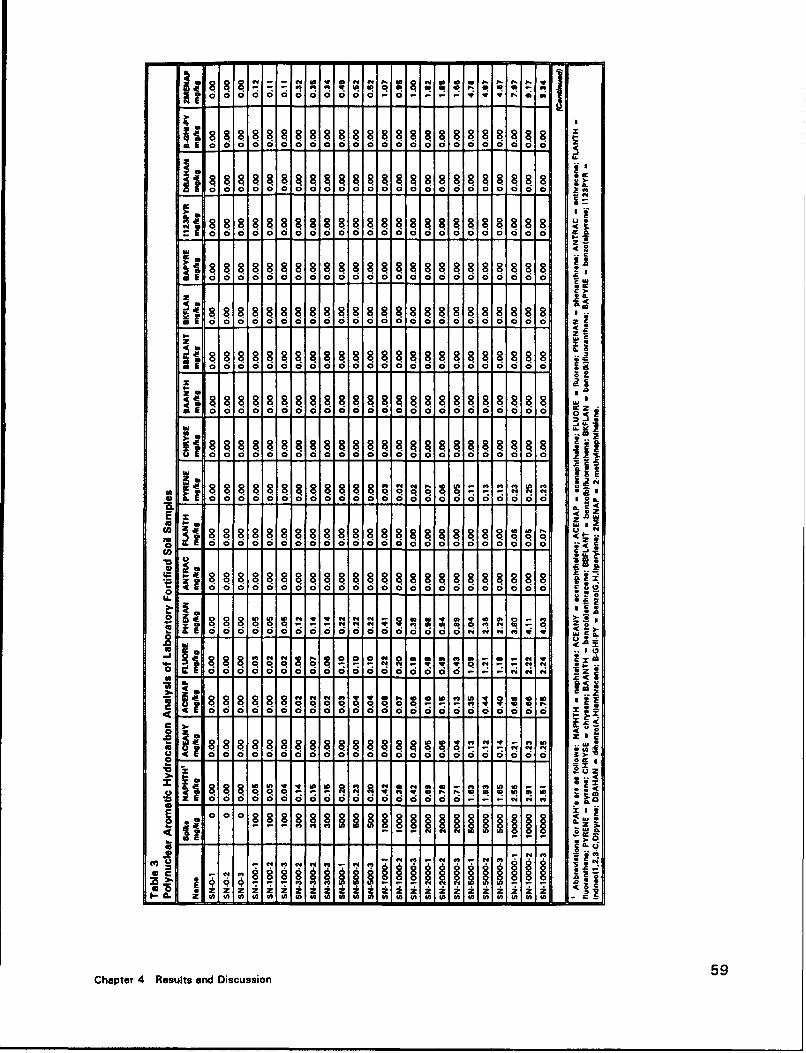
Table 3. Polynuclear Aromatic Hydrocarbon Analysis ofLaboratory Fortified Samples ...................... 59
Table 4. Sierra Army Depot Verification Samples POL Measures .... 69
Table 5. Polynuclear Aromatic Hydrocarbon Analysis ofField Soil Samples .............................. 70
Table 6. Comparison of Predicted POL Based on LaboratoryCalibration with Measured POL ..................... 78
V
Preface
The United States Army Engineer Waterways Experiment Station (WES)was tasked by the United States Army Environmental Center (AEC) to per-form Site Characterization and Analysis Penetrometer System (SCAPS) siteinvestigations at a designated location within the United States Army SierraArmy Depot (SIAD) near Herlong, California.
The AEC requested the WES to conduct SCAPS field investigations usingcone penetrometer-based sensors and samplers as screening-level tools in eval-uating the presence and location of suspected underground diesel fuel contami-nation at the designated Diesel Spill Area near Building 403 within theMagazine Storage Area. The field investigation was conducted in coordina-tion with the Department of Defense/AEC Installation Restoration ProgramSIAD contractor Montgomery Watson, Inc. The SCAPS field investigationwas conducted within the period of 28 September through 15 October 1993.
The AEC SCAPS Program Manager was Mr. George Robitaille, and theAEC SIAD Project Officer was Mr. Harry Kleiser. The SIAD Directorate ofEngineering and Housing Environmental Management Division Director wasMr. James Ryan, and coordination and helpful assistance was also provided bythat office's Mr. Bob Weis, Ms. Susan Holliday, and Mr. John Colberg.
The Montgomery Watson, Inc. Project Manager was Mr. Jerry Wickham.Site coordination and helpful assistance was provided by Mr. John Byrnes,Project Hydrogeologist, and Ms. Coleen Morf, Project Geologist.
The SCAPS field investigation was conducted by Messrs. Landris T.Lee, Jr., Karl F. Konecny, Geotechnical Laboratory (GL); Jeff F. Powell andBryan A. Register, Instrumentation Services Division (ISD); and Donald S.Harris, (Engineering and Construction Services Division). Field sample veri-fication analysis was conducted by Dr. William Davis, Mr. Roy Wade, andMr. Javier Cortes, Environmental Laboratory (EL).
Report preparation was done by Mr. Landris T. Lee, Jr., GL,Dr. William Davis, Mr. Ricky Goodson, EL, Mr. Jeff Powell, andMr. Bryan Register, ISD. Mr. J. D. Overton (Hilton Systems, Inc.) assistedwith data postprocessing, 3-D visualizations, and manning. Sample analyseswere performed by the Environmental Chemistry Braach, WES.Ms. Ann Strong supervised the analytical effort. The analysts included
vi
Mr. Richard Karn and Ms. Allyson Lynch (American Science InternationalCorporation). Mineral x-ray diffraction analysis was accomplished byMr. Jerry P. Burkes (Structures Laboratory). Soil index test analyses wereaccomplished in the GL's Soil Testing Facility, supervised byMr. Jessie Oidham.
The project was supervised by Mr. Joseph R. Curro, Jr., Chief, Engineer-ing Geophysics Branch, Mr. Mark Vispi, Chief, In Situ Evaluation Branch,Dr. A. G. Franklin, Chief, Engineering and Geosciences Division, andDr. W. F. Marcuson III, Director, GL. The project was under the manage-ment of Mr. John H. Ballard, Assistant Program Manager EL, Dr. JohnHarrison, Director, EL, and Dr. Jerome L. Mahloch, Program Manager,Executive Office.
At the time of publication of this report, Director of WES wasDr. Robert W. Whalin. Commander was COL Bruce K. Howard, EN.
vii

Conversion Factors,Non-SI to SI Units ofMeasurement
Non-SI units of measurement used in this document can be converted to SIunits as follows:
Multiply By To Obtain
acres 4,046.573 square meters
feet 0.3048 meters
gallons 3.785412 cubic decimeters
inches 2.54 centimeters
miles (U.S. statue) 1.609347 kilometers
pounds (mass) 0.4535924 kilogramstons (2,000 pounds mass) 907.1847 kilograms
VIIIm9k
1 Introduction
Overview
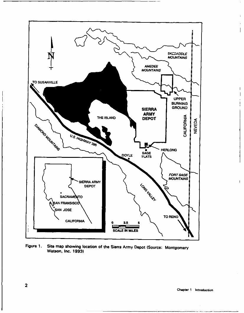
The United States Army Environmental Center (AEC) tasked the UnitedStates Army Engineer Waterways Experiment Station (WES) to perform sitecharacterization activities at a designated site within the United States ArmySierra Army Depot (SIAD). The SIAD is located in northern California, nearthe town of Herlong (Figure 1).
The Site Characterization and Analysis Penetrometer System (SCAPS) wasdeployed at SIAD from 28 September through 15 October 1993 (18 days).The deployment site was the Diesel Spill Area located adjacent t, Build-ing 403 within the Magazine Storage Area. Data from a total of 41 subsur-face penetration events (22 for sensing and 19 for sampling) were collectedduring this time period. The maximum depth achieved for data collectionpurposes was 70 ft below ground surface.
Objectives
There were five basic objectives for this site investigation. The first objec-tive was to collect sensing data from both the soil classification sensor and thefiber optic fluorometer (also referred to as the Laser-Induced Fluorometer, orLIF) sensor housed within the cone penetrometer probe. The soil classifica-tion sensor's purpose was to delineate the locations of subsurface stratigraphicchanges to enable a better understanding of the site geology. The fiber opticfluorometer sensor's purpose was to detect the presence of suspected subsur-face diesel fuel contamination adjacent to Building 403. The contaminantsource was a previous underground fuel line leak (Montgomery Watson, Inc.1993). A spatial extent determination of both the soil classification and con-tamination det( 'n data was possible by arranging the probe locations instrater;c patterns ' und the extent of the site.
A second objective was to collect samples of subsurface soil and water forsubsequent laboratoiy analysis to determine contaminant concentrations. Alimited set of soil and groundwater samples was obtained by pushing samplers
1Chapter 1 Introduction
TOSUSANVILLE
[ "q l SIERRA R UNoo
TH ISAN DEPO RONT;
1o
Figue 1 Sie mp sh win loatin o theSiera rmyDept (S urc: M ntg merWatso, Inc 1993
24Chpe& ntouto
housed within the cone penetrometer to various depths at selected locations onthe site.
The third objective was to conduct a robust verification of contaminantsensing capability as part of the ongoing SCAPS research and development.An onsite field-portable laboratory system was utilized to analyze retrievedsoil samples for contaminant concentration, and for direct comparison with thefiber optic fluorometer and soil classification sensor data.
The fourth objective was to continue the evaluation of the SCAPS demon-stration phase regarding the system capabilities. Identification of neededrefinements to the existing SCAPS system was an objective goal, and the dailyoperations provided additional experience in observing system performance.
The fifth objective was closely related to the fourth objective. Specifically,the field performance of the larger diameter (1.75 in.) pushpipe was evaluatedat this site.
3Chapter 1 Introduction
2 Site Description
Physiography and Climate
The SIAD is located in the broad Honey Lake Valley in the Basin andRange physiographic province. The Honey Lake Valley area has an extent of529 square miles within southeastern Lassen County, California. The HoneyLake Valley is bordered by northwest-trending mountains that rise 2,000 to3,000 ft above the valley floor. To the southeast are the Fort Sage mountains,to the northeast are the Skedaddle and Amedee mountains, and to the south-west are the Diamond mountains. The SIAD topography varies in elevationfrom 3,986 ft at Honey Lake level to approximately 4,134 ft above sea levelat Herlong. The surface relief does not vary appreciably within the SIADmain depot area (Montgomery Watson, Inc. 1993).
The surface environment consists mainly of sagebrush and low-lying desertvegetation. The climate is arid, and the average precipitation is only5.6 in./year U.S. Army Toxic and Hazardous Materials Agency(USATHAMA) (1979). During the period of this site investigation, rainfall inamounts up to approximately 1 in. were observed at the site. The rainfalloccurred during approximately 6 days out of 18. Daytime temperatures aver-aged approximately 70 °F, and nighttime temperatures often dipped to approx-imately 30 *F during the period.
Geology and Hydrogeology
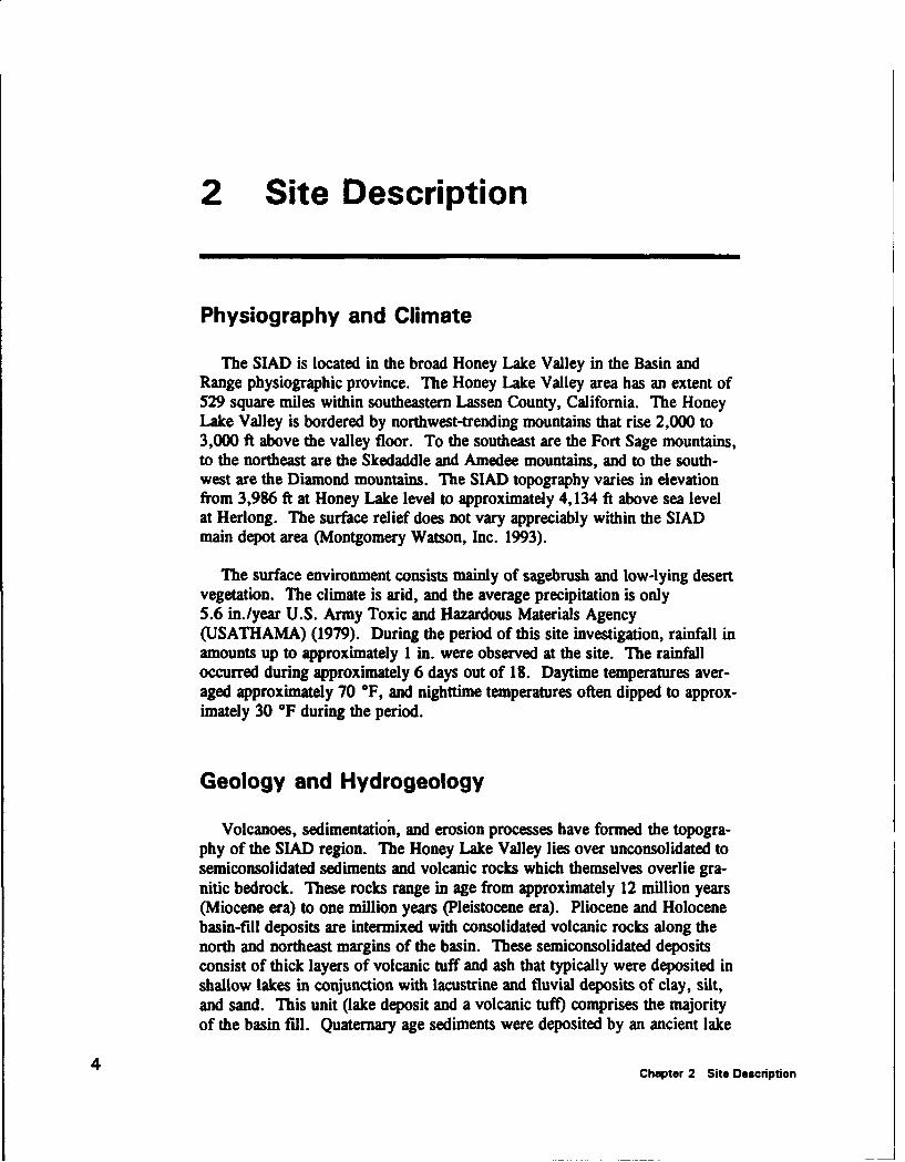
Volcanoes, sedimentation, and erosion processes have formed the topogra-phy of the SIAD region. The Honey Lake Valley lies over unconsolidated tosemiconsolidated sediments and volcanic rocks which themselves overlie gra-nitic bedrock. These rocks range in age from approximately 12 million years(Miocene era) to one million years (Pleistocene era). Pliocene and Holocenebasin-fill deposits are intermixed with consolidated volcanic rocks along thenorth and northeast margins of the basin. These semiconsolidated depositsconsist of thick layers of volcanic tuff and ash that typically were deposited inshallow lakes in conjunction with lacustrine and fluvial deposits of clay, silt,and sand. This unit (lake deposit and a volcanic tuft) comprises the majorityof the basin fill. Quaternary age sediments were deposited by an ancient lake
4 Chapter 2 Site Description
of which Honey Lake is a remnant. Sands and gravels predominate in thesesediments (Handman, Londquist, and Maurer 1990). Figures 2, 3, and 4depict the site geology. The surface soil in the general vicinity of the DieselSpill Area consists of the Amedee loamy sand series (Benioff, Filley, and Tsai1988). Between ground surface and 40 ft, the soil type is generally lightbrown, fine- to medium-grained, and well-sorted sand. Silts and claysinterbedded with sands are typical from approximately 40 to 120 ft belowsurface.
The surface soil in the Diesel Spill Area has been modified during recentbuilding construction, but originally consisted of the Preston sands. ThePreston sands are loose sands which are generally uniform to a depth of 6 ftor more. The texture is subject to considerable variation, and may contain anappreciable amount of fine material which has been windblown, giving it asandy loam texture (U.S. Department of Agriculture) (USDA) (1917).
Honey Lake is the prominent surface water feature in the basin. It has asurface area of approximately 47,000 acres and is fed intermittently frommore than 40 surface streams during snowmelt and infrequent rain events.The predominate groundwater flow pattern is toward the lake. In the DieselSpill Area (Figure 5), the groundwater flow is primarily northwards at anaverage gradient of approximately 0.003, and localized gradients range from0.001 to 0.01. The observed groundwater level in this area (from wellsDSA-02-MWA and DF-01-MWA) is approximately 62 ft below ground sur-face and is unconfined (Montgomery Watson, Inc. 1993).
Site History
The site history of SIAD precedes World War H, when Honey Lake wasused as a bombing range. In 1942 the Sierra Ordnance Depot wasconstructed. Several buildings and barracks have been added in subsequentyears. The current mission of the SIAD is to receive, stockpile, maintain, andissue muntions, strategic materials, and war reserve material(USATHAMA 1979).
At the Diesel Spill Area, a leaking diesel fuel pipeline at the southwestcorner of Building 403 was discovered on 3 March 1987. The pipeline ranunderground between a tank south of Building 402 (Boiler Plant No. 3) and aboiler in Building 403. Approximately 5,000 gal of diesel was estimated tohave been leaked prior to discovery. The underground storage tank has sincebeen removed, and the spill area was excavated and backfilled with clean soilin 1987. Remnant soil is contaminated with diesel-related compounds (Mont-gomery Watson, Inc. 1993).
Two monitoring wells have been installed in the Diesel Spill Area. WellDF-01-MWA was installed by USAEHA, and well DSA-02-MWA wasinstalled in 1991 by Montgomery Watson, Inc. During the groundwater
5Chapter 2 Site Description
..- .. . ...... .
... ... ............
..................
=31INT *d
CRE~~~b~~EOUONE ARNCBDOKU
Figure . Geolgic mapof Hony Lake alley SouRceR otoerAasn Ic 93
sapln peio of19 houh19,fur onsosmlswreaayefro eahoPhs el.TtlPtOlemHdoabnTP-isl a
deEctENDinoloeoftewls(F0- )atalvloaprim ey250CEN part pLISOErE milo % jp) %P iee wa no deete elwa 3etho
BAI-FL SEIETR in OST a olbrn S.0 B(proiaey2 tws fwlPLITOEE- PLICEN WOLA). RCSic nodtcal% ocnrtoso P-islwr on
iLOC NE SEIEThe Y AoNgrDietwl S- ti rsmdta h islcn
WatsonA Inc 1993)
6AE Chapte 2AL Site4 Descrptio

SOUTH NORTHA A'8,000
Siskeadde Mountains
TAW• " "' " ...... .
C,000
6 ,000 -,.,.-,,.
Hmy L@M Vdm _______
4AW.
"'""""2,0 ..: "" •: ••••.' . "••:•••-_-••-.•-------'---•. ---- --- ••
%. % -.- ----..---.-.. . ..----- . =:-..--- : .
SEA LEVEL .' . .IAN • , ,
LEGEND
H__ OL OCENE AND PLEISTOCENE BASN- 1~PLIOCENE SEDSWENTARY AN SCALE IN MILESFILSEDP&EITARY OEPOS(TS PYOLSI DEPOSITS
0 U £'"MIOCENE TO OLIGOCENE _______RArI BDOK ETCA XGGRTONX1VOLCANIC ROCKS A COSOATCSmCVEICLAGRAOHXC
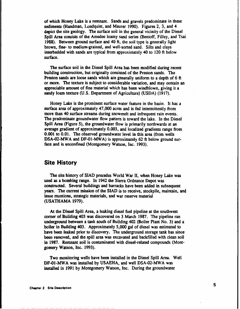
Figure 3. Geologic cross section A-A' (Source: Montgomery Watson, Inc. 1993)
7Chapter 2 Site Description

WEST EAST
* am
IAN IAN
LEN
LEGEND
_____ CWCNE AMQPLESTOC84 SAEN-jf PI.=8E SEDVWBETARY r--vff4Utd LE3FLL EDIETARYOEJOS*T I PYtdOO.ASTIC DEPOSJTS M "
0 aI
VOLCAMC OW=W
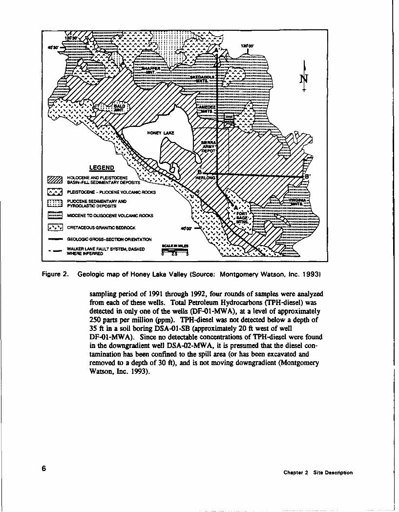
Figure 4. Geologic cross section B-B' (Source: Montgomery Watson, Inc. 1993)
8 Chopter 2 Site Description

CoFint mintew Shopa
Figure 5.S(Veitle m ap ofthnne Dieae) pl ra(ouc:Mngmr WtoIc93
Chpe 2ole Plate jDeORrSOPtROA
3 Investigation Equipment andProcedures
General Operation
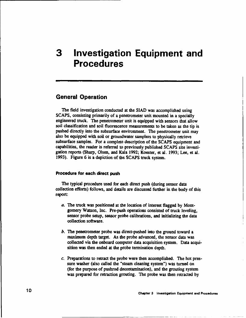
The field investigation conducted at the SIAD was accomplished usingSCAPS, consisting primarily of a penetrometer unit mounted in a speciallyengineered truck. The penetrometer unit is equipped with sensors that allowsoil classification and soil fluorescence measurements to be taken as the tip ispushed directly into the subsurface environment. The penetrometer unit mayalso be equipped with soil or groundwater samplers to physically retrievesubsurface samples. For a complete description of the SCAPS equipment andcapabilities, the reader is referred to previously published SCAPS site investi-gation reports (Sharp, Olsen, and Kala 1992; Koester, et al. 1993; Lee, et al.1993). Figure 6 is a depiction of the SCAPS truck system.
Procedure for each direct push
The typical procedure used for each direct push (during sensor datacollection efforts) follows, and details are discussed further in the body of thisreport:
a. The truck was positioned at the location of interest flagged by Mont-gomery Watson, Inc. Pre-push operations consisted of truck leveling,sensor probe setup, sensor probe calibrations, and initializing the datacollection software.
b. The penetrometer probe was direct-pushed into the ground toward amaximum depth target. As the probe advanced, the sensor data wascollected via the onboard computer data acquisition system. Data acqui-sition was then ended at the probe termination depth.
c. Preparations to retract the probe were then accomplished. The hot pres-sure washer (also called the "steam cleaning system") was turned on(for the purpose of pushrod decontamination), and the grouting systemwas prepared for retraction grouting. The probe was then retracted by
10 Chapter 3 Investigation Equipment and Procedures
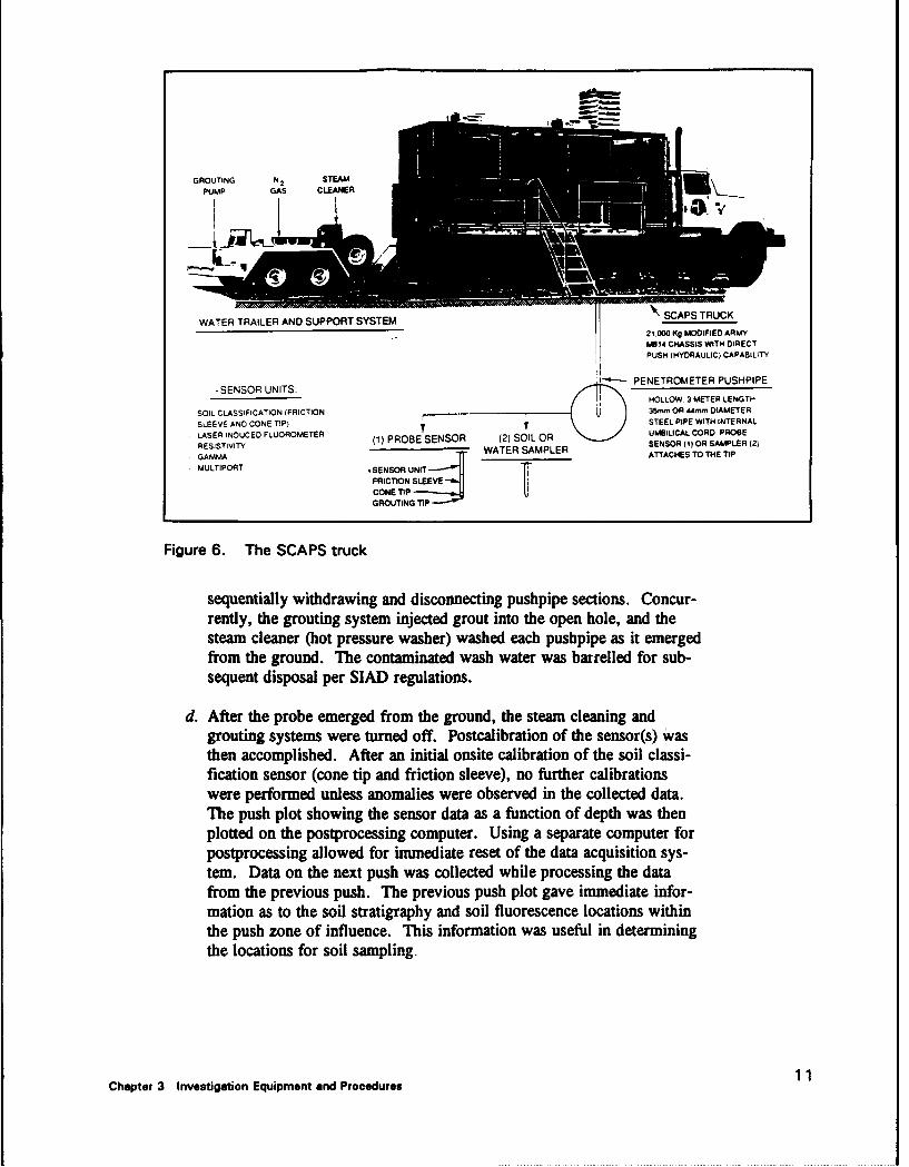
GROUTING N2 STEAMPUMP GAS CLEANE¢R
WATER TRAILER AND SUPPORT SYSTEM SCAPS TRUCK
21.000 Kg MODIFIED ARMYM814 CHASSIS WITH DIRECTPUSH (HYDRAULIC) CAPABILITY
SES T -PENETROMETER PUSHPIPE-SENSOR UNITS:
HOLLOW, 3 METER LENGTH
SOIL CLASSIFICATION (FRICTION 35rm OR 44mm DIAMETER
SLEEVE AND CONE TIP) STEEL PIPE WITH INTERNAL
LASER INDUCEO FLUOROMETER UMBILICAL CORD PROBERESISTIVITY (1) PROBE SENSOR (2) SOIL OR SENSOR (1) OR SAMPLER (2)RESISIVIT TER OSASMPLEER
GAMMAWATER SAMPLER ATTACHES TO THE TIP
. MULTIPORT -SENSOR UNIT
FRICTION SLEEVECONE TIPGROUTING TiP
Figure 6. The SCAPS truck
sequentially withdrawing and disconnecting pushpipe sections. Concur-rently, the grouting system injected grout into the open hole, and thesteam cleaner (hot pressure washer) washed each pushpipe as it emergedfrom the ground. The contaminated wash water was barrelled for sub-sequent disposal per SIAD regulations.
d. After the probe emerged from the ground, the steam cleaning andgrouting systems were turned off. Postcalibration of the sensor(s) wasthen accomplished. After an initial onsite calibration of the soil classi-fication sensor (cone tip and friction sleeve), no further calibrationswere performed unless anomalies were observed in the collected data.The push plot showing the sensor data as a function of depth was thenplotted on the postprocessing computer. Using a separate computer forpostprocessing allowed for immediate reset of the data acquisition sys-tem. Data on the next push was collected while processing the datafrom the previous push. The previous push plot gave immediate infor-mation as to the soil stratigraphy and soil fluorescence locations withinthe push zone of influence. This information was useful in determiningthe locations for soil sampling.
11Chapter 3 Investigation Equipment and Procedures

Procedure for obtaining physical samples
The typical procedure used for obtaining physical samples follows:
a. The truck was positioned near a previous push point where sensor datahad been collected. This procedure was f, .1owed in order to obtainrepresentative samples from depths corre.-onding to the adjacent sensorprobe push. In most cases, the sample ,,cation was within 1 to 2 ft ofthe original sensor push point. A clos-r location was not desired sincethe original sensor push point hole had been grouted, and samplesinfluenced by the grout material were not desired.
b. The sampler was attached to the empty pushpipe (no umbilical cord wasneeded) and was hydraulically pushed 4irectly into the ground in thesame fashion as the sensor probe. The data acquisition computer sys-tem was utilized only to provide a depth display as the pushpipe waspushed to depth. At the target depth, the sampler was mechanicallyactivated and a sample (soil or groundwater) was physically retrieved.
c. The sample was brought to the surface by sequentially retracting thepushpipe sections. The steam cleaning system (hot pressure washer)was used for pushpipe decontamination. At the surface, the sample wasremoved from the sampler and placed in the appropriate container forsubsequent analysis and/or shipment. No retraction grouting was donedue to the absence of the internal umbilical cord containing the grouttube. Manual grouting was performed by pouring the grout mixturedown the open hole.
Penetrometer Sensors and Data Collection System
Penetrometer investigations at this site were performed utilizing two sen-sors: the soil classification sensor and the soil fluorescence sensor (LIF).Signal conditioning, data acquisition, and data processing constituted the datacollection system that was employed with the sensors.
The soil classification sensor consists of se-: rate electro-mechanical strain-gauged elements within the cone tip and the cL,:Ie friction sleeve. Theelements' responses to external soil stresses constitute the typical electricalcone penetrometer probe configuration for soil stratigraphy identification andsubsequent classification. The reader is referred to previous SCAPS reportsfor a detailed explanation of the soil classification system (Sharp, Olsen, andKala 1992; Koester et al. 1993, Lee, et al. 1993). Typically, the twoelements sense the changes in soil stresses as the probe is pushed to depth.The electro-mechanical responses are translated into Soil ClassificationNumbers (SCN via the computerized data collection system. Each SCN rep-resents a soil type which corresponds to elementary soil classificationdescriptions (sand, silt, clay, etc.). The two elements (cone tip and friction
12 Chapter 3 Investigation Equipment and Procedures
sleeve) independently respond to soil stresses, but the combined responsecontributes to the development of the SCN.
LIF consists of an onboard laser system pulsing ultraviolet light throughoptical fibers in the pushpipe umbilical cord, terminating in a 6.35 mm-diamsapphire window on the penetrometer probe. As the probe advances, the firedultraviolet light (wavelength of 337 nanometers (rnm)) pulses emanate throughthe window into the soil. The soil matrix reacts to the pulsed light, and theresponse signal (light) is returned through the window and a separate opticalfiber up to an onboard optical analyzer. The return signal characteristics(peak wavelength and intensity) indicate the nature of fluorescent materials inthe soil matrix. Since most hydrocarbon contaminants (diesel, oils, etc.)fluoresce under these conditions, the presence or absence of those contami-nants is determined. In addition, the relative concentration levels of thosecontaminants may be ascertained when additional calibrations are performed.The fluorometer probe was attached to both the larger diameter (1.75 in.)pushpipe and the smaller diameter (1.4 in.) pushpipe at separate times duringthis investigation. The larger diameter pushpipe configuration had not beenutilized during a site investigation prior to the SIAD site investigation. Dis-cussions of the configurations used at the SIAD are detailed later in the bodyof this report.
The computerized data collection system is integral to all sensor systems.During the penetration event, it allows for real-time sensor performance evalu-ation and data acquisition. The "raw" signals acquired via the sensors aredisplayed on the computer monitors as the probe advances into the soil. Thequality of the penetration event is assured, preventing unnecessary or errone-ous data collection. After each penetration event, the data collected during theevent is automatically distributed to appropriate data files for subsequentpostprocessing and plotting as needed. The generation of three-dimensional(3-D) descriptions of acquired site data is integral to the postprocessingfunction, and is presently performed at WES after the field investigation iscompleted.
Support Systems
The support systems include auxiliary components of SCAPS not directlyidentifiable with the sensors or data collection system but required to make theSCAPS fully functional. These include site surveying, surface geophysics(locating buried utilities and other obstructions), soil and groundwater sam-pling, pushpipe decontamination, grouting, and other items necessary to com-plement the overall performance.
Surveying and geophysics
The site surveying and geophysics were accomplished at this site as atother sites, with the exception that the role of geophysics by SCAPS was less
13Chapter 3 Investigation Equipment and Procedures
prominent at the SIAD. The equipment and methods used for surveying andgeophysics were similar to those used at previous sites (Sharp, Kala, andPowell 1992; Koester, et al. 1993a; Lee, et al. 1993). The SIAD providedunderground utility location assistance to prevent disruptive outages of nearbyelectrical feeds and fuel lines caused by accidental penetration. SCAPS geo-physics was limited to determining locations of any other possible under-ground obstructions.
Grouting
Grouting was performed to ensure that vertical cross contamination did notoccur in the penetration holes. To accomplish this goal, a grout mixtureconsisting of Portland cement (Basalite" brand), potable water, and sodiumBentonite was either automatically pumped into the hole as the penetrometerprobe was retracted or manually placed into the hole after the sampler probewas withdrawn. In an attempt to achieve a grout mixture which met theregulatory requirements as closely as possible, yet be pumpable through the3/8-in.-diam umbilical cord grout tube, several mixtures were tried. Theaccepted State of California grout mixture consists of one bag of Portlandcement, 7 to 8 gal of potable water, and 5 percent Bentonite by weight. Therequired grout mixture consisted of 3 parts of cement to 2 parts of water byweight plus 5 percent Bentonite. The viscosity of this mixture was too highfor adequate pumpability. The amount of Bentonite was reduced to approxi-mately 2 percent by weight, and the mixture was pumpable, although frequentcleaning of the umbilical cord grout tube was required to prevent clogging.Tacit approval was given for this mixture, primarily due to the innovativetechnology being demonstrated. During physical sampling operations, thegrout mixture (with 5 percent Bentonite) was manually placed in the openpenetration hole after retraction since no umbilical cord grout tubearrangement was possible when using either the soil or water sampler (neithersampler accommodates an umbilical cord).
Soil and groundwater sampling
Both soil and groundwater samples were retrieved during this investigation.For soil sampling, both the Goudae (now available through Hogentogler, Inc.,Columbia, Maryland) and Mostap" (A. P. van den Berg, Heerenveen, Neder-land) samplers were used interchangeably. For groundwater sampling, theHydropunch' (QED Groundwater Specialists, Ann Arbor, MI) Models Iand HI were used.
The Gouda' sampler was utilized to obtain the soil samples for Montgom-ery Watson, Inc. It has an OD of approximately 1.75 in. and retrieves a sam-ple of approximately 1-in. diam by 8-in. length (approximately 100 cm3
internal volume). It was connected to the smaller diameter (1.4 in.) pushpipe,and consists of a stab-type sampler which is mechanically activated by retract-ing the pushpipe string 10.5 in. and then pushing the extended sampler a
14 Chapter 3 Investigation Equipment and Procedures
distance of 9.5 in. The soil is forced into the sampler tube over a depth inter-val of 8 in.
The Mostap'T 35 sampler is a larger sampler (approximately 2-in. OD by24-in. length) which retrieves a sample of approximately 1.5-in. diam by18-in. length (approximately 550-c n3 internal volume). It is also a stab-typesampler, but is mechawically activated by releasing the tip and pushing thetube past the tip, forcing the soil into the sampler over the 18-in. depth inter-val. It was interchangeably connected to both pushpipe sizes (1.4 in. and1.75 in.), but was primarily used with the smaller diameter pushpipe. It wasutilized to obtain soil sampies for the penetrometer fluorometer sensor verifi-cation from the shallower depths where soil fluorescence had been observed(less than 20 ft).
The HydropunchTM Models I and II were used for the purpose of obtaininggroundwater samples. Both tools basically operate the same, by collectingin situ groundwater under hydrostatic pressure. The Model I collects approxi-mately 500 ml of water, and the Model II collects approximately 1 I of waterafter being mechanically opened at depth (more than 5 ft below the watertable). Both models are approximately 5 ft in length, but the Model I has aslightly smaller diameter than the Model I1. One important distinctionbetween the two models is that the Model II tip releases and remains in thehole after the sampler is retracted. It is thus not possible to obtain a deeperwater sample from the same penetration hole. Both the smaller and largerdiameter pushpipes were interchangeably used with the groundwater samplersat this site.
Penetrometer Fluorescence Verification
Laboratory calibration studies
Prior to the SCAPS truck deployment at SIAD, two uncontaminated soilsamples (approximately 10 kg each) were obtained from the area at SIAD thatwas to be investigated. The samples were obtained by the AEC project offi-cer from both an undisturbed area (Native SIAD) and an area where POL(diesel) contaminated soil had been excavated and the area backfilled (FillSIAD). These samples were shipped to WES Environmental ChemistryBranch (ECB) and were fortified with diesel fuel at varying concentrations.The procedure used to fortify soil samples with petroleum, oil, and lubricant(POL) contaminants has been developed by WES ECB and is described indetail in Appendix A.
Soil samples were fortified at 100, 300, 500, 1,000, 2,000, 5,000, and10,000-mg diesel fuel/kg dry weight soil. All soil samples fortified withdiesel fuel were analyzed for petroleum contamination by the methodsdescribed below:
15Chapter 3 Investigation Equipment and Procedures

Analyte Method
TRPH Method 418.1/9073
TPH EPA Method 8015
PAH's EPA Method 8270
TRPH refers to total recoverable petroleum hydrocarbons, TPH refers to totalpetroleum hydrocarbons and PAH's refer to polynuclear aromatic hydrocar-bons. It should be noted that the TPH measurements were made using thediesel fuel that was used to fortify the samples as the calibration standard forEPA Method 8015. The samples were also analyzed using the SCAPS POLsensor to determine the fluorescence response. The procedure consisted oftriplicate fluorescence analysis of each fortified soil sample pressed against thewindow of the POL sensor probe. The data obtained from these analyseswere used to develop laboratory calibration curves between the various mea-sures of POL contamination and the LIF response.
Field soil sampling
The purposes of the verification soil sampling phase of the SIAD fieldinvestigation were multifold:
a. An investigation of the utility of a field portable TRPH instrument foronsite verification of POL contamination identified by the SCAPS POLsensor.
b. A collection of soil samples for laboratory analysis to verify POL con-tamination identified by the SCAPS POL sensor.
c. An investigation of the feasibility of onsite POL sensor calibration withactual field contaminated soil samples using a field portable TRPHinstrument.
Sampling sites for verification sampling were chosen based on previousSCAPS penetrations that had indicated LIF response at a particular depth.Soil sampling locations were generally I to 2 ft offset from the conepenetrometer push site of interest. Soil samples collected adjacent to a partic-ular cone penetrometer push were denoted by prefixing the penetrometer pushname with S (for soil). Thus, soil sample SCP-14-1 denotes the first soilsample obtained from sampling at a particular depth adjacent to cone penetra-tion 14 (CP-14) (Appendix B). Samples were chosen based on a wide rangeof fluorescence response to provide a range of TRPH contaminated soil sam-ples. The wide range of POL contamination was desired to investigate theperformance of the field portable TRPH instrument for both POL verificationand potential calibration of the POL sensor in the field.
Field sampling procedures are determined by the EPA analytical methodsused to determine the concentration of the analytes of interest. The EPA soil
16 Chapter 3 Investigation Equipment and Procedures

sampling protocols for the analytes of interest were followed at SIAD and aredescribed in detail in the WES SCAPS Field Sampling Standard OperatingProcedure (Appendix C). This procedure is excerpted from the "OperationsManual for the Site Characterization and Analysis Penetrometer System"(Koester et al. 1993b). Samples were collected using the Mostap soil sampl-ing device pushed to depth using the SCAPS truck. Samples obtained in thismanner were homogenized in the field (mixed in a clean stainless steel panwith a stainless steel spatula) and placed in 500-mt widemouth jars withTeflon-lined lids. Although not part of the sampling Standard OperatingProcedure, homogenization was necessary for the field analysis for TRPHdiscussed below. These samples were analyzed in the field for TRPH and LIFas described below. The samples were then shipped to the WES ECB forTRPH (EPA Method 418.1), TPH (EPA Method 8015), and TPAH (EPAMethod 8270) analysis.
LIF determination and field total petroleum hydrocarbon
Fluorescence emission spectra of the homogenized soil samples wereobtained in the field by pressing the soil against the sapphire window of theSCAPS POL probe and collecting 10 replicated emission spectra. These10 replicate measurements were averaged. This procedure was carried out intriplicate for each soil sample investigated. The standard operating procedurefor the POL sensor operation includes analysis of rhodamine fluorescence dyeimmediately before and after each cone penetrometer push. This is accom-plished by placing a cuvette containing the rhodamine dye solution in front ofthe sapphire window, recording 10 spectra and averaging these spectra. Therhodamine dye spectra are used to normalize the penetrometer push fluores-cence data for any spectrometer system variation during a particular push. Asimilar procedure was used for the fluorescence emission spectra collected forthe homogenized soil samples. Before and after each fluorescence analysis ofa soil sample, triplicate measurements were made of the rhodamine dye solu-tion. These data were used to normalize the LIF response obtained for thesoil samples relative to the rhodamine response.
Field determination of the TRPH contamination of the homogenized soilsamples was carried out using a Horiba Model OCMA 220 TRPH analyzer.This instrument is a field portable fixed wavelength (3.4-3.5 microns,3,000 to 2,850 cma1) infrared detector designed to measure TRPH contamina-tion in water. A procedure was used to adapt the instrument for use as adetector for hydrocarbons contained in solvent extracts of soil. Ten grams ofsoil (wet weight) were weighed (electronic balance, accurate to 0.001 g) into a250 mf jar equipped with a Teflon-lined cap (1-Chem #320-0250). Twograms anhydrous Na2SO 4 were added to the soil and the sample was thor-oughly mixed using a stainless steel spatula. Two grams of silica gel (60-80mesh) were added to the soil and it was again mixed with a stainless steelspatula. Fifty ml of solvent (Flon-316) was added and the mixture wasagitated in an ultrasonic bath for 2 min. The extract was then filtered(Gelman-type A/E, glass fiber filters) using a vacuum filtration apparatus(VWR #KT93750-47) to separate the soil from the solvent extract. The
17Chapter 3 Investigation Equipment and Procedures

filtrate (solvent extract) was then analyzed for hydrocarbons using the HoribaModel OCMA 220. The Model OCMA 220 has a limited linear range thatwas often exceeded by the soil extracts at SIAD. Samples that exceeded theModel OCMA 220 linear range were diluted with additional solvent (generallyin the range of 1:10 or 1:100, weight to weight) using the balance.
1 8 Chapter 3 Investigation Equipment and Procedures
4 Results and Discussion
General
The SCAPS system was deployed at the SIAD Diesel Spill Area for aduration of approximately 18 days. The five objectives listed in Chapter 1 ofthis report were sought and met with general success. The first objective(Collecting sensing data) was met for depths to 68 ft below ground surface.
The second objective (Collecting soil and groundwater samples) was metwith partial success. The soil sampling program objective was achieved, butthe groundwater sampling program objective was not. Only one groundwatersample was obtained, due to the problems encountered with pushing thegroundwater samplers (Model I and II) deep enough into the water table. Thesoil samples obtained were taken with the smaller soil sampler (discussedpreviously), and the resulting soil sample quantities were smaller than hadbeen originally planned. Here again, the problems encountered with pushingthe larger diameter soil sampler (Mostap") to the targeted "smear zone" depth(approximately 60 ft below ground surface) prevented retrieval of soil sampleslarger than 100 cm3 (approximately 300 grams of soil) each.
The third objective (Conducting a robust sensor verification program) wasa complete success. Onsite comparisons between the soil fluorometer sensorresponse and retrieved soil sample TRPH concentrations were conducted for amajority of the locations where subsurface soil fluorometer sensor responsehad been observed. Further laboratory analyses provided a complete data setfor the field verification program.
The fourth objective (Continued compilation of system demonstrated capa-bilities and recommendations for improvements) was also met with success.No enervating conditions (weather, mechanical problems, etc.) preventedoverall operational capabilities other than minor problems to be discussedfurther in the body of this report. The major factor impacting operations andperformance at the SIAD was the soil stratigraphy encountered at this site.
The fifth objective (Field evaluation of the larger diameter pushpipe) metwith general success. The larger diameter (1.75-in.) pushpipe was success-fully deployed at this site, but soil penetration resistance limited its use toshallower depths than those accomplished with the smaller diameter (1.4-in.)pushpipe. Subsequent to its demonstration, the 1.75-in. diam pushpipe was
19Chapter 4 Results and Discussion
shelved, and the 1.4-in. diam pushpipe was utilized due to its higher effi-ciency in achieving deeper penetrations (Objective one above). The hydraulicram gripping chuck utilized for the 1.75-in. diam pushpipe was also field-tested at this site. It differed from the gripping chuck utilized with the 1.4-in.diam pushpipe in the following ways:
a. It required input via a manually operated actuating lever.
b. It required "notchless," or smooth circumference, pushpipe. The1.4-in. diam pushpipe was notched, thus requiring a different grippingchuck configuration.
c. It caused minor inaccuracies in the cumulative depth measurementduring penetration, due to necessary operator input at each push cycletermination.
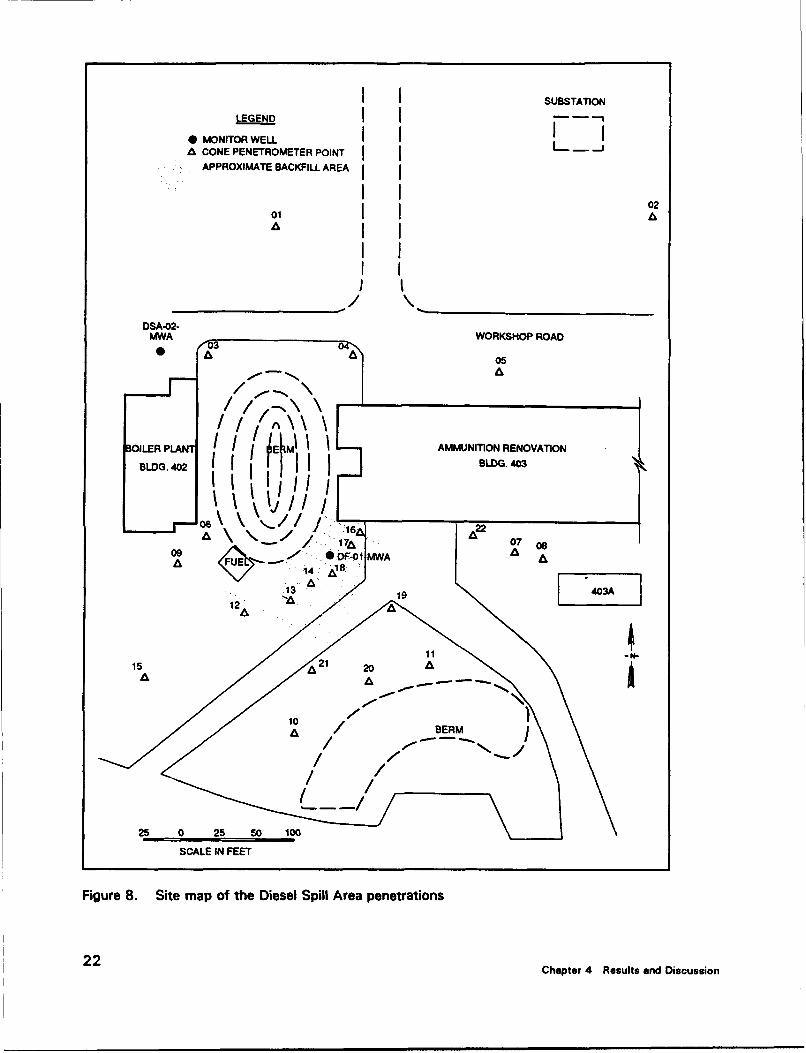
Figure 7 provides an illustration of the pushpipes, probes, and attachmentsutilized at this site, and Figure 8 is a site map of the Diesel Spill Area indicat-ing locations where probe sensor data and physical samples were collected.The approximate area of the investigation covered 5 acres. Each numberedpoint represents a penetration, and each point is designated in Table 1. Thelabels CP-01 through CP-22 indicate sensor data pushpoint locations. Thelabels prefixed "SCP" indicate locations where the soil samples for the WESanalyses were taken. The labels prefixed "DSA" indicate locations where thesamples for the Montgomery Watson, Inc. analyses were taken. The sequenceof operations at this site began with conducting the sensor probe penetrationsfirst (to obtain soil classification and soil fluorescence data), and then conduct-ing physical sampling.
Soil Classification Measurements
Penetration resistance
The first penetrations were conducted on the north side of Building 403.The first penetration was located near CP-04 off the road shoulder, and theprobe was connected to the large diameter (1.75-in.) pushpipe. After pushingto a depth of approximately 13 ft below ground surface (bgs), the reactionforce on the hydraulic rams was not high enough to overcome the soil resis-tance. Seve,:l tu-ther attempts were conducted at adjacent locations, anddeeper penetral,-ns with the 1.75-in. diam pushpipe were not successful. Thesoil classification displayed at the point of refusal typically was betweenSCN 3 and 4, indicating the presence of sand layers.
To determine if deeper penetration could be achieved, two methods wereutilized: prepushing with a "dummy" tip, and field-modifying the pushpipe.Prepushing consisted of pushing a 1.4-in. or 1.75-in. diam empty pushpipestring (no sensor probe attached) to a refusal depth, either once or twice in the
20 Chapter 4 Results and Discussion

PUSHPIPE
1.75" $ 1.4" 4
mi 1
SNOTCHED ROD
FRICTION BREAKER(1*/rPROJECTION)
I SAMPLERS
(DUMMY TIP)
SENSOR PROBE UGOUDAT
FBER OPTIC WINDOW MOSTAP TM
FRICTION SLEEVE
CONE TP
GROUT7nP
NOTE: NOT TO SCALE (FOR ILLUSTRATION ONLY) HPITM HP IITM
Figure 7. Pushpipe configurations
same hole. Field-modifying the pushpipe consisted of welding "friction break-ers" around the pipe circumference, approximately 1 ft above the tip. Thefriction breaker pushpipe was used in both a "dummy" configuration and withthe sensor probe attached. Figure 7 indicated the relative sizes of the push-pipes and attachments utilized during this site investigation. The 1.4-in. diamnotched pushpipe with attached sensor probe was the configuration used for allsensor data collection pushes (CP-O1 through CP-22). All samples were takenusing the 1.4-in. diam notched and unnotched pushpipe configurations.
Chapter 4 Results end Discussion 21
SUBSTATION
LEGENDI IF0 MONITOR WELL,,_1IA CONE PENETROMETER POINT .
APPROXIMATE BACKFILL AREA
0201 A
DSA-2-MWA WORKSHOP ROAD
Q • 05
IjI
_ _ _ _ _ _/,/__\___
(IIE M I AMMUNmO RENOVATION
Oro 1 6-09 17,A 07
0. 0.DOF--01 MWA A AA144 s..
13• "% / 19 403A
152
A0 Il
25 0 25 50 100
SCALE IN FEET
Figure 8. Site map of the Diesel Spill Area penetrations
22Chapter 4 Results and Discussion

Table 1Penetration Points
The points Neted below ae referenced to the Figure 8 site map:
Point Penetration number and adjacent sample points
01 CP-01,1 SCP-0 1
02 CP-O2, SCP-02
03 CP-03
04 CP-04
05 CP-05, SCP-05
06 CP-06. SCP-06
07 CP-07
08 CP-08, SCP-08
09 CP-09. SCP-09
10 CP-10
11 CP-11
12 CP-12, SCP-12
13 CP-13, DSA-04-SC
14 CP-14. SCP-14, DSA-03-SC
15 CP-15, SCP-15
16 CP-16, DSA-01-SC, HP-1
17 CP-17, SCP-17, DSA-02-SC
18 CP-1S
19 CP-19, SCP-19, DSA-05-SC
20 CP-20, SCP-20
21 CP-21
22 CP-22
Legend:CP - Cone penetrometer point.SCP = Soil sample (WES).DSA = Soil sample (MW).HP = Water sample.
Several attempts to achieve deeper penetration with the 1.75-in. diampushpipe were attempted using different combinations of the above two meth-ods. The maximum depth achieved with the 1.75-in. diam pushpipe withsensor probe attached (for data collection) was approximately 30 ft bgs. The1.4-in. pushpipe configuration was used for the remainder of the site investi-gation, and depths to 71 ft bgs were successfully achieved.
Chapter 4 Results and Discussion 23

Several items were observed during the attempt to achieve deeperpenetrations:
a. The friction breaker arrangement achieved an approximately 100 per-cent increase in depth. Pushpipe vibration and "chatter" during penetra-tion was significantly reduced when using the friction breaker.
b. Pushing the sensor probe down a prepushed hole required the prepushedhole to be less than the diameter of the sensor probe if fluorometersensor data were to be collected (assuming the prepushed hole remainedopen, and the soil or contaminant characteristics were notcompromised).
c. Achieving true vertical alignment of the pushpipe as it penetrated thesoil surface was critical for subsequent alignment as the pushpipe pene-trated further into the subsurface. Small objects such as irregularlyshaped surface gravels easily deflected the pushpipe tip from true verti-cal alignment immediately prior to penetration.
d. The soil resistance to penetration was a result of accumulated "skin fric-tion" (shear stresses around the pushpipe shaft circumference) and pointresistance. The observed pushpipe behavior when pushed into pre-pushed holes led to the assumption that skin friction played a majorrole; the cone tip and friction sleeve sensor outputs were in the normal(or below normal) ranges, while the hydraulic ram force gage indicatedexcessive resistance (typically 35,000 lb at the point of "refusal"). Ingeneral, the larger the diameter of pushpipe and attachments (probesand samplers), the shallower the achieved penetration depth. The cir-cumferential area of the 1.75-in. pushpipe was 0.458 fO2/ft of length, the1.4-in. pushpipe was 0.364 ft2/ft of length, and the surface area differ-ence between the two pipe sizes was approximately 20 percent.Assumptions that the 1.4-in. diam pushpipe would achieve approxi-mately 20 percent greater depth than the 1.75-in. pushpipe for a givenram force were observed not to be valid. The smaller pushpipeachieved approximately 100 percent deeper penetration prior to"refusal," based on several comparison observations.
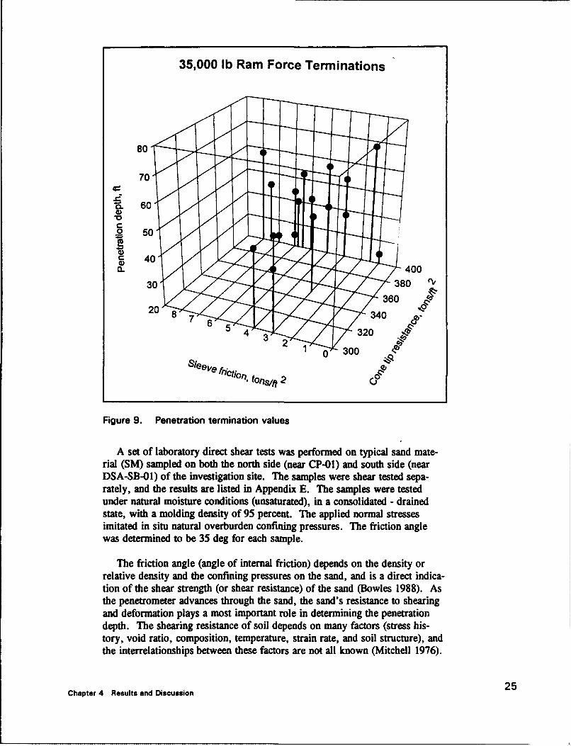
The small diameter (1.4-in.) pushpipe configuration was utilized for theremainder of the sensor probe pushes. The deepest penetration achieved was68-ft bgs (CP-10). The typical penetration depth was approximately 40 to50-ft bgs, and the shallowest was 23-ft bgs (CP-02). All probes were pushedto "refusal." At that point, the hydraulic ram force gage registered 35,000 lb,the cone tip resistance reading ranged from 300 to 400 tons/ft2 (600,000-800,000 lb/ft), and the friction sleeve resistance reading ranged from 3 to8 tons/ft2 (6,000-16,000 lb/ft2). The cone tip reading was typically 400 tons/ft2 at the refusal force of 35,000 lb, indicating that cone tip resistance played amajor role in penetration depth ability. Figure 9 indicates the termination("refusal") values for the penetrations using the 1.4-in. diam pushpipe withattached sensor probe. The soil type at the termination point was typicallysand (SCN 3 to SCN 4).
24 Chapter 4 Results end Discussion
35,000 Ib Ram Force Terminations
80
70
C 6
0 50
400L 400
3 0 " I /•1 • • /"/ 3 8 0360 o
6 5 302
Sleeve fr. 2 00 300"Se v "ctioll, tofns/f 2o
Figure 9. Penetration termination values
A set of laboratory direct shear tests was performed on typical sand mate-rial (SM) sampled on both the north side (near CP-01) and south side (nearDSA-SB-01) of the investigation site. The samples were shear tested sepa-rately, and the results are listed in Appendix E. The samples were testedunder natural moisture conditions (unsaturated), in a consolidated - drainedstate, with a molding density of 95 percent. The applied normal stressesimitated in situ natural overburden confining pressures. The friction anglewas determined to be 35 deg for each sample.
The friction angle (angle of internal friction) depends on the density orrelative density and the confining pressures on the sand, and is a direct indica-tion of the shear strength (or shear resistance) of the sand (Bowles 1988). Asthe penetrometer advances through the sand, the sand's resistance to shearingand deformation plays a most important role in determining the penetrationdepth. The shearing resistance of soil depends on many factors (stress his-tory, void ratio, composition, temperature, strain rate, and soil structure), andthe interrelationships between these factors are not all known (Mitchell 1976).
Chapter 4 Results and Discussion 25

A peak friction angle of 35 deg indicates an approximate relative density of60 percent for a uniform fine sand (U.S. Dept. of Transportation 1978).Neither one of these values is relatively large, and by themselves would notexplain the high resistance to penetration encountered at this site. All of thesamples were "disturbed," i.e. were not in the in situ state of stress at the timeof analysis.
The resistance to penetration was observed to be a function of the accumu-lated "skin friction" during several penetrations into prepushed holes (as previ-ously detailed) and also a function of achieving maximum cone tip resistance(400 tons/ft") at the termination point in the remainder of the penetrations.Based on the limited number of laboratory tests for physical and mechanicalproperties of the soils, it is probable that the high resistance to penetration wasdue to in situ properties not observed in the laboratory samples. Sand cemen-tation or other structural variations may also be responsible for the penetrationresistance behavior. Preliminary studies have indicated that even a smalldegree of sand cementation increases the tip and friction resistance during apenetration event (Puppala, Acar, and Senneset 1993).
Soil classification
The data plots showing the soil classification and soil fluorescence sensorresponses for penetrations CP-01 through CP-22 are included in Appendix D.Except for the northernmost penetrations (CP-01 and CP-02), the surfaceelevation variation for the remainder of the penetrations was within 3 ft.CP-01 and 02 surface elevations were approximately 4 ft lower than theremainder of penetrations. The deepest depth achieved was 68 ft bgs (CP-10),and the shallowest depth was 23 ft bgs (CP-02).
The predominant stratigraphy consisted of coarser-grained deposits (sands)with interbedded finer-grained deposits (silts and clays). A very general trendwas the presence of sands above the depths of 19-22 ft bgs, a 1-4 ft layer offiner-grained material, then a 10-ft layer of sand underlain by another finer-grained layer.
Penetrations CP-01 and CP-02 indicated a finer-grained layer locatedapproximately 4-ft bgs. A hand auger was used adjacent to those penetrationsfor the purpose of visual soil classification to depths of approximately 15 ft.The type of soil encountered (below the loose sand/gravel surface) was pre-dominately uniform fine sand, brown in color, and with varying (visual) mois-ture contents. A finer-grained (white silty material with very small rockfragments) layer was observed at approximately 4 ft bgs, and was approxi-mately 2 ft thick. The soil type visual classification matched the penetrometersensor classification to a depth of 15 ft. Penetrations CP-04 and CP-05 indi-cated the presence of this silty layer at the same elevations as seen in CP-01and CP-02.
The CP-03 data log indicated a clay layer at 9 ft bgs overlain by fine-grained material. The clay "spike" at 9 ft was in reality an abandoned 12-in.
26 Chapter 4 Results and Discussion
diam steam line (traced back into Building 402), and was overlain by backfillmaterial. The old metal pipe was penetrated without damage to the penetrom-eter probe.
Both CP-03 and CP-04 logs indicated a clay layer between 30 and35 ft bgs. CP-05 was the deepest penetration on the north side of Build-ing 403 (to a depth of 50 ft), and indicated another (lower) clay layer at46 ft bgs. No data were collected in the first 5 ft of CP-05 due to the neces-sity of using a "dummy" probe to penetrate the asphalt pavement and subbasematerials.
The remainder of penetrations (CP-06 through CP-22) surrounded theoriginal diesel spill site. Parts of the site had been previously excavated andbackfilled with "clean" materials up to depths of 30 ft. The exact extent ofthe excavation and the contractual specifications for the backfill operationwere for the most part unknown, based on conversations with site personnel.The approximate extent is indicated in Figure 8.
The backfill limits were presumed from the penetrometer data, based on thepresence of three "fingerprints": the cone tip response, the friction sleeveresponse, and their combined response indicating a fairly prominent clay layerat approximately 20 ft bgs. The presence of backfill materials was presumedwhen the cone tip and friction sleeve response exhibited a curved pattern oflow stress that increased sharply with depth. This type of response is exhib-ited if granular materials are loose or if cohesive materials are underconsoli-dated (U.S. Dept. of Transportation 1978). The connection between backfilllimits and low stress response from the sensors is tenuous if the backfill mate-rial was densely compacted. The presence of the clay layer at approximately20 ft deep appears to be the uppermost confining layer (possible aquitard) andis composed of a 1- to 2-ft thick clay layer. The presence of this clay layer inall penetration logs noted (with the possible exceptions of CP-13 and CP-21)indicated that it most likely was a natural, not backfilled, layer.
A silty layer with imbedded small rock fragments approximately 1- to 2-ftthick was observed at depths ranging from 5 to 10 ft bgs at penetrationsCP-10, 15, 21, and 22. This layer appeared similar to the silty materialobserved at penetrations CP-01, 02, 04, and 05 on the north side of Build-ing 403. A sample retrieved from this layer at CP-15 served to verify thepenetrometer sensor soil classification and also correlated with the hand-augered samples taken at CP-01 and 02. It was assumed that this layer wasanother indicator of the undisturbed soil surrounding the backfilled area. Dueto the presence of fluorescence observed in this soil layer (discussed in a latersection of this report), the particles in this material were analyzed by stereo-scopic microscope and X-ray diffraction examinations. The conglomeraticparticles consisted of rounded fragments of sand and pebbles, cemented with aclay-sized calcite material. After chemically removing the calcite (calciumcarbonate), the remaining minerals were observed to be quartz, potassiumfeldspar, plagioclase feldspar, and monoclinic amphibile. Quartz and feldsparwere the major minerals present. Figure 10 shows a representative X-raydiffraction pattern of this material.
27Chapter 4 Results and Discussion

0
(00
CU
0
CU
C) 4
00';
310
CuD
* C;
Chpe 4 eulsad icuso
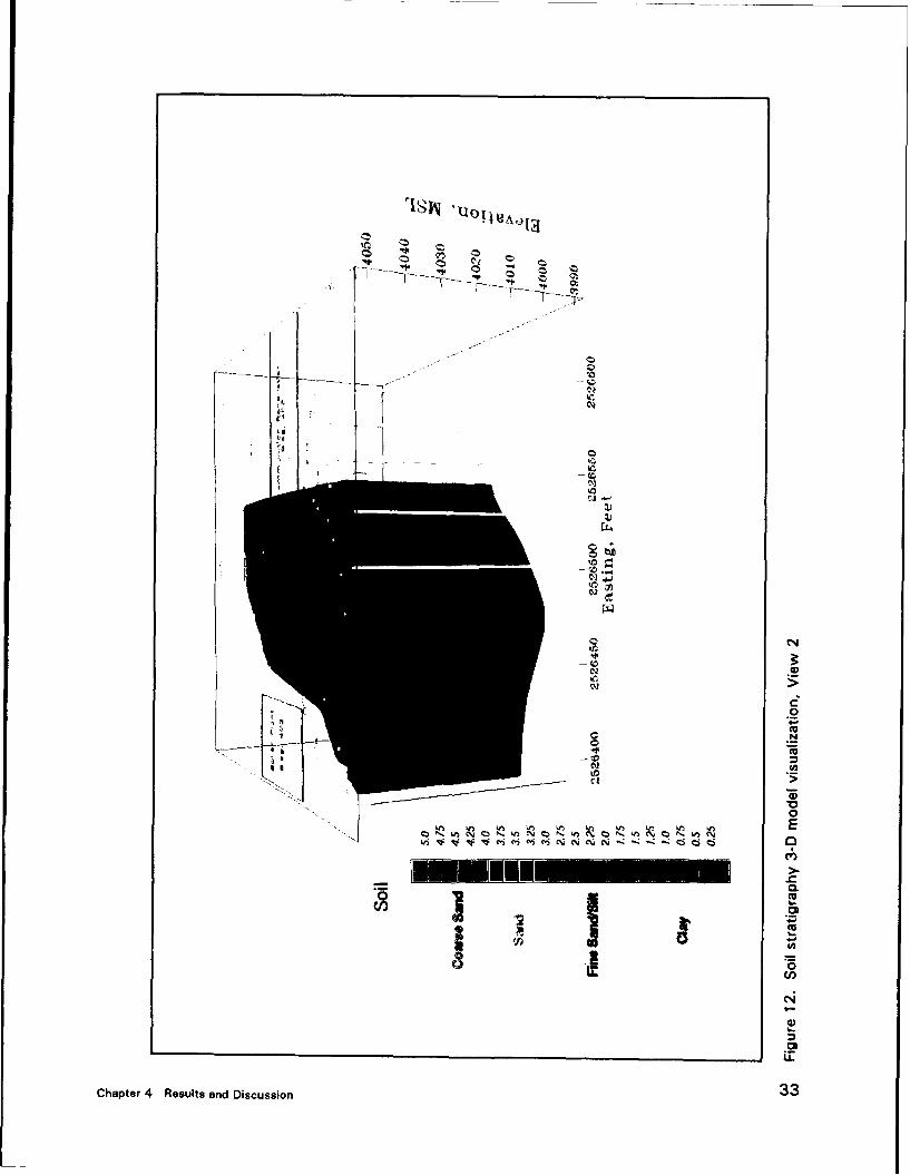
Figures 11 and 12 show the postprocessed soil stratigraphy data presentedas a three-dimensional model visualization. The general trends correlate fairlywell with the stratigraphy indicated by the individual push plots.
The retrieved soil samples were laboratory-analyzed for soil classificationinformation. The gradation curves and soil classification information forrepresentative soil samples are shown in Appendix E. Note that the predomi-nate soil type was pc,)rly graded sand (SM to SP). The silt layer containingcalcite fragments was a sandy silt (ML). The dominant sand particle shapewas subangular.
Soil Fluorescence
Soil fluorescence background level was typically less than 100 countsintensity. Fluorescence greater than that level was observed at various depthsduring all penetrations CP-01 through CP-22. The data plots for each pene-tration are shown in the Appendix D.
Fluorescence peaks up to approximately 550 counts (intensity) wereobserved in some of the penetrations on the north side of the Building 403diesel spill site. The maximum intensity occurred in the silt layer previouslydiscussed in the Soil Classification section above. This layer occurred atdepths between 3 to 9 ft bgs. Samples taken from the silt layer were analyzedas discussed in the Soil Classification section above. These retrieved sampleswere also analyzed by the fluorometer, and fluorescence matching the in situresponse was observed. The X-ray diffraction pattern (shown in Figure 10)indicated that the conglomeratic pebble fragments were coated with the min-eral calcite. Calcite is a known ultraviolet fluorescent mineral (Dana 1959).
The remainder of penetrations (closer to the diesel spill area) indicatedfluorescence levels above background at depths typically between 5 to20 ft bgs. Maximum fluorescence intensity in the area closest to the spill sitewas approximately 700 counts at peak wavelengths around 450 nanometers.Fluorescence responses were not observed at deeper depths with the exceptionof CP-16 and CP-17. These two locations are immediately adjacent to thepresumed original source of the diesel spill (south of the Bldg. 403 mechanicalroom). Fluorescence patterns were observed in an approximate interval of12- to 45-ft bgs at these penetration locations. CP-17 penetrated to within 3 ftabove the presumed water table elevation (62 ft), and no fluorescence wasnoted at that depth. The only other penetration which went to the water tabledepth was CP-10 (approximately 150 ft southwest of CP-17); no fluorescencewas observed in the water table zone.
Figures 13 and 14 are the postprocessed fluorometer data presented asthree-dimensional model visualizations. The total fluorescence was gridded asa function of spatial distribution, and the visualizations represent all fluores-cence sources observed. No distinction is made between contaminationfluorescence and other source fluorescence.
29Chapter 4 Results and Discussion
Figures 15 through 22 are the three-dimensional visualizations with theinterference fluorescence patterns subtracted (filtered out). The interferencepatterns were identified from onsite POL verification sampling and analysis(discussed in detail in a later section of this report). The visualizations indi-cated in Figures 15 through 22 represent probable POL contamination at thesite based on the results of the verification soil sample analyses. Four orienta-tions are presented; view "a" represents intensities above 100 normalizedcounts, and view "b" represents intensities above 200 normalized counts.Note the difference between Figures 13 and 14 (total fluorescence) and Fig-ures 15 through 22 (filtered fluorescence).
Support Systems
Data collected from some of the support syste:ns (site surveying and sam-pling) were for the purpose of complementing the primary data collectionefforts using the probe sensors. The remainder of support systems data col-lection efforts was mostly observational (geophysics, probe decontamination,and grouting) and served specific functions.
Surveying and geophysics
The site surveying data were obtained by establishing a central point fromwhich sideshots were taken. Known x and y coordinates (California StatePlane Zone 1) and ground elevations (referenced to mean sea level) of moni-toring wells DF-01-MWA and DSA-02-MWA provided reference points for atwo-point resection which located a central surveying point on top of the bermbetween Buildings 402 and 403. Multiple sideshots were taken to determinethe coordinates and elevations of penetration points. A traverse was not per-formed to determine the data precision and accuracy, but repeated sideshotsobtained over the project duration served to validate the data quality. Accu-racy of surveying data was expected to be within plus or minus 2 in. Thedata (coordinates and elevation) are shown in Appendix B.
A very limited geophysics program for locating underground obstacles wasperformed. The SIAD assistance efforts in locating utility and fuel lines in thevicinity of proposed penetrations minimized these requirements. An electricalduct bank near CP-05 and possible buried debris near CP-09 constituted theprimary targets for SCAPS geophysics. The area near CP-03 was not a tar-geted area due to prior SIAD clearance from presence of active utility lines.
Grouting
Grouting through the umbilical cord grout tube was performed at the pene-tration locations. The grout formulation used (a portland cement material withbentonite added) was a successful first-time achievement at a SCAPS site.The penetrations for sampling soil or grounc :iter were manually grouted (due
30 Chapter 4 Results and Discussion

., .,
.0
0.
tfi v w 4,mc;Ci NC z
0
I ,a
.2LL
ni i on
Chpe 4Rslt.- Dsusin3
' 1 8N
00
S -- ......
-•L
c• .,4-.
Chapter~~~~_ 4 eut adDsusin3
I._.
-..4-
0 -. 7:. _ _ . - C.
N
a,i
Chaper ResltsandDiscssin 0
- -.. ------- 4
--
C)C
cc
• U
Co
o)
Q 4)
0
0(n
6
LL
.C5
Chaper ResltsandDiscssin 3

I -
I'. - --- -
-I
CV
0,0
NN
0
(Z)
to
"0 Plol ,-,M 0
0
._4-N
(n
37Chapter 4 Results and Discussion
J0
---- Mo
eii0
(U0
0
4-
0
z>
cp)0.0
00
0
C0
(D
4-
39Chaper 4 Reslts nd iscusio
70
C•
0
z
CDO
C•,
0
-----------
S........0y
S... ---- ... . -- ....----- >
u• 0 % ,,
0
-- ---- 0 0
N
._
0
0
U,
41Chapter 4 Results and Discussion
I"%0
CO
1C1
"."u~ ..... NJJE•..f-l'
Chate 4, Reslt and Disusio
00
00
cc°
o40hpe 4 euls.d icuso

,13
CO
to
4.d
-:4
0!.J0"0
"•. (N
0
i.206
U-
45
Chapter 4 Results and Discussion

00
ci
0
ci
C'.?
0
-Ca -.4-.
ci
0
4-- Ca
C'?
C'?
(Ucv)a
o4
ci
C?C0
(UN
.L � aw
-' �
0
'tI (1 Cv)
i5� V0000 C
o0000�� V0(aV
0
.4--4
C,,
0)
VI..
.Iz
47Chapter 4 Results and Discussion
IL.I
C',"
Le4-
_________________CD__CID______ Q__Q_ Q C'
CC
o .0
00
CN
LL
Chaper ResltsandDiscssin 4

-,
44
Lu
>
d.2N
=ram,,
3-O
0
LM
____________ '
'4-J
(I,
L-
c'J
51Chapter 4 Results and Discussion
LMN.,•
/
Lfj .)
Cý
04
.9L.NCEhaUter 4Rs
.C_
0
e|
0
cir
53Chapter 4 Results and Discussion

to the lack of an umbilical cord) with a thicker consistency of grout. Thegrout mixture with bentonite added (3:2 cement to water ratio by weight, plus2 percent bentonite) tended to slowly clog the pump output line, especially atthe connection points where turbulent flow occurred. The grout tended to"settle out" at those points, probably due to minute changes in velocity, andfrequent cleaning and tube clearing had to be accomplished.
Tube clearing (a standard procedure to prevent clogging) was done bypumping fresh water through to gradually dilute the slurry. The tube wasconsidered clean when clear water was seen shooting out the probe tip (as theprobe was hanging underneath the truck).
Soil and groundwater sampling
Sampling operati ns encountered the same problem as the sensor penetra-tions, namely that the soil resistance prevented most of the samplers fromreaching targeted depths. The small diameter (1.4-in.) pushpipe was used topush the soil and groundwater samplers previously listed.
The Gouda7 sampler was pushed to the target depths (approximately61-ft bgs into the "smear zone" above the water table) for retrieving the sam-pies for Montgomery Watson, Inc. analyses, but its small size prevented largesamples from being retrieved. The Mostap' sampler would have retrieved anideal larger sample size, but its larger diameter (2 in. versus the Gouda's1.75 in.) could not overcome the soil resistance for penetration to 61-ft bgs.Once the sample was retrieved, extricating it from the sampler tube wastedious and time consuming.
The Mostapr sampler was pushed to the target depths (approximately 4- to20-ft bgs) for the sample verification project discussed in other sections of thisreport. Since the sample tube was a split tube arrangement, extricating thesample was not difficult. Some mechanical elements within the sampler weremore delicate than those in the Gouda7 sampler, however.
The Hydropunch" Models I and II were used for obtaining groundwatersamples. Only the smaller Model I (1.75 in. outside diameter) achieved thetarget sampling depth (below the water table), and only one sample wasretrieved. The maximum sample size using the Model I is about 500 mt,which falls short of the standard testing laboratory requirement of 1 f mini-mum. After several attempts which took approximately one working day, itwas decided that further attempts to collect groundwater samples in this siteenvironment would be futile. Groundwater samples could have been obtainedfrom the upper portion of the unconfined aquifer, but the efforts to retrievethem would have not been cost effective.
The practice of "prepushing" a hole prior to penetration with a samplerwas attempted and was not as practical as doing so with the sensor probe.Both soil samplers would automatically engage into the open position whenlowered into a prepushed hole. The groundwater samplers had more
55Chapter 4 Results and Discussion

resistance to such engagement, but on occasion they would engage prior toreaching the termination depth of the prepushed hole. Even when the pre-pushed hole penetrated well below the water table elevation, the groundwatersampler, in most cases, either did not reach that depth or prematurelyengaged.
Cleaning and decontaminating each soil and groundwater sampler wasrequired after its use. The steam cleaner (hot pressure washer) was utilizedfor cleaning, and distilled water rinsedown provided decontamination. Ingeneral, the groundwater samplers were more delicate than the soil samplers.They contained more intricate mechanisms which provided greater mainte-nance and cleaning challenges.
Penetrometer Fluorescence Verification
Laboratory calibration studies
The results of analysis of the laboratory fortified soil samples (Native andFill) obtained from SIAD prior to the SCAPS deployment are summarized inTable 2. This table only contains a TPAH value which is the sum of allpolynuclear aromatic hydrocarbons (PAH's) detected for a particular sample.The levels of the individual PAH's in the soil samples are presented inTable 3. The triplicate analyses of each fortification level indicate that thesamples contain homogeneously distributed POL contamination. These datasupport the efficacy of the WES soil POL fortification procedure for construc-tion of samples with diesel fuel.
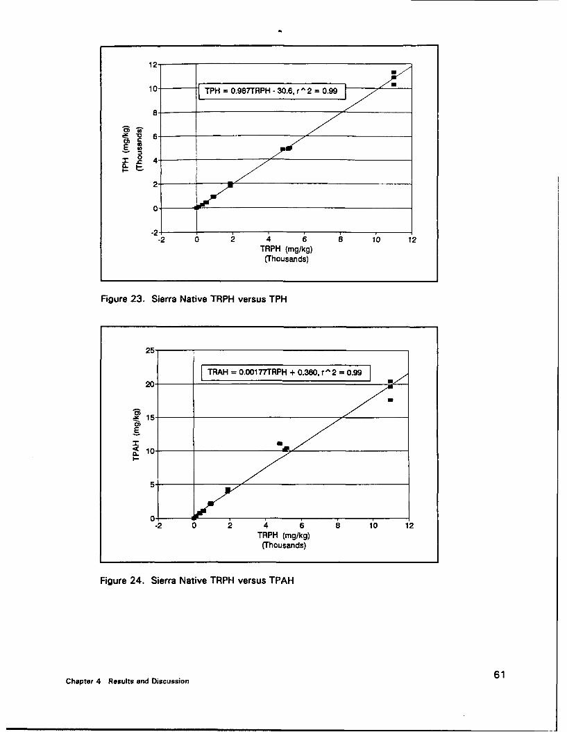
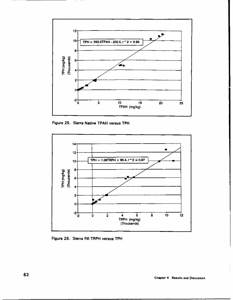
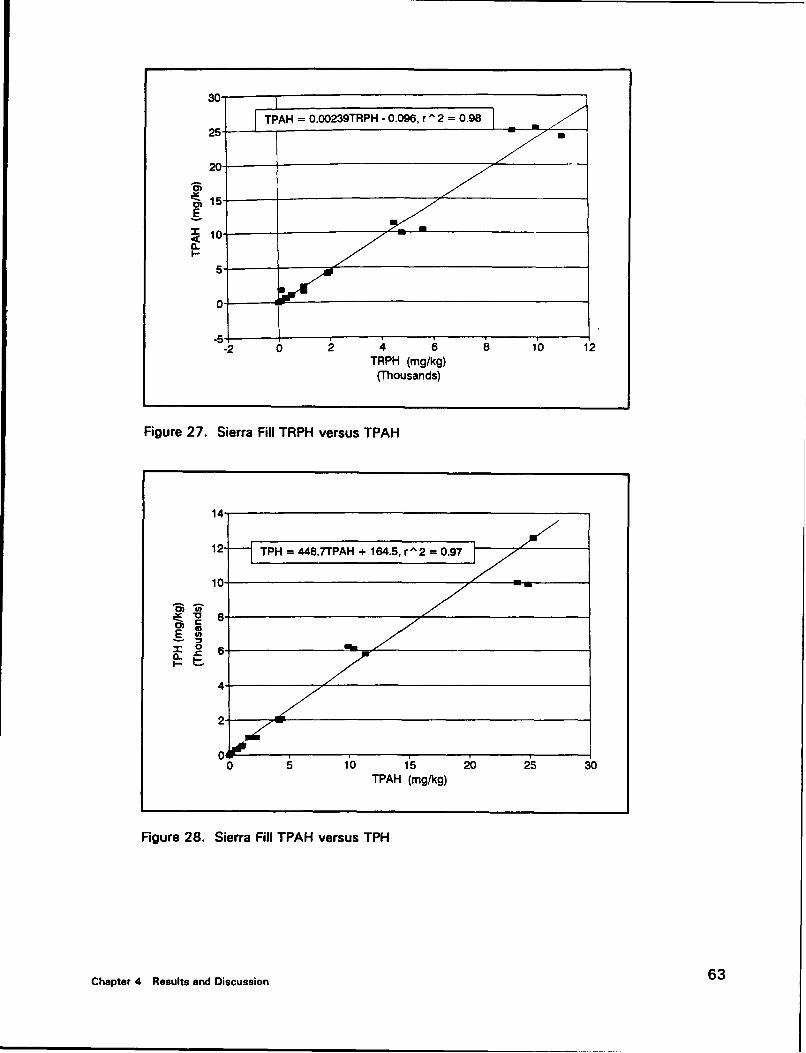
The data indicate strong linear relationships between the different parame-ters (TRPH, TPH and TPAH) investigated as measures of POL contamination.The Native soil sample exhibited strong linear correlations between TRPH andTPH (r2 = 0.99, Figure 23); TRPH and TPAH (r' = 0.99, Figure 24) andTPAH and TPH (r' = 0.99, Figure 25). The Fill sample also exhibitedstrong linear correlations between these parameters: TRPH and TPH(r' = 0.97, Figure 26); TRPH and TPAH (r' = 0.98, Figure 27) and TPAHand TPH (r' = 0.97, Figure 28). The strong linear correlations betweenthese different measures of POL contamination indicate that, for this set offortified soil samples, these different measures of POL contamination are allcomparable to one another. This result is not surprising since all the soilsamples were fortified with aliquots of the same diesel fuel. Lower correla-tion coefficients between these measures of POL contamination would beexpected for soils that contain mixtures of different POL types or a singlePOCL type that has been allowed to age in the soil. The TPH procedure (EPAMethod 8015) includes calibration with a particular fuel (EPA 1984), thus amixture of POL types or an aged single fuel would cause biased results in thismethod.
56 Chapter 4 Results and Discussion
- - - --- - ý *R =r -
*E E
(' (' (' C4 U) M) 0 44 N 0ris~ 0- LO It. It -. 0 o
E -
a 0 0 a0 (' 0' 0 i. 01
LL a 0 0 4 4 (' (4 4 0 0E
ILt ma l n L
COC
_00 0 0 0 0 0 -
z U) U ) U ) U ) ('4 (n U) U) ) -E
C 2 E
CL 8
* 0 00 80 0 0 0 a
2L 0 a
2 M 0 *
(0 *
E
:~~n0 0 0 0 0 0 0 0 0 - 0 .2.
S.E. a-
o 0 00 0 0 0 a) 4 0 0 C
z 0) U 0 0 P U) a) U) 0 a )
Chapter~~~(' 4 Reut an4icuso
- m - - 2 mý -ý - M V) - M -
W2 C - -
~* a) - 4' 0 0 ( ) . 4
am C4 (4' ' - 0o 0 ' ) a'
'E Cq t4 C4
w 0 8 0 0 000 0"0) wo a) C 0 cc
'm 8 o 00 8 8 8 8
E C
z 0 t0 l an (4 n 4' 4' w 0 0 0
0U 0
0!
P E- - - C4
00--0 00N 06 o M w 0 0
Co 2 228 8E)-
S 2 2 Z 2 2 2
I-co 0 A (A (A 8A 8A ( A ( A 0 A (----------------------------------- -------------------------------
58 6 0 ' 00
58 Chapter 4 Results and Discussion
Is o 0 080 0 0 0 0 0 0 0 0 0 0
6 6 o oo 0 a 0a 0 o 66 a
~ 88 88 88 8 8 8 8 .88 8. 8. 8. 8 8 8 8 t
Z21
22
WI& -C
Ez
CL
~ a. o o o o o o d d o d d o lo o ld ,.~ W, C
U N*O W <l~ 0.2
8 88 800 8N si 1
E 0 0 0 rw0 . ~
z 8m 86 ~ ~ 6- 0 -1 1 11 1 lo
CO
8 8 8 * 8
0C o Z Z 2 Z Z Z 22 z z 2 z z o oo000000 1
- z ' 6 ' * U 6 h
Chaper 4Resuts ad Dicusson 5

m - -0 ; -6 U U U U 0 -- -I d 1 d , H ;-
8. 8.8 .8 8. 8.s S.l l .l 8 8 8i. 8. . 8. 8 8S 8 8 80 o o 0 a 0 o0~~ o 0I o o a6 0 0 6 0CO 0 0 *1 1o
0 01 0000 00a0 0 00 00 00 00
Ss 8.8.8.88s 8. 8.. 8.~lI. 8...88 s .. 8.•.. .80 . 8 R.8R 8 $. 8. R .8 8. 8 R $ .R .88 .R
ro o 0 o o 01 0 o0~~ 0 0~ o 0 0111 a 0 o 0 o COo
8i 8
So a o o 011 0 0l10l CO 010 0 0 0 01 o 0
0 0 0"1 01016 oP ! 0 OR o a o; o 0 0100
1 0 60 0 001 000 010000 0 100 10 0616101o 1
Ft 8 8 8.88888. 8.8 .8s
00 a0 0 0 0 0 0 a0 0 0 0 0 0 010
ms ss Ss S4 •14.1.1 :2 Is 0 "0•r••
8r 8 8 s88888.5.88...88.8..5
I 6 6 o o o~l~O o o o o o o o o o 6
6 00 106 6 o o o o d d d o o Old d
En 0 0 0:, 1 . .0l
12 1.0 0 0 8 8 8J0~i
60 Chapter 4 Results and Discussion
12o
10TPH = 0.987TRPH- 30.6, r 2 = 0.99
8
-2 0 2 4 6 8 10 12TRPH (mg/kg)
(Thousands)
Figure 23. Sierra Native TRPH versus TPH
251
20
"~ 15
< 10
4--
0-
-2 0 2 4 6 8 1,0 1'2
TRPH (mg/kg)(Thousands)
Figure 24. Sierra Native TRPH versus TPAH
561
C h a te 4R A R esult 7 7 T R P D isc ussio n0 .9
t2-
10 TPH =550.9TPAH -202.5, r2 =0.99
8-
02 1,0 i's o2 25TPAH (mg/kg)
Figure 25. Sierra Native TPAH versus TPH
1.2
10. TPH = 1.08TRPH + 96.4, r 2 = 0.97
10-
o~
0
-2.-2 0 2 4 6 8 10 12
TRPH (mg/kg)(Thousands)
Figure 26. Sierra Fill TRPH versus TPH
62 Chapter 4 Results and Discussion
30I
TPAH = 0.00239TRPH - 0.096, r 2 = 0.98 -25 - -
20-
I 10- 'CL
5-
0 E
-2 0 2 4 6 8 10 12TRPH (mg/kg)
(Thousands)
Figure 27. Sierra Fill TRPH versus TPAH
14
4-
12 TPH = 448.TPAH + 164.5, r 2 = 0.9ý7
10-
~8.0)
iso
4
2-
0 1'0 1'5 2'0 2'5 30
TPAH (mg/kg)
Figure 28. Sierra Fill TPAH versus TPH
Chapter 4 Results and Discussion 63

Linear relationships were also obtained for both the Native and Fill forti-fied soil samples when the POL measures were correlated with the LIF datacollected from these samples. The Native soil showed stronger linear correla-tions between the POL measures and LIF than did the Fill soil. The correla-tions between LIF and TRPH (Figure 29), TPH (Figure 30) and TPAH(Figure 31) for the fortified Native soil samples were very strong (r' = 0.99in all cases). The correlations between LIF and the POL measures for the Fillsoil samples were also strong but were weaker than those observed for theNative soil samples (TRPH (Figure 32), r2 = 0.97), TPH (Figure 33,r2 = 0.95)) except for the TPAH (Figure 34, r2 = 0.99). Figures 29through 34 are considered laboratory calibration curves for the SCAPS POLsensor and may be used to predict the POL concentration of soils in the fieldbased on the soil LIF response.
The lower levels of correlation observed for the Fill soil between thefluorescence and the parameters used to measure the POL may be the result ofa matrix effect in this sample compared with the Native soil sample. The Fillsample appeared to have a higher clay content compared with the very sandyNative soil. The lower level of correlation between the POL parameters andthe fluorescence for the Fill sample may be the result of less homogeneousmixing of the Fill soil samples than the Native samples at the micro level. Itshould be noted that the LIF sensor only views a very small sample areaadjacent to the SCAPS sapphire window while the POL measurements ofTRPH, TPH and TPAH all use sample sizes of 20 to 30 g.
Another difference observed between the Native and Fill LIF results is thatthe slope of the regression equation between fluorescence and any of the POLparameters is always lower for the Fill samples than for the Native. This isillustrated by comparing the slopes for the relationship between TRPH andfluorescence in Figures 29 and 32 for the Native (0.0468) and Fill (0.0216),respectively. The units of the slope of this line are fluorescence counts/(mg/kg TRPH). Since the slope of the Native soil is over twice the value ofthe Fill soil, this means that the Native soil yields over twice the fluorescenceper unit POL contamination compared with the Fill soil. The slopes of thelines for the other POL parameters with fluorescence are also over twice ashigh for the Native soil as for the Fill (see Figures 30, 31, 33, and 34). Apitzet al. (1992) has reported significantly reduced fluorescence of POL's as theclay content of the soil matrix increases. Therefore, these results are consis-tent with the Fill soil containing more clay than the Native soil.
Field and laboratory analysis of field soil samples
Soil samples were collected at SIAD by WES to investigate the feasibilityof field calibration and verification of the SCAPS POL sensor LIF response.As discussed earlier, the purpose of this investigation were multipleincluding:
64 Chapter 4 Results and Discussion
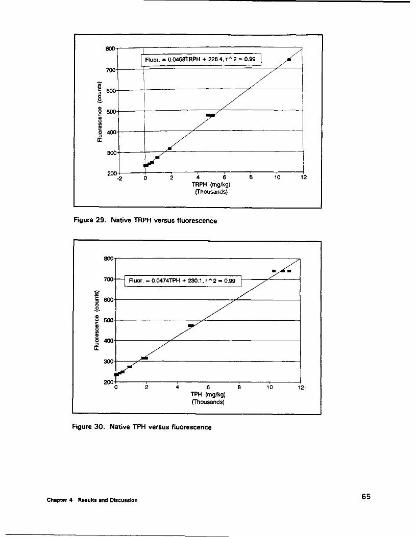
800-
800-- IFluor. = 0.0468TRPH + 228.4, r^ 2 = 0.997971
60700
5600-4)
3O00200
200-
-2 0 2 4 6 8 10 12TRPH (mg/kg)
(Thousands)
Figure 29. Native TRPH versus fluorescence
700--- FRuor. = 0.0474TPH + 230.1, r-2 = 0.99ý
toC600-
0
to
Z5 400-.2
o L 4 0 0 -
300
2O0 2 , 6 1'0 12"
TPH (mg/kg)(Thousands)
Figure 30. Native TPH versus fluorescence
Chapter 4 Results and Discussion 65
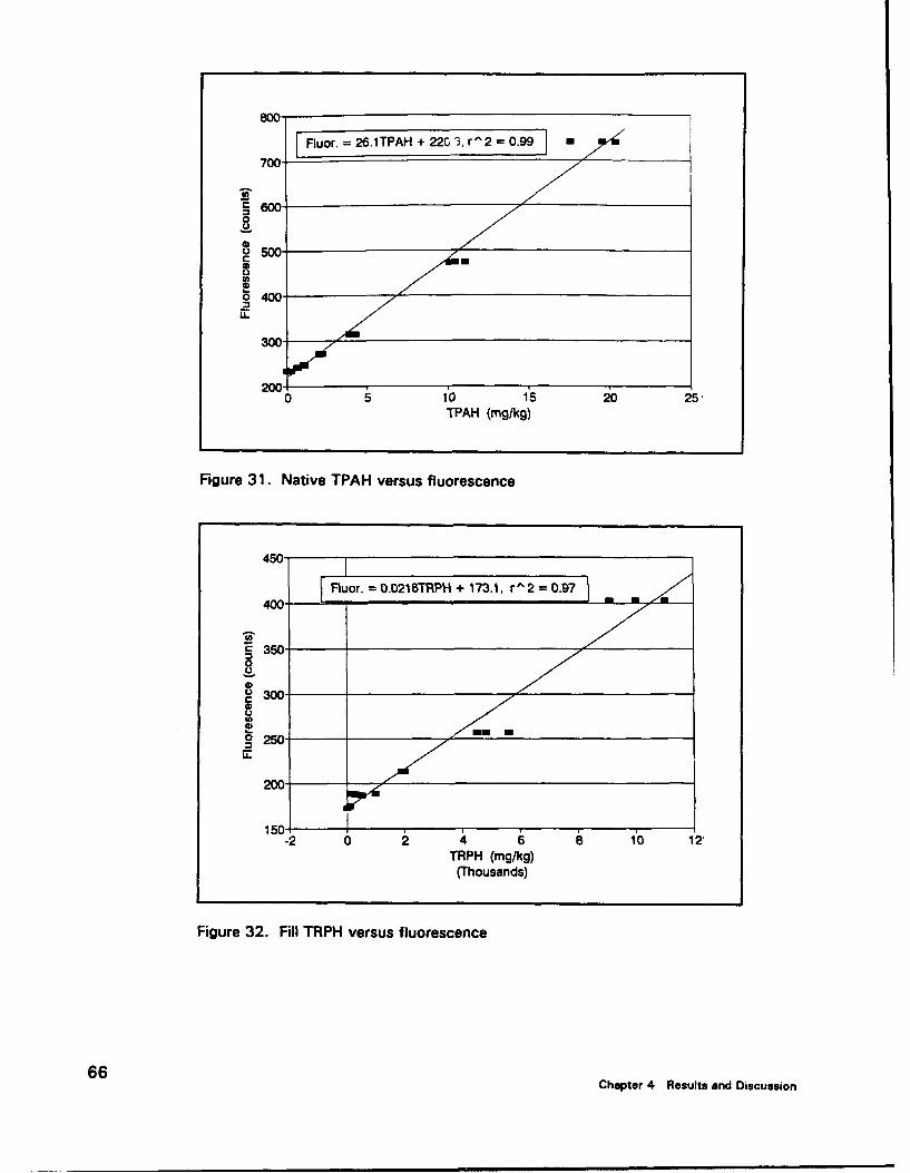
800 [00 Fluor.=26.1 TPAH +22r, 3, r ̂ 2 =0.99 J m
700-
a 00-0
500o
2 o 1 ,0 1' 5 2 2 s 5 ,TPAH (mg/kq)
Figure 3 1. Native TPAH versus fluorescence
450 1
400 Mu r. = 0216TRPHi + 173.1, r ^ 2 =0.97 .
Um
50
300-
ls-2 2 4 1,0 12,TRPH (mg/kg)
(Thousands)
Figure 32. Fill TRPH versus fluorescence
66Chapter 4 Results and Discussion
45--0m l• lmm m m mm m m m m mm m m m m l
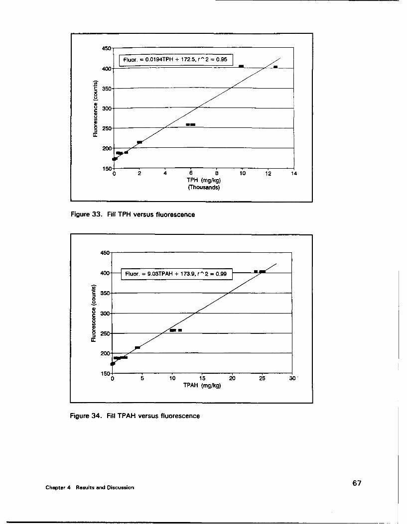
450IFluOr.=0.0194TPH +172.5,r'r2 0.95 I
400-
350
0
.3 0 20 0
TPH (mg/kg)(Thousands)
Figure 33. Fill TPH versus fluorescence
450.
400- Fluor. =9.03TPAH + 173.9, r ^2 =0.99 /
•"350-
0
Cu 300-
U.
SI
o 250-
10o 1,0 1'5 2b 0 s 1 01TPAH (mg/kg)
Figure 34. Fill TPAH versus fluorescence
Chapter 4 Results and Discussion 6

a. Investigation of the utility of a field portable TRPH instrument foronsite verification of POL contamination identified by the SCAPS POLsensor.
b. Collection of soil samples for laboratory analysis to verify POL con-tamination identified by the SCAPS POL sensor.
c. Investigation of the feasibility of onsite POL sensor calibration withactual field contaminated soil samples us..;ig a field portable TRPHinstrument.
Twenty-two samples were obtained from locations at SIAD that had pro-duced LIF response on initial SCAPS POL sensor pushes. The samples werehomogenized in the field, analyzed for TRPH using a field portable fixedwavelength IR detector (Horiba Model OCMA 220), analyzed in the field forLIF response, and analyzed in the laboratory for TRPH, TPH and TPAH.The results of the analysis of these field soil samples are summarized inTable 4. This table only contains a TPAH value for each sample that is thesum of all PAH's detected. The levels of the individual PAH's in the soilsamples are presented in Table 5.
Verification of POL sensor LIF response
All soil samples obtained for field verification yielded detectable fluores-cence when analyzed in the field with the SCAPS POL sensor by pressing thehomogenized soil sample against the probe window. The LIF data presentedin Table 4 and the Appendix D indicate that the field samples were indeedobtained from depths that exhibited fluorescent response. However, compari-son of the LIF response with the TRPH (both field and laboratory determina-tions), TPH and TPAH data obtained from analysis of the field samples leadsto the conclusion that some of the soil samples obtained exhibited significantLIF response in the absence of POL contamination. These samples can beconsidered false positives for POL contamination based on their positive LIFsensor response and lack of detectable POL contamination. The fluorescenceresponse of these samples was suspected in the field of originating from min-erals present in the soil. This was based on their high fluorescence responseand their low TRPH values measured with the !-oriba OCMA 220. Analysisof the fragment particles in those samples confirmed the presence of calcite, amineral kno%.i to fluoresce.
Total recoverable petroleum hydrocarbons
The determination of TRPH on soil samples in the field using the HoribaOMCA 220 allowed the onsite discrimination of fluorescence that was trulythe result of POL contamination from the LIF response due to mineral fluores-cence. The field TRPH measurements indicated that 13 of the 22 samplesobtained were positive for TRPH. The remaining 9 soil samples yielded LIFresponse but appeared to contain no or very low level (< 10 mg/kg) TRPH.
68 Chapter 4 Results and Discussion

- m-- 0 - =- N 4 c
S0 U,1 !- •I
C4
0 !j 0 0 0 0 0 0 0 0 00 0 O 0 0 0 0 0 0
04 It 0 0 Cl -4 C
V 0 Co - f-v v
- 4 C I -i -t . . .
E v Ov, O • c2,N v - v v v v v v v v v v v v V
W n- - WC O -W. U) N
4 e q m 0 Ln It C4 cc 4 .V 4 N N • N • N • IN C4 Od C4 N N• -
4 Pv v v v v v v v v v v v v vCO
~v wI • D • 0 N m • -- In •- -•D CO ,• •I ý' -' M M' •
------------------------------------------------------------------------------------------------
- - - 0 ) , - -- - - - - - - - - - - - -----. 0
0 0) 0 - U) 0 4 U) .O U) r) U -U -*' " U) ) U) U) U) U) 0 0
Cl Cl 0 ) 0 Cl 0 Cl Cl 0 Cl Cl Cl Cl Cl Cl Cl Cl Cl Cl O 0
Ei VM . oo- (-
* ..
0
SOWO C, 'nO U) U U )U "t))U U )*~ 0 0 Cl " -w -. - ------------------ 0 0 m
Chapter 4 Results andVDiscussion
00 -L U!) Cl * -c! 0) L_: -:U 10mz -6 6 6 E4 ;0
aa 0I*-CL2 IL a 2 0 .0 .a
0 U 0 , UU UU UUIU U U U UU UU.
Chpe o eutsadDsuso 69
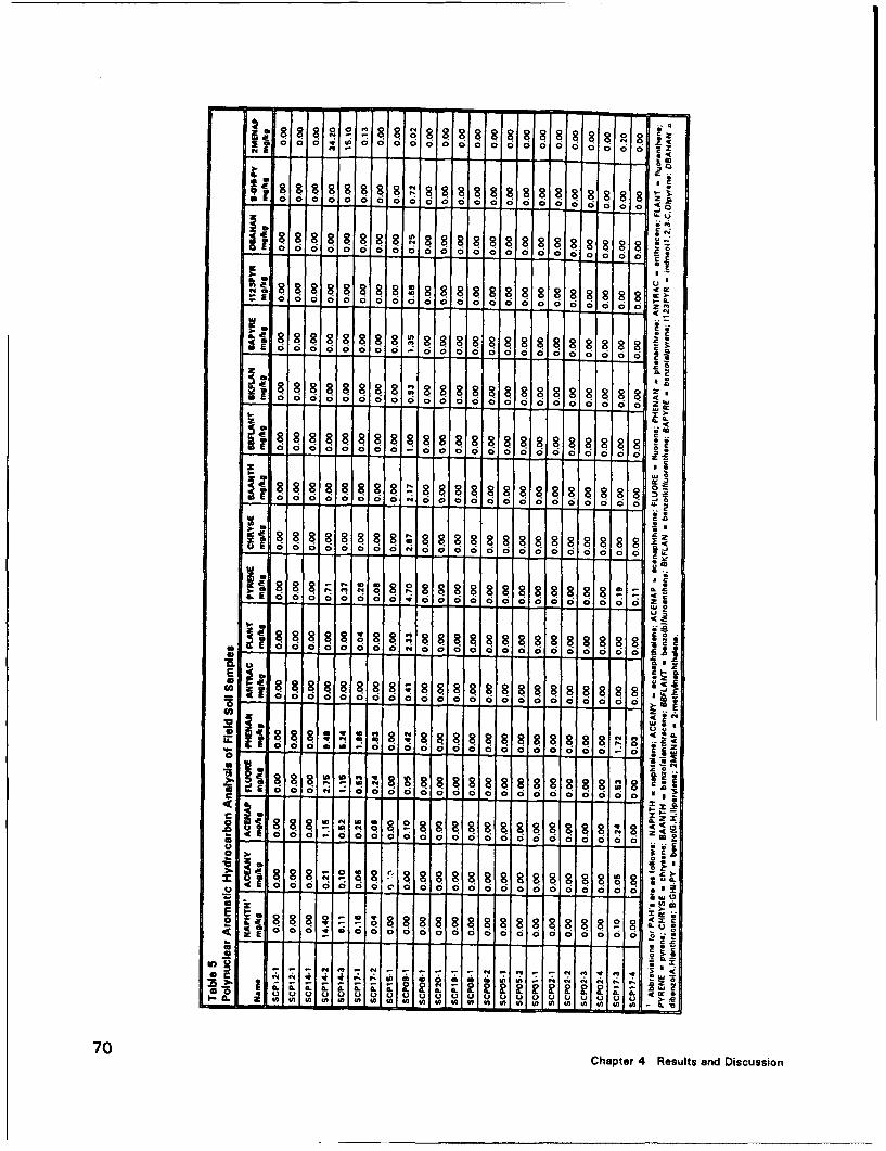
. . . :! 8 8 8 8:8 -. e 8 1 1
0 6
S 8 1'8 8 8 8I s z'
a 0oo 6 0 6 6 01 0 0 000 0010 0 0 0 0z
i .818888,8 $ 88 8 8 8 8 8 8 88888
~~~ o4•• 6 6 6 o 0 6 6 66 6 61 61o8 6[6 >
oC.•. 0. 6 o a o0 0~ oC I o3 o 6 Ci ]6 ,• l .i 6------
8 881$ 6 8 88 8 8 8
_ 88888 880 888 8 888 8-
0•0 0 00 6 00 00 0 06 6 0-C -C
8 . 8 8 8 818 8 8 88 8 8 8t8o. 8
z 6 0 6 0 6 0 6 o oo 8 8 8 $ C $°$
i 8 8 8 8 8 Si 8 8 8 8 8 8 8i~ ~~~ ~~ o 66o l 6 a 0" 0 6 o 8 8 8..~~0 0 "; iC; : : ;i:
i S 0
~ . 8. 8. 8. 8. $. 88 8 4 i 8 . 8 8 8 8 8 8
~f 8 ~ 8~ 8 8 . 8 8 8. 8 . 8 8 8 8go 6 0 66 0 0 q 00 0 0 0 0 00 00 0 0 8 -
o -- *- -
8 $ e
E j
.,. ooooooo ooo0oooooo~oooo .Z
E700
6 4 R
81 !2 goi - - - - -1
6 0 6 0 0 0 0 0 00 0 60 0 00 0 0 0 0 0 00 8
V~ .2I - f l. ~ C in in in $n 8n 8n 8n 8n 8n 8n 8n i n i n in i in in - .-~~ ~~~~ - 6 - 6 6 6 - - 8 q
E70 >Chpe 4 Reut an Diosc8ussionL

It should be noted that these false positive samples were all sampled in oneelevation zone (see Table 4) and were suspected in the field of resulting froma soil strata that contained a fluorescing mineral.
The samples that resulted in suspected false positive LIF response behavedin an anomalous manner during the TRPH analysis in the field. Specifically,the solvent extracts from these samples did not give a stable reading on theHoriba OCMA 220. The samples' initial low response on the HoribaOCMA 220 continually drifted downward approaching zero mg/kg TRPH. Itis hypothesized that this behavior was due to fine particles not removed duringfiltration causing scattering of the incident IR radiation. This scatter wouldcause the initial Horiba OCMA 220 response and the drifting signal wouldresult from the particles setting in the detector cell. This hypothesis will betested by repeating extractiois on some of these samples and using a morerigorous filtration (0.20 jim) designed to remove very fine particles.
The ALG TRPH data indicate that 8 of the 13 soil samples found to con-tain TRPH by field measurement contained > 25 mg/kg TRPH (methoddetection limit) when analyzed by EPA Method 418.1. The additional fivesamples that were determined to contain low levels of TRPH by the HoribaOCMA (< 10 mg/kg) contained < 25 mg/kg TRPH by EPA Method 418.1.As discussed earlier, the remaining nine samples yielded anomalous responseon the Horiba OCMA 220. The ALG analysis of these same samples indi-cated that they contained < 25 mg/kg TRPH by EPA Method 418.1.
The validity of in field determination of POL contamination using theHoriba OCMA 220 for TRPH determination was examined by comparing theTRPH results obtained in the field with the TRPH data obtained by the WESALG for these same samples. This comparison yields a strong linear correla-tion (Figure 35, r' = 0.98) between the TRPH measured in the field and inthe laboratory. The linear relationship illustrated in Figure 35 has a non-zerointercept (213), but this is relatively small when considering the wide range ofthese data. These data cover over two orders of magnitude in concentration(97.8 to 29,600 mg/kg). The strong correlation observed in Figure 35 sup-ports the conclusion that the field portable TRPH data obtained with theHoriba OCMA 220 are valid measures of the POL contamination in thesesamples. The potential utility of a field portable verification device for quan-titative (i.e. correlation between lab and field TRPH) and qualitative (i.e.identification of LIF false positive response) data collection has been demon-strated by these results.
Other measures of POL contamination
The twenty two soil samples collected at SIAD for SCAPS POL sensorLIF verification were analyzed for TPH and PAH's (Table 4) in addition tothe two different methods used to determine the TRPH contamination. Theresults of these analyses confirm the finding discussed above for the TRPH.The eight samples determined to be contaminated at > 25 mg/kg TRPH byEPA Method 418.1 all contained TPH contamination > 100 mg/kg and all
71Chapter 4 Results and Discussion
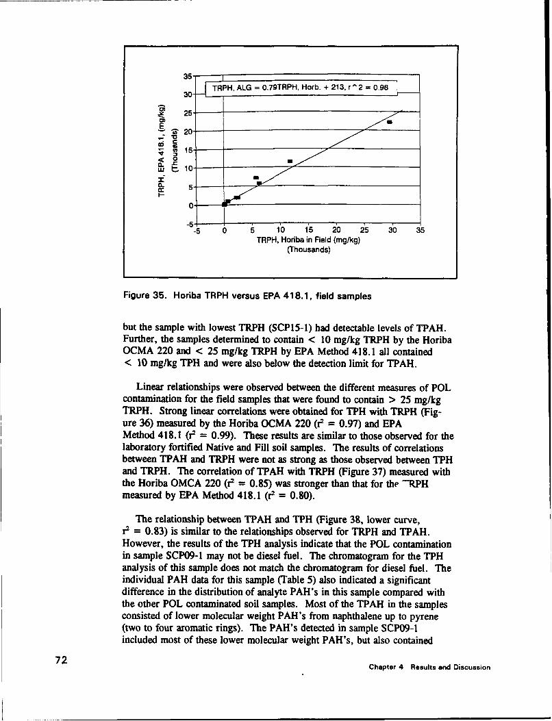
35TRPH, ALG = 0.79TRPH, Horb. + 213, r 2 0.98
2-
C 6
-5 0 5 10 15 20 25 30 35
TRPH, Horiba in Field (mg/kg)(Thousands)
Figure 35. Horiba TRPH versus EPA 418.1, field samples
but the sample with lowest TRPH (SCP15-1) had detectable levels of TPAH.Further, the samples determined to contain < 10 mg/kg TRPH by the HoribaOCMA 220 and < 25 mg/kg TRPH by EPA Method 418.1 all contained< 10 mg/kg TPH and were also below the detection limit for TPAH.
Linear relationships were observed between the different measures of POLcontamination for the field samples that were found to contain > 25 mg/kgTRPH. Strong linear correlations were obtained for TPH with TRPH (Fig-ure 36) measured by the Horiba OCMA 220 (r2 = 0.97) and EPAMethod 418.1 (r2 = 0.99). These results are similar to those observed for thelaboratory fortified Native and Fill soil samples. The results of correlationsbetween TPAH and TRPH were not as strong as those observed between TPHand TRPH. The correlation of TPAH with TRPH (Figure 37) measured withthe Horiba OMCA 220 (i9 = 0.85) was stronger than that for the -RPHmeasured by EPA Method 418.1 (r2 = 0.80).
The relationship between TPAH and TPH (Figure 38, lower curve,r2 = 0.83) is similar to the relationships observed for TRPH and TPAH.However, the results of the TPH analysis indicate that the POL contaminationin sample SCP09-1 may not be diesel fuel. The chromatogram for the TPHanalysis of this sample does not match the chromatogram for diesel fuel. Theindividual PAH data for this sample (Table 5) also indicated a significantdifference in the distribution of analyte PAH's in this sample compared withthe other POL contaminated soil samples. Most of the TPAH in the samplesconsisted of lower molecular weight PAH's from naphthalene up to pyrene(two to four aromatic rings). The PAH's detected in sample SCP09-1included most of these lower molecular weight PAH's, but also contained
72 Chapter 4 Results and Discussion

TRPH, Horb. = 1.8OTPH - 1065.9, r 2 = 0.97
25
20
15-
:e 0 10-
5-
04 TRPH, ALG= 1.39TPH -78.5. r2 =0.99
.-5"0 2 4 8 10 1'2 1'4 1'6 18
TPH, (mg/kg)(Thousands)
C EPA41,l Hob aOCMA,220o- EPA.,41.1 - HomonCMAW22o]
Figure 36. TPH versus TRPH, field samples
significant amounts of the higher molecular weight PAH's (Table 5). TheTPH chromatogram suggested that the POL might be a lubricating oil orheavier fuel oil. Another explanation for the difference in PAH distributionfor this sample compared with the others is that this sample may represent anolder fuel spill and the PAH distribution is the result of aging. The correla-tion between TPAH and TPH is significantly improved (r2 = 0.93) when thedata for sample SCP09-1 is excluded from the correlation (Figure 38). Thisimproved correlation, combined with the TPH chromatographic profile indica-tive of a POL type other than diesel fuel, suggest that a knowledge of fueltype is required before conclusions can be drawn from correlations betweenLIF response and POL contaminant concentration.
Laser induced fluorescence as a quantitative measure of POLcontamination
The 22 soil samples obtained for validation of the SCAPS POL sensorwere analyzed in the field for LIF response in a manner analogous to theprocedure used to analyze the laboratory-fortified soil samples. It should benoted that this procedure included normalizing the soil sample LIF response tothe response of a Rhodamine standard solution analyzed before and zfter thesoil sample. The LIF response of the soil samples summarized in Table 4includes both Rhodamine normalized and raw LIF data. As discussed earlier,some of these samples were determined to be false positive samples for POL(yielding LIF sensor response, but analytical results (TRPH) indicated no POLcontamination). The samples that were determined to contain POL
73Chapter 4 Results and Discussion

35
30•• TRPH, Horb. = 408TPAH + 1380, r^2 = 0.85
25-
E5 15:e 0
5TRPH, ALG = 302TPAH + 1990, r 2 = 0.80
0,
0 1,0 2o 30 4 o 60o 70TPAH, (mg/kg)
C EPA41.1 N H'qib~OCMA220- EPA418.1 - HonbaOCMA220
Figure 37. TPAH versus TRPH, field samples
18
1614 TPH = 225.2TPAH +1999, r ^2 = 0.93
12o~10-
6--
4 3 PTP=e220.4TPAHr+u1447,rf2e=l0.83
2-4
0o , io 2 3b 4,0 50 6 70TPAH, (mg/kg)
-all data -omit SCIPO9-1 x SCIPO9-1
Figure 38. TPAH versus TPH, field samples
contamination by TRPH, TPH, and TPAH analyses also yielded positive LIFresponse (Table 4).
Linear relationships were observed for the cc. relation of LIF response withall three POL parameters used as measures of soil contamination. The soilsample fluorescence correlated with the TRPH measured in the field with theHoriba OCMA 220 (Figure 39) and TRPH measured by EPA Method 418.1
74 Chapter 4 Results and Discussion

600 A
500- Fluor. = 0.0125TRPH + 191.5, r"2 = 0.88
o 400-
O 300" A
S200-0o . A
100 E. 10" -Fluor. = O.O084TRPH + 159.9, r"2 = 0.77
00 5 10 15 2b 25 30
TRPH, Horiba (mg/kg)(Thousands)
FIE�njo BA raflum. - nwnjrm. flu O
Figure 39. TRPH, Horiba versus fluorescence
(Figure 40). It is interesting to note that the correlation of LIF response withTRPH (by both Horiba OCMA 220 and EPA Method 418.1) is stronger forthe raw LIF response (Figure 39, r2 = 0.88 and Figure 40, r2 = 0.78)) thanfor the normalized fluorescence data (Figure 39, r2 = 0.77 and Figure 40,r2 = 0.70). These data suggest that the Rhodamine normalization proceduremay introduce bias into the LIF response data.
The raw fluorescence response of the soil samples is also correlated morestrongly with the other two parameters (TPH and TPAH) used to measurePOL contamination in this study. The raw fluorescence was correlated withthe TPH at r2 = 0.80, while the normalized fluorescence correlated with TPHat r2 = 0.70 Figure 41). Very similar results were obtained for the relation-ship between TPAH with both the raw and normalized fluorescence (Fig-ure 42, r2 = 0.81 and 0.72, respectively).
Validity of laboratory calibration of SCAPS POL sensor
The linear relationships observed for the SCAPS POL sensor LIF responsewith each of the three different parameters used to verify POL contaminationin both field and laboratory fortified samples illustrate the potential efficacy ofLIF for in situ detection of POL contamination. These same data also point tosome potential limitation of this technology that must be defined and under-stood before the full benefits of the SCAPS POL sensor can be realized.
The lower slopes of the Fill versus the Native laboratory-fortified soils forthe regressions of the LIF response with each of the POL parameters
75Chapter 4 Results and Discussion
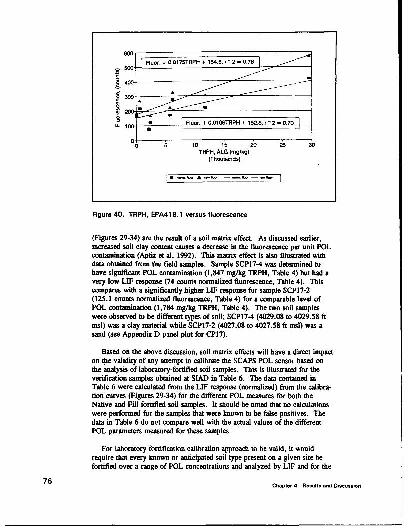
500 __[.Fluor. =0.01 75TRPH + 154-5, r ^2 =0.78
0 400-
300 -
0
" 1 0 Fluor. + 0.0106TRPH + 152.8. r"2 = 0.70U-100 -
010 1'0 15 20 25 30TRPH, ALG (mg/kg)
(Thousands)
m om. Sm.~ A mw flu. - nom. 0".e - r"w flu
Figure 40. TRPH, EPA418.1 versus fluorescence
(Figures 29-34) are the result of a soil matrix effect. As discussed earlier,increased soil clay content causes a decrease in the fluorescence per unit POLcontamination (Aptiz et al. 1992). This matrix effect is also illustrated withdata obtained from the field samples. Sample SCP17-4 was determined tohave significant POL contamination (1,847 mg/kg TRPH, Table 4) but had avery low LIF response (74 counts normalized fluorescence, Table 4). Thiscompares with a significantly higher LIF response for sample SCP17-2(125.1 counts normalized fluorescence, Table 4) for a comparable level ofPOL contamination (1,784 mg/kg TRPH, Table 4). The two soil sampleswere observed to be different types of soil; SCP17-4 (4029.08 to 4029.58 ftmsl) was a clay material while SCP17-2 (4027.08 to 4027.58 ft msi) was asand (see Appendix D panel plot for CP17).
Based on the above discussion, soil matrix effects will have a direct impacton the validity of any attempt to calibrate the SCAPS POL sensor based onthe analysis of laboratory-fortified soil samples. This is illustrated for theverification samples obtained at SIAD in Table 6. The data contained inTable 6 were calculated from the LIF response (normalized) from the calibra-tion curves (Figures 29-34) for the different POL measures for both theNative and Fill fortified soil samples. It should be noted that no calculationswere performed for the samples that were known to be false positives. Thedata in Table 6 do not compare well with the actual values of the differentPOL parameters measured for these samples.
For laboratory fortification calibration approach to be valid, it wouldrequire that every known or anticipated soil type present on a given site befortified over a range of POL concentrations and analyzed by LIF and for the
76 Chapter 4 Results and Discussion
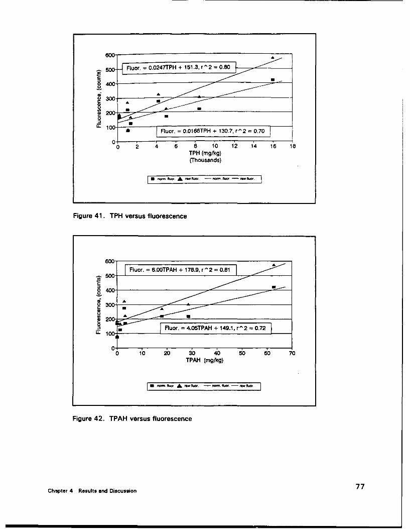
600O
50- Fluor. = 0.0247TPH + 151.3, r^2 = 0.80
0 400 "
2?200-0
u. 100 IFluor. = 0.0166TPH + 130.7, r-2 = 0.70
010 2 4 6 8 10 12 14 16 18
TPH (mg/kg)(Thousands)
*nom. &wu. mw Suwi. - noqm. fiutm nwio
Figure 41. TPH versus fluorescence
600S 00- Fluor.=6.00TPAH +178.9, rý2 = 0.81 • A"
3500.-
o 00-
- Fluor. =4.05TPAH + 149.1, r72 =072" 100
0 10 20 30 40 0 60 70TPAH (mg/kg)
%W., fuc A mwflw omfur mwfl&wr
Figure 42. TPAH versus fluorescence
Chapter 4 Results and Discussion 77

Table 6Comparison of Predicted POL based on Laboratory Calibrations with MeasuredPOL
Native Calibration Fill Calibration Actual Measured Values
Sample TRPH TPAH TPH TRPH TPAH TPH TRPH TPAH TPHName mg/k9 mg/kg mg/kg mg/k mg/kg J mg/kg mg/kg mg/kg m9/kg
SCP14-1 -1331.1 -2.1 -1350 -323.9 -8.6 -324.5 203.2 <0.41 200
SCP14-2 4128.8 7.7 4040.7 11506.0 274.3 12847 22151 62.9 16000
SCP14-3 -224.6 -0.1 -257.6 2073.5 48.7 2344.8 11445 28.6 8420
SCP17-1 -1255.3 -1.9 -1275 -159.6 -4.7 -141.6 7228 3.29 5040
SCP17-2 -2207.1 -3.6 -2215 -2221.9 -54.0 -2438 1784 1.25 1360
SCP09-1 -223.9 -0.1 -256.9 2075.0 48.7 2346.4 845.9 17.97 1060
SCP17-3 1010.0 2.1 961.32 4748.4 112.7 5323 5817 3.03 4250
SCP17-4 -3300.1 -5.6 -3294 -4590.0 -110.7 -5074 1847 <0.41 1070
POL parameters of interest. These different calibration curves could then beused to convert the LIT response obtained on field pushes to a quantitativemeasure of POL contamination, depending on the soil type indicated at anygiven depth. The cost of obtaining, construction and analyzing the fortifiedsoil samples for a single soil type are non-trivial ($17,000 analytical cost forTRPH, TPH and TPAH).
Implications of in-field measurement of TRPH for SCAPS POL sensorverification and calibration
The results from the onsite determination of TRPH in SIAD soil samplesusing the Horiba OCMA 220 combined with the strong correlation betweenthese data and the TRPH data and the TRPH measured by WES using EPAMethod 418.1 (Figure 35) illustrate two important advantages of onsite deter-mination of POL contamination as an adjunct to the LIT data provided by theSCAPS POL sensor. First, the Horiba OCMA 220 provided rapid identifica-tion of potential false positive LIW responses of the SCAPS POL sensor.Identification of false positive SCAPS POL sensor response based on labora-tory TRPH measurement of field samples generally takes weeks to obtain.
Another important benefit of the onsite determination of POL -.ontamina-tion is the verification of true positive SCAPS POL sensor LIT responses.The eight soil samples obtained at SIAD that were determined in the field tocontain > 15 mg/kg TRPH (Table 4) exemplify the utility of this approach totimely verification of SCAPS POL sensor response. This type of informationwill also assist the site engineer in decisions about where to sample to charac-terize POL contamination. An important additional use of this technology isthe use of a field portable TRPH detector to verify true negative LIT response
78 Chapter - Results and Discussion

and determination of POL contamination at detection levels below the sensitiv-ity of the SCAPS POL sensor.
The results of the correlations between LIF response and the TRPH dataobtained in the field (Figure 39) illustrate the potential utility of this techniquefor onsite calibration of the SCAPS POL sensor. Calibration using actualcontaminated soil has the advantage that the matrix effects due to soil prop-erties should be implicit in the samples. For example, the SCAPS soil classi-fication could be used to identify soil-type matrix effects. Also, fuel-agingeffects for a particular spill should not cause the bias often encountered withlaboratzry calibration (using fresh fuel).
The use of a field portable instrument like the Horiba OCMA 220 wouldnot completely replace laboratory analysis of field samples for SCAPS POLsensor verification. Standard quality control practices require verification ofsome portion (generally 10 percent) of samples analyzed. If normal QC prac-tices are followed, every tenth sample analyzed in the field for POLcontamination using a field portable instrument would have to be verified bylaboratory analysis.
The onsite verification of LIF "false positives" enabled the development ofthe three-dimensional model visualization of the contaminant "plume" shownpreviously in Figures 15 through 22. The use of the Horiba OCMA 220 todifferentiate the POL LIF response for the mineral fluorescence is an impor-tant improvement in the onsite verification of the SCAPS POL LIF sensor.However, the use of the fluorescence emission spectra collected in the normalSCAPS LIF penetration to differentiate POL fluorescence from mineralfluorescence may be possible. The spectral signatures of the POL fluores-cence at SIAD were significantly different from the mineral fluorescencesignatures (Figure 43). The POL fluorescence peaked in the 400-nm rangewhile the mineral fluorescence peaked in the 450-nm region of the fluores-cence emission spectra. The emission profiles for the POL and mineralfluorescence are also quite different.
79Chapter 4 Results and Discussion

S ECO
1PCI
0
ct CL
0
.-i
0 S
so Chapter 4 Results andDsuso
5 Summary, Conclusions, andRecommendations
Summary
The SCAPS visited the SIAD Diesel Spill Area near Building 403 (approxi-mately 5 acres in area) during the period 28 September through 15 October1993. The objectives of the SCAPS investigation are summarized below:
Objectives
a. Collect and interpret penetrometer sensor data. A total of 22 penetra-tions were accomplished for this purpose. The locations had beenpredesignated, but minor adjustments were made to accommodate thetruck accessibility and to provide better spatial distribution of datapoints. The depth limitations caused by the soil resistance to penetra-tion restricted most of the penetrations to depths above the groundwatertable. The data collected were analyzed and postprocessing 3-D visual-ization technology enabled large scale interpretations for soil stratigra-phy patterns and soil fluorescence patterns.
b. Collect subsurface soil and groundwater samples for analysis by theAEC site environmental contractor, Montgomery Watson, Inc. Fivesoil sample sets and one groundwater sample were collected. The depthlimitations played a major role in this objective, especially for ground-water sampling. The inability of the groundwater samplers to penetratesignificantly below the groundwater surface elevation was a limitationfor SCAPS at this site.
c. Collect subsurface soil samples for fluorescence and soil classificationverification efforts. A total of 22 soil samples were retrieved for subse-quent field laboratory and WES laboratory analyses. Since the targeteddepths were relatively shallow (coincidental with soil fluorescence activ-ity), this objective was fully achieved. The results of the in-field labo-ratory validation studies provided insight into the capabilities of theSCAPS POL (LIF) sensor for in situ detection of POL contamination.The use of a field portable instrument for TRPH determination
Chapter 5 Summary, Conclusions, and Recommendations 81

demonstrated the potential utility of onsite verification of LIF response.The identification of false positive LIF response due to fluorescingminerals was illustrated. The onsite determination of false positiveSCAPS POL sensor response will allow the project engineer to makemore informed decisions about the location of contamin&,ts at the site.The strong correlation between the Horiba OCMA 220 and EPAMethod 418.1 TRPH results for field soil samples obtained at the SIADsupport the efficacy of the in-field determination of POL contaminationwith this technology. The correlations observed between theHoriba OCMA 220 TRPH measurements and the SCAPS POL sensorLIF response illustrated the potential for onsite POL sensor LIFcalibration.
d. Continuation of the SCAPS field activities demonstration phase. All theSCAPS systems involving the above objectives were demonstrated atthis site. The 1.75-in. diam pushpipe was demonstrated at this site.The depth limitations previously discussed constituted the primary chal-lenge for SCAPS system improvements. Other challenges for improve-ment were also noted.
Conclusions
Soil classification and fluorescence
Soil classifications based on visual and laboratory analyses closely matchedthose indicated by the in situ sensor probe. The predominant soil type wassand (fine to coarse gradations) with interbedded finer-grained silts and clays.Sands provided the greatest penetration resistance, and their physical attributes(matrix structure, particle size, shape, and strength properties) were responsi-ble for the relatively shallow depths (less than 68 ft) achieved by the pene-trations at this site.
Soil fluorescence response was observed at depths above approximately20-ft bgs. It was interesting to note that the fluorescence occurred within ornear the previously excavated and backfilled area immediately south of theBuilding 403 mechanical room, and at a separate location south of the oldBoiler Plant (Building 402). No fluorescence was observed at deeper depthswithin the "smear zone" just above the water table elevation (approximately62-ft bgs). A larger number of penetrations into the water table aquifer wouldhave served to identify the presence (or absence) of POL contaminants atthose depths, but, as previously discussed, were not possible.
The presence of fluorescence response interference (due to calcite minerals)was not entirely unanticipated due to the significant geological history of theSIAD area. This site was the second SCAPS site visited west of the Missis-sippi River, and the first site in the Great Basin and Range physiographicalregion west of the Rockies. The diverse geology (volcanoes, earthquakes, and
82 Chapter 5 Summary, Conclusions, and Recommendations
various depositional and erosional patterns) of this area increased thepossibility of encountering challenging subsurface conditions.
Sampling efforts
The Mostap' soil sampler is well-suited for relatively shallow sampling toapproximately 20-ft bgs (in similar subsurface environments). The Gouda"soil sampler is better suited for deeper penetrations, but its internal volumedoes not allow a sample size large enough for standard laboratory analysis.
The Hydropunch'TM Model I penetrates deeper than the Model II, but itsinternal volume does not allow for an adequate sampling size. It offers oneadvantage in that it may be lowered into the same penetration hole repetitively(if operational care is taken to prevent premature engagement). The Model IIexpendable tip prevents repetitive sam: ,ing in the same hole. If the targeteddepth may be reached without repetitive attempts, the Model II is the pre-ferred choice.
Sampling verification
The data presented in Table 6 support the conclusion that the use of labora-tory fortified soil samples for calibration of the SCAPS POL sensor for fielddetermination of POL concentrations may be of only limited utility. Based onthe cost of laboratory fortified samples, the laboratory fortification calibrationapproach is probably not feasible for multiple soil types at a given site or acomplex stratigraphy at a site to be characterized using the SCAPS POLsensor.
The validation data obtained at SIAD from field soil samples indicate thatthere is a relationship between the intensity of the SCAPS POL sensor LIFsensor response and soil POL contamination, when soil matrix effects aretaken into account. Although the field verification sampling uncovered thepresence of "false positives" (fluorescent minerals), no instance of non-fluorescing (above a normal background fluorescence level) POL contamina-tion was observed. All POL ccrnamination observed in field and laboratoryanalysis also indicated fluorescence responses. Knowing the locations of"false fluorescence" responses (i.e. fluorescent mineral layers) enabled a moreaccurate 3-D modeling visualization of the contaminant plume. T'he datapresented in Figure 43 indicate that differentiation of POL and mineral fluo-rescence based on LIF profiles may be possible.
SCAPS demonstration
The soil penetration resistance provided the major challenge at this site and(as previously discussed) was a function of the soil type. The capability of theSCAPS truck to achieve deeper penetrations while pushing through sand lay-ers with a cone tip resistance between 200 to 400 tons/ft has already been
83Chapter 5 Summary, Conclusions, and Recorimei.vations
demonstrated (for example, at a Coastal Plain site where depths down to150 ft bgs were reached prior to "refusal" (Koester et al. 1993a)). However,the larger diameter (1.75 in.) pushpipe had not been used prior to the SIADsite investigation, and it was concluded that improvements are needed if it isto achieve depths similar to the normally-used smaller diameter (1.4 in.)pushpipe.
Recommendations
Site specific
The presence of remnant hydrocarbon contamination was confirmed, basedon the probe fluorescence sensor and verification sampling. Additional soilsampling at deeper depths near the water table elevation and additionalgroundwater samples are needed to determine the extent of contaminant trans-port (if any). In addition to the POL contamination observed south of Build-ing 403, the presence of a separate source south of Building 402 may warrantfurther investigation. Soil and groundwater monitoring efforts should betargete', in the area between Buildings 402 and 403.
SCAPS system
Additional development is needed to enhance methods for increasing pene-tration depth. Specifically, friction breakers, air injection, and/or other tech-niques must be tested with the pushpipe, the sensor probe, and the samplerunits in order to overcome penetration resistance forces.
Methods and equipment to improve the capabilities of the support systemsare needed. Specifically, the grout system needs to be tailored for full opera-tional capability during inclement weather, i.e. it needs to be weatherproofedagainst wet and cold conditions. Improved methods for sampler cleaning areneeded. A method to ensure true vertical alignment of the pushpipe at theground surface is needed. Incorporation of a Global Positioning System sur-veying system will increase the efficiency and capabilities of the data process-ing system.
The SIAD validation study was a strong step in the validation of theSCAPS POL sensor. Additional site investigations with onsite verification ofSCAPS POL sensor LIF response with field portable POL instrumentation isrequired before the general applicability of the findings reported here can beconfirmed. A larger database that includes many different fuel and soil typesis needed to better define the capabilities of this new technology for determi-nation of POL contamination. Further investigation of mineral fluorescencesignatures should be carried out to determine the feasibility of differentiationof POL and mineral fluorescence based solely on emission profiles. Incorpo-ration of onsite 3-D visualization capability integrated with onsite verification
84 Chapter 5 Summary, Conclusions. and Recommendations
procedures will enhance the efficiency of contaminant plume identification andspatial location.
85Chapter 5 Summary. Conclusions, and Recommendations

Bibliography
Apitz, S. E., Brobridge, L. M., Theriault, G. A., and Lieberman, S. H.(1992). "Remote in situ determination of fuel products in soils: filedresults and laboratory investigations." Analusis, Vol. 20, pp. 461-474.
Benioff, P., Filley, T., and Tsai, S. Y. (1988). "Master Environmental Planfor the Sierra Army Depot," October 1988.
Bowles, J. E. (1988). "Foundation Analysis and Design," 4th Edition.McGraw-Hill, Inc., New York.
Dana, J. D. (1959). Dana's Manual of Mineralogy," 17th Edition. JohnWiley and Sons, Inc., New York.
Handman, E. H., Londquist, C. J., and Maurer, D. K. (1990). "Groundwa-ter Resources of Honey Lake Valley, Lassen County, California, andWashoe County, Nevada," USGS Water-Resources InvestigationsReport 90-4-5.
Koester, J. P., Lee, L. T., Olsen, R. S., Douglas, D. H., Comes, G. D.,Cooper, S. S., and Powell, J. F. (1993a). "Field Trials of the Site Char-acterization and Analysis Penetrometer System at the Savannah River Site(SRS)." Technical Report GL-93-16. U.S. Army Engineer WaterwaysExperiment Station, Vicksburg, MS.
Koester, J. P., Lee, L. T., Powell, J. F. and Goodson, R. (1993b). "Opera-tions Manual for the Site Characterization and Analysis Penetrometer Sys-tem," (in preparation) U.S. Army Enginee.- Waterways Experiment Station,Vicksburg, MS.
Lee, L. T., Chrestman, A. M., Douglas, D. H., Powell, J. F., and Malone,P. G. (1993). "Site Investigations with the Site Characterization andAnalysis Penetrometer System at Fort Dix, New Jersey." TechnicalReport GL-93-17. U.S. Army Engineer Waterways Experiment Station,Vicksburg, MS.
86Bibliography
Lee, L. T., and Powell, J. F. (1993). "Use of the Site Characterization andAnalysis Penetrometer System at the Walnut Creek Watershed, Ames,Iowa." Miscellaneous Paper GL-93-12. U.S. Army Engineer WaterwaysExperiment Station, Vicksburg, MS.
Mitchell, J. K. (1976). "Fundamentals of Soil Behavior." John Wiley &Sons, Inc., New York.
Montgomery Watson, Inc. (1993). "Sierra Army Depot Group I RemedialInvestigation/Feasibility Study, Draft Final," Prepared for USATHAMA,Aberdeen Proving Ground, Maryland, April 1993.
Puppala, A. J., Acar, Y. B., and Senneset, K. (1993). "Cone Penetration inCemented Sands: Bearing Capacity Interpretations," American Society ofCivil Engineers Journal of Geotechnical Engineering, Vol. 119, No. 12,December 1993, pp. 1990-2001.
Sharp, M. K., Kala, R., and Powell, J. F. (1992). "Use of the Site Charac-terization and Analysis Penetrometer System at the Grandville SuperfundSite, Grandville, Michigan." Miscellaneous Paper GL-92-38. U.S. ArmyEngineer Waterways Experiment Station, Vicksburg, MS.
Sharp, M. K., Olsen, R. S., and Kala, R. (1992). "Field Evaluation of theSite Characterization and Analysis Penetrometer System at the PhiladelphiaNaval Shipyard, Pennysylvania." Miscellaneous Paper GL-92-39.U.S. Army Engineer Waterways Experiment Station, Vicksburg, MS.
U.S. Army Toxic and Hazardous Materials Agency (USATHAMA). (1979)."Installation Assessment of Sierra Army Depot, Report No. 149"; Aber-deen Proving Ground, Maryland, December 1979.
U.S. Department of Agriculture. (1917). "Soil Survey of the Honey LakeArea, California." Washington, DC: Government Printing Office.
U.S. Environmental Protection Agency. (1984). "Test Methods for Evaluat-ing Solid Waste; Physical/Chemical Methods," SW-846 Third Edition.U.S. EPA, Washington, DC.
U.S. Department of Transportation. (1978). "Guidelines for Cone Penetra-tion Testing, Performance, and Design." Publication No. FHWA-TS-78-209. Washington, DC: Federal Highway Administration.
87Bibliography

Appendix AStandard Practice forPreparation of Calibration SoilSamples for the SCAPS Laser-Induced Fluorescence Sensor
AlAppendix A Standard Practice for Preparation of Calibration Soil Samples

STANDARD PRACTICE FOR THE PREPARATION OF CALIBRATION SOIL SAMPLES
FOR THE SCAPS LASER INDUCED FLUORESCENCE DETECTOR
1. SCOPE
1.1 This proctice establishes uniform procedures for thedevelopment, preparation, and use of soil samples for thecalibration of the SCAPS laser-induced fluorescence (LIF)detector. The LIF detector calibration will be oriented towardthe evaluation of semi-volatile compounds that are most commonlyfound at military sites requiring cleanup.
1.2 calibration samples are prepared using soil samplesthat best represent the soil type(s) found at the site. Thisenables the calibration procedure to compensate for any matrixeffects found in the soil samples. Whenever possible,calibration soils should be spiked with the pure products (i.e.diesel, kerosene, jet fuel, etc.) taken from the site toeliminate any manufacturing differences.
1.3 This standard may involve hazardous materials,operations, and equipment. This standard does not purport toaddress all of the safety problems associated with its use. Itis the responsibility of the user of this standard to establishappropriate safety and health practices.
2. REFERENCED DOCUMENTS
2.1 ASTM STANDARD D-3975, PRACTICE FOR PREPARATION OFSAMPLES FOR COLLABORATIVE TESTING OF METHODS FOR ANALYSIS OFSEDIMENTS
3. SUMMARY OF PRACTICE
3.1 Soil samples of adequately defined composition andhomogeneity are required for calibrating the LIP detector forfield use with the SCAPS system. The ideal calibration systemwould utilize naturally contaminated soils at variousconcentrations to measure the quantitative responses of thesystem. Since this is not a feasible option, soils must beadequately prepared to ensure homogeneous spiking ofcontaminants. The soil must be ground to a standard particlesize to eliminate the settling out of denser particles therebychanging the concentration of contaminants in the calibrationsamples.
3.2. Samples spiked at several concentrations spanning theexpected concentration range are prepared to test the linearityof the system. Samples will also be analyzed by a provenlaboratory method to insure the bias and precision of the spikingtechnique. Samples will also be analyzed over time to test thestability of the spiked compounds in the soil matrix.
A2 Appendix A Standard Practice for Preparation of Calibration Soil Samples

4. SIGNIFICANCE AND USE
4.1 The objective of this practice is to provide guidelinesfor the preparation of soil samples for use in calibrating theLIF detector for use with the SCAPS and for determining theprecision and bias associated with the process.
5. PREPARATION OF CALIBRATION SAMPLES
5.2 In preparation of the soil samples for grinding, thesamples are cleaned of any vegetation, large rocks, or otherextraneous materials. At this point, the percent moisture in thesample is measured to enable the adding back of moisture to thesample to represent the field situation. A sufficient quantityof soil to produce approximately 10 Kg of dry soil is is ovendried at 1060C for 18 hours in a vented oven. After cooling, thesample is ground using a Brinkmann Model ZM-I centrifuged grinderat 20000 rpm to a particle size of less than 0.5 micron. Theground soil is collected in a 5-gallon glass carboy and tumbledfor 18 hours to ensure homogeneous soil for spiking. Aliquotsweighing one thousand ±0.2 grams are weighed into h gallon pre-cleaned glass jars with teflon-lined lids.
5.3 Calibration samples are prepared in concentrations of0, 100, 300, 500, 1000, 2000, 5000, and 10000 mg/kg using thesite contaminant(s). The 1000 gram calibration samples at eachlevel provide sufficient material for triplicate analysis bylaboratory methods and by LIF to assess precision and accuracy.The calibration samples are prepared by spiking each of the 1000gram ground site soil samples with 0, 100, 300, 500, 1000, 2000,5000, and 10000 mg of contaminant(s). The contaminant spikes aredistributed as uniformly as possible over the surface of thesoil. The spiked soils are tumbled for 92 hours to ensurehomogeneous distribution and equilibration of the contaminantthroughout the soil particles. Based on the previouslydetermined moisture content, reagent water is added to each ofthe individual samples and tumbled for an additional 72 hours.
A3Appendix A Stadard Practice for Preparation of Calibration Soil Samples

Appendix BSurveying Data
Appendix B Surveying Data Bi
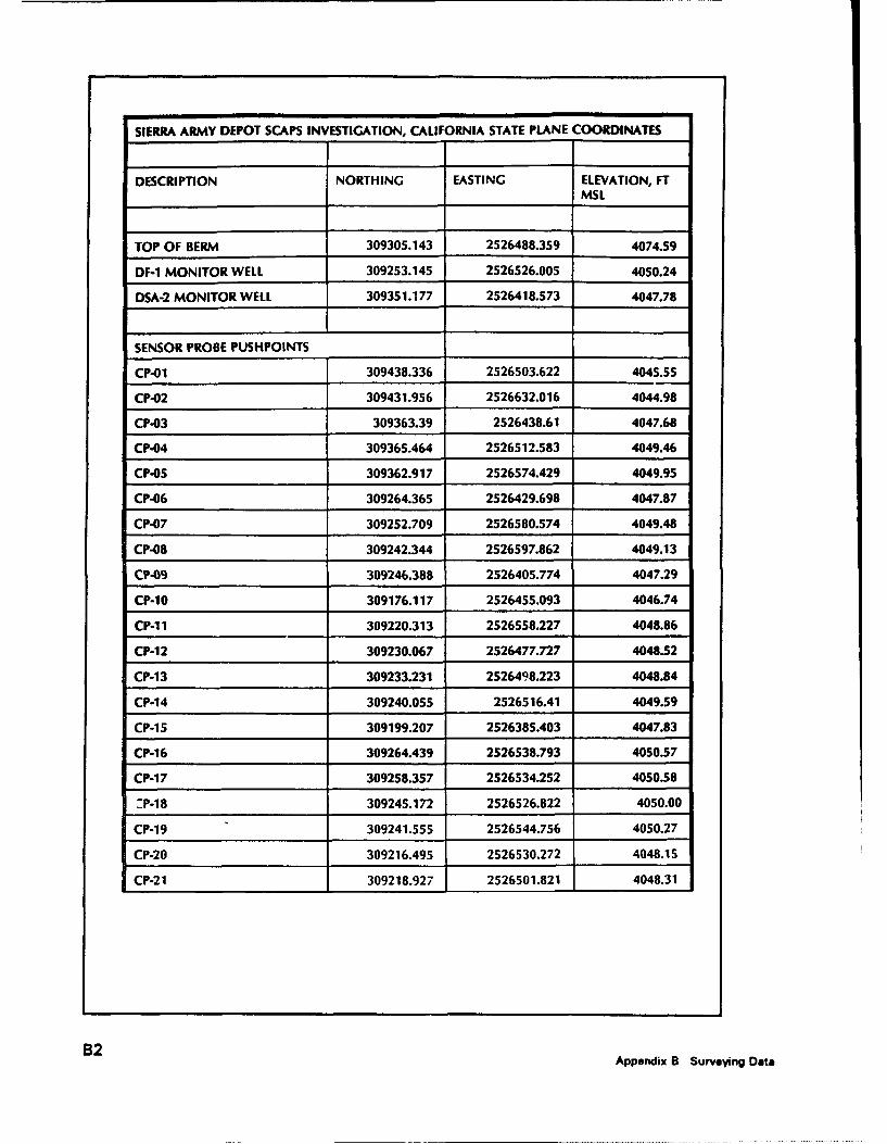
SIERRA ARMY DEPOT SCAPS INVESTIGATION, CALIFORNIA STATE PLANE COORDINATES
DESCRIPTION NORTHING EASTING ELEVATION, FTMSL
TOP OF BERM 309305.143 2526488.359 4074.59
DF-1 MONITOR WELL 309253.145 2526526.005 4050.24
DSA-2 MONITOR WELL 309351.177 2526418.573 4047.78
SENSOR PROBE PUSHPOINTS
CP-01 309438.336 2526503.622 4045.55
CP-02 309431.956 2526632.016 4044.98
CP-03 309363.39 2526438.61 4047.68
CP-04 309365.464 2526512.583 4049.46
CP-05 309362.917 2526574.429 4049.95
CP-06 309264.365 2526429.698 4047.87
CP-07 309252.709 2526580.574 4049.48
CP-08 309242.344 2526597.862 4049.13
CP-09 309246.388 2526405.774 4047.29
CP-10 309176.117 2526455.093 4046.74
CP-1 1 309220.313 2526558.227 4048.86
CP-12 309230.067 2526477.727 4048.52
CP-13 309233.231 2526498.223 4048.84
CP-14 309240.055 2526516.41 4049.59
CP-15 309199.207 2526385.403 4047.83
CP-16 309264.439 2526538.793 4050.57
CP-17 309258.357 2526534.252 4050.58
-P-18 309245.172 2526526.822 4050.00
CP-19 309241.555 2526544.756 4050.27
CP-20 309216.495 2526530.272 4048.15
CP-21 309218.927 2526501.821 4048.31
B2 Appendix 8 Surveying Data
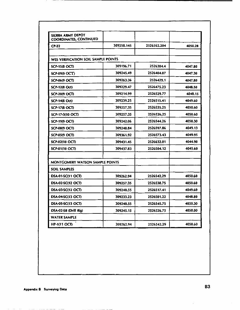
SIERRA ARMY DEPOTCOORDINATES, CONTINUED
CP-22 309258.145 2526562.204 4050.28
WES VERIFICATION SOIL SAMPLE POINTS
SCP-15(8 OCT) 309196.71 2526384.4 4047.80
SCP.09(9 OCT) 309245.49 2526404.07 4047.30
SCP-06(9 OCT) 309263.36 2526429.1 4047.80
SCP-12(8 Oct) 309229.47 2526475.23 4048.50
SCP-20(9 OCT) 309214.99 2526529.77 4048.15
SCP-14(8 Oct) 309239.25 2526515.41 4049.60
SCP-17(8 OCT) 309257.35 2526535.25 4050.60
SCP-17-3(10 OCT) 309257.35 2526536.25 4050.60
SCP-19(9 OCT) 309242.06 2526544.26 4050.30
SCP-08(9 OCT) 309240.84 2526597.86 4049.13
SCP-05(9 OCT) 309361.92 2526573.43 4049.95
SCP-02(10 OCT) 309431.45 2526632.01 4044.90
SCP-01(10 OCT) 309437.83 2526504.12 4045.60
MONTGOMERY WATSON SAMPLE POINTS
SOIL SAMPLES
DSA-01-SC(11 OCT) 309262.94 2526542.29 4050.60
DSA-02-SC(12 OCT) 309257.35 2526538.75 4050.60
DSA-03-SC(12 OCT) 309240.55 2526517.41 4049.60
DSA-04-SC(13 OCT) 309233.23 2526501.22 4048.80
DSA-05-SC(13 OCT) 309240.55 2526545.75 4050.30
DSA-02-SB (Drill Rig) 309245.15 2526526.75 4050.00
WATER SAMPLE
HP-1(11 OCT) 309262.94 2526542.29 4050.60
Appendix B Surveying Data B3

Appendix CSCAPS Field Sampling StandardOperating Procedure
Appendix C SCAPS Field Sampling Standard Operating Procedure C1
SCAPS Field Sampling Standard Operating Procedures
General
The intention of penetrometer sampling operations is to obtain a representative sampleof the candidate solid or liquid for laboratory analysis to determine the type andconcentration of contaminants present. Three different types of sampling are potentiallynecessary with any particular SCAPS site investigation. These three types of samplinginclude:
(1) pre-deployment sampling of contaminated soil and free POL. In addition,uncontaminated soil should be obtained for preparation of LIF laboratory calibration samples.Procedures for preparation of laboratory calibration sample will be discussed in detail later.
(2) field samples for laboratory verification of a minimum of 10% of LIFpositive SCAPS pushes during SCAPS site investigations.
(3) regulatory samples for laboratory analysis for regions of the site wherePOL contamination is below the detection limit for the LIF sensor for the POL/soil matrix ofinterest at a particular site.
Although only the type (3) samples will generally be of direct regulatory interest, all SCAPSsampling procedures will follow those specified by EPA in Test Methods for Evaluation ofSolid Waste. In addition, all SCAPS samples will be subject to a standard chain of custodysample tracking procedure.
The SCAPS is equipped with special penetrometer devices to obtain samples of soiland water at depths within the limit of current system performance. The devices are notdesigned to acquire any penetration resistance data, nor are they capable of grouting the holeon withdrawal. Both soil and water samplers require dedicated penetration operations; the
be perd t ~ 4pth ~ at, the bPtww of aa pwb-A. This section begins with adiscussion of sample handling protocol for contaminated soil studies, as dictated by the issuesparticular to laboratory analysis to identify and quantify contaminants in soil.
0 W. The heater on the high-pressure washer should be turned down so that watersprayed to clean the outside of the soil or water sampler is cool. As the last push rodremoved from the ground is cleaned, the cleaner system should be flushed until the effluentis cool. Someone should watch the soil sampler as it is pulled from the ground and tell thepush room operator to stop spraying cleaning water before the open end of the sampler entersthe cleaning collar beneath the truck. The soil sample may be washed out if water is sprayedacross the open end of the sampler. After the soil or water sample has been removed fromthe sampler, the device should be disassembled and separately cleaned with water over anopen drum or other, suitable container so that the cleaning water may be collected and
C2 Appendix C SCAPS Field Sampling Standard Operating Procedure
disposed of as required by site officials.
Sample handling considerations
General. Once the sample has been collected using the SCAPS subsurface samplingequipment, it must be stored and preserved to maintain the chemical and physicai propertiesthat it possessed at the time of collection, to the extent physically possible. The sample type,type of containers and their preparation, possible forms of contamination, and preservationmethods are all items which must be thoroughly examined in order to maintain the integrityof the samples. The sampling procedure (including containers, preservation and holdingtimes) and required sample size are determined by the EPA Method that will be used foranalysis of the contaminates of interest at a particular site. This section discusses con-siderations which must be addressed in order to maintain a sample's integrity for contaminantanalysis. This information is excerpted in part (where indented) from EPA Test Methods forEvaluating Solid Waste, Volume IB: Laboratory Manual Physical/Chemical Methods.
Sample handling and preservation.
This section deals separately with volatile and semi-volatile organics. Refer to Table3-2 for recommended sample containers, sample preservation, and sample holding times.
Volatile organics. Standard, 40 ml glass screw-cap VOA vials with
Teflon-lined, silicone septa may be used for both liquid and solid samples.The vials and septa should be soap-and-water washed and then rinsed withdistilled deionized water prior to use. After the vials and septa have beenthoroughly cleaned, they should be placed in a muffle furnace and dried at 105oC for approximately one hour.
NOIT: Do not heat the septa for extended periods of time (i.e. more than onehour, because the silicone begins tD slowly degrade at 105 oC).
As an alternate, sample containers which have been previously cleaned to the desiredEPA specifications are commercially available (i.e I-Chem Protocol B, 300 series, orequivalent).
When collecting the samples, liquids and solids should be introducedinto the vials gently to reduce agitation which might drive off volatilecompounds. Liquid samples should be poured into the vial without introducingany air bubbles within the vial as it is being filled. If a sample preservative isrequired, it should be added at this time. Should bubbling occur as a result ofviolent pouring, the sample must be poured out and the vial refilled (NOTEFOR SCARS APPLICATION: the penetroinctr water saimpler does not affordthe luxury of unlimited liquid sample volume; the Hydropunch IT" devicedescribed later collects no more than 1.2 liters under the best of circumstances
exercise caution not to violate this procedure). Each VOA vial should be
Appendix C SCAPS Field Sampling Standard Operating Procedure C3
filled until there is a meniscus over the lip of the vial. The screw-top lid with
the septum (Teflon side towarý the sample) should then be tightened onto thevial. After tightening the lid, the vial should be inverted and tapped to check
for air bubbles. If there are any air bubbles present the sample must beretaken. Two VOA vials should be filled per sample locaTion.
VOA vials for samples with solid or semi-solid (sludges) matrice•should be completely filled to the extent possible. The vials shoulo , tappedslightly as they are filled to try and eliminate as much free air space aspossible. Two vials should also be filled per sample location.
VOA vials should be filled and labeled immediately at the point atwhich the sample is c~ollected. They should NOT. be filled near a runningmotor or any type of exhaust system beause dmcage fumes and vapors mayontaminate the smples. The two vials from each sampli le ,ocations should
then be sealed in separate plastic bags to prevent cross-contamination betweensamples particularly if the sampled waste is suspected of containing high levelsof volatile organics. (Activated carbon may also be included in the bags toprevent cross-contamination from highly contaminated amples). VOAsamples may also be contaminated by diffusion of volatile organics throughthe
C4Appendix C SCAPS Field Sampling Standard Operating Procedure

Table 3-2Required Containers, Preservation Techniques, and Holding Times (Excerpted inpart from Table 2-20; EPA Test Methods for Evaluating Solid Waste Vol 1B)
Name Containar' Preservation Sample Vokmw Maximium HoldingRequired Thmy
Oil and grease G Cool, 4oC, H2SO, to aqueous: 1 L 28 daysEPA Method 9071A pH<2 solid: 20-30 g
Total Recoverable G, Teflon-lined Cool, 4oC, HCI to aqueous: 1 L 28 daysPetroleum Hydrocarbons cap pH<2 solid: 20-30 g
EPA Method 418.1
Organic carbon,total PG Cool, 40C. H2SO, to 28 daysITOC) pH <2
Polynuclear aromatic G, Teflon-lined Cool, 4*C, 0.008% aqueous: I L 7 days until ex-hydrocarbons cap Na 2S.O 3 store in solid: 50-100 g traction, 40 days
dark after extraction
Chlorinated hydrocar- G, Teflon-lined Cool, 4oC 7 days untilbons cap extraction, 40
days after ex-traction
Volatile Organics
Water Samples 2 40-ml vials 4 drops conc. HCI, aqueous: 40 mL 14 dayswith Teflon Cool, 4oClined septum
Soil/Sediments and 4-oz (1 20-ml) Cool, 4oC solid: 50-80 g 14 daysSludges wide mouth
glass withEPA Method 8020 Teflon liner
Semi-volatile Organics,OrganochlorinePesticides. PCBs
Water Samples 1-gal. or 2 1/2- Cool, 4*C aqueous: I to 7 days untilgal. amber 2.5 gal. extraction, 40glass with days after ex-Teflon"' liner traction
Soil/Sediments and 8-oz. wide Cool, 40C solid: 50-100 g 14 days untilSludges mouth glass extraction, 40EPA Methods 8100 and with days after ex-
8270 Teflon"' liner traction
tPolrbylnec (P) or Glass (G)
Appendix C SCAPS Field Sampling Standard Operating Procedure C5

septum during shipment and storage. To monitor possible contamination, a trip blankprepared from distilled deionized water should ALWAYS be carried throughout thesampling, storage, and shipping process.
Semi-volatile organics (includes pesticides and herbicides). Containersused to collect samples for the determination of semi-volatile organiccompounds should be soap-and-water washed followed by methanol (orisopropanol) rinsing. The sample containers should be of glass or Teflon andhave screw-caps with Teflon lined septa. In situations where Teflon is notavailable, solvent-rinsed aluminum foil may be used as a liner. Highly acidicor basic samples may react with the aluminum foil, causing eventualcontamination of the sample. Plastic containers or:M4* m.jM *Visd f~idie storag of samlcs due to the possibility of sample o minatin OtW.plithalate ters, and. ot•erhydrocarbons within tihelst•c. Sample containersshould be filled with care so as to prevent any portion of the collected samplecoming in contact with the sampler's gloves, thus causing contamination.Samples should not be collected or stored in the presence of exhaust fumes. Ifthe sample comes in contact with the sampler (e.g. if an automatic sampler isused), run reagent water through the sampler and use as a field blank.
It should be noted that sample bottles are available commercially that have been
precleaned to EPA specifications (i.e. I-Chem Protocol B, series 300 or equivalent).
Safety
Safety should always be the primary consideration in the collection ofsamples. A thorough understanding of the waste production process as well asall of the potential hazards making up the waste should be investigatedwhenever possible. The site should be visually evaluated just prior tosampling to determine additional safety measures. i
Chain-of-custodyThe following information on chain of custody procedures is excerpted from EPA-
CLP SOW 390 (where indented). For application of this information to SCAPS siteinvestigations, the Contractor will refer to the WES SCAPS Team and the Laboratory willrefer to WES ECB.
A sample is physical evidence collected from a facility or from theenvironment. Controlling evidence is an essential part of the hazardous wasteinvestigation effort. To accomplish this, Contractors are required to develop
C6Appendix C SCAPS Field Sampling Standard Operating Procedure
and implement the following sample identification, chain-of-custody, samplereceiving, and sample tracking procedures.
Sample identification. To assure traceability of the samples while inpossession of the Contractor, the Contractor shall have a specified method formaintaining identification of samples throughout the laboratory.
Each sample and sample preparation container shall be labeled with theEPA number or a unique laboratory identifier. If a unique laboratoryidentifier is used, it shall be cross-referenced to the EPA number.
Chain-of-custody procedures. Because of the nature of the data beingcollected, the custody of EPA samples must be traceable from the time thesamples are collected until they are introduced as evidence in legalproceedings. The Contractor shall have procedures ensuring that EPA samplecustody is maintained and documented. A sample is under custody if:
"* It is in your possession, or
"* It is in your view after being in your possession, or
"* It was in your possession and you locked it up, or
"* It is in a designated secure area. (Secure areas shall beaccessible only to authorized personnel.)
Sample receiving procedures
The Contractor shall designate a sample custodian responsible for receiving all
samples.
The Contractor shall designate a representative to receive samples in the eventthat the sample custodian is not available.
The condition of the shipping containers and sample bottles shall be inspectedupon receipt by the sample custodian or his/her representative.
The condition of the custody seals (intact/not intact) shall be inspected uponreceipt by the sample custodian or his/her representative.
The sample custodian or his/her representative shall check for the presence orabsence of the following documents accompanying the sample shipment:
* Airbills or airbill stickers
Appendix C SCAPS Field Sampling Standard Operating Procedure
"* Custody seals
"* EPA custody records
"• EPA traffic reports or SAS packing lists
( Sample tags
The sample custodian or his/her representative shall sign and date all forms(e.g., custody records, traffic reports or packing lists, and airbills)accompanying the samples at the time of sample receipt.
The Contractor shall contact the Sample Management Office (SMO) to resolvediscrepancies and problems such as absent documents, conflicting information,broken custody seals, and unsatisfactory sample condition (e.g., leakingsample bottle).
The Contractor shall record the resolution of discrepancies and problems onTelephone Contact Logs.
The following information shall be recorded on Form DC-I by the sample
custodian or his/her representative as a\samples are received and inspected:
* Condition of the shipping container
* Presence or absence and condition of custody seals on shippingand/or sample containers
* Custody seal numbers, when present
* Condition of the sample bottles
* Presence or absence of airbilis or airbill stickers
* Airbill or airbill sticker numbers
* Presence or absence of EPA custody records
* Presence or absence of sample tags
R Sample tag identification numbers cross-referenced to the EPAsample numbers
* Verification of agreement or non-agreement of information recordedon shipping documents and sample containers
C8Appendix C SCAPS Field Sampling Standard Operating Procedure
* Problems or discrepancies
Sample Tracking Procedures
The Contractor shall maintain records documenting all phases ofsample handling from receipt to final analysis.
SCAPS soil samplers
The Hogentogler" Penetrometer Soil Sampler, a stab-type penetrometer sampler, isprovided with the SCAPS. Soil samples obtained using this sampler or the one described inthe next paragraph are typically smaller than those provided from drilling, but the profoundadvantage of speed and the elimination of the need for recirculating drilling fluid makes thiscapability extremely useful.
An alternate device is the Mostap"" sampler, which is designed to recover soilsamples in a configuration similar to the split spoon penetrometer used in standardpenetration tests (i.e., as driven by multiple 30-inch drops of a 140-lb safety hammer duringconventional drilling and sampling operations), in that the soil is contained within a splitcylindrical sleeve (and liners, if desired). The Mostaptm sampler has a conical tip that isreleased at the starting depth for sampling to remain in place as the sampler cutting edge andbarrel, or tube, is pushed to the final sampling depth. The Mostap'' device requires that alanyard cable is strung through all push rods prior to sampling, and that this lanyard must bepulled firmly upward at the beginning depth desired for sampling to effect tip release. Thedevice has several removable parts, all of which must be decontaminated (currently, this isaccomplished by high-pressure hot water cleaning) prior to reassembly for subsequentsampling.
The Hogentoglert m sampler provided with the SCAPS truck is simpler to operate thanthe Mostaptm ' device, and has fewer removable parts. Manufacturer documentation isprovided for this sampler. The Hogentoglerm device recovers a smallersample than does the Mostap" unit. It is recommended that only stainless steel liners beused with the sampler barrel, and that upon recovery of the sampler from the ground, theends of the liner be capped and sealed for delivery to a facility where the sample may beproperly containerized (see Sample handling discussions, above). The Hogentogler7"sampler is simply driven by hydraulic pushing into the ground to the depth desired forsampling, whereupon the push rod string must be hydraulically lifted 10.5 inches (26.7 cm)and then pushed back down 9.5 inches (24.1 cm) with the push truck rams. This procedurecauses the device to retract the tip of the sampler at the upper end of the sampler barrel andthe sampler is then pushed in an extended configuration to obtain a soil sample.
Appendix C SCAPS Field Sampling Standard Operating Procedure C9

SCAPS water sampler
The SCAPS is equipped with the HydroPunch III' (QED Groundwater Specialists,Ann Arbor, MI) drive-type water sampler. The HydroPunch IIIM is a specialized fieldscreening tool that is capable of collecting a representative ground water sample withoutrequiring the installation of a ground water monitoring well.
The HydroPunch IiI, as operated with the SCAPS, is driven with the hydraulicpenetrometer pushing rams and rods into undisturbed soil to the desired sampling depth fromthe surface. It is then pulled back about two feet to open the device to accept groundwater.Soil friction holds the drive cone in place, which in turn pulls the intake screen out of thesample chamber and exposes it to the soil formation. Once the O-ring seal on the cone isbroken, ground water flows through the intake screen, past the lower check valve and intothe sample chamber. Once open, the HydroPunch IIT' fills from the bottom with no aerationand minimal agitation of the sample. When the tool is full, the sample is collected by pullingthe tool towards the surface. This increases the hydrostatic pressure within the tool, closingthe two check valves. At the surface, the HydroPunch IIIu is inverted and the sample isdecanted through an upper discharge valve and tubing into a sample container.
As mentioned above, the fact that the tool fills only by in-situ hydrostatic head meansthat the top of the sample chamber must be below the groundwater table to collect a sample.Since the HydroPunch III' is approximately five feet long, the intake screen must be fivefeet below the water table to collect a full sample. Often this is too deep to collect floatingproduct, or, if the water bearing strata are less that one foot thick, it puts the intake screenbelow the aquifer.
The open intake area for the HydroPunch IITI is about 11 inches long. Water bearingzones may be missed by the intake screen when sampling in soils where thinner waterbearing zones are interbedded between low permeability material. In some cases the waterbearing zones may not be thick enough or have enough hydraulic pressure to fill the tool.The user should reference the HydroPunch User's Guide, . ,.." . for moreinformation concerning this device.
Soil Sampling Procedures
Soil sampling procedures to be used for the three different types of samples discussedearlier will be described in detail. The field sampling procedures for each sample type willbe similar. However, the treatment of the sample in the field and the laboratory will varydepending on the sample type.
Soil samples obtained during the pre-deployment site visit (type (1)) will generally notbe sampled using the SCAPS truck and sampler. These samples are likely to be obtainedwith either a hand auger or a trowel. The samples obtained of contaminated soils (v. ie of
C10Appendix C SCAPS Field Sampling Standard Operating Procedure

soil required depends on EPA Method of analysis, see Table 3-2) should be placed in theappropriate containers (see Table 3-2). The sample container should be prelabled (asdescribed in the chain-of-custody section) and the sample recorded on the chain-of-custodyform. Contaminated soil samples should be placed in a cooler for shipment to WES.Uncontaminated soil samples obtained for generation of the laboratory LIF calibrationsamples should be obtained in quantities that provide the WES Environmental LaboratoryECB with sufficient soil to prepare the desired number of spiked soil samples. The SCAPSproject officer should ALWAYS check with the analyst in ECB before the pre-site visit todetermine the quantity of uncontaminated soil required for this purpose (generally on theorder of 10 Kg). Uncontaminated soil samples can be stored in plastic bags for shipment tothe laboratory if the analytes of interest at a particular site are those covered by EPAMethods 418.1 (TRPH) and 9071A (O&G). If semi-volatile contaminants are to be spikedinto the uncontaminated soil samples, they should be stored in glass containers with teflonlined caps.
Soil samples obtained from either the Hogentogleri or Mostapt m samplers should beextruded directly into the sample container (see Table 3-2) whenever possible. The samplecontainer should be prelabled (as described in the chain-of-custody section) and the samplerecorded on the chain-of-custody form. When it is not possible to place the sample directlyfrom the sampling device into the sample bottle, extrude the sample into a stainless steel panand scoop the soil into the sample container using a stainless steel spatula. The pan andspatula should be thoroughly washed with distilled water between each sample.
Once the sample has been placed in the sample container, it should be placed in acooler until it is either shipped to the laboratory for analysis (sample types (1) and (3)) orprocessed further for LIF analysis in the field (sample type (2)). When sampling is completeat a particular site and/or an individual cooler holding samples is full, sign, date and placethe chain-of-custody form in a plastic ziplock bag in the cooler. The cooler should then besealed with two chain-of-custody seals in preparation for shipment to the laboratory. Inaddition, seal the cooler with packing tape by wrapping several layer of tape around thecooler body. Be sure to tape up the drain spout of the cooler to prevent leaking in shipment.Use arrows or labels to indicate the direction the cooler should sit (i.e. "this side up"). Ifglass sample containers are to be shipped, place a fragile label on the cooler.
Samples should be shipped to the laboratory for analysis in a timely manner. Theholding times for extraction and analysis vary depending on the analytes of interest and theEPA Method of analysis (see Table 3.2). Depending on the quantity of samples produced ata given site and the length of time a particular site investigation is likely to require, samplesshould normally be shipped to the lab daily or every other day by overnight express.
Appendix C SCAPS Field Sampling Standard Operating Procedure C 11

Appendix DData Plots from PenetrometerPushes
D1Appendix D Data Plots from Penetrometer Pushes

L a.0I
S ..... :• J 0'
*.. .. . . a . . . . . .). . .. . . . . . . ... T .. .. . .. .. a .. . . ..... "
S. . .... . ......... -- - - - - - --- -- -- -- -- - - - - - -- - - - ---- --- --- o . . .. . . .
............. . . . . ... . ............. L ............. ............. . . . . . .. .S.. ... ... . ,.. .. .. . ... . . . . .. ,". ......... ............. '
....,, , .. .. ... . .. .... ....
S.............. -.... ........ ............. ............. ? ............ !............. F
S............ ............ ------------- --...-
-............ . . .. . .... ..........-............ .
I PS
........... ,'".... ... ....... .. .•............ .:,............ -- --- -- .............. -v 0
.; ........... . . . ... .. ...... - -- --------- a...........
... Aex...P.. ........ .... o.--------.----.. .. .. .. .. ... .. .. a. .. .. .. .a............. .
-- - - -- - - . ....
------------......... .... &... ........ 7------ .....A ....
..... ................ A. . ..----. ..--............ ...............
............... ............ ..
............... ...... ............... ,....a. ............ a.............
2a31. U.1VII
D2 Appendix 0 Data Plots from Penetrometer Pushes
waj %adao I
0
I ___............ .. .... ....... ;-. ............. ::.............: ............ ::............., _: "
S............ -- ...... ..... ............. :.............-- ............. : ............. • ' P ,
S............ i . . . .. i ............ i ............ : . . . . . .............. --- ----
............ ---. . - ............. . ... ............
*' • . . ............. .. . . . . . . ....... ............. ............ ................ _
S S,. AW1!N PussI
s/D ............. . ... ........ :............ ............. "L ........................... i* * * oIS__ __ __ _ __ __ __ _ __ __ _ __ __ __ _ __ __a
... .. ... ... .. 4..--. .. ....... ........ .4... . ..............
S........ .... .......... .... ...... .:............ ............ ............. .
S............ .. .......... ............. .......................... •............. .,samiqnpusl : ( V .' :"I
£a*ir q ui * *I I I
SM ............ .. . . . . . . . . . .. .. . .. . . . .. . . . .. . . . .. . . .
Cq
......... ... . .. ... ...... ....... ... ......
.. .. .. ... ...... .. ... .... .. .. .. ..
.. . . . . . .. . . . . . . . ... . . . . . . . . .. . . . . .. . . . . . 6
Appendix D Data Plots from Penetrometer Pushes D3

uaj 1oda a
.N.. • - , _ _ _ _ _
S. .. .. .. . . .. ... . .. . . ... . . . . . . . .. . . . . ... . . . . . . .
S............ -.. . ... :.. L ..... ÷...... ...... r_"...... ..... . ..................................... L ............ .............
- . . . . .
S............. .......... ............. ...... ............ .............
............. ............ . . . ........ . ............ ............. .
. ....... .....
I__ sIs 10a
: :*: ; :
~~~~~~ .. .. .. .. .---..---.. .--... .. .. .i . .......... -............. i -------------............. .............. . ............ .............
saror~s ago.............. : .... i...... .. ... . ........ ............ ............. .... ,.......
D4... . .. f... ........ ........ ....
.. . .. . . ... .. . ... -- -- -- .. . .
0 0
D4 Appendix 0 Data Plot, from Penetrometer Pushes

S...........,.•: ...... . . ............ .!............... ............ ...............~ . . ......... .. ..... ........ ... --- ------- -- -- -- -- -- -- -- -
°°... . . . .. . ... ...... .,o ... .......a.......... ...f, ........... ., . ..... o.°, ............. 5
II.
....... ...... ............. ............ .....
............. .................. ..... ..... ... . ............ .......... ...
. .. ............ -.. ... .............
. .......... .- ...........................s M ...... ..... ......
sjunuS * *
............ .. . . . . .
... . ... .. . ....... .
AO a
Appendix D Data Plots from Penetrometer Pushes D5
3maj ladaa
C.
e do
.. .. . . . . . . ...... .. .. . .. . . . . . . . . . . . . . . .
* ............ . ..............
........ : . ....... 1 ............ ........ .............
.. . .. . .. .. . ; .. . . . . . .. . . . . . . 0 0... . .
* a a -
.. .. a.. . --- ~ - -. . .. ... . .. ... . . .
. . . 4 . . ........ ... .....
....... ...... .... ... '..... .... ..... . ...
..... ... . .........
------- -------- -------
............. ~~~ ~ .. .. .. .. .. . . . . . . . . . . . L . . . . . . . . . . . .
.. .. .. .. ... .. .. .. .. . .. .. .. -- -- -- -- - .. .. .. ..
............ )a --- -- .. .. ... ..
.D6..... Appe.di D Dat Plt from.... P...t...t..Pushe
a ....
.... .. . . .... . .. j - - -- - -5-- - -- - - - -- - - -- - - --
... ..... s. . °o... L ..... . . o. ....... .... ........... ... ............. ,o.......... ... €.. .... ... .. . ., . . . a
,. o... .... .o. % . ° o. .... °.°.... ...... °........ ....... °...... .............
..........
S............. ; • ....... ;...........4-------t...;............--............ i .............. ,•
............ ... ....... . . ..........
............. ............ ............. ............. ............ .............
.. . . . . . .. . .. . . -- - - - - - .. . .. . . .. . . . . . .. . . . . .
...... . ... . . .. J . . . . k... ... .. . ---- ----. 4-. -
.. . ......... I . ....................... -.--........... ---............
S............. , .......... .. . . ....... . ............ ,6 ............ . ............. 0
*.... .. . .4... .& .. .. . .. 4......... a 0-
.. .. ... . . Go g *
% *! -0*
..... ..-
,....................................................-.......
.4.. .... .':
_____' * / c.0
%~jIlOPafBI
Appendix D Data Plots from Penetrometer Pushes D
a..
..... .. . . * . . . .b.. - ~ ----- ----00
.. . .. . . . . . . . . .. . . . . . . . .. .. .. ..
....... ............. . ............... ... ....
i au .. ..a. . .. . . . . .. .. . .. ........
... --------- ........ -------........
MUNS.... .. . ........ ... ... .... .... ...
Sair"AMPUI
.. .. .. . . .. .. .. .. .. .. . .. ..L .. .. .. .. .. .. .. .. .z d)1"M uspsa
------ App..nd... D--- Data Plots- ---- om-- ............. Puhe
iaa.uw"daa
.............. ........... ......... .... .......... .
- - - - - - -- - - - - - - - - - -
S............ ...... , .. :.. '.. ".............. ............ ............ .............. ,-, " e 0
S. . .. . - .
........... . . ..................... 8............ .. .......... ................
....... . .. ... ........................ J......
• . o J
V U. k ... . ..-
I ....................... . ............ L ...... ............ A: .............. c,saun~rV~~ pursS.. •,
•xul•:l• .......... "." . . ................ I . ......... ---- ............. n', 3 : I
z~v) ------------- ......------......... .......... ............ .. . .
sp: 8 88*: '
............. " .............. ....................... : ............ .............
....... . ...... .. ...... ............. ........ w
S.......... ... .. ...... ......... ....... ........-4
:i........ ... . . . ...... ....... .....
•-------------
...... . .... ...... . ...... ....... ........ *a. C
Appendix D Data Plots from Penetrometer Pushes D9

NC
........ ............... L ....... ...... . ............ I
...........
4fk-.A - -
-- ..J.. &. . ----.......
Sa. .. .....
sain~rU
*cA
L*
. . . . . . . . . -- - - - --- - - -- -- -- -- -- -- -- ---: -- -- .. .. .. ..
..........L .............i .......L ...... ------.. .. .. .. ... .. ... .. .. .. .. .. ... .. .. .. ... ... .. .. .. .. ...
1U&1 1CPUvs
.. .. .. ... A pp.. ....x .. . D a ta. ..... .... ..... ... ... --- --- ------

.. . ... . . .. . . . . .. . .. . . . . . . . .. . . . . . . .
.. . .. . .. . . . .. . . .. . .. . . ..... . . .. .. . ... . . . . .. .I 0
CLPAR00
... ...... .. . .....
... . .... ...... ... .. ....... M .
. . . . . . ...............
---------- --------- -----
Sw'a
.. . . . . . L .. . .. . . .. . . . . . -- - - - - - 4-- - - - - . . . . . .
. . .. .. . ..... ..... ... . .. . . .. . . .. . .. . . .. . . . . .
.... ..... , ------- ....
0,
W~j WlOWSa
D11Appendix D Data Plot* from Penetrometer Pushes
3aa~j laca
com
.. ... . . .. . . . . . .. ... ..... ..... * . ... .. .. .
i - a •a -..
" * " • , • . a ml
............ .. ............ ............. ............. ............ .............
.............. , ......................... . ........... .............
o a • •a.
............ : ............ ............. ............. .L ............ .............
S................. ............ ............. ,H
It " ......... T ........... . ............. . " ' " .... T....................... - ------ v -.. . ........... . .. ...... . .. . ............. nil
D 12 Appendix D atPotfrmeerrneruss
I ... . .. . . .. . .. . . .. .. .. ... . NA.4at" US..... ------
........ -------- ------- I.. .... ... ............
L L
.... .. . .. ........... .. ... . . ...... ......
%-0i
IMMA %IOPMS6
D12 Appendix 0 Data Plots from Penetrometer Pushes

_ _ _ E
~~~~~~~~~~~~~~. .........................----------------------........4.7
........ - -----..........
. . . . .. . . . . . . . ...........
............ ......... .......
_ _ _ _ -. -- _ _ -- ----- ----
...... ..... ._... .... ..... .... ..... .... .... ...
PAaU I
9 Spuls.... ..... ... ... .... ....
I .... .. . .. . . . . . . . . .
2M I----- ----- - ... ..... .. w
-------- L --------:---- .......
D13Appendix... ....... Data..... Plot..... o ....tro.ete. Pushe......

wa:j ladau
S.. . . .. : .. .. . .. . . . .............. ---- ---- ............. -- --- - -- -----............. c •- * .,* . . . * . *r - S oi
a a U
S............. •.:-.. ,.. . . .. ............ .. ............ .............
. . . . ...-....
S * * a * *1 m* , a a o .=,-
.. .. . . . . . . . . . . . . . . . . . , . . . . . . . . . . . . . . . . . . . . . . . . . . . . . . . . . . . . . . . .alam
* a a a ,~
La ........... .......
............-. ............ ............. ............ a........ ..... .........
* .0U* ,,: ,
Sa ..... 4 .-.*....ug.. ...........
... ... ..
. .' ° ..*' .'*° . . **.... . *... . . °..... .. =.. .
cainpM I!$ ....S~~~il}~ . ..... . ...... ............................ ...... [,
sired
Iain dtW.,q
.. . .. . . .: .. . .. . . .. . . . . .
D1t4
.Appendix . Data Plots from.Pt......
........ ... . ...... .....,L
.. . . . . . . .. . . .. . . . . .. . . . . .
............ -i ......... .-...... •oo ........ -:: . . ........ r ........~~~.. ...... • ....i:....- --' • ...... i......... C
D 14Appendlix D Data Plots from Penetrometer Pushes
C.
....... ...... . o°.. .............. ------- ---------- ------- ---------t J • ... ~ ~... . . . .... ..... ....
.-... . . ... . .. . .... . . . . . . . . . . . .1
............ . ... ........ • • .•..--.•........ L... ....... .. ..... ........ ..... ,........
S............ . ... . .. ............. 11 ........... ......... .............. wS.............. . . .......... ... ............. L ............ ............. Vw
0
* ,5 . . 4 .
...... ... -- -- -
sara I;............ #, --- --- -.......... -- - - - - - - - - - - -o
SPURS
............. .......................... . . .
M a
S~d
S............., ............ j, ............. .'"........... ,?............ •,............. cc
............. ......... ... .. .. ... . "..... " ............ • ............ --"------
IMnn
S............ ....... ... ... ..... ............. •............. .• , '
C;
IFao.
.. . .. .. . .. . . . . . . .. . .. .. . . . . . c
. . ..... . .. - . .
c 0
a .4 : _*
t .y •-
Appendix D Data Plots from Penetrometer Pushes D1 5
N. *6
...... ....... ;... .......... .j ........ ..... I. . . . • . j . ... ... .. -----.... ...--. . ... . .... . . •....... ........ .. ..... ... .... ... .. ..-. .
............ . ............ .- .. .... .... . ........... . ............ .............
* I * *cc
............-.. L............ ............. I ............. ............. I .............
S............. :. ...... ... ............. :............. .. ....... . ... ....... ..
MARJ CL
.. .T.. .. ............ ... ......... ..... ... .. ... ..----- --I ............ .•-; - ;.. .i ........... 11
', .......-........... • ...... , • • • • -•.... • .. ....... 4.. . . .. . .. .. . . . . .. .
........... ......
....... ...... . ---- ------------ .~~a. a.. ...... ... o....... . ..#..1........ .,............ ............. L............ .............
* ~In
.............. .- ...... ... .............. . ............. I ....... .... ............. L-†. ......
............ A... . ... .. e.. . ... ..................
D 16 Appendix D Data Plots from Penetrometer Pushes
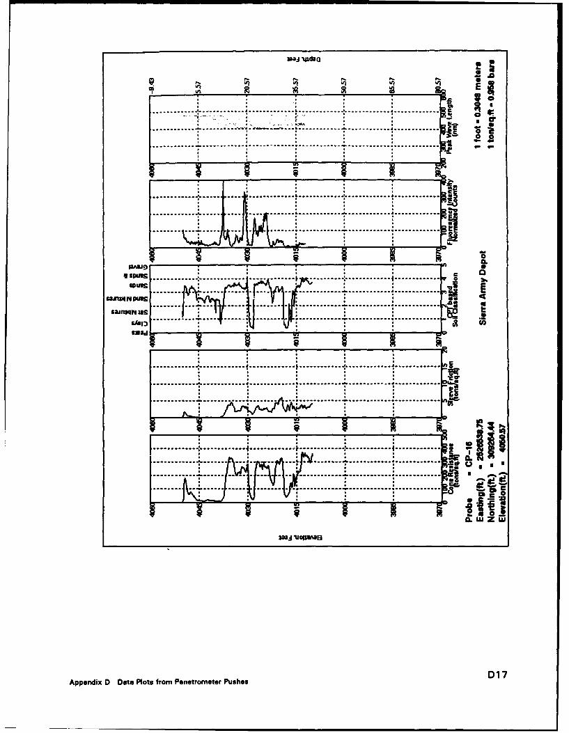
"I-- d I I IRAlao "pdaO
............ . ...... .. .. ........... L, -. -.
ci0 0
•US.................................................... ........... I............. : . ..... .. ......L........... .............. .............
............. L............,... ........ .. ........... . .......-..... -...--.... -....
..... -.... -----------
.............. . .... . . . . . . . . .. . .. . . .. . . . . .
SII4 IN
- -- -- -- -..............- .- , ,A- *
Ito
D17Appendix D Data Plots from Penetrometer Pushes
..........----------i, --------------------

, -- ..
- -t iI
. . . . --
'. cc
S............ :............ ...... ..... .. . . ... .,. .. . ..... =
S............. ............ .. . ......... ... ........ . ............. , .............. .......... .. . ............ . .
. .... ...- . .... . .. -. ........ . ... ........
----.--.-... -- . . ....... ... . ........ ........... ..........-... 0
* S •
"-* .... tin........... :_......_ _7. .. . .. ....... .............saiqnIOI PUR d
r4MI ..... . .
.. .. ....... ............. .
... .... . ..... . .... .. . ... .. .. ... .... . . .. . . .
....... ... . . .........
D0
.. . .. . . .. . . .. . . . . .. ... .. . . . . . . . . . c
c 0Z
D18 Appendix D Data Plots from Penetrometer Pushes
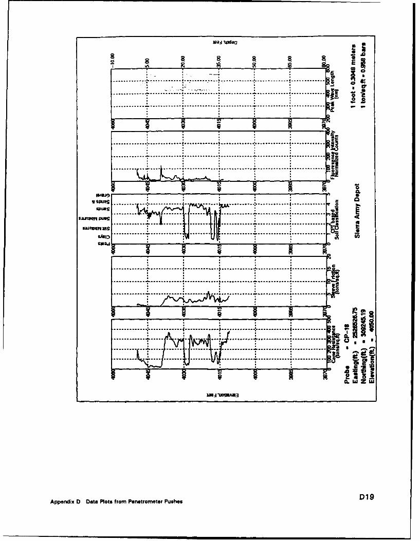
18a Uw~aa
7 C-
.. .. .. . -- -- - II .. ...... .. -- --- ---- - - -- - -- -- --
S........... .= , --. . .. -,--- ------, ----------. ......... . ............. .~0
S............. ,"-............ +,............. ,"............ ,--............ +,............. . I
............... + ............ i............. ............... -............ .............
':]. . . ; ... . . .. .. .... .. . . .. . .. . . .----- ... . . .. . . .. . .- ------ ------............ ............ .............
IRARJO C :;
SPURS
S.....~....... .. ............... .......u......" ............ .............~~~~. .......... . . .......... -------..! . .. . .. . • •
..... ......... .... ------- .........
S. .. .. .. .:-. . . . . ... ............. -------........ + ........... . ... . . . . o
* ....... . . ..-.- Uc
S...... + ...... :............. :1 ------------ -------- ------------- ............. 0•_r
............. + ............ ............ .+-:............ ÷ ............ "............. r. •'+
I 0
............. . ............. ,,........... , ............ ............... , ............. W..M "
wws....... W IA Il* ~ ..... ..o
S.......... i..... . :. .. . .. [..........------- i ............-- ............. • •s.......-u'................... .... ............ ............. L
... .... . . ..... ........ .............. ............ •.............-, o =ApenixD aePotfromPnermee Pses D I
-ME
-- - - - - - C.
..................... 0
-------- ca
Appendix D Data Plots from Penetrometer Pushes D19
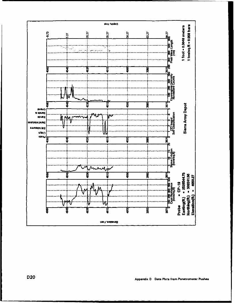
R N 'Nq 'N N
*.... .... *..... ................ ......... .. ....
CL
SPWCM AANSJd1 I.... . ... .... .... ........ ... ... ..-------
.a I,-~ rc n. "
V -*------ ----- ---- -------
. . . .. . . .L . . . . . . . . . . . . . . . . . . . ... . . . . . .. --- - - - - -
.. .. . . . . I -- - - --- -- -- - - - - - - - - -fi . . . . . . - - - - - -
............. ~ ~ ~ ~ ... .. .. . ..... .............. M L
. ... I ......... . ..... ....... ........
..... 4 ...... ..... . ....... --------........ C
D20 Appendix D Data Plots from Penetrometer Pushes

S.... ..... ..... . ... ................. ......................... . . .. . . •- l- 0 N
.......... .. .... ... . . .............. :
S... . . . ............. ;i ............. iL ............-':. . . .. .. " .............
0
S............. ............. :..............• ............ .:............. ............. •_
I'am
.°......... .... ° ... ....... ...... ............ ,.i.,.... .... ............ ....
.... . ......... .
. .......... .......... .. . ...... ......... I ..............9anl $pugs c 19ro
........... .. .. ............ .............
-~•31•. , *
sazw .. 43.........-- --.. --- ............ .............
.......... . .......................................
. . ...S.............. L..-...... ..... i.......... .......... .•- ": ............ .4...........
S.......;'',..... .... .... . .. ..ti tt ,• ....... 1.............. • , .
S............ .. .... . ... .. . . .. . "•....... ------ ------------- Mg i '•• •
,. ......... .. ........ ...... °,..°............
D21Appendix 0 Data Plots from Ponetrometer Pushes
• ,: •. um ai a aum il i N i • •i-1-5i

S............ -........ . .......... ... & ........ ............ .............00
S............ . .......................... "............ .- ............ ..............
i 2
............. ).L. ............ " ............ .............
CL
......................... . . .................. . ........... -----------.... 0
S*M j S-
....... *...° .... . .. . .. *°.................... M'
u*vr pu . S................................... "sa*n 5* 5 *
--------...----.-.-----------.---.----. .......... ............. . AD
=MCI
............ L............ ............. L............. L............ .............
............ ,. ............ ............. ............ ,............,..............
....... . ......... .... A .'U
........................................... .......... ...............................
.. .. .... . ......... .. ...... ..... .... .. .........c
I.0 us
D22 Appendix D Data Plots from Penetrometer Pushes

S. ................ -- --- -- ....... ...... , . .. ... .,. .......... ... , .........."...... . . .. ... .. .. . .. . ....... ... . . .. . .. . . .. .. . .. .
S......... . . .... ..... ,....... ..... ............ . ........... ...............
* *- * 6
-----....... c. .S.......i .... ...... ...... i............ ............. 0
espuvs**
..... r; / .......... . ... ............ L ............ i............. Migg
. ..... . ............ .........
...... ..... L .. .. .. . . . ........... .,'............ L . . . . . . ............. '"
* . .. 4.
... . . . . .......
................. ............ .--..-..
............. ." .... . ........ .-..... .
c c...... .:*.. : .. •• .... : .. .......a . .. .......,
z~z•3 oolwzw
D23Appendix D Data Plots from Penetrometer Pushes

Appendix EVerification Sample Information
Appendix E Verification Sample Information El

0 .... ... 2 ...0. . .. .4 6
- - NORMAL STR~ESS, 1VF
6 " TEST NO. 1
A 20 a*
WATER CONTENT, % .0 .0 .0
zVOID RATIO .761 .761 .761
SATURATION. X .0 .0 .0
DRY DENSITY. PCF 94.6 94.6 94.6
VOID RATIO AFTER CONSOL
FIFTY PERCENT OONSOL. MIN < I < 1 '1
-20 WATER CONTENT. .3 .3 .30 .1 .2 .3 .4 5VOID RATIO
HORIZ. DEFORMATION, IN. SATURATION, Xt
D- 0 EG NORMAL STRESS. TSF 1.00 2.00 3.00
MAXIMUM SHEAR STRESS. SF .56 1.56 2.36
TIME TO FAILURE. MIN 2 2 3
C- T/SF RATE OF STRAIN. IN/MIN .03339 .03339 .033339
ULTIMATE SHEAR STRESS. TSF .59 1.21 1.93
TYPE SPECIMEN COMPACTED 3.00 N. SOUARE .500 IN. THICK
CLASSIFICATION SLTY SAND (SM). BROWN
"LL PL PI GS 2.67 (EST
REMARKS; PROJECT SIERRA ARMY DEPOT
MOLDING CONDITIONS:
DRY DENSITY - 95 PCF BORING NO. OSA-SB-O1 SAMPLE 25,
WATER CONTENT - 0 X DEPTH/ELEV HOLL. STEM TECH. JH
LABORATORY USAE WES - SrF/GL DATE 23 NOV 93
DIRECT SHEAR TEST REPORT
E2 Appendix E Verification Sample Information
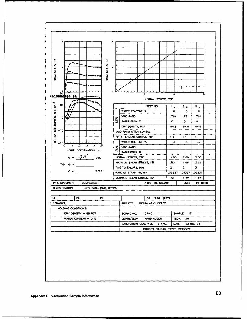
2 - 2-
20 0 .... ... .. ~ ......... * .......
202 4 6b15O9 *~*A -NORMAL STRESS. TSF
6 1o0 TEST NO. 1~ 2~ .3
a WATER CONTENT. X .0 .0 .0
0 VOI D RATIO .6 71 .6
2 SATURATION. % .0 .0 .0
- - -DRY DENSITY. PCF 94.6 94.6 94.6~-10 VOIDORAT10OAFrER CONSOL
-FlFrY PERCENT CNS0L. MIN .1 1 ~ 1
-20 .... ....~-~ WATER CONTENT. % .3 .3 .30 .1 .2 .3 . .OI O
HORIZ. DEFORMATION. IN . SATURATION,
cl - 35•'5 DEG NORMAL STRESS. TSF 1.00 2.00 3.00
TA b-MAXIMLIM SHEAR STRESS. TSF .80 1.66 2.352TIME TO FAIURE. MIN 2 2 3
C - ______T/SF RATE OF STRAIN, INIMIN .03337 .03337 .03337
ULTIMATE SHEAR STRESS. IS T .51 1.27 1.93
TYPE SPECIMEN COMPACTED 3.00 IN. .O .0 .0T
S OASSIFr tT.ON SILTY SAND (SM), BROWN
LL INP. PP CS 2.67 (EST)
REMARKS; PROJECT SIERRA ARMY DEPOT
MOLDING CONDOTTONS:
DRY DENSITY - 95 P BORING NO. CP-01 S
WATER CONTENT - 0 . DEPTH/EV HATND AUGER TECH. .JH
LOI.DFRA'•N N ABORATIORY USA WEI T L DAE _2NV9
MAXIMUM__HER_ _DIRECT SHEAR TEST REPORT
Appendix E Verification Sample Information E3
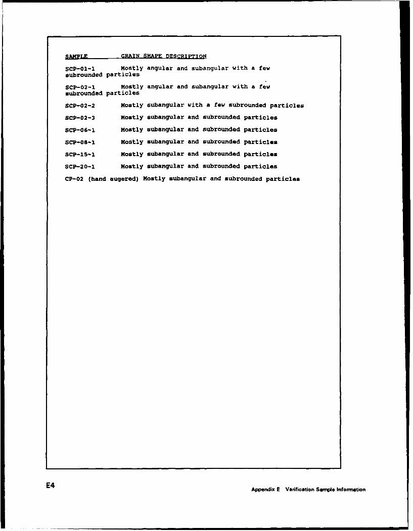
SAMPLE GRAIN SHAPE DESCRIPTION
SCP-01-1 Mostly angular and subangular with a fewsubrounded particles
SCP-02-1 Mostly angular and subangular with a fewsubrounded particles
SCP-02-2 Mostly subangular with a few subrounded particles
SCP-02-3 Mostly subangular and subrounded particles
SCP-06-1 Mostly subangular and subrounded particles
SCP-08-1 Mostly subangular and subrounded particles
SCP-15-1 Mostly subangular and subrounded particles
SCP-20-1 Mostly subangular and subrounded particles
CP-02 (hand augered) Mostly subangular and subrounded particles
E4 Appendix E Verification Sample Information
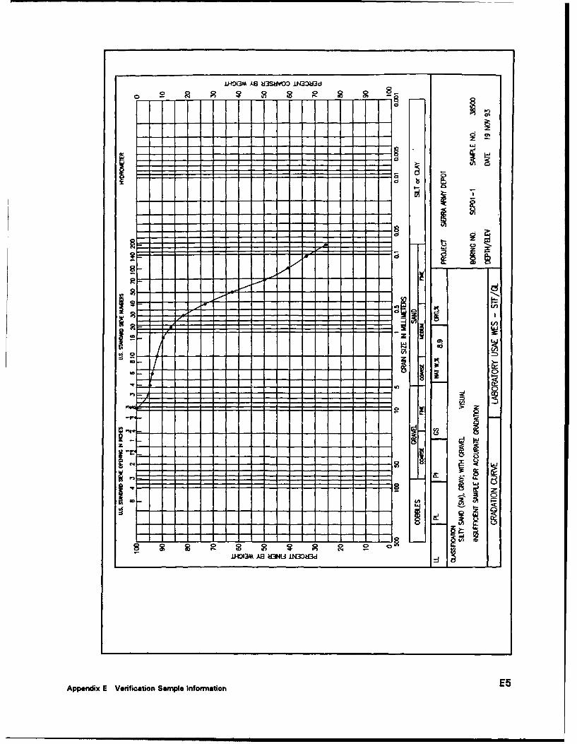
iHO13M AS 8A3S&N'OO JN3~3Gd
C2
I b
"p g-E-
I., C
r /o
- I
- -
Appendix E Verification Sample Information E5
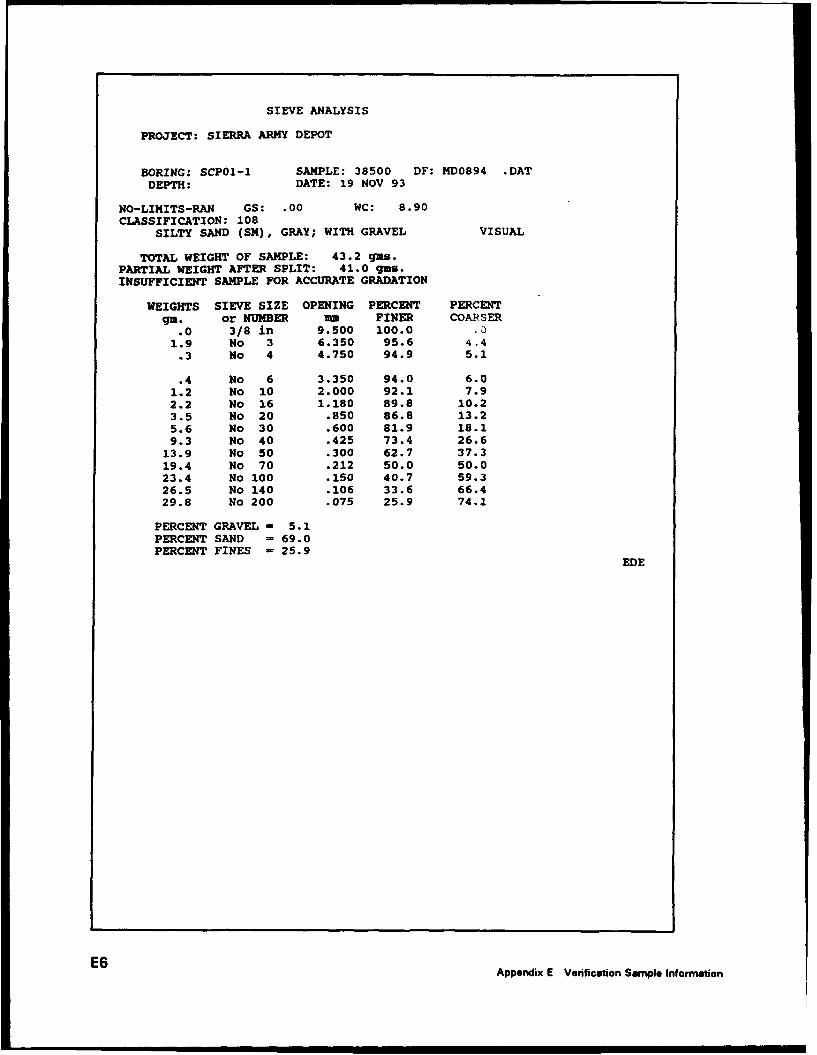
SIEVE ANALYSIS
PROJECT: SIERRA ARMY DEPOT
BORING: SCP01-1 SAMPLE: 38500 DF: MD0894 .DATDEPTH: DATE: 19 NOV 93
NO-LIMITS-RAN GS: .00 WC: 8.90CLASSIFICATION: 108
SILTY SAND (SM), GRAY; WITH GRAVEL VISUAL
TOTAL WEIGHT OF SAMPLE: 43.2 gns.PARTIAL WEIGHT AFTER SPLIT: 41.0 gms.INSUFFICIENT SAMPLE FOR ACCURATE GRADATION
WEIGHTS SIEVE SIZE OPENING PERCENT PERCENTg9. or NUMBER u-, FINER COARSER
.0 3/8 in 9.500 100.0 .31.9 No 3 6.350 95.6 4.4
.3 No 4 4.750 94.9 5.1
.4 No 6 3.350 94.0 6.01.2 No 10 2.000 92.1 7.92.2 No 16 1.180 89.8 10.23.5 No 20 .850 86.8 13.25.6 No 30 .600 81.9 18.19.3 No 40 .425 73.4 26.6
13.9 No 50 .300 62.7 37.319.4 No 70 .212 50.0 50.023.4 No 100 .150 40.7 59.326.5 No 140 .106 33.6 66.429.8 No 200 .075 25.9 74.1
PERCENT GRAVEL - 5.1PERCENT SAND = 69.0PERCENT FINES - 25.9
EDE
E6 Appendix E Verification Sample Information
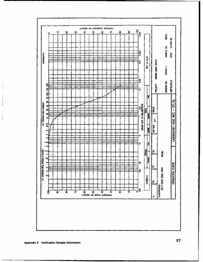
IJ-4OiM A 8 3SdWOO ±N33A:3d
-- P
--
L3 AAn
/d
If'
LK
- 0
Appendix E Verification Sample Information E7
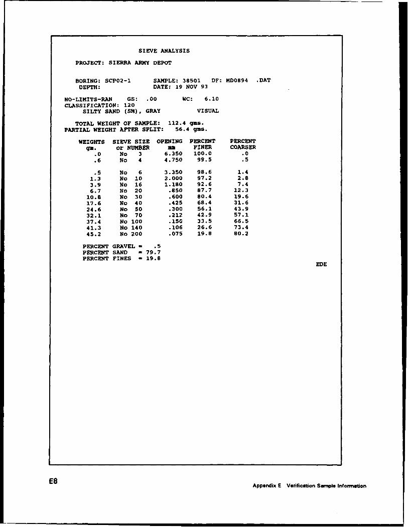
SIEVE ANALYSIS
PROJECT: SIERRA ARMY DEPOT
BORING: SCP02-1 SAMPLE: 38501 DF: MD0894 .DATDEPTH: DATE: 19 NOV 93
NO-LIMITS-RAN GS: .00 WC: 6.10CLASSIFICATION: 120
SILTY SAND (SM), GRAY VISUAL
TOTAL WEIGHT OF SAMPLE: 112.4 gas.PARTIAL WEIGHT AFTER SPLIT: 56.4 gus.
WEIGHTS SIEVE SIZE OPENING PERCENT PERCENTgm. or NUMBER Am FINER COARSER
.0 No 3 6.350 100.0 .0
.6 No 4 4.750 99.5 .5
.5 No 6 3.350 98.6 1.41.3 No 10 2.000 97.2 2.83.9 No 16 1.180 92.6 7.46.7 No 20 .850 87.7 12.3
10.8 No 30 .600 80.4 19.617.6 No 40 .425 68.4 31.624.6 No 50 .300 56.1 43.932.1 No 70 .212 42.9 57.137.4 No 100 .150 33.5 66.541.3 No 140 .106 26.6 73.445.2 No 200 .075 19.8 80.2
PERCENT GRAVEL = .5PERCENT SAND = 79.7PERCENT FINES = 19.8
EDE
E8 Appendix E Verification Sample Information

LH.OIM ASB WSW3SIo JN3N:13d
V,
a
I
-/- "- - It
-0
SICM
01
--flr
±HNI3M AB NI3NU 1)NMI3d
Appendix E Verification Sample Information E9
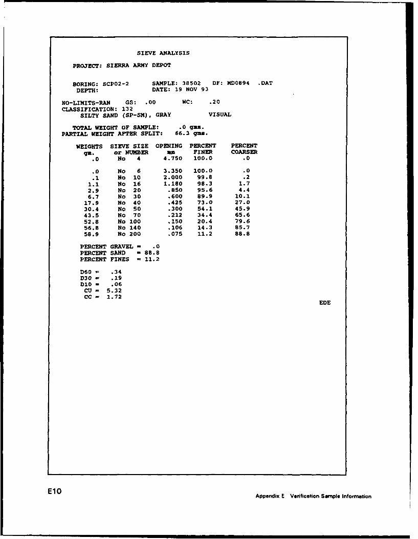
SIEVE ANALYSIS
PROJECT: SIERRA ARMY DEPOT
BORING: SCP02-2 SAMPLE: 38502 DF: MD0894 .DATDEPTH: DATE: 19 NOV 93
NO-LIMITS-RAN GS: .00 WC: .20CLASSIFICATION: 132
SILTY SAND (SP-SM), GRAY VISUAL
TOTAL WEIGHT OF SAMPLE: .0 gns.PARTIAL WEIGHT AFTER SPLIT: 66.3 gas.
WEIGHTS SIEVE SIZE OPENING PERCENT PERCENTqz. or NUMBER MI FINER COARSER
.0 No 4 4.750 100.0 .0
.0 No 6 3.350 100.0 .0
.1 No 10 2.000 99.8 .21.1 No 16 1.180 98.3 1.72.9 No 20 .850 95.6 4.46.7 No 30 .600 89.9 10.1
17.9 No 40 .425 73.0 27.030.4 No 50 .300 54.1 45.943.5 No 70 .212 34.4 65.652.8 No 100 .150 20.4 79.656.8 No 140 .106 14.3 85.758.9 No 200 .075 11.2 88.8
PERCENT GRAVEL - .0PERCENT SAND = 88.8PERCENT FINES - 11.2
D60 - .34D30 = .19010 - .06
CU = 5.32CC - 1.72
EDE
E 10 Appendix E Verification Sample Information

H1.3M AS ýJ SOO S• JJ.J333d
05
to-N
d n
z -
C>
- " -"- C •
Appendix E Verification Sample Information Ell
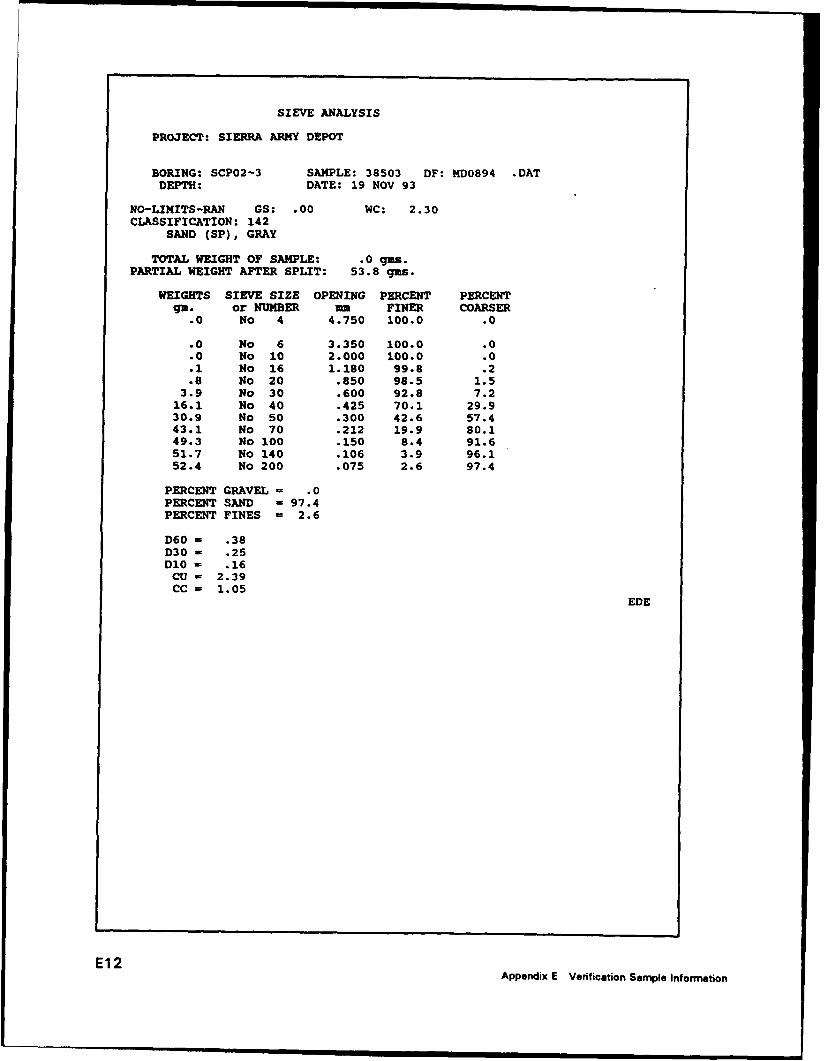
SIEVE ANALYSIS
PROJECT: SIERRA ARMY DEPOT
BORING: SCP02-3 SAMPLE: 38503 DF: MD0894 .DATDEPTH: DATE: 19 NOV 93
NO-LIMITS-RAN GS: .00 WC: 2.30CLASSIFICATION: 142
SAND (SP), GRAY
TOTAL WEIGHT OF SAMPLE: .0 gms.PARTIAL WEIGHT AFTER SPLIT: 53.8 gus.
WEIGHTS SIEVE SIZE OPENING PERCENT PERCENTga. or NUMBER MR FINER COARSER
.0 No 4 4.750 100.0 .0
.0 No 6 3.350 100.0 .0
.0 No 10 2.000 100.0 .0
.1 No 16 1.180 99.8 .2.8 No 20 .850 98.5 1.5
3.9 No 30 .600 92.8 7.216.1 No 40 .425 70.1 29.930.9 No 50 .300 42.6 57.443.1 No 70 .212 19.9 80.149.3 No 100 .150 8.4 91.651.7 No 140 .106 3.9 96.152.4 No 200 .075 2.6 97.4
PERCENT GRAVEL - .0PERCENT SAND - 97.4PERCENT FINES = 2.6
D60 = .38D30 - .25D10 = .16
CU - 2.39CC = 1.05
EDE
E12 Appendix E Verification Sample Information
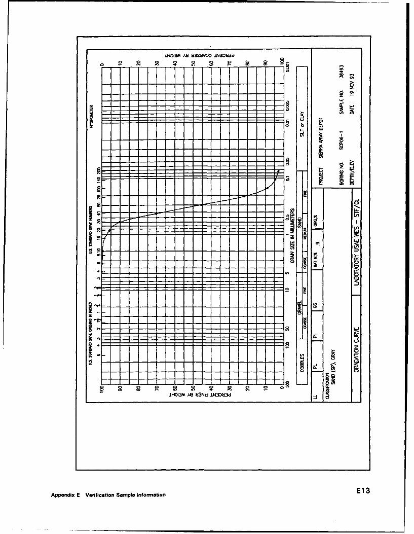
,I-013M AS M3SbVO3 IN30ýd
LJ
d
01
Paa
-: z:1 •1zz
MHOIM A9 kI3NU IN3:?:4i
Appendix E Verification Sample Information E 13
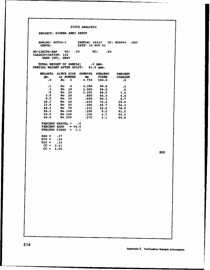
SIEVE ANALYSIS
PROJECT: SIERRA ARMY DEPOT
BORING: SCP06-1 SAMPLE: 38493 DF: MD0894 .DATDEPTH: DATE: 19 NOV 93
NO-LIMITS-RAN GS: .00 WC: .90CLASSIFICATION: 152
SAND (SP), GRAY
TOTAL WEIGHT OF SAMPLE: .0 gus.PARTIAL WEIGHT AFTER SPLIT: 61.9 gus.
WEIGHTS SIEVE SIZE OPENING PERCENT PERCENTgm. or NUMBER au FINER COARSER
.0 No 4 4.750 100.0 .0
.1 No 6 3.350 99.8 .2
.3 No 10 2.000 99.5 .5
.9 No 16 1.180 98.5 1.52.5 No 20 .850 96.0 4.06.0 No 30 .600 90.3 9.7
18.3 No 40 .425 70.4 29.633.6 No 50 .300 45.7 54.348.3 No 70 .212 22.0 78.056.3 No 100 .150 9.0 91.059.0 No 140 .106 4.7 95.360.0 No 200 .075 3.1 96.9
PERCENT GRAVEL = .0PERCENT SAND = 96.9PERCENT FINES = 3.1
D60 = .37D30 = .24D10 = .15
CU = 2.41CC = 1.02
EDE
E14Appendix E Verification Sample Information

LU-tOGM AS &I3SUVO3 iN33Md
- 0
--- - -
aL
-J ,
-V
_- S •~-e
iAi r3M Ae HI3NU iNin l r nd
Appendix E Verification Sample Information E15

SIEVE ANALYSIS
PROJECT: SIERRA ARMY DEPOT
BORING: SCP08-1 SAMPLE: 38496 DF: MD0894 .DAT
DEPTH: DATE: 19 NOV 93
NO-LIMITS-RAN GS: .00 WC: 12.00CLASSIFICATION: 162
SILTY SAND (SM), BROWN VISUAL
TOTAL WEIGHT OF SAMPLE: .0 gas.PARTIAL WEIGHT AFTER SPLIT: 52.3 gas.
WEIGHTS SIEVE SIZE OPENING PERCENT PERCENT
gm. or NUMBER Am FINER COARSER.0 No 4 4.750 100.0 .0
.1 No 6 3.350 99.8 .2
.6 No 10 2.000 98.9 1.11.5 No 16 1.180 97.1 2.93.2 No 20 .850 93.9 6.15.9 No 30 .600 88.7 11.3
12.2 No 40 .425 76.7 23.319.7 No 50 .300 62.3 37.727.1 No 70 .212 48.2 51.832.2 No 100 .150 38.4 61.635.6 No 140 .106 31.9 68.138.7 No 200 .075 26.0 74.0
PERCENT GRAVEL = .0PERCENT SAND = 74.0PERCENT FINES = 26.0
EDE
E1 6 Appendix E Verification Sample Information
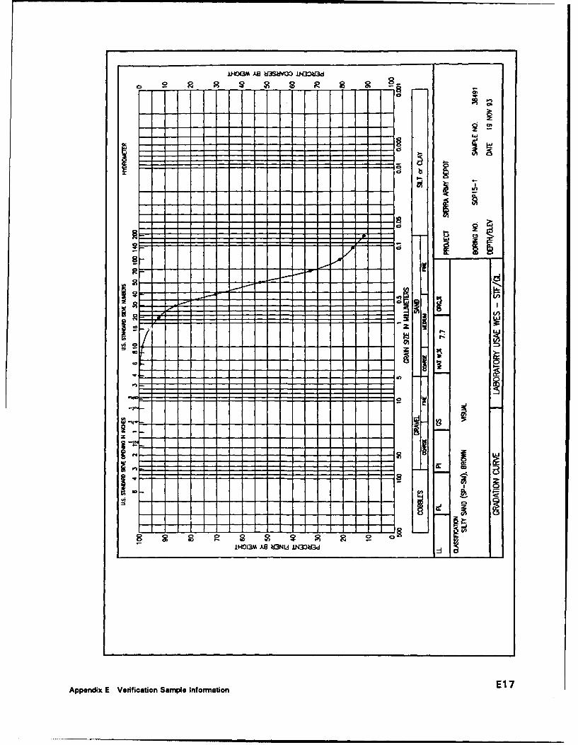
..OGm ASE W3SWW itQOGd
a-
fI
so X
MII
O 1HO13M A,, HNU4 iN3O3?33
Appendix E Verification Sample Information E1 7
S .. ........ . . .. -- - -- m m .m- - - - -Iml m
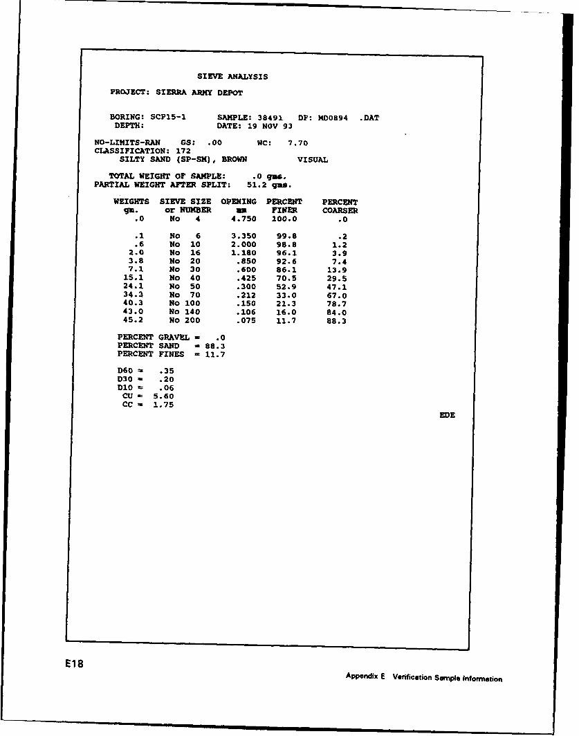
SIEVE ANALYSIS
PROJECT: SIERRA ARMY DEPOT
BORING: SCP15-1 SAMPLE: 38491 DF: MD0894 .DATDEPTH: DATE: 19 NOV 93
NO-LIMITS-RAN GS: .00 WC: 7.70CLASSIFICATION: 172
SILTY SAND (SP-SM), BROWN VISUAL
TOTAL WEIGHT OF SAMPLE: .0 gus.PARTIAL WEIGHT AFTER SPLIT: 51.2 gus.
WEIGHTS SIEVE SIZE OPENING PERCENT PERCENTgia. or NUMBER am FINER COARSER
.0 No 4 4.750 100.0 .0
.1 No 6 3.350 99.8 .2
.6 No 10 2.000 98.8 1.22.0 No 16 1.180 96.1 3.93.8 No 20 .850 92.6 7.47.1 No 30 .600 86.1 13.9
15.1 No 40 .425 70.5 29.524.1 No 50 .300 52.9 47.134.3 No 70 .212 33.0 67.040.3 No 100 .150 21.3 78.743.0 No 140 .106 16.0 84.045.2 No 200 .075 11.7 88.3
PERCENT GRAVEL - .0PERCENT SAND = 88.3PERCENT FINES = 11.7
D60 - .35D30 - .20D10 - .06
CU , 5.60CC - 1.75
EDE
E18Appendix E Verification Semple Information

".11
B03~M A93S aNU JJ433t3d
I
z z
-ig
I 0
E19Appendix E Verification Sample Information

SIEVE ANALYSIS
PROJECT: SIERRA ARMY DEPOT
BORING: SCP20-1 SAMPLE: 38494 DF: MD0894 .DATDEPTH: DATE: 19 NOV 93
NO-LIMITS-RAN GS: .00 WC: 1.80CLASSIFICATION: 182
SILTY SAND (SP-SM), GRAY VISUAL
TOTAL WEIGHT OF SAMPLE: .0 gas.PARTIAL WEIGHT AFTER SPLIT: 54.2 gas.
WEIGHTS SIEVE SIZE OPENING PERCENT PERCENTga. or NUMBER Mu FINER COARSER
.0 No 4 4.750 100.0 .0
.0 No 6 3.350 100.0 .0
.1 No 10 2.000 99.8 .21.0 No 16 1.180 98.2 1.82.6 No 20 .850 95.2 4.85.6 No 30 .600 89.7 10.3
14.6 No 40 .425 73.1 26.924.0 No 50 .300 55.7 44.335.8 No 70 .212 33.9 66.147.0 No 100 .150 13.3 86.749.8 No 140 .106 8.1 91.950.9 No 200 .075 6.1 93.9
PERCENT GRAVEL - .0PERCENT SAND = 93.9PERCENT FINES - 6.1
D60 - .33D30 - .20D10 - .12
CU - 2.71CC - .99
EDE
E20 Appendix E Verification Sample Information
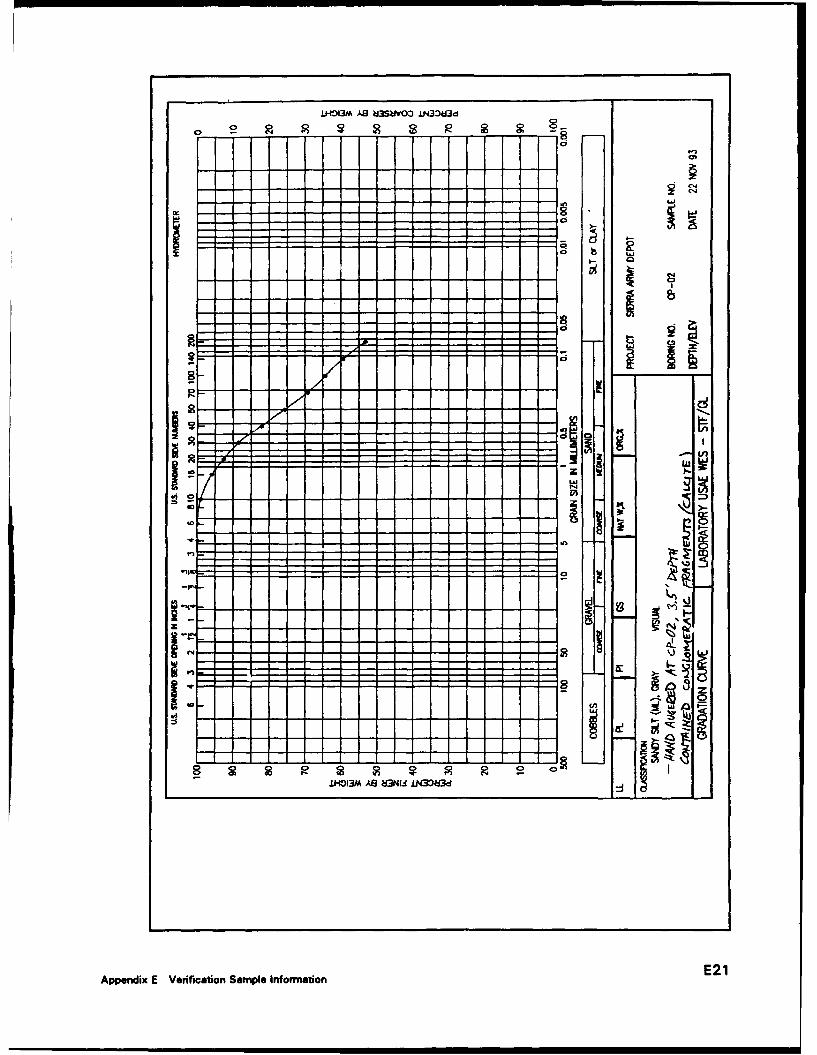
LHOG3M As2 Uj3Sevao 1NG3ý3d
-- . -J -
/ ttC-.-
*0 A
AV_.
0iiIT:-------- ll°~'
Appenix----------------ple-nfom-tin-E2

SIEVE ANALYSIS
PROJECT: SIERRA ARMY DEPOT
BORING: CP-02 SAMPLE: DF: MD0894A .DATDEPTH: DATE: 22 NOV 93
NO-LIMITS-RAN GS: .00 WC: .00CLASSIFICATION: 122
SANDY SILT (ML), GRAY VISUAL
TOTAL WEIGHT OF SAMPLE: .0 gus.PARTIAL WEIGHT AFTER SPLIT: 55.2 gas.
WFPIGHTS SIEVE SIZE OPENING PERCENT PERCENTgm. or NUMBER n FINER COARSER
.0 No 4 4.750 100.0 .0
.0 No 6 3.350 100.0 .0
.5 No 10 2.000 99.1 .92.2 No 16 1.180 96.0 4.04.0 No 20 .850 92.8 7.26.3 No 30 .600 88.6 11.49.8 No 40 .425 82.2 17.8
13.4 No 50 .300 75.7 24.316.9 No 70 .212 69.4 30.619.7 No 100 .150 64.3 35.722.4 No 140 .106 59.4 40.625.8 No 200 .075 53.3 46.7
PERCENT GRAVEL - .0PERCENT SAND = 46.7PERCENT FINES = 53.3
EDE
E22 Appendix E Verification Sample Information
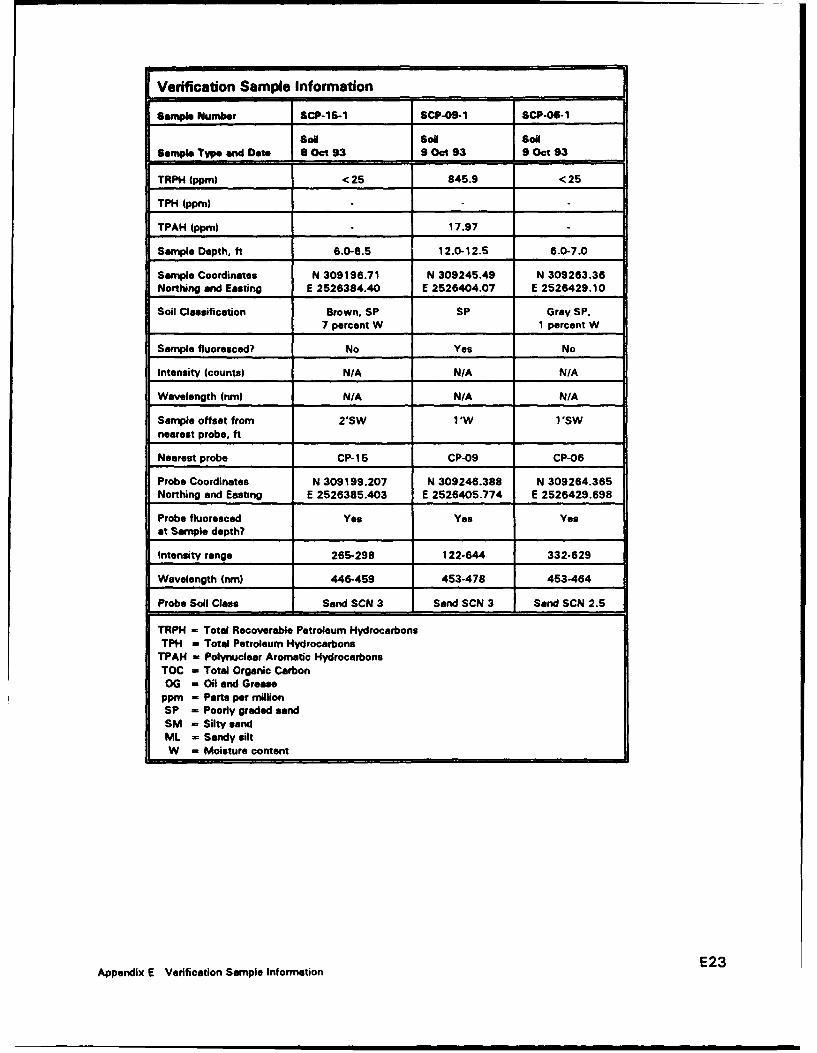
Verification Sample Information
Sample Numb.r SCP-15-1 SCP-09-1 SCP-06-1
SONl Sol SoilSample Type and Date 8 Oct 93 9 Oct 93 9 Oct 93
TRPH (ppm) < 25 845.9 <25
TPH (ppm) _ _
TPAH (ppm) 17.97
Sample Depth, ft 6.0-6.5 12.0-12.5 6.0-7.0
Sample Coordinates N 309196.71 N 309245.49 N 309263.36Northing and Easting E 2526384.40 E 2526404.07 E 2526429.10
Soil Classification Brown, SP SP Gray SP.7 percent W 1 percent W
Sample fluoresced? No Yes No
Intensity (counts) N/A N/A N/A
Wavelength (nm) N/A N/A N/A
Sample offset from 2'SW 1 'W 1 "SWnearest probe, ft
Nearest probe CP-15 CP-09 CP-06
Probe Coordinates N 309199.207 N 309246.388 N 309264.365Northing and Easting E 2526385.403 E 2526405.774 E 2526429.698
Probe fluoresced Yes Yes Yesat Sample depth?
Intensity range 265-298 122-644 332-629
Wavelength (rn) 446-459 453-478 453-464
Probe Soil Class Sand SCN 3 Sand SCN 3 Sand SCN 2.5
TRPH , Total Recoverable Petroleum HydrocarbonsTPH - Total Petroleum HydrocarbonsTPAH , Polynuclear Aromatic HydrocarbonsTOC , Total Organic CarbonOG - Oil and Grease
pprn Parts per millionSP - Poorly graded sandSM , Silty sandML = Sandy siltW , Moisture content
E23Appendix E Verification Sample Information

Verification Sample Information
Sample Number SCP-14-3 SCP-17-1 SCP-17-2
Sod Sol sodSample Typo and Date 8 Oct 93 8 Oct 93 8 Oct 93
TRPH (ppm) 11445 7228 1784
TPH (ppm)
TPAH (ppm) 28.6 3.29 1.25
Sample Depth, ft 19.0-19.5 20.5-21.0 23.0-23.5
Sample Coordinates N 309239.25 N 309257.35 N 309257.35Northing and Easting E 2526515.41 E 2526535.25 E 2526535.25
Soil Classification Tan SP Tan SP Brown SP
Sample fluoresced? Yes Yes Yes
Intensity (counts) N/A N/A N/A
Wavelength (nm) N/A N/A N/A
Sample offset from 1 'SW 2'S 2'Snearest probe, ft
Nearest probe CP-14 CP-17 CP-17
Probe Coordinates N 309240.055 N 309258.357 N 309258.357
Northing end Easting E 2526516.410 E 2526534.252 E 2526534.252
Probe fluoresced Yes Yes Yesat Sample depth?
Intensity range 83-241 447-579 357-664
Wavelength (nm) 452-473 399-409 394-411
Probe Soil Class Sand SCN 3 Sand SCN 2.5 Sand SCN 3.5
TRPH - Total Recoverable Petroleum HydrocarbonsTPH - Total Petroleum Hydrocarbons
TPAH - Poiynuclear Aromatic HydrocarbonsTOC - Total Organic CarbonOG - Oil and Grease
ppm - Parts per millionSP - Poorly graded sandSM - Silty sandML - Sandy siltW = Moisture content
E24 Appendix E Verification Sample Information

Verification Sample Information
Sample Number 8CP-02-3 SCP-02-4 SCP-17-3
Sample Type and Date 10 Oct 93 10 Oct 93 10 Oct 93
TRPH (ppm) <25 <25 5817
TPH (ppm) __ ___
TPAH (ppm) 3.03
Sample Depth, ft 7.75-8.5 8.5-10.0 20.0-20.5
Sample Coordinates N 309431.45 N 309431.45 N 309257.35Northing and Easting E 2526632.01 E 2526632.01 E 2526536.25
Soil Classification Gray SP. Gray SP Gray SP2 percent Water
Sample fluoresced? No No Yes
Intensity (counts) N/A N/A N/A
Wavelength (nm) N/A N/A N/A
Sample offset from 1'S 1'S 2'SEnearest probe, ft
Nearest probe CP-02 CP-02 CP-17
Probe Coordinates N 309431.956 N 309431.956 N 309258.357Northing and Easting E 2526632.016 E 2526632.016 E 2526534.252
Probe fluoresced Yes Yes Yesat Sample depth?
Iniensity range 38-331 28-340 270-549
Wavelength (nm) 413-475 398-480 398-409
Probe Soil Class Sand SCN 3 Sand SCN 3 Sand SCN 3.5
=TRPH - Total Recoverable Petroleum HydrocarbonsTPH = Total Petroleum Hydrocarbons
TPAH = Polynuolear Aromatic Hydrocarbons
TOC = Total Organic CarbonOG = Oil and Grease
ppm = Parts per millionSP - Poorly graded sandSM - Silty sandML = Sandy siltW - Moisture content
E25Appendix E Verification Sample Information

Verification Sample Information
Sample Number SCP-12-1 SCP.14-1 SCP-14-2
Soil SoN solSample Typ and Date 8 Oct 93 8 Oct 93 8 Oct 93
TRPH (ppm) <25 203.2 22151
TPH (ppm) -
TPAH (ppm) 0 62.9
Sample Depth, ft 6.5-7.5 13.0-14.5 18.0
Sample Coordinates N 309229.47 N 309239.25 N 309239.25Northing end Easting E 2526475.23 E 2526515.41 E 2526515.41
Soil Classification Brown SP-SM Brown SP Brown SP
Sample fluoresced? No Yes Yes
Intensity (counts) N/A N/A N/A
Wavelength (nm) N/A N/A N/A
Sample offset from 2'W 1 1SW 1'SWnearest probe, ft
Nearest probe CP-12 CP-14 CP-14
Probe Coordinates N 309230.067 N 309240.055 N 309240.055
Northing and Easting E 2526477.727 E 2526516.410 E 2526516.410
Probe fluoresced Yes Yes Yes
at Sample depth?
Intensity range 112-207 46-393 132-241
Wavelength (nm) 445-461 399-476 398-477
Probe Soil Class Sand SCN 2.5 Sand SCN 3.5 Sand SCN 3.5
TRPH - Total Recoverable Petroleum HydrocarbonsTPH - Total Petroleum HydrocarbonsTPAH = Polynuclear Aromatic HydrocarbonsTOC = Total Organic Carbon
OG = Oil and Greaseppm - Parts per millionSP - Poorly graded sandSM - Silty sand
ML = Sandy siltW = Moisture content
E26 Appendix E Verification Sample Information

Verification Sample Information
Sample Number SCP-O1-1 SCP-02-1 SCP-02-2
Soil Soil $oilSample Type and Date 10 Oct 93 10 Oct 93 10 Oct 93
TRPH (ppm) <25 <25 <25
TPH (ppm) _ _ _ _
TPAH (ppm)
Sample Depth. ft 4.0-5.0 3.0-4.0 7.0-7.75
Sample Coordinates N 309437.83 N 309431.45 N 309431.45Northing and Easting E 2526504.12 E 2526632.01 E 2526632.01
Soil Classification Gray SM, Gray SM, Gray SP,9 percent W 6 percent W 0.2 percent W
Sample fluoresced? No No No
Intensity (counts) N/A N/A N/A
Wavelength (nm) N/A N/A N/A
Sample offset from 1'S 1'S 1'S
nearest probe, ft
Nearest probe CP-01 CP-02 CP-02
Probe Coordinates N 309438.336 N 309431.956 N 309431.956Northing and Easting E 2526503.622 E 2526632.016 E 2526632.016
Probe fluoresced Yes Yes Yesat Sample depth?
Intensity range 234-414 197-243 40.139
Wavelength (nm) 457-467 450-457 422-452
Probe Soil Class Silt SCN 2 Silt SCN 2 Sand SCN 3
TRPH - Total Recoverable Petroleum HydrocarbonsTPH , Total Petroleum Hydrocarbons
TPAH , Polynuclear Aromatic HydrocarbonsTOC ,=Total Organic Carbon06 Oil and Grease
ppm ,- Parts per millionSP = Poorly graded sand
SM , Silty sandML Sandy siltW T Moisture content
E27Appendix E Verification Sample Information

Verification Sample Information
Samole Number 8CP-08-2 SCP-06-1 SCP-05-2
Soil Soa SoaSample Type and Date 9 Oct 93 9 Oct 93 9 Oct 93
TRPH (ppm) <25 <25 <25
TPH (ppm) -
TPAH (ppm)
Sample Depth. ft 7.5-8.0 7.5-8.0 8.5-9.0
Sample Coordinates N 309240.84 N 309361.92 N 309361.92Northing and Easting E 2526597.86 E 2526573.43 E 2526573.43
Soil Classification Gray SP-SM Gray SM-ML Brown SM
Sample fluoresced? No No No
Intensity (counts) N/A N/A N/A
Wavelength (nm) N/A N/A N/A
Sample offset from I'SE 2'W 2'Wnearest probe, ft
Nearest probe CP-08 CP-05 CP-05
Probe Coordinates N 309242.344 N 309362.917 N 309362.917Northing and Easting E 2526597.862 E 2526574.429 E 2526574.429
Probe fluoresced Yes Yes Yesat Sample depth? j
Intensity range 151-305 215-343 246-495
Wavelength (nm) 447-456 453-458 453-458
Probe Soil Class Silt SCN 3 Silty Sand SCN 2 Sand SCN 2.5
TRPH - Total Recoverable Petroleum HydrocarbonsTPH - Total Petroleum Hydrocarbons
TPAH = Polynuclear Aromatic HydrocarbonsTOC - Total Organic CarbonOG - Oil end Grease
ppm - Parts per millionSP - Poorly graded sendSM - Silty sendML - Sandy siltW - Moisture content
E28 Appendix E Verification Sample Information

Verification Sample Information
Sanmple Number SCP-20-1 SCP-19-1 SCP-0S-1
Soil Soil 6o11Sample Type and Date 9 Oct 93 9 Oct 93 9 Oct 93
TRPH (ppm) <25 <25 <25
TPH (ppm) _ _ _
TPAH (ppm)
Sample Depth, ft 7.0-7.5 3.5-4.5 2.5-3.0
Sample Coordinates N 309214.99 N 309242.06 N 309240.84Northing and Easting E 2526529.77 E 2526544.26 E 2526597.86
Soil Classification Gray SP. Ten SP Brown SM,2 percent W 12 percent W
Sample fluoresced? No No Nn
Intensity (counts) N/A N/A N/A
Wavelength (nm) N/A N/A N/A
Sample offset from 1 'W 0.6'N 1 'SEnearest probe, ft
Nearest probe CP-20 CP-19 CP-08
Probe Coordinates N 309216.495 N 309241.555 N 309242.344Northing and Easting E 2526530.272 E 2526544.756 E 2526597.862
Probe fluoresced Yes Yes Yesat Sample depth?
Intensity range 95-171 99-209 258-338
Wavelength (nm) 451-485 457-488 452-455
Probe Soil Class Sand SCN 3 Sand SCN 3 Send SCN 3
TRPH = Total Recoverable Petroleum HydrocarbonsTPH , Total Petroleum HydrocarbonsTPAH , Polynuclear Aromatic HydrocarbonsTOC - Total Organic Carbon
OG , Oil and Greaseppm - Parts per millionSP = Poorly graded sandSM = Silty sandML = Sandy siltW , Moisture content
E29Appendix E Verification Sample Information
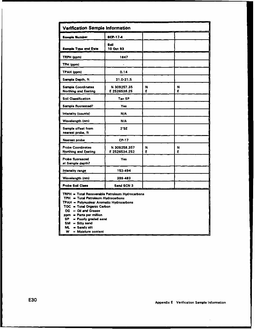
Verification Sample Information
Sample Number SCP- 17-4
So__Sample Type and Date 10 Oct 93
TRPH (ppm) 1847
"TPH (ppm) _
TPAH (ppm) 0.14
Sample Depth, ft 21.0-21.5
Sample Coordinates N 309257.35 N NNorthing and Easting E 2526536.25 E E
Soil Classification Tan SP
Sample fluoresced? Yes
Intensity (counts) N/A
Wavelength (nrm) NIA
Sample offset from 2'SEnearest probe, ft
Nearest probe CP- 17
Probe Coordinates N 309258.357 N NNorthing and Easting E 2526534.252 E E
Probe fluoresced Yesat Sample depth?
Intensity range 153-494
Wavelength (nm) 399-483
Probe Soil Class Sand SCN 3
TRPH ,= Total Recoverable Petroleum HydrocarbonsTPI4 , Total Petroleum Hydrocarbons
TPAH ,= Polynuolear Aromatic HydrocarbonsTOC = Total Organic Carbon
OG = Oil and Greaseppm ,- Parts per millionSP ,, Poorly graded sandSM ,= Silty sandML ,= Sandy siltW = Moisture content
E30 Appendix E Verification Sample Information
- Ti i i "-
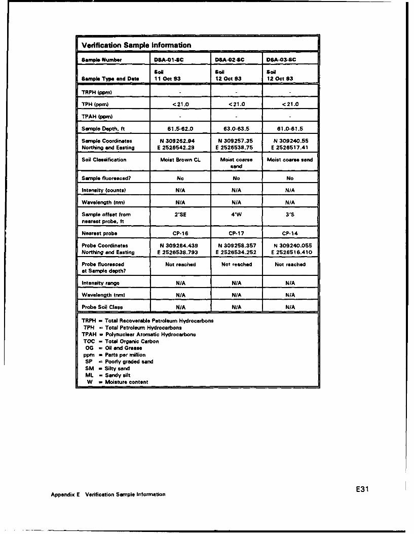
Verification Sample Information
Sample Number DSA-01-aC DSA-02-4C DSA-03-SC
SOil Sail SoilSample Type and Date 11 Oct 93 12 Oct 93 12 Oct 93
TRPH (ppm)
TPH (ppm) <21.0 <21.0 <21.0
TPAH (ppm) _ _
Sample Depth, ft 61.5-62.0 63.0-63.5 61.0-61.5
Sample Coordinates N 309262.94 N 309257.35 N 309240.55Northing and Easting E 2526542.29 E 2526538.75 E 2526517.41
Soil Classification Moist Brown CL Moist coarse Moist coarse sandsand
Sample fluoresced? No No No
Intensity (counts) N/A N/A N/A
Wavelength (nm) N/A N/A N/A
Sample offset from 2'SE 4'W 3'Snearest probe, ft
Nearest probe CP-16 CP-17 CP-14
Probe Coordinates N 309264.439 N 309258.357 N 309240.055
Northing and Easting E 2526538.793 E 2526534.252 E 2526516.410
Probe fluoresced Not reached Not reached Not reachedat Sample depth?
Intensity range N/A N/A N/A
Wavelength (nm) N/A N/A N/A
Probe Soil Class N/A N/A N/A
TRPH - Total Recoverable Petroleum HydrocarbonsTPH - Total Petroleum Hydrocarbons
TPAH = Polynuclear Aromatic HydrocarbonsTOC - Total Organic CarbonOG = Oil and Grease
ppm - Parts per millionSP = Poorly graded sandSM = Silty sandML - Sandy siltW - Moisture content
E31Appendix E Verification Sample Information
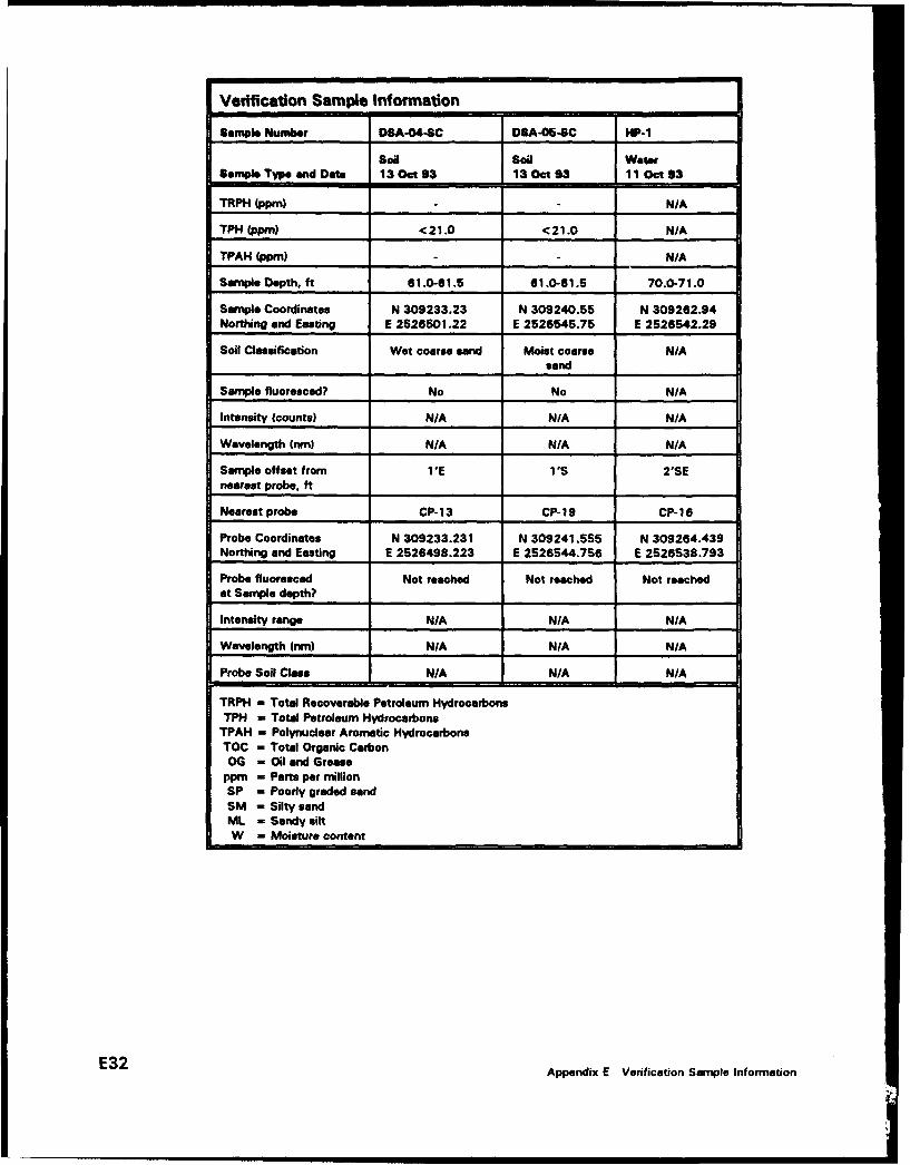
Verification Sample Information
Sample Number DSA-04-SC DSA-06-SC HP-1
SoNl Soil WaterSample Type and Date 13 Oct 93 13 Oct 93 11 Oct 93
TRPH (ppm) - - N/A
TPH (ppm) <21.0 <21.0 N/A
TPAH (ppm) - N/A
Sample Depth, ft 61.0-61.5 61.0-61.5 70.0-71.0
Sample Coordinates N 309233.23 N 309240.55 N 309262.94Northing and Easting E 2526501.22 E 2526545.75 E 2526542.29
Soil Classification Wet coarse sand Moist coarse N/Asand
Sample fluoresced? No No N/A
Intensity (counts) N/A N/A NIA
Wavelength (Om) N/A N/A N/A
Sample offset from 1 'E 1'S 2"SEnearest probe. ft
Nearest probe CP-13 CP- 19 CP- 16
Probe Coordinates N 309233.231 N 309241.555 N 309264.439Northing and Easting E 2526498.223 E 2526544.756 E 2526538.793
Probe fluoresced Not reached Not reached Not reachedat Sample depth?
Intensity range N/A N/A N/A
Wavelength (am) N/A N/A N/A
Probe Soil Class N/A N/A N/ATRPH I Taev
TRPH - Total Recoverable Petroleum HydrocarbonsTPH -= Total Petroleum Hydrocarbons
TPAH - Polynuclear Aromatic HydrocarbonsTOC - Total Organic Carbon00 - Oil and Grease
ppm = Parts per millionSP - Poorly graded sandSM = Silty sandML = Sandy siltW = Moisture content
E32 Appendix E Verification Sample Information
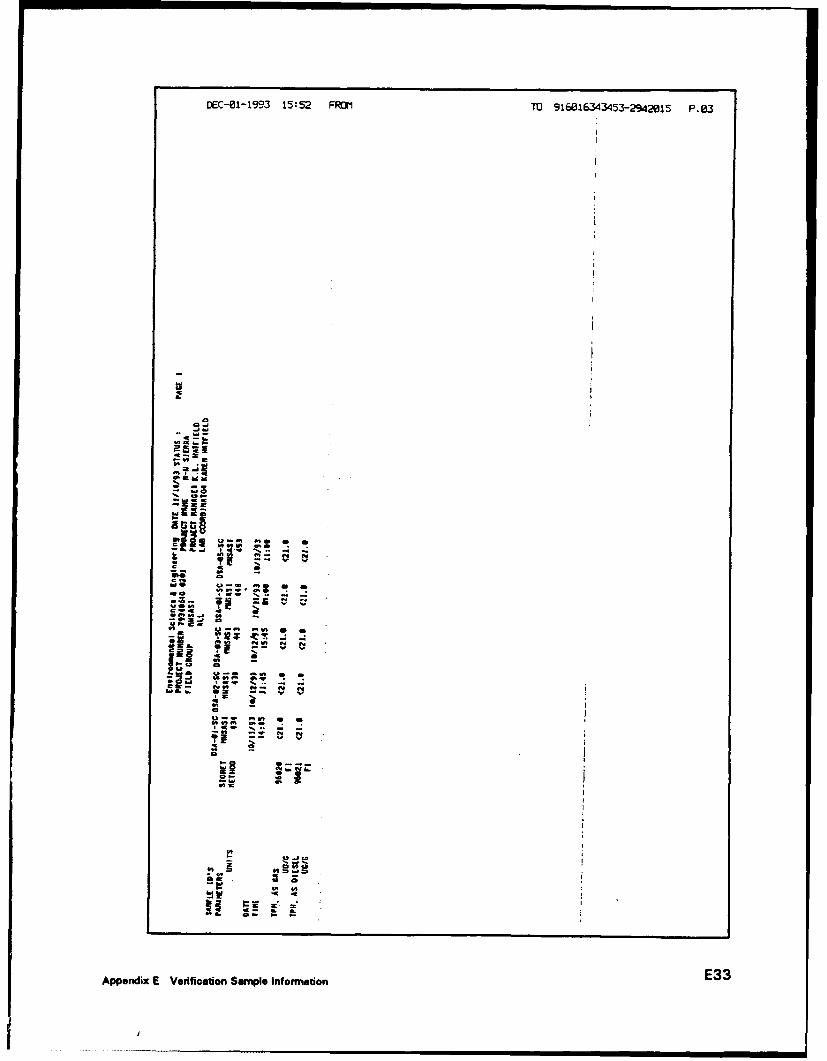
DEC-e1-1993 15:52 FROM TO 916e16343453-2934•:g5 P. e3
•5
=Ia
4I--'
-, .4 " g
Appendix Veiiat nSnl nfrto 3

Dmc-01-1is3 15:53 FROM TO 96016343453-2942015 P.04
ANa -. I a
, a,• .. V
=M I
"i"~~c cis.II i ti•ii .,, 6"s 1
- Q
A
4 0T
S..
-V* -,
rill
W 4
TOTAL P.0
E34 Appendix E Verification Samlple Infor...twon

Form Approvedi
REPORT DOCUMENTATION PAGE OMB No 0704-0188
Putbhc reporting burden for this coiieClton of information -% estimated to Olerage ; hour o r reine ,,nse c auding the time for reviewing instrilu irS toia icnig e-scting data sources
athefin and maintaining the data needed. and (omp eiting and ief-ewmng the ot lectom of 'formatiot Send comments regarding ths burden estimatc or an, Other asoea of this
?61 t9 On of Informat;on mcluding suggestions tot reducing th14 curden to Wathnrton mesoauarter$ Services. Direcict ate for rltormation Oerations and Recorts, 12 1 jefferson
es H~ghwof. Suite 1•204. Adhngton. VA 22202-4302. and to the Offce of Management and Budget Paperwork Reducton Prolect (0704-0188)) as•n•gton. DC 20S03
f. AGENCY USE ONLY (Leave blank) 2. REPORT DATE 3. REPORT TYPE AND DATES COVERED
I February 1994 Final report
4. TITLE AND SUBTITLE S. FUNDING NUMBERS
Site Characterization and Analysis Penetrometer System (SCAPS)Field Investigations at the Sierra Army Depot, California
6. AUTHOR(S)
Landris T. Lee, Jr., William M Davis, Ricky A. Goodson,Jeff F. Powell, and Bryan A. Register
7. PERFORMING ORGANIZATION NAME(S) AND ADDRESS(ES) 8. PERFORMING ORGANIZATIONREPORT NUMBER
U.S. Army Engineer Waterways Experiment StationGeotechnical Laboratory, Environmental Laboratory Technical ReportInstrumentation Services Division GL-94-43909 Halls Ferry Road, Vicksburg, MS 39180-6199
9. SPONSORING/ MONITORING AGENCY NAME(S) AND ADDRESS(ES) 10. SPONSORING /MONITORING
AGENCY REPORT NUMBER
U.S. Army Environmental CenterAberdeen Proving Ground, MD 21010-5401
11. SUPPLEMENTARY NOTES
12a. DISTRIBUTION/AVAILABILITY STATEMENT 12b. DISTRIBUTION CODE
Approved for public release; distribution is unlimited.
13. ABSTRACT (Maximum 200 words)
The WES Site Characterization and Analysis Penetrometer System (SCAPS) investigated a diesel spill site at theSierra Army Depot near Herlong, California. The truck-mounted laser-induced fluorometer packaged with theconventional cone penetrometer was utilized for this mission. Soil and groundwater verification sampling for onsiteand laboratory analyses was also conducted. Extensive comparisons of verification sampling data were performed,and POL contamination was detected in some of those samples and in situ.
14. SUBJECT TERMS 15. NUMBER OF PAGES
Cone penetrometer Soil stratigraphy 165Laser-induced fluorometer Verification sampling 16. PRICE CODEPOL contamination
17. SECURITY CLASSIFICATION 18. SECURITY CLASSIFICATION 19. SECURITY CLASSIFICATION 20. LIMITATION OF ABSTRACTOF REPORT OF THIS PAGE OF ABSTRACT
UNCLASSIFIED UNCLASSIFIED I INSN 7540-01-280-5500 Standard Form 298 (Rev 2-89)
Prescribed b, ANSi Sitd Z39-1B
298-102