US Age and Sex Composition

7/27/2019 US Age and Sex Composition

http://slidepdf.com/reader/full/us-age-and-sex-composition 1/16

U.S. Department o Commerce Economics and Statistics Administration U.S. CENSUS BUREAU

Age and Sex Composition: 20102010 Census Briefs

By

Lindsay M. Howden

and

Julie A. Meyer

C2010BR-03

Issued May 2011

INTRODUCTION

Focusing on a population’s

age and sex composition is

one o the most basic ways to

understand population change

over time. Since Census 2000,

the population has continued

to grow older, with many

states reaching a median age

over 40 years. At the same

time, increases in the num-

ber o men at older ages are

apparent. Understanding a population’s

age and sex composition yields insights

into changing phenomena and highlights

uture social and economic challenges.

This report describes the age and sex

composition o the United States in 2010.

It is part o a series that provides an

overview o the population and housing

data collected rom the 2010 Census.

It highlights analysis o age and sex at

the national level, as well as or regions,

states, and counties and or places with

populations o 100,000 or more. A com-

parison with Census 2000 data is also

provided, showing the changes in age and

sex composition that have taken place

over the last 10 years.

This report also provides inormation

about how age and sex data were col-

lected in the 2010 Census. The data or

this report are based on the 2010 Census Summary File 1, which is among the

irst 2010 Census data products to be

released.1

SEX AND AGE QUESTIONS

Data on the sex and age composition o

the United States and your community are

derived rom the 2010 Census questions

on sex, age, and date o birth (Figure 1).

The sex question remains unchanged rom

the previous census. Inormation on the

sex o individuals is one o the ew items

obtained in the original 1790 Census and

in every census since.

As with sex, inormation on age has been

collected since 1790. The 2010 Census

age data were derived rom a two-part

question. The irst part asked or the age

o the person, and the second part asked

or the date o birth. The question is

1 The 2010 Census Summary File 1 (SF1) con-tains data on age, sex, race, Hispanic origin, groupquarters, relationship, tenure, and households at avariety o geographic levels down to the block level.For a detailed schedule o 2010 Census products andrelease dates, visit <www.census.gov/population/www/cen2010/glance/index.html >.

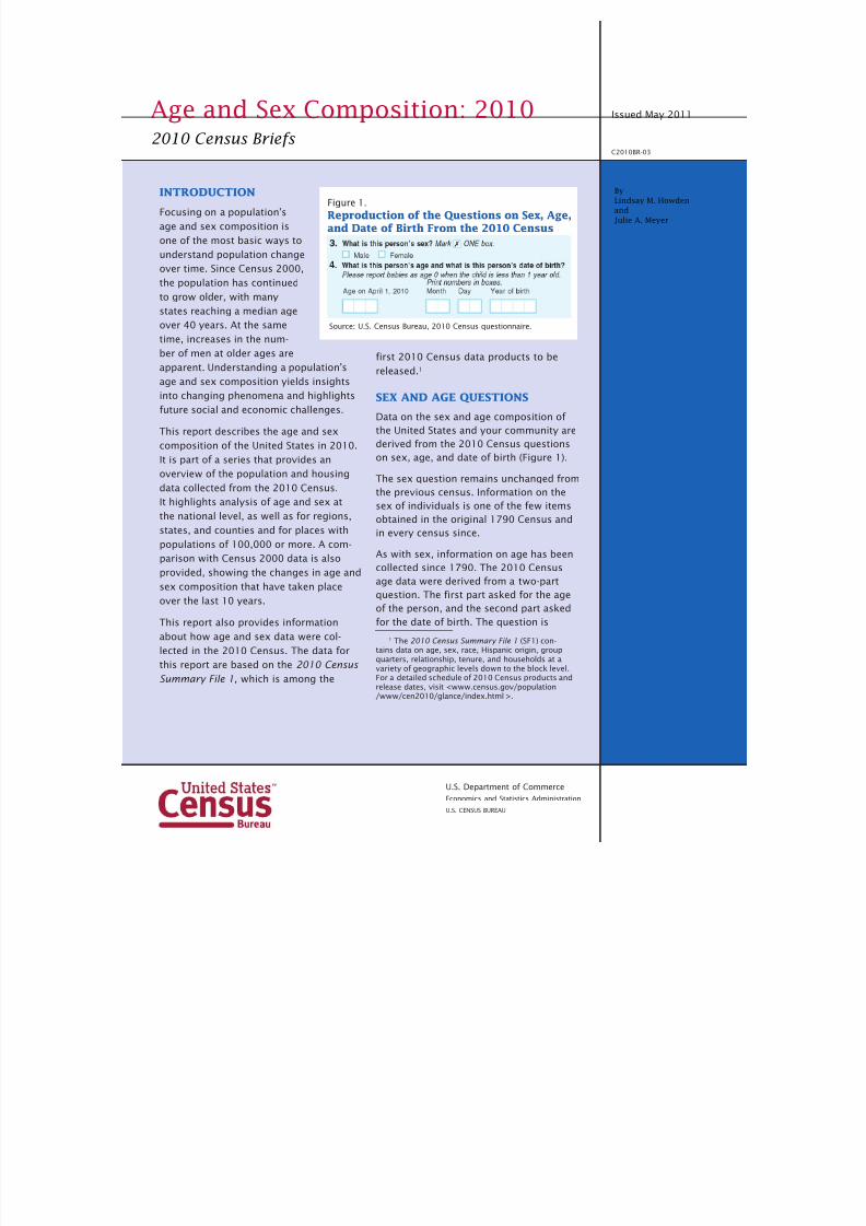
Figure 1.

Reproduction of the Questions on Sex, Age,and Date of Birth From the 2010 Census

Source: U.S. Census Bureau, 2010 Census questionnaire.

http://www.census.gov/population/www/cen2010/glance/index.html






2 U.S. Census Bureau

designed in two parts in order to

maximize both the accuracy and

the number o people responding

to this item. The age question itsel

is unchanged since Census 2000,

however, an instruction was added

to guide respondents to report

the ages o babies as 0 years old

i they were less than 1 year old.

In previous censuses, research-

ers ound that respondents otenreported their babies’ ages in terms

o days, weeks, or months, rather

than in terms o years. This instruc-

tion was added to reduce reporting

problems or babies.

AGE AND SEX COMPOSITION

According to the 2010 Census, the

population o the United States on

April 1, 2010, was 308.7 million

people, representing a 9.7 per-

cent increase in population since2000, when the population was

281.4 million (Table 1). Growth

was slower than the 13.2 percent

increase experienced during the

previous decade, but similar to the

growth between 1980 and 1990

(9.8 percent). O the 2010 Census

population, 157.0 million were

emale (50.8 percent) while 151.8

million were male (49.2 percent).

Between 2000 and 2010, the male

population grew at a slightly aster

rate (9.9 percent) than the emale

population (9.5 percent).

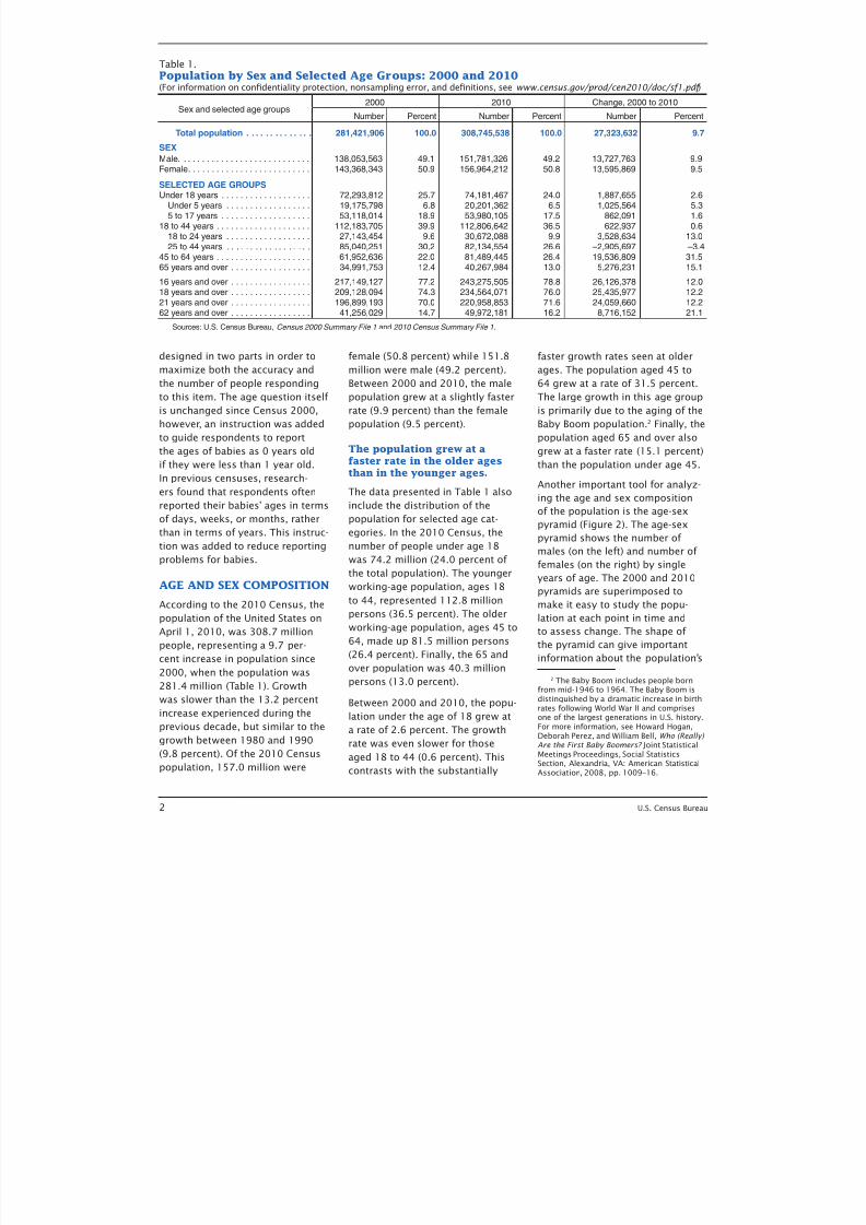
The population grew at afaster rate in the older agesthan in the younger ages.

The data presented in Table 1 alsoinclude the distribution o the

population or selected age cat-

egories. In the 2010 Census, the

number o people under age 18

was 74.2 million (24.0 percent o

the total population). The younger

working-age population, ages 18

to 44, represented 112.8 million

persons (36.5 percent). The older

working-age population, ages 45 to

64, made up 81.5 million persons

(26.4 percent). Finally, the 65 and

over population was 40.3 million

persons (13.0 percent).

Between 2000 and 2010, the popu-

lation under the age o 18 grew at

a rate o 2.6 percent. The growth

rate was even slower or those

aged 18 to 44 (0.6 percent). This

contrasts with the substantially

aster growth rates seen at older

ages. The population aged 45 to

64 grew at a rate o 31.5 percent.

The large growth in this age group

is primarily due to the aging o the

Baby Boom population.2 Finally, the

population aged 65 and over also

grew at a aster rate (15.1 percent)

than the population under age 45.

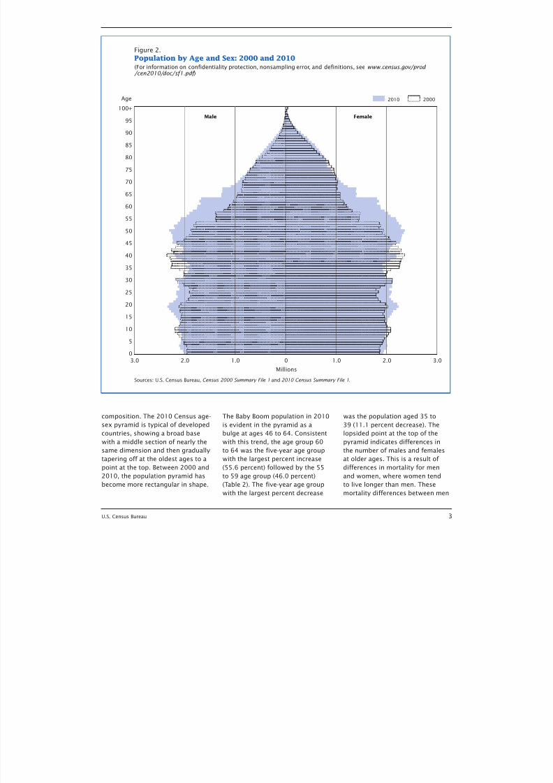
Another important tool or analyz-

ing the age and sex compositiono the population is the age-sex

pyramid (Figure 2). The age-sex

pyramid shows the number o

males (on the let) and number o

emales (on the right) by single

years o age. The 2000 and 2010

pyramids are superimposed to

make it easy to study the popu-

lation at each point in time and

to assess change. The shape o

the pyramid can give important

inormation about the population’s2 The Baby Boom includes people born

rom mid-1946 to 1964. The Baby Boom isdistinguished by a dramatic increase in birthrates ollowing World War II and comprisesone o the largest generations in U.S. history.For more inormation, see Howard Hogan,Deborah Perez, and William Bell, Who (Really) Are the First Baby Boomers? Joint StatisticalMeetings Proceedings, Social StatisticsSection, Alexandria, VA: American StatisticalAssociation, 2008, pp. 1009–16.

Table 1.Population by Sex and Selected Age Groups: 2000 and 2010(For inormation on confdentiality protection, nonsampling error, and defnitions, see www.census.gov/prod/cen2010/doc/sf1.pdf )

Sex and selected age groups2000 2010 Change, 2000 to 2010

Number Percent Number Percent Number Percent

Total population 281,421,906 1000 308,745,538 1000 27,323,632 97

SEX

Male 138,053,563 491 151,781,326 492 13,727,763 99Female 143,368,343 509 156,964,212 508 13,595,869 95

SELECTED AGE GROUPSUnder 18 years 72,293,812 257 74,181,467 240 1,887,655 26

Under 5 years 19,175,798 68 20,201,362 65 1,025,564 535 to 17 years 53,118,014 189 53,980,105 175 862,091 16

18 to 44 years 112,183,705 399 112,806,642 365 622,937 0618 to 24 years 27,143,454 96 30,672,088 99 3,528,634 13025 to 44 years 85,040,251 302 82,134,554 266 –2,905,697 –34

45 to 64 years 61,952,636 220 81,489,445 264 19,536,809 31565 years and over 34,991,753 124 40,267,984 130 5,276,231 151

16 years and over 217,149,127 772 243,275,505 788 26,126,378 12018 years and over 209,128,094 743 234,564,071 760 25,435,977 12221 years and over 196,899,193 700 220,958,853 716 24,059,660 12262 years and over 41,256,029 147 49,972,181 162 8,716,152 211

Sources: US Census Bureau, Census 2000 Summary File 1 and 2010 Census Summary File 1



U.S. Census Bureau 3

composition. The 2010 Census age-

sex pyramid is typical o developedcountries, showing a broad base

with a middle section o nearly the

same dimension and then gradually

tapering o at the oldest ages to a

point at the top. Between 2000 and

2010, the population pyramid has

become more rectangular in shape.

The Baby Boom population in 2010

is evident in the pyramid as abulge at ages 46 to 64. Consistent

with this trend, the age group 60

to 64 was the ive-year age group

with the largest percent increase

(55.6 percent) ollowed by the 55

to 59 age group (46.0 percent)

(Table 2). The ive-year age group

with the largest percent decrease

was the population aged 35 to

39 (11.1 percent decrease). Thelopsided point at the top o the

pyramid indicates dierences in

the number o males and emales

at older ages. This is a result o

dierences in mortality or men

and women, where women tend

to live longer than men. These

mortality dierences between men

Figure 2.

Population by Age and Sex: 2000 and 2010

2010

(For information on confidentiality protection, nonsampling error, and definitions, see www.census.gov/prod /cen2010/doc/sf1.pdf )

Male Female

Age 2000

Sources: U.S. Census Bureau, Census 2000 Summary File 1 and 2010 Census Summary File 1.

Millions

0 1.0 2.0 3.03.0 2.0 1.0

0

5

10

15

20

25

30

35

40

45

50

55

60

65

70

75

80

85

90

95

100+




and women also impact another

important indicator o population

composition, the sex ratio.

Faster growth in the male

population led to increasedsex ratios.

The sex ratio is a common mea-

sure used to describe the balance

between males and emales in the

population. It is deined as the

number o males per 100 emales.

A sex ratio o exactly 100 would

indicate an equal number o males

and emales, with a sex ratio under

100 indicating a greater number o

emales. The sex ratio at birth in

the United States has been around

105 males or every 100 emales,

however, since mortality at every

age is generally higher or males,

the sex ratio naturally declines

with age. This tendency progresses

through ages 85 and above where

there are considerably more surviv-

ing women. These trends result in

more males at younger ages and

more emales at older ages. Sex

ratios can vary rom these pat-

terns or many reasons such as the

impact o international or domes-

tic migration on a population or

eatures o the geographic location

(or example, the existence o col-

lege student housing or military

acilities).

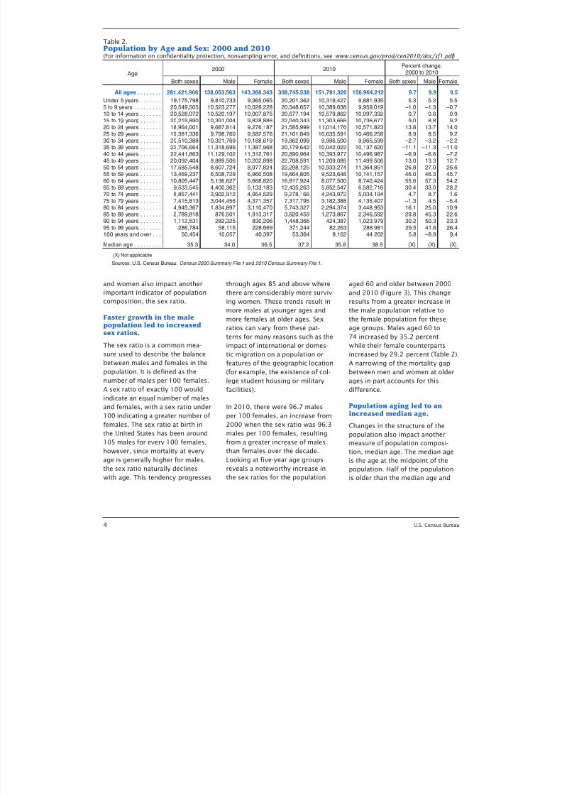
In 2010, there were 96.7 males

per 100 emales, an increase rom

2000 when the sex ratio was 96.3

males per 100 emales, resulting

rom a greater increase o males

than emales over the decade.

Looking at ive-year age groups

reveals a noteworthy increase in

the sex ratios or the population

aged 60 and older between 2000

and 2010 (Figure 3). This change

results rom a greater increase in

the male population relative to

the emale population or these

age groups. Males aged 60 to

74 increased by 35.2 percent

while their emale counterparts

increased by 29.2 percent (Table 2).

A narrowing o the mortality gap

between men and women at older

ages in part accounts or this

dierence.

Population aging led to anincreased median age.

Changes in the structure o the

population also impact another

measure o population composi-

tion, median age. The median age

is the age at the midpoint o the

population. Hal o the population

is older than the median age and

Table 2.Population by Age and Sex: 2000 and 2010(For inormation on confdentiality protection, nonsampling error, and defnitions, see www.census.gov/prod/cen2010/doc/sf1.pdf )

Age2000 2010

Percent change,2000 to 2010

Both sexes Male Female Both sexes Male Female Both sexes Male Female

All ages 281,421,906 138,053,563 143,368,343 308,745,538 151,781,326 156,964,212 97 99 95

Under 5 years

5 to 9 years 10 to 14 years 15 to 19 years 20 to 24 years 25 to 29 years 30 to 34 years 35 to 39 years 40 to 44 years 45 to 49 years 50 to 54 years 55 to 59 years 60 to 64 years 65 to 69 years 70 to 74 years 75 to 79 years 80 to 84 years

85 to 89 years 90 to 94 years 95 to 99 years 100 years and over

19,175,798 9,810,733 9,365,065 20,201,362 10,319,427 9,881,935 53 52 55

20,549,505 10,523,277 10,026,228 20,348,657 10,389,638 9,959,019 –10 –13 –0720,528,072 10,520,197 10,007,875 20,677,194 10,579,862 10,097,332 07 06 0920,219,890 10,391,004 9,828,886 22,040,343 11,303,666 10,736,677 90 88 9218,964,001 9,687,814 9,276,187 21,585,999 11,014,176 10,571,823 138 137 14019,381,336 9,798,760 9,582,576 21,101,849 10,635,591 10,466,258 89 85 9220,510,388 10,321,769 10,188,619 19,962,099 9,996,500 9,965,599 –27 –32 –2222,706,664 11,318,696 11,387,968 20,179,642 10,042,022 10,137,620 –111 –113 –11022,441,863 11,129,102 11,312,761 20,890,964 10,393,977 10,496,987 –69 –66 –7220,092,404 9,889,506 10,202,898 22,708,591 11,209,085 11,499,506 130 133 12717,585,548 8,607,724 8,977,824 22,298,125 10,933,274 11,364,851 268 270 26613,469,237 6,508,729 6,960,508 19,664,805 9,523,648 10,141,157 460 463 45710,805,447 5,136,627 5,668,820 16,817,924 8,077,500 8,740,424 556 573 5429,533,545 4,400,362 5,133,183 12,435,263 5,852,547 6,582,716 304 330 2828,857,441 3,902,912 4,954,529 9,278,166 4,243,972 5,034,194 47 87 167,415,813 3,044,456 4,371,357 7,317,795 3,182,388 4,135,407 –13 45 –544,945,367 1,834,897 3,110,470 5,743,327 2,294,374 3,448,953 161 250 109

2,789,818 876,501 1,913,317 3,620,459 1,273,867 2,346,592 298 453 2261,112,531 282,325 830,206 1,448,366 424,387 1,023,979 302 503 233

286,784 58,115 228,669 371,244 82,263 288,981 295 416 26450,454 10,057 40,397 53,364 9,162 44,202 58 –89 94

Median age 353 340 365 372 358 385 (X) (X) (X)

(X) Not applicable

Sources: US Census Bureau, Census 2000 Summary File 1 and 2010 Census Summary File 1.




hal o the population is younger.

The median age is oten used to

describe the “age” o a popula-

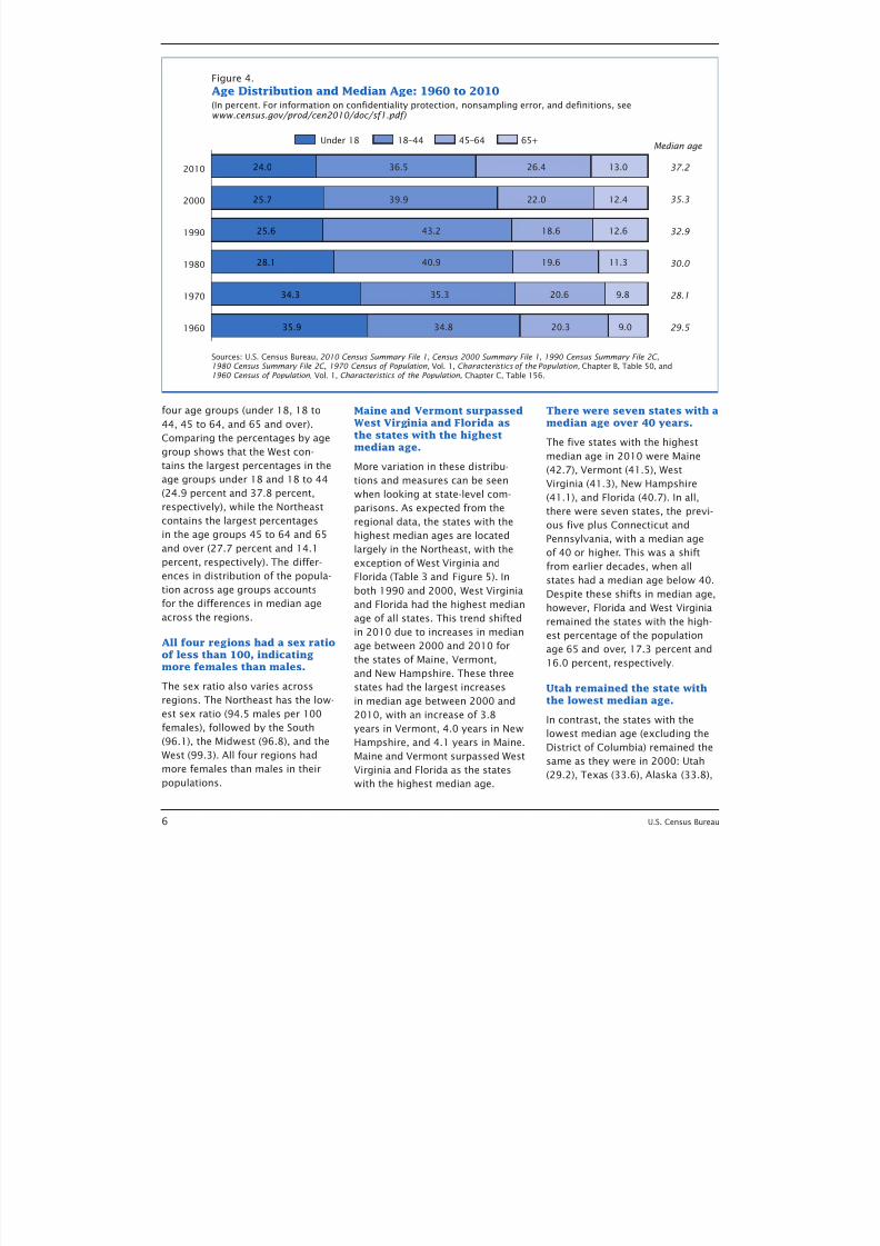
tion. In 2010, the median age

increased to a new high o 37.2

years, rom 35.3 years in 2000,

with the proportion o the popula-

tion at the older ages increasing

similarly (Figure 4). This indicates

that the U.S. population is aging.

Globally, the median age o the

United States is higher than coun-

tries that are less developed, but

younger than most more-developed

countries.3 The 1.9 year increase3 More-developed regions include all

regions o Europe, plus Northern America,Australia/New Zealand, and Japan. Less-developed regions include all regionso Arica, Asia (excluding Japan), LatinAmerica, and the Caribbean, plus Melanesia,Micronesia, and Polynesia. For moreinormation, see Population Division o theDepartment o Economic and Social Aairso the United Nations Secretariat, World Population Prospects: The 2008 Revision,<http://esa.un.org/unpp>.

between 2000 and 2010 was more

modest than the 2.4 year increase

in median age between 1990 and

2000. The aging o the Baby Boom

population into older age groups

is contributing to the increase in

median age. In the United States,

other contributors include stable

birth rates and improving mortality.

DIFFERENCES IN AGE ANDSEX BY GEOGRAPHY

A major strength o census data

is its detail available at low levels

o geography that can highlight

variation in age and sex across the

United States. This section com-

pares basic age and sex distribu-

tions and selected measures among

the geographies within regions,

states, and counties as well as

places with 100,000 or more

population.

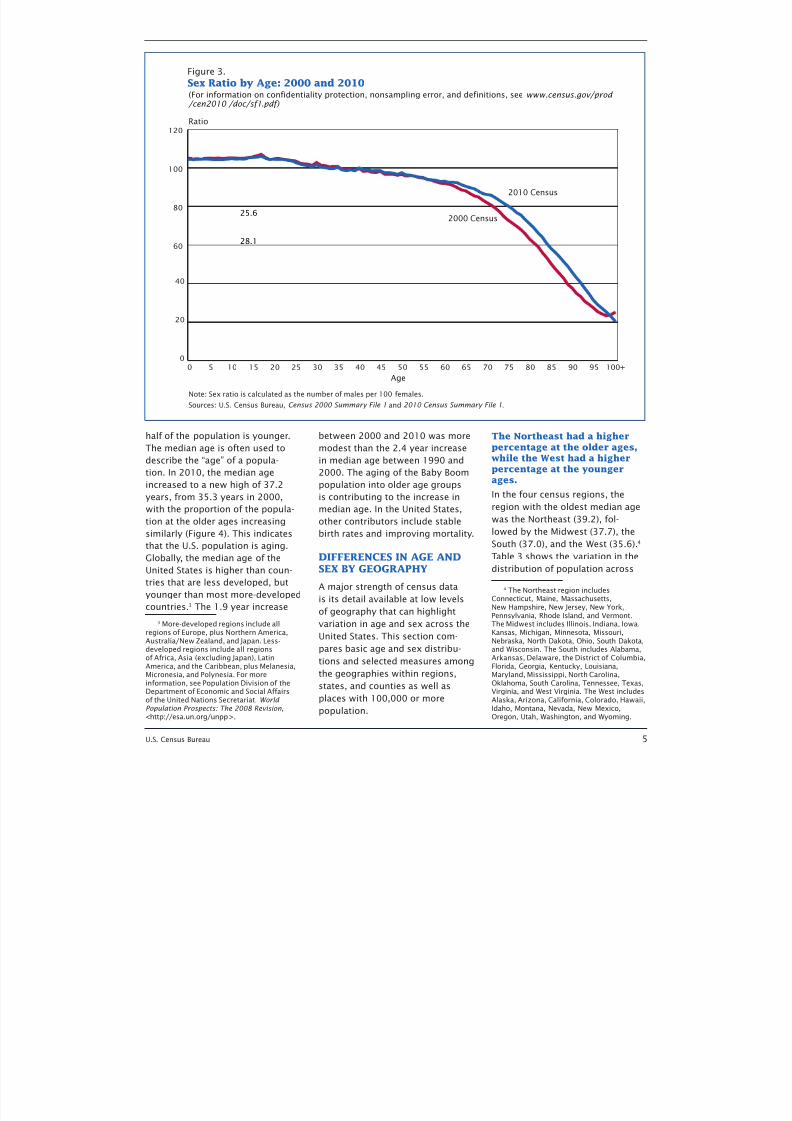
The Northeast had a higherpercentage at the older ages,

while the West had a higherpercentage at the youngerages.

In the our census regions, the

region with the oldest median age

was the Northeast (39.2), ol-

lowed by the Midwest (37.7), the

South (37.0), and the West (35.6).4

Table 3 shows the variation in the

distribution o population across

4 The Northeast region includesConnecticut, Maine, Massachusetts,

New Hampshire, New Jersey, New York,Pennsylvania, Rhode Island, and Vermont.The Midwest includes Illinois, Indiana, Iowa,Kansas, Michigan, Minnesota, Missouri,Nebraska, North Dakota, Ohio, South Dakota,and Wisconsin. The South includes Alabama,Arkansas, Delaware, the District o Columbia,Florida, Georgia, Kentucky, Louisiana,Maryland, Mississippi, North Carolina,Oklahoma, South Carolina, Tennessee, Texas,Virginia, and West Virginia. The West includesAlaska, Arizona, Caliornia, Colorado, Hawaii,Idaho, Montana, Nevada, New Mexico,Oregon, Utah, Washington, and Wyoming.

Figure 3.

Sex Ratio by Age: 2000 and 2010

Note: Sex ratio is calculated as the number of males per 100 females.

Sources: U.S. Census Bureau, Census 2000 Summary File 1 and 2010 Census Summary File 1.

(For information on confidentiality protection, nonsampling error, and definitions, see www.census.gov/prod /cen2010 /doc/sf1.pdf)

25.6

28.1

2010 Census

2000 Census

0

20

40

60

80

100

120

100+95908580757065605550454035302520151050

Age

Ratio

http://http//esa.un.org/unpp

http://http//esa.un.org/unpp




our age groups (under 18, 18 to

44, 45 to 64, and 65 and over).

Comparing the percentages by age

group shows that the West con-

tains the largest percentages in the

age groups under 18 and 18 to 44

(24.9 percent and 37.8 percent,

respectively), while the Northeastcontains the largest percentages

in the age groups 45 to 64 and 65

and over (27.7 percent and 14.1

percent, respectively). The dier-

ences in distribution o the popula-

tion across age groups accounts

or the dierences in median age

across the regions.

All four regions had a sex ratioof less than 100, indicatingmore females than males.

The sex ratio also varies across

regions. The Northeast has the low-

est sex ratio (94.5 males per 100

emales), ollowed by the South

(96.1), the Midwest (96.8), and the

West (99.3). All our regions had

more emales than males in their

populations.

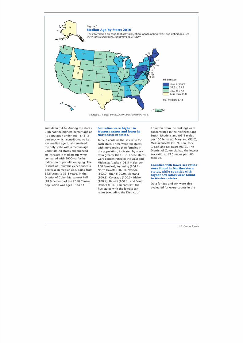
Maine and Vermont surpassedWest Virginia and Florida asthe states with the highestmedian age.

More variation in these distribu-

tions and measures can be seen

when looking at state-level com-

parisons. As expected rom theregional data, the states with the

highest median ages are located

largely in the Northeast, with the

exception o West Virginia and

Florida (Table 3 and Figure 5). In

both 1990 and 2000, West Virginia

and Florida had the highest median

age o all states. This trend shited

in 2010 due to increases in median

age between 2000 and 2010 or

the states o Maine, Vermont,

and New Hampshire. These threestates had the largest increases

in median age between 2000 and

2010, with an increase o 3.8

years in Vermont, 4.0 years in New

Hampshire, and 4.1 years in Maine.

Maine and Vermont surpassed West

Virginia and Florida as the states

with the highest median age.

There were seven states with amedian age over 40 years.

The ive states with the highest

median age in 2010 were Maine

(42.7), Vermont (41.5), West

Virginia (41.3), New Hampshire

(41.1), and Florida (40.7). In all,

there were seven states, the previ-

ous ive plus Connecticut and

Pennsylvania, with a median age

o 40 or higher. This was a shit

rom earlier decades, when all

states had a median age below 40.

Despite these shits in median age,

however, Florida and West Virginia

remained the states with the high-

est percentage o the population

age 65 and over, 17.3 percent and

16.0 percent, respectively.

Utah remained the state withthe lowest median age.

In contrast, the states with the

lowest median age (excluding the

District o Columbia) remained the

same as they were in 2000: Utah

(29.2), Texas (33.6), Alaska (33.8),

Figure 4.

Age Distribution and Median Age: 1960 to 2010

Sources: U.S. Census Bureau, 2010 Census Summary File 1, Census 2000 Summary File 1, 1990 Census Summary File 2C ,1980 Census Summary File 2C , 1970 Census of Population, Vol. 1, Characteristics of the Population, Chapter B, Table 50, and1960 Census of Population, Vol. 1, Characteristics of the Population, Chapter C, Table 156.

Under 18

37.2

35.3

32.9

30.0

28.1

29.5

18–44 45–64 65+Median age

1960

1970

1980

1990

2000

2010

(In percent. For information on confidentiality protection, nonsampling error, and definitions, see www.census.gov/prod/cen2010/doc/sf1.pdf)

24.0 36.5 26.4 13.0

25.7 39.9 22.0 12.4

25.6 43.2 18.6 12.6

28.1 40.9 19.6 11.3

34.3 35.3 20.6 9.8

35.9 34.8 20.3 9.0




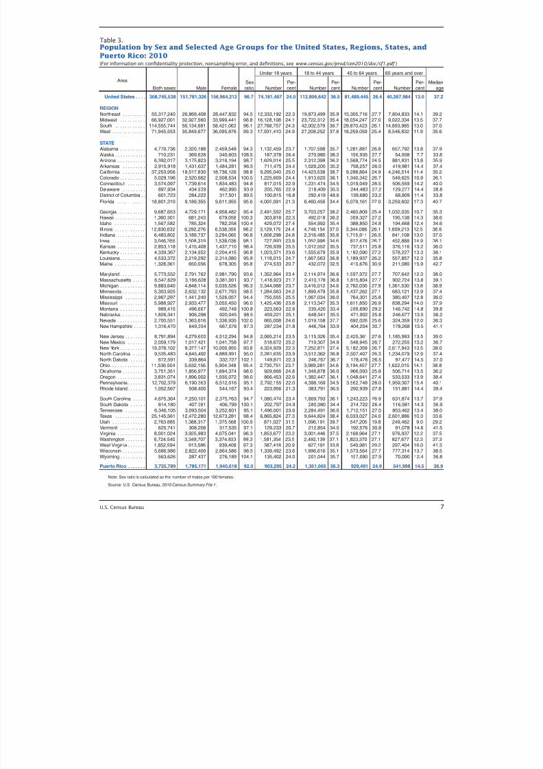
Table 3.Population by Sex and Selected Age Groups for the United States, Regions, States, and

Puerto Rico: 2010(For inormation on confdentiality protection, nonsampling error, and defnitions, see www.census.gov/prod/cen2010/doc/sf1.pdf )

Area

Both sexes Male FemaleSexratio

Under 18 years 18 to 44 years 45 to 64 years 65 years and over

MedianageNumber

Per-cent Number

Per-cent Number

Per-cent Number

Per-cent

United States 308,745,538 151,781,326 156,964,212 967 74,181,467 240 112,806,642 365 81,489,445 264 40,267,984 130 372

REGIONNortheast 55,317,240 26,869,408 28,447,832 945 12,333,192 223 19,873,499 359 15,305,716 277 7,804,833 141 392

Midwest 66,927,001 32,927,560 33,999,441 968 16,128,108 241 23,722,312 354 18,054,247 270 9,022,334 135 377South 114,555,744 56,134,681 58,421,063 961 27,788,757 243 42,002,579 367 29,870,423 261 14,893,985 130 370

West 71,945,553 35,849,677 36,095,876 993 17,931,410 249 27,208,252 378 18,259,059 254 8,546,832 119 356

STATEAlabama 4,779,736 2,320,188 2,459,548 943 1,132,459 237 1,707,598 357 1,281,887 268 657,792 138 379

Alaska 710,231 369,628 340,603 1085 187,378 264 270,980 382 196,935 277 54,938 77 338Arizona 6,392,017 3,175,823 3,216,194 987 1,629,014 255 2,312,398 362 1,568,774 245 881,831 138 359

Arkansas 2,915,918 1,431,637 1,484,281 965 711,475 244 1,026,205 352 758,257 260 419,981 144 374Caliornia 37,253,956 18,517,830 18,736,126 988 9,295,040 250 14,423,538 387 9,288,864 249 4,246,514 114 352

Colorado 5,029,196 2,520,662 2,508,534 1005 1,225,609 244 1,913,620 381 1,340,342 267 549,625 109 361

Connecticut 3,574,097 1,739,614 1,834,483 948 817,015 229 1,231,474 345 1,019,049 285 506,559 142 400Delaware 897,934 434,939 462,995 939 205,765 229 318,409 355 244,483 272 129,277 144 388

District o Columbia 601,723 284,222 317,501 895 100,815 168 292,419 486 139,680 232 68,809 114 338

Florida 18,801,310 9,189,355 9,611,955 956 4,002,091 213 6,460,456 344 5,079,161 270 3,259,602 173 407

Georgia 9,687,653 4,729,171 4,958,482 954 2,491,552 257 3,703,257 382 2,460,809 254 1,032,035 107 353Hawaii 1,360,301 681,243 679,058 1003 303,818 223 492,018 362 369,327 272 195,138 143 386

Idaho 1,567,582 785,324 782,258 1004 429,072 274 554,992 354 388,850 248 194,668 124 346

Illinois 12,830,632 6,292,276 6,538,356 962 3,129,179 244 4,748,154 370 3,344,086 261 1,609,213 125 366Indiana 6,483,802 3,189,737 3,294,065 968 1,608,298 248 2,318,485 358 1,715,911 265 841,108 130 370

Iowa 3,046,355 1,508,319 1,538,036 981 727,993 239 1,052,998 346 812,476 267 452,888 149 381Kansas 2,853,118 1,415,408 1,437,710 984 726,939 255 1,012,552 355 737,511 258 376,116 132 360

Kentucky 4,339,367 2,134,952 2,204,415 968 1,023,371 236 1,555,679 359 1,182,090 272 578,227 133 381

Louisiana 4,533,372 2,219,292 2,314,080 959 1,118,015 247 1,667,563 368 1,189,937 262 557,857 123 358Maine 1,328,361 650,056 678,305 958 274,533 207 432,072 325 410,676 309 211,080 159 427

Maryland 5,773,552 2,791,762 2,981,790 936 1,352,964 234 2,114,974 366 1,597,972 277 707,642 123 380

Massachusetts 6,547,629 3,166,628 3,381,001 937 1,418,923 217 2,410,178 368 1,815,804 277 902,724 138 391Michigan 9,883,640 4,848,114 5,035,526 963 2,344,068 237 3,416,012 346 2,762,030 279 1,361,530 138 389

Minnesota 5,303,925 2,632,132 2,671,793 985 1,284,063 242 1,899,479 358 1,437,262 271 683,121 129 374Mississippi 2,967,297 1,441,240 1,526,057 944 755,555 255 1,067,034 360 764,301 258 380,407 128 360

Missouri 5,988,927 2,933,477 3,055,450 960 1,425,436 238 2,113,347 353 1,611,850 269 838,294 140 379

Montana 989,415 496,667 492,748 1008 223,563 226 330,420 334 288,690 292 146,742 148 398Nebraska 1,826,341 906,296 920,045 985 459,221 251 648,541 355 471,902 258 246,677 135 362

Nevada 2,700,551 1,363,616 1,336,935 1020 665,008 246 1,019,158 377 692,026 256 324,359 120 363

New Hampshire 1,316,470 649,394 667,076 973 287,234 218 446,764 339 404,204 307 178,268 135 411

New Jersey 8,791,894 4,279,600 4,512,294 948 2,065,214 235 3,115,326 354 2,425,361 276 1,185,993 135 390

New Mexico 2,059,179 1,017,421 1,041,758 977 518,672 252 719,307 349 548,945 267 272,255 132 367New York 19,378,102 9,377,147 10,000,955 938 4,324,929 223 7,252,871 374 5,182,359 267 2,617,943 135 380

North Carolina 9,535,483 4,645,492 4,889,991 950 2,281,635 239 3,512,362 368 2,507,407 263 1,234,079 129 374

North Dakota 672,591 339,864 332,727 1021 149,871 223 246,767 367 178,476 265 97,477 145 370Ohio 11,536,504 5,632,156 5,904,348 954 2,730,751 237 3,989,281 346 3,194,457 277 1,622,015 141 388

Oklahoma 3,751,351 1,856,977 1,894,374 980 929,666 248 1,348,878 360 966,093 258 506,714 135 362

Oregon 3,831,074 1,896,002 1,935,072 980 866,453 226 1,382,447 361 1,048,641 274 533,533 139 384Pennsylvania 12,702,379 6,190,363 6,512,016 951 2,792,155 220 4,388,169 345 3,562,748 280 1,959,307 154 401

Rhode Island 1,052,567 508,400 544,167 934 223,956 213 383,791 365 292,939 278 151,881 144 394

South Carolina 4,625,364 2,250,101 2,375,263 947 1,080,474 234 1,669,793 361 1,243,223 269 631,874 137 379

South Dakota 814,180 407,381 406,799 1001 202,797 249 280,080 344 214,722 264 116,581 143 369

Tennessee 6,346,105 3,093,504 3,252,601 951 1,496,001 236 2,284,491 360 1,712,151 270 853,462 134 380

Texas 25,145,561 12,472,280 12,673,281 984 6,865,824 273 9,644,824 384 6,033,027 240 2,601,886 103 336Utah 2,763,885 1,388,317 1,375,568 1009 871,027 315 1,096,191 397 547,205 198 249,462 90 292

Vermont 625,741 308,206 317,535 971 129,233 207 212,854 340 192,576 308 91,078 146 415Virginia 8,001,024 3,925,983 4,075,041 963 1,853,677 232 3,001,446 375 2,168,964 271 976,937 122 375

Washington 6,724,540 3,349,707 3,374,833 993 1,581,354 235 2,492,139 371 1,823,370 271 827,677 123 373

West Virginia 1,852,994 913,586 939,408 973 387,418 209 627,191 338 540,981 292 297,404 160 413Wisconsin 5,686,986 2,822,400 2,864,586 985 1,339,492 236 1,996,616 351 1,573,564 277 777,314 137 385

Wyoming 563,626 287,437 276,189 1041 135,402 240 201,044 357 157,090 279 70,090 124 368

Puerto Rico 3,725,789 1,785,171 1,940,618 920 903,295 242 1,351,005 363 929,491 249 541,998 145 369

Note: Sex ratio is calculated as the number o males per 100 emales

Source: US Census Bureau, 2010 Census Summary File 1




and Idaho (34.6). Among the states,

Utah had the highest percentage o

its population under age 18 (31.5

percent), which contributed to itslow median age. Utah remained

the only state with a median age

under 30. All states experienced

an increase in median age when

compared with 2000—a urther

indication o population aging. The

District o Columbia experienced a

decrease in median age, going rom

34.6 years to 33.8 years. In the

District o Columbia, almost hal

(48.6 percent) o the 2010 Census

population was ages 18 to 44.

Sex ratios were higher inWestern states and lower inNortheastern states.

Table 3 contains the sex ratio or

each state. There were ten states

with more males than emales in

the population, indicated by a sex

ratio greater than 100. These states

were concentrated in the West and

Midwest: Alaska (108.5 males per

100 emales), Wyoming (104.1),

North Dakota (102.1), Nevada

(102.0), Utah (100.9), Montana

(100.8), Colorado (100.5), Idaho

(100.4), Hawaii (100.3), and South

Dakota (100.1). In contrast, theive states with the lowest sex

ratios (excluding the District o

Columbia rom the ranking) were

concentrated in the Northeast and

South: Rhode Island (93.4 males

per 100 emales), Maryland (93.6),Massachusetts (93.7), New York

(93.8), and Delaware (93.9). The

District o Columbia had the lowest

sex ratio, at 89.5 males per 100

emales.

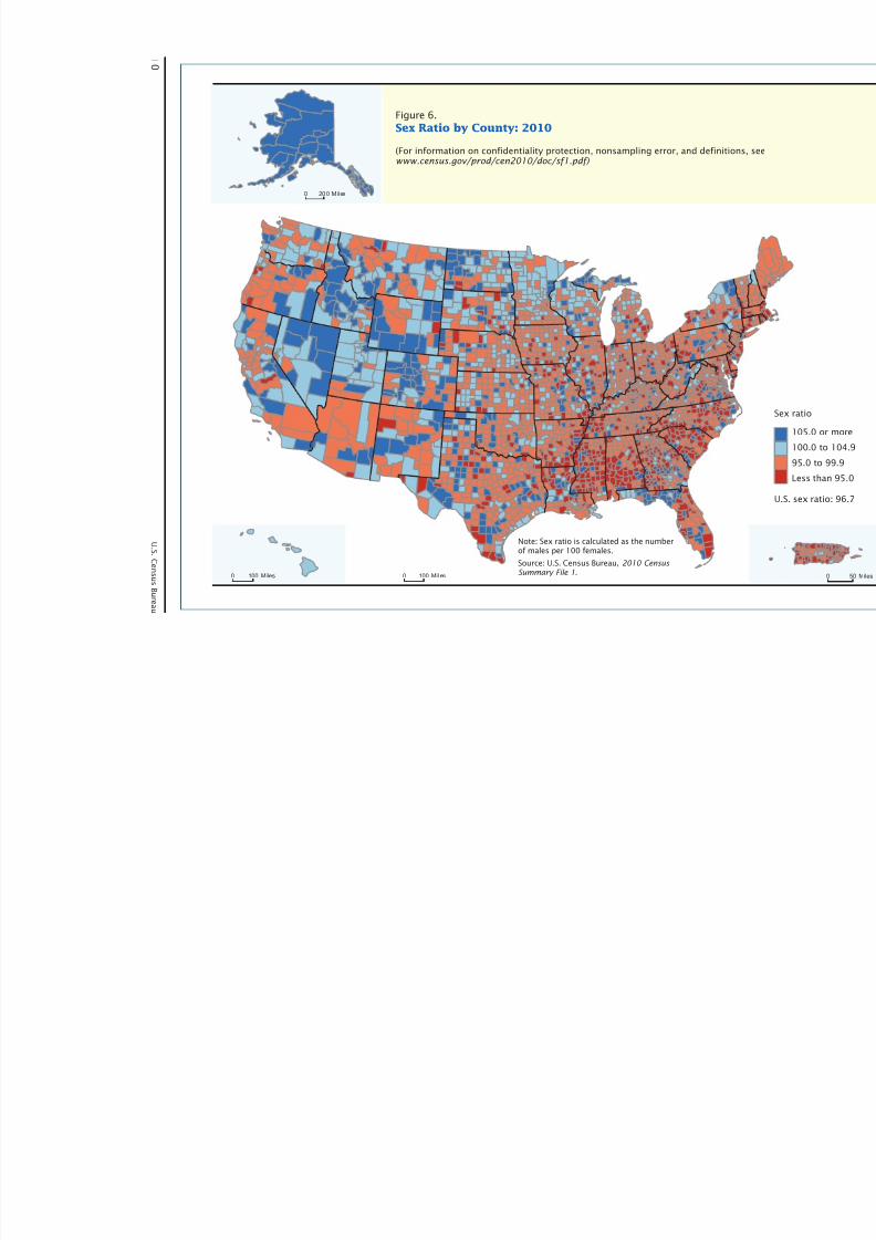
Counties with lower sex ratioswere found in Northeasternstates, while counties withhigher sex ratios were foundin Western states.

Data or age and sex were also

evaluated or every county in the

MT

AK

NM

OR MN

KS

SD

ND

MO

WA

FL

IL IN

WI NY

PA

MI

OH

IA

ME

MA

CT

AZ

HI

NV

TX

COCA

WY

UT

ID

NE

OK

GA

AR

AL

NC

MS

LA

TN

KYVA

SC

WV

RI

DEMDDC

NJ

Figure 5.

Median Age by State: 2010

VTNH

U.S. median: 37.2

Median age

40.0 or more

37.5 to 39.9

35.0 to 37.4

Less than 35.0

PR

(For information on confidentiality protection, nonsampling error, and definitions, see www.census.gov/prod/cen2010/doc/sf1.pdf)

Source: U.S. Census Bureau, 2010 Census Summary File 1.




United States. 5 These sex ratios

are illustrated in Figure 6, which

provides a map o sex ratios by

county. From this map, it is evi-

dent that counties in Northeastern

and Southern states tend to have

lower sex ratios, while counties

in Western and Midwestern states

tend to have higher sex ratios. In

2010, Alaska was the only state

where males outnumbered emales

in every county. In 2000, Alaska,

Hawaii, and Nevada had a greater

number o males than emales in

every county. In 2010, three states

had a sex ratio below 100 in every

county: Delaware, Maine, and

Rhode Island. Both Delaware and

Rhode Island had sex ratios that

were below the national level (96.7)

in every county.

Compared to 2000, therewere fewer counties in 2010where the female populationoutnumbered the malepopulation.

O the 3,143 total counties in the

United States, 1,096 o these (34.9

percent) had a sex ratio that was

less than the national sex ratio

o 96.7. In all, there were a total

o 2,089 counties (66.5 percent)with a sex ratio below 100, indi-

cating that the emale population

in the county outnumbered the

male population. This is a decrease

rom what was seen in 2000, when

5 The primary legal divisions o moststates are termed “counties.” In Louisiana,these divisions are known as parishes. InAlaska, which has no counties, the statisti-cally equivalent entities are census areas,city and boroughs (as in Juneau City andBorough), a municipality (Anchorage), andorganized boroughs. Census areas aredelineated cooperatively or data presenta-tion purposes by the state o Alaska and theU.S. Census Bureau. In our states (Maryland,Missouri, Nevada, and Virginia), there are oneor more incorporated places that are inde-pendent o any county organization and thusconstitute primary divisions o their states;these incorporated places are known as “inde-pendent cities” and are treated as equivalentto counties or data presentation purposes.The District o Columbia has no primarydivisions, and the entire area is consideredequivalent to a county and a state or datapresentation purposes.

73 percent o counties had a sex

ratio less than 100.

The county with the highest

sex ratio was Crowley County,

Colorado, with a sex ratio o 258.6,

indicating that there were more

than twice as many men as women

in the county. This high sex ratioresults rom the presence o a

state prison in Crowley County.

The lowest sex ratio was ound in

Pulaski County, Georgia, with a sex

ratio o 76.1. This low sex ratio

is partly due to the presence o a

state prison or women in Pulaski

County. The total population o

each o these counties, however,

was less than 12,500 people.

Among counties with at least

100,000 people, there were threecounties with a sex ratio greater

than 110: Kings County, Caliornia

(129.6), Onslow County, North

Carolina (115.7), and Pinal County,

Arizona (110.4). In both Kings

County and Pinal County, the high

sex ratios are due to the presence

o multiple correctional acilities

with majority male populations,

while Onslow County owes its high

sex ratio to the presence o a large

Marine Corps base that houses amostly male population. The lowest

sex ratios among counties with at

least 100,000 people were ound in

Hampshire County, Massachusetts

(88.0), Bronx County, New York

(88.3), and New York County, New

York (88.3). In Hampshire County,

the low sex ratio is inluenced by

the presence o several colleges,

two o which are women’s colleges.

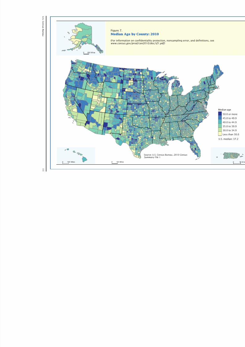
County-level median agesfollowed patterns seen at thestate level.

There was also variation at the

county level in the median age.

Figure 7 provides a map o median

age by county or all counties in

the United States. While median age

varied signiicantly among counties,

patterns emerge that are consis-

tent with indings reported earlier.

For example, counties in Florida,

New England, and the Appalachian

Mountain area tend to have higher

median ages, along with a band

o counties in the Great Plains

and Paciic Northwest. Counties

with lower median ages are ound

clustered along the United States–

Mexico border and within the states

o Utah and Alaska.

The number of counties witha median age over 40 grew,while those with a median ageless than 30 declined between2000 and 2010.

O the country’s 3,143 counties,

there were 1,683 counties with

a median age over 40. This is anincrease o more than double rom

Census 2000, where 734 counties

were ound to have a median age

over 40. In contrast, there were

only 93 counties with a median

age below 30, compared with 131

counties in 2000. The county with

the highest median age was Sumter

County, Florida (62.7), a county

with a population o just under

93,500, which is home to a large,

age-restricted retirement commu-nity. The lowest median age was

ound in the Wade Hampton Census

Area, Alaska (21.9), a county with a

population o less than 7,500.

Among counties with apopulation of at least 100,000,the counties with the highestmedian ages were found inFlorida.

Examining counties with a popula-

tion o at least 100,000 shows that

three counties, all in Florida, hada median age over 50: Charlotte

(55.9), Citrus (54.0), and Sarasota

(52.5). These were also the coun-

ties with the highest median

ages in 2000. Counties with a

low median age were consistent

between 2000 and 2010 as well.

The lowest median ages were



1 0

U . S . C en s u s

B ur e a u

0 100 Miles

0 20 0 M il es

0 100 Mil es

Figure 6.

Sex Ratio by County: 2010

(For information on confidentiality protection, nonsampling error, and definitiowww.census.gov/prod/cen2010/doc/sf1.pdf)

Note: Sex ratio is calculated as the numberof males per 100 females.




U . S . C en s u s

B ur e a u

1 1

0 100 Miles

0 200 Miles

0 100 Miles

Figure 7.

Median Age by County: 2010

(For information on confidentiality protection, nonsampling error, and definitiowww.census.gov/prod/cen2010/doc/sf1.pdf)





ound in Brazos County, Texas

(24.5), Utah County, Utah (24.6),

Cache County, Utah (25.5), Onslow

County, North Carolina (25.7), and

Clarke County, Georgia (25.9).

Three o these counties contain

large universities, which drive the

low median age in each county.

Brazos County, Texas, is home toTexas A&M University; Utah County,

Utah, contains Brigham Young

University; and the University o

Georgia is located in Clarke County,

Georgia. As mentioned previously,

Onslow County, North Carolina,

is home to a large Marine Corps

base with a primarily young, male

population. The presence o this

base contributes to the low median

age and high sex ratio in the

county. With the exception o CacheCounty, Utah, which was below

100,000 in population in 2000, all

o these counties were also in the

lowest ive or median age in 2000

as well.

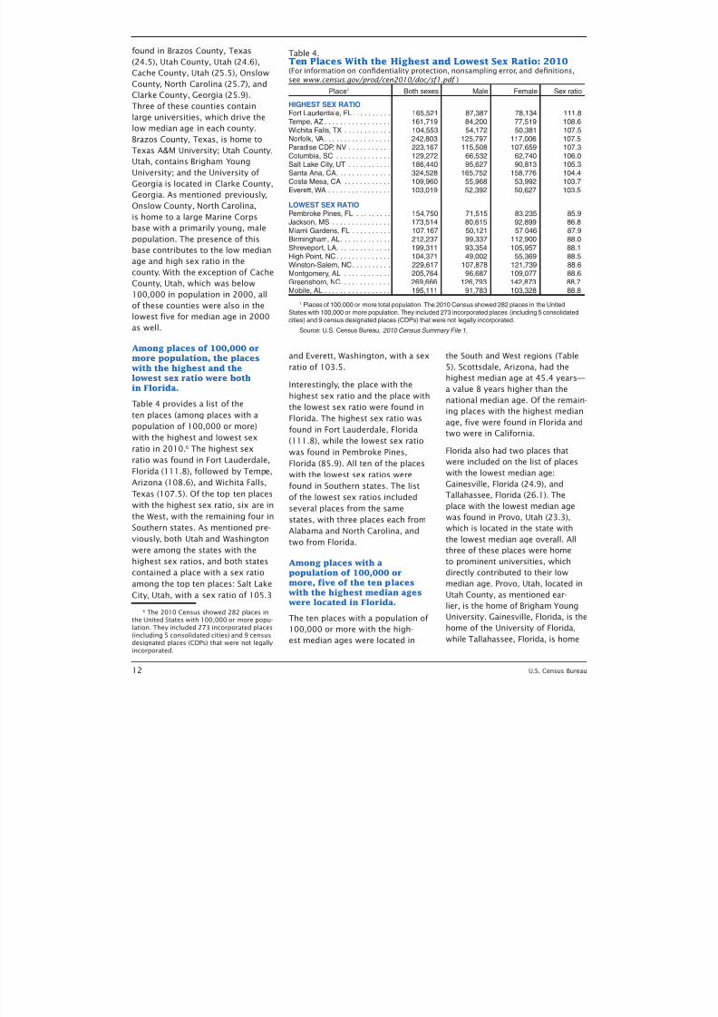
Among places of 100,000 ormore population, the placeswith the highest and thelowest sex ratio were bothin Florida.

Table 4 provides a list o the

ten places (among places with a

population o 100,000 or more)

with the highest and lowest sex

ratio in 2010.6 The highest sex

ratio was ound in Fort Lauderdale,

Florida (111.8), ollowed by Tempe,

Arizona (108.6), and Wichita Falls,

Texas (107.5). O the top ten places

with the highest sex ratio, six are in

the West, with the remaining our in

Southern states. As mentioned pre-

viously, both Utah and Washington

were among the states with thehighest sex ratios, and both states

contained a place with a sex ratio

among the top ten places: Salt Lake

City, Utah, with a sex ratio o 105.3

6 The 2010 Census showed 282 places inthe United States with 100,000 or more popu-lation. They included 273 incorporated places(including 5 consolidated cities) and 9 censusdesignated places (CDPs) that were not legallyincorporated.

and Everett, Washington, with a sex

ratio o 103.5.

Interestingly, the place with the

highest sex ratio and the place with

the lowest sex ratio were ound in

Florida. The highest sex ratio was

ound in Fort Lauderdale, Florida

(111.8), while the lowest sex ratio

was ound in Pembroke Pines,

Florida (85.9). All ten o the places

with the lowest sex ratios were

ound in Southern states. The list

o the lowest sex ratios included

several places rom the same

states, with three places each rom

Alabama and North Carolina, and

two rom Florida.

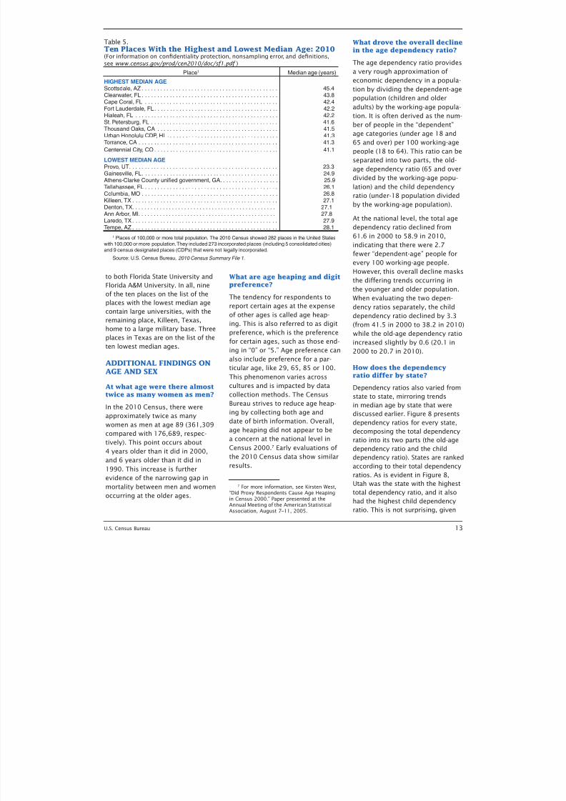
Among places with apopulation of 100,000 ormore, five of the ten placeswith the highest median ageswere located in Florida.

The ten places with a population o

100,000 or more with the high-

est median ages were located in

the South and West regions (Table

5). Scottsdale, Arizona, had the

highest median age at 45.4 years—

a value 8 years higher than the

national median age. O the remain-

ing places with the highest medianage, ive were ound in Florida and

two were in Caliornia.

Florida also had two places that

were included on the list o places

with the lowest median age:

Gainesville, Florida (24.9), and

Tallahassee, Florida (26.1). The

place with the lowest median age

was ound in Provo, Utah (23.3),

which is located in the state with

the lowest median age overall. All

three o these places were hometo prominent universities, which

directly contributed to their low

median age. Provo, Utah, located in

Utah County, as mentioned ear-

lier, is the home o Brigham Young

University. Gainesville, Florida, is the

home o the University o Florida,

while Tallahassee, Florida, is home

Table 4.Ten Places With the Highest and Lowest Sex Ratio: 2010(For inormation on confdentiality protection, nonsampling error, and defnitions,

see www.census.gov/prod/cen2010/doc/sf1.pdf )

Place1 Both sexes Male Female Sex ratio

HIGHEST SEX RATIOFort Lauderdale, FL 165,521 87,387 78,134 1118Tempe, AZ 161,719 84,200 77,519 1086Wichita Falls, TX 104,553 54,172 50,381 1075

Norolk, VA 242,803 125,797 117,006 1075Paradise CDP, NV 223,167 115,508 107,659 1073Columbia, SC 129,272 66,532 62,740 1060Salt Lake City, UT 186,440 95,627 90,813 1053Santa Ana, CA 324,528 165,752 158,776 1044Costa Mesa, CA 109,960 55,968 53,992 1037Everett, WA 103,019 52,392 50,627 1035

LOWEST SEX RATIOPembroke Pines, FL 154,750 71,515 83,235 859Jackson, MS 173,514 80,615 92,899 868Miami Gardens, FL 107,167 50,121 57,046 879Birmingham, AL 212,237 99,337 112,900 880Shreveport, LA 199,311 93,354 105,957 881High Point, NC 104,371 49,002 55,369 885Winston-Salem, NC 229,617 107,878 121,739 886

Montgomery, AL 205,764 96,687 109,077 886Greensboro, NC 269,666 126,793 142,873 887Mobile, AL 195,111 91,783 103,328 888

1 Places o 100,000 or more total population The 2010 Census showed 282 places in the United

States with 100,000 or more population They included 273 incorporated places (including 5 consolidated

cities) and 9 census designated places (CDPs) that were not legally incorporated

Source: US Census Bureau, 2010 Census Summary File 1.




to both Florida State University and

Florida A&M University. In all, nine

o the ten places on the list o the

places with the lowest median age

contain large universities, with the

remaining place, Killeen, Texas,

home to a large military base. Three

places in Texas are on the list o the

ten lowest median ages.

ADDITIONAL FINDINGS ONAGE AND SEX

At what age were there almosttwice as many women as men?

In the 2010 Census, there were

approximately twice as many

women as men at age 89 (361,309

compared with 176,689, respec-tively). This point occurs about

4 years older than it did in 2000,

and 6 years older than it did in

1990. This increase is urther

evidence o the narrowing gap in

mortality between men and women

occurring at the older ages.

What are age heaping and digitpreference?

The tendency or respondents to

report certain ages at the expense

o other ages is called age heap-

ing. This is also reerred to as digitpreerence, which is the preerence

or certain ages, such as those end-

ing in “0” or “5.” Age preerence can

also include preerence or a par-

ticular age, like 29, 65, 85 or 100.

This phenomenon varies across

cultures and is impacted by data

collection methods. The Census

Bureau strives to reduce age heap-

ing by collecting both age and

date o birth inormation. Overall,

age heaping did not appear to bea concern at the national level in

Census 2000.7 Early evaluations o

the 2010 Census data show similar

results.

7 For more inormation, see Kirsten West,“Did Proxy Respondents Cause Age Heapingin Census 2000.” Paper presented at theAnnual Meeting o the American StatisticalAssociation, August 7–11, 2005.

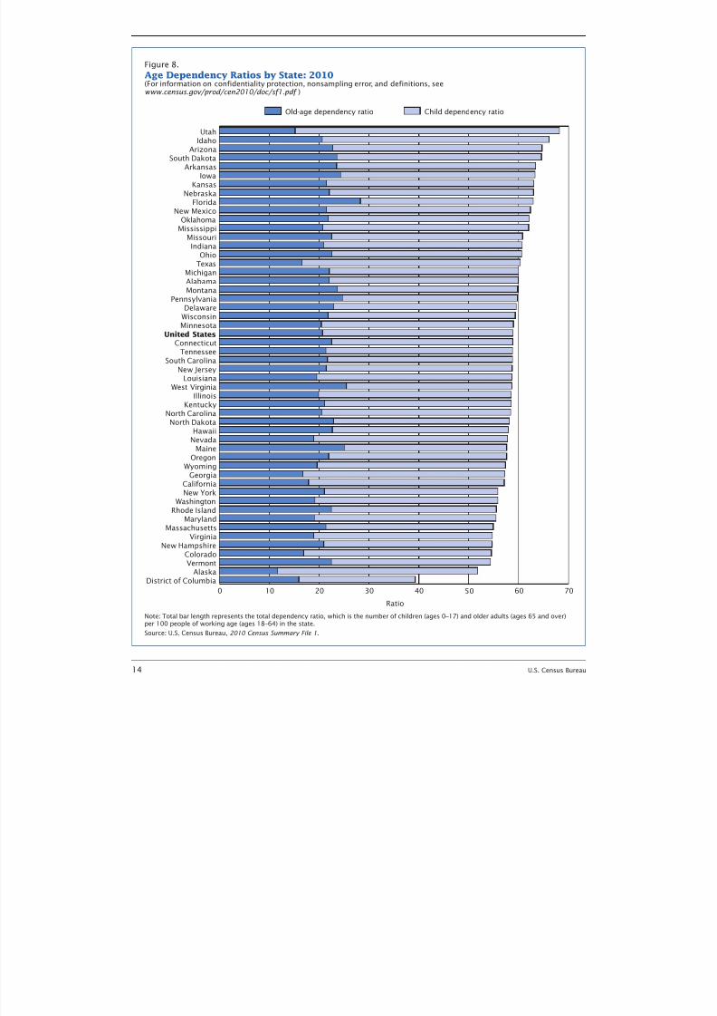
What drove the overall declinein the age dependency ratio?

The age dependency ratio provides

a very rough approximation o

economic dependency in a popula-

tion by dividing the dependent-age

population (children and older

adults) by the working-age popula-tion. It is oten derived as the num-

ber o people in the “dependent”

age categories (under age 18 and

65 and over) per 100 working-age

people (18 to 64). This ratio can be

separated into two parts, the old-

age dependency ratio (65 and over

divided by the working-age popu-

lation) and the child dependency

ratio (under-18 population divided

by the working-age population).

At the national level, the total agedependency ratio declined rom

61.6 in 2000 to 58.9 in 2010,

indicating that there were 2.7

ewer “dependent-age” people or

every 100 working-age people.

However, this overall decline masks

the diering trends occurring in

the younger and older population.

When evaluating the two depen-

dency ratios separately, the child

dependency ratio declined by 3.3

(rom 41.5 in 2000 to 38.2 in 2010)while the old-age dependency ratio

increased slightly by 0.6 (20.1 in

2000 to 20.7 in 2010).

How does the dependencyratio differ by state?

Dependency ratios also varied rom

state to state, mirroring trends

in median age by state that were

discussed earlier. Figure 8 presents

dependency ratios or every state,

decomposing the total dependencyratio into its two parts (the old-age

dependency ratio and the child

dependency ratio). States are ranked

according to their total dependency

ratios. As is evident in Figure 8,

Utah was the state with the highest

total dependency ratio, and it also

had the highest child dependency

ratio. This is not surprising, given

Table 5.Ten Places With the Highest and Lowest Median Age: 2010(For inormation on confdentiality protection, nonsampling error, and defnitions,

see www.census.gov/prod/cen2010/doc/sf1.pdf )

Place1 Median age (years)

HIGHEST MEDIAN AGEScottsdale, AZ 454Clearwater, FL 438Cape Coral, FL 424

Fort Lauderdale, FL 422Hialeah, FL 422St Petersburg, FL 416Thousand Oaks, CA 415Urban Honolulu CDP, HI 413Torrance, CA 413

Centennial City, CO 411

LOWEST MEDIAN AGEProvo, UT 233Gainesville, FL 249Athens-Clarke County unifed government, GA 259Tallahassee, FL 261Columbia, MO 268Killeen, TX 271Denton, TX 271

Ann Arbor, MI 278Laredo, TX 279Tempe, AZ 281

1 Places o 100,000 or more total population The 2010 Census showed 282 places in the United States

with 100,000 or more population They included 273 incorporated places (including 5 consolidated cities)

and 9 census designated places (CDPs) that were not legally incorporated

Source: US Census Bureau, 2010 Census Summary File 1




Figure 8.

Age Dependency Ratios by State: 2010(For information on confidentiality protection, nonsampling error, and definitions, seewww.census.gov/prod/cen2010/doc/sf1.pdf )

Note: Total bar length represents the total dependency ratio, which is the number of children (ages 0–17) and older adults (ages 65 and over)per 100 people of working age (ages 18–64) in the state.


Old-age dependency ratio Child dependency ratio

0 10 20 30 40 50 60 70

District of ColumbiaAlaska

VermontColorado

New HampshireVirginia

MassachusettsMaryland

Rhode IslandWashington

New YorkCalifornia

GeorgiaWyoming

OregonMaine

NevadaHawaii

North DakotaNorth Carolina

KentuckyIllinois

West VirginiaLouisiana

New JerseySouth Carolina

TennesseeConnecticut

United States

MinnesotaWisconsinDelaware

PennsylvaniaMontanaAlabamaMichigan

TexasOhio

IndianaMissouri

MississippiOklahoma

New MexicoFlorida

NebraskaKansas

IowaArkansas

South DakotaArizona

IdahoUtah

Ratio




that Utah was the state with the

lowest median age, as mentioned

previously. The lowest child depen-

dency ratio was ound in Vermont,

a state that also had a high median

age. Excluding the District o

Columbia, the state with the lowest

total dependency ratio was Alaska.

Alaska was also the state with thelowest old-age dependency ratio,

while the state with the highest old-

age dependency ratio was Florida,

again matching trends in median

age mentioned previously or these

states. The District o Columbia had

the lowest dependency ratio overall.

ABOUT THE 2010 CENSUS

Why was the 2010 Censusconducted?

The U.S. Constitution mandates

that a census be taken in the

United States every 10 years. This

is required in order to determine

the number o seats each state

is to receive in the U.S. House o

Representatives. Age data are used

to determine the voting age popu-

lation (age 18 and older) or use in

the legislative redistricting process.

Why did the 2010 Census ask

the questions on age and sex?

The Census Bureau collects data on

age and sex to support a variety

o legislative and program require-

ments. These data are also used to

aid in allocating unds rom ederal

programs, in particular to programs

targeting speciic age groups. For

example, age data are used to

calculate the proportion o school-

aged children in each district in

order to properly allocate unds or

education.

How are age and sex databeneficial?

All levels o government need

inormation on age and sex to

implement and evaluate programs,

such as the Equal Employment

Opportunity Act, the Civil Rights

Act, the Women’s Educational EquityAct, the Older Americans Act, the

Juvenile Justice and Delinquency

Prevention Act, and the Job Training

Partnership Act. Age and sex data

are used by the Department o

Veterans Aairs, the Department

o Education, the Department o

Health and Human Services, and

the Equal Employment Opportunity

Commission, among others, to aid

in planning and development o

services.

Other equally important uses or

census age and sex data are in

planning adequate schools or

the school age population and to

determine unding distributions or

schools and planning or numerous

social services such as highways,

hospitals, health services, and

services or the older population.

Census age data are also an impor-

tant source o inormation on popu-

lation aging, such as measuremento people eligible or Social Security

and Medicare beneits. In addition

to these public uses o census data,

census data can also be used by

private organizations. For example,

census data can help researchers

studying trends related to mortality

and population aging or help small

business owners in planning where

to best locate their businesses to it

the needs o the community.

FOR MORE INFORMATION

For more inormation on age and

sex in the United States, visit the

U.S. Census Bureau’s Internet sites

at <www.census.gov/population

/www/socdemo/age/> and

<www.census.gov/population

/www/socdemo/women.html>.

Data on age and sex rom the

2010 Census Summary File 1 pro-

vide inormation at the state level

and below and are available on

the Internet at <actinder2

.census.gov/main.html> and on

DVD. Inormation on conidential-

ity protection, nonsampling error,

and deinitions is available on the

Census Bureau’s Internet site at

<www.census.gov/prod/cen2010

/doc/s1.pd >.

Inormation on other population

and housing topics is presented

in the 2010 Census Bries series,

located on the U.S. Census Bureau’s

Web site at <www.census.gov

/prod/cen2010/>. This series

presents inormation about race,

Hispanic origin, age, sex, house-

hold type, housing tenure, and peo-

ple who reside in group quarters.

For more inormation about the2010 Census, including data prod-

ucts, call the Customer Services

Center at 1-800-923-8282. You

can also visit the Census Bureau’s

Question and Answer Center at

<ask.census.gov> to submit your

questions online.

http://www.census.gov/population/www/socdemo/age/


http://www.census.gov/population/www/socdemo/women.html


http://factfinder2.census.gov/main.html


http://www.census.gov/prod/cen2010/doc/sf1.pdf


http://www.census.gov/prod/cen2010/


http://ask.census.gov/

http://ask.census.gov/













U.S. Department of Commerce

Economics and Statistics Administration

U.S. CENSUS BUREAU

Washington, DC 20233

OFFICIAL BUSINESS

Penalty f or Private Use $300

FIRST-CLASS MAILPOSTAGE & FEES PAIDU.S. Census Bureau

Permit No. G-58

Documents

US Age and Sex Composition