Embed Size (px)
Citation preview

Policy Research Working Paper 8530
Urbanization in Kazakhstan
Desirable Cities, Unaffordable Housing, and the Missing Rental Market
William Seitz
Poverty and Equity Global Practice July 2018
WPS8530P
ublic
Dis
clos
ure
Aut
horiz
edP
ublic
Dis
clos
ure
Aut
horiz
edP
ublic
Dis
clos
ure
Aut
horiz
edP
ublic
Dis
clos
ure
Aut
horiz
ed

Produced by the Research Support Team
Abstract
The Policy Research Working Paper Series disseminates the findings of work in progress to encourage the exchange of ideas about development issues. An objective of the series is to get the findings out quickly, even if the presentations are less than fully polished. The papers carry the names of the authors and should be cited accordingly. The findings, interpretations, and conclusions expressed in this paper are entirely those of the authors. They do not necessarily represent the views of the International Bank for Reconstruction and Development/World Bank and its affiliated organizations, or those of the Executive Directors of the World Bank or the governments they represent.
Policy Research Working Paper 8530
Kazakhstan’s cities are hubs of economic opportunity and prosperity. But despite the government’s ambitious targets, the pace of urbanization remains slow. This study focuses on two key constraints: (i) the very high cost of living in Kazakhstan’s cities, and (ii) the near absence of a rental housing market outside the capital, Astana. The findings show that the two urban centers of Almaty and Astana are 190 and 240 percent more expensive to live in than the national average. Housing is the primary driver of the dis-parity: after adjusting for inflation, housing costs tripled in Astana and quadrupled in Almaty between 2001 and 2015. As a result, housing costs for the local population in these
areas are more unaffordable than famously exclusive cities such as San Francisco and Vancouver. Demand elasticities from 2015 imply that in the current environment, rural and low-income households are especially unlikely to relocate to high-priced areas where employment prospects are better and average incomes are higher. Regional convergence in wage rates remains slow, but appears to be proceeding most quickly in Astana, where rental housing is most prevalent. The findings suggest that high rates of home ownership and the high cost of living in cities lead to exclusion of lower-income households and restrain economic growth.
This paper is a product of the Poverty and Equity Global Practice. It is part of a larger effort by the World Bank to provide open access to its research and make a contribution to development policy discussions around the world. Policy Research Working Papers are also posted on the Web at http://www.worldbank.org/research. The author may be contacted at [email protected].
Urbanization in Kazakhstan Desirable Cities, Unaffordable Housing, and the
Missing Rental Market
William Seitz
Economist Poverty and Equity The World Bank
2
Tables Table 1: 2015 HBS Sample Description by Quarter and Region ................................................................................ 8 Table 2: Sample Size by Location ..................................................................................................................................... 9 Table 3: Median Reported Rental and Purchase Values for Housing in 1000s of Tenge, HBS 2015 ................. 10 Table 4: OLS Regression detailing association between rent estimate and housing quality indicators ............... 12 Table 5: Estimated Food-based, Food + Rent-based, and Food + Standard Rent-based Indexes by Region and by Rural and Urban areas (National Average = 100%) ...................................................................................... 19 Table 6: Kazakhstan Cities Median Multiple Affordability Measures vs. International Cities ............................. 23 Table 7: Log-Log OLS Regressions (Dependent Variable = ln(imputed rent)) ..................................................... 27 Table 8: Comparison of the Observed Share of Imputed Rent in Total Consumption (left) vs. Simulated Rent using average Urban Imputed Rent (Right) .................................................................................................................. 35 Table 9: Comparison of Index of Imputed Rent (left) to Index of Dwelling Value (right) .................................. 35 Table 10: Average Imputed Rent Paid vs. Average Imputed "Standard" rent in 1000s of Tenge, HBS 2015 .. 37 Table 11: Rent Estimates in Almaty and Astana as a Share of Average/25th Percentile Household Income (2006-2015) ........................................................................................................................................................................ 38
Figures Figure 1: Share of Population living in Households with a Connection to Central Piped Water in Urban (Left) and Rural Areas (Right) by Consumption Quintile ....................................................................................................... 4 Figure 2: Real Existing Housing Sales Prices (right, 2001=100) ................................................................................. 5 Figure 3: Sales vs. Rental Value in 1000s of Tenge for 2015 ..................................................................................... 11 Figure 4: Rural vs. Urban Food-based Spatial Deflation Index................................................................................. 15 Figure 5: Food Index Value by District (left), Food Index Hot-Cold Spots (right) ............................................... 16 Figure 6: Poverty Rates at $5-a-day 2005 PPP with and without Spatial Food Price Deflation (left) ................. 17 Figure 7: Index of Imputed Rent (left), Hot-Cold Spot Map of Imputed Rent (right) ......................................... 20 Figure 8: Imputed Rent Share of Total Consumption, 2015 ..................................................................................... 22 Figure 9: Budget Share Allocated to Rent vs. Simulated Share using Average Urban Rent (left), Mapping of Simulated Rent Share using Average Urban Rent (right) ........................................................................................... 24 Figure 10: Growth Incidence Curve for 2006-2015 (Left), Approximation of Engel Curve for Imputed Rent and Total Consumption (Right) ..................................................................................................................................... 28 Figure 11: Home Ownership Rate by Country, 2015 .................................................................................................. 29 Figure 12: The Share of Owner-Occupied Out of Total Occupied Housing by Region in 2015 ........................ 31 Figure 13: Location-Specific Wage Residual (National Average=0%) ..................................................................... 32 Figure 14: Gini Coefficient by Year ............................................................................................................................... 39

3
1. Introduction
Urbanization is one of the pillars of Kazakhstan’s national “2050” development strategy (www.strategy2050.kz).
This focus is well aligned with decades of experience from around the world. Economic growth and
employment opportunities in cities have powered massive rural-to-urban migration and an historic reduction
in global poverty over the past century. Urbanization is strongly associated with poverty reduction and higher
living standards (Ravallion et. al., 2007), and there are compelling theoretical reasons to expect rural-to-urban
migration will be pro-poor (Ravaillion, 2002). While supporting the welfare of the rural population is also a
crucial component to Kazakhstan’s national development strategy, enabling cities to grow and thrive will play
a key role in achieving the government’s long-term development objectives for rural and urban areas alike.
Globally, cities and towns are hubs of prosperity—more than 80 percent of economic activity is produced in
cities by just over half of the world’s population (World Bank, 2013). Urban areas feature higher-paying jobs,
greater diversity of economic activities, and substantially higher average productivity. These effects are driven
not only by the benefits of agglomeration for firms and workplaces, but also by workers taking part in the
deeper and more specialized labor markets common in urban areas.
The cost of providing basic services in cities is also much lower. In 2013, the global average cost of providing
piped water was only $0.70–$0.80 per cubic meter in urban areas, compared to about $2 in sparsely populated
areas. In Kazakhstan, as in most middle-income countries, the high cost of providing services in rural areas
leads to significant discrepancies in service quality when compared to urban areas (Figure 1). But the high cost
of providing services to sparsely populated locations is particularly relevant in Kazakhstan, the world’s 9th largest
country, covering an area roughly the size of Western Europe. With only 6.5 people per kilometer on average
– ranging to as few as 2.7 people per kilometer in Aktobe region – Kazakhstan is the 10th least densely populated
country.
4
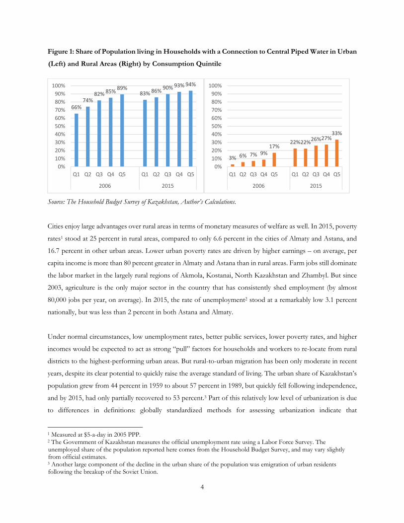
Figure 1: Share of Population living in Households with a Connection to Central Piped Water in Urban
(Left) and Rural Areas (Right) by Consumption Quintile
Source: The Household Budget Survey of Kazakhstan, Author’s Calculations.
Cities enjoy large advantages over rural areas in terms of monetary measures of welfare as well. In 2015, poverty
rates1 stood at 25 percent in rural areas, compared to only 6.6 percent in the cities of Almaty and Astana, and
16.7 percent in other urban areas. Lower urban poverty rates are driven by higher earnings – on average, per
capita income is more than 80 percent greater in Almaty and Astana than in rural areas. Farm jobs still dominate
the labor market in the largely rural regions of Akmola, Kostanai, North Kazakhstan and Zhambyl. But since
2003, agriculture is the only major sector in the country that has consistently shed employment (by almost
80,000 jobs per year, on average). In 2015, the rate of unemployment2 stood at a remarkably low 3.1 percent
nationally, but was less than 2 percent in both Astana and Almaty.
Under normal circumstances, low unemployment rates, better public services, lower poverty rates, and higher
incomes would be expected to act as strong “pull” factors for households and workers to re-locate from rural
districts to the highest-performing urban areas. But rural-to-urban migration has been only moderate in recent
years, despite its clear potential to quickly raise the average standard of living. The urban share of Kazakhstan’s
population grew from 44 percent in 1959 to about 57 percent in 1989, but quickly fell following independence,
and by 2015, had only partially recovered to 53 percent.3 Part of this relatively low level of urbanization is due
to differences in definitions: globally standardized methods for assessing urbanization indicate that
1 Measured at $5-a-day in 2005 PPP. 2 The Government of Kazakhstan measures the official unemployment rate using a Labor Force Survey. The unemployed share of the population reported here comes from the Household Budget Survey, and may vary slightly from official estimates. 3 Another large component of the decline in the urban share of the population was emigration of urban residents following the breakup of the Soviet Union.
66%74%
82% 85%89%
83% 86%90% 93% 94%
0%
10%
20%
30%
40%
50%
60%
70%
80%
90%
100%
Q1 Q2 Q3 Q4 Q5 Q1 Q2 Q3 Q4 Q5
2006 2015
3% 6% 7% 9%17%
22%22%26%27%
33%
0%
10%
20%
30%
40%
50%
60%
70%
80%
90%
100%
Q1 Q2 Q3 Q4 Q5 Q1 Q2 Q3 Q4 Q5
2006 2015

5
Kazakhstan’s urban population share may be somewhat higher than official estimates suggest, as are those of
the other central Asian countries.
However, a larger determinant of slow urbanization is remarkably low rates of internal migration. Rural-to-
urban migration accounted for only one-fifth of urban population growth between 2010 and 2015 (OECD,
2017).4 Only about 1.7 to 2.3 percent of the population move between regions within the country in a given
year.5 This is a much lower share than in many developed economies. For the US, the comparable figure is 11
percent, in Canada it is 14 percent.6 Growth projections from the UN predict that the urban share of
Kazakhstan’s total population is expected to be about 65 percent by 2050, well short of the government’s
official target of 70 percent.
Why is urbanization proceeding so slowly? In Kazakhstan, as in many countries, one explanation is that is it
very expensive to live in cities. In 2006, a single year’s growth in housing prices in Astana and Almaty outpaced
income growth over the entire period from 2006 to 2015 (Figure 2).
Figure 2: Real Existing Housing Sales Prices (right, 2001=100)
Source: Existing housing sales prices from KazStat, adjusted by the Author using the national CPI.
4 The large majority was due to natural population growth within cities. 5 About 300,000 to 400,000 people. 6 The Russian Federation, which shares many structural characteristics with Kazakhstan and has famously high costs of living in the capital city, has a similarly low rate of internal migration of about 2.6 percent.
100
200
300
400
500
600
700
800
900
1000
1100
Almaty Astana National

6
The gap in prices between cities and outlying regions in Kazakhstan is one of the largest in the region of Europe
and Central Asia. For food, the premium in Almaty was 15 percent above the national average in 2015 – off a
peak of as high as 20 percent in 2008. But the divergence in the cost of housing between rural and urban areas
is even more stark. On average, the cost of housing consumed (as measured by imputed rents) is 310 percent
higher than the national average in the city of Almaty, and about 460 percent higher in Astana.
The large differences in housing costs are due in part to the rapid and volatile appreciation of home values seen
in recent years. Official statistics show that real housing prices (measured mostly in urban areas) rose six-fold
between 2001 and 2016. In 2016, real housing prices in the city of Astana were three-times higher than in 2001,
and prices more than quadrupled in Almaty over the same period.7 Although slower than the national average,
rising housing prices in Almaty and Astana have been particularly remarkable given that these areas were already
much more expensive than other parts of the country. Urban housing price growth has also been extraordinarily
unstable: in real terms, prices rose by an average of more than 50 percent per year between 2001 and 2007, only
to fall by more than 60 percent in real terms over the following five years.
The sensitivity of people to these changes in prices and incomes will play a decisive role determining the
urbanization trajectory of the country. This paper investigates both using official microdata from the household
budget survey of Kazakhstan. The results show that the responsiveness of housing demand to changes in
income is slightly higher than other countries on average – with an elasticity to income of about .66. This means
that if incomes in the country grow, on average, housing demand would be expected to rise by 34 percent less
than the increase in income, on average. However, as housing prices rise, theory dictates that housing demand
will fall.8 The findings suggest that housing demand is quite responsive to price in Kazakhstan, with an elasticity
of about -.85 at the national level. Thus, taken together, the results indicate that the price elasticity dominates
the income elasticity in absolute terms. In other words, if over the coming years both incomes and prices were
to rise by 10 percent, the price effect would overwhelm the income effect, and on net, demand for housing
would fall.
This greater sensitivity to housing prices would be expected to be strongest among low-income households
that are budget constrained. For them, theory would predict that rising urban housing costs in cities such as
Astana and Almaty would provide a strong incentive to leave. This lines up well with recent demographic
statistics: increasingly, the people who can afford to live in sought after urban areas are well-educated high
earners. In Astana, the share of the workforce who completed a tertiary degree increased from 43 percent in
7 In nominal terms prices increased by factors of about 12 and 15, respectively. 8 Except in rare and extreme cases for specific housing markets.

7
2006 to 51 percent in 2015. In the city of Almaty, the share grew from 45 percent to 61 percent over the same
period.
But perhaps the most remarkable feature of the housing market in Kazakhstan is that, per official statistics,
rental housing is nearly non-existent outside of Astana. At around 95 percent, Kazakhstan has one of the
highest home-ownership rates in the world. A high ownership rate is one of the primary drivers of low mobility
identified in the literature. Thus, despite potential advantages in terms of income and amenities, many potential
migrants in Kazakhstan would not be able to sequence the steps of moving to a city in the absence of affordable
rental housing options.
These trends have large social implications for Kazakhstan’s future economic growth. Ganong and Shoag
(2017) show that disproportionate increases in housing prices in high-income places can lead to a dramatic
decline in the rate of income convergence across states and in population flows to high-income places. The
growing inaccessibility of Astana and Almaty also echoes the literature on affordability and the dangers of what
Gyourko, et al. (2006) refer to as the “superstar city” phenomenon. Their conclusion that “living in a superstar
city is like owning a scarce luxury good” aptly describes the state of the housing market in urban Kazakhstan.
Albouy et al. (2016) find that for many countries, such exclusive cities are much more expensive for the poor,
and that the current trend of rising rents over time, such as in Kazakhstan, has been one of the primary drivers
of increased real-income inequality in the United States.9
The remainder of the paper is organized as follows: section 2 describes the data and section 3 describes the
creation of spatial price indexes and for food and housing. Section 4 provides estimates of the affordability of
housing. The results presented in this section suggest that housing in key urban centers in Kazakhstan is highly
unaffordable using several standard measures of affordability, and that this likely impedes internal migration.
Estimates and correlates of housing demand are derived in section 5 using survey micro-data. These estimates
show that housing consumers are currently quite price sensitive (an increase in the price equates to a nearly
equal reduction in consumption). However, consumers are also responsive to income: a 10 percent increase in
income is associated with a 6.6 percent increase in housing consumption. These results in combination suggest
that rural/poor incomes would need to rise by a much larger amount than the cost of housing to induce a faster
pace of internal mobility and urbanization. Regional convergence, and the relationship between home
ownership, housing costs, and the labor market is discussed in section 6. The discussion focuses on how the
9 Appendix E reports the effect of housing costs on inequality for Kazakhstan, which similarly highlights this effect.

8
high cost of housing can impede regional “catch up” growth in rural areas, and reduce potential economic
growth in rural and urban areas alike. Section 7 concludes.
2. Data
This study draws mainly from the 2014/2015 rounds of the Kazakhstan Household Budget Survey (HBS),
conducted by the Statistics Agency of the Republic of Kazakhstan. For household consumption, the survey is
nationally representative, representative at the oblast (region) level, and separately representative for rural and
urban areas. The survey uses a stratified sample design with strata corresponding to 16 regions crossed by their
urban and rural areas (except for Almaty and Astana cities, which are entirely urban). A complete consumption
module (using a diary approach) is gathered in the HBS, covering both food and non-food items. Information
on household composition, income, employment, and related topics is also collected. In 2015, the data covered
all four quarters of the year, including 47,329 household-observations (about 12,000 unique households in a
panel design) and 169,091 individual-observations (about 42,000 individuals, also interviewed in a panel).
Results can be matched to the district and PSU level, but official statistics are usually reported for the regional
level only. Table 1 provides a description of the HBS sample composition.
Table 1: 2015 HBS Sample Description by Quarter and Region
Quarter Households Individuals Urban Households
Rural Households
Urban Individuals
Rural Individuals
Q1 11985 42706 6195 5790 20132 22574
Q2 11862 42376 6098 5764 19869 22507
Q3 11769 42095 6033 5736 19684 22411
Q4 11713 41914 6000 5713 19578 22336 Total 47329 169091 24326 23003 79263 89828
Source: The Household Budget Survey of Kazakhstan, Author’s Calculations.

9
Table 2: Sample Size by Location
Region Households Individuals Urban Households
Rural Households
Urban Individuals
Rural Individuals
Akmola 3318 10911 1405 1913 4260 6651
Aktobe 3356 13324 1436 1920 5328 7996
Almaty 2835 10179 935 1900 2949 7230
Atyrau 2158 9608 1198 960 5064 4544
West_Kaz 2590 9487 931 1659 3119 6368
Jambyl 2738 10572 1071 1667 3664 6908
Karaganda 3814 12456 2390 1424 7030 5426
Kostanay 3151 9099 1399 1752 3731 5368
Kyzylorda 2394 12310 956 1438 5032 7278
Mangystau 2397 10361 1320 1077 4956 5405
South_Kaz 3120 14128 1200 1920 4544 9584
Pavlodar 3360 10672 1440 1920 4312 6360
North_Kaz 2621 7710 1068 1553 2877 4833
East_Kaz 3539 10068 1639 1900 4191 5877
Astana_city 2588 8932 2588 0 8932 0 Almaty_city 3350 9274 3350 0 9274 0
Source: The Household Budget Survey of Kazakhstan, Author’s Calculations.
The analyses discussed in this paper primarily use the data from two modules of the survey; (i) the diary of food
consumed, and (ii) the dwelling characteristics and imputed rents of households. The food diary is collected
over two-week periods each quarter for each participating household. The main respondent is the household
member most knowledgeable regarding household expenditure. The statistical agency aggregates responses to
the quarterly level in a public-use data file.
The HBS module on living conditions and the cost of housing was collected in January 2015. Two separate
measures of the cost of housing were reported.10 The first was a measure of monthly rent defined as either: i)
rent paid, or the response provided by the respondent to the following question: “Could you please assess how
much would you pay per month, if you rented your principal accommodation”. In Kazakhstan, about 95
percent of households own their dwelling, and in only about 3 percent of cases were actual rental payments
observed. However, robustness analyses conducted by comparing the average of imputed vs. actual rent
payments by dwelling types indicates a reasonably strong relationship between the two measures, albeit they
are based a small number of observations. The second measure reported in the dwelling module is an estimate
the cost of purchasing a house using the question “Could you please assess for how much you could sell your
10 One additional measure of rent is described in a procedure described in greater detail below.

10
principal accommodation”. Comparing across these two indicators is on average consistent across regions and
rural/urban areas (Table 3).
Table 3: Median Reported Rental and Purchase Values for Housing in 1000s of Tenge, HBS 2015
All Urban Rural
Median Imputed Rent
Median Home Purchase
Median Imputed Rent
Median Home Purchase
Median Imputed Rent
Median Home Purchase
Akmola 240 2700 360 4400 120 900 Aktobe 300 3300 540 7000 240 2200 Almaty 240 8000 360 9000 240 6000 Atyrau 240 4000 540 9000 120 2000 West_Kaz 240 4018 540 9300 180 1500 Jambyl 240 4500 360 7500 180 3500 Karaganda 420 7500 420 8100 144 1900 Kostanay 180 2500 420 5000 60 700 Kyzylorda 180 3500 420 8000 96 2000 Mangystau 480 11000 960 30000 300 5000 South_Kaz 216 3870 300 6000 132 3000 Pavlodar 276 5800 468 6900 240 2300 North_Kaz 180 2500 420 8000 120 620 East_Kaz 240 4200 360 7000 120 1000 Astana city 1200 20000 1200 20000 . . Almaty city 960 18000 960 18000 . .
Source: The Household Budget Survey of Kazakhstan, Author’s Calculations.

11
Another validation approach is to compare self-reported rental values to home values at the individual level.
The results of this comparison are reported in Figure (3). There is a strong relationship between home values
and the rent estimations provided by respondents, suggesting consistent estimates.
Figure 3: Sales vs. Rental Value in 1000s of Tenge for 2015
R² = 0.6664
0
10000
20000
30000
40000
50000
60000
0 500 1000 1500 2000 2500
Rep
orte
d Sa
les
Val
ue
Reported Rental Value

12
Additional validation comes in the form of associations with indicators of housing quality. Table (4) reports a
simple OLS highlighting the association between reported rent and indicators of housing quality and shows
that about 52 percent of the variance is explained by housing quality indicators, rising to 72 percent if location
is also controlled for.
Table 4: OLS Regression detailing association between rent estimate and housing quality indicators
(1) (2)
Living Space M^2 1.987*** 1.659***
(0.115) (0.096)
Central Heating 45.874*** 61.360***
(13.840) (11.086)
Central Hot Water 154.309*** 58.236*** (11.139) (8.958) Central Water Supply 90.553*** 76.931*** (7.309) (6.173) Central Sewage 14.500 52.991*** (10.628) (8.894) Piped Gas 171.232*** 85.300*** (8.581) (8.426) LPG (Bottled) 15.803* 0.332 (9.485) (8.001) Landline Phone 36.815*** 14.873*** (6.260) (5.160) Garbage Chute -198.952*** -65.918*** (14.747) (11.955) Elevator 229.541*** 107.676*** (11.923) (9.456) Intercom 128.172*** 69.930*** (8.544) (6.763) Satellite TV 125.616*** 66.761*** (6.194) (5.533)
Number of observations 11,191 11,191
Region Dummies No Yes Housing Type Dummies Yes Yes R2 0.52 0.718
note: .01 - ***; .05 - **; .1 - *;

13
3. Cost-of-Living
An index approach is the most common method of analyzing spatial differences in the cost-of-living. Paasche
indexes are constructed to represent spatial differences in purchasing power using a normalized average of
prices, weighted by consumption of the goods comprising the index. Such indexes are commonly applied in
the context of cross-country comparisons of welfare – for instance, this is the driving motivation behind the
work of the International Comparison Program (ICP) and the use of Purchasing Power Parity (PPP) conversion
factors. But within-country spatial differences in prices often receive less attention.11 The method adopted here
uses the unit values of consumption in the HBS survey, yielding a customizable Paache index that in turn allows
cost-of-living comparisons across spatial units within Kazakhstan. The index values are initially calculated at
the district level, but are aggregated to the regions (the level at which standard official statistics in Kazakhstan
are reported).
3.1 Constructing Indexes
The Paasche index is calculated for the h-th household, and defined as:
Equation 1
∑
∑
where is the price of commodity j for the reference group 0 (in this case, the national average). The index is
estimated as the ratio between the cost of a bundle of goods purchased by the h-th household, and the cost of
the same bundle as paid by a reference household (the “average household”, indexed by 0). From Equation 2
we obtain:
Equation 3
where is the budget share of household h for commodity j, and is the relative price of the j-th item.
In practice, however, prices are not recorded in the HBS, and unit values are estimated instead. Another
limitation is that most budget surveys do not commonly gather information on the expenditure and quantity
11 Official poverty and equity estimates for many countries do not adjust for local prices, although in large and geographically diverse countries, internal price differences can be economically significant.
14
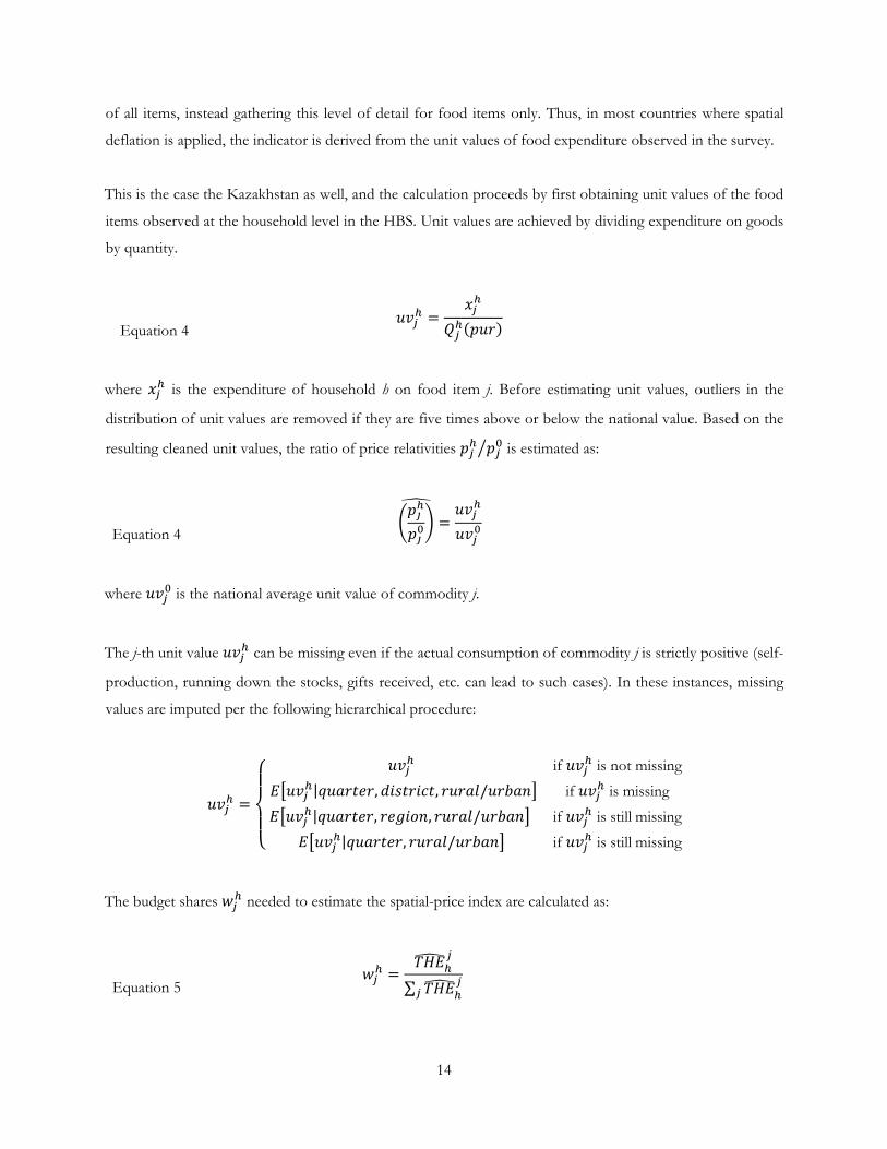
of all items, instead gathering this level of detail for food items only. Thus, in most countries where spatial
deflation is applied, the indicator is derived from the unit values of food expenditure observed in the survey.
This is the case the Kazakhstan as well, and the calculation proceeds by first obtaining unit values of the food
items observed at the household level in the HBS. Unit values are achieved by dividing expenditure on goods
by quantity.
Equation 4
where is the expenditure of household h on food item j. Before estimating unit values, outliers in the
distribution of unit values are removed if they are five times above or below the national value. Based on the
resulting cleaned unit values, the ratio of price relativities is estimated as:
Equation 4
where is the national average unit value of commodity j.
The j-th unit value can be missing even if the actual consumption of commodity j is strictly positive (self-
production, running down the stocks, gifts received, etc. can lead to such cases). In these instances, missing
values are imputed per the following hierarchical procedure:
if is not missing
| , , / if is missing
| , , /
| , /
if is stillmissing
if is stillmissing
The budget shares needed to estimate the spatial-price index are calculated as:
Equation 5 ∑

15
where ∑ is the total household expenditure on all food items j included in the index. The index is first
averaged for each quarter, region, and area combination, and then normalized for each stratum by the national
average.
Equation 6
|
3.2 The Cost of Food
Applying this method to reported food consumption for 2015 in the HBS of Kazakhstan and comparing to the
national average yields the percentage values reported in Figure (4). The index approach reveals that the largest
spatial differences in food costs are between predominantly rural regions and predominantly urban ones. For
instance, the rural and largely agricultural regions of South Kazakstan, Atyrau, West Kazakhstan, Aktobe,
Kostanay, Jambyl, and North Kazakhstan all enjoy lower than average food prices. In these regions, even urban
food prices are lower than the national average. However, the largely urban regions of Astana and Almaty city,
alongside the oil-producing region of Mangystau all have above average prices. The most remarkable differences
arise when comparing Almaty and Astana to the rest of the country. Within-region food costs vary by no more
than about 5 percent in most cases, and are not substantially different by rural and urban areas.
Figure 4: Rural vs. Urban Food-based Spatial Deflation Index
Source: The Household Budget Survey of Kazakhstan, Author’s Calculations. Note: Values are expressed in terms of a percentage of the national average.
85.0%
90.0%
95.0%
100.0%
105.0%
110.0%
115.0%
Urban Rural

16
Although food prices in Kazakhstan are higher in urban areas than in rural areas, this is the case in most
countries. Kazakhstan is an exception only in degree. With a maximum of 115 percent of the national average,
and a minimum of about 90 percent of the national average, Kazakhstan records some of the largest average
differences between urban and rural prices in Europe and Central Asia (ECA). Food in the two largest cities of
Astana and Almaty is between 7 and 15 percent more expensive than the national average, and the cost of food
in Almaty is on average more than 28 percent higher than the least expensive region (in 2015, rural areas in the
South Kazakhstan region). This difference likely partially reflects differences in quality, but is also strongly
associated with the economic development of the region. Figure (5) provides maps of the index value and a
clustering analysis that highlights regions of high vs. low average food prices. The results highlight important
spatial concentrations of higher food prices in the country. In general, urban areas are more expensive than
rural areas on this measure; however, prices are also substantially higher in the east, and lower in the western
part of the country.
Figure 5: Food Index Value by District (left), Food Index Hot-Cold Spots (right)
Source: The Household Budget Survey of Kazakhstan, Author’s Calculations.
In Kazakhstan, households in the bottom quintile allocated about 69 percent of their total budget to food in
2015, much more than the 48 percent allocated to food by the top quintile over the same period. High food
prices reduce the disposable income of (non-producer) households, and are particularly problematic for the
poor.

17
Standard poverty estimates in Kazakhstan12 partially account for the spatial differences in the cost of food.
Thus, one method of highlighting the role that regional price differences play in poverty and economic well-
being is to compare poverty rates using spatially adjusted and non-adjusted consumption. The results of this
comparison are reported in Figure (6). Ignoring the standard spatial adjustments for Kazakhstan13 would result
in a poverty rate nearly 12 percent higher in South Kazakhstan, 9 percent higher in Atyrau, and 5 percent higher
in each of the three regions of Kostanay, West Kazkahstan, and Kyzylorda. These regions are predominantly
rural, and the low food prices prevalent in those regions help to reduce the poverty rate. However, this
comparison also implies that more than 421,000 people (about 2.4 percent of the population) would fall below
the poverty line if they moved to an area where food prices coincided with the national average (while
maintaining the same budget).
Figure 6: Poverty Rates at $5-a-day 2005 PPP with and without Spatial Food Price Deflation (left)
3.3 The Cost of Housing
Housing costs can be analyzed in the same index framework by including imputed rent as a component of the
Paache index. Including the cost of rent into Equation 1 as an additional consumption item proceeds by
assuming the “quantity” of rent is one (i.e., that the household pays imputed rent on only a single dwelling) and
12 In this case, using the international poverty line at $5-a-day in 2005 PPP, and a welfare aggregate that excludes imputed rent. 13 Based on a strata-level measure and the unit values of food consumption.
0%
5%
10%
15%
20%
25%
30%
35%
40%
45%
Without Spatial Deflation With Spatial Deflation

18
including the resulting unit value as a separate expenditure item for the household. This is conceptually different
from most reported food expenditure in the sense that although something of value was consumed (use of the
dwelling) no financial transaction took place.
The values reported in Table (5) are disaggregated to explore two alternative measures of imputed rent in this
framework. The first uses imputed rent directly as reported in the HBS. This method implicitly assumes that
housing is the same “good” for all consumers, regardless of the type of dwelling, and compares the overall
differences in the resulting cost-of-living as a partial function of the unmodified imputed housing cost. A
second alternative is to use a hedonic housing price measure. The second approach is more common in the
literature on measuring the cost-of-living, and imposes the requirement that the spatial deflator for housing be
based on consumption of a similar “type” of housing, in terms of size and construction. In both cases, the
housing costs are included alongside the other components of the Paache index.
There is no estimation for the first option, as self-reported values are included directly. However, the hedonic
option is implemented using a separate imputation technique. The process proceeds by imputing the cost of
renting the same “standard” dwelling in each locality, and including this value in the overall cost-of-living index.
The first step involves estimating a simple ordinary least squares (OLS) regression of reported rental values:
… …
Where is reported rental value of the home, and the term includes housing characteristics of interest,
including dummy variables indicating location. Based on the resulting coefficients, a predicted rental value by
locality is generated by holding constant a set of housing characteristics. Included in the application described
here were variables for the living space of the dwelling (assumed to be 42 M Sq. for “standard” housing), the
number of rooms (assumed to be 3 for “standard” housing), a dummy variable for whether the location is rural
or urban, and the type of dwelling (assumed to be an apartment for “standard” housing). The results of the
estimation procedure were then included as a component of the price index described above (instead of
imputed rent for the housing that households report having consumed).

19
Table 5: Estimated Food-based, Food + Rent-based, and Food + Standard Rent-based Indexes by
Region and by Rural and Urban areas (National Average = 100%)
All Urban Rural
Food Only
Food + Imp Rent
Food + Standard Rent
Food Only
Food + Imp Rent
Food + Hedonic Rent
Food Only
Food + Imp Rent
Food + Hedonic Rent
Akmola 99% 88% 67% 97% 112% 109% 101% 69% 62% Aktobe 95% 103% 79% 97% 159% 121% 94% 90% 78% Almaty 105% 94% 77% 106% 124% 117% 104% 92% 74% Atyrau 93% 94% 112% 93% 157% 116% 91% 73% 77% West Kaz 93% 75% 73% 94% 154% 116% 91% 71% 71% Jambyl 97% 90% 64% 97% 131% 105% 97% 77% 61% Karaganda 99% 114% 101% 99% 133% 102% 98% 70% 56% Kostanay 94% 71% 56% 95% 138% 99% 94% 48% 51% Kyzylorda 96% 71% 64% 98% 133% 102% 95% 61% 61% Mangystau 103% 150% 157% 103% 274% 167% 101% 105% 123% South Kaz 91% 86% 56% 92% 128% 96% 90% 67% 53% Pavlodar 101% 99% 71% 101% 143% 113% 100% 94% 68% North Kaz 98% 72% 62% 98% 147% 108% 98% 55% 59% East Kaz 104% 82% 68% 103% 121% 108% 104% 62% 60% Astana city 107% 304% 240% 107% 304% 240% . . Almaty city 115% 253% 190% 115% 253% 190% . .
Source: The Household Budget Survey of Kazakhstan, Author’s Calculations. Note: provides a comparison of average imputed rent (left) with hedonic rent estimate (right). Appendix (B) includes the OLS regression model and coefficients used for the imputation procedure.
For both methods the estimated differences in the cost of housing are much larger than the cost of food
described in the previous section. In 2015, imputed rent was on average three times higher in urban areas than
in rural areas (540,000 vs. 180,000 Tenge per year).14 Imputed rent in regions with the lowest average costs
(including Kostanay, Kyzylorda and North Kazakhstan) was only 15 percent of the imputed rent in the highest
cost area (Astana City). Table (5) reports several cost-of-living indices across regions and rural and urban areas.
Including imputed rent costs highlights large and economically significant differences in the cost-of-living, both
within and between regions. The overall national trend is for a substantially higher cost-of-living in urban areas
after accounting for imputed rental costs, and particularly for the two largest cities of Almaty and Astana.
Pricing a standard apartment in each region using a hedonic model instead of reported imputed rent moderates
the disparity to some extent (reducing the difference in the cost-of-living from 304 percent to 240 percent
above the national average in Astana city, and from 253 percent to 190 percent in Almaty), but the magnitudes
14 Please see appendix F for average imputed rental values and hedonic rent estimates for housing by region.

20
remain large. Due to the much lower than average cost of housing in the most rural areas, using the hedonic
approach rather than the unadjusted imputed rent approach further improves the cost-of-living in these areas
relative to the national average (for example, see Kostanay and South Kazakhstan in Table (5)). After including
imputed rent in the index, not a single urban area is estimated to have lower cost-of-living than the national
average. In contrast, rural areas are all well below the national average with the sole exception of Mangystau.
Figure 7: Index of Imputed Rent (left), Hot-Cold Spot Map of Imputed Rent (right)
Source: The Household Budget Survey of Kazakhstan, Author’s Calculations.
Figure (7) maps the values of the index of imputed rental costs, and a spatial analysis of clustering of very high
or very low costs. The results highlight the large disparity in the cost of housing for rural vs. urban areas, and
particularly for the cities of Astana and Almaty. The areas surrounding the two largest cities are also identified
as “hot-spots” where prices are substantially higher, whereas the north-central part of the country is noted for
particularly low housing costs.
4. Affordability
There are several customary approaches to measure the affordability of housing. The HBS data for Kazakhstan
are sufficient for two of the most common: one based on monthly expenditure, and another based on the
estimated value of an occupied dwelling.
Most monthly expenditure approaches of the first type were initially calibrated on data from the United States.
The first such definition was applied in the 1920s and set at monthly expenditure at 25 percent of income (see
Pelletiere (2008) for a detailed history). In later years, the threshold rose to 30 percent of income, which remains
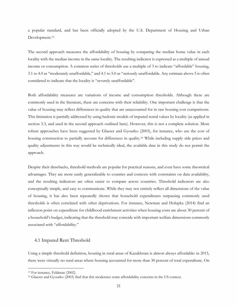
21
a popular standard, and has been officially adopted by the U.S. Department of Housing and Urban
Development.15
The second approach measures the affordability of housing by comparing the median home value in each
locality with the median income in the same locality. The resulting indicator is expressed as a multiple of annual
income or consumption. A common series of thresholds use a multiple of 3 to indicate “affordable” housing,
3.1 to 4.0 as “moderately unaffordable,” and 4.1 to 5.0 as “seriously unaffordable. Any estimate above 5 is often
considered to indicate that the locality is “severely unaffordable”.
Both affordability measures are variations of income and consumption thresholds. Although these are
commonly used in the literature, there are concerns with their reliability. One important challenge is that the
value of housing may reflect differences in quality that are unaccounted for in raw housing cost comparisons.
This limitation is partially addressed by using hedonic models of imputed rental values by locality (as applied in
section 3.3, and used in the second approach outlined here). However, this is not a complete solution. More
robust approaches have been suggested by Glaeser and Gyourko (2003), for instance, who use the cost of
housing construction to partially account for differences in quality.16 While including supply side prices and
quality adjustments in this way would be technically ideal, the available data in this study do not permit the
approach.
Despite their drawbacks, threshold methods are popular for practical reasons, and even have some theoretical
advantages. They are more easily generalizable to counties and contexts with constraints on data availability,
and the resulting indicators are often easier to compare across countries. Threshold indicators are also
conceptually simple, and easy to communicate. While they may not entirely reflect all dimensions of the value
of housing, it has also been repeatedly shown that household expenditures surpassing commonly used
thresholds is often correlated with other deprivations. For instance, Newman and Holupka (2014) find an
inflexion point on expenditure for childhood enrichment activities when housing costs are about 30 percent of
a household’s budget, indicating that the threshold may coincide with important welfare dimensions commonly
associated with “affordability.”
4.1 Imputed Rent Threshold
Using a simple threshold definition, housing in rural areas of Kazakhstan is almost always affordable: in 2015,
there were virtually no rural areas where housing accounted for more than 30 percent of total expenditure. On
15 For instance, Feldman (2002). 16 Glaeser and Gyourko (2003) find that this moderates some affordability concerns in the US context.

22
average, housing accounted for only about 11 percent of total consumption in rural Kazakhstan, and even less
in the most rural parts of the country including Jambyl and Kyzlorda. In contrast, imputed rent in 2015
accounted for more than 28 percent of consumption in urban areas on average. More than 36 percent of urban
households allocated more than 30 percent of their budget to housing in 2015. In the most expensive urban
markets of Astana and the city of Almaty, rent accounted for 36 and 44 percent of total average consumption
respectively in 2015. More than 66 percent and 77 percent of households in Astana and the city of Almaty live
in unaffordable housing, despite enjoying the highest average incomes in the country.
Figure 8: Imputed Rent Share of Total Consumption, 201517
4.2 Home Value Threshold
Measuring the affordability of housing using home values yields qualitatively similar results to the imputed rent
approach. Comparing the median home value with the median income in each locality in 2015 identifies the
same urban centers as the least affordable, while most rural areas were affordable for the large majority of
residents. According to the home values measure, the regions of Akmola, North Kazakhstan, Kyzylorda,
Aktobe, Kostanay, Atyrau, and South Kazakhstan were all “affordable” in 2015 (with a multiple of 3 or less).
In contrast, West Kazakhstan, East Kazakhstan, and Jambyl were all moderately unaffordable (with a multiple
of between 3.1 to 4.0), while Pavlodar, Almaty region, and Karaganda were all severely unaffordable (with
multiples of 4.1 to 5.0).
17 Total consumption per capita is used for the measures adopted here.
0%
10%
20%
30%
40%
50%
60%
70%
80%
90%
100%
Akm
ola
Aktobe
Alm
aty
Atyrau
West Kaz
Jambyl
Karagan
da
Kostan
ay
Kyzylorda
Man
gystau
South Kaz
Pavlodar
North Kaz
East Kaz
Astan
a city
Alm
aty city
All Rural
All Urban
0‐10% 11‐20% 21‐30%
31‐40% 41‐50% 51% and Above
0%
10%
20%
30%
40%
50%
60%
70%
80%
All Rural
Kyzylorda
South Kaz
Alm
aty
North Kaz
Akm
ola
East Kaz
Jambyl
Kostan
ay
Atyrau
West Kaz
Pavlodar
Aktobe
Karagan
da
All Urban
Man
gystau
Alm
aty city
Astan
a city
Average Rent Share Share Above 30

23
At the extreme, Mangystau was above the “severely unaffordable” threshold with a multiple of about 6.2, while
Almaty City and Astana City were both more than twice the threshold, with multiples of 10.6 and 11.8
respectively. The three areas where housing is least affordable are also, in the same order, the regions of the
country that recorded the lowest rates of poverty in 2015 (at 8.9, 7.9, and 5.9 respectively).18 Per the home value
based measure, the cities of Almaty and Astana are more unaffordable than many famously exclusive metro
areas, such as San Francisco in the United States and Vancouver in Canada (Table 6).
Table 6: Kazakhstan Cities Median Multiple Affordability Measures vs. International Cities
Affordability Rank Country City Median Multiple 1 China Hong Kong 18.1 2 Australia Sydney, NSW 12.2
Kazakhstan Astana City 11.8 3 Canada Vancouver, BC 11.8
Kazakhstan Almaty City 10.6 4 N.Z. Auckland 10 5 U.S. San Jose, CA 9.6 6 Australia Melbourne, VIC 9.5 7 U.S. Honolulu, HI 9.4 8 U.S. Los Angeles, CA 9.3 9 U.S. San Francisco, CA 9.2 10 U.K. Bournemouth & Dorset 8.9
Source: 13th Annual Demographia International Housing Affordability Survey: 2017 and The Household Budget Survey of Kazakhstan, Author’s Calculations.
4.3 Simulating Migration Affordability
Another approach to gauging potential housing demand is to simulate a scenario in which a household in a
rural area moves to an urban area. If we assume that in such a scenario, households would pay the median
monthly cost of urban housing following their move, we can estimate the likely budget share of housing in an
urban area for previously rural households. The results of this exercise are presented graphically in Figure (9).
On average, if rural households relocated to the median urban area, they would be expected to spend nearly 20
percent more of their current total budget on housing alone, even before taking differences in the cost of other
goods and services into account. In about half of Kazakhstan’s regions, this would equate to more than
doubling of the share of consumption allocated to housing. In every region other than Mangystau and the cities
18 The middle class, defined as households consuming above the line of $10-a-day in 2005 PPP terms (but excluding imputed rent), was also largest in Astana (34 percent) and Almaty (50.5 percent).

24
of Almaty and Astana, the average imputed rent share would be higher than the 30 percent affordability
threshold applied in section 3.4. The regions of North Kazkahstan and Kostanay do very poorly by this
measure: such a migration in these areas would equate to households spending more than half of their current
total budget, on average. Similar comparisons based on average income are included in Appendix D.
Figure 9: Budget Share Allocated to Rent vs. Simulated Share using Average Urban Rent (left),
Mapping of Simulated Rent Share using Average Urban Rent (right)
One weakness of this approach is that it does not consider the higher incomes prevalent in urban areas. If
households were to relocate, one would expect higher incomes to compensate for a portion of the increase in
the cost-of-living. But although average income in Almaty was 66 percent higher than the national average (and
92 percent higher average in Astana), the price indexes calculated in section 3.3 suggest that the cost-of-living
was 240 percent higher in Astana and 190 percent higher in Almaty. Thus, despite the higher expected income
households could gain from migrating, the high cost-of-living in urban areas would more than overwhelm the
expected monetary benefit for most rural households.
5. Housing Demand Elasticities
5.1 Income and Prices
Accurate measures of the elasticity of housing demand to income and price effects are essential to forecast
trends in urbanization and to formulate related policies. There are also important distributional implications of
demand elasticities. Demand for housing usually rises with income, and in Kazakhstan, following more than a
decade of real average income growth, greater demand for housing is a natural expectation. On the other hand,
0.0%
10.0%
20.0%
30.0%
40.0%
50.0%
60.0%
Astan
a_city
Alm
aty_city
Man
gystau
Atyrau
Alm
aty
Aktobe
Kyzylorda
South_K
az
Pavlodar
Karagan
da
West_K
az
East_K
az
Jambyl
Akm
ola
North_K
az
Kostan
ay
Rent Share Assuming Urban Average

25
housing’s status as a necessity good means that one would expect housing demand to be relatively inelastic to
price and income. Although poor people are often especially sensitive to price changes, if housing demand is
on average inelastic to price, as prices rise the poor may become more budget constrained rather than consume
less housing, and housing would effectively displace other consumption. Conversely, if households are relatively
responsive to price, they may be reluctant to move to areas experiencing rapid price appreciation, or more likely
to move away in favor of lower cost areas. This latter scenario is of greatest interest with regards to the future
of urbanization in Kazakhstan, as prices have risen much more quickly than incomes in urban areas over the
past decade.
Depending on market trends, price and income effects can work either in tandem or in opposite directions.
However, it is common for incomes to rise while housing prices increase (and vice versa), as has been the case
in Kazakhstan over the past decade. Thus, with respect to the net change in demand due to these factors, either
the income or the price effect could dominate. The analysis described in this section provides demand elasticity
estimates for both income and price, and show that demand in Kazakhstan is quite responsive to changes in
both income and price in comparison to other countries. However, the absolute value of the elasticity to price
is larger, even as prices have risen faster than have incomes, suggesting that rising prices have reduced demand
for housing in high-cost localities on net, and in turn, discouraged urbanization.
5.2 Estimation
Using imputed rent, cross-sectional demand elasticities can be estimated using a standard utility maximization
approach:19
Equation 7 ,
Where a household’s utility ( ) is a function of the consumption of housing ( ) and other goods ( ).
Households maximize utility subject to a budget constraint.
Equation 8
The term is total income (here, approximated in the following using total consumption, is the unit price
of housing, and is a price index for all non-housing goods. Maximization yields a demand function for
housing:
19 The description here draws from the approach outlined in Grootaert and Dubois (1988).

26
Equation 9 ,
In the case of housing, such a model is difficult to evaluate empirically because only consumption of housing
is observed (either as the home value, or in the form of imputed rent). The solution applied in much of the
literature is to consider imputed rent as a dependent variable and to decompose rent into price and quantity
components (see Malpezzi (1999); Grootaert and Dubois (1988); and Follain et al. (1980) for examples). This
approach is adopted here using the hedonic rent value calculated as per the procedure described in section 3.1
as the price variable. The estimation proceeds using a log-log method to estimate the elasticities associated with
each term, such that:
Equation 10 ln ln 1 ln
Where the term is the log of imputed rent, ln is the log of household income, ln is the log price
of housing from the hedonic regression. The elasticity associated with household income is the term , while
1 yields the demand elasticity to price.
5.3 Elasticity and Comparisons
The results of the estimation are reported in Table (7).20 The findings suggest an elasticity of demand to total
consumption (a proxy for permanent income) of between .54 and .61 for rural and urban areas separately,
and .66 for the population overall. Put differently, a 10 percent increase in income is associated with a 5.4
percent increase in housing consumption for rural housing, 6.1 percent increase for urban housing, and a 6.6
percent increase nationally. By way of comparison, Malpezzi and Mayo (1985) provide income elasticities across
eight countries with a range of between 0.4 to 0.6. Malpezzi (1999) also reports income elasticities across many
studies falling within this range. The national estimate for Kazakhstan is thus roughly at the upper end of the
standard range found in the literature.21
20 Note that the signs for the coefficients are in the expected direction, and the models have relatively goodness of fit, as measured by the . 21 Though other studies of specific markets have found higher estimates.
27
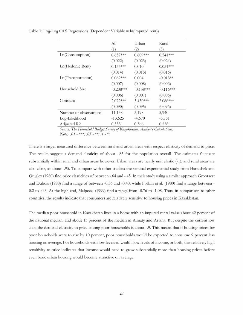
Table 7: Log-Log OLS Regressions (Dependent Variable = ln(imputed rent))
All Urban Rural (1) (2) (3) Ln(Consumption) 0.657*** 0.609*** 0.541***
(0.022) (0.023) (0.024) Ln(Hedonic Rent) 0.155*** 0.010 0.051***
(0.014) (0.015) (0.016) Ln(Transportation) 0.062*** 0.004 -0.013**
(0.007) (0.008) (0.006) Household Size -0.208*** -0.158*** -0.116***
(0.006) (0.007) (0.006) Constant 2.072*** 3.430*** 2.086*** (0.090) (0.095) (0.096) Number of observations 11,138 5,198 5,940 Log-Likelihood -13,625 -4,670 -5,751 Adjusted R2 0.333 0.366 0.258 Source: The Household Budget Survey of Kazakhstan, Author’s Calculations. Note: .01 - ***; .05 - **; .1 - *;
There is a larger measured difference between rural and urban areas with respect elasticity of demand to price.
The results suggest a demand elasticity of about -.85 for the population overall. The estimates fluctuate
substantially within rural and urban areas however. Urban areas are nearly unit elastic (-1), and rural areas are
also close, at about -.95. To compare with other studies: the seminal experimental study from Hanushek and
Quigley (1980) find price elasticities of between -.64 and -.45. In their study using a similar approach Grootaert
and Dubois (1988) find a range of between -0.36 and -0.40, while Follain et al. (1980) find a range between -
0.2 to -0.3. At the high end, Malpezzi (1999) find a range from -0.76 to -1.08. Thus, in comparison to other
countries, the results indicate that consumers are relatively sensitive to housing prices in Kazakhstan.
The median poor household in Kazakhstan lives in a home with an imputed rental value about 42 percent of
the national median, and about 13 percent of the median in Almaty and Astana. But despite the current low
cost, the demand elasticity to price among poor households is about -.9. This means that if housing prices for
poor households were to rise by 10 percent, poor households would be expected to consume 9 percent less
housing on average. For households with low levels of wealth, low levels of income, or both, this relatively high
sensitivity to price indicates that income would need to grow substantially more than housing prices before
even basic urban housing would become attractive on average.

28
Figure 10: Growth Incidence Curve for 2006-2015 (Left), Approximation of Engel Curve for Imputed
Rent and Total Consumption (Right)
Source: The Household Budget Survey of Kazakhstan, Author’s Calculations.
Because price elasticities are higher than income elasticities in absolute terms, price has a greater influence on
housing consumption than does household income for a given percentage change. Figure (10) provides the
growth incidence curve for consumption. Although growth has been pro-poor in recent years, the average
annual growth rate in housing costs between 2001 and 2016 was about 16 percent, well above even the highest
performing quantiles. Because the price effect is expected to dominate the income effect, demand is likely being
strongly restrained by these high prices, and is consistent with the slow rate of urbanization in Kazakhstan.
6. Mobility, Ownership, and the Rental Market
There is a strong consensus in the literature that homeowners are less geographically mobile than renters.
Hughes and McCormick (1985) provide some of the first empirical demonstrations that housing policy
significantly reduces mobility, while also noting that the findings are consistent with the literature dating from
the late 1960s. More recent studies have repeatedly confirmed that homeowners are less mobile (see, for
instance, Barcelo, 2006; Andrews and Sánchez, 2011). This empirical regularity is of crucial importance in
Kazakhstan, where outside a small market in Astana, nearly all households own their dwelling.
The absence of affordable rental options is a crucial missing step in the urbanization ladder, and low-income
people are especially likely to be affected by high rates of home ownership. In the absence of a rental market,
low-income people are not able to move to high cost areas, as they are usually unable to purchase housing in
high cost locations. Acquiring new housing is usually “front-loaded,” in the sense that purchasing a dwelling
29
usually requires a large up-front payment. For most rural households, this one-time cost is unachievable given
their income and equity in lower-cost rural housing. Such costs are unrealistic for most rural households in a
context where house prices are rising by 50 percent per year or more, and cost upwards of 11 times the annual
total household consumption of even relatively well-off urban residents. This relationship ultimately restricts
the population of rural residents with the financial ability to relocate to urban areas, despite the other public
and private benefits to doing so.22
6.1 The Soviet Legacy
High home ownership rates in Kazakhstan are largely a legacy of the Soviet Union’s housing policies (Struyk,
2000). The widespread housing privatization efforts undertaken in most CIS countries and among formerly
managed economies in Eastern and Central Europe led to much higher rates of home ownership in these areas
than in Western Europe. Among the EU member states that were formerly part of the Soviet Union, none has
a rental market share that is above the EU average.23
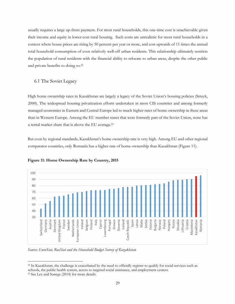
But even by regional standards, Kazakhstan’s home ownership rate is very high. Among EU and other regional
comparator countries, only Romania has a higher rate of home ownership than Kazakhstan (Figure 11).
Figure 11: Home Ownership Rate by Country, 2015
Source: EuroStat, RusStat and the Household Budget Survey of Kazakhstan
22 In Kazakhstan, the challenge is exacerbated by the need to officially register to qualify for social services such as schools, the public health system, access to targeted social assistance, and employment centers. 23 See Lex and Sunega (2014) for more details.
30
40
50
60
70
80
90
100
Switzerlan
d
German
y
Austria
Den
mark
United
Kingd
om
Fran
ce
Swed
en
Netherlands
European Union
Irelan
d
Belgium
Finland
Italy
Cyp
rus
Luxembourg
Portugal
Greece
Slovenia
Icelan
d
Czech Rep
ublic
Spain
Latvia
Malta
Serbia
Estonia
Bulgaria
Norw
ay
Poland
Hungary
Russia
Slovakia
Lithuan
ia
Croatia
Maced
onia
Kazakhstan
Roman
ia

30
In addition to the drive for privatization following independence, policy-related impediments may also play a
role in explaining the high share of households that own their homes. Hughes and McCormick (1981) note that
UK housing policies lead to “extreme shortages of rental accommodation in certain areas.” Similarly,
Gilderbloom and Appelbaum (1987) argue that housing policies and other market imperfections have led to
shortages in affordable rental units throughout the United States.
Privatizing government-owned housing in the wake of the breakup of the Soviet Union provided significant
benefits for most recipient households, and in some countries, subsides were moderately pro-poor (Struyk,
2000). Under privatization, sitting tenants had the right to purchase their units, typically at a substantial discount
or, in some cases, for free except for a nominal processing fee. Take-up of such privatization offers was very
high. Due in part to the appreciation in home values that followed in many CIS countries, a popular view
emerged that, in comparison to alternative investments or the banking system, housing was a preferable means
of storing wealth. Even though privatizations were ultimately very costly to the governments involved, the
programs were extremely popular throughout the former Soviet Union (Struyk, 2000). Home ownership has
also been shown to be positively associated with better education outcomes for children (Haurin et al. 2002)
and higher levels of community engagement (Di Pasquale and Glaeser, 1999).
6.2 The Labor Market
But despite the clear beneficial aspects of home ownership, there are significant drawbacks as well. In a seminal
study using cross-country comparisons of unemployment, Oswald (1996) finds that by reducing mobility, a
high rate of home ownership directly impedes the functioning of the labor market. Dohmen (2004) develops a
related theoretical model to show that the high moving costs related to home ownership are a severe
impediment to regional mobility, which is hypothesized to ultimately lead to dysfunction in labor markets. In
addition, the model suggests that higher moving costs reduce on-the-job search effort and effectiveness, which
in turn would be expected to reduce potential productivity.
Supplementing the view articulated in Oswald (1996) and related work, Blanchflower and Oswald (2013) find
that increasing home-ownership rates are a precursor to rising unemployment, and suggest that lower worker
mobility is primarily to blame.24 The results suggest that the impact of high ownership rates on the labor market
are significant at the macro level: a doubling of the rate of home-ownership can be followed in the long-run by
more than a doubling of the unemployment rate.
24 Secondary issues include greater commuting times and fewer new businesses in areas with high ownership rates.

31
Although not universal,25 the negative relationship between home ownership and the functioning of the labor
market has since been replicated in many other settings. Munch et al. (2008) find that home ownership in
Denmark has a negative impact on job-to-job mobility both in terms of transition into new local jobs and new
jobs outside the local labor market. In a study focusing on the UK, Battu et al (2008) find much the same
relationship. Laamanen (2017) also finds that home-ownership has a significant and causal effect on
unemployment.26 In each of these studies, the negative effect on labor markets is primarily driven by reduced
worker mobility.27
Figure 12: The Share of Owner-Occupied Out of Total Occupied Housing by Region in 2015
Source: The Household Budget Survey of Kazakhstan, Author’s calculations
The movement of workers from low-productivity rural areas to high productivity urban ones has also
traditionally been one of the primary drivers of regional economic convergence. Models of wage rate
convergence, such as that proposed by Ganong and Shoag (2017), begin with the proposition that wage premia
in higher productivity geographic areas attract qualified workers. Over time, this process leads to an increasing
supply of labor in areas with above average wages, while reducing the supply of labor in lower productivity
25 Many studies show that homeowners are less likely to be unemployed than renters. For instance, Van Leuvensteijn and Koning (2004) demonstrate that this is the case in the Netherlands. 26 Laamanen (2017) also finds that homeowners are less likely to be unemployed than non-owners, providing an explanation for the apparent inconsistency between Oswald (1996) and the empirical results from Van Leuvensteijn and Koning (2004), among others. 27 Laamanen (2017) also highlights the role of policy in the rental market: the deregulation used for the identification strategy was shown to substantially increase the supply of rental dwellings on the market by making renting more profitable for landlords.
0%
10%
20%
30%
40%
50%
60%
70%
80%
90%
100%
Own Other

32
areas. With more workers to choose from, employers would be expected to negotiate wages more aggressively
in high productivity areas, while workers who remain in lower productivity locations would face less
competition from other workers, and negotiate for higher wages. Unhindered, most theoretical models suggest
that this process would be expected to continue until wages roughly equalize across regions. The relationship
has been empirically validated in many contexts. In the case of the United States, regional convergence between
1880 and 1980 continued at a stable rate of about 1.8 percent per year. However, Ganong and Shoag (2017)
show that the rising cost of housing in cities beginning in 1980 led to 50 percent slowdown in the rate of
regional wage convergence. Absent these impediments to mobility, the authors estimate that wage inequality
would have been 8 percent smaller between 1980 and 2010.
Recently, a similar pattern is apparent in urban Kazakhstan, with the noted exception of Astana. The two most
economically dynamic urban centers of Astana and Almaty enjoy higher wages than the rest of the country
(even after controlling for gender, sector, and level of education). But while convergence has rapidly continued
in Astana, where the rental market is largest, convergence largely halted in Almaty and other urban areas in
2011. While it is unlikely that these trends are entirely driven by the rental market and the cost of housing, they
are consistent with the experiences of other upper-middle income countries, as well as the best-studied
international examples, such as the United States. Figure (13) reports the wage differentials between 2006 and
2015 in more detail.
Figure 13: Location-Specific Wage Residual (National Average=0%)
Source: The Household Budget Survey of Kazakhstan, Author’s calculations
‐30%
‐20%
‐10%
0%
10%
20%
30%
40%
2006 2007 2008 2009 2010 2011 2012 2013 2014 2015
Almaty Astana All Rural All Urban

33
6.3 Macroeconomic Effects
These effects can be sufficient to translate to large effects on aggregate economic performance. Hsieh & Moretti
(2017) find that spatial misallocation of labor in the US lowered aggregate US growth by more than 50% from
1964 to 2009. Parkhomenko (2017) finds that regulations liming new housing construction accounted for
approximately 23 percent of the wage dispersion, and 85 percent of housing price dispersion in metro areas
between 1980 and 2007 in the US. The analysis also indicated that had regulations not increased over this time,
US output in metro areas would have been 2 percent higher. In most such studies, policies and regulations,
alongside social preferences, are particularly important determinants of the cost of housing (Rubaszeka and
Rubio, 2017).
A small but influential literature makes the case that the absence of a rental housing market may also be a
primary determinant of the business cycle, above and beyond the potential impacts on employment (Czerniak
and Rubaszek, 2016). In an influential paper, Arce and Lopez-Salido (2011) argue that housing bubbles are
caused by homeowners treating their properties as investments, and suggest that the presence of a robust rental
market substantially reduces the risk of a housing bubble and can moderate the economic cycle. This is of
interest in Kazakhstan considering the country’s experience with quickly rising prices between 2001 and 2007.
7. Conclusion
Greater urbanization is an important goal in Kazakhstan’s national development strategy. But the high cost-of-
living in urban areas relative to rural areas in Kazakhstan lowers living standards for urban residents, and inhibits
rural-to-urban migration. The cost of food is substantially higher in urban areas than in rural areas, and the
difference in the cost of housing calculated using imputed rental costs is much larger. The high cost of living
in urban areas alongside the lack of a rental housing market makes the most dynamic labor markets in the
country unaffordable to most low-income households. Simulations conducted in this study find that few rural
households are financially capable of moving to urban areas (even in second tier cities) suggesting a significant
impediment to achieving the government’s urbanization goals.
Constraints to internal migration are a crucial factor for Kazakhstan’s future economic growth. Cities are
commonly the divers of economic growth and diversification in middle-income countries, and without a large
and growing pool of workers located in cities, theory and global experience suggest that businesses will struggle
with the trade-off between the benefits of agglomeration and high labor costs. There is already a large income
gap for jobs in the cities of Almaty and Astana, and to a lesser extent in other urban areas as well. But for the

34
poor and middle class households who may otherwise consider moving to access these opportunities, the cost-
of-living is an important limitation. Providing basic services including water, electricity, education and health
care is substantially more expensive in rural areas, and if a large share of the population in Kazakhstan is priced
out of living in cities and remains in rural areas, they will remain costlier to serve.
These results suggest important policy questions for further exploration. In many of Kazakhstan’s peer
countries, high housing prices tend to reflect constrained supply coupled with high demand, with the latter
often unmet due to regulatory hurdles or other impediments to construction and investment. Access to
transportation is also a common concern for densely populated areas, as congestion can lead to larger premiums
paid for transport-accessible housing in cities, or higher costs for personal modes of transportation. For the
poor and middle class, this can mean accessing more remunerative jobs in cities requires long and costly
commutes from outside urban areas. Supporting the creation and expansion of a rental housing market is a
core recommendation of the latest OECD assessment of the country’s urbanization strategy (OECD, 2017).
Registration requirements such as the propiska system in many former Soviet countries have also contributed
to underperformance in rental markets.
Urban growth commonly leads to poverty reduction and improved access to basic services, and urbanization
in Kazakhstan would very likely contribute to improving standards of living. However, the acute divergence in
the cost-of-living in urban areas relative to the countryside is a threat to Kazakhstan’s growth strategy and will
inhibit the country from achieving key development objectives.

35
Appendix A: Additional Indicator Mapping
Table 8: Comparison of the Observed Share of Imputed Rent in Total Consumption (left) vs.
Simulated Rent using average Urban Imputed Rent (Right)
Table 9: Comparison of Index of Imputed Rent (left) to Index of Dwelling Value (right)

36
Appendix B: Imputed Rent Model for “standard” Apartment
y= Annual Imputed Rent OLS
The living space inhabited by HH 674.454***
(128.827)
How many living rooms inhabited by HH 37,603.448***
(2,676.055)
Dwelling Type 2 -224,705.997***
(41,185.943)
Dwelling Type 3 -126,726.730***
(5,427.233)
Dwelling Type 4 -103,078.839***
(8,034.620)
Urban Area 262,240.176***
(4,856.847)
Constant 176,623.607***
(10,805.581)
Number of observations 11,191
Adjusted R2 0.720
note: .01 - ***; .05 - **; .1 - *; Region Dummies Not Shown

37
Appendix C: Imputed and Hedonic Rent Estimates
Table 10: Average Imputed Rent Paid vs. Average Imputed "Standard" rent in 1000s of Tenge, HBS
2015
Imputed Rent (Reported)
Imputed Rent (Hedonic)
Average
Rent
Average
Urban
Rent
Average
Rural
Rent
Average
Hedonic
Average
Rural
Hedonic
Average
Rural
Hedonic
Akmola 276 411 168
366 506 244
Aktobe 397 490 255
487 587 324
Almaty 272 401 232
349 548 286
Atyrau 358 588 161
441 580 318
West_Kaz 341 525 168
425 559 297
Jambyl 271 399 184
332 489 226
Karaganda 389 448 170
409 463 201
Kostanay 263 432 96 327 453 190
Kyzylorda 259 456 110 319 469 206
Mangystau 687 1032 354
738 872 609
South_Kaz 247 363 153
295 440 178
Pavlodar 364 425 218
451 530 267
North_Kaz 241 420 120
347 498 236
East_Kaz 294 404 141
384 492 230
Astana_city 1266 1266 .
1279 1279 .
Almaty_city 925 925 . 974 974 .
Source: The Household Budget Survey of Kazakhstan, Author’s Calculations.
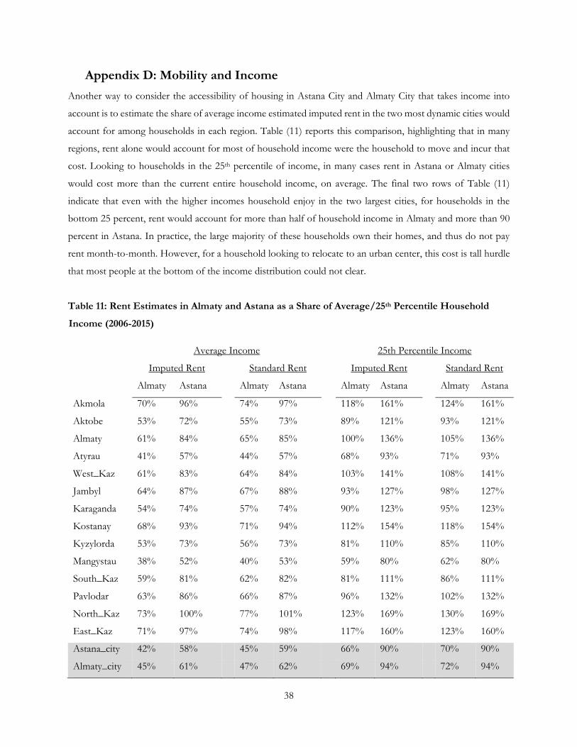
38
Appendix D: Mobility and Income
Another way to consider the accessibility of housing in Astana City and Almaty City that takes income into
account is to estimate the share of average income estimated imputed rent in the two most dynamic cities would
account for among households in each region. Table (11) reports this comparison, highlighting that in many
regions, rent alone would account for most of household income were the household to move and incur that
cost. Looking to households in the 25th percentile of income, in many cases rent in Astana or Almaty cities
would cost more than the current entire household income, on average. The final two rows of Table (11)
indicate that even with the higher incomes household enjoy in the two largest cities, for households in the
bottom 25 percent, rent would account for more than half of household income in Almaty and more than 90
percent in Astana. In practice, the large majority of these households own their homes, and thus do not pay
rent month-to-month. However, for a household looking to relocate to an urban center, this cost is tall hurdle
that most people at the bottom of the income distribution could not clear.
Table 11: Rent Estimates in Almaty and Astana as a Share of Average/25th Percentile Household
Income (2006-2015)
Average Income 25th Percentile Income
Imputed Rent Standard Rent Imputed Rent Standard Rent
Almaty Astana
Almaty Astana
Almaty Astana
Almaty Astana
Akmola 70% 96%
74% 97%
118% 161%
124% 161%
Aktobe 53% 72%
55% 73%
89% 121%
93% 121%
Almaty 61% 84%
65% 85%
100% 136%
105% 136%
Atyrau 41% 57%
44% 57%
68% 93%
71% 93%
West_Kaz 61% 83%
64% 84%
103% 141%
108% 141%
Jambyl 64% 87%
67% 88%
93% 127%
98% 127%
Karaganda 54% 74%
57% 74%
90% 123%
95% 123%
Kostanay 68% 93%
71% 94%
112% 154%
118% 154%
Kyzylorda 53% 73%
56% 73%
81% 110%
85% 110%
Mangystau 38% 52%
40% 53%
59% 80%
62% 80%
South_Kaz 59% 81%
62% 82%
81% 111%
86% 111%
Pavlodar 63% 86%
66% 87%
96% 132%
102% 132%
North_Kaz 73% 100%
77% 101%
123% 169%
130% 169%
East_Kaz 71% 97%
74% 98%
117% 160%
123% 160%
Astana_city 42% 58% 45% 59% 66% 90% 70% 90%
Almaty_city 45% 61% 47% 62% 69% 94% 72% 94%

39
Appendix E: Inequality
Consumption-based inequality estimates for Kazakhstan traditionally do not include imputed rental values.
However, including imputed rent amplifies the measured inequality in the country (Figure 14).
Figure 14: Gini Coefficient by Year
Source: The Household Budget Survey of Kazakhstan, Author’s Calculations.
Without Imputed Rent With Imputed Rent Gini 90/10 90/50 10/50 Gini 90/10 90/50 10/50 2015 0.271 3.184 1.898 0.596 0.292 3.502 2.018 0.576 2014 0.272 3.249 1.892 0.582 0.285 3.502 1.979 0.565 2013 0.262 3.097 1.849 0.597 0.285 3.416 1.987 0.582 2012 0.274 3.321 1.922 0.579 0.294 3.622 2.038 0.563 2011 0.273 3.291 1.920 0.583 0.292 3.547 2.024 0.571 2010 3.287 1.949 0.593 3.460 2.041 0.590 2009 0.278 3.355 1.933 0.576 0.291 3.423 1.966 0.574 2008 0.286 3.352 1.962 0.585 0.325 3.446 2.009 0.583 2007 0.295 3.487 1.953 0.560 0.325 3.564 1.987 0.558 2006 0.299 3.587 1.980 0.552 0.320 3.638 2.005 0.551
0.240
0.250
0.260
0.270
0.280
0.290
0.300
0.310
0.320
0.330
2006 2007 2008 2009 2011 2012 2013 2014 2015
Gini No Imputed Rent Gini With Imputed Rent

Appendix F: Mincer Earnings Function
Dependent Variable = Individual Labor Income 2006 2007 2008 2009 2010 2011 2012 2013 2014 2015
Publicly Owned Entity
24,519* 29,001* 5,977* 21,337* 28,381* . 10,353* -21,379* -25,597* -52,410*
(13,497) (13,879) (21,338) (15,050) (14,787) . (24,044) (34,001) (38,474) (25,767)
Male 94,491*** 120,922*** 137,145*** 135,146*** 155,471*** 163,496*** 198,944*** 226,484*** 270,198*** 285,918*** (15,554) (14,301) (17,511) (16,989) (17,326) (25,273) (27,595) (26,264) (24,529) (33,174)
Age 1,708* 2,244.481* 2,833.062* 3,492.361** 3,432.649** 4,059.306** 4,031.510** 4,348.179** 4,101.551* 3,961.153 (833) (1,170) (1,341) (1,343) (1,330) (1,667) (1,689) (1,966) (2,126) (2,636) Secondary Education
75,937*** 93,695*** 83,678*** 111,163*** 126,883*** 348,810*** 362,093*** 483,590*** 240,373*** 612,737***
(8,488) (12,416) (16,581) (16,571) (10,306) (58,504) (58,065) (37,204) (55,018) (87,403)
Tertiary Education 198,561*** 238,642*** 253,060*** 295,821*** 318,784*** 590,658*** 625,860*** 766,598*** 557,283*** 951,250*** (17,208) (15,975) (20,223) (29,668) (28,262) (73,765) (78,474) (40,132) (46,199) (110,017)
Constant 2,481*** 14,962*** 41,937*** 19,082*** 24,393*** -137,816*** -103,817*** -200,647*** 67,165*** -264,232***
(36,205) (56,261) (60,006) (52,756) (56,380) (28,407) (38,412) (99,493) (142,545) (60,297) Number of observations
20,289 20,302 20,534 83,702 42,480 84,760 83,680 83,993 83,678 82,448
Log-Likelihood -274,280 -279,166 -285,479 -1,171,827 -598,666 -1,203,456 -1,196,671 -1,210,196 -1,209,369 -1,199,242
Adjusted R2 0.145 0.140 0.131 0.129 0.122 0.127 0.131 0.125 0.143 0.138
note: .01 - ***; .05 - **; .1 - *;

References
Andrews, Dan, and Aida Caldera Sánchez. "The evolution of homeownership rates in selected OECD countries: Demographic and public policy influences." OECD Journal: Economic Studies 2011.1 (2011): 1-37. Ahmad, Sohail. "Housing demand and housing policy in urban Bangladesh." Urban Studies 52.4 (2015): 738-755. Albouy, David, Gabriel Ehrlich, and Yingyi Liu. Housing demand, cost-of-living inequality, and the affordability crisis. No. w22816. National Bureau of Economic Research, 2016 Barceló, Cristina. "Housing tenure and labour mobility: A comparison across European countries." (2006). Battu, Harminder, Ada Ma, and Euan Phimister. "Housing tenure, job mobility and unemployment in the UK." The Economic Journal 118.527 (2008): 311-328. Blanchflower, David G., and Andrew J. Oswald. Does high home-ownership impair the labor market?. No. w19079. National Bureau of Economic Research, 2013. Cancho, C., N. Kiso, and P. Corral. “Welfare Impact of Macroeconomic Events: The Case of Georgia and Azerbaijan in the Aftermath of the 2015-16 Currency Devaluations. Manuscript, World Bank, (2016). Chen, Shaohua, and Martin Ravallion. “Absolute poverty measures for the developing world, 1981–2004.” Proceedings of the National Academy of Sciences 104.43 (2007): 16757-16762. Davis, Morris A., and Jonathan Heathcote. "Housing and the business cycle." International Economic Review 46.3 (2005): 751-784 De Leeuw, Frank, and Nkanta F. Ekanem. "The supply of rental housing." The American Economic Review 61.5 (1971): 806-817. Deaton, Angus, and Olivier Dupriez. “Spatial price differences within large countries.” Manuscript, Princeton University, July (2011). DiPasquale, Denise, and Edward L. Glaeser. "Incentives and social capital: Are homeowners better citizens?." Journal of urban Economics 45.2 (1999): 354-384. Follain, James, Gill-Chin Lim, and Bertrand Renaud. "The demand for housing in developing countries: The case of Korea." Journal of Urban Economics 7.3 (1980): 315-336. Feldman, Ron. The Affordable Housing Shortage Considering the Problem, Causes and Solutions. No. 2-02. Federal Reserve Bank of Minneapolis, 2002. Ganong, Peter, and Daniel W. Shoag. Why Has Regional Income Convergence in the US Declined?. No. w23609. National Bureau of Economic Research, 2017. Gilderbloom, John, and Richard P. Appelbaum. Rethinking rental housing. Temple University Press, 1987.
42
Glaeser, Edward L., and Joseph Gyourko. "The impact of building restrictions on housing affordability." (2003). Hanushek, Eric A., and John M. Quigley. "What is the price elasticity of housing demand?." The Review of Economics and Statistics (1980): 449-454. Haurin, Donald R., Toby L. Parcel, and R. Jean Haurin. "Does homeownership affect child outcomes?." Real Estate Economics 30.4 (2002): 635-666. Hsieh, Chang-Tai, and Enrico Moretti. “Housing Constraints and Spatial Misallocation.” Manuscript University of California: Berkley, (2017). Hughes, Gordon A., and Barry McCormick. "Migration Intentions in the UK Which Households Want to Migrate and Which Succeed?." The Economic Journal 95 (1985): 113-123. Laamanen, Jani-Petri. "Home-ownership and the labour market: Evidence from rental housing market deregulation." Labour Economics (2017). Leamer, Edward E. Housing is the business cycle. No. w13428. National Bureau of Economic Research, 2007. Lux, Martin, and Petr Sunega. "Public housing in the post-socialist states of central and eastern Europe: Decline and an open future." Housing Studies29.4 (2014): 501-519. Munch, Jakob Roland, Michael Rosholm, and Michael Svarer. "Home ownership, job duration, and wages." Journal of Urban Economics 63.1 (2008): 130-145. OECD (2017), OECD Urban Policy Reviews: Kazakhstan, OECD Publishing, Paris. http://dx.doi.org/10.1787/9789264268852-en Parkhomenko, Andrii. The Rise of Housing Supply Regulation in the US: Local Causes and Aggregate Implications. mimeo, (2017). Pelletiere, Danilo, Getting to the Heart of Housing's Fundamental Question: How Much Can a Family Afford? A Primer on Housing Affordability Standards in U.S. Housing Policy. Available at SSRN: https://ssrn.com/abstract=1132551 or http://dx.doi.org/10.2139/ssrn.1132551 Priemus, Hugo, and Srna Mandič. "Rental housing in Central and Eastern Europe as no man's land." Journal of Housing and the Built Environment 15.3 (2000): 205-215. Ravallion, Martin, Shaohua Chen, and Prem Sangraula. “New evidence on the urbanization of global poverty.” Population and Development Review 33.4 (2007): 667-701. Roberts, Mark, et al. "Urbanization and development: is Latin America and the Caribbean different from the rest of the world?." (2017). Struyk, Raymond J. "Homeownership and Housing Finance Policy in the Former Soviet Bloc-Costly Populism." (2000). Van Leuvensteijn, Michiel, and Pierre Koning. "The effect of home-ownership on labor mobility in the Netherlands." Journal of Urban Economics 55.3 (2004): 580-596