Policy Research Working Paper 7486

Urbanization and Property RightsYongyang CaiHarris Selod

Jevgenijs Steinbuks

Development Research GroupEnvironment and Energy TeamNovember 2015

WPS7486P

ublic

Dis

clos

ure

Aut

horiz

edP

ublic

Dis

clos

ure

Aut

horiz

edP

ublic

Dis

clos

ure

Aut

horiz

edP

ublic

Dis

clos

ure

Aut

horiz

ed

Produced by the Research Support Team

Abstract

The Policy Research Working Paper Series disseminates the findings of work in progress to encourage the exchange of ideas about development issues. An objective of the series is to get the findings out quickly, even if the presentations are less than fully polished. The papers carry the names of the authors and should be cited accordingly. The findings, interpretations, and conclusions expressed in this paper are entirely those of the authors. They do not necessarily represent the views of the International Bank for Reconstruction and Development/World Bank and its affiliated organizations, or those of the Executive Directors of the World Bank or the governments they represent.

Policy Research Working Paper 7486

This paper is a product of the Environment and Energy Team, Development Research Group. It is part of a larger effort by the World Bank to provide open access to its research and make a contribution to development policy discussions around the world. Policy Research Working Papers are also posted on the Web at http://econ.worldbank.org. The authors may be contacted at hselod@worldbank.org.

Since the industrial revolution, the economic development of Western Europe and North America was characterized by continuous urbanization accompanied by a gradual phasing-in of urban land property rights over time. Today, however, the evidence in many fast urbanizing low-income countries points towards a different trend of “urbanization without formalization”, with potentially adverse effects on long-term economic growth. This paper aims to under-stand the causes and the consequences of this phenomenon, and whether informal city growth could be a transitory or a persistent feature of developing economies. A dynamic stochastic equilibrium model of a representative city is developed, which explicitly accounts for the joint dynamics

of land property rights and urbanization. The calibrated baseline model describes a city that first grows informally, with the growth of individual incomes leading to a phased-in purchase of property rights in subsequent periods. The model demonstrates that land tenure informality does not necessarily vanish in the long term, and the social optimum does not necessarily imply a fully formal city, neither in the transition, nor in the long run. The welfare effects of policies, such as reducing the cost of land tenure formalization, or protecting informal dwellers against evictions are subsequently investigated, throughout the short-term transition and in the long-term stationary state.

Urbanization and Property Rights∗

Yongyang Cai†, Harris Selod‡, and Jevgenijs Steinbuks§

JEL classification: O43, P14, R14

Keywords: agglomeration, economic development, informality, land property rights

∗we are grateful to Gilles Duranton, Remi Jedwab, Kenneth Judd, David Palmer, Gulnaz Shara-futdinova, Anthony Yezer, Yves Zenou and participants to the World Bank/George Washington University 2nd Urbanization and Poverty Reduction Research Conference for useful comments. The views expressed in this paper are those of the authors and do not necessarily reflect those of the world bank, its board of directors or the countries they represent.†Yongyang Cai: Hoover Institution, Stanford University and Becker-Friedman Institute, Univer-

sity of Chicago. Email: yycai@stanford.edu.

‡Harris Selod: Energy and Environment Team, Development Research Group, The World Bank. Email: hselod@worldbank.org.

§Jevgenijs Steinbuks: Energy and Environment Team, Development Research Group, The World Bank. Email: jsteinbuks@worldbank.org.

1 Introduction

Over the past two centuries, the world has witnessed unprecedented changes in the form of mas-

sive population growth, continuous urbanization, and economic development. With the advent

of the Industrial Revolution (1760-1840), countries in Western Europe and North America began

to shift from agrarian towards industrialized societies. This involved migration from rural areas

to cities, which, combined with a decline in urban mortality, caused urban populations to grow

at an unprecedented pace. As a result, urbanization rates began to pick up steadily. The propor-

tion of people residing in cities increased dramatically over that period, starting from a low rate

of approximately one-tenth throughout the Middle Ages and the early modern period (Bairoch

1988) and reaching today 81.5 percent in North America and 73.4 percent in Europe (United

Nations, 2014). Simultaneously, North America and Western Europe experienced unprecedented

economic development as urbanization accompanied a profound structural transformation of

their economies whereby employment in the agricultural sector decreased and a large manufac-

turing sector emerged in cities (Bairoch and Goertz 1986, Michaels et al. 2012). At the same

time, declining transport costs facilitated trade between cities, which further stimulated indus-

trial growth. To the extent that cities also facilitated innovation, in particular through dynamic

knowledge and human capital externalities (Lucas 1988, Romer 1990, Glaeser et al. 1992, Black

and Henderson 1999, Bertinelli and Black 2004), it is fair to say that they acted as engines of

growth (Henderson 2005 and 2010, Quigley 2009). The dynamics of urbanization both stimu-

lated and were accelerated by economic development. Urban population growth contributed to

increase labor productivity (and thus income) thanks to pervasive and significant agglomeration

effects whereby workers become more productive when cities become larger (Duranton, 2014a).

This positive relation is represented on the cross-sectional graph plotting per capita GDP against

the urbanization rate for 189 countries (see Figure 1, Panel A below). In accordance with this

graph, it is roughly estimated that a one percentage point increase in the urbanization rate is

associated with a five point increase in per capita gross domestic product (see Duranton 2014b).

A similar relation emerges when plotting U.N. estimates of per capita production for a cross

section of large cities against the corresponding country’s urbanization rate (see Figure 1, Panel

B below). The latter graph suggests that cities tend to be more productive in countries which

are more urbanized.

Several authors contend that these evolutions in the cities of Western Europe and North America

were made possible by the emergence of institutions conducive to economic growth (North 1990

and 1991, Chong and Calderon 2000), such as financial development (Bondenhorm and Cuberes

2010), the degree of democratization (Henderson and Wang 2007), and property rights (Acemoglu

et al. 2005). Improvement in land property rights, in particular, played a crucial role as it favored

the development of manufacturing activities by lowering transaction costs for the transfer of land

to the emerging industries that were locating in cities and by making investments not only more

secure but also more productive (Knack and Keefer 1995). By stimulating the development of

2

Figure 1: Urbanization, Productivity, and Economic Growth

(a) Urbanization and per capita GDP

Source: World Bank. 189 countries. The urbanization rate on the horizontal axis is the percentage shareof population living in cities in 2012. The vertical axis represents the natural log of GDP per capita in2011 U.S. dollar (reproduced from Duranton, 2014b).

(b) Urbanization and city-level productivity

Source: Global Urban Indicators (1998).

3

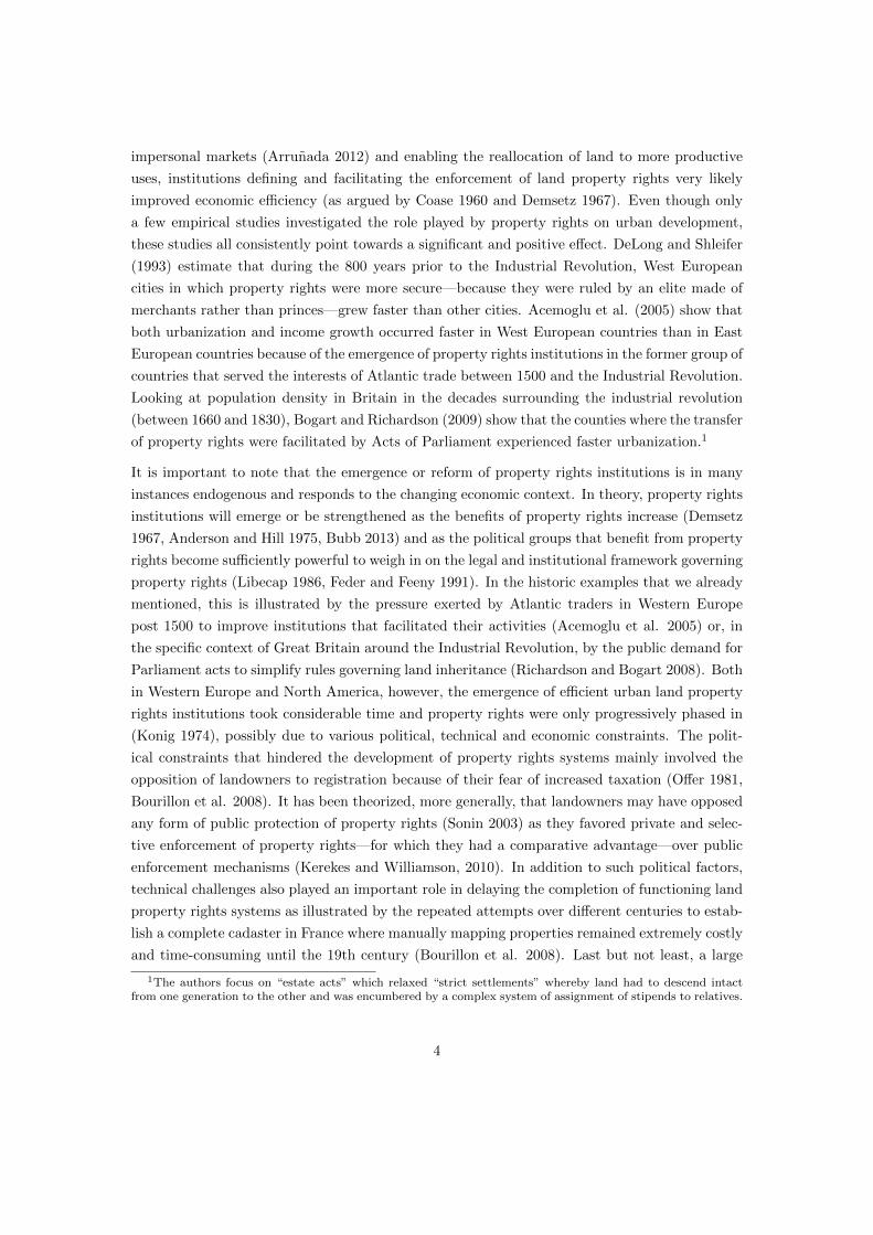
impersonal markets (Arrunada 2012) and enabling the reallocation of land to more productive

uses, institutions defining and facilitating the enforcement of land property rights very likely

improved economic efficiency (as argued by Coase 1960 and Demsetz 1967). Even though only

a few empirical studies investigated the role played by property rights on urban development,

these studies all consistently point towards a significant and positive effect. DeLong and Shleifer

(1993) estimate that during the 800 years prior to the Industrial Revolution, West European

cities in which property rights were more secure—because they were ruled by an elite made of

merchants rather than princes—grew faster than other cities. Acemoglu et al. (2005) show that

both urbanization and income growth occurred faster in West European countries than in East

European countries because of the emergence of property rights institutions in the former group of

countries that served the interests of Atlantic trade between 1500 and the Industrial Revolution.

Looking at population density in Britain in the decades surrounding the industrial revolution

(between 1660 and 1830), Bogart and Richardson (2009) show that the counties where the transfer

of property rights were facilitated by Acts of Parliament experienced faster urbanization.1

It is important to note that the emergence or reform of property rights institutions is in many

instances endogenous and responds to the changing economic context. In theory, property rights

institutions will emerge or be strengthened as the benefits of property rights increase (Demsetz

1967, Anderson and Hill 1975, Bubb 2013) and as the political groups that benefit from property

rights become sufficiently powerful to weigh in on the legal and institutional framework governing

property rights (Libecap 1986, Feder and Feeny 1991). In the historic examples that we already

mentioned, this is illustrated by the pressure exerted by Atlantic traders in Western Europe

post 1500 to improve institutions that facilitated their activities (Acemoglu et al. 2005) or, in

the specific context of Great Britain around the Industrial Revolution, by the public demand for

Parliament acts to simplify rules governing land inheritance (Richardson and Bogart 2008). Both

in Western Europe and North America, however, the emergence of efficient urban land property

rights institutions took considerable time and property rights were only progressively phased in

(Konig 1974), possibly due to various political, technical and economic constraints. The polit-

ical constraints that hindered the development of property rights systems mainly involved the

opposition of landowners to registration because of their fear of increased taxation (Offer 1981,

Bourillon et al. 2008). It has been theorized, more generally, that landowners may have opposed

any form of public protection of property rights (Sonin 2003) as they favored private and selec-

tive enforcement of property rights—for which they had a comparative advantage—over public

enforcement mechanisms (Kerekes and Williamson, 2010). In addition to such political factors,

technical challenges also played an important role in delaying the completion of functioning land

property rights systems as illustrated by the repeated attempts over different centuries to estab-

lish a complete cadaster in France where manually mapping properties remained extremely costly

and time-consuming until the 19th century (Bourillon et al. 2008). Last but not least, a large

1The authors focus on “estate acts” which relaxed “strict settlements” whereby land had to descend intactfrom one generation to the other and was encumbered by a complex system of assignment of stipends to relatives.

4

part of the demand for property rights may have been constrained by the high costs of access to

property rights (e.g. registration fees) until a decrease in the costs or until economic development

and the ensuing increases in wealth made property rights affordable to a large fraction, if not all

the population.2

It is clear that the dynamic process of urbanization and the development of urban land property

rights systems have been intertwined, with emerging property rights institutions facilitating

urbanization and, in turn, with urbanization creating the conditions for further improvements

of property rights institutions and for the dissemination of property rights. These dynamics

are illustrated by the spatial expansion of European cities which often occurred outside the

jurisdiction of the existing property rights system until coverage of the system was later extended

to these areas or until the demand for property rights in these areas was expressed and met. In

this context, residential informality (defined as the lack of formal property rights) initially rose

with the spatial expansion of the city before being progressively resorbed over time. Today,

nearly all urban dwellers hold a property right in the cities of the developed world.

There are important differences, however, when comparing the process of urbanization and evo-

lution of land property rights systems in developing countries to that of North America and

Western Europe. First, the timing and pace of urbanization turned out to be different in the

developing world. Contrary to Western Europe and North America, it is only in the twentieth

century that developing countries began to urbanize (see Figure 2), with a pace of urbanization

that proved much higher than that of earlier industrializing countries at similar stages of urban-

ization. Strikingly, Latin America rapidly caught up with developed countries and is now more

urbanized than Europe (with 79.5 percent of the Latin America’s population residing in cities).

As for the Middle East, it has been more than half urban for more than three decades. Today,

only Asia and Africa remain predominantly rural (with respective urbanization rates of 47.5 and

40.0 percent). It is in these still predominantly rural regions, however, that the urban population

is growing at the fastest rate, with many large cities growing by 4 or 5 percent annually.3 In

Africa, in particular, as a result of these high population growth rates, the urban population

is expected to increase almost threefold over the next 35 years, reaching 1.3 billion inhabitants

in total. This will raise tremendous challenges for African cities as their net population gain is

expected to outweigh in just 35 years the current urban population of Europe and North America

combined.

Second, in many parts of the developing world, dysfunctional urban land property rights sys-

tems continue to prevail (Durand-Lasserve and Selod, 2009). In African cities in particular,

the inconsistent and inappropriate legal frameworks governing land, the poor capacity of land

administrations, the lack of political will to reform land laws and practices, and the lucrative

2In different country contexts, it is often the case that the cost of accessing property rights is inflated by therent capture behaviors of land administrations or by “palliative” service industries (e.g. lawyers, notaries) whofavor dysfunctional systems that increase the demand for their own service (Offer 1981, Arrunada 2012).

3Most of this growth originates from rural urban migration as two thirds of the growth can be attributed tomigration to cities and only one third to natural growth (see Jedwab et al. 2015).

5

Figure 2: Historical rates of urbanization in developed and developing regions

(a) Urbanization rates (1300-1980, four regions)

Source: Bairoch 1988 (Table 31.1, p.495)

(b) Urbanization rates for the developing world (1900-2010)

Source: Reproduced from Jedwab, Christiaensen and Gindelsky (2015).

6

rent-seeking behavior of numerous stakeholders in the land sector combine to prevent large frac-

tions of the population from accessing land under secure property rights (Durand-Lasserve et al.

2015). In this context, informal settlements have become a key feature of urbanization in devel-

oping countries, reflecting both the low income levels and the institutional weaknesses of these

countries. In Sub-Saharan Africa in particular, it is believed that between 60 and 80 percent

of the urban population live in informal settlements (UN-Habitat 2010). As informal settle-

ments are very often slums4, they may hinder the economic development of cities and exacerbate

poverty through a variety of channels including lack of investment in education (Benabou 1993),

adverse labor market outcomes (Rospabe and Selod 2006), high criminality (Glaeser and Sims

2015), and a negative impact on health (Sclar et al. 2006). The lack of formal land property

rights in informal settlements further immobilizes capital that is “locked” and cannot be used

for productive activities (de Soto 2000, Safavian et al. 2006).5 More generally, distorted land

markets in cities are a major source of inefficiency that hinder economic activities (Duranton et

al. 2015). As a result, some countries (mostly African ones) are urbanizing with insecure land

rights and in the absence of economic growth.6

In view of all the above, the key question raised in our paper is the extent to which the dynamics

of urbanization in developing countries will replicate or will diverge from the experience of North

America and Western Europe. It is indeed not clear a priori whether the combination of rapid

urbanization with distorted property rights systems will affect the timing of urbanization and

growth along a path that is comparable to that of industrialized countries, or, on the contrary,

if it will set developing economies on a different path of “messy urbanization” with persisting

slums and limited long-run economic growth. Projecting the experience of North America and

Western Europe onto urbanization in the developing world, there seems to be an implicit con-

sensus among development experts that the first scenario will be happening. In this respect,

the “modernization” view of slums sees them as transitory (Marx et al. 2013) and bound to

disappear with increases in income as in the case of developed countries: slums, which were

quite common in 19th century cities in Europe (Offer 1981), have become almost inexistent in

the cities of developed countries. Figure 3 (Panel A) plots the percentage of urban dwellers

living in slums on the urbanization rate for a selection of developing countries. In support of

this assumption, it shows a negative cross-sectional relation, and thus suggests that the pursuit

of urbanization will indeed reduce slums. Similarly, longitudinal data over a short time period

(15 years) also indicate a decrease in the prevalence of slums in almost all the countries in the

4There is a high correlation between informal settlements and slums. The UN definition of slums includes ahigh prevalence of households residing under insecure tenure due to weak property rights as one of the possiblecriteria that determine slums.

5De Soto’s intuition that real property rights should enable their holders to use their property as collateralto obtain credit rests on the assumptions that low-income households in slums are credit constrained and thatfinancial institutions would agree to provide mortgage credit to these households and would accept their propertiesas collateral (Woodruff 2001).

6See Fay and Opal (2000) for the seminal paper identifying the puzzle of “urbanization without growth”, andJedwab (2015) for an explanation based on the resource curse leading to the development of “consumption cities”that do not trigger a virtuous circle of industrialization.

7

Figure 3: Urbanization and slum prevalence

(a) 2009, cross sectional data

(b) 1990-2005, longitudinal data

Source: United Nations, Indicators for monitoring the Millennium Development Goals

Note: Countries are identified with the corresponding three-letter ISO code.

8

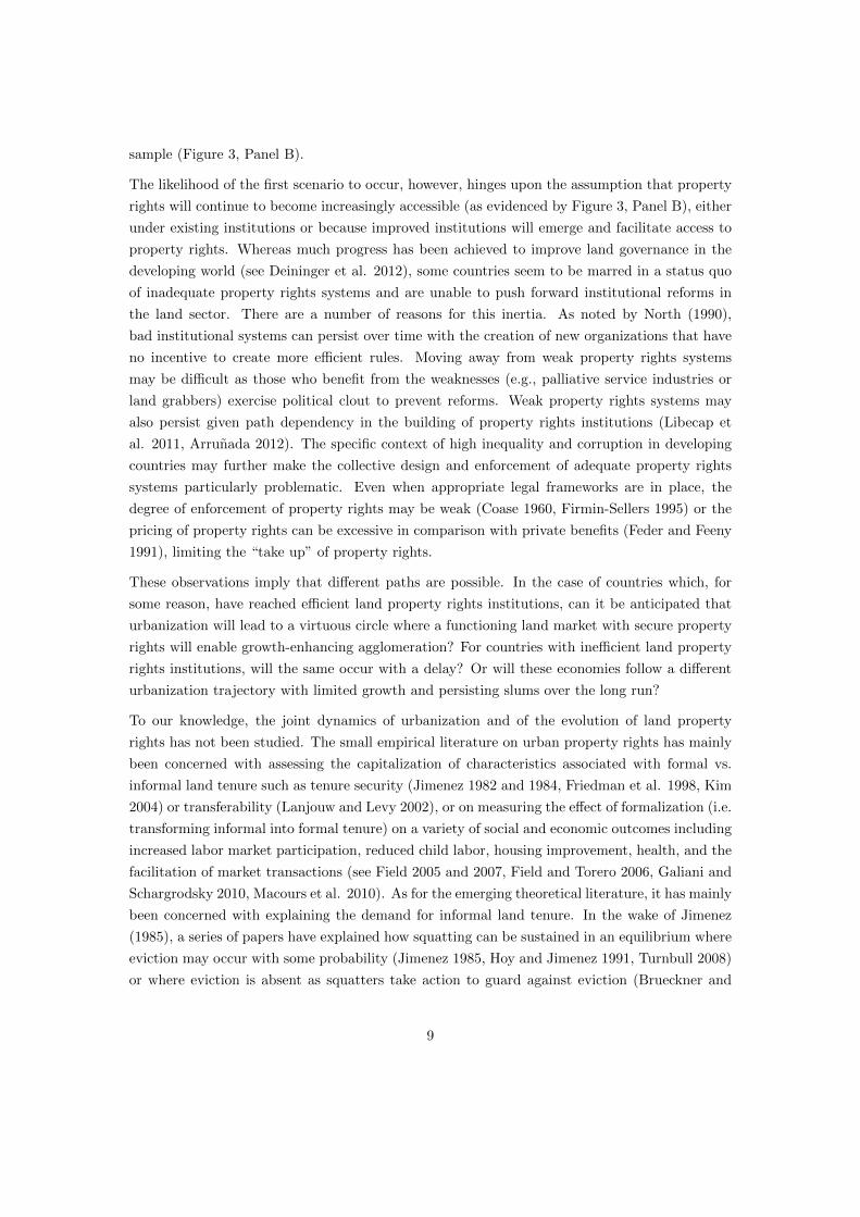
sample (Figure 3, Panel B).

The likelihood of the first scenario to occur, however, hinges upon the assumption that property

rights will continue to become increasingly accessible (as evidenced by Figure 3, Panel B), either

under existing institutions or because improved institutions will emerge and facilitate access to

property rights. Whereas much progress has been achieved to improve land governance in the

developing world (see Deininger et al. 2012), some countries seem to be marred in a status quo

of inadequate property rights systems and are unable to push forward institutional reforms in

the land sector. There are a number of reasons for this inertia. As noted by North (1990),

bad institutional systems can persist over time with the creation of new organizations that have

no incentive to create more efficient rules. Moving away from weak property rights systems

may be difficult as those who benefit from the weaknesses (e.g., palliative service industries or

land grabbers) exercise political clout to prevent reforms. Weak property rights systems may

also persist given path dependency in the building of property rights institutions (Libecap et

al. 2011, Arrunada 2012). The specific context of high inequality and corruption in developing

countries may further make the collective design and enforcement of adequate property rights

systems particularly problematic. Even when appropriate legal frameworks are in place, the

degree of enforcement of property rights may be weak (Coase 1960, Firmin-Sellers 1995) or the

pricing of property rights can be excessive in comparison with private benefits (Feder and Feeny

1991), limiting the “take up” of property rights.

These observations imply that different paths are possible. In the case of countries which, for

some reason, have reached efficient land property rights institutions, can it be anticipated that

urbanization will lead to a virtuous circle where a functioning land market with secure property

rights will enable growth-enhancing agglomeration? For countries with inefficient land property

rights institutions, will the same occur with a delay? Or will these economies follow a different

urbanization trajectory with limited growth and persisting slums over the long run?

To our knowledge, the joint dynamics of urbanization and of the evolution of land property

rights has not been studied. The small empirical literature on urban property rights has mainly

been concerned with assessing the capitalization of characteristics associated with formal vs.

informal land tenure such as tenure security (Jimenez 1982 and 1984, Friedman et al. 1998, Kim

2004) or transferability (Lanjouw and Levy 2002), or on measuring the effect of formalization (i.e.

transforming informal into formal tenure) on a variety of social and economic outcomes including

increased labor market participation, reduced child labor, housing improvement, health, and the

facilitation of market transactions (see Field 2005 and 2007, Field and Torero 2006, Galiani and

Schargrodsky 2010, Macours et al. 2010). As for the emerging theoretical literature, it has mainly

been concerned with explaining the demand for informal land tenure. In the wake of Jimenez

(1985), a series of papers have explained how squatting can be sustained in an equilibrium where

eviction may occur with some probability (Jimenez 1985, Hoy and Jimenez 1991, Turnbull 2008)

or where eviction is absent as squatters take action to guard against eviction (Brueckner and

9

Selod 2009, Brueckner 2013, Shah 2014).7 Departing from the restricted focus on squatters, Selod

and Tobin (2015) model the formalization choices of households in a context where land plots

may be appropriated by others due to multiple sales. In their model, higher endogenous land

prices in the core city provide greater incentives to formalize than at the periphery. Because all

these models are static—with the only exception of Turnbull (2008), who explores the strategic

choices of landowners regarding the timing of squatter eviction—none of them accounts for the

transformation of property rights over time under evolving land prices.

Our paper fills this important gap by proposing a theory that accounts for the joint dynamics

of urbanization and the evolution of property rights. We model urbanization through the mi-

gration of heterogeneous agents from a representative rural area to a representative city. The

prevalence of land tenure informality is determined by urban dwellers’ decisions whether and

when to purchase a property right. As land prices increase with agglomeration, formalization

becomes more desirable. However, formalizing may be too costly for less productive workers.

These workers who may not be able to afford both a land plot and a land title, will postpone the

decision to formalize, making themselves potential prey to land grabbers. The model can flexibly

account for the variety of situations regarding urbanization dynamics as its behavior critically

depends on key parameters regarding institutional quality (the cost and enforcement strength of

land property rights), the potential for agglomeration effects, and macroeconomic uncertainty.

Contrary to the modernization view of slums, and in line with the observation that “informality

may be here to stay”, it allows us to exhibit plausible contexts in which land tenure informality

remains in the long run. Deconstructing common-sense intuitions, the model also sheds lights on

situations where some level of informality is actually socially desirable. This is because, under

the parameters of the economy, informality provides access to the city to low income workers

who would not be able to contribute to the urban economy under compulsory formal property

rights. In this context, enforcement of strict eviction policies would be counter-productive. The

model also provides insights into leaving urbanization to the market, which can be suboptimal

under adverse structural parameters, in particular when the potential for agglomeration is low

and when land administration charge high fees.

The rest of the paper is organized as follows. Section 2 below presents the model which takes the

form of a discrete-time dynamic stochastic game under infinite time but a finite number of states

and actions. Section 3 then presents our concepts of social planner and decentralized solutions.

Section 4 explains our calibration before Section 5 presents the main results from simulations.

2 The model

We consider an economy with a set of N individuals. Individuals live forever and may either

reside in the rural area or in the city. In the city, individuals are exposed to a risk of conflict

7For a detailed survey, see Brueckner and Lall (2014).

10

over land that may result in their eviction from the plot they occupy (a “land grab”). Urban

dwellers can nevertheless pay to establish a property right on their plot instead of holding it

informally. Whereas informally holding a plot does not provide tenure security, formally held

plots are protected against land grabs and their owners cannot be evicted. Formally, let us

denote xit = (xU,it , xF,it ) the vector of state variables for a representative individual i at time t.

xU,it is the location variable for individual i. It takes value 1 if the household resides in the urban

area and 0 if the individual resides in the rural area at time t. xF,it is the property right variable.

xF,it takes value 1 if the household holds a property right at time t and 0 otherwise. We assume

that property rights can only be obtained in the urban area so that living in the rural area with

a property right is never a possibility in the model.8

When living in the city over the period (t, t + 1), the individual i earns a wage wU,it for his

work during the period but faces a congestion costs ct, which we assume to be the same for all

individuals. If residing in the rural area, the individual earns rural income wRt which we assume

is the same for all rural dwellers.9 There is no congestion cost in the rural area. Wages and the

urban congestion cost will be endogenous in the model. In addition, if settling in the city at

time t, an individual must purchase a land plot at a price Rt on the land market. Although the

price of land is endogenous in the city, because land is abundant in the rural area, we assume for

simplicity that the price of land in the rural area is equal to zero without any loss of generality.10

In our dynamic setting, the land price in the city is determined at the beginning of each period

by a macro-economic relation that accounts for city composition and economic conditions (see

below). The prevailing land price then drives location choices and grabbing decisions within the

period, which in turn affects the fundamentals of the land price for the next period. We assume

that there are absentee landlords who, in each period, sell land to urban in-migrants upon arrival

to the city and purchase it from voluntary out-migrants upon departure from the city, as well as

from land grabbers who resell grabbed land. In our modeling, absentee landlords are price takers

over a single period of time. They play the role of “market makers” allowing for a simplified

representation of the land market.11

8The prevalence of property rights in rural areas is very low in many countries. This is the case for instancewhen tenure in rural areas is overwhelmingly customary. Some countries may not have a land registration systemor a cadastre for rural areas. Relaxing this assumption would not change the main outcomes of the model whileadding unnecessary complexity.

9Productivity in the rural area is low and does not depend on individual intrinsic characteristics.10Rt could also be interpreted as the time-varying difference between the urban and rural land prices. Under

this alternative definition—which would assume an initial land endowment in the rural area for each individual—Rt would be much smaller than under the previous definition as it would only represent the fraction of incomeneeded to complement the proceed of the rural land sale to purchase an urban plot. The two definitions for Rtare mathematically equivalent in our setting under the assumption of a zero price for rural land.

11The existence of absentee landlords is also a standard assumption in static urban economics model wherethey sell land to households competing for land (see Fujita 1989).

11

2.1 Decisions

At the beginning of each period (t, t+ 1), an individual makes two choices: whether to migrate

and whether to purchase a property right.

Let us denote dit = (dU,it , dF,it ) the vector of choice variables made by individual i, where dU,it is

the migration decision and dF,it is the land tenure decision.

dU,it takes the value 1 when the individual decides to migrate to (or remain in) the urban area

between time t and t+ 1, and the value 0 if the individual decides to migrate to (or remain in)

the urban area between time t and t+ 1.

Because property rights provide protection against land grabs, formality is preferable over in-

formality. It is, however, costly to establish: an individual residing on an informal plot in the

city at time t needs to decide whether to pay a formalization fee ft to obtain a property right

between time t and t+ 1 or not to pay anything and continue to hold the plot informally.12 The

fee is proportional to the value of the land:

ft = µ.Rt (1)

with 0 < µ < 1. It is a one-time payment (e.g. registration in a cadastre) and does not need to

be paid again in subsequent periods as long as the individual uses the plot, i.e. as long as the

individual remains in the city. dF,it , the land tenure choice variable, takes the value 1 when the

individual decides to establish a property right between time t and t + 1 and takes the value 0

otherwise.

2.2 Shocks

Individuals move in and out of the urban area and in and out of residential formality throughout

their infinite lifetime. Movements between locations and between land tenure situations are

governed by migration and land tenure decisions (as individuals may seek property rights when

residing in the city) in the face of productivity shocks and land grab shocks.

Let us start with shocks and denote εit = (εPt , εG,it ) the vector of shocks faced by individual i in

period (t, t+ 1).

Firstly, εPt is a negative productivity shock (such as a weather shock) that affects the wage in

the rural area in period (t, t + 1). εPt takes the value 1 when the shock occurs and 0 otherwise.

This occurs with exogenous probability πP .

12In practice, fees can be paid for the formalization of an informally held plot, or following transactions offormal plots to ensure that they do not revert to informality (for instance by paying to update the registry withthe new owners’ name).

12

Secondly, εG,it is a “land grab opportunity” that affects informal urban dwellers to the potential

benefits of land grabbers. εG,it takes the value 1 if an opportunity to grab the plot of individual

i arises between time t and t + 1 and 0 otherwise. The shocks εG,it for i = 1, .., I are assumed

to be i.i.d. and occur with exogenous probability πG. πG reflects tenure insecurity on informal

plots. It may reflect the probability that an agent of the land administration or a judge will be

willing to facilitate an eviction. It also inversely reflects the degree of protection that informal

dwellers may have under current legislation and practices (e.g. if evictions are banned by local

authorities and if this ban is implemented, then πG = 0). Only plots faced with a land grab

opportunity (εG,it = 1) and which are not held formaly (xF,it = 0) will be grabbed or evicted. We

will present this in more detail below, after a brief presentation of the timing of decisions and

shocks..

2.3 Timing of decisions and shocks

In the model, state variables (xU,it and xF,it ) are defined at discrete points in time generically

denoted t. Decisions (dU,it and dF,it ) and shocks (εPt and εG,it ) occur within time periods generically

denoted [t, t+1).13 We specify here the exact timing of events within a period [t, t+1). We assume

the following sequence: at time t, individuals are located either in the city or the rural area and

may or may not have a property right. Shortly after time t, individuals simultaneously decide

where they want to locate (possibly relocate) and whether they want to purchase a property

right (if they have not done so earlier for the plot they occupy). Immediately after this decision

is made, they may then migrate (possibly involving the sale or purchase of land from absentee

landlords) and pay for the property right for those settling in the city and wishing to formalize.

In the first half period (t, t + 0.5), the city faces land grab opportunity shocks (idiosyncratic

probabilities of land grab opportunities are drawn). At time t + 0.5, land plots exposed to

grabbing are grabbed if unprotected (see below). . Land grab activities can affect urban wages

for the second half of the period (through a change in the city composition as individuals that lose

their plot are forced to move to the rural area shortly after time t+0.5).14 The rural productivity

shock occurs at t+ 0.5 and affects location decisions in the next period. It is important to note

here that, in order to be consistent with the nature of our shocks and our modeling of the land

market, we assume a period length of several years (exactly 10 years in our simulations).15

13We index these middle-of-the-period shocks, along with intermediary variables introduced later, with subscriptt.

14The relocations that occur shortly after time t+0.5 only reflect land grabs and do not result from the locationdecision which is made at time t and implies relocation shortly after time t.

15We assume that land can be fully purchased within one period, which requires a mid-term time horizon.Choosing relatively long periods does not qualitatively alter the results of the model. Calibrated parameters arechosen accordingly.

13

2.4 Migration

Individuals may choose to migrate between the rural area and the city in response to the difference

in the urban and rural incomes (net of housing and congestion costs) and given tenure insecurity

in the city and the possibility to formalize and the cost of formalization. In our model, in each

period, the rural-urban difference in income is affected by the rural productivity shock at time

t+0.5, implying:

wRs =

WRt,1 ≡ wR for s ∈ (t, t+ 0.5]

WRt,2 ≡ wR.(1− ηεPt ) for s ∈ (t+ 0.5, t+ 1]

(2)

where wR is agricultural productivity in the “good” state of the nature, and wR.(1 − ηεPt ) is

agricultural productivity in the “bad” state of the nature when the rural productivity shock εPt

(e.g. low rainfall) kicks in. η is the rural income elasticity to the shock with 0 < η < 1.

2.5 Land grabs / evictions

Formal and informal residents in the city may grab land from other informal residents after a

land grab opportunity arises (εG,it =1) for an urban plot that is informally held. Let us denote

It the set of informal dwellers in the city during the first half period (t, t+ 0.5) before the land

grab opportunity shocks happen. These are households who choose to live in the city at the

beginning of the period (dU,it = 1), who did not hold a formal property right at the beginning

of the period (xF,it = 0), and who did not become formal during the period (dF,it = 0). By

definition, It ={i|dU,it .(1− xF,it ).(1− dF,it ) = 1

}or It =

{i|dU,it .(1− xF,it+1) = 1

}. The land grab

opportunity shocks are drawn at a time in (t, t + 0.5), defining a subset IRt j It of informal

residents at risk of being grabbed, with IRt ={i|εG,it .dU,it .(1− xF,it+1) = 1

}. At time t + 0.5, if a

plot i∈ IRt , is grabbed, grabbers can immediately sell off the plot on the land market (to absentee

landlords) at the prevailing market land price Rt. The set of informal dwellers who get grabbed

IGt j IRt is defined by

IGt =

IRt , if IRt 6= Ht∅, if IRt = Ht

(3)

where Ht ={i|dU,it = 1

}is the set of city dwellers over (t, t+ 0.5].16

The aggregate profit from land grabbing in period t is

16IRt = Ht is the pathological case where all individuals should be grabbed but no one would be left in the cityto be a grabber, which cannot be possible. In this (unlikely case), we simply assume that no one gets grabbed inthe period.

14

PGt =∑i∈IGt

Rt =

N∑i=1

Rt.εG,it .dU,it .(1− xF,it+1) (4)

We assume that the land grabbing profit is redistributed to all remaining city-dwellers i∈ J t.17

Because richer (and more powerful) households are more likely to exert grabbing, we assume

that the share of the grabbing profit redistributed to each individual is proportional to that

individual’s wage wit.18 Each individual remaining in the city after t+ 0.5 (i ∈ Jt) thus obtains

an additional income from grabbing activities:

Git = PGtwit∑i∈Jt w

it

(5)

2.6 Agglomeration and congestion

Considering that an individual resides in the city during time sub-interval (t, t+ 0.5] if and only

if dU,it = 1, and during time sub-interval (t + 0.5, t + 1] if and only if xU,it+1 = 1, the population

size in the city for those two time intervals can be expressed by the formula

Ns =

∑Ni=1 d

U,it , for s ∈ (t, t+ 0.5]∑N

i=1 xU,it+1, for s ∈ (t+ 0.5, t+ 1]

(6)

There are benefits and costs associated with an increasing urban population, which we present

sequentially. Benefits are captured through agglomeration effects, where the productivity (and

thus the wage) of each individual in the city depends on the size and composition of the urban

labor force (see Duranton, 2013) as well as on land tenure. The latter assumption reflects the fact

that informal plot owners have a reduced labor supply as shown for example by Field (2007) in

the case of Lima, Peru. Assuming that each individual is characterized by an exogenous ability

ai > 0 and contributes ai units of labor to production when residing formally in the city and

(1 − κ).ai with 0 < κ < 1 when residing informally in the city, we can further define the total

efficient labor in the city as

Ls =

Lt,1 =∑Ni=1 ai.

(1− κ.(1− xF,it+1)

).dU,it for s ∈ (t, t+ 0.5]

Lt,2 =∑Ni=1 ai.

(1− κ.(1− xF,it+1)

).xU,it+1 for s ∈ (t+ 0.5, t+ 1]

(7)

If residing in the urban area, the wage of individual i can then be specified as

17The set of non-grabbed dwellers is Jt = Ht�IGt . It includes all urban households who were not grabbed in

period t. It is easy to see that Jt ={i|dU,it .

(1− εG,it .(1− xF,it+1)

)= 1}

or Jt ={i|xU,it+1 = 1

}.

18Alternatively, we could have considered that redistribution occurs with equal shares 1|Jt|

or that it reflects

an idiosyncratic ability or willingness to exert corruption.

15

wU,is =

WU,it,1 ≡ ai.σ. [1 + Lt,1]

1/γfor s ∈ (t, t+ 0.5]

WU,it,2 ≡ ai.σ. [1 + Lt,2]

1/γfor s ∈ (t+ 0.5, t+ 1]

(8)

where σ > 0, and γ > 0. 19

Let us now turn to congestion. For simplicity, we assume that congestion translates into a

monetary cost borne by city dwellers and is expressed in monetary units. It is measured by a

congestion function which depends on the size of the city.20 We have

cs = b. [Ns]δ

=

Ct,1 ≡ b.[∑N

i=1 dU,it

]δfor s ∈ (t, t+ 0.5]

Ct,2 ≡ b.[∑N

i=1 xU,it+1

]δfor s ∈ (t+ 0.5, t+ 1]

(9)

where Ns is defined by (6), for s ∈ (t, t + 1]. Here, wis, cs, Wit,1, W i

t,2, Ct,1, Ct,2 are measured

per period. Because of the existence of possible shocks, both W it,2 and Ct,2 are random.

Equation (9) captures the negative externalities associated with agglomeration.21

2.7 Land prices

As for land costs, they are only incurred upon arrival in the city (when the individuals need to

purchase a land plot). We assume that each individual consumes one unit of land and that there

is a unique price for land in the city at any given point in time.22 We assume that the ratio of

the land price to the average income is constant. This long-term relation has been established

at the city level both theoretically and empirically in the literature (see Ried and Uhlig, 2009,

Malpezzi, 1999, and Leung, 2014). Since transactions only occur during the first half of the

period (households purchase or sell land at the beginning of the period, and grabbers sell off

grabbed land at time t + 0.5), the price is a function of the population and wage that prevail

during (t, t+ 0.5], so we have

Rt = λ.

∑Ni=1W

U,it,1 .d

U,it∑N

i=1 dU,it

(10)

19The formula can be derived by assuming a production function

Y =σ.[1 + L]1/γ+1

1/γ + 1

with wit = aidYdL

.20Congestion here reflects the various externalities associated with city size, including travel distance and time

(Izraeli and McCarthy, 1985), pollution (Lamsal et al., 2013) or criminality (Glaeser and Sacerdote, 1999).21The formula can be derived as the average transport cost in a mono-centric city with convex transport costs

(see Fujita, 1989).22This can be viewed as the average price of land in the city. We could adopt a more sophisticated representation

of land with prices that vary depending on within-city location as in Selod and Tobin (2015) but this would makethe model more complex without affecting the main results.

16

where 0 < λ < 1 .23

2.8 Land transactions

Land is transferred whenever there are population movements between the city and the rural

area or when land is grabbed (and immediately sold off).

Migrants to the city only purchase land upon arrival. We can thus define a variable that measures

land purchases as P it = Rt if individual i arrives in the city shortly after time t and P it =0

otherwise. This is modeled using the formula

P it=Rt.dU,it .(1− xU,it ) (11)

Conversely, individuals who voluntarily decide to leave the city shortly after time t sell their land

back upon departure at a price Rt. We can define a variable that measures land sales as Sit =Rt

if individual i voluntarily leaves the city during period (t, t+ 1] and Sit =0 otherwise.24 This is

obtained for25

Sit = Rt.(1− dU,it ).xU,it (12)

2.9 Location and land tenure transitions

We now turn to the general definition of transitions, which are defined by the correspondence

Γ : xit 7−→ xit+1 as a function of xit ,dit and εit where xit ∈ {0, 1}2, dit ∈ {0, 1}2 and εit ∈ {0, 1}2.

This correspondence completely defines what happens between time t and time t + 1 to the

location and tenure (state variables) of an individual in all possible states and facing all possible

combinations of shocks.

We can now infer the laws of motion that fully characterize the transitions between t and t+ 1

as functions of states at time t and decisions and shocks between time t and time t+ 1. We have

xU,it+1 = dU,it .max{xF,it , dF,it , 1− εG,it

}(13)

23

Although the land price fluctuates within each period because of involuntary population movements betweenthe first and the second half of each period, transactions only occur at the beginning of the first halfof the period following voluntary location decisions. We also assume that sales of grabbed land occurat the current land market price, which can be justified by stickiness.

24Individuals who are victim of a land grab must leave the city and cannot recoup their land investment.25Note that in each period the total net payment received by absentee landlords is Πt =

∑Ni=1

(P it − Sit

)−∑

i∈IGtRt, which can be positive or negative. In the long run, when the population of the city and the share of

informal dwellers stabilize, this is expected to be zero as there will be as many sales as purchases.

17

xF,it+1 = dU,it .max{xF,it , dF,it

}(14)

Transition formula (13) states that in order to reside in the city at time t+ 1, individual i must

have decided to remain in or to move to the city between time t and t+1 and either already held

a property right for his urban plot at time t, decided to formalize between time t and time t+ 1,

or did not face a land grab shock between time t and t + 1. Transition formula (14) recognizes

that to have a property right at time t+ 1, the individual must have decided to remain in or to

move to the city between time t and t + 1 and either already had a property right at time t or

acquired one between time t and t+ 1.

3 Stochastic game and social planner solution

We will now determine how the system evolves under two different optimization problems and

associated solution concepts (stochastic game and social planner optimum). This involves de-

termining how states at the beginning of one period are followed by policy functions during

the period (decisions in our framework) that determine states at the beginning of the following

period. To do this, let us define the strategy for individual i as the function from the vector

of states xt ={

(xU,it , xF,it )i=1,...,N

}into individual decisions dit = (dU,it , dF,it ), which we simply

denote Dit(xt).

26

To understand how strategies are determined, we now need to understand how individuals are

affected by decisions. To do that, observe that at time t, when individual i decides to live in

the rural area during the period (t, t+ 1] (i.e. dU,it = 0), he will receive(WRt,1 +WR

t,2

)/2 + Sit in

the period. When individual i decides to live in the urban area during the period, he will pay

dF,it .ft + P it at the beginning of the period, receive wage WU,it,1 /2 and incur the congestion cost

Ct,1/2 during the first half period. During the second half period, if the individual is forced to

leave the city because he faced a land grab opportunity at t + 0.5 (i.e. εG,it = 1) and did not

have a property right (i.e., xF,it+1 = 0), then he will receive WRt,2/2; otherwise, he will receive a

wage WU,it,2 /2, incur a congestion cost Ct,2/2, and receive his fraction of the land grab proceeds

Git . The net income of the individual who decides to reside in the city in (t, t+ 1) is thus

yt =

12

(WU,it,1 − Ct,1 +WR

t,2

)− P it if εG,it =1, xF,it+1 = 0,

12

(WU,it,1 − Ct,1 +WU,i

t,2 − Ct,2)

+ Git − dF,it .ft − P it otherwise.

Thus, we have the utility of individual i over the period (t, t+ 1]

26Note that because decisions are made before shocks occur in each period, they are only functions of thecurrent states but not of the realization of the shocks.

18

uit = ui(xt,dt) =

((WR

t,1+WRt,2)/2+S

it)

1−α

1−α if dU,it = 0,

y1−αt

1−α otherwise.(15)

The relevant part of the expression when the individual decides to reside in the rural area does

not include the term dF,it .ft because, by definition, a household will not simultaneously decide

to formalize and migrate to the rural area. The specification reflects risk-aversion through the

parameter α.

With the above framework, we can now solve the two different optimization problems that

respectively correspond to the social planner solution or the stochastic game solution that results

from individual choices.

3.1 Social planner solution

At the beginning of each period t, the planner assigns to individuals a sequence of location and

formalization decisions so as to maximize the expected value of the sum of discounted stream of

aggregated utilities and profits, considering the exogenous shock probabilities (and likelihood of

transitions between states). The social planner’s objective function at time t is

max{dt,dt+1,...}

E

[U(xt,dt) +

∞∑τ=t+1

βτ−t.U(xτ ,dτ )

](16)

where U(xt,dt) =∑Ni=1 u

it(xt,dt) aggregates individual preferences and E is the expectation

operator27 and β ∈ (0, 1) is the discount factor and the expectation is taken over the random

productivity and land grab opportunity shocks. Note that the shocks enter in (16) through xτ

which, as we have seen, is a function of xτ−1, dτ−1 and ετ−1. The transition laws of xt are

given by (13) and (14) for each individual. For simplicity, we denote the transition laws as

xt = g(xt−1,dt−1, εt−1).

Because it is an infinite-horizon problem, the decision depends only on the current state and we

can write the corresponding Bellman equation (Bellman, 1957) as

V s(x) = maxdE {U(x,d) + β.V s(x+)} (17)

where x is the current-period state, and x+ is next-period state dependent on x, decision d, and

the shocks ε, i.e., x+ = g(x,d, ε). The optimal policy function is Di(x) for individual i.

Definition of social planner solution: We define the social planner solution as the value function

V s(x) and the set of individual policy functions D(x) ={Di(x) : i = 1, ..., N

}that solve the

Bellman equation (17) given the Social Welfare Function U .

27We consider a utilitarian social welfare function but any other social welfare function can be used.

19

The right-hand side of the Bellman equation (17) can be expressed as Γ (V s)(x) where Γ is the

Bellman operator. We see that the value function V s(x) is a fixed point of the Bellman operator,

so we can use an iterative method to find V s(x). We apply the value function iteration, that is, we

first choose an initial guess of V s(x), denoted as V s0 (x), and then compute V st (x) = Γ (V st−1)(x)

for t ≥ 1 until the iteration converges. A detailed discussion of value function iteration is available

in Judd (1998).

3.2 Stochastic game

Here we are trying to solve the stochastic game problem where every individual wants to maximize

the present value of his own expected stream of utilities. Mathematically, instead of (16), we

now have the multi-objective optimization problem:

max{dit,dit+1,d

it+2,...}

E

[ui(xt,dt) +

∞∑τ=t+1

βτ−tui(xτ ,dt)

]for i = 1, ..., N (18)

Note that xt and dt are still states and decision vectors for all individuals in the economy.

Since every individual has his own value function V i(x) and policy function Di(x) which depend

on the states of all individuals, we also need to replace (17) with the following set of Bellman

equations (one per individual):

V i(x) = maxdi

E{ui(x,d) + β.V i(x+)

}for i = 1, ..., N (19)

where x+ = g(x,d, ε).

In this context, our concept of equilibrium is the stationary Markov-perfect equilibrium as in

Maskin and Tirole (1987, 1989a, and 1989b).28 It is a natural equilibrium concept to adopt in a

dynamic setting such as ours where individuals optimize their own discounted utility taking into

account other individuals’ decisions.

Definition of equilibrium: We define a stationary Markov-perfect equilibrium as the set of value

functions Vall(x) ={V i(x) : i = 1, ..., N

}and the set of individual policy functions D(x) ={

Di(x) : i = 1, ..., N}

such that for any individual i = 1, ..., N and for any vector of states x

and other players’ actions d−i =(d1, ...,di−1,di, ...,dN

)with dj = Dj(x) for j 6= i, the value

function V i(x) solves the Bellman equation in (19), and the individual strategy Di(x) solves the

right-hand side of the equation (19).

We denote the right-hand side of the system of Bellman equations F(Vall)(x), where F is

the Bellman operator vector. Vall(x) is the fixed point of F . Thus, as for the the social

28The same equilibrium concept has been widely applied in the literature on industry dynamics, see e.g., Ericsonand Pakes (1995), Maskin and Tirole (2001), and Doraszelski and Satterthwaite (2010).

20

planner problem, we can also solve for Vall(x) by applying an iterative method. However, it

is time consuming to compute F for problems with large N , because of three levels of “curse-

of-dimensionality”, whereby computational cost increases exponentially in the number of state

variables, the number of decision variables, and the number of shock variables for computing

expectation. To address this issue Pakes and Mcguire (1994) introduced a computational method

for computing Markov-perfect Nash equilibria for stochastic games with continuous choices. In

a related work, Doraszelski and Judd (2012) analyze continuous-time stochastic games to avoid

the curse of dimensionality in computing expectations. In this paper, we use a variant of the

method of Pakes and Mcguire (1994) to find a stationary Markov-perfect equilibrium for our

discrete-time, infinite-horizon stochastic game with discrete states and discrete choices. That

is, we choose the optimal policy functions of the social planner problem as our initial guess

of D(x) for the stochastic game, denoted as D0(x) ={Di

0(x) : i = 1, ..., N}

. We then let

the initial guess of Vall(x) be Vall0 (x) = E

{ui(x,D0(x))

}/(1 − β). Denoting (D−it (x),di) =

(D1t (x), ..., Di−1

t (x),di, Di+1t (x), ..., DN

t (x)), we compute

V it (x) = maxdi

E{ui(x,D−it−1(x),di) + β.V it−1(x+)

}, (20)

for each i = 1, ..., N , and let Dit(x) be the optimizer for individual i at the t-th iteration for t ≥ 1.

At iteration t, we know the value function and policy functions at the previous iteration t − 1

for every individual. Each individual determines his own optimal decision under the assumption

that the other individuals make their decisions at t that replicate their policy functions at t− 1.

Note that although the F operator has to be solved jointly for all individuals, equation (20) can

be solved separately for each individual i. This makes equation (20) much easier and faster to

solve. We iterate over t until both Vallt and Dt(x) converges. The converged value and policy

functions are the solution to the stochastic game.

From Maskin and Tirole (2001), we know that there exists a Markov-perfect equilibrium for

our stochastic games with finite action spaces. However, our stochastic games may still have

multiple equilibria, although Maskin and Tirole (2001) point out that the Markov-perfect equi-

librium concept, a refinement of the Nash equilibrium, can be applied to eliminate or reduce

the multiplicity of equilibria in dynamic games. Recently, Borkovsky et al. (2010) applied the

homotopy approach to detect equilibrium multiplicity for games with continuous strategies, and

Judd et al. (2012) developed all-solution homotopy methods to find all equilibria of static and

dynamic games with continuous strategies. Yeltekin et al. (2015) provide a numerical method

for computing all subgame-perfect equilibria of dynamic games with both discrete and continu-

ous strategies, but their examples consist of only two or three-player dynamic games even with

massive parallelization. As our examples are stochastic games and have a large number of players

(in our example N = 5 players and 2N = 10 dimensions of states), it is still challenging to find

all equilibria for such a large-dimensional problem, so we leave this for future research.

21

4 Model calibration

We choose values for the model parameters based on econometric estimates in the economic

literature on urbanization and development. When econometric estimates are not available,

we calibrate the remaining model parameters to match observed patterns of urbanization in

developing countries. For most significant model parameters, we conduct a sensitivity analysis

over the range of their plausible values. Table 1 lists the model’s parameters and shows the

chosen values.

We set the number of economic agents to 5 in order to balance the model’s computational

feasibility with tractability. We interpret the number of agents as population quantiles. We

consider a uniform distribution of abilities over (0, 1] with ai = i/N for i = 1, ...N . Agent N is

thus the individual of highest ability aN = 1. We normalize the before-productivity-shock rural

wage wR to 1. We set the informal residency penalty on productivity κ equal to .2, consistently

with Field (2007). We choose a value of 3 for σ. In developed economies for which state-of-

the-art studies control for sorting according to ability, an increase in city size of 10 percent

causes productivity to increase by between .3 and .8 percent (Duranton, 2009). We thus choose

a benchmark value of γ of 11, which yields productivity increases of .4 to .7 percent depending

on city size.29 We choose a value of .2 for the rural wage elasticity to adverse shocks, η, based on

Jayachandran (2006) who estimated an rural wage elasticity of 17 percent to a weather shock.

Wet set the probability of adverse income shock in rural area, πP , to .3 based on Damberg

and AghaKouchak (2013), who report 12 episodes between 1979 and 2013 where more than 20

percent of the land in the Southern Hemisphere was under moderate to severe drought. This

corresponds to a drought every three years or a yearly probability of a drought of approximately

1/3.30

As regards the congestion cost parameters, we choose a value of 1 for b and .3 for δ. These

numbers are based on the average of Kahn (2010) estimates, who reports city-size elasticities of

.14, .25 and .49 for commute times, carbon monoxide pollution and for violent crime respectively.

Our choice of λ is based on Malpezzi (1999), who reports a median housing price-to-income ratio

in 133 US MSAs of 4.5. Assuming that land represent two-thirds of total housing costs and

considering that our period is 10 years, this leaves us with a value of .3.

For the formalization cost parameter, µ, we choose a value of .3. There is a wide variety of

situations in terms of formalization contexts, with costs ranging from a few percentages of land

value to up to 100 percent or more of the value of the land (see Durand-Lasserve et al., 2015).

For πG we assume a value of .1 which is consistent with the high prevalence of conflicts in the

cities of developing countries.

29In our model, wage elasticity with respect to urban labor force size is Lγ.(1+L)

. Since L is comprised between

1 and 5, a value of γ comprised between 10.4 and 16.6 ensures that wage elasticities are comprised between 0.03and 0.08 in any state of the economy.

30.3 is a conservative estimate as other shocks affecting incomes such as conflicts, natural disasters or healthcrises can also occur (see Zceleczky and Yosef, 2014).

22

Table 1: Parameter Values of Calibrated Model

Parameter Description ValueI Number of economic agents 5ai Agents’ ability {0.2,0.4,0.6,0.8,1}κ Informal residency productivity penalty 0.2σ Agglomeration scaling factor 3γ Income effect of agglomeration 5, 11, 100η Rural wage elasticity of adverse shocks 0.2b Congestion scaling factor 1δ Congestion elasticity of agglomeration 0.3λ Land price to rent ratio 0.3µ Cost of land tenure formalization 0.3, 0.9πP Probability of adverse shock in rural area 0.3πG Probability of land grab attempt / eviction enforcement 0.05, 0.1, 0.5α Risk aversion parameter 2β Discount rate (10 year period) 0.86

We set the value of the risk aversion parameter, α, to 2, which is consistent with reported

estimates in the meta-analysis conducted by Havranek et al. (2015). We use an annual discount

rate of .985, which is consistent with the number adopted by long run dynamic computational

forward-looking economic models, e.g., Nordhaus’ DICE model (Nordhaus, 2008). Given that a

period spans over 10 years in our model, this translates to (.985)10 = .86.

Given a significant range of heterogeneity for some model parameters, we conduct a sensitivity

analysis to demonstrate the model’s robustness to chosen parameter values. Specifically, we

analyze our results’ sensitivity to variations in following model parameters: (a) income effect of

agglomeration, γ, of 5 (high agglomeration potential) and 100 (low agglomeration potential); (b)

cost of land tenure formalization, µ, of .9 (high formalization cost); and (c) probability of land

“grab”, πG of .05 (low chance of eviction) and .5 (high chance of eviction).

5 Simulation Results

We solve equations (17) and (19) as explained in section 3 for a set of parameter values described

in section 4 to obtain the value functions that can be used to infer stationary states and corre-

sponding optimal decision rules. We then simulate dynamic urbanization paths corresponding

to the social optimum and the Markov perfect equilibrium based on the realization of randomly

drawn shocks εPt and εG,it .

Figure 4 illustrates one of such simulated paths that corresponds to solving for a Markov-perfect

equilibrium under a low formalization cost, low agglomeration potential and low risk of eviction.

For all simulations we start with an empty set of the city with no residents.31 We see that

31We have also run simulations for an alternative assumption of one, the most productive, informal urban

23

Figure 4: Example of Urbanization Path, Markov-perfect Equilibrium

Note. Simulated path assumes the following parameter values: γ = 100, µ = 0.3, πG = 0.05.

in the second period the most productive agent moves into the city, and stays informal. Next

period, this agent faces an increase in wage income and purchases a title for his plot. In period

4, another, less productive, agent moves into the city, and chooses to stay informal. The wage

incomes of both agents 4 and 5 increase thanks to the agglomeration effect and agent 4 chooses

to formalize. The stationary state is obtained in period 5 as agents 1, 2, and 3 do not find it

optimal to move into the city as the agglomeration potential is low. In this stationary state

the urbanization rate is 40 percent and the rate of informality is 0 percent (all urban residents

eventually choose to formalize their land plots). We can also see that welfare (defined as the

sum of agent’s discounted utilities∑V i in the stationary state and normalized to 100 in period

1 for illustration purposes) increases as agents move in the city and become formal. This result

is consistent with earlier theoretical and empirical evidence of the welfare improving aspects of

urbanization (Bertinelli and Black 2004) and secure property rights (Feder and Feeny 1991).

While Figure 4 is illustrative of the urbanization dynamics in our model, it is not generalizable

as each simulation path results in a different stationary state given initial states and the history

of productivity and land grab shocks. To obtain generalizable results, we simulate dynamic

urbanization and formalization paths 100,000 times for each initial state and parameter values,

resident in the initial state. The results were very similar.

24

and calculate the expected urbanization and land formality rates.

Figures 5 and 6 show expected urbanization and land formality rates that correspond to the

simulated Markov-perfect stationary equilibria (panel a) and social optima (panel b).32 Figure

5 illustrates the variations in urbanization and land formality outcomes given different sizes of

agglomeration potential and probabilities of land eviction when the land formalization cost is

low (µ = 0.3). Figure 6 shows the same simulation results when the land formalization cost is

high (µ = 0.9).

Beginning with Figure 5 (panel a), we see that when agglomeration potential is high and eviction

probabilities are low to moderate, the Markov-perfect stationary equilibria is consistent with an

expected urbanization rate of 60 percent. When the agglomeration potential is low or moderate

and eviction probabilities are high, the expected urbanization rate declines to 40 percent. Figure

6 (panel a), shows a similar pattern. These results lead to the following proposition:

Proposition 1a: The urbanization rate in the Markov-perfect stationary equilibrium increases

when (a) eviction enforcement is weak, and (b) agglomeration potential is high.

The underlying intuition behind Proposition 1a is as follows. The urbanization dynamics in our

model are driven by the realized benefits of moving to the city. Agents with lower abilities can

only find it individually optimal to move to the city when agglomeration potential is high enough

to compensate for the urban rent and congestion costs. Even in these situations the decision

to move to the city is not warranted. As their income is not sufficient to pay for formalization

costs, agents choose to stay informal for some time before they can afford paying for land titles.

When the probability of land eviction is high, low productive and risk-averse agents will find it

suboptimal to move to the city.

Now, let us turn to Figure 5 (panel b), which represents simulated results for the social optimum,

and let us compare these results to those from panel (a). We see that irrespective of variations

in model parameters, the expected urbanization rate is 60 percent. The expected urbanization

rates are the same for the social optimum and the Markov-perfect stationary equilibrium when

agglomeration potential is high and eviction probabilities are low to moderate. The expected

urbanization rates are, however, higher for the social optimum that for the Markov-perfect sta-

tionary equilibrium for low or moderate agglomeration potential and high eviction probabilities.

A similar pattern is observed when we compare panels (a) and (b) of Figure 6, although the

expected urbanization rate of 60 percent is not always sustained when land tenure formalization

costs are higher. These results lead to the following proposition:

Proposition 1b: The urbanization rate under the Markov-perfect stationary equilibrium is lower

than in the social optimum when (a) agglomeration potential is low, and (b) eviction enforcement

is strong.

32The numerical values of expected urbanization and land formalization rates that correspond to the modelsimulations are shown in appendix Table A.1.

25

Figure 5: Expected Urbanization and Informality Rates, µ = 0.3

(a) Markov Perfect Equilibrium

(b) Social Optimum

Note. Shaded areas correspond to the share of informal residents.

26

Figure 6: Expected Urbanization and Informality Rates, µ = 0.9

(a) Markov Perfect Equilibrium

(b) Social Optimum

Note. Shaded areas correspond to the share of informal residents.

27

To understand the logic behind Proposition 1b, it is important to recall the important distinction

between the allocation of urban residents under the social optimum and the Markov-perfect

equilibrium. In the Markov-perfect equilibrium, all agents move sequentially and make their

land formalization decisions simultaneously. In the social optimum all decisions are made by

the joint welfare-maximizing social planner, who has discretion over the timing of individuals

moving into the city. The social planner may then choose to move less productive agents into

the city first and allow them to obtain land titles before they can be evicted by more productive

agents entering the city. Proposition 1b makes an important claim that the path of urbanization

itself matters for final urbanization outcomes - an issue completely overlooked in static models

of urbanization.

Combining propositions 1a and 1b yields the following corollary:

Corollary 1: In cities that have low agglomeration potential and strong eviction enforcement, the

urbanization rate is low and lower than the social optimum.

This finding resonates well with the observed over-enforcement of evictions in the developing

countries. The model suggests that, in some contexts, local governments may have done more

harm than good by checking migration to cities through eviction of informal settlements (see Lall

et al., 2006, on the causes of over-restrictive internal migration policies and Durand-Lasserve and

Selod, 2009, on eviction policies). Over-enforcement of evictions may have caused some cities to

be undersized (i.e., overlooking the potential benefits of further agglomeration) in a way that is

similar to the enforcement of migration restrictions (see Au and Henderson, 2006, on the case of

Chinese cities).

The next important issue to investigate is that of land tenure formalization. We see from Figure

5 (panel a) that when land tenure formalization costs are low, all agents that choose to move

to the city also choose to formalize. This does not always happen when formalization costs are

high. Figure 6 shows that informal residency can be sustained in the Markov-perfect stationary

equilibrium when the eviction probability is low. If the city exhibits medium to high agglom-

eration potential, the observed informality rate is two-thirds. When the city’s agglomeration

potential is low, all residents are informal. These observations constitute the basis for the next

proposition:

Proposition 2a: Informality can be sustained in the long run in the Markov-perfect stationary

equilibrium. Informality is all the more likely to prevail as formalization costs are higher, evic-

tion enforcement is weak, and agglomeration potential is low. For low land formalization costs,

informality is resorbed.

The underlying explanation for Proposition 2a is fairly straightforward. Agents’ decisions to

formalize are determined by the difference between the expected marginal benefits of avoided

eviction and potential gains from evicting other informal residents, and the realized marginal

cost of formalizing land tenure. As the probability of land eviction declines, the latter effect

28

tends to dominate and no one formalizes. When the city’s agglomeration potential is low, the

city is smaller (Proposition 1a), and the expected gain from evicting other informal residents

diminishes. This, in turn, leads to an even higher share of informal residents in the city.

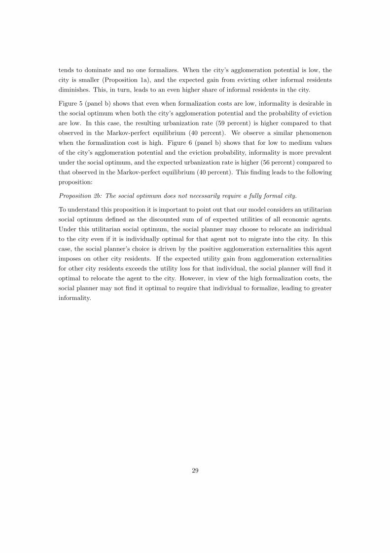
Figure 5 (panel b) shows that even when formalization costs are low, informality is desirable in

the social optimum when both the city’s agglomeration potential and the probability of eviction

are low. In this case, the resulting urbanization rate (59 percent) is higher compared to that

observed in the Markov-perfect equilibrium (40 percent). We observe a similar phenomenon

when the formalization cost is high. Figure 6 (panel b) shows that for low to medium values

of the city’s agglomeration potential and the eviction probability, informality is more prevalent

under the social optimum, and the expected urbanization rate is higher (56 percent) compared to

that observed in the Markov-perfect equilibrium (40 percent). This finding leads to the following

proposition:

Proposition 2b: The social optimum does not necessarily require a fully formal city.

To understand this proposition it is important to point out that our model considers an utilitarian

social optimum defined as the discounted sum of of expected utilities of all economic agents.

Under this utilitarian social optimum, the social planner may choose to relocate an individual

to the city even if it is individually optimal for that agent not to migrate into the city. In this

case, the social planner’s choice is driven by the positive agglomeration externalities this agent

imposes on other city residents. If the expected utility gain from agglomeration externalities

for other city residents exceeds the utility loss for that individual, the social planner will find it

optimal to relocate the agent to the city. However, in view of the high formalization costs, the

social planner may not find it optimal to require that individual to formalize, leading to greater

informality.

29

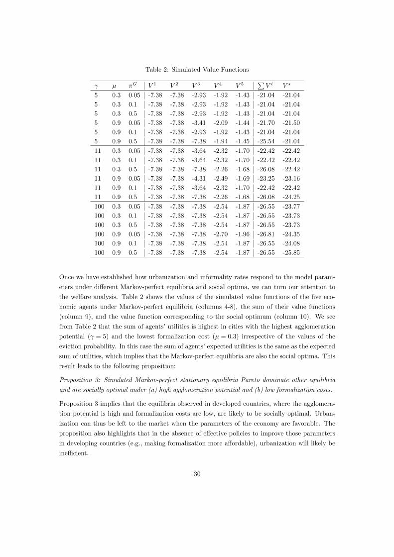
Table 2: Simulated Value Functions

γ µ πG V 1 V 2 V 3 V 4 V 5∑V i V s

5 0.3 0.05 -7.38 -7.38 -2.93 -1.92 -1.43 -21.04 -21.04

5 0.3 0.1 -7.38 -7.38 -2.93 -1.92 -1.43 -21.04 -21.04

5 0.3 0.5 -7.38 -7.38 -2.93 -1.92 -1.43 -21.04 -21.04

5 0.9 0.05 -7.38 -7.38 -3.41 -2.09 -1.44 -21.70 -21.50

5 0.9 0.1 -7.38 -7.38 -2.93 -1.92 -1.43 -21.04 -21.04

5 0.9 0.5 -7.38 -7.38 -7.38 -1.94 -1.45 -25.54 -21.04

11 0.3 0.05 -7.38 -7.38 -3.64 -2.32 -1.70 -22.42 -22.42

11 0.3 0.1 -7.38 -7.38 -3.64 -2.32 -1.70 -22.42 -22.42

11 0.3 0.5 -7.38 -7.38 -7.38 -2.26 -1.68 -26.08 -22.42

11 0.9 0.05 -7.38 -7.38 -4.31 -2.49 -1.69 -23.25 -23.16

11 0.9 0.1 -7.38 -7.38 -3.64 -2.32 -1.70 -22.42 -22.42

11 0.9 0.5 -7.38 -7.38 -7.38 -2.26 -1.68 -26.08 -24.25

100 0.3 0.05 -7.38 -7.38 -7.38 -2.54 -1.87 -26.55 -23.77

100 0.3 0.1 -7.38 -7.38 -7.38 -2.54 -1.87 -26.55 -23.73

100 0.3 0.5 -7.38 -7.38 -7.38 -2.54 -1.87 -26.55 -23.73

100 0.9 0.05 -7.38 -7.38 -7.38 -2.70 -1.96 -26.81 -24.35

100 0.9 0.1 -7.38 -7.38 -7.38 -2.54 -1.87 -26.55 -24.08

100 0.9 0.5 -7.38 -7.38 -7.38 -2.54 -1.87 -26.55 -25.85

Once we have established how urbanization and informality rates respond to the model param-

eters under different Markov-perfect equilibria and social optima, we can turn our attention to

the welfare analysis. Table 2 shows the values of the simulated value functions of the five eco-

nomic agents under Markov-perfect equilibria (columns 4-8), the sum of their value functions

(column 9), and the value function corresponding to the social optimum (column 10). We see

from Table 2 that the sum of agents’ utilities is highest in cities with the highest agglomeration

potential (γ = 5) and the lowest formalization cost (µ = 0.3) irrespective of the values of the

eviction probability. In this case the sum of agents’ expected utilities is the same as the expected

sum of utilities, which implies that the Markov-perfect equilibria are also the social optima. This

result leads to the following proposition:

Proposition 3: Simulated Markov-perfect stationary equilibria Pareto dominate other equilibria

and are socially optimal under (a) high agglomeration potential and (b) low formalization costs.

Proposition 3 implies that the equilibria observed in developed countries, where the agglomera-

tion potential is high and formalization costs are low, are likely to be socially optimal. Urban-

ization can thus be left to the market when the parameters of the economy are favorable. The

proposition also highlights that in the absence of effective policies to improve those parameters

in developing countries (e.g., making formalization more affordable), urbanization will likely be

inefficient.

30

Careful examination of Table 2 shows that other equilibria may not be ranked unanimously as

economic agents rank them differently. The expected agents’ utilities are non-monotonous func-

tions of (a) agglomeration potential, (b) eviction enforcement and (c) formalization costs. More

productive agents that choose to reside in the city may face a trade-off between maximizing their

wages (which depend on the city’s agglomeration potential and agent’s abilities) and increasing

their gains from potential land grabs of informal residents’ land plots as these two effects may

or may not go in the same direction.

To further elaborate on this point, consider a city with medium agglomeration potential (γ = 11).

We can see from Table 2 that, regardless of formalization costs, the social optimum is reached

for low to medium probabilities of eviction. Strict eviction enforcement deters in-migration of

less productive agents who cannot afford to pay for land tenure formalization before they can

establish themselves in the city. However, by looking at individual payoffs under different land

eviction regimes, we see that more productive agents (4 and 5) achieve higher levels of expected

utility when the eviction probability is high. For these agents, the marginal costs exceed the

marginal gains of having an additional agent migrate to the city. As these agents are likely to be

economic and political elites that establish themselves earlier in the city, their preferred eviction

regime may not necessarily reflect the socially optimal outcome. These observations combined

yield the following proposition:

Proposition 4: Strict eviction policies can be welfare reducing. It can be in the interest of the

society but not necessarily in the interest of city elites to accept some level of informality.

In line with Corollary 1, our model provides a theoretical insight into the political economy of

over-eviction policies. Although evictions remain widespread in many developing countries, it

is interesting to note that some countries have moved away from strictly enforced evictions and

modified their legal frameworks to provide protection against eviction (Durand-Lasserve 2007).

Proposition 4 suggests that more democratic contexts are favorable to such changes.

6 Conclusion

We analyze the interplay between urbanization and evolution of land property rights, two features

of economic development that interact in a very important way. Understanding this interaction is

crucial for developing countries as dysfunctional urban land property rights systems continue to

prevail in many parts of the developing world, and their implications for the path of urbanization

in the long run are not well understood. The model we develop provides a novel analytical

framework to study this issue. It is a dynamic stochastic model of a representative city that jointly

determines urbanization and evolution of land property rights. Each period, heterogeneous

households decide whether to live in the city or in a rural area, and whether to pay for land

property rights that will protect them from future eviction attempts. Holders of informal plots

are randomly exposed to land seizure by other city dwellers, and seized plots can be resold

31

on the land market. Population movements in and out of the city are thus affected both by

land grabbing and productivity shocks. Agglomeration and congestion effects are endogenous to

migration, affecting wages and land prices.

Our main result is that land property rights institutions, which are very difficult to reform,

have a significant effect on the dynamics of urbanization in the long run. Contrary to the

developed world experience, leaving urbanization to the market may be suboptimal because of

the constraints imposed by dysfunctional property rights systems in developing countries. We

also demonstrate that, under certain conditions, informality can be socially optimal, as it makes

it possible for low-income residents to contribute to the urban economy. In these situations,

strict urban eviction policies can be welfare reducing.

It is important to note that our major insights are conditional on structural fundamentals of

prevailing land property rights systems. While our approach is justified given the persistence of

land property rights institutions and apparent difficulties in reforming them, our comparative

dynamics provides further insights into the political economy of changing land property rights

systems. In future research it would be interesting to understand how the parameters of land

property rights systems themselves evolve endogenously with urbanization and possibly shed

light on the “institutional trap” that seems to be plaguing much of the developing world.

References

[1] Acemoglu, D., S. Johnson and J. Robinson (2005) The Rise of Europe: Atlantic Trade,

Institutional Change and Economic Growth. American Economic Review, 95(3), 546-79.

[2] Anderson, T. and P. Hill (1975) The Evolution of Property Rights: A Study of the American

West, Journal of Law and Economics, 18, 163-79.

[3] Arrunada, B. (2012) Institutional Foundations of Impersonal Exchanges. Theory and Policy

of Contractual Registries. University of Chicago Press: Chicago and London, 299 pages.

[4] Au, C.-C. and J. V. Henderson (2006) Are Chinese Cities too Small, Review of Economic

Studies, 73, 549-576.

[5] Bairoch (1988) Cities and Economic Development. From the Dawn of History to the

Present. The University of Chicago Press.

[6] Bairoch, P. and G. Goertz (1986) Factors of Urbanization in the Nineteenth Century De-

veloped Countries: A Descriptive and Econometric Analysis, Urban Studies, 23, 285-305.

[7] Bellman, R. (1957). Dynamic Programming. Princeton University Press. Benabou, R.

(1993) Workings of a City: Location, Education and Production, Quarterly Journal of

Economics, 108, 619-52.

32

[8] Benabou, R. (1993) Workings of a City: Location, Education and Production, Quarterly

Journal of Economics, 108, 619-52.

[9] Bertinelli, L. and D. Black (2004) Urbanization and Growth, Journal of Urban Economics,

56(1), 80-96.

[10] Black, D, and J.V. Henderson (1999) A Theory of Urban Growth, Journal of Political

Economy, 107, 2, 252-84.

[11] Bogart, D. and G. Richardson (2009) Making Property Productive: Reorganizing Rights

to Real and Equitable Estates in Britain, 1660 to 1830, European Review of Economic

History, 13, 3-30.

[12] Bondehorm, H. and D. Cuberes (2010) Financial Development and City Growth: Evidence

from Northeastern American Cities, 1790-1870, NBER Working Paper 15997.

[13] Borkovsky, R.N., U. Doraszelski, and Y. Kryukov (2008) A User’s Guide to Solving Dy-

namic Stochastic Games using the Homotopy Method. Operation Research, 58(4), 1116-

1132.

[14] Bourillon, F., P. Clergeot and N. Vivier (eds.) (2008) De l’estime au cadastre en Europe.

Les systemes cadastraux aux XIXe et XXe siecles. Colloques des 20 et 21 janvier 2005.

Paris: Comite pour l’Histoire Economique et Financiere de la France, 423 p.

[15] Brueckner, J. (2013) Urban Squatting with Rent-Seeking Organizers, Regional Science and

Urban Economics, 43, 561-569.

[16] Brueckner, J. and S. Lall (2015) Cities in Developing Countries: Fueled by Rural-Urban

Migration, Lacking in Tenure Security, and Short of Affordable Housing, in Handbook of

Regional and Urban Economics, vol 5., chapter 21, in G. Duranton, J.V. Henderson, and

W. Strange eds., 1399-1455.

[17] Brueckner, J. and H. Selod (2009) A Theory of Urban Squatting and Land-tenure For-

malization in Developing Countries, American Economic Journal: Economic Policy, 1,

28-51.

[18] Bubb, R. (2013) The Evolution of Property Rights: State Law or Informal Norms?, Journal

of Law and Economics, 56, 555-594.

[19] Chong, A. and C. Calderon (2000) Causality and Feedback between Institutional Measures

and Economic Growth, Economics and Politics, 12, 69-81.

[20] Coase, R.H. (1960) Problem of the Social Cost, Journal of Law and Economics, 3, 1-44.

[21] Damberg, L. and A. AghaKouchak (2014) Global Trends and Patterns of Drought from

Space, Theoretical and Applied Climatology, 117, 441-448.

33

[22] Deininger, K., H. Selod and A. Burns (2012) The Land Governance Assessment Frame-

work. Identifying and Monitoring Good Practice in the Land Sector, The World Bank:

Washington DC, pages 147.

[23] Demsetz, H. (1967) Toward a Theory of Property Rights, American Economic Review, 57,

347-59.

[24] DeLong, J. Bradford and A. Shleifer (1993) Princes and Merchants: European City Growth

Before the Industrial Revolution, Journal of Law and Economics, 36, 671-702.

[25] De Soto, H. (2000) The Mystery of Capital: Why Capitalism Triumphs in the West and

Fails Everywhere Else. New York: Basic Books.

[26] Doraszelski, U., & Judd, K. L. (2012). Avoiding the Curse of Dimensionality in Dynamic

Stochastic Games. Quantitative Economics, 3(1), 53-93.

[27] Doraszelski, U. and M. Satterthwaite (2010) Computable Markov-perfect industry dynam-

ics, RAND Journal of Economics, 41, 215-243.

[28] Durand-Lasserve, A. and H. Selod (2009) The Formalization of Urban Land Tenure in De-

veloping Countries, in Lall S., Freire M., Yuen B., Helluin J.-J. (eds), Urban Land Markets:

Improving Land Management for Successful Urbanization, Springer, October 2009, chapter

5, 101-132.

[29] Durand-Lasserve, A., Durand-Lasserve, M. and H. Selod (2015) Land Delivery Systems in

West-African Cities. The Example of Bamako, Mali, Washington, DC: World Bank and

Agence Francaise de Developpement, 106 pages.

[30] Duranton, G. (2009) Are Cities Engines of Growth and Prosperity for Developing Coun-

tries, in Urbanization and Growth, Spence, Annez and Buckley eds., chapter 3, 67-113,

The World Bank.

[31] Duranton, G. (2014a) Growing through Cities in Developing Countries, World Bank Policy

Research Working Paper 6818.

[32] Duranton, G. (2014b) The Urbanization and Development Puzzle. The Buzz in Cities: New

Economic Thinking. 2014. Shahid Yusuf (ed) Growth Dialogue, Washington DC, 1-19.

[33] Duranton, G., Ghani, E., Goswami, A.G., and W. Kerr (2015) The Misallocation of Land

and Other Factors of Production in India, World Bank Policy Research Working Paper

7221.

[34] Ericson J. and A. Pakes (1995) Markov-perfect Industry Dynamics: A Framework for

Empirical Work, Review of Economic Studies, 62, 53-82.

34

[35] Fay, M. and C. Opal (2000) Urbanization without Growth. A Not So Uncommon Phe-

nomenon, World Bank Policy Research Working Paper 2412.

[36] Feder, G. and D. Feeny (1991) Land Tenure and Property Rights: Theory and Implications

for Development Policy. The World Bank Economic Review 5(1), 135-153.

[37] Field, E. (2005) Property Rights and Investment in Urban Slums, Journal of the European

Economic Association, Papers and Proceedings, 3 (2/3), 279–290.

[38] Field, E. and M. Torero (2006) Do Property Titles Increase Credit Access among the Urban

Poor? Evidence From A Nationwide Titling Program, Unpublished manuscript, Harvard

University, Department of Economics.

[39] Field, E. (2007) Entitled to Work: Urban Tenure Security and Labor Supply in Peru,

Quarterly Journal of Economics, 122, 1561-1602.

[40] Firmin-Sellers, K. (1995) The Politics of Property Rights, American Political Science Re-

view, 89, 4, 867-81.

[41] Friedman, J., Jimenez, E., & Mayo, S. (1988) The Demand for Tenure Security in Devel-

oping Countries, Journal of Development Economics, 29 (2), 185–198.

[42] Fujita, M. (1989). Urban Economic Theory: Land Use and City Size. Cambridge University

Press.

[43] Galiani, S., & Schargrodsky, E. (2010) Property rights for the Poor: Effects of Land Titling,

Journal of Public Economics, 94(9-10), 700-29.

[44] Glaeser, E., H. Kallal, J. Sheinkman and A. Shleifer (1992) Growth in Cities, Journal of

Political Economy, 100(6), 1126-1152.

[45] Glaeser, E. and H. Sims (2015) Contagion, Crime and Congestion: Overcoming the Down-

sides of Density, International Growth Center Growth Brief, May, 8 pages.

[46] Glaeser, E. and B. Sacerdote (1999) Why is There More Crime in Cities?, Journal of

Political Economy, 107(S6), S225-58.

[47] Havranek, T., Horvath, R., Irsova, Z., and M. Rusnak (2015) Cross-country Heterogeneity

in Intertemporal Substitution. Journal of International Economics, 96(1), 100-118.

[48] Henderson, J. V. (2005) Urbanization and Growth, in Handbook of Economic Growth, vol.

1, P. Aghion and S. Durlauf eds., Elsevier, Chapter 24, 1543-1591.

[49] Henderson, J. V. (2010) Cities and Development, Journal of Regional Science, 50(1),

515–540.

35

[50] Henderson, J.V. and H. Wang (2007) Urbanization and City Growth: The Role if Institu-

tions, Regional Science and Urban Economics, 37, 283-313.

[51] Hoy, M. and E. Jimenez (1991) Squatters Rights and Urban Development: an Economic

Perspective, Economica, 58, 79-92.

[52] Izraeli, O. and T. McCarthy (1985) Variations in Travel Distance, Travel Time and Modal

Choice among SMAs, Journal of Transportation Economics and Policy, 139-160.

[53] Jayachandran, S. (2006) Selling Labor Low: Wage Responses to Productivity Shocks in

Developing countries, Journal of Political Economy, 114, 538-575.

[54] Jedwab, R. (2015) Urbanization without Structural Transformation: Evidence from Con-

sumption Cities in Africa, mimeo.

[55] Jedwab, R., L. Christiaensen and M. Gindelsky (2015), Demography, Urbanization and

Development: Rural Push, Urban Pull and. . . Urban Push?, Journal of Urban Economics,

forthcoming.

[56] Jimenez, E. (1982) The Value of Squatter Dwellings in Developing Countries, Economic

Development and Cultural Change, 30 (4), 739–752.

[57] Jimenez, E. (1984) Tenure Security and Urban Squatting, Review of Economics and Statis-

tics, 66 (4), 556–567.

[58] Jimenez, E. (1985) Urban Squatting and Community Organization in Developing Coun-

tries, Journal of Public Economics, 27 (1), 69–92.

[59] Judd, K.L. (1998) Numerical Methods in Economics. The MIT Press.

[60] Judd, K.L., P. Renner, and K. Schmedders (2012) Finding All Pure-Strategy Equilibria in

Games with Continuous Strategies. Quantitative Economics 3, 289-331.

[61] Kahn, M. (2010) New Evidence on Trends in the Cost of Urban Agglomeration, in Agglom-

eration Economics, Glaeser ed., National Bureau of Economic Research, 339-354.

[62] Kim, A. (2004) A Market without the “Right” Property Rights, Economics of Transition,

12 (2), 275–305.

[63] Knack, S. and P. Keefer (1995) Institutions and Economic Performance: Cross-Country

Tests Using Alternative Institutional Measures, Economics and Politics, 1, 207-28.

[64] Kerekes, C. and C. Williamson (2010) Propertyless in Peru, Even with a Government Land

Title, American Journal of Economics and Sociology, 69, 3, 1011-33.

[65] Konig, D. (1974) Community Custom and the Common Law: Social Change and the

Development of Land Law in Seventeenth-Century Massachussetts, American Journal of

Legal History, 18, 137-77.

36

[66] Lall, S., H. Selod and Z. Shalizi (2006) Rural-Urban Migration in Developing Countries:

a Survey of Theoretical Predictions and Empirical Findings, World Bank Policy Research

Working Paper 3915

[67] Lamsal, L., R. Martin, D. Parrish and N. Krotkov (2013) Scaling Relationship for NO2

Pollution and Urban Population Size: A Satellite Perspective, Environmental Science and

Technology, 47, 7855-7861.

[68] Lanjouw, J. and P. Levy (2002) Untitled: A Study of Formal and Informal Property Rights

in Urban Ecuador, Economic Journal, 112 (482), 986–1019.

[69] Leung, C. (2014) Error Correction Dynamics of House Prices: An Equilibrium Benchmark,

Federal Reserve Bank of Dallas, Globalization and Monetary Policy Institute, Working

Paper No. 177.

[70] Libecap, G. (1986) Property Rights in Economic History: Implications for Research, Ex-

plorations in Economic History, 23, 227-52.

[71] Libecap, G., D. Lueck and T. O’Grady (2011) Large-Scale Institutional Changes: Land

Demarcation in the British Empire, Journal of Law and Economics, 54, S295-S327.

[72] Lucas, R. (1988) On the Mechanics of Economic Development, Journal of Monetary Eco-

nomics 22, 3–42.

[73] Macours, K., A. de Janvry and E. Sadoulet (2010) Insecurity of property rights and social

matching in the tenancy market, European Economic Review, 54(7), 880-99.

[74] Malpezzi, S. (1999) A Simple Error Correction Model of House Prices, Journal of Housing

Economics, 8, 27-62.

[75] Maskin, E. and J. Tirole (1987) A Theory of Dynamic Oligopoly, III: Cournot Competition,

European Economic Review, 31, 947-968.

[76] Maskin, E. and J. Tirole (1988a) A Theory of Dynamic Oligopoly, I: Overview and Quantity

Competition with Large Fixed Costs, Econometrica, 56, 549-569.

[77] Maskin, E. and J. Tirole (1988b) A Theory of Dynamic Oligopoly, II: Price Competition,

Kinked Demand Curves, and Edgeworth Cycles, Econometrica, 56, 571-599.

[78] Maskin, E. and J. Tirole (2001) Markov Perfect Equilibrium, I: Observale Actions, Journal

of Economic Theory, 100, 191-219.

[79] Marx, B., T. Stoker and T. Suri (2013) The Economics of Slums in the Developing World,

Journal of Economic Perspectives, 27, 4, 187-210.

[80] Michaels, G., F. Rauch and S. Redding (2012) Urbanization and Structural Transformation,

Quarterly Journal of Economics, 127(2), 535–586.

37

[81] Nordhaus, W.D. (2008) A Question of Balance: Weighing the Options on Global Warming

Policies. Yale University Press.

[82] North, D. (1991) Institutions, Journal of Economic Perspectives 5:97-112.

[83] North, D.F. (1990) Institutions, Institutional Change and Economic Performance, Cam-

bridge: Cambridge University Press, 156 p.

[84] Offer, A. (1981) Property and Politics 1870-194. Landownership, Law, Ideology and Urban

Development in England, Cambridge University Press: Cambridge, 445 pages.

[85] Pakes, A., and P. McGuire (1994) Computing Markov-perfect Nash equilibria: Numerical

Implications of a Dynamic Dfferentiated Product Model, RAND Journal of Economics

25(4), 555-589.

[86] Quigley. (2009) Urbanizaton, Agglomeration, and Economic Development, in Urbanization

and Growth, Spence, Annez and Buckley eds., chapter 4, 115-132, The World Bank.

[87] Rauch, J.E. (1993) Economic Development, Urban Underemployment, and Income Inequal-

ity, Canadian Journal of Economics, 26(1), 901-918.

[88] Ried, S. and H. Uhlig (2009) The Macroeconomics of Real Estate. Unpublished manuscript,

30 pages.

[89] Richardson, G. and D. Bogart (2008) Institutional Adaptability and Economic Develop-

ment: The Property Rights Revolution in Britain, 1700 to 1830, NBER Working Paper

13757.

[90] Romer, P. (1990) Endogeneous Technological Change, Journal of Political Economy, 98,

5, S71-S101.

[91] Rospabe, S. and H. Selod (2006) Urban Unemployment in the Cape Metropolitan Area,

in Poverty and Policy in Post-Apartheid South Africa, H. Bhorat and R. Kanbur, eds.,

Human Science Research Council: Pretoria, chapter 7, 262-287.

[92] Safavian, M., H. Fleisig and J. Steinbuks (2006) Unlocking Dead Capital. How Reforming

Collateral Laws Improve Access to Finance, Public Policy for the Private Sector, note 307,

The World Bank.

[93] Sclar, E., P. Garau and G. Carolini (2005) The 21st century health challenge of slums and

cities, The Lancet, Vol. 365, March 5, 901-903.

[94] Selod, H. and L. Tobin (2015) The Informal City: Property Rights and Sorting, World

Bank Policy Research Working Paper, forthcoming.

[95] Shah, N. (2014) Squatting on Government Land, Journal of Regional Science, 54, 114-136.

38

[96] Sonin, K. (2003) Why the Rich May Favor Poor Protection of Property Rights, Journal of

Comparative Economics, 31. 715-31.

[97] Turnbull, G. (2008) Squatting, Eviction and Development, Regional Science and Urban

Economics, 38, 1-15.

[98] United Nations (2014) World Urbanization Prospects – Highlights, 27 pages.

[99] UN-Habitat (2010) The State of African Cities. Governance, Inequality and Urban Land

Markets, UN-Habitat: Nairobi, 268 pages.

[100] Woodruff, C. (2001). Review of de Soto’s The Mystery of Capital, Journal of Economic

Literature, 39(4), 1215–1223.

[101] Yeltekin, S., Y. Cai, and K.L. Judd (2015) Computing Equilibria of Dynamic Games.

Unpublished manuscript.

[102] Zseleczky and Yosef (2014) Are Shocks Really Increasing? A Selective Review of the Global

Frequency, Severity, Scope and Impact of Five Type of Shocks, IFPRI 2020 Conference

Paper No.5, 24 pages.

39

Appendix

Table A.1: Expected Urbanization and Informality Rates

Parameters Social Optimum MPE

γ µ πG xu xf xu xf

5 0.3 0.05 0.6 0.6 0.6 0.65 0.3 0.1 0.6 0.6 0.6 0.65 0.3 0.5 0.6 0.6 0.6 0.65 0.9 0.05 0.59 0.4 0.58 0.25 0.9 0.1 0.6 0.6 0.6 0.65 0.9 0.5 0.6 0.6 0.4 0.411 0.3 0.05 0.6 0.6 0.6 0.611 0.3 0.1 0.6 0.6 0.6 0.611 0.3 0.5 0.6 0.6 0.4 0.411 0.9 0.05 0.56 0 0.58 0.211 0.9 0.1 0.6 0.6 0.6 0.611 0.9 0.5 0.5 0.5 0.4 0.4100 0.3 0.05 0.59 0.4 0.4 0.4100 0.3 0.1 0.6 0.6 0.4 0.4100 0.3 0.5 0.6 0.6 0.4 0.4100 0.9 0.05 0.56 0 0.38 0100 0.9 0.1 0.56 0.2 0.4 0.4100 0.9 0.5 0.45 0.45 0.4 0.4

Note. MPE corresponds to Markov-perfect stationary equilibrium.

40