Embed Size (px)
Citation preview
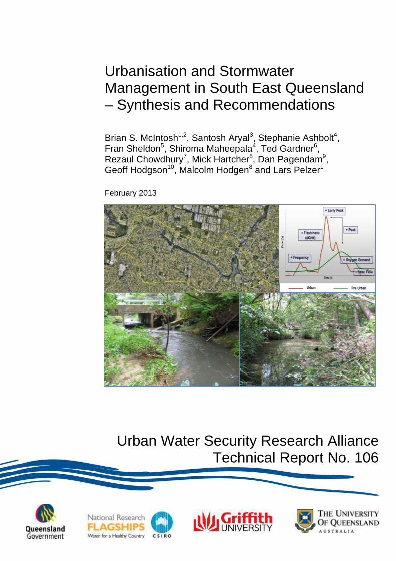
Urbanisation and Stormwater Management in South East Queensland – Synthesis and Recommendations Brian S. McIntosh1,2, Santosh Aryal3, Stephanie Ashbolt4, Fran Sheldon5, Shiroma Maheepala4, Ted Gardner6, Rezaul Chowdhury7, Mick Hartcher8, Dan Pagendam9, Geoff Hodgson10, Malcolm Hodgen8 and Lars Pelzer1
February 2013
Urban Water Security Research Alliance Technical Report No. 106
Urban Water Security Research Alliance Technical Report ISSN 1836-5566 (Online)
Urban Water Security Research Alliance Technical Report ISSN 1836-5558 (Print)
The Urban Water Security Research Alliance (UWSRA) is a $50 million partnership over five years between the
Queensland Government, CSIRO’s Water for a Healthy Country Flagship, Griffith University and The
University of Queensland. The Alliance has been formed to address South East Queensland's emerging urban
water issues with a focus on water security and recycling. The program will bring new research capacity to South
East Queensland tailored to tackling existing and anticipated future issues to inform the implementation of the
Water Strategy.
For more information about the:
UWSRA - visit http://www.urbanwateralliance.org.au/
Queensland Government - visit http://www.qld.gov.au/
Water for a Healthy Country Flagship - visit www.csiro.au/org/HealthyCountry.html
The University of Queensland - visit http://www.uq.edu.au/
Griffith University - visit http://www.griffith.edu.au/
Enquiries should be addressed to:
The Urban Water Security Research Alliance Brian McIntosh
PO Box 15087 International WaterCentre
CITY EAST QLD 4002 BRISBANE QLD 4000
Ph: 07-3247 3005 Ph: 07-3123 7766
Email: [email protected] Email: [email protected]
Authors: 1 – International WaterCentre
2 – Smart Water Research Centre, Griffith University
3 – CSIRO Land and Water, Canberra
4 – CSIRO Land and Water, Highett
5 – Australian Rivers Institute, Griffith University
6 – Central Queensland University, Noosa
7 – UAE University, Al Ain
8 – CSIRO Land and Water, Brisbane
9 – CSIRO Mathematics, Informatics and Statistics, Brisbane
10 – CSIRO Land and Water, Perth
McIntosh, B.S., Aryal, S., Ashbolt, S., Sheldon, F., Maheepala, S., Gardner, T., Chowdhury, R., Gardiner, R.,
Hartcher, M., Pagendam, D., Hodgson, G., Hodgen, M. and Pelzer, L. (2013). Urbanisation and Stormwater
Management in South East Queensland – Synthesis and Recommendations. Urban Water Security Research
Alliance Technical Report No. 106.
Copyright
© 2013 GU. To the extent permitted by law, all rights are reserved and no part of this publication covered by
copyright may be reproduced or copied in any form or by any means except with the written permission of GU.
Disclaimer
The partners in the UWSRA advise that the information contained in this publication comprises general
statements based on scientific research and does not warrant or represent the accuracy, currency and
completeness of any information or material in this publication. The reader is advised and needs to be aware that
such information may be incomplete or unable to be used in any specific situation. No action shall be made in
reliance on that information without seeking prior expert professional, scientific and technical advice. To the
extent permitted by law, UWSRA (including its Partner’s employees and consultants) excludes all liability to
any person for any consequences, including but not limited to all losses, damages, costs, expenses and any other
compensation, arising directly or indirectly from using this publication (in part or in whole) and any information
or material contained in it.
Cover Photographs:
Description: Stormwater impacts of urbanisation (aerial photo of Sunnybank, photos of Tingalpa Creek and
Stable Swamp Creek, and diagram representing hydrological changes following urbanisation).
Photographer: Richard Gardiner
© 2013 GU
Urbanisation and Stormwater Management in South East Queensland – Synthesis and Recommendations Page i
ACKNOWLEDGEMENTS
This research was undertaken as part of the South East Queensland Urban Water Security Research
Alliance, a scientific collaboration between the Queensland Government, CSIRO, The University of
Queensland and Griffith University.
Particular thanks go to everyone involved in the hydrological and ecological field work, particularly
Richard Gardiner, Michael Tonks and Ben Ferguson (all from Queensland Government DSITIA,
formerly DERM). Your tireless efforts to gather, collate and manage high quality hydrological and
water quality data have provided the work reported here with enviable underlying empirical rigour.
The support of Stewart Burn (CSIRO), Larry Little (Smart Water Research Centre) and Mark Pascoe
(International Water Centre) for the work reported here is acknowledged.

Urbanisation and Stormwater Management in South East Queensland – Synthesis and Recommendations Page ii
FOREWORD
Water is fundamental to our quality of life, to economic growth and to the environment. With its
booming economy and growing population, Australia's South East Queensland (SEQ) region faces
increasing pressure on its water resources. These pressures are compounded by the impact of climate
variability and accelerating climate change.
The Urban Water Security Research Alliance, through targeted, multidisciplinary research initiatives,
has been formed to address the region’s emerging urban water issues.
As the largest regionally focused urban water research program in Australia, the Alliance is focused on
water security and recycling, but will align research where appropriate with other water research
programs such as those of other SEQ water agencies, CSIRO’s Water for a Healthy Country National
Research Flagship, Water Quality Research Australia, eWater CRC and the Water Services
Association of Australia (WSAA).
The Alliance is a partnership between the Queensland Government, CSIRO’s Water for a Healthy
Country National Research Flagship, The University of Queensland and Griffith University. It brings
new research capacity to SEQ, tailored to tackling existing and anticipated future risks, assumptions
and uncertainties facing water supply strategy. It is a $50 million partnership over five years.
Alliance research is examining fundamental issues necessary to deliver the region's water needs,
including:
ensuring the reliability and safety of recycled water systems.
advising on infrastructure and technology for the recycling of wastewater and stormwater.
building scientific knowledge into the management of health and safety risks in the water supply
system.
increasing community confidence in the future of water supply.
This report is part of a series summarising the output from the Urban Water Security Research
Alliance. All reports and additional information about the Alliance can be found at
http://www.urbanwateralliance.org.au/about.html.
Chris Davis
Chair, Urban Water Security Research Alliance
Urbanisation and Stormwater Management in South East Queensland – Synthesis and Recommendations Page iii
CONTENTS
Acknowledgements ................................................................................................................. i
Foreword ................................................................................................................................. ii
Executive Summary ................................................................................................................ 1
1. Introduction ................................................................................................................... 3
2. The Impact of Urbanisation on Catchment Hydrology – a Model-Based Assessment ................................................................................................................... 6
2.1 Method ................................................................................................................................. 7 2.1.1 Climate and Catchment Characteristics ........................................................................... 7 2.1.2 Simulation Procedure ....................................................................................................... 8
2.2 Results ................................................................................................................................. 9 2.2.1 Baseline Simulations ........................................................................................................ 9 2.2.2 Urbanisation Scenarios .................................................................................................. 11
2.3 Discussion .......................................................................................................................... 15
3. Understanding how Urbanisation Impacts Stream Ecology in South East Queensland .................................................................................................................. 17
3.1 Impacts of Impervious Area on Ecosystem Health ............................................................ 18 3.1.1 Introduction and Aims ..................................................................................................... 18 3.1.2 Methods .......................................................................................................................... 18 3.1.3 Results ........................................................................................................................... 20 3.1.4 Conclusions .................................................................................................................... 20
3.2 Focussed Temporal Analysis ............................................................................................. 23 3.2.1 Introduction and Aims ..................................................................................................... 23 3.2.2 Hydrological Differences ................................................................................................. 23 3.2.3 Water Quality Differences ............................................................................................... 27 3.2.4 Macroinvertebrate Community Composition ................................................................... 30
3.3 Conclusions ....................................................................................................................... 36
4. An Evaluation of the SEQ Frequent Flow Approach to Urban Stormwater Management ................................................................................................................ 37
4.1 Method ............................................................................................................................... 38
4.2 Results ............................................................................................................................... 38 4.2.1 Scrubby Creek ................................................................................................................ 38 4.2.2 Upper Yuan Creek .......................................................................................................... 40 4.2.3 Tingalpa Creek ............................................................................................................... 41
4.3 Discussion .......................................................................................................................... 42 4.3.1 Hydrological Effectiveness ............................................................................................. 42 4.3.2 Ecological Effectiveness ................................................................................................. 44
5. Conclusions and Recommendations ........................................................................ 46
5.1 Develop with the Catchment in Mind ................................................................................. 47
5.2 Focus on Maintaining Winter Flows, In-Stream Habitat and Riparian Zones .................... 48
5.3 Clarify the Relative Impacts of Construction vs. Urban Impervious Area on Waterway Ecological Health .............................................................................................. 49
References ............................................................................................................................ 50
Urbanisation and Stormwater Management in South East Queensland – Synthesis and Recommendations Page iv
LIST OF FIGURES
Figure 1. Typical impacts of urbanisation on catchment hydrology and contemporary urban
stormwater management approaches to returning post-development hydrology to pre-
development hydrology (from Fletcher et al. 2013, adapted from Marsalek et al. 2007) (pre-
development indicates before urbanisation, and post-development indicates after
urbanisation). ..................................................................................................................................... 3 Figure 2. Types and locations of gauged catchments in SEQ, these catchments are grouped into
three categories - Reference indicates un-impacted catchments; Urban indicates
catchments with significant degree of urban development; WSUD indicates catchments with
a significant degree of urban development and features such as wetlands and storage
ponds for flow treatment and retention, and; Mixed indicates catchments with a combination
of reference, urban and WSUD components (from Chowdhury et al. 2012)...................................... 6 Figure 3. Flow duration curves for hourly flows for the study catchments under baseline conditions for
a common period of 2000 to 2007. The y axis is in log scale. ......................................................... 10 Figure 4. Effect of increasing TIA on flow duration curves in Scrubby Creek catchment. The y axis is in
log scale. ......................................................................................................................................... 12 Figure 5. Modelled mean, max and 90 percentile hourly flow rate for different total impervious areas in
Scrubby Creek catchment. The y axis is in log scale. ..................................................................... 12 Figure 6. Effects of total impervious area on (left) high and (right) low flow spells in Scrubby Creek
catchment. ....................................................................................................................................... 12 Figure 7. Effect of increasing TIA on flow duration curves in Upper Yuan Creek catchment. ......................... 13 Figure 8. Modelled mean, max and 90 percentile hourly flow rate for different total impervious areas in
Upper Yuan Creek catchment. The y axis is in log scale. ................................................................ 13 Figure 9. Effects of total impervious area on (left) high and (right) low flow spells in Upper Yuan Creek
catchment. ....................................................................................................................................... 14 Figure 10. Effect of increasing TIA on flow duration curves in Tingalpa Creek catchment. .............................. 14 Figure 11. Modelled mean, max and 90 percentile hourly flow rate for different total impervious areas in
Tingalpa Creek catchment. The y axis is in log scale. ..................................................................... 15 Figure 12. Effects of total impervious area on (a) high and (b) low flow spells in Tingalpa Creek
catchment. ....................................................................................................................................... 15 Figure 13. Conceptual model of the impacts on instream aquatic invertebrates caused by urbanisation
(from Sheldon et al. 2012a). ............................................................................................................ 17 Figure 14. Landscape weighting metrics from Peterson et al (2011). ............................................................... 19 Figure 15. Relationships between total catchment urban area (% area, x-axis) and four urban area
metrics (weighted % area, y-axis) across the 36 most urbanised EHMP catchments. .................... 21 Figure 16. Relationships between total catchment urban area (% area, x-axis) and lumped (non-
weighted) lumped TIA area (m2, y-axis) across the 9 most urbanised EHMP catchments. ............ 22 Figure 17. Mean number of flow rises (±SE) for months by site. ...................................................................... 24 Figure 18. Mean daily flow (±SE) for months by site (ML/day). ........................................................................ 25 Figure 19. Mean magnitude of pulse rise (ML/day) (±SE) for months by site. .................................................. 25 Figure 20. Mean (±SE) magnitude of falling limb (ML/day). .............................................................................. 26 Figure 21. Mean (±SE) minimum flow by month and site (ML/day). ................................................................. 26 Figure 22. Mean daily dissolved oxygen (mg/L) levels across all three sites grouped by season
(Autumn: March-May; Winter: June-August; Spring: September-November; Summer:
December-February). ...................................................................................................................... 28 Figure 23. Mean daily dissolved oxygen range (mg/L) (± SE) across all three sites for the period of
record. ............................................................................................................................................. 28 Figure 24. Maximum daily temperature (oC) (± SE) across all three sites for the period of record................... 29 Figure 25. Mean daily temperature range (oC) (± SE) across all three sites for the period of record. .............. 29 Figure 26. Mean daily conductivity (S) (± SE) across all three sites for the period of record. ......................... 30 Figure 27. Species richness box plots (showing minimum, first quartile, median, third quartile, and
maximum values) for the two sites (Tingalpa Creek – forested and Stable Swamp Creek –
Urban) for each habitat type. ........................................................................................................... 34 Figure 28. Mean (± SE) of species richness for the ‘pool’ habitat in the two streams across the
sampling months. ............................................................................................................................ 34
Urbanisation and Stormwater Management in South East Queensland – Synthesis and Recommendations Page v
Figure 29. Mean (± SE) of species richness for the ‘riffle’ habitat in the two streams across the
sampling months. ............................................................................................................................ 35 Figure 30. Comparative proportion of pools and riffles in 1km sections of urban and forested streams in
the Brisbane area. ........................................................................................................................... 35 Figure 31. Effect of flow capture on flow duration curve for increasing TIA for Scrubby Creek. Plots for
only 20, 50 and 70 percent TIA are shown for clarity. ..................................................................... 39 Figure 32. Effect of flow capture implemented as frequent flow management option (FFMO) on top 90
percentile flow in the Scrubby Creek catchment. ............................................................................. 39 Figure 33. Effect of flow capture on the (left) high flow and (right) low flow duration in Scrubby Creek
catchment. ....................................................................................................................................... 39 Figure 34. Effect of flow capture on flow duration curve for increasing TIA for Upper Yuan Creek. Plots
for only 20, 50 and 70 percent TIA are shown for clarity. ................................................................ 40 Figure 35. Effect of flow capture implemented as frequent flow management option (FFMO) on top 90
percentile flow in the Upper Yuan Creek catchment. ....................................................................... 40 Figure 36. Effect of flow capture on the (left) high flow and (right) low flow duration in Upper Yuan
Creek catchment. ............................................................................................................................ 41 Figure 37. Effect of flow capture on flow duration curve for increasing TIA for Tingalpa Creek. Plots for
only 20, 50 and 70 percent TIA are shown for clarity. ..................................................................... 41 Figure 38. Effect of flow capture implemented as frequent flow management option (FFMO) on top 90
percentile flow in the Tingalpa Creek catchment. ............................................................................ 42 Figure 39. Effect of flow capture on the (left) high flow and (right) low flow duration in Tingalpa Creek
catchment. ....................................................................................................................................... 42
LIST OF TABLES
Table 1. Area, topography, land use and key features of the eight study catchments (TIA – total
impervious area, TOC – Time of concentration, Slope – average slope). ......................................... 8 Table 2. Details of rainfall data and weather stations used to run baseline scenarios (AWS =
automatic weather station). ............................................................................................................... 9 Table 3. Flow statistics from baseline scenarios. .......................................................................................... 10 Table 4. Description of EHMP ecological response variables. ...................................................................... 19 Table 5. Mean (±SE) for a range of diversity measures for each site by sampled month for riffle
habitats only. ................................................................................................................................... 31 Table 6. Mean (±SE) for a range of diversity measures for each site by sampled month for pool
habitats only. ................................................................................................................................... 32
Urbanisation and Stormwater Management in South East Queensland – Synthesis and Recommendations Page 1
EXECUTIVE SUMMARY
The ecological health of waterways is generally known to be impacted by the hydrologic and water
quality changes which occur as a consequence of urbanisation. The aims of the research reported here
were: to develop detailed characterisation of the hydrological, water quality and ecological impacts of
urbanisation in SEQ across a range of catchments; to tease apart the likely causes of ecological
impacts; and, having done so, to make a set of recommendations about how urbanisation might be
managed differently to help avoid waterway ecological degradation. SEQ has a sub-tropical climate
and the existing literature on the impacts of urbanisation has been developed mostly focussed on
temperate climate conditions. This report provides a synthesis of the range of research results
generated by the project and a set of management and research recommendations developed in critical
response to the results.
Twelve catchments in the Brisbane and Gold Coast areas of SEQ were gauged hydrologically for three
years to yield a sufficient quantity and quality of flow and rainfall data to develop reliable catchment
models using the Stormwater Management Model (SWMM) platform. In addition, the total
impervious area (TIA) for those catchments was determined from aerial photographs. SWMM models
were successfully developed for eight of those catchments using a generic algorithm automatic
parameterisation approach. At the same time as flow data was gathered, water quality data on pH,
temperature, conductivity and turbidity was gathered for each catchment using Sonde instrumentation
to allow the impacts of water quality change on ecological health to be assessed.
These models were used to assess how hydrology changes with urbanisation intensity and pattern.
First of all, a set of baseline simulations were run using long time-series hourly rainfall data for the
catchments to investigate how increasing TIA impacts on catchment hydrology. Next, three pre-
development (no urbanisation) catchment models were used to simulate, using long time-series hourly
rainfall, the impacts of increasing levels of urbanisation as characterised by per cent TIA (%TIA).
From the modelling results, urbanisation is clearly associated with changes in hydrology, but the
changes are complex. Whilst there are some generalities (increases in high flow condition duration,
increases in mean flow and 90th percentile flow, increases in the frequency and rate of runoff event
rise), the hydrological impact of urbanisation depends on catchment characteristics, including size,
slope, time of concentration (ToC), sub-catchment sizes and distributions, and on the pattern of
urbanisation itself across sub-catchments and the catchment as a whole. The same urbanisation pattern
can exert a qualitatively different impact hydrologically, depending on the composition of the whole
catchment in terms of sub-catchments. Maximum hourly flows appear not to be impacted by
urbanisation, but 90th percentile hourly flows and mean hourly flows are impacted, both increasing
with urbanisation. The number of runoff events increases with urbanisation and the size of the rise and
fall in flow with each event also increases with urbanisation.
The proportion of time spent under high flow conditions tends to increase with urbanisation for any
given catchment, but not necessarily so – there can be some catchment specific decreases in high flow
spell duration under urbanisation, depending on sub-catchment characteristics. The mean of high flow
spells may increase, but not necessarily so. The proportion of time spent under low flow conditions
tends to decrease with urbanisation, probably as a consequence of the streams studied being ephemeral
in their pre-development state rather than strongly base flow supported and perennial.
To understand how urbanisation affects the ecology of urban streams and waterways, a conceptual
model was developed to articulate the range of potential mechanisms, and these mechanisms were
then investigated through a mixture of means, by way of: statistically analysing the relationships
between urban land use (particularly imperviousness) and Ecosystem Health Monitoring Program
(EHMP) score and indicators; characterising macroinvertebrate assemblages present in three selected
case study sites (one reference and two urban) and how these assemblages vary between summer and
winter seasons or high and low flow conditions; and relating the assemblage data to hydrological and
water quality variables in the sites concerned.
Urbanisation and Stormwater Management in South East Queensland – Synthesis and Recommendations Page 2
The research reported here clearly indicates that there are negative aquatic ecological impacts
associated with urbanisation in SEQ. In particular, the EHMP analysis demonstrates that urbanisation
(as a lumped land use category) is associated with decreases in macroinvertebrate richness, and
increase in the proportion of alien fish species observed. TIA, either lumped or weighted to mimic the
effect of directly connected impervious area (DCIA), was not observed to exert a strong impact on any
ecological variables.
The ecological results tend to indicate that the hydrological changes following urbanisation are not
significant degrading factors in themselves, rather, the water quality variables, particularly temperature
range, are more likely to be important. The association of lumped urban land use with ecological
impact and the simultaneous lack of ecological impact associated with IA (TIA or proxied DCIA)
raise the question as to whether the process of urbanisation, i.e. the process of construction, is the
primary source of ecologically degrading waterway impact in SEQ, rather than the on-going impact of
impervious area runoff flows.
Whilst urban and pre-development streams had similar levels of macroinvertebrate species richness
and diversity, and similar distributions of habitat availability (riffle and pool proportions), there were
significant differences over time (seasonally) within each stream type and between each stream type in
relation to species composition. Pool species composition in both urban and pre-development streams
was found to be stable over time, i.e. not affected by higher summer or lower winter flows.
Conversely, riffle species composition in the urban stream was found to vary significantly over time,
with lower diversity in the lower flow winter months, suggesting the importance of water quality
changes rather than flow changes as a driver of assemblage change.
As with hydrological impact, the mechanisms of ecological change from urbanisation are complicated
and based partly on catchment specific features, e.g., the winter flow supporting upstream wetlands in
Stable Swamp Creek and the ecologically locally devastating iron floc problems at Blunder Creek.
Finally, the evaluation of the Qld frequent flow management objectives (FFMOs) as an ecologically
oriented flow management policy instrument designed to avoid the ecological impacts associated with
urbanisation, suggests that they will bring catchment hydrographs back towards their pre-development
profile, but are insufficiently strong. The FFMOs will have an effect which is partly dependent on
catchment characteristics, the distribution and sizes of sub-catchments and the spatial pattern of
urbanisation.
Urbanisation and Stormwater Management in South East Queensland – Synthesis and Recommendations Page 3
1. INTRODUCTION
The process of urbanisation is relentlessly transforming the social and economic geography of almost
every country in the world. More than 50% of the world’s seven billion people live in cities already
and this figure is expected by the United Nations to rise to over 70% by 2050, when the total global
population will be just under nine billion people. Driven by absolute growth in total population, and
both absolute and relative growth in the populations of urban areas, the physical footprint of towns and
cities is expanding. This means the expansion of housing, roads, business, industrial and retail land
uses into natural and agricultural landscapes around towns and cities, typically involving vegetation
removal or thinning, changes to riparian vegetation, the construction of extensive impervious area in
the form of roads, buildings and paths, and sometimes the deliberate modification of stream channels.
The expansion of imperviousness across catchments during and as a consequence of urbanisation is
well recognised as a primary driver of hydrological change (Burns et al. 2012), which itself is a key
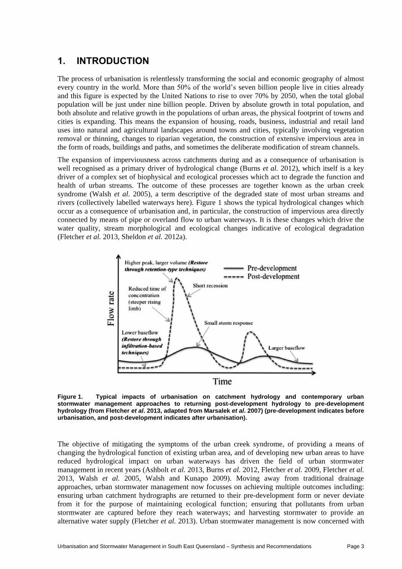
driver of a complex set of biophysical and ecological processes which act to degrade the function and
health of urban streams. The outcome of these processes are together known as the urban creek
syndrome (Walsh et al. 2005), a term descriptive of the degraded state of most urban streams and
rivers (collectively labelled waterways here). Figure 1 shows the typical hydrological changes which
occur as a consequence of urbanisation and, in particular, the construction of impervious area directly
connected by means of pipe or overland flow to urban waterways. It is these changes which drive the
water quality, stream morphological and ecological changes indicative of ecological degradation
(Fletcher et al. 2013, Sheldon et al. 2012a).
Figure 1. Typical impacts of urbanisation on catchment hydrology and contemporary urban stormwater management approaches to returning post-development hydrology to pre-development hydrology (from Fletcher et al. 2013, adapted from Marsalek et al. 2007) (pre-development indicates before urbanisation, and post-development indicates after urbanisation).
The objective of mitigating the symptoms of the urban creek syndrome, of providing a means of
changing the hydrological function of existing urban area, and of developing new urban areas to have
reduced hydrological impact on urban waterways has driven the field of urban stormwater
management in recent years (Ashbolt et al. 2013, Burns et al. 2012, Fletcher et al. 2009, Fletcher et al.
2013, Walsh et al. 2005, Walsh and Kunapo 2009). Moving away from traditional drainage
approaches, urban stormwater management now focusses on achieving multiple outcomes including:
ensuring urban catchment hydrographs are returned to their pre-development form or never deviate
from it for the purpose of maintaining ecological function; ensuring that pollutants from urban
stormwater are captured before they reach waterways; and harvesting stormwater to provide an
alternative water supply (Fletcher et al. 2013). Urban stormwater management is now concerned with
Urbanisation and Stormwater Management in South East Queensland – Synthesis and Recommendations Page 4
a combination of flood prevention, ecological restoration and enhancement, and water supply. This
represents a significant progression from a sole focus on draining urban catchments as quickly as
possible, a strategy which is now recognised as resulting in increased waterway and coastal pollutant
loads, and the hydraulic scouring and degradation of stream morphology, in-stream habitat and animal
populations (Burns et al. 2012, Walsh et al. 2005).
The story of population growth, urbanisation and urban stream degradation is also to be found in
South East Queensland (SEQ). Here, as with almost everywhere, processes of urbanisation are
working apace, with the major urban centres of the region having grown substantially between 2001
and 2010, e.g., Brisbane’s population having grown by 19%, the population of the Gold Coast by 27%,
Ipswich by 34% and the Sunshine Coast by 34%, and the region as a whole by 26% (OESR 2011a).
This growth is expected to slow over the period 2011-2056, but nevertheless, the population of the
whole State is expected to almost double by 2056, with most of that growth anticipated to occur in
existing urban areas (OESR 2011b).
Quite how expected population growth will translate into expansion of urban areas is not yet known or
decided. There are pressures to densify urban form, although one outcome of densification processes
in urban SEQ has been characterised as the ‘death of the Australian backyard’ (Hall 2010). Under such
a situation, lots are subdivided, houses built closer to the perimeter than ever before to maximise house
size and, as a consequence, lawns disappear or shrink dramatically. Such a process increases the total
impervious area in a catchment and risks exaggerating the differences between pre- and post-
development hydrology in urban catchments. There are also pressures to expand through the
construction of significant new housing developments such as Ripley Valley near Ipswich. Expansion
of total urban area and the urbanisation of previously undeveloped land will inevitably have
hydrological and ecological impacts, the question is to what degree? How can the hydrological and
consequently ecological impacts of stormwater generated by the increase of urban area, and
particularly impervious urban area, be mitigated for the purposes of maintaining ecological health and
enhancing urban liveability?
To answer these questions requires a good knowledge of the relationships between urbanisation,
hydrological change and ecological impact, and this in turn requires good knowledge of local
catchments and ecologies. Much of the existing research into urban stormwater management has been
conducted on temperate catchments, often in Melbourne in Australia (e.g. Burns et al. 2012, Fletcher
et al. 2008, Walsh and Kunapo 2009). SEQ is sub-tropical and consequently qualitatively different
climatically – wetter, hotter summers with frequent intense rainfall storms, and drier, warmer winters.
Flashy catchment runoff and stream ephemerality are normal in SEQ – whether in pre-development or
urbanised situations. Do these climatic differences mean that urbanisation has a different impact on
urban catchment hydrology than in temperate climates? Do these differences mean that the consequent
impacts on ecology from hydrological change are different to those typically observed in temperate
climates? What are the implications of any observed differences on the way in which urban
stormwater should be managed in existing and new urban areas across SEQ?
Little academic literature is available which focusses on urban stormwater management within the
climate and conditions of SEQ, or Queensland more generally. Where research has been undertaken,
peer reviewed and published, analysis has been based on regionally specific climate data but without
catchment specific hydrological gauging (e.g. Fletcher et al. 2007). As a consequence, it is difficult to
assess how representative the results are of the kinds of catchment, climate and ecological conditions
found in SEQ. Having said that, the need to manage the hydrological impacts of urbanisation is well
recognised in Queensland, with policies in place to mitigate changes in flow regime arising as a
consequence of increased impervious area – notably the state wide application of frequent flow
management objectives (FFMOs) as an instrument to prevent or limit the extent to which urban
development changes catchment hydrology away from pre-development conditions (DIP 2009).
The aim of this report is to describe the outcomes of a UWSRA funded research project into
stormwater management in SEQ, with a particular focus on eco-hydrology, that is to say, the
relationships between urban area and the ecological consequences of changed hydrology. In particular,
the aim of this report is to synthesise the outcomes of the project to provide a set of recommendations
to improve the eco-hydrological outcomes of managing stormwater in urban SEQ. The specific
questions to be addressed by this report are as follows:

Urbanisation and Stormwater Management in South East Queensland – Synthesis and Recommendations Page 5
1. How does the imperviousness of urban areas influence the hydrology and ecology of streams in
South East Queensland?
2. How effective is the current frequent flow management objective approach to managing the
hydrological and ecological impacts of urbanisation in South East Queensland?
3. What recommendations for action and what gaps in knowledge are suggested by the research in
relation to urban stormwater management in South East Queensland?
This report is accompanied by two more detailed reports already published – one describing the
technical aspects of the catchment modelling approach used (Chowdhury et al. 2012) and the other
describing the findings of the urban creek ecology focussed sub-project which examined in detail three
urban streams around Brisbane (Sheldon et al. 2012a). The aim of this report is to bring together
project results, to synthesise and make recommendations. This report will repeat some of the results
found in Chowdhury et al. (2012) and Sheldon et al. (2012a) for the purpose of creating this synthesis,
but will not provide a full account of those results nor the methods employed to generate them. For
this, the interested reader is referred to the original reports. The results of applying the catchment
modelling developed are not documented in Chowdhury et al. (2012) and so will be documented more
fully here.
The interested reader is also directed towards the results of the frequent flow management approach
evaluation for Tingalpa and Upper Yuan creeks which are presented, respectively, in Ashbolt et al.
(2012) and Ashbolt et al. (2013). A separate report into stormwater harvesting strategies assessing
variation in yields from different collection and storage options along a gradient of decentralised to
centralised, under a range of urban densities, and the potential ecological implications is also
forthcoming.
The structure of the report will be as follows.
First, following this introduction, the results of the hydrological modelling assessment of the
impacts of urbanisation will be presented and discussed. This will partly answer question (1)
above.
Second, the results from two pieces of urban stream ecology research will be presented
regarding the mechanisms of impact on waterway ecology from different intensities (degrees of
imperviousness) of urban development. This will complete the answer to question (1) above.
Third, the results from an assessment of the effect of applying the current Queensland urban
stormwater frequent flow management objectives (FFMOs) to different urbanisation scenarios
will be presented and discussed in relation to their ability to: (i) maintain catchment hydrology
in pre-development conditions; and (ii) their consequent ability to prevent ecological
degradation. This will answer question (2) above.
Finally, the results and discussion from the previous three sections will be presented in the form
of recommendations for action and a characterisation of knowledge gaps. This will answer
question (3) above.
Urbanisation and Stormwater Management in South East Queensland – Synthesis and Recommendations Page 6
2. THE IMPACT OF URBANISATION ON CATCHMENT HYDROLOGY – A MODEL-BASED ASSESSMENT
Hydrologic modelling is a well-accepted means of investigating and understanding urban stormwater
hydrology (Fletcher et al. 2013). Such models enable the exploration of catchment response to rainfall
over long time-periods based on shorter time-period flow data. They also enable runoff changes in
response to rainfall changes to be investigated and the evaluation of catchment management options to
be undertaken without the need for physical intervention. Needless to say, the quality of model outputs
is critically dependent on the quality, and quantity of input data in terms of monitored flows.
Twelve urban and pre-development streams around Brisbane and the hinterland of the Gold Coast
were hydrologically gauged, cross-sectioned and continuous flow monitored for three years to provide
high quality, fine detail information on stream flow. This data was used to calibrate and then validate a
set of Stormwater Management Model (SWMM) hydrologic models, one for each catchment, which
were then used to characterise the hydrology of each catchment using long time-series, hourly rainfall.
In addition, the same twelve streams were instrumented for standard water quality measurements (pH,
DO, turbidity etc) using SONDE systems.
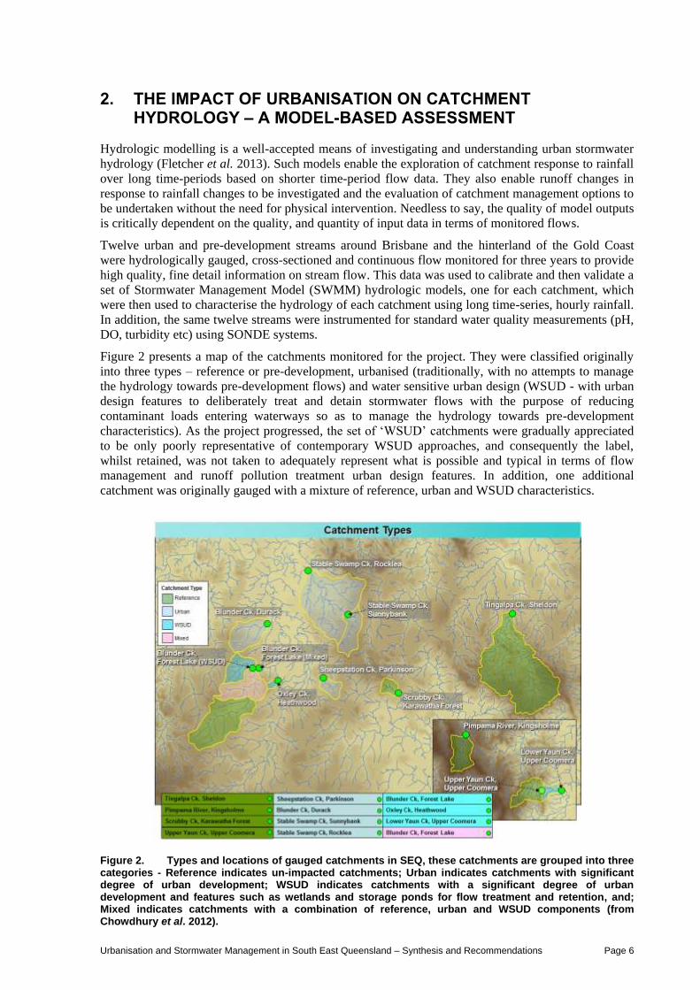
Figure 2 presents a map of the catchments monitored for the project. They were classified originally
into three types – reference or pre-development, urbanised (traditionally, with no attempts to manage
the hydrology towards pre-development flows) and water sensitive urban design (WSUD - with urban
design features to deliberately treat and detain stormwater flows with the purpose of reducing
contaminant loads entering waterways so as to manage the hydrology towards pre-development
characteristics). As the project progressed, the set of ‘WSUD’ catchments were gradually appreciated
to be only poorly representative of contemporary WSUD approaches, and consequently the label,
whilst retained, was not taken to adequately represent what is possible and typical in terms of flow
management and runoff pollution treatment urban design features. In addition, one additional
catchment was originally gauged with a mixture of reference, urban and WSUD characteristics.
Figure 2. Types and locations of gauged catchments in SEQ, these catchments are grouped into three categories - Reference indicates un-impacted catchments; Urban indicates catchments with significant degree of urban development; WSUD indicates catchments with a significant degree of urban development and features such as wetlands and storage ponds for flow treatment and retention, and; Mixed indicates catchments with a combination of reference, urban and WSUD components (from Chowdhury et al. 2012).
Urbanisation and Stormwater Management in South East Queensland – Synthesis and Recommendations Page 7
Chowdhury et al. (2012) describe the hydrologic and water quality instrumentation employed, and the
model development process including calibration (automatically using a generic algorithm based
system) and validation. Chowdhury et al. (2012) also describe the aerial image analysis method
employed to characterise each catchment in terms of percentage total impervious area (%TIA). %TIA
was used for reasons of (i) simplicity and (ii) a lack of reliable or complete information on how
impervious areas connected directly to streams in Brisbane (the information was sought early in the
project). In section 4, an assessment of the relationships between directly connected impervious area
(IA) and components of ecosystem health will be presented to provide insight into the extent to which
hydraulic connectedness is an important element of the influence of imperviousness on waterway
ecology in SEQ.
The set of SWMM models developed were used to: (i) tease apart the relationships between catchment
%TIA, land cover (reference, urban, WSUD) and hydrological characteristics, particularly high and
low flows due to their potential ecological relevance (see Kennard et al. 2010 for an assessment of
ecologically relevant flow components in Australian rivers); and (ii) evaluate the effectiveness of the
current FFMO approach to managing urban stormwater flows. This section presents the results of the
first use, to tease apart the relationships between %TIA, land cover and hydrology. The results of
investigation into the ecological consequences of changed catchment hydrology under conditions of
urbanisation (higher %TIA particularly) are documented in section 3, whilst the results of the FFMO
evaluation can be found in section 4.
This section will begin by way of providing a description of the region climatically, greater detail
regarding the catchments studied, and a description of the simulation procedure employed.
2.1 Method
The reader is referred to Chowdhury et al. 2012 for methodological detail relating to model
development, calibration and validation. Here we will describe the catchments modelled in more
detail, the climate of the area and the simulation procedure.
2.1.1 Climate and Catchment Characteristics
The SEQ region experiences a sub-tropical climate with average annual rainfall and potential
evapotranspiration of the area are 1150 mm and about 1450 mm respectively (BoM, 2012). The
rainfall is seasonal with heaviest falls occurring during southern hemisphere summer. Runoff from the
SEQ urban area varies between 240 and 750 gigalitre/year (GL/y), of which about half is required to
maintain the environmental flow requirements in the lower reaches of SEQ river systems (Chowdhury
et al., 2012). The mean daily temperature in this area ranges from 7oC to 30oC with highest
temperature going up to 43oC (at Archerfield Airport).
Following validation, a decision was made to use only eight of the 12 SWMM catchment models. The
others were not sufficiently well validated, either because an insufficient length of flow data was
available for the variability in runoff conditions, or because there was knowledge that the catchments
had developed since the TIA aerial image analysis had been undertaken, and were now behaving
differently as a consequence. To use the remaining four models would require additional hydrological
monitoring to lengthen the time series of flow data.
All eight streams are ephemeral with different degrees of intermittency. The time of concentration (tc)
computed using the Bransby-Williams formula by Chowdhury et al. (2012) shows that the tc ranges
from 0.8 to 9 hours, suggesting less than daily but more than hourly catchment response times.
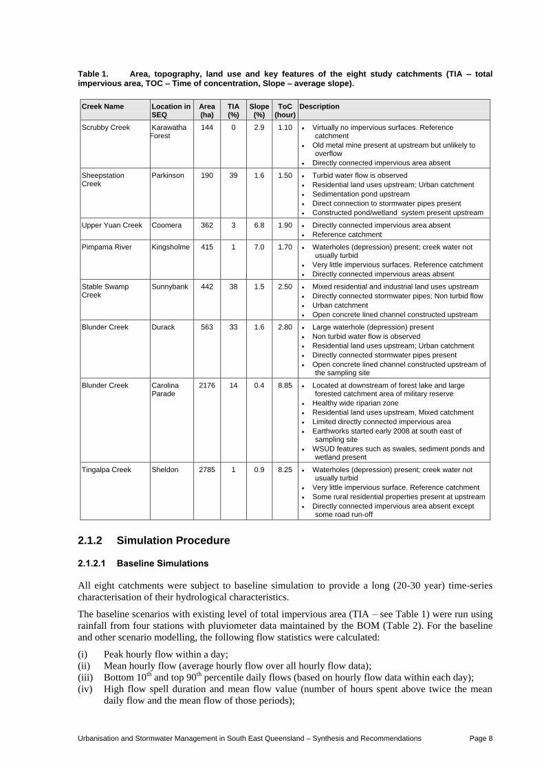
Table 1 describes the catchments modelled in terms of hydrologically relevant characteristics (also see
Figure 2 for their locations relatively). The existing TIA ranged from 0 to 38%. As described before,
the catchments have four different characteristic land uses: (i) Reference - undisturbed and forested;
(ii) Urban - with urban development; (iii) WSUD -development with WSUD features; and (iv) Mixed
– a combination of all three.
Urbanisation and Stormwater Management in South East Queensland – Synthesis and Recommendations Page 8
Table 1. Area, topography, land use and key features of the eight study catchments (TIA – total impervious area, TOC – Time of concentration, Slope – average slope).
Creek Name Location in SEQ
Area (ha)
TIA (%)
Slope (%)
ToC (hour)
Description
Scrubby Creek Karawatha Forest
144 0 2.9 1.10 Virtually no impervious surfaces. Reference catchment
Old metal mine present at upstream but unlikely to overflow
Directly connected impervious area absent
Sheepstation Creek
Parkinson 190 39 1.6 1.50 Turbid water flow is observed
Residential land uses upstream; Urban catchment
Sedimentation pond upstream
Direct connection to stormwater pipes present
Constructed pond/wetland system present upstream
Upper Yuan Creek Coomera 362 3 6.8 1.90 Directly connected impervious area absent
Reference catchment
Pimpama River Kingsholme 415 1 7.0 1.70 Waterholes (depression) present; creek water not usually turbid
Very little impervious surfaces. Reference catchment
Directly connected impervious areas absent
Stable Swamp Creek
Sunnybank 442 38 1.5 2.50 Mixed residential and industrial land uses upstream
Directly connected stormwater pipes; Non turbid flow
Urban catchment
Open concrete lined channel constructed upstream
Blunder Creek Durack 563 33 1.6 2.80 Large waterhole (depression) present
Non turbid water flow is observed
Residential land uses upstream; Urban catchment
Directly connected stormwater pipes present
Open concrete lined channel constructed upstream of the sampling site
Blunder Creek Carolina Parade
2176 14 0.4 8.85 Located at downstream of forest lake and large forested catchment area of military reserve
Healthy wide riparian zone
Residential land uses upstream, Mixed catchment
Limited directly connected impervious area
Earthworks started early 2008 at south east of sampling site
WSUD features such as swales, sediment ponds and wetland present
Tingalpa Creek Sheldon 2785 1 0.9 8.25 Waterholes (depression) present; creek water not usually turbid
Very little impervious surface. Reference catchment
Some rural residential properties present at upstream
Directly connected impervious area absent except some road run-off
2.1.2 Simulation Procedure
2.1.2.1 Baseline Simulations
All eight catchments were subject to baseline simulation to provide a long (20-30 year) time-series
characterisation of their hydrological characteristics.
The baseline scenarios with existing level of total impervious area (TIA – see Table 1) were run using
rainfall from four stations with pluviometer data maintained by the BOM (Table 2). For the baseline
and other scenario modelling, the following flow statistics were calculated:
(i) Peak hourly flow within a day;
(ii) Mean hourly flow (average hourly flow over all hourly flow data);
(iii) Bottom 10th and top 90th percentile daily flows (based on hourly flow data within each day);
(iv) High flow spell duration and mean flow value (number of hours spent above twice the mean
daily flow and the mean flow of those periods);
Urbanisation and Stormwater Management in South East Queensland – Synthesis and Recommendations Page 9
(v) Low flow spell duration and mean flow (number of hours spent below half the mean daily flow
and the mean flow of those periods); and
(vi) The flow duration curves (FDC) for each of the TIA scenarios with and without runoff capture
were also prepared.
Table 2. Details of rainfall data and weather stations used to run baseline scenarios (AWS = automatic weather station).
Stations Data Length Used by Catchments
Archerfield AWS 1994 - 2012 Blunder Creek at Carolina Pde, Blunder Creek at Durack, Stable Swamp Creek
Oxenford Weir Alert 2000 - 2011 Pimpama, Upper Yuan Creek
Shailer Park 1989 -2007 Tingalpa
Stretton Alert 1993-2011 Sheepstation, Scrubby Creek
2.1.2.2 Urbanisation Scenarios
Three of the reference catchments were selected for assessment in relation to the impacts of
urbanisation – Tingalpa, Scrubby Creek and Upper Yuan. The rationale being that their pre-
development hydrographs are known by means of direct observation (monitoring) and extrapolation
(long time-series rainfall driven simulation using models calibrated and validated against monitored
flow data). This means that pre-development hydrographs do not need to be generated by artificially
decreasing %TIA to zero, an activity which creates hydrographs of unknown certainty. What is known
is that the process of urbanisation is likely to impact stream morphology, and so, taking a model of an
already urbanised catchment and generating the pre-development hydrograph without representing
what the pre-development (and totally unknown) stream morphology would have been leaves the
reliability of the generated pre-development hydrograph uncertain. There is greater reliability in
starting from an empirically known pre-development condition and assessing the progressive impact
of increasing urbanisation, although uncertainty still remains.
A range of urbanisation scenarios were modelled, represented by a change in the %TIA of the sub-
catchments. These scenarios ranged from the current level of urbanisation (typically zero or a few
percent TIA), up to 70% impervious area, representing a high degree of urbanisation. Urbanisation
was assumed to commence in the middle portion of each catchment, up to a sub-catchment
imperviousness maximum of 55% (as typical processes of urbanisation tend not to entirely cover a
catchment), then to extend to the lower, followed by upper portions of the catchment to the total
impervious area required to reach a particular %TIA value. Scenarios of 60% and 70% impervious
were equally spread across sub-catchments.
The same flow metrics were calculated as for the baseline simulations, yielding two sets of results: a
set of flow metrics representing the hydrology of eight catchments spread across a disturbance
gradient from 0% TIA to over 40% TIA; and three sets of flow metrics representing the hydrological
impact of urbanising three of the reference catchments studied.
2.2 Results
2.2.1 Baseline Simulations
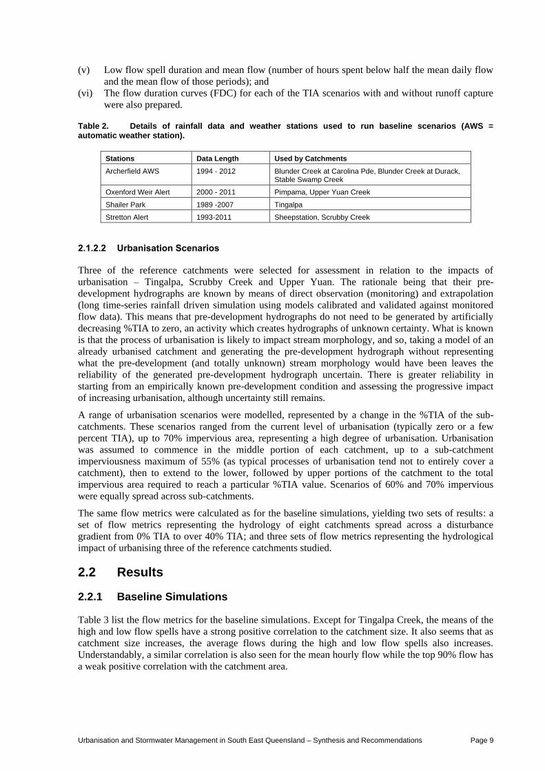
Table 3 list the flow metrics for the baseline simulations. Except for Tingalpa Creek, the means of the
high and low flow spells have a strong positive correlation to the catchment size. It also seems that as
catchment size increases, the average flows during the high and low flow spells also increases.
Understandably, a similar correlation is also seen for the mean hourly flow while the top 90% flow has
a weak positive correlation with the catchment area.
Urbanisation and Stormwater Management in South East Queensland – Synthesis and Recommendations Page 10
Table 3. Flow statistics from baseline scenarios.
Catchments Area (ha)
% TIA
Mean Hourly Flow (m3/s)
90th Percentile of Hourly Flow
(m3/s)
High Flow Spell
Duration (% of record)
Mean Flow of High
Flow Spells (m3/s)
Low Flow Spell
Duration (% of record)
Mean Flow of Low Flow
Spells (m3/s)
Scrubby Creek 144 0 0.0022 0.0 0.3 0.69 99.6 1.41E-06
Sheepstation Creek
190 39 0.029 0.010 5.6 0.49 91.1 3.88E-04
Upper Yuan Creek
362 3 0.020 0.0011 3.3 0.58 93.8 2.03E-04
Pimpama River 415 1 0.030 0.0 3.3 0.91 95.8 1.54E-04
Stable Swamp Creek
442 38 0.048 0.0055 4.6 1.01 93.0 5.19E-04
Blunder Creek at Durack
563 33 0.059 0.00060 3.6 1.61 94.7 3.41E-04
Blunder Creek at Carolina Pde
2176 14 0.11 0.013 4.3 2.52 93.4 1.47E-03
Tingalpa Creek 2785 1 0.12 0.19 7.9 1.18 74.4 1.08E-02
It is noted that, as these catchments have different existing impervious areas, different spatial
distributions of existing impervious areas, and thus different runoff generation mechanisms, an areal
normalisation would not be meaningful for the comparison of unit catchment flows.
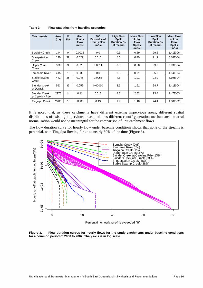
The flow duration curve for hourly flow under baseline conditions shows that none of the streams is
perennial, with Tingalpa flowing for up to nearly 80% of the time (Figure 3).
Figure 3. Flow duration curves for hourly flows for the study catchments under baseline conditions for a common period of 2000 to 2007. The y axis is in log scale.
0 20 40 60 80
1e
-05
1e
-03
1e
-01
1e
+0
1
Percent time hourly runoff is exceeded (%)
Ho
url
y r
un
off a
t ca
tch
me
nt o
utle
t (m
^3
/s)
Scrubby Creek (0%) Pimpama River (0%)Tingalpa Creek (1%)Upper Yaun Creek (3%)Blunder Creek at Carolina Pde (13%)Blunder Creek at Durack (33%)Sheepstation Creek (36%)Stable Swamp Creek (38%)
Urbanisation and Stormwater Management in South East Queensland – Synthesis and Recommendations Page 11
Teasing apart the relationships between %TIA and the flow metrics can be done by means of
examining the relationships within catchments of broadly equivalent size:
Small – Scrubby Creek (144 ha) and Sheepstation Creek (190 ha).
Medium – Upper Yuan (362 ha), Pimpama (415 ha), Stable Swamp Creek (442 ha), Blunder
Creek at Durack (563 ha).
Large – Blunder Creek at Carolina Parade (2176 ha) and Tingalpa (2785 ha).
Within each of these classes, we can see from Table 3 that the following patterns hold as %TIA
increases:
Small – mean hourly flow increases; 90th percentile of the hourly flow increases; high flow spell
mean flows increase; the proportion of time spent under high flow conditions increases; but that
the mean of low flow spell flows increases and the proportion of time spent under low flow
conditions decreases. The low flow results here run counter to the normal expected consequence
of urbanising, which is to reduce base-flow and consequently to reduce low flows (Fletcher et
al. 2013).
Medium - mean hourly flow increases; 90th percentile of the hourly flow increases sometimes
(Stable Swamp Creek) but not always (Blunder Creek at Durack has a lower 90th percentile than
the Upper Yuan); high flow spell mean flows increase, and the proportion of time spent under
high flow conditions increases but not by much; that the mean of low flow spell flows increases,
but the proportion of time spent under low flow conditions does not appear related to %TIA
(e.g. Stable Swamp Creek, 38% TIA, and Blunder Creek at Durack, 33% TIA, spend a lower
proportion of time in low flow conditions than Pimpama Creek at 1% TIA).
Large - mean hourly flow does not change (much); 90th percentile of the hourly flow is lower;
high flow spell mean flows increase, but the proportion of time spent under high flow
conditions decreases (so the pre-development hydrograph is characterised by more frequent
high flow conditions but of a lower mean high flow); that the mean of low flow spell flows
decreases, and the proportion of time spent under low flow conditions increases (as would be
expected with decreased baseflow).
Of course, these results and potential relationships represent a small sample of catchments, and
consequently are subject to the influence of both measured and unmeasured catchment specific
characteristics (soil, slope, distribution of TIA and other land uses).
2.2.2 Urbanisation Scenarios
The results of the urbanisation scenarios will be presented sequentially for the three pre-development
catchments concerned – Scrubby, Upper Yuan and Tingalpa.
2.2.2.1 Scrubby Creek
The flow duration curves (FDC) in Figure 4 depicting effects of increasing impervious areas on hourly
runoff show that as the impervious area increases the frequency of a given flow also increases. The
initial and relatively small increase in impervious area has a much larger effect on the flow than
subsequent larger increases in TIA. A slight increase in impervious area from existing 0% to 5%
drastically increases the flow frequency. In the last 19 years since 1993, Scrubby Creek, on average,
has flowed for only one percent of time.
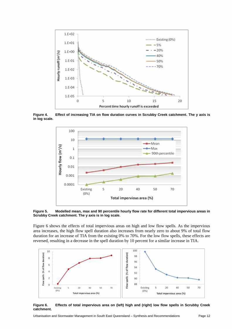
Figure 5 shows effects of different TIA on mean, maximum and top 90 percentile hourly flows. As the
impervious area increases, the top 90 percentile flow also increases. For Scrubby Creek, the fact that
the top 90 percentile flow is less than mean indicates that the mean flow is dominated by a few very
large flows in an otherwise low flow regime.
Urbanisation and Stormwater Management in South East Queensland – Synthesis and Recommendations Page 12
Figure 4. Effect of increasing TIA on flow duration curves in Scrubby Creek catchment. The y axis is in log scale.
Figure 5. Modelled mean, max and 90 percentile hourly flow rate for different total impervious areas in Scrubby Creek catchment. The y axis is in log scale.
Figure 6 shows the effects of total impervious areas on high and low flow spells. As the impervious
area increases, the high flow spell duration also increases from nearly zero to about 9% of total flow
duration for an increase of TIA from the existing 0% to 70%. For the low flow spells, these effects are
reversed, resulting in a decrease in the spell duration by 10 percent for a similar increase in TIA.
Figure 6. Effects of total impervious area on (left) high and (right) low flow spells in Scrubby Creek catchment.
Urbanisation and Stormwater Management in South East Queensland – Synthesis and Recommendations Page 13
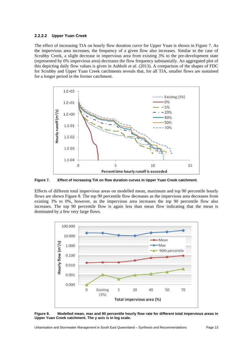
2.2.2.2 Upper Yuan Creek
The effect of increasing TIA on hourly flow duration curve for Upper Yuan is shown in Figure 7. As
the impervious area increases, the frequency of a given flow also increases. Similar to the case of
Scrubby Creek, a slight decrease in impervious area from existing 3% to the pre-development state
(represented by 0% impervious area) decreases the flow frequency substantially. An aggregated plot of
this depicting daily flow values is given in Ashbolt et al. (2013). A comparison of the shapes of FDC
for Scrubby and Upper Yuan Creek catchments reveals that, for all TIA, smaller flows are sustained
for a longer period in the former catchment.
Figure 7. Effect of increasing TIA on flow duration curves in Upper Yuan Creek catchment.
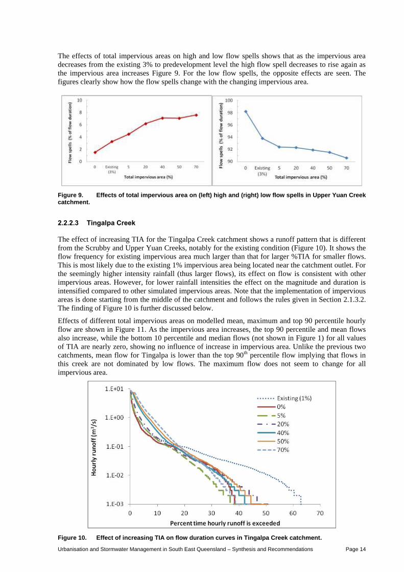
Effects of different total impervious areas on modelled mean, maximum and top 90 percentile hourly
flows are shown Figure 8. The top 90 percentile flow decreases as the impervious area decreases from
existing 3% to 0%, however, as the impervious area increases the top 90 percentile flow also
increases. The top 90 percentile flow is again less than mean flow indicating that the mean is
dominated by a few very large flows.
Figure 8. Modelled mean, max and 90 percentile hourly flow rate for different total impervious areas in Upper Yuan Creek catchment. The y axis is in log scale.
Urbanisation and Stormwater Management in South East Queensland – Synthesis and Recommendations Page 14
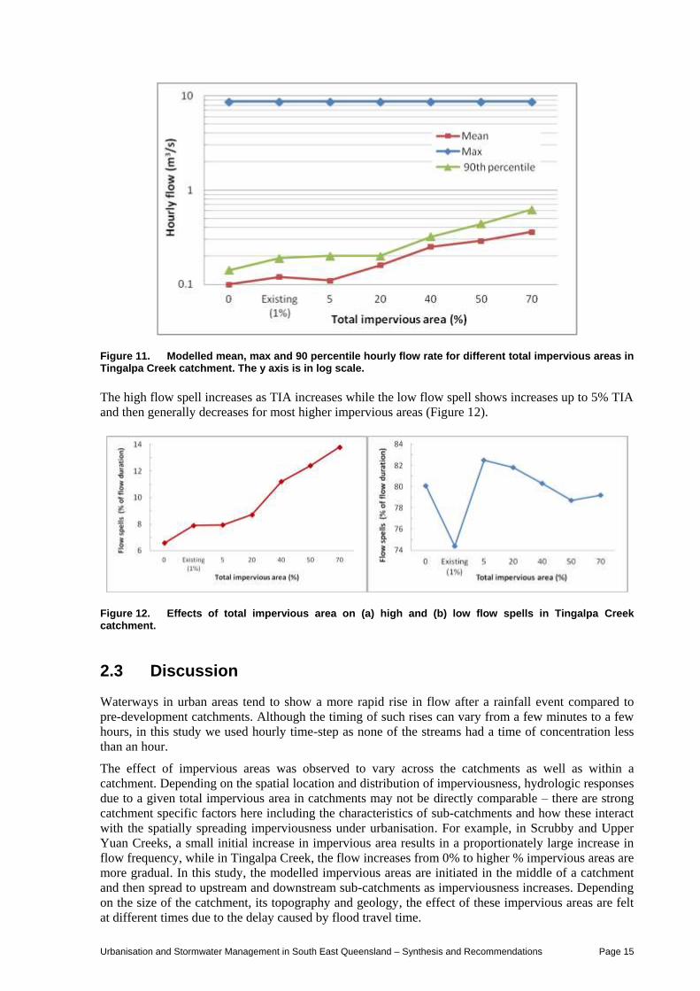
The effects of total impervious areas on high and low flow spells shows that as the impervious area
decreases from the existing 3% to predevelopment level the high flow spell decreases to rise again as
the impervious area increases Figure 9. For the low flow spells, the opposite effects are seen. The
figures clearly show how the flow spells change with the changing impervious area.
Figure 9. Effects of total impervious area on (left) high and (right) low flow spells in Upper Yuan Creek catchment.
2.2.2.3 Tingalpa Creek
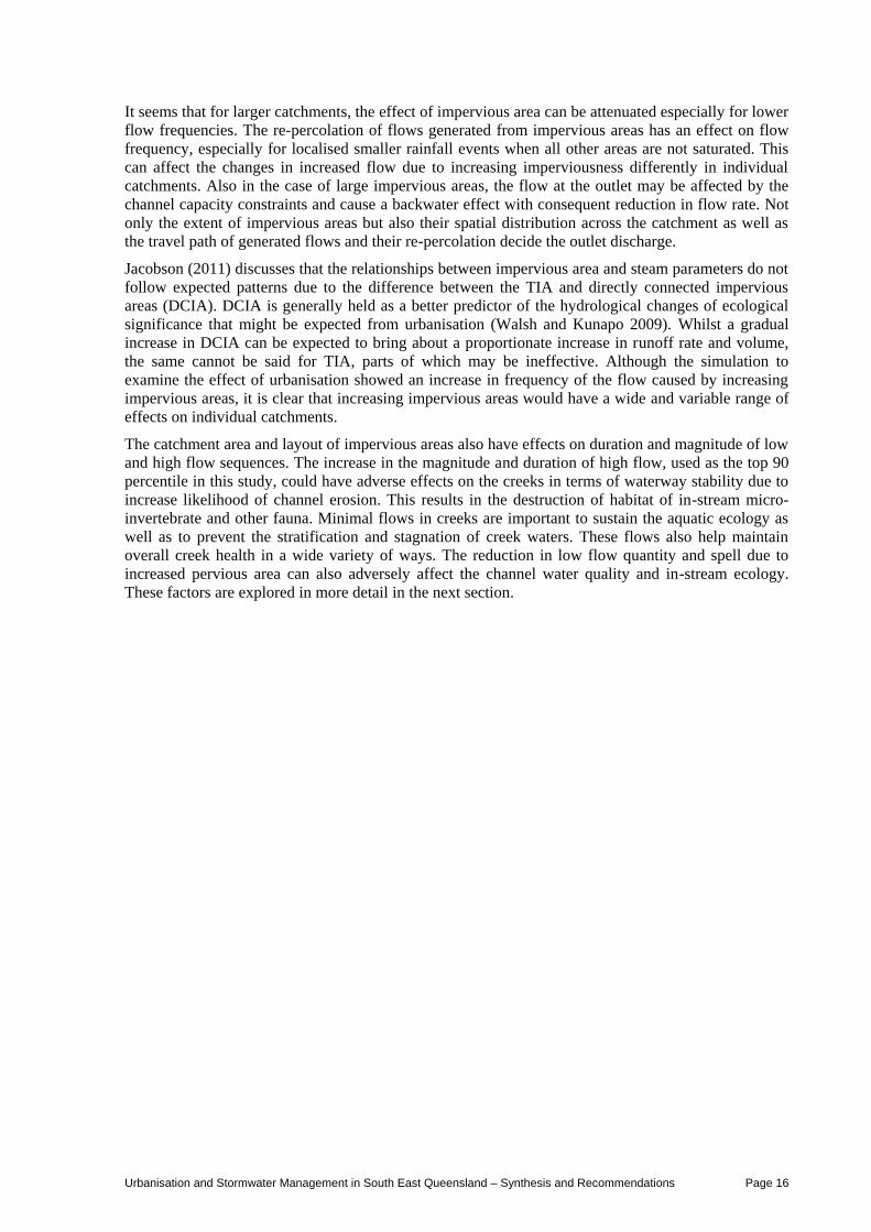
The effect of increasing TIA for the Tingalpa Creek catchment shows a runoff pattern that is different
from the Scrubby and Upper Yuan Creeks, notably for the existing condition (Figure 10). It shows the
flow frequency for existing impervious area much larger than that for larger %TIA for smaller flows.
This is most likely due to the existing 1% impervious area being located near the catchment outlet. For
the seemingly higher intensity rainfall (thus larger flows), its effect on flow is consistent with other
impervious areas. However, for lower rainfall intensities the effect on the magnitude and duration is
intensified compared to other simulated impervious areas. Note that the implementation of impervious
areas is done starting from the middle of the catchment and follows the rules given in Section 2.1.3.2.
The finding of Figure 10 is further discussed below.
Effects of different total impervious areas on modelled mean, maximum and top 90 percentile hourly
flow are shown in Figure 11. As the impervious area increases, the top 90 percentile and mean flows
also increase, while the bottom 10 percentile and median flows (not shown in Figure 1) for all values
of TIA are nearly zero, showing no influence of increase in impervious area. Unlike the previous two
catchments, mean flow for Tingalpa is lower than the top 90th percentile flow implying that flows in
this creek are not dominated by low flows. The maximum flow does not seem to change for all
impervious area.
Figure 10. Effect of increasing TIA on flow duration curves in Tingalpa Creek catchment.
Urbanisation and Stormwater Management in South East Queensland – Synthesis and Recommendations Page 15
Figure 11. Modelled mean, max and 90 percentile hourly flow rate for different total impervious areas in Tingalpa Creek catchment. The y axis is in log scale.
The high flow spell increases as TIA increases while the low flow spell shows increases up to 5% TIA
and then generally decreases for most higher impervious areas (Figure 12).
Figure 12. Effects of total impervious area on (a) high and (b) low flow spells in Tingalpa Creek catchment.
2.3 Discussion
Waterways in urban areas tend to show a more rapid rise in flow after a rainfall event compared to
pre-development catchments. Although the timing of such rises can vary from a few minutes to a few
hours, in this study we used hourly time-step as none of the streams had a time of concentration less
than an hour.
The effect of impervious areas was observed to vary across the catchments as well as within a
catchment. Depending on the spatial location and distribution of imperviousness, hydrologic responses
due to a given total impervious area in catchments may not be directly comparable – there are strong
catchment specific factors here including the characteristics of sub-catchments and how these interact
with the spatially spreading imperviousness under urbanisation. For example, in Scrubby and Upper
Yuan Creeks, a small initial increase in impervious area results in a proportionately large increase in
flow frequency, while in Tingalpa Creek, the flow increases from 0% to higher % impervious areas are
more gradual. In this study, the modelled impervious areas are initiated in the middle of a catchment
and then spread to upstream and downstream sub-catchments as imperviousness increases. Depending
on the size of the catchment, its topography and geology, the effect of these impervious areas are felt
at different times due to the delay caused by flood travel time.
Urbanisation and Stormwater Management in South East Queensland – Synthesis and Recommendations Page 16
It seems that for larger catchments, the effect of impervious area can be attenuated especially for lower
flow frequencies. The re-percolation of flows generated from impervious areas has an effect on flow
frequency, especially for localised smaller rainfall events when all other areas are not saturated. This
can affect the changes in increased flow due to increasing imperviousness differently in individual
catchments. Also in the case of large impervious areas, the flow at the outlet may be affected by the
channel capacity constraints and cause a backwater effect with consequent reduction in flow rate. Not
only the extent of impervious areas but also their spatial distribution across the catchment as well as
the travel path of generated flows and their re-percolation decide the outlet discharge.
Jacobson (2011) discusses that the relationships between impervious area and steam parameters do not
follow expected patterns due to the difference between the TIA and directly connected impervious
areas (DCIA). DCIA is generally held as a better predictor of the hydrological changes of ecological
significance that might be expected from urbanisation (Walsh and Kunapo 2009). Whilst a gradual
increase in DCIA can be expected to bring about a proportionate increase in runoff rate and volume,
the same cannot be said for TIA, parts of which may be ineffective. Although the simulation to
examine the effect of urbanisation showed an increase in frequency of the flow caused by increasing
impervious areas, it is clear that increasing impervious areas would have a wide and variable range of
effects on individual catchments.
The catchment area and layout of impervious areas also have effects on duration and magnitude of low
and high flow sequences. The increase in the magnitude and duration of high flow, used as the top 90
percentile in this study, could have adverse effects on the creeks in terms of waterway stability due to
increase likelihood of channel erosion. This results in the destruction of habitat of in-stream micro-
invertebrate and other fauna. Minimal flows in creeks are important to sustain the aquatic ecology as
well as to prevent the stratification and stagnation of creek waters. These flows also help maintain
overall creek health in a wide variety of ways. The reduction in low flow quantity and spell due to
increased pervious area can also adversely affect the channel water quality and in-stream ecology.
These factors are explored in more detail in the next section.
Urbanisation and Stormwater Management in South East Queensland – Synthesis and Recommendations Page 17
3. UNDERSTANDING HOW URBANISATION IMPACTS STREAM ECOLOGY IN SOUTH EAST QUEENSLAND
The report by Sheldon et al. (2012a) provides a full account of the urban stream ecology research
conducted during the project. The aim of this section is to summarise the key results so that the reader
is presented with a synthesis of the project hydrology and ecology findings in a single document.
The ecological consequences of changed catchment hydrology under conditions of urbanisation
(higher levels of impervious area) were investigated using two methods – large spatial scale, long term
analysis of the relationships between %TIA, directly connected IA and urban land cover and indicators
of ecosystem health from the SEQ Ecosystem Health Monitoring Program (EHMP -
http://healthywaterways.org/ehmphome.aspx), and field based ecological sampling of macroinvertebrates
from three case study sites along a disturbance gradient of %TIA. Directly connected impervious area
is that impervious area which has a direct hydraulic or overland flow connection to waterways (see
Walsh and Kunapo 2009, and Walsh et al. 2005 for details).
The aim of each method was twofold – (i) to characterise the kinds of ecological changes associated
with increasing urbanisation, and (ii) to determine the mechanisms of that change. Underlying the
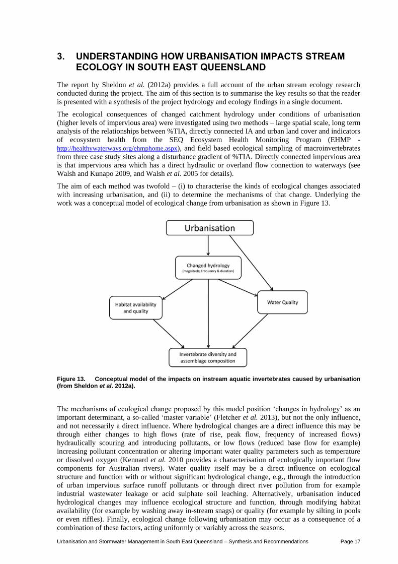
work was a conceptual model of ecological change from urbanisation as shown in Figure 13.
Figure 13. Conceptual model of the impacts on instream aquatic invertebrates caused by urbanisation (from Sheldon et al. 2012a).
The mechanisms of ecological change proposed by this model position ‘changes in hydrology’ as an
important determinant, a so-called ‘master variable’ (Fletcher et al. 2013), but not the only influence,
and not necessarily a direct influence. Where hydrological changes are a direct influence this may be
through either changes to high flows (rate of rise, peak flow, frequency of increased flows)
hydraulically scouring and introducing pollutants, or low flows (reduced base flow for example)
increasing pollutant concentration or altering important water quality parameters such as temperature
or dissolved oxygen (Kennard et al. 2010 provides a characterisation of ecologically important flow
components for Australian rivers). Water quality itself may be a direct influence on ecological
structure and function with or without significant hydrological change, e.g., through the introduction
of urban impervious surface runoff pollutants or through direct river pollution from for example
industrial wastewater leakage or acid sulphate soil leaching. Alternatively, urbanisation induced
hydrological changes may influence ecological structure and function, through modifying habitat
availability (for example by washing away in-stream snags) or quality (for example by silting in pools
or even riffles). Finally, ecological change following urbanisation may occur as a consequence of a
combination of these factors, acting uniformly or variably across the seasons.
Urbanisation and Stormwater Management in South East Queensland – Synthesis and Recommendations Page 18
Unpicking the kinds and causes of waterway ecological change which are associated with urbanisation
in SEQ is vital to being able to (i) determine the significance of the problem and (ii) provide
recommendations as to how they might be remedied. The aim of this section is to provide both that
characterisation and to characterise what we know about their causes. We will first examine the kinds
of changes which are associated with urbanisation at a large spatial scale and whether they are related
to TIA or to directly connected IA (DCIA), using the results from the TIA-EHMP analysis. Then we
will examine the results of the case study work to characterise the changes observed in terms of
macroinvertebrate assemblage composition between urban and non-urban (pre-development) sites, and
how these are related to hydrology and water quality over the course of a year (i.e. seasonally).
3.1 Impacts of Impervious Area on Ecosystem Health
3.1.1 Introduction and Aims
SEQ is fortunate to have in place a large scale, long running Ecosystem Health Monitoring Program
(EHMP). Details of the EHMP can be found elsewhere (http://healthywaterways.org/ehmphome.aspx
and links to reports from within that site), but essentially the program has served for over 10 years to
collect data on important indicators of river and estuarine aquatic ecosystem health for every
catchment in SEQ. These indicators include, for freshwater systems, water quality variables including
pH, dissolved oxygen, temperature; macroinvertebrate ecological variables including PET richness
(PET are sensitive species Plecoptera (stoneflies), Ephemeroptera (mayflies) and Trichoptera
(caddisflies)) and average SIGNAL score; and fish ecological variables including proportion of alien
fish species and the proportion of native species expected. A full list of variables and methods for
gathering the data can be found at
http://healthywaterways.org/EcosystemHealthMonitoringProgram/ProgramComponents/FreshwaterMonitoring/MethodsandIndicators.aspx.
Indicator values are calculated based on the data gathered and then summarised further using a single
EHMP score, which provides a synthesised view of the ecosystem health of a particular catchment or
sub-catchment or estuarine area, and, if examined over time, how that health has varied. Knowledge of
how the individual indicators and overall score have varied over time provides a means of identifying
where and what kinds of policy and management interventions are required to improve or avoid
degradation in ecosystem health, and a way of monitoring and adaptively managing on-going
management actions to improve their effectiveness.
EHMP data is gathered for over 130 different sub-catchments across SEQ, most of which do not
contain significant urbanisation, but some do. Sheldon et al. (2012b) and Petersen et al. (2011) had
previously analysed the impact of different land uses on EHMP score and indicator values, but had
only considered urban as a lumped land use, showing that it has a significant impact ecologically.
Impervious area had not been characterised and analysed as an influencing variable, so an analysis was
undertaken to determine if impervious area, either as lumped TIA, or inversely weighted to provide a
proxy for directly connected impervious area (DCIA – see Walsh and Kunapo 2009 on using inversely
weighted TIA as a proxy) is a significant influence on river aquatic ecosystem health. Demonstrating
that either TIA or DCIA is a significant influence would support changes in hydrology occurring from
increased urban runoff as being an important mechanism of ecological impact from urbanisation.
3.1.2 Methods
The methods employed for the statistical analysis of the relationships between EHMP score,
indicators, urban land use and TIA are fully described in Sheldon et al. (2012b), Sheldon et al. (2012a)
and Peterson et al. (2011). TIA was analysed based on various methods of spatially aggregating the
rasters of impervious area within catchments to mimic potential variations in hydraulic connection
with the stream and catchment outlet. Six spatial aggregation metrics were used - (i) Lumped;
(ii) iFLO; (iii) iFLS; (iv) HA-iFLO; (v) HA-iFLS; and (vi) iEuc. Figure 14 from Peterson et al. (2011)
illustrates the metrics and how they differentially weight cells according to their location. By summing
the weighted TIA values for all cells in the landscape, under each weighting, a total TIA and
consequently a weighted % TIA or TIA metric, was obtained for use in statistical analysis with the
EHMP score and component indicators.
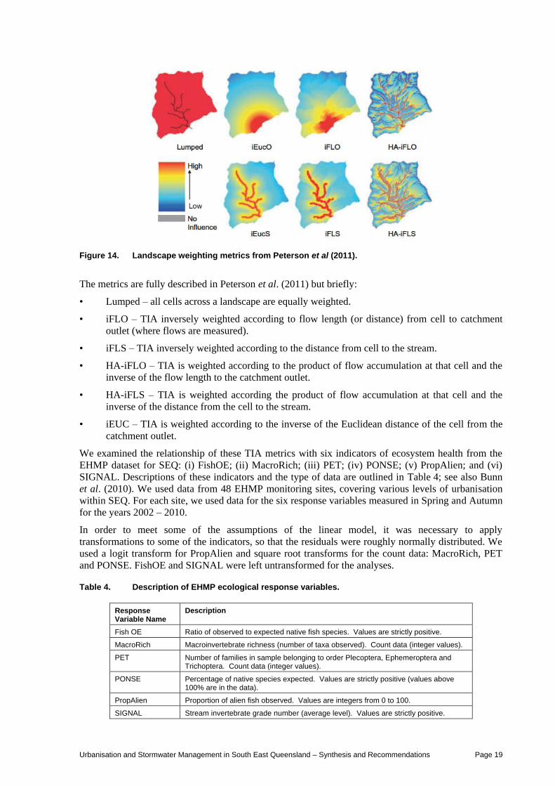
Urbanisation and Stormwater Management in South East Queensland – Synthesis and Recommendations Page 19
Figure 14. Landscape weighting metrics from Peterson et al (2011).
The metrics are fully described in Peterson et al. (2011) but briefly:
• Lumped – all cells across a landscape are equally weighted.
• iFLO – TIA inversely weighted according to flow length (or distance) from cell to catchment
outlet (where flows are measured).
• iFLS – TIA inversely weighted according to the distance from cell to the stream.
• HA-iFLO – TIA is weighted according to the product of flow accumulation at that cell and the
inverse of the flow length to the catchment outlet.
• HA-iFLS – TIA is weighted according the product of flow accumulation at that cell and the
inverse of the distance from the cell to the stream.
• iEUC – TIA is weighted according to the inverse of the Euclidean distance of the cell from the
catchment outlet.
We examined the relationship of these TIA metrics with six indicators of ecosystem health from the
EHMP dataset for SEQ: (i) FishOE; (ii) MacroRich; (iii) PET; (iv) PONSE; (v) PropAlien; and (vi)
SIGNAL. Descriptions of these indicators and the type of data are outlined in Table 4; see also Bunn
et al. (2010). We used data from 48 EHMP monitoring sites, covering various levels of urbanisation
within SEQ. For each site, we used data for the six response variables measured in Spring and Autumn
for the years 2002 – 2010.
In order to meet some of the assumptions of the linear model, it was necessary to apply
transformations to some of the indicators, so that the residuals were roughly normally distributed. We
used a logit transform for PropAlien and square root transforms for the count data: MacroRich, PET
and PONSE. FishOE and SIGNAL were left untransformed for the analyses.
Table 4. Description of EHMP ecological response variables.
Response Variable Name
Description
Fish OE Ratio of observed to expected native fish species. Values are strictly positive.
MacroRich Macroinvertebrate richness (number of taxa observed). Count data (integer values).
PET Number of families in sample belonging to order Plecoptera, Ephemeroptera and Trichoptera. Count data (integer values).
PONSE Percentage of native species expected. Values are strictly positive (values above 100% are in the data).
PropAlien Proportion of alien fish observed. Values are integers from 0 to 100.
SIGNAL Stream invertebrate grade number (average level). Values are strictly positive.
Urbanisation and Stormwater Management in South East Queensland – Synthesis and Recommendations Page 20
A number of important environmental covariates were also collected for each of the EHMP sites.
These covariates included other land use metrics (see Sheldon et al. 2012b), physico-chemical
measurements, modelled stream flow data and seasonal information (see Sheldon et al. 2012b). By
incorporating some of these covariates into the statistical analyses, it was hoped that the linear model
error variance could be reduced, increasing the ability of the analysis to detect significant relationships
between the calculated TIA metrics and the ecological response variables.
3.1.3 Results
For the fish response metrics no land-use measure at the scales included had a strong inclusion
probability for modelled FishOE. Dense Forest (DF) close to the site (metric HA-iFLS DF) had the
highest inclusion probability for modelled PONSE, while the presence of very sparse forest (VSP) in
the riparian zone or close to the site influenced the proportion of alien species present. Of the TIA
metrics, TIA iEuc was the only metric of importance, with an inclusion probability of 0.4 for PONSE,
indicating a likely influence of DCIA (proxied by inverse Euclidean distance TIA) on fish ecology.
For the macroinvertebrate response metrics, measures of urbanisation were important for family
richness (MacroRich), with urbanisation anywhere in the catchment or in the riparian zone important.
The macroinvertebrate metric SIGNAL, which relies heavily on the presence of insect taxa, was
mostly influenced by dense forest at the site (DF iFLO), which intuitively makes sense as many of the
insect taxa have a terrestrial adult phase which requires riparian cover.
Overall, TIA metrics were included in the models approximately 38% of the time. TIA metrics were
also present as explanatory variables for modelling FishOE, with an overall inclusion of almost 7%,
which were again spread mostly between the iEuc and HA-iFLO metrics. Inclusion probabilities of
TIA metrics in the remaining models were very small.
Whilst the TIA metrics may not have featured heavily in the models, urban land use metrics featured
strongly in modeling MacroRich and PropAlien with member variables included in of 99% and 94%
of models respectively. For both response variables, lumped riparian, lumped watershed and iFLS
metrics were included most frequently, and these lumped measures of urbanisation may be reflective
of impervious connection which can occur anywhere in the catchment.
Regarding the water quality (physico-chemical) variables - for MacroRich, temperature range was
included in 47% of models. Minimum dissolved oxygen was included in approximately 35% of
models for PET and 95% of the models for SIGNAL. For PONSE, pH was included as a predictor in
52% of models. PropAlien had a number of useful predictor variables, with pH, temperature range and
minimum dissolved oxygen included in 21%, 20% and 33% of models respectively.
3.1.4 Conclusions
While %TIA was not a major driving predictor for any of the ecological response variables, the
importance of urbanisation and particularly the lumped measures of urbanisation suggest the influence
of connection of impervious areas on the health of streams, as measured by these macroinvertebrate
and fish indicators, may be significant. This insight is new and begs the question – why does the
aggregate measure of urbanisation show a negative impact ecologically on streams, whilst the
generally accepted hydraulically relevant measure (Fletcher et al. 2008), impervious area (IA),
weighted to both represent undifferentiated TIA as well as directly connected or hydraulically active
IA, not show any negative impact? There are a number of possible explanations which are
characterised below:
(1) ‘Impervious area not in the right place’ – the imperviousness in the urban catchments studied
could have been generally located either far away from streams or variably so from catchment
to catchment. Such variation could have masked the influence of TIA, which may still be
exerting the expected negative impact from changes to stream hydrology occurring from
changes to runoff.
Urbanisation and Stormwater Management in South East Queensland – Synthesis and Recommendations Page 21
(2) ‘Not enough TIA’ – the EHMP scheme was not explicitly set up to monitor the impact of
urbanisation and so the number and range of urban sites may not best suit the question being
asked. In addition, only a limited number of the urban sites could be analysed to characterise
TIA due to labour and cost constraints.
(3) ‘Urbanisation does the damage’ – perhaps in a sub-tropical climate such as in SEQ the on-going
impacts of changed hydrology from urban IA are relatively minor compared to the initial,
significant stream morphology, habitat and biotic impacts which occur during the process of
construction? Streams in SEQ often have naturally significantly high peak flows due to the high
intensity summer rainfall, and in larger catchments such as the Tingalpa studied in this project,
the frequency of high flows can be high. Such catchments vary qualitatively in their behaviour
from catchments in more temperate climates, where much of the research into the relationships
between urbanisation and stream hydrology has been undertaken. If high flows and high peak
flows are the norm, then perhaps the relative hydrologic impact of urbanisation is less
significant in SEQ than in, say, Melbourne.
So, how might one decide between these alternative explanations? First of all one might ask whether
there is a relationship between the total % of urban cover in the catchments examined and the value of
the hydrologically active and inverse stream flow metrics HA-iFLS and iFLS, which best characterise
directly connected or hydraulically active urban areas? Does urban cover and consequently IA tend to
occur near or far from streams and the catchment outlet? Figure 15 below shows the relationships
between lumped urban area (x-axis) and the four key metrics – iFLO, iFLS, HA-iFLO and HA-iFLS.
Figure 15. Relationships between total catchment urban area (% area, x-axis) and four urban area metrics (weighted % area, y-axis) across the 36 most urbanised EHMP catchments.
Figure 15 shows a variable but generally increasing trend towards more urban areas near streams
(iFLS), near the catchment outlets (iFLO) and near the hydrologically active area around streams (HA-
iFLS) and the catchment outlet (HA-iFLO) with increasing total urban area. The relationship between
total urban area and urban areas near the hydrological active area around the catchment outlet (HA-
iFLO) is variable and not clear. This suggests that generally, as urban area increases, more urban area
is found near locations where it is likely to play an active role in modifying hydrology, and
consequently that one would expect, if all urban area is equally impervious, that imperviousness is in
the right location to exert a hydrological impact. Of course not all urban area is equally impervious.
Figure 16 shows how TIA varies with increasing % coverage of urban area in a catchment – TIA does
not vary uniformly with urban area. Urban areas in some catchments are more impervious than in
others.
Urbanisation and Stormwater Management in South East Queensland – Synthesis and Recommendations Page 22
0
5000
10000
15000
20000
25000
30000
35000
40000
45000
50000
0 10 20 30 40 50 60 70 80 90 100
TIALumped
Figure 16. Relationships between total catchment urban area (% area, x-axis) and lumped (non-weighted) lumped TIA area (m2, y-axis) across the 9 most urbanised EHMP catchments.
Combining variability in the imperviousness of urban area between catchments with variability in the
location of urban area (and consequently imperviousness) across catchments could well be masking
the impact of IA, and in particular TIA, which will likely lead to a weaker relationship between
increasing total TIA and the key hydrologically relevant TIA metrics – iFLS, iFLO, HA-iFLS & HA-
iFLO.
The data in Figure 15 covers the 36 EHMP catchments which have greater than or equal to 10% total
urban area. The actual TIA analysis only included a smaller number, the 9 EHMP catchments with
greater than 50% total urban area, primarily because of the cost of the digital photographs for TIA
characterisation and the length of the characterisation process. To further understand the direct role of
TIA on stream health, over and above the general impact of urbanisation, at broad spatial scales we
need a more mechanistic way of calculating TIA in upstream catchments. This analysis included only
a portion of the total sites available as part of the EHMP dataset due to the laborious manner in which
TIA needs calculating. If all 130 EHMP sites could be used and TIA calculated, then a better
understanding of the role of impervious area on stream health would be obtained, remembering of
course that within urban areas it is not just impervious area that influences stream degradation, a better
predictor may be connected impervious area as TIA that is directly connected to streams via the
stormwater network may have a greater negative impact on stream health than unconnected areas.
Interestingly, one of the ways in which urbanisation appears to manifest impacts on
macroinvertebrates and fish is through changes to water quality, and particularly through reduced
dissolved oxygen owing to the higher organic load in runoff draining urban areas. In this analysis,
minimum dissolved oxygen was an important predictor for both PET richness and SIGNAL score.
Both these metrics rely heavily on the presence and abundance of sensitive insect taxa, mainly the
Plecoptera (stoneflies), Ephemeroptera (mayflies) and Trichoptera (caddisflies). So there is sufficient
evidence that urbanisation causes ecological impacts.
But are these impacts (i) an on-going consequence of the changes to hydrology following the building
of impervious area as part of urbanisation, or (ii) were the impacts primarily caused by the process of
construction – levelling ground, clearing vegetation, changing channel morphology – at the time of
construction or shortly afterwards? That is, are the stream systems still adjusting to a new dynamic
equilibrium in structural, hydrologic and ecological terms as under (i) or have they been in dynamic
equilibrium for some time and no longer significantly being impacted by changed hydrology as under
(ii)? Based on the evidence we have analysed here, we can say that TIA, even when weighted to proxy
the effect of directly connected impervious area, is unlikely to be exerting a significant impact
ecologically. This would suggest (ii); that the EHMP catchments are not continuing to degrade
ecologically in adjustment to hydrological changes from urbanisation, but rather they have already
adjusted.
Urbanisation and Stormwater Management in South East Queensland – Synthesis and Recommendations Page 23
However, as shown in Figure 15 and Figure 16 and explained above, we cannot be certain of this –
urban land use and in particular IA location and the extent of urban imperviousness is variable across
catchments in relation to hydraulic connectivity to streams, and this variability may be masking the
hydrological and consequently ecological impacts created. To clarify the situation, a fuller analysis of
urban land use and TIA across all EHMP catchments is required, and ideally, in addition, research to
better understand how hydrological changes occur during and shortly after construction processes. Are
there rapid changes, or are they more strung out temporally? What changes happen quickly and which
ones slowly? How do those hydrologic changes influence habitat, water quality and consequently
ecology? These are important questions for they suggest qualitatively different interventions –
construction phase control (e.g. sediment erosion control) or water sensitive urban design.
3.2 Focussed Temporal Analysis
3.2.1 Introduction and Aims
Three sites were chosen for a more focussed temporal investigation of hydrological, water quality and
macroinvertebrate changes throughout a 12 month period, from dry to wet conditions (winter through
summer). These sites were chosen based on (i) similarities in riparian cover - we were aiming to
reduce riparian cover as a driving variable in differences, and (ii) the fact that they all had hydrological
monitoring stations, collecting both daily flow data and water quality. The three sites included
Tingalpa Creek (Forested treatment – pre-development), Blunder Creek tributary at Carolina Parade
(‘Water-Sensitive Urban Design’ treatment) and Stable Swamp Creek (Urban treatment).
As described in section 2, Tingalpa Creek is an upland creek in the Redlands City Council area, the
upstream portion of the creek is completely forested, the channel comprises bedrock riffles, runs and
pools with complex microhabitats of snags (fallen timber), tree roots and macrophytes. Stable Swamp
Creek and the tributary to Blunder Creek are both in the Oxley-Blunder Creek sub-catchment that
drains into the Brisbane River. The upstream reaches of Stable Swamp Creek are highly urbanised, the
channel is degraded and greatly incised, pools have deep silt with poor habitat quality, mostly
dominated by thick introduced macrophytes, the one riffle below the road culvert was likely placed in
the channel during early attempts at channel restoration. The WSUD site on the tributary to Blunder
Creek is downstream of Forest Lake, a large stormwater retention basin; the channel is deeply incised
and degraded with mostly poor habitat quality. The presence of good riparian vegetation on both
banks, however, has allowed some riffle development along the channel.
Based on the conceptual model in Figure 13, we predicted that: (i) diversity in the urban site (Stable
Swamp Creek) would be lower than in either Tingalpa Creek or the tributary to Blunder Creek and
dominated by more tolerant taxa (worms, snails etc), in contrast Tingalpa Creek would have the
highest diversity and be dominated by PET taxa; (ii) all sites should be more similar in the winter
when flows are similar and should diverge more in summer when the urban site is subject to a greater
frequency of high flows; and (iii) the abundance of specific fauna (eg. PETs) on the same microhabitat
across all three sites should be different in the summer when the urban sites are subjected to a higher
frequency of high flow.
To test these predictions, an analysis of between site and within site differences over the year of
sampling was undertaken examining differences in (i) hydrology, (ii) water quality and (iii)
macroinvertebrate assemblage composition and diversity. Macroinvertebrates were selected as a
sensitive and useful indicator of ecosystem health. This section will provide reporting into the key
results in each area. For full results and a description of the methods the reader is referred to Sheldon
et al. (2012a).
3.2.2 Hydrological Differences
To complement the longer term modelling analysis documented in section 2, analysis of the gauged
flow data at each site was undertaken for the period from 2009 until the end of 2012. Full details of the
gauging method can be found in Chowdhury et al. (2012).
Urbanisation and Stormwater Management in South East Queensland – Synthesis and Recommendations Page 24
When individual flow metrics were explored separately, there was no significant difference in the
number of rises in each month (F11,60=1.507, p>0.05) but a significant difference between sites
(F2,60=16.283, p<0.001) with no significant interaction (F21,60=1.14, p>0.05). The forested Tingalpa
Creek had significantly fewer rises than both the urbanised Stable Swamp Creek and the tributary to
Blunder Creek (Figure 17). For mean daily flow, there was no significant interaction between site and
month (F21,60=0.809, p>0.05), but a significant difference between months (F11,60=2.15, p=0.03) and
between sites (F2,60=5.828, p<0.01). The mean daily flow was significantly higher in Stable Swamp
Creek than either Tingalpa Creek or the tributary to Blunder Creek (Figure 18).
For the metrics that describe the rise and fall of flow events, there were significant differences
between months (F11,60=2.185, p<0.05) and sites (F2,60=3.791, P<0.05) but no significant interaction
(F21,60=0.537, p>0.05), with Tingalpa Creek having significantly smaller magnitudes of flow pulse
rises than Stable Swamp Creek (Figure 19). Across all sites, the magnitude of the rises was smaller
during the drier months (May – September) compared with the seasonally wet months (December –
March). A similar pattern was found for the mean magnitude of the falling limb of a flow pulse with a
significant difference between sites (F2,60=4.161, p<0.05) and between months (F11,60=2.597, p<0.01),
but no significant interaction between site and month (F21,60=0.690, p>0.05). Again, the difference was
between Tingalpa Creek and Stable Swamp Creek, with Tingalpa having the reduced magnitude of fall
(Figure 20). In both cases, the magnitudes of rise and falls are following that expected of urban
streams, with the highly urbanised Stable Swamp Creek having significantly greater magnitudes of
rise and fall than the forested Tingalpa Creek.
For minimum flow (Min), there was a significant difference between sites (F2,60=65.966, p<0.001) but
not between months (F11,60=0.289, p>0.05), with no interaction (F21,60=0.726, p>0.05); with Stable
Swamp Creek having significantly higher minimum flows then either Tingalpa Creek or the Blunder
Creek tributary (Figure 21). The same pattern was observed for the 10th percentile of flows (P10).
Interestingly, it is the higher base flows in Stable Swamp Creek during the drier winter months that are
dominant.
Figure 17. Mean number of flow rises (±SE) for months by site.
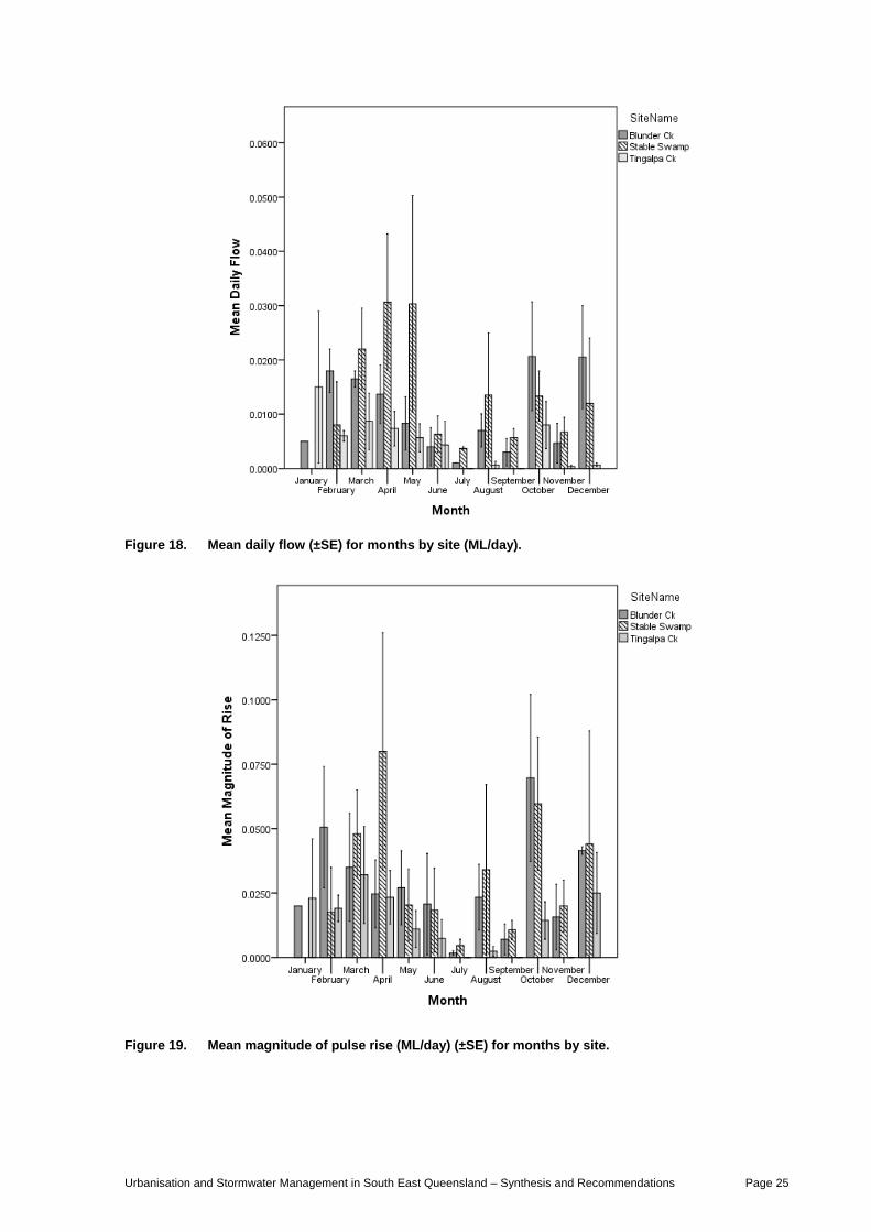
Urbanisation and Stormwater Management in South East Queensland – Synthesis and Recommendations Page 25
Figure 18. Mean daily flow (±SE) for months by site (ML/day).
Figure 19. Mean magnitude of pulse rise (ML/day) (±SE) for months by site.
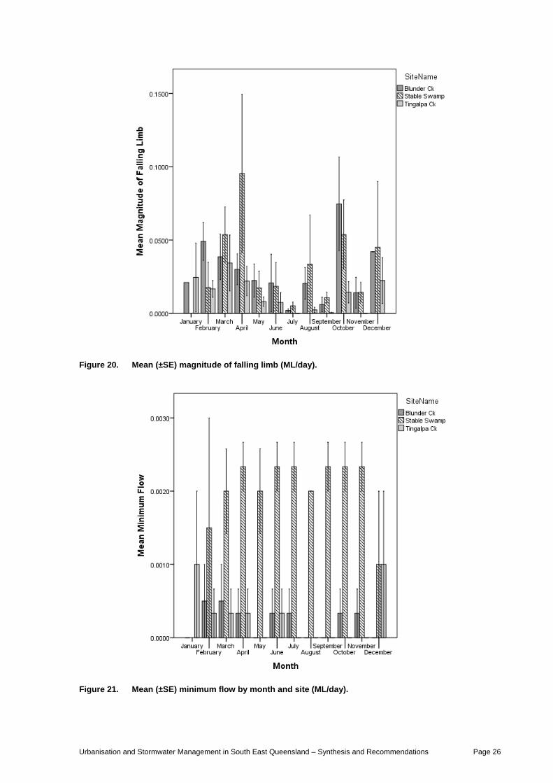
Urbanisation and Stormwater Management in South East Queensland – Synthesis and Recommendations Page 26
Figure 20. Mean (±SE) magnitude of falling limb (ML/day).
Figure 21. Mean (±SE) minimum flow by month and site (ML/day).
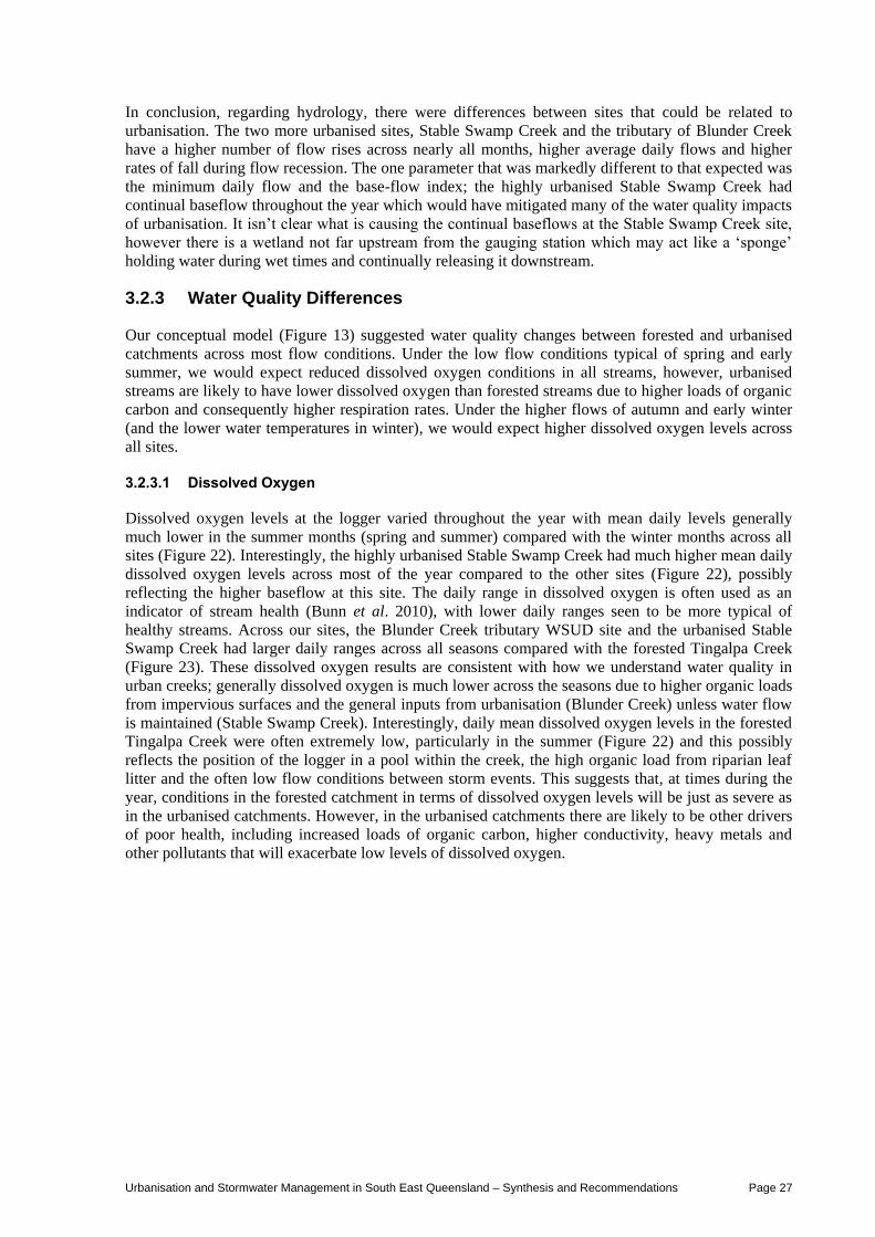
Urbanisation and Stormwater Management in South East Queensland – Synthesis and Recommendations Page 27
In conclusion, regarding hydrology, there were differences between sites that could be related to
urbanisation. The two more urbanised sites, Stable Swamp Creek and the tributary of Blunder Creek
have a higher number of flow rises across nearly all months, higher average daily flows and higher
rates of fall during flow recession. The one parameter that was markedly different to that expected was
the minimum daily flow and the base-flow index; the highly urbanised Stable Swamp Creek had
continual baseflow throughout the year which would have mitigated many of the water quality impacts
of urbanisation. It isn’t clear what is causing the continual baseflows at the Stable Swamp Creek site,
however there is a wetland not far upstream from the gauging station which may act like a ‘sponge’
holding water during wet times and continually releasing it downstream.
3.2.3 Water Quality Differences
Our conceptual model (Figure 13) suggested water quality changes between forested and urbanised
catchments across most flow conditions. Under the low flow conditions typical of spring and early
summer, we would expect reduced dissolved oxygen conditions in all streams, however, urbanised
streams are likely to have lower dissolved oxygen than forested streams due to higher loads of organic
carbon and consequently higher respiration rates. Under the higher flows of autumn and early winter
(and the lower water temperatures in winter), we would expect higher dissolved oxygen levels across
all sites.
3.2.3.1 Dissolved Oxygen
Dissolved oxygen levels at the logger varied throughout the year with mean daily levels generally
much lower in the summer months (spring and summer) compared with the winter months across all
sites (Figure 22). Interestingly, the highly urbanised Stable Swamp Creek had much higher mean daily
dissolved oxygen levels across most of the year compared to the other sites (Figure 22), possibly
reflecting the higher baseflow at this site. The daily range in dissolved oxygen is often used as an
indicator of stream health (Bunn et al. 2010), with lower daily ranges seen to be more typical of
healthy streams. Across our sites, the Blunder Creek tributary WSUD site and the urbanised Stable
Swamp Creek had larger daily ranges across all seasons compared with the forested Tingalpa Creek
(Figure 23). These dissolved oxygen results are consistent with how we understand water quality in
urban creeks; generally dissolved oxygen is much lower across the seasons due to higher organic loads
from impervious surfaces and the general inputs from urbanisation (Blunder Creek) unless water flow
is maintained (Stable Swamp Creek). Interestingly, daily mean dissolved oxygen levels in the forested
Tingalpa Creek were often extremely low, particularly in the summer (Figure 22) and this possibly
reflects the position of the logger in a pool within the creek, the high organic load from riparian leaf
litter and the often low flow conditions between storm events. This suggests that, at times during the
year, conditions in the forested catchment in terms of dissolved oxygen levels will be just as severe as
in the urbanised catchments. However, in the urbanised catchments there are likely to be other drivers
of poor health, including increased loads of organic carbon, higher conductivity, heavy metals and
other pollutants that will exacerbate low levels of dissolved oxygen.
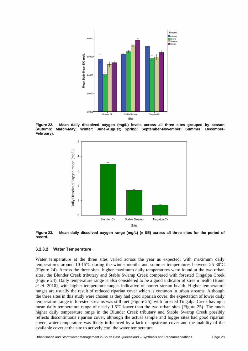
Urbanisation and Stormwater Management in South East Queensland – Synthesis and Recommendations Page 28
Figure 22. Mean daily dissolved oxygen (mg/L) levels across all three sites grouped by season (Autumn: March-May; Winter: June-August; Spring: September-November; Summer: December-February).
Site
Blunder Ck Stable Swamp Tingalpa Ck
Da
ily D
isso
lve
d O
xyge
n r
an
ge
(m
g/L
)
0
1
2
3
4
5
Figure 23. Mean daily dissolved oxygen range (mg/L) (± SE) across all three sites for the period of record.
3.2.3.2 Water Temperature
Water temperature at the three sites varied across the year as expected, with maximum daily
temperatures around 10-15oC during the winter months and summer temperatures between 25-30oC
(Figure 24). Across the three sites, higher maximum daily temperatures were found at the two urban
sites, the Blunder Creek tributary and Stable Swamp Creek compared with forested Tingalpa Creek
(Figure 24). Daily temperature range is also considered to be a good indicator of stream health (Bunn
et al. 2010), with higher temperature ranges indicative of poorer stream health. Higher temperature
ranges are usually the result of reduced riparian cover which is common in urban streams. Although
the three sites in this study were chosen as they had good riparian cover, the expectation of lower daily
temperature range in forested streams was still met (Figure 25), with forested Tingalpa Creek having a
mean daily temperature range of nearly 1.5oC lower than the two urban sites (Figure 25). The much
higher daily temperature range in the Blunder Creek tributary and Stable Swamp Creek possibly
reflects discontinuous riparian cover, although the actual sample and logger sites had good riparian
cover, water temperature was likely influenced by a lack of upstream cover and the inability of the
available cover at the site to actively cool the water temperature.
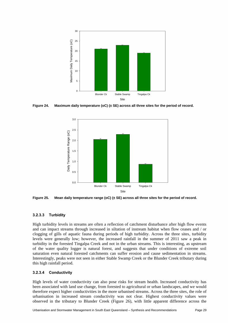
Urbanisation and Stormwater Management in South East Queensland – Synthesis and Recommendations Page 29
Site
Blunder Ck Stable Swamp Tingalpa Ck
Ma
xim
um
Da
ily T
em
pe
ratu
re (
oC
)
0
5
10
15
20
25
30
Figure 24. Maximum daily temperature (oC) (± SE) across all three sites for the period of record.
Site
Blunder Ck Stable Swamp Tingalpa Ck
Da
ily T
em
pe
ratu
re R
an
ge
(o
C)
0.0
0.5
1.0
1.5
2.0
2.5
3.0
Figure 25. Mean daily temperature range (oC) (± SE) across all three sites for the period of record.
3.2.3.3 Turbidity
High turbidity levels in streams are often a reflection of catchment disturbance after high flow events
and can impact streams through increased in siltation of instream habitat when flow ceases and / or
clogging of gills of aquatic fauna during periods of high turbidity. Across the three sites, turbidity
levels were generally low; however, the increased rainfall in the summer of 2011 saw a peak in
turbidity in the forested Tingalpa Creek and not in the urban streams. This is interesting, as upstream
of the water quality logger is natural forest, and suggests that under conditions of extreme soil
saturation even natural forested catchments can suffer erosion and cause sedimentation in streams.
Interestingly, peaks were not seen in either Stable Swamp Creek or the Blunder Creek tributary during
this high rainfall period.
3.2.3.4 Conductivity
High levels of water conductivity can also pose risks for stream health. Increased conductivity has
been associated with land use change, from forested to agricultural or urban landscapes, and we would
therefore expect higher conductivities in the more urbanised streams. Across the three sites, the role of
urbanisation in increased stream conductivity was not clear. Highest conductivity values were
observed in the tributary to Blunder Creek (Figure 26), with little apparent difference across the
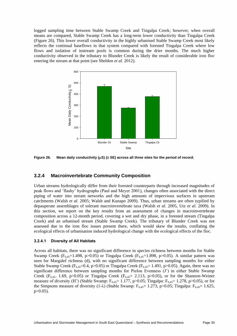
Urbanisation and Stormwater Management in South East Queensland – Synthesis and Recommendations Page 30
logged sampling time between Stable Swamp Creek and Tingalpa Creek; however, when overall
means are compared, Stable Swamp Creek has a long-term lower conductivity than Tingalpa Creek
(Figure 26). This lower overall conductivity in the highly urbanised Stable Swamp Creek most likely
reflects the continual baseflows in that system compared with forested Tingalpa Creek where low
flows and isolation of instream pools is common during the drier months. The much higher
conductivity observed in the tributary to Blunder Creek is likely the result of considerable iron floc
entering the stream at that point (see Sheldon et al. 2012).
Site
Blunder Ck Stable Swamp Tingalpa Ck
Me
an
Da
ily C
on
du
ctivity (
S)
0
100
200
300
400
500
600
Figure 26. Mean daily conductivity (S) (± SE) across all three sites for the period of record.
3.2.4 Macroinvertebrate Community Composition
Urban streams hydrologically differ from their forested counterparts through increased magnitudes of
peak flows and ‘flashy’ hydrographs (Paul and Meyer 2001), changes often associated with the direct
piping of water into stream networks and the high amounts of impervious surfaces in upstream
catchments (Walsh et al. 2005; Walsh and Kunapo 2009). Thus, urban streams are often typified by
depauperate assemblages of tolerant macroinvertebrate taxa (Walsh et al. 2005, Utz et al. 2009). In
this section, we report on the key results from an assessment of changes in macroinvertebrate
composition across a 12-month period, covering a wet and dry phase, in a forested stream (Tingalpa
Creek) and an urbanised stream (Stable Swamp Creek). The tributary of Blunder Creek was not
assessed due to the iron floc issues present there, which would skew the results, conflating the
ecological effects of urbanisation induced hydrological change with the ecological effects of the floc.
3.2.4.1 Diversity of All Habitats
Across all habitats, there was no significant difference in species richness between months for Stable
Swamp Creek (F6,45=1.498, p>0.05) or Tingalpa Creek (F6,45=1.898, p>0.05). A similar pattern was
seen for Margalef richness (d), with no significant difference between sampling months for either
Stable Swamp Creek (F6,45=0.4, p>0.05) or Tingalpa Creek (F6,45= 1.491, p>0.05). Again, there was no
significant difference between sampling months for Pielou Evenness (J’) in either Stable Swamp
Creek (F6,45= 1.69, p>0.05) or Tingalpa Creek (F6,45= 2.113, p>0.05), or for the Shannon-Weiner
measure of diversity (H’) (Stable Swamp: F6,45= 1.177, p>0.05; Tingalpa: F6,45= 1.278, p>0.05), or for
the Simpsons measure of diversity (1-λ) (Stable Swamp: F6,45= 1.273, p>0.05; Tingalpa: F6,45= 1.625,
p>0.05).
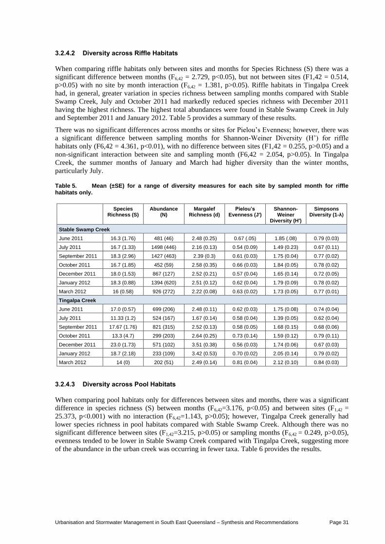
Urbanisation and Stormwater Management in South East Queensland – Synthesis and Recommendations Page 31
3.2.4.2 Diversity across Riffle Habitats
When comparing riffle habitats only between sites and months for Species Richness (S) there was a
significant difference between months (F6,42 = 2.729, p<0.05), but not between sites (F1,42 = 0.514,
p>0.05) with no site by month interaction (F6,42 = 1.381, p>0.05). Riffle habitats in Tingalpa Creek
had, in general, greater variation in species richness between sampling months compared with Stable
Swamp Creek, July and October 2011 had markedly reduced species richness with December 2011
having the highest richness. The highest total abundances were found in Stable Swamp Creek in July
and September 2011 and January 2012. Table 5 provides a summary of these results.
There was no significant differences across months or sites for Pielou’s Evenness; however, there was
a significant difference between sampling months for Shannon-Weiner Diversity (H’) for riffle
habitats only (F6,42 = 4.361, p<0.01), with no difference between sites (F1,42 = 0.255, p>0.05) and a
non-significant interaction between site and sampling month (F6,42 = 2.054, p>0.05). In Tingalpa
Creek, the summer months of January and March had higher diversity than the winter months,
particularly July.
Table 5. Mean (±SE) for a range of diversity measures for each site by sampled month for riffle habitats only.
Species Richness (S)
Abundance (N)
Margalef Richness (d)
Pielou’s Evenness (J')
Shannon-Weiner
Diversity (H')
Simpsons Diversity (1-λ)
Stable Swamp Creek
June 2011 16.3 (1.76) 481 (46) 2.48 (0.25) 0.67 (.05) 1.85 (.08) 0.79 (0.03)
July 2011 16.7 (1.33) 1498 (446) 2.16 (0.13) 0.54 (0.09) 1.49 (0.23) 0.67 (0.11)
September 2011 18.3 (2.96) 1427 (463) 2.39 (0.3) 0.61 (0.03) 1.75 (0.04) 0.77 (0.02)
October 2011 16.7 (1.85) 452 (59) 2.58 (0.35) 0.66 (0.03) 1.84 (0.05) 0.78 (0.02)
December 2011 18.0 (1.53) 867 (127) 2.52 (0.21) 0.57 (0.04) 1.65 (0.14) 0.72 (0.05)
January 2012 18.3 (0.88) 1394 (620) 2.51 (0.12) 0.62 (0.04) 1.79 (0.09) 0.78 (0.02)
March 2012 16 (0.58) 926 (272) 2.22 (0.08) 0.63 (0.02) 1.73 (0.05) 0.77 (0.01)
Tingalpa Creek
June 2011 17.0 (0.57) 699 (206) 2.48 (0.11) 0.62 (0.03) 1.75 (0.08) 0.74 (0.04)
July 2011 11.33 (1.2) 524 (167) 1.67 (0.14) 0.58 (0.04) 1.39 (0.05) 0.62 (0.04)
September 2011 17.67 (1.76) 821 (315) 2.52 (0.13) 0.58 (0.05) 1.68 (0.15) 0.68 (0.06)
October 2011 13.3 (4.7) 299 (203) 2.64 (0.25) 0.73 (0.14) 1.59 (0.12) 0.79 (0.11)
December 2011 23.0 (1.73) 571 (102) 3.51 (0.38) 0.56 (0.03) 1.74 (0.06) 0.67 (0.03)
January 2012 18.7 (2.18) 233 (109) 3.42 (0.53) 0.70 (0.02) 2.05 (0.14) 0.79 (0.02)
March 2012 14 (0) 202 (51) 2.49 (0.14) 0.81 (0.04) 2.12 (0.10) 0.84 (0.03)
3.2.4.3 Diversity across Pool Habitats
When comparing pool habitats only for differences between sites and months, there was a significant
difference in species richness (S) between months (F6,42=3.176, p<0.05) and between sites (F1,42 =
25.373, p<0.001) with no interaction (F6,42=1.143, p>0.05); however, Tingalpa Creek generally had
lower species richness in pool habitats compared with Stable Swamp Creek. Although there was no
significant difference between sites (F1,42=3.215, p>0.05) or sampling months (F6,42 = 0.249, p>0.05),
evenness tended to be lower in Stable Swamp Creek compared with Tingalpa Creek, suggesting more
of the abundance in the urban creek was occurring in fewer taxa. Table 6 provides the results.
Urbanisation and Stormwater Management in South East Queensland – Synthesis and Recommendations Page 32
Table 6. Mean (±SE) for a range of diversity measures for each site by sampled month for pool habitats only.
Species Richness (S)
Abundance (N)
Margalef Richness (d)
Pielou’s Evenness (J')
Shannon-Weiner
Diversity (H')
Simpsons Diversity (1-λ)
Stable Swamp
June 2011 24.3 (2.67) 530 (210) 3.88 (0.58) .57 (0.09) 1.84 (0.33) 0.72 (0.09)
July 2011 25.3 (2.6) 507 (108) 3.92 (0.28) 0.63 (0.04) 2.02 (0.07) 0.81 (0.02)
September 2011 27.7 (3.33) 807 (112) 3.98 (0.47) 0.55 (0.03) 1.82 (0.13) 0.75 (0.03)
October 2011 21.3 (0.8) 304 (91) 3.65 (0.22) 0.57 (0.09) 1.74 (0.31) 0.67 (0.13)
December 2011 32.7 (3.84) 1649 (225) 4.30 (0.56) 0.51 (0.10) 1.78 (0.39) 0.66 (0.13)
January 2012 37.0 (2.52) 1105 (241) 5.16 (0.23) 0.67 (0.01) 2.43 (0.03) 0.86 (0.01)
March 2012 22.3 (2.73) 283 (162) 4.09 (0.34) 0.78 (0.05) 2.42 (0.11) 0.88 (0.02)
Tingalpa
June 2011 13.3 (4.7) 162 (70) 2.39 (0.74) 0.75 (0.06) 1.73 (0.26) 0.78 (0.03)
July 2011 18.3 (5.36) 273 (103) 3.07 (0.74) 0.58 (0.06) 1.66 (0.25) 0.67 (0.08)
September 2011 21.7 (2.6) 159 (16) 4.07 (0.43) 0.70 (0.02) 2.14 (0.03) 0.81 (0.02)
October 2011 20.7 (4.05) 225 (55) 3.63 (0.63) 0.73 (0.04) 2.18 (0.14) 0.84 (0.02)
December 2011 21.3 (3.18) 880 (367) 3.15 (0.25) 0.63 (0.07) 1.91 (0.17) 0.77 (0.04)
January 2012 20.3 (2.33) 181 (37) 3.72 (0.30) 0.65 (0.07) 1.96 (0.28) 0.72 (0.09)
March 2012 12.3 (3.28) 77 (25) 2.58 (0.59) 0.67 (0.06) 1.67 (0.34) 0.69 (0.11)
3.2.4.4 Assemblage Composition – General Patterns
Two-way PERMANOVA with factors of ‘site’ and ‘habitat’ nested within ‘site’ suggested no
significant difference between the assemblage composition of the two sites (pseudo F1,89 = 3.22,
p>0.05). However, there was a significant difference in the assemblage composition of the habitats
within each site (pseudo F4,89 = 10.58, p<0.001). Samples from Stable Swamp Creek, regardless of
habitat, had a within site similarity of 56% and were dominated by chironomids, with the
Chironominae (a sub-family of midges) contributing 16% to the within site similarity and the
Orthocladiinae (a sub-family of midges) contributing a further 12%, worms (Oligochaeta) contributed
a further 11%, with the Simuliidae (blackfly larvae) contributing a further 8%, these four taxa
contributed a cumulative 46% to the within site similarity for Stable Swamp Creek. In contrast, the
within sites similarity of all samples from Tingalpa Creek was 47%, with the Leptophlebiidae
(mayflies) contributing 27% to the within-group similarity and the Aytidae (shrimps) a further 11%.
Of the long-term logged water quality variables, median daily mean electrical conductivity (µS) and
median daily temperature range (°C) explained 48% of the variation in assemblage composition. The
long-term hydrology metrics, however, explained little variation in the assemblage composition, with
only 14.6% explained by a combination of the rate of pulse rise (MRateRise), rate of pulse fall
(MRateFall) and the Base Flow Index (BDI).
3.2.4.5 Differences between Riffle Assemblages
Exploring differences across riffle habitats only, ANOSIM suggested a significant difference between
Tingalpa Creek and Stable Swamp Creek (Global R = 0.921, p=0.001) and a significant difference
between months across both sites (Global R = 0.404, p<0.001). In Stable Swamp Creek, the summer
months (December, January and March) tended to cluster together and be quite distinct to the samples
taken during winter, however the pattern was not as distinct in Tingalpa Creek. Riffle samples from
Stable Swamp Creek had an average similarity of 68% and were dominated by orthoclad chironomids
(16%), the hydropsychid caddis Cheumatopsyche sp. (15%), blackfly larvae (Simuliidae) (13%) and
the worms (Oligochaeta) (13%), with these taxa cumulatively contributing to 57% of the riffle sample
similarity at Stable Swamp Creek. In contrast, riffle samples from Tingalpa Creek had an overall
similarity of 58% and were dominated by mayflies in the family Leptophlebiidae (28%), all three
subfamilies of chironomids (Chironominae, 9.5%; Tanypodinae, 9.5%; and Orthocladiinae 9.3%) and
the hydropsychid caddis Cheumatopsyche sp. (9.1%), with these taxa cumulatively contributing to
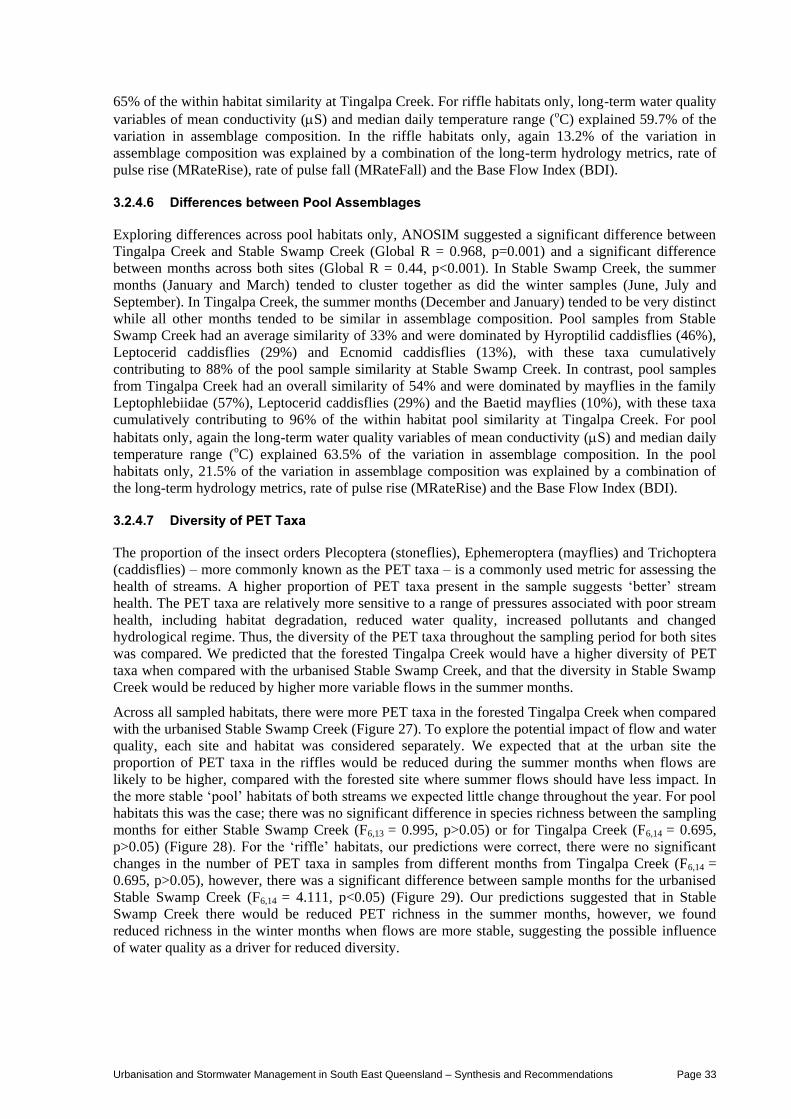
Urbanisation and Stormwater Management in South East Queensland – Synthesis and Recommendations Page 33
65% of the within habitat similarity at Tingalpa Creek. For riffle habitats only, long-term water quality
variables of mean conductivity (S) and median daily temperature range (oC) explained 59.7% of the
variation in assemblage composition. In the riffle habitats only, again 13.2% of the variation in
assemblage composition was explained by a combination of the long-term hydrology metrics, rate of
pulse rise (MRateRise), rate of pulse fall (MRateFall) and the Base Flow Index (BDI).
3.2.4.6 Differences between Pool Assemblages
Exploring differences across pool habitats only, ANOSIM suggested a significant difference between
Tingalpa Creek and Stable Swamp Creek (Global R = 0.968, p=0.001) and a significant difference
between months across both sites (Global R = 0.44, p<0.001). In Stable Swamp Creek, the summer
months (January and March) tended to cluster together as did the winter samples (June, July and
September). In Tingalpa Creek, the summer months (December and January) tended to be very distinct
while all other months tended to be similar in assemblage composition. Pool samples from Stable
Swamp Creek had an average similarity of 33% and were dominated by Hyroptilid caddisflies (46%),
Leptocerid caddisflies (29%) and Ecnomid caddisflies (13%), with these taxa cumulatively
contributing to 88% of the pool sample similarity at Stable Swamp Creek. In contrast, pool samples
from Tingalpa Creek had an overall similarity of 54% and were dominated by mayflies in the family
Leptophlebiidae (57%), Leptocerid caddisflies (29%) and the Baetid mayflies (10%), with these taxa
cumulatively contributing to 96% of the within habitat pool similarity at Tingalpa Creek. For pool
habitats only, again the long-term water quality variables of mean conductivity (S) and median daily
temperature range (oC) explained 63.5% of the variation in assemblage composition. In the pool
habitats only, 21.5% of the variation in assemblage composition was explained by a combination of
the long-term hydrology metrics, rate of pulse rise (MRateRise) and the Base Flow Index (BDI).
3.2.4.7 Diversity of PET Taxa
The proportion of the insect orders Plecoptera (stoneflies), Ephemeroptera (mayflies) and Trichoptera
(caddisflies) – more commonly known as the PET taxa – is a commonly used metric for assessing the
health of streams. A higher proportion of PET taxa present in the sample suggests ‘better’ stream
health. The PET taxa are relatively more sensitive to a range of pressures associated with poor stream
health, including habitat degradation, reduced water quality, increased pollutants and changed
hydrological regime. Thus, the diversity of the PET taxa throughout the sampling period for both sites
was compared. We predicted that the forested Tingalpa Creek would have a higher diversity of PET
taxa when compared with the urbanised Stable Swamp Creek, and that the diversity in Stable Swamp
Creek would be reduced by higher more variable flows in the summer months.
Across all sampled habitats, there were more PET taxa in the forested Tingalpa Creek when compared
with the urbanised Stable Swamp Creek (Figure 27). To explore the potential impact of flow and water
quality, each site and habitat was considered separately. We expected that at the urban site the
proportion of PET taxa in the riffles would be reduced during the summer months when flows are
likely to be higher, compared with the forested site where summer flows should have less impact. In
the more stable ‘pool’ habitats of both streams we expected little change throughout the year. For pool
habitats this was the case; there was no significant difference in species richness between the sampling
months for either Stable Swamp Creek (F6,13 = 0.995, p>0.05) or for Tingalpa Creek (F6,14 = 0.695,
p>0.05) (Figure 28). For the ‘riffle’ habitats, our predictions were correct, there were no significant
changes in the number of PET taxa in samples from different months from Tingalpa Creek (F6,14 =
0.695, p>0.05), however, there was a significant difference between sample months for the urbanised
Stable Swamp Creek (F6,14 = 4.111, p<0.05) (Figure 29). Our predictions suggested that in Stable
Swamp Creek there would be reduced PET richness in the summer months, however, we found
reduced richness in the winter months when flows are more stable, suggesting the possible influence
of water quality as a driver for reduced diversity.
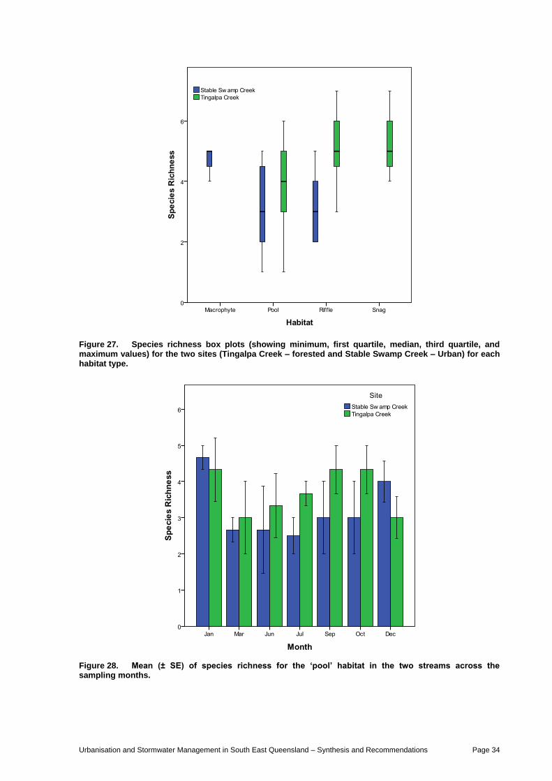
Urbanisation and Stormwater Management in South East Queensland – Synthesis and Recommendations Page 34
Figure 27. Species richness box plots (showing minimum, first quartile, median, third quartile, and maximum values) for the two sites (Tingalpa Creek – forested and Stable Swamp Creek – Urban) for each habitat type.
Figure 28. Mean (± SE) of species richness for the ‘pool’ habitat in the two streams across the sampling months.
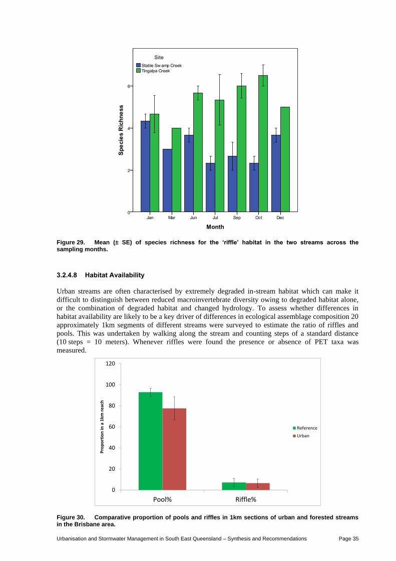
Urbanisation and Stormwater Management in South East Queensland – Synthesis and Recommendations Page 35
Figure 29. Mean (± SE) of species richness for the ‘riffle’ habitat in the two streams across the sampling months.
3.2.4.8 Habitat Availability
Urban streams are often characterised by extremely degraded in-stream habitat which can make it
difficult to distinguish between reduced macroinvertebrate diversity owing to degraded habitat alone,
or the combination of degraded habitat and changed hydrology. To assess whether differences in
habitat availability are likely to be a key driver of differences in ecological assemblage composition 20
approximately 1km segments of different streams were surveyed to estimate the ratio of riffles and
pools. This was undertaken by walking along the stream and counting steps of a standard distance
(10 steps = 10 meters). Whenever riffles were found the presence or absence of PET taxa was
measured.
0
20
40
60
80
100
120
Pool% Riffle%
Pro
po
rtio
n in
a 1
km r
eac
h
Reference
Urban
Figure 30. Comparative proportion of pools and riffles in 1km sections of urban and forested streams in the Brisbane area.
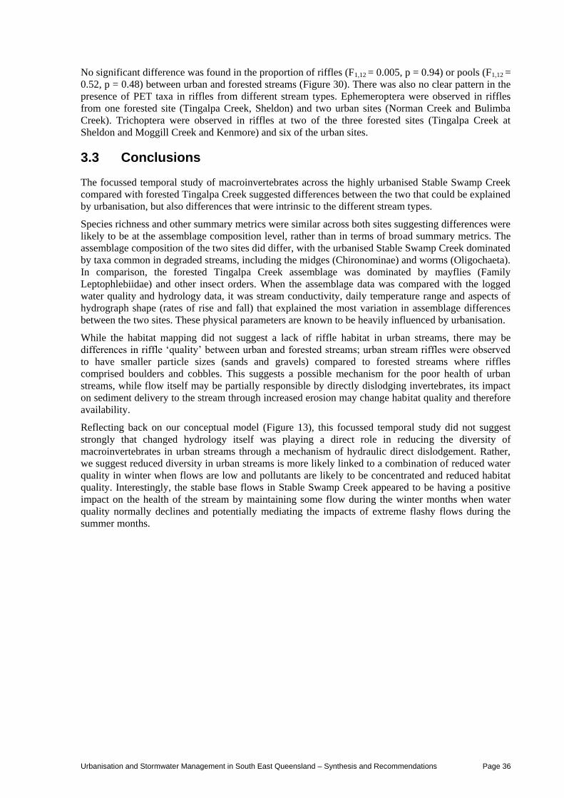
Urbanisation and Stormwater Management in South East Queensland – Synthesis and Recommendations Page 36
No significant difference was found in the proportion of riffles (F1,12 = 0.005, p = 0.94) or pools (F1,12 =
0.52, p = 0.48) between urban and forested streams (Figure 30). There was also no clear pattern in the
presence of PET taxa in riffles from different stream types. Ephemeroptera were observed in riffles
from one forested site (Tingalpa Creek, Sheldon) and two urban sites (Norman Creek and Bulimba
Creek). Trichoptera were observed in riffles at two of the three forested sites (Tingalpa Creek at
Sheldon and Moggill Creek and Kenmore) and six of the urban sites.
3.3 Conclusions
The focussed temporal study of macroinvertebrates across the highly urbanised Stable Swamp Creek
compared with forested Tingalpa Creek suggested differences between the two that could be explained
by urbanisation, but also differences that were intrinsic to the different stream types.
Species richness and other summary metrics were similar across both sites suggesting differences were
likely to be at the assemblage composition level, rather than in terms of broad summary metrics. The
assemblage composition of the two sites did differ, with the urbanised Stable Swamp Creek dominated
by taxa common in degraded streams, including the midges (Chironominae) and worms (Oligochaeta).
In comparison, the forested Tingalpa Creek assemblage was dominated by mayflies (Family
Leptophlebiidae) and other insect orders. When the assemblage data was compared with the logged
water quality and hydrology data, it was stream conductivity, daily temperature range and aspects of
hydrograph shape (rates of rise and fall) that explained the most variation in assemblage differences
between the two sites. These physical parameters are known to be heavily influenced by urbanisation.
While the habitat mapping did not suggest a lack of riffle habitat in urban streams, there may be
differences in riffle ‘quality’ between urban and forested streams; urban stream riffles were observed
to have smaller particle sizes (sands and gravels) compared to forested streams where riffles
comprised boulders and cobbles. This suggests a possible mechanism for the poor health of urban
streams, while flow itself may be partially responsible by directly dislodging invertebrates, its impact
on sediment delivery to the stream through increased erosion may change habitat quality and therefore
availability.
Reflecting back on our conceptual model (Figure 13), this focussed temporal study did not suggest
strongly that changed hydrology itself was playing a direct role in reducing the diversity of
macroinvertebrates in urban streams through a mechanism of hydraulic direct dislodgement. Rather,
we suggest reduced diversity in urban streams is more likely linked to a combination of reduced water
quality in winter when flows are low and pollutants are likely to be concentrated and reduced habitat
quality. Interestingly, the stable base flows in Stable Swamp Creek appeared to be having a positive
impact on the health of the stream by maintaining some flow during the winter months when water
quality normally declines and potentially mediating the impacts of extreme flashy flows during the
summer months.
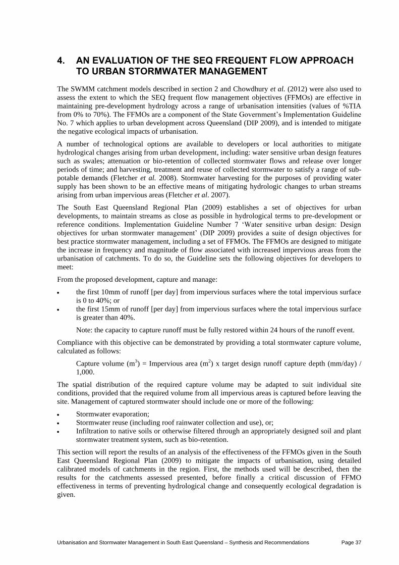
Urbanisation and Stormwater Management in South East Queensland – Synthesis and Recommendations Page 37
4. AN EVALUATION OF THE SEQ FREQUENT FLOW APPROACH TO URBAN STORMWATER MANAGEMENT
The SWMM catchment models described in section 2 and Chowdhury et al. (2012) were also used to
assess the extent to which the SEQ frequent flow management objectives (FFMOs) are effective in
maintaining pre-development hydrology across a range of urbanisation intensities (values of %TIA
from 0% to 70%). The FFMOs are a component of the State Government’s Implementation Guideline
No. 7 which applies to urban development across Queensland (DIP 2009), and is intended to mitigate
the negative ecological impacts of urbanisation.
A number of technological options are available to developers or local authorities to mitigate
hydrological changes arising from urban development, including: water sensitive urban design features
such as swales; attenuation or bio-retention of collected stormwater flows and release over longer
periods of time; and harvesting, treatment and reuse of collected stormwater to satisfy a range of sub-
potable demands (Fletcher et al. 2008). Stormwater harvesting for the purposes of providing water
supply has been shown to be an effective means of mitigating hydrologic changes to urban streams
arising from urban impervious areas (Fletcher et al. 2007).
The South East Queensland Regional Plan (2009) establishes a set of objectives for urban
developments, to maintain streams as close as possible in hydrological terms to pre-development or
reference conditions. Implementation Guideline Number 7 ‘Water sensitive urban design: Design
objectives for urban stormwater management’ (DIP 2009) provides a suite of design objectives for
best practice stormwater management, including a set of FFMOs. The FFMOs are designed to mitigate
the increase in frequency and magnitude of flow associated with increased impervious areas from the
urbanisation of catchments. To do so, the Guideline sets the following objectives for developers to
meet:
From the proposed development, capture and manage:
the first 10mm of runoff [per day] from impervious surfaces where the total impervious surface
is 0 to 40%; or
the first 15mm of runoff [per day] from impervious surfaces where the total impervious surface
is greater than 40%.
Note: the capacity to capture runoff must be fully restored within 24 hours of the runoff event.
Compliance with this objective can be demonstrated by providing a total stormwater capture volume,
calculated as follows:
Capture volume (m3) = Impervious area (m2) x target design runoff capture depth (mm/day) /
1,000.
The spatial distribution of the required capture volume may be adapted to suit individual site
conditions, provided that the required volume from all impervious areas is captured before leaving the
site. Management of captured stormwater should include one or more of the following:
Stormwater evaporation;
Stormwater reuse (including roof rainwater collection and use), or;
Infiltration to native soils or otherwise filtered through an appropriately designed soil and plant
stormwater treatment system, such as bio-retention.
This section will report the results of an analysis of the effectiveness of the FFMOs given in the South
East Queensland Regional Plan (2009) to mitigate the impacts of urbanisation, using detailed
calibrated models of catchments in the region. First, the methods used will be described, then the
results for the catchments assessed presented, before finally a critical discussion of FFMO
effectiveness in terms of preventing hydrological change and consequently ecological degradation is
given.
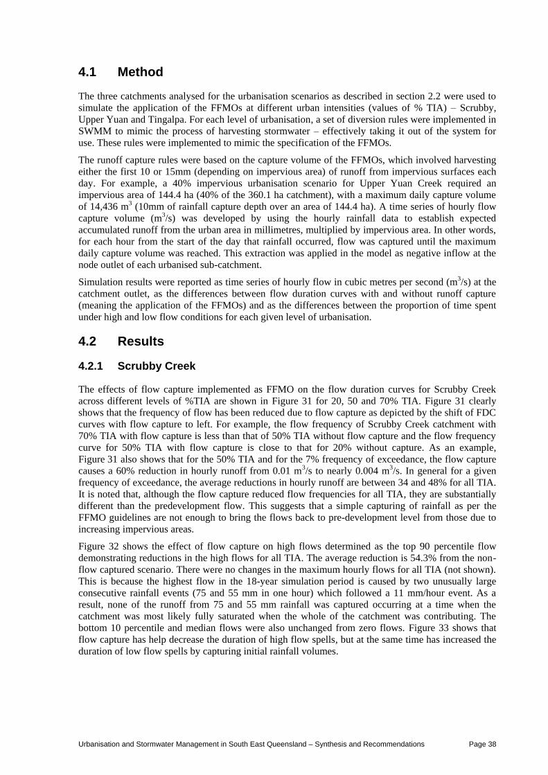
Urbanisation and Stormwater Management in South East Queensland – Synthesis and Recommendations Page 38
4.1 Method
The three catchments analysed for the urbanisation scenarios as described in section 2.2 were used to
simulate the application of the FFMOs at different urban intensities (values of % TIA) – Scrubby,
Upper Yuan and Tingalpa. For each level of urbanisation, a set of diversion rules were implemented in
SWMM to mimic the process of harvesting stormwater – effectively taking it out of the system for
use. These rules were implemented to mimic the specification of the FFMOs.
The runoff capture rules were based on the capture volume of the FFMOs, which involved harvesting
either the first 10 or 15mm (depending on impervious area) of runoff from impervious surfaces each
day. For example, a 40% impervious urbanisation scenario for Upper Yuan Creek required an
impervious area of 144.4 ha (40% of the 360.1 ha catchment), with a maximum daily capture volume
of 14,436 m3 (10mm of rainfall capture depth over an area of 144.4 ha). A time series of hourly flow
capture volume (m3/s) was developed by using the hourly rainfall data to establish expected
accumulated runoff from the urban area in millimetres, multiplied by impervious area. In other words,
for each hour from the start of the day that rainfall occurred, flow was captured until the maximum
daily capture volume was reached. This extraction was applied in the model as negative inflow at the
node outlet of each urbanised sub-catchment.
Simulation results were reported as time series of hourly flow in cubic metres per second (m3/s) at the
catchment outlet, as the differences between flow duration curves with and without runoff capture
(meaning the application of the FFMOs) and as the differences between the proportion of time spent
under high and low flow conditions for each given level of urbanisation.
4.2 Results
4.2.1 Scrubby Creek
The effects of flow capture implemented as FFMO on the flow duration curves for Scrubby Creek
across different levels of %TIA are shown in Figure 31 for 20, 50 and 70% TIA. Figure 31 clearly
shows that the frequency of flow has been reduced due to flow capture as depicted by the shift of FDC
curves with flow capture to left. For example, the flow frequency of Scrubby Creek catchment with
70% TIA with flow capture is less than that of 50% TIA without flow capture and the flow frequency
curve for 50% TIA with flow capture is close to that for 20% without capture. As an example,
Figure 31 also shows that for the 50% TIA and for the 7% frequency of exceedance, the flow capture
causes a 60% reduction in hourly runoff from 0.01 m3/s to nearly 0.004 m3/s. In general for a given
frequency of exceedance, the average reductions in hourly runoff are between 34 and 48% for all TIA.
It is noted that, although the flow capture reduced flow frequencies for all TIA, they are substantially
different than the predevelopment flow. This suggests that a simple capturing of rainfall as per the
FFMO guidelines are not enough to bring the flows back to pre-development level from those due to
increasing impervious areas.
Figure 32 shows the effect of flow capture on high flows determined as the top 90 percentile flow
demonstrating reductions in the high flows for all TIA. The average reduction is 54.3% from the non-
flow captured scenario. There were no changes in the maximum hourly flows for all TIA (not shown).
This is because the highest flow in the 18-year simulation period is caused by two unusually large
consecutive rainfall events (75 and 55 mm in one hour) which followed a 11 mm/hour event. As a
result, none of the runoff from 75 and 55 mm rainfall was captured occurring at a time when the
catchment was most likely fully saturated when the whole of the catchment was contributing. The
bottom 10 percentile and median flows were also unchanged from zero flows. Figure 33 shows that
flow capture has help decrease the duration of high flow spells, but at the same time has increased the
duration of low flow spells by capturing initial rainfall volumes.
Urbanisation and Stormwater Management in South East Queensland – Synthesis and Recommendations Page 39
Figure 31. Effect of flow capture on flow duration curve for increasing TIA for Scrubby Creek. Plots for only 20, 50 and 70 percent TIA are shown for clarity.
Figure 32. Effect of flow capture implemented as frequent flow management option (FFMO) on top 90 percentile flow in the Scrubby Creek catchment.
Figure 33. Effect of flow capture on the (left) high flow and (right) low flow duration in Scrubby Creek catchment.
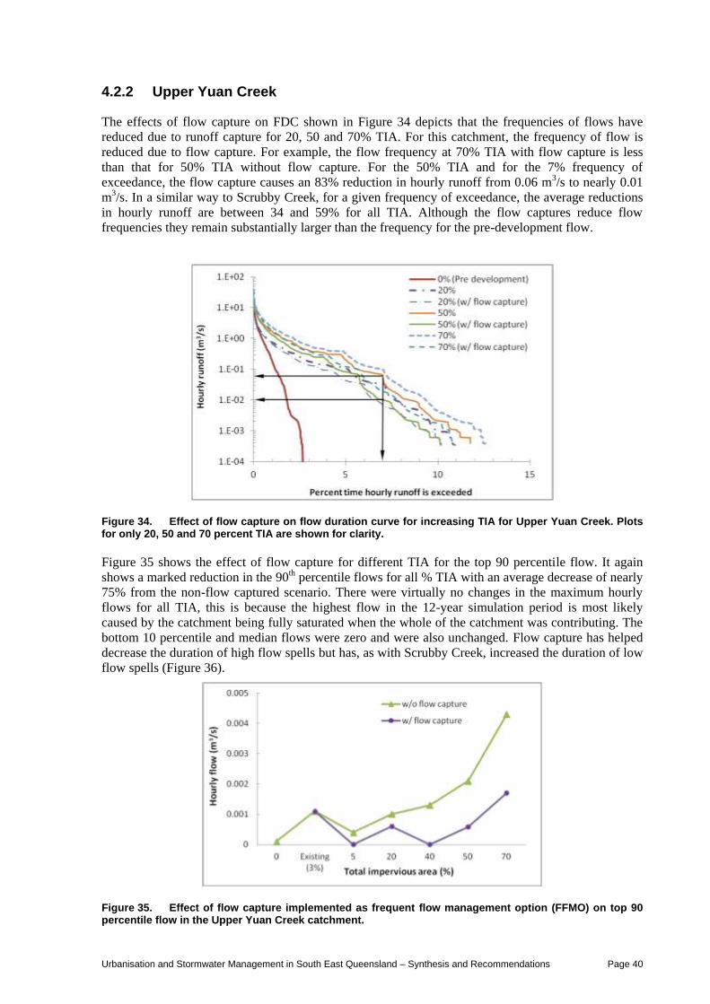
Urbanisation and Stormwater Management in South East Queensland – Synthesis and Recommendations Page 40
4.2.2 Upper Yuan Creek
The effects of flow capture on FDC shown in Figure 34 depicts that the frequencies of flows have
reduced due to runoff capture for 20, 50 and 70% TIA. For this catchment, the frequency of flow is
reduced due to flow capture. For example, the flow frequency at 70% TIA with flow capture is less
than that for 50% TIA without flow capture. For the 50% TIA and for the 7% frequency of
exceedance, the flow capture causes an 83% reduction in hourly runoff from 0.06 m3/s to nearly 0.01
m3/s. In a similar way to Scrubby Creek, for a given frequency of exceedance, the average reductions
in hourly runoff are between 34 and 59% for all TIA. Although the flow captures reduce flow
frequencies they remain substantially larger than the frequency for the pre-development flow.
Figure 34. Effect of flow capture on flow duration curve for increasing TIA for Upper Yuan Creek. Plots for only 20, 50 and 70 percent TIA are shown for clarity.
Figure 35 shows the effect of flow capture for different TIA for the top 90 percentile flow. It again
shows a marked reduction in the 90th percentile flows for all % TIA with an average decrease of nearly
75% from the non-flow captured scenario. There were virtually no changes in the maximum hourly
flows for all TIA, this is because the highest flow in the 12-year simulation period is most likely
caused by the catchment being fully saturated when the whole of the catchment was contributing. The
bottom 10 percentile and median flows were zero and were also unchanged. Flow capture has helped
decrease the duration of high flow spells but has, as with Scrubby Creek, increased the duration of low
flow spells (Figure 36).
Figure 35. Effect of flow capture implemented as frequent flow management option (FFMO) on top 90 percentile flow in the Upper Yuan Creek catchment.
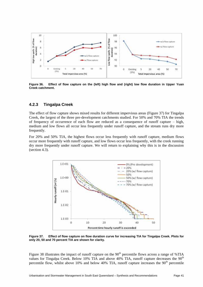
Urbanisation and Stormwater Management in South East Queensland – Synthesis and Recommendations Page 41
Figure 36. Effect of flow capture on the (left) high flow and (right) low flow duration in Upper Yuan Creek catchment.
4.2.3 Tingalpa Creek
The effect of flow capture shows mixed results for different impervious areas (Figure 37) for Tingalpa
Creek, the largest of the three pre-development catchments studied. For 50% and 70% TIA the trends
of frequency of occurrence of each flow are reduced as a consequence of runoff capture – high,
medium and low flows all occur less frequently under runoff capture, and the stream runs dry more
frequently.
For 20% and 50% TIA, the highest flows occur less frequently with runoff capture, medium flows
occur more frequently with runoff capture, and low flows occur less frequently, with the creek running
dry more frequently under runoff capture. We will return to explaining why this is in the discussion
(section 4.3).
Figure 37. Effect of flow capture on flow duration curve for increasing TIA for Tingalpa Creek. Plots for only 20, 50 and 70 percent TIA are shown for clarity.
Figure 38 illustrates the impact of runoff capture on the 90th percentile flows across a range of %TIA
values for Tingalpa Creek. Below 10% TIA and above 40% TIA, runoff capture decreases the 90th
percentile flow, whilst above 10% and below 40% TIA, runoff capture increases the 90th percentile
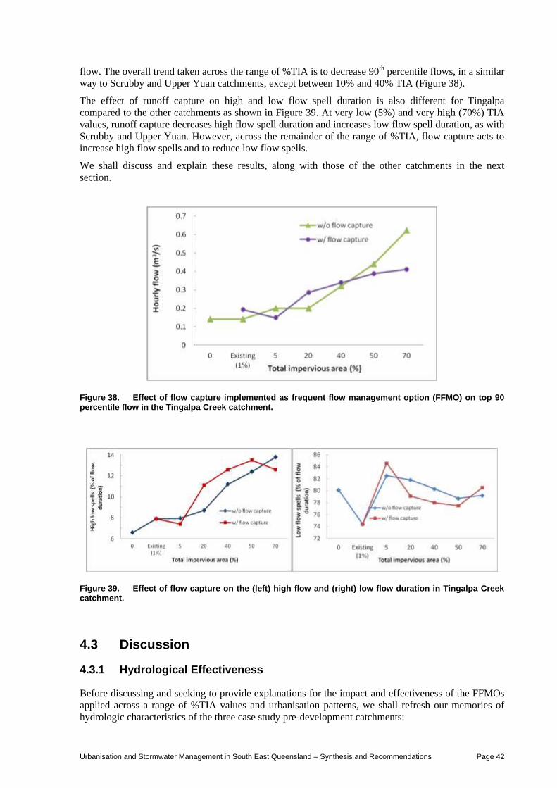
Urbanisation and Stormwater Management in South East Queensland – Synthesis and Recommendations Page 42
flow. The overall trend taken across the range of %TIA is to decrease 90th percentile flows, in a similar
way to Scrubby and Upper Yuan catchments, except between 10% and 40% TIA (Figure 38).
The effect of runoff capture on high and low flow spell duration is also different for Tingalpa
compared to the other catchments as shown in Figure 39. At very low (5%) and very high (70%) TIA
values, runoff capture decreases high flow spell duration and increases low flow spell duration, as with
Scrubby and Upper Yuan. However, across the remainder of the range of %TIA, flow capture acts to
increase high flow spells and to reduce low flow spells.
We shall discuss and explain these results, along with those of the other catchments in the next
section.
Figure 38. Effect of flow capture implemented as frequent flow management option (FFMO) on top 90 percentile flow in the Tingalpa Creek catchment.
Figure 39. Effect of flow capture on the (left) high flow and (right) low flow duration in Tingalpa Creek catchment.
4.3 Discussion
4.3.1 Hydrological Effectiveness
Before discussing and seeking to provide explanations for the impact and effectiveness of the FFMOs
applied across a range of %TIA values and urbanisation patterns, we shall refresh our memories of
hydrologic characteristics of the three case study pre-development catchments:
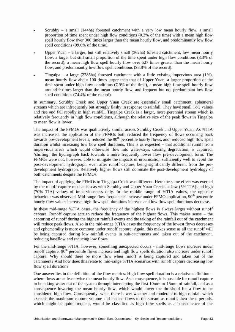
Urbanisation and Stormwater Management in South East Queensland – Synthesis and Recommendations Page 43
Scrubby – a small (144ha) forested catchment with a very low mean hourly flow, a small
proportion of time spent under high flow conditions (0.3% of the time) with a mean high flow
spell hourly flow over 300 times larger than the mean hourly flow, and predominantly low flow
spell conditions (99.6% of the time).
Upper Yuan – a larger, but still relatively small (362ha) forested catchment, low mean hourly
flow, a larger but still small proportion of the time spent under high flow conditions (3.3% of
the record), a mean high flow spell hourly flow over 527 times greater than the mean hourly
flow, and predominantly low flow spell conditions (93.8% of the record).
Tingalpa – a large (2785ha) forested catchment with a little existing impervious area (1%),
mean hourly flow about 100 times larger than that of Upper Yuan, a larger proportion of the
time spent under high flow conditions (7.9% of the time), a mean high flow spell hourly flow
around 9 times larger than the mean hourly flow, and frequent but not predominant low flow
spell conditions (74.4% of the record).
In summary, Scrubby Creek and Upper Yuan Creek are essentially small catchment, ephemeral
streams which are infrequently but strongly flashy in response to rainfall. They have small ToC values
and rise and fall rapidly in high rainfall. Tingalpa Creek is a larger, more perennial stream which is
relatively frequently in high flow conditions, although the relative size of the peak flows in Tingalpa
to mean flow is lower.
The impact of the FFMOs was qualitatively similar across Scrubby Creek and Upper Yuan. As %TIA
was increased, the application of the FFMOs both reduced the frequency of flows occurring back
towards pre-development levels; reduced the 90th percentile hourly flows, and; reduced high flow spell
duration whilst increasing low flow spell durations. This is as expected – that additional runoff from
impervious areas which would otherwise flow into waterways, causing degradation, is captured,
‘shifting’ the hydrograph back towards a more frequently lower flow pre-development form. The
FFMOs were not, however, able to mitigate the impacts of urbanisation sufficiently well to avoid the
post-development hydrograph, even after runoff capture, being significantly different from the pre-
development hydrograph. Relatively higher flows still dominate the post-development hydrology of
both catchments despite the FFMOs.
The impact of applying the FFMOs to Tingalpa Creek was different. Here the same effect was exerted
by the runoff capture mechanism as with Scrubby and Upper Yuan Creeks at low (5% TIA) and high
(70% TIA) values of imperviousness only. In the middle range of %TIA values, the opposite
behaviour was observed. Mid-range flow frequencies increase under FFMO application, 90th percentile
hourly flow values increase, high flow spell durations increase and low flow spell durations decrease.
In these mid-range %TIA cases, the frequency of the highest flows is always larger without runoff
capture. Runoff capture acts to reduce the frequency of the highest flows. This makes sense – the
capturing of runoff during the highest rainfall events and the taking of the rainfall out of the catchment
will reduce peak flows. Also in the mid-range %TIA cases the frequency of the lowest flows decreases
and ephemerality is more common under runoff capture. Again, this makes sense as all the runoff will
be being captured during low rainfall events in sub-catchments and taken out of the catchment,
reducing baseflow and reducing low flows.
For the mid-range %TIA, however, something unexpected occurs - mid-range flows increase under
runoff capture, 90th percentile flows increase and high flow spells duration also increase under runoff
capture. Why should there be more flow when runoff is being captured and taken out of the
catchment? And how does this relate to mid-range %TIA scenarios with runoff capture decreasing low
flow spell duration?
One answer lies in the definition of the flow metrics. High flow spell duration is a relative definition –
where flows are at least twice the mean hourly flow. As a consequence, it is possible for runoff capture
to be taking water out of the system through intercepting the first 10mm or 15mm of rainfall, and as a
consequence lowering the mean hourly flow, which would lower the threshold for a flow to be
considered high flow. Consequently, when there is wet weather and moderate to high rainfall which
exceeds the maximum capture volume and instead flows to the stream as runoff, then these periods,
which might be quite frequent, would be classified as high flow spells as a consequence of the
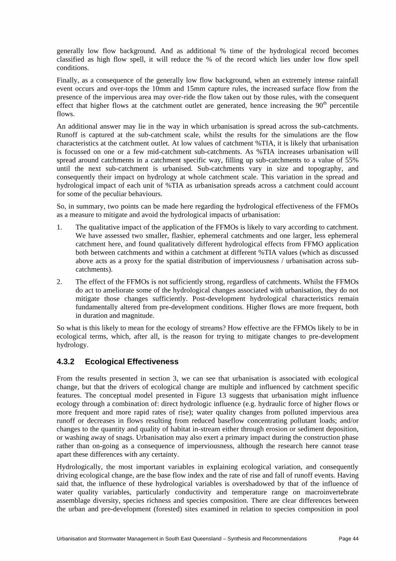
Urbanisation and Stormwater Management in South East Queensland – Synthesis and Recommendations Page 44
generally low flow background. And as additional % time of the hydrological record becomes
classified as high flow spell, it will reduce the % of the record which lies under low flow spell
conditions.
Finally, as a consequence of the generally low flow background, when an extremely intense rainfall
event occurs and over-tops the 10mm and 15mm capture rules, the increased surface flow from the
presence of the impervious area may over-ride the flow taken out by those rules, with the consequent
effect that higher flows at the catchment outlet are generated, hence increasing the 90th percentile
flows.
An additional answer may lie in the way in which urbanisation is spread across the sub-catchments.
Runoff is captured at the sub-catchment scale, whilst the results for the simulations are the flow
characteristics at the catchment outlet. At low values of catchment %TIA, it is likely that urbanisation
is focussed on one or a few mid-catchment sub-catchments. As %TIA increases urbanisation will
spread around catchments in a catchment specific way, filling up sub-catchments to a value of 55%
until the next sub-catchment is urbanised. Sub-catchments vary in size and topography, and
consequently their impact on hydrology at whole catchment scale. This variation in the spread and
hydrological impact of each unit of %TIA as urbanisation spreads across a catchment could account
for some of the peculiar behaviours.
So, in summary, two points can be made here regarding the hydrological effectiveness of the FFMOs
as a measure to mitigate and avoid the hydrological impacts of urbanisation:
1. The qualitative impact of the application of the FFMOs is likely to vary according to catchment.
We have assessed two smaller, flashier, ephemeral catchments and one larger, less ephemeral
catchment here, and found qualitatively different hydrological effects from FFMO application
both between catchments and within a catchment at different %TIA values (which as discussed
above acts as a proxy for the spatial distribution of imperviousness / urbanisation across sub-
catchments).
2. The effect of the FFMOs is not sufficiently strong, regardless of catchments. Whilst the FFMOs
do act to ameliorate some of the hydrological changes associated with urbanisation, they do not
mitigate those changes sufficiently. Post-development hydrological characteristics remain
fundamentally altered from pre-development conditions. Higher flows are more frequent, both
in duration and magnitude.
So what is this likely to mean for the ecology of streams? How effective are the FFMOs likely to be in
ecological terms, which, after all, is the reason for trying to mitigate changes to pre-development
hydrology.
4.3.2 Ecological Effectiveness
From the results presented in section 3, we can see that urbanisation is associated with ecological
change, but that the drivers of ecological change are multiple and influenced by catchment specific
features. The conceptual model presented in Figure 13 suggests that urbanisation might influence
ecology through a combination of: direct hydrologic influence (e.g. hydraulic force of higher flows or
more frequent and more rapid rates of rise); water quality changes from polluted impervious area
runoff or decreases in flows resulting from reduced baseflow concentrating pollutant loads; and/or
changes to the quantity and quality of habitat in-stream either through erosion or sediment deposition,
or washing away of snags. Urbanisation may also exert a primary impact during the construction phase
rather than on-going as a consequence of imperviousness, although the research here cannot tease
apart these differences with any certainty.
Hydrologically, the most important variables in explaining ecological variation, and consequently
driving ecological change, are the base flow index and the rate of rise and fall of runoff events. Having
said that, the influence of these hydrological variables is overshadowed by that of the influence of
water quality variables, particularly conductivity and temperature range on macroinvertebrate
assemblage diversity, species richness and species composition. There are clear differences between
the urban and pre-development (forested) sites examined in relation to species composition in pool
Urbanisation and Stormwater Management in South East Queensland – Synthesis and Recommendations Page 45
habitats and in riffle habitats, but not overall. There are also clear differences over time, between the
wet period (summer) and the dry period (winter) when runoff varies significantly.
Given the hydrologic impact of applying the FFMOs as described in the assessment presented in this
section we can say with reasonable certainty that the ecological benefits of applying the FFMOs:
1. will vary with the catchments involved, as smaller, more ephemeral catchments do not behave
hydrologically in line with larger, less ephemeral catchments under urbanisation or under runoff
capture;
2. will not be of a sufficient magnitude to avoid degradation from pre-development conditions; and
3. cannot be clearly identified without a knowledge of how they will impact on water quality
variables.
Reductions in the higher flows and in the proportion of time spent under high flow conditions
following the application of FFMOs in smaller catchments may help ensure habitat quality doesn’t
degrade through pool or riffle sedimentation. This might help maintain pre-development species
composition. Applying the FFMOs will increase the proportion of time spent under low flow
conditions and return smaller catchments towards greater ephemerality. Ecologically, this will have an
impact, but what, is unclear. Baseflow index was found to be a significant influence on species
composition within macroinvertebrate assemblages. This may be as function of baseflow being a
determinant of significant water quality variables such as conductivity and temperature range.
Urbanisation for smaller, more ephemeral catchments is likely to result in increases in the frequency of
all flows, and a reduction in overall ephemerality. This will change the species composition of
assemblages but how is not clear. PET (sensitive) taxa presence were found to be likely to be affected
by maintained baseflow over winter, a feature which may be promoted by urbanisation in flashy
catchments, depending on how it is implemented. The application of FFMOs reduced the frequency of
all flows towards pre-development, but not strongly enough. As a consequence the application of the
FFMOs may have negative water quality impacts (increased temperature ranges).
The ecological impact of applying the FFMOs to larger catchments is more complicated and less clear,
being influenced by the spatial pattern and intensity of urban development across sub-catchments. At
low (5% TIA) and high (70% TIA) intensities of urbanisation, the application of FFMOs does as just
described for smaller catchments – reducing higher flows, reducing the time spent under high flow
conditions and increasing the time spent under low flow conditions. This may be good ecologically for
the reasons stated above, but for most of the range of TIA intensities (>5% and <70%) the application
of FFMOs has different consequences. Here, mid-flow frequencies increase, high flow spell durations
increase and low flow spell durations decrease. This latter feature could have significant impacts
ecologically depending on what the decrease in time spent under low flow conditions would mean for
water quality. If the mean daily temperature range decreases then there are likely to be ecological
benefits in terms of promoting greater diversity and PET taxa abundance. And simply spending less
time under low flow conditions following runoff capture may provide a way of supporting sensitive
taxa as seen with PET species presence at Stable Swamp Creek.
In summary then, the ecological consequences of applying the FFMOs as currently defined are unclear
except that we can say they will not maintain catchments in their pre-development hydrological, and
consequently ecological, condition. It appears that water quality variables are more important
ecological determinants in SEQ than flow component changes and greater knowledge is needed about
how flow relates to water quality and consequently ecological assemblages. Reducing low flow spell
durations and maintaining good base flows, as can happen in the mid-range of urbanisation intensities
in larger catchments can help promote positive ecological structure and function even in intensely
urbanised areas.
Urbanisation and Stormwater Management in South East Queensland – Synthesis and Recommendations Page 46
5. CONCLUSIONS AND RECOMMENDATIONS
We positioned this report to provide a synthesis of the research results from the project concerning the
hydrological and ecological impacts of urbanisation in SEQ. Acknowledging the existing but largely
temperate climate based literature on these impacts of urbanisation, we were motivated in part to
characterise how urbanisation influences hydrology and ecology in a sub-tropical climatic setting. We
set out to answer the following questions in this report:
1. How does the imperviousness of urban areas influence the hydrology and ecology of streams in
South East Queensland?
2. How effective is the current frequent flow management objective approach to managing the
hydrological and ecological impacts of urbanisation in South East Queensland?
3. What recommendations for action and what gaps in knowledge are suggested by the research in
relation to urban stormwater management in South East Queensland?
We will turn our attention immediately to answering questions 1 and 2 and to then answering question
3 in the sub-sections which follow.
From the hydrological results presented in section 2 and section 3 we can see that urbanisation is
clearly associated with changes in hydrology. We can also see that those changes are complex and
whilst there are some generalities (increases in high flow condition duration, increases in mean flow
and 90th percentile flow, increases in the frequency and rate of runoff event rise), the hydrological
impact of urbanisation depends on catchment characteristics including size, slope, ToC, sub-catchment
sizes and distributions, and on the pattern of urbanisation itself across sub-catchments and the
catchment as a whole. The same urbanisation pattern can exert a qualitatively different impact
hydrologically depending on the composition of the whole catchment in terms of sub-catchments.
Maximum hourly flows appear not to be impacted by urbanisation, but 90th percentile hourly flows
and mean hourly flows are impacted, both increasing with urbanisation. The number of runoff events
increases with urbanisation and the size of the rise and fall in flow with each event also rises with
urbanisation.
The proportion of time spent under high flow conditions tends to increase with urbanisation for any
given catchment, but necessarily so – there can be some catchment specific decreases in high flow
spell duration under urbanisation, depending on sub-catchment characteristics. The mean of high flow
spells may increase, but not necessarily so. The proportion of time spent under low flow conditions
tends to decrease with urbanisation, probably as a consequence of the streams studied being ephemeral
in their pre-development state rather than strongly base flow supported and perennial. Such streams
respond to smaller rainfall events when urbanised, events which instead of simply infiltrating into the
soil and percolating away, result in impervious surface runoff which feeds stream flow. However, the
decrease in low flow spell duration looks more likely to be true of smaller, flashier, more ephemeral
catchments, with larger catchments like Tingalpa, showing an initial (up to 5% TIA) increase in low
flow spell duration (associated perhaps with a decrease in infiltration and baseflow), and then a
decrease in the proportion of time spent under low flow conditions for %TIA values greater than 5%.
This may again be a consequence of imperviousness enabling smaller rainfall events to directly impact
stream flow, whereas under pre-development conditions, small events would simply infiltrate away
and not contribute at all to stream flow.
How do these kinds of changes impact on the ecology of urban streams in SEQ? First of all, it is
important to note that the research here clearly indicates that there are negative aquatic ecological
impacts associated with urbanisation in SEQ. In particular, the EHMP analysis described in section 3
demonstrates that urbanisation (as a lumped land use category) is associated with decreases in
macroinvertebrate richness, and increase in the proportion of alien fish species observed. TIA, either
lumped or weighted to mimic the effect of DCIA was not observed to exert a strong impact on any
ecological variables, although it was observed to have an influence on the proportion of native to alien
fish species observed. Other land uses were observed to have a strong ecological influence. For
Urbanisation and Stormwater Management in South East Queensland – Synthesis and Recommendations Page 47
example, forest cover was associated positively with SIGNAL score, indicating that forested land use,
particularly near rivers, is associated with the presence of more sensitive macroinvertebrate species.
The results tend to indicate that the hydrological changes following urbanisation are not significant
degrading factors in themselves. Indeed, in both the EHMP analysis and the focussed temporal case
study research, the influence of water quality variables, particularly temperature range was found to be
important. The EHMP analysis suggested DO and pH to also play an important role in determining
macroinvertebrate richness, SIGNAL and in indicators related to the abundance of native vs. alien fish
species. The temporal case study analysis suggested that conductivity and temperature range were the
most important water quality variables, in relation to determining macroinvertebrate assemblage
species composition in both pool and riffle habitats. The association of lumped urban land use with
ecological impact and the simultaneous lack of ecological impact associated with IA (TIA or proxied
DCIA) raises the question as to whether the process of urbanisation, i.e. the process of construction, is
the primary source of ecologically degrading waterway impact in SEQ, rather than the on-going
impact of impervious area runoff flows.
Whilst urban and pre-development streams had similar levels of macroinvertebrate species richness
and diversity, and similar distributions of habitat availability (riffle and pool proportions), there were
significant differences over time (seasonally) within each stream type and between each stream type in
relation to species composition. The urban stream was found to have a macroinvertebrate assemblage
with less PET (sensitive) taxa, and more dominated by midges (Chironominae) and worms
(Oligochaeta). In comparison, the pre-development, forested stream assemblage was dominated by
mayflies (family Leptophlebiidae) and other insect orders. Urban catchment pools were observed to be
poorer in habitat quality, with greater sedimentation than pre-development pools suggesting a potential
mechanism influencing species composition.
Pool species composition in both urban and pre-development streams was found to be stable over
time, i.e., not affected by higher summer or lower winter flows. Conversely, riffle species composition
in the urban stream was found to vary significantly over time, with lower diversity in the lower flow
winter months, suggesting the importance of water quality changes rather than flow changes as a
driver of assemblage change.
As with hydrological impact, the mechanisms of ecological change from urbanisation are complicated
and based on partly catchment specific features, e.g., the winter flow supporting upstream wetlands in
Stable Swamp Creek and the ecologically locally devastating iron floc problems at Blunder Creek.
The evaluation of the Qld FFMOs suggests that whilst they will be effective to a degree, bringing
hydrographs back towards their pre-development profile, they are insufficiently strong. The FFMOs
will also have an effect which is partly dependent on catchment characteristics, the distribution and
sizes of sub-catchments and the spatial pattern of urbanisation. Given the seeming lower importance of
hydrological variables on ecological structure in streams as indicated by this research, one might
question whether the FFMOs are the tool of primary importance with regards mitigating the impacts of
urbanisation on waterway ecological health.
Having provided this summary and set of conclusions about the research taken as a whole, what can be
recommended regarding policy, management and further research? The sub-sections below provide a
response.
5.1 Develop with the Catchment in Mind
One of the strongest results from the research conducted is highlighting how important catchment
specific features are in determining hydrological change outcomes from urbanisation, and how the
spatial pattern of urbanisation itself across the sub-catchments within a catchment is critically
important in determining how flow changes. The implications of this insight are that each catchment
requires a catchment specific hydrological assessment to inform the selection, design and
implementation of appropriate measures to avoid significantly changing. This raises clear practicality
issues – given the minimum time (around three years) involved to gather good quality hydrologic data
to provide reliable model calibration and validation outcomes, requiring developers, Councils or the
State to have such knowledge for each catchment is not realistic. However, we know that without such
Urbanisation and Stormwater Management in South East Queensland – Synthesis and Recommendations Page 48
knowledge the hydrological impacts arising from development may be significant with respect to pre-
development hydrology, and potentially unexpected. What can be done?
The ELOHA approach was developed to help simplify the task providing scientifically reliable but
cost and time realistic environmental flow management advice for rivers (Arthington et al. 2006, Poff
et al. 2009). Some key principles underlying ELOHA, which will not be described here as a method
(see previous references), are that hydrologically similar catchments will have similar aquatic
ecologies; and respond hydrologically and ecologically in similar ways to similar urbanisation
processes (patterns, extents, intensities). Consequently, if the rivers and streams in a given region can
be described in terms of a smaller number of hydrologic reference or pre-development condition types,
there is an opportunity to provide meaningful advice on how urbanisation ought best to be planned and
managed to avoid significant change in ecologically relevant flow variables. If a classification of
hydrologically and ecologically similar river or stream types could be developed for SEQ and the
impacts of a range of urbanisation processes teased out for each river or stream type, there would be a
sound basis for understanding how to mitigate or avoid the hydrological and ecological impacts
expected in any given catchment without the need for developing a new, empirically robust and
detailed hydrological model for every catchment. Doing so might seem like an overwhelmingly large
task, but such classification work has been undertaken for the whole of Australia at continental scale
(see Kennard et al. 2010), setting a clear precedent that such work is feasible.
Complementary to this recommended work is the need to ensure that catchment urbanisation processes
are impact assessed at both sub-catchment and whole of catchment scales. Whilst there is a clear logic
in managing stormwater runoff from impervious areas at source (the sub-catchment), the results
presented here suggest that completely mitigating additional flows will be difficult (e.g. FFMOs not
strong enough) and that the aggregate impact of urbanisation across multiple sub-catchments may be
unexpected and multiplicative. There may be a need to think about directing urbanisation towards sub-
catchments in a catchment which would minimise overall impact as assessed. At the very least sub-
catchments, which may be sizeable, cannot be treated as separate units.
5.2 Focus on Maintaining Winter Flows, In-Stream Habitat and Riparian Zones
Hydrologic variables have some influence over urban stream ecology, particularly the rate of rise and
fall of runoff events, and the frequency of those events. But water quality variables appear to explain a
greater proportion of the variability between urban and non-urban catchment aquatic ecosystem health.
In particular, the daily temperature range and conductivity were found to be of importance with
regards pool and riffle habitat species composition. Further, the reduced presence of PET taxa in the
urban site in the lower rainfall, lower flow winter indicates that water quality rather than hydrologic
influence is key. Finally, whilst the proportion of riffles and pools are similar across urban and pre-
development areas, the quality of pool habitats is suspected as being a reason as to why the urban
stream species composition was dominated by midges and worms rather than PET and other insect
taxa.
Some management recommendations arise out of these results – investing in riparian vegetation will
provide a means of reducing daily temperature maxima and ranges. This will have ecological benefits
in terms of promoting pre-development species compositions in urban streams. Further, investing in
maintaining winter flows in urban areas such that they do not reduce as much as they might under
increased imperviousness and reduced baseflow, will help ameliorate water quality degradation and
the impacts this will have on species composition. As with Stable Swamp Creek, this might be done
by means of wetlands positioned regularly down a catchment to support winter flows, and provide
summer month storage and flow retention benefits (for flooding and ecological health). Ensuring that
erosion and sediment loads are reduced will help avoid the reduction in habitat, particularly pool
habitat, which is suspected from these results as being a key driver of macroinvertebrate species
composition degradation.
Urbanisation and Stormwater Management in South East Queensland – Synthesis and Recommendations Page 49
5.3 Clarify the Relative Impacts of Construction vs. Urban Impervious Area on Waterway Ecological Health
Finally, rather than assuming that urban stream ecological degradation occurs as a consequence of on-
going pressure from impervious area runoff, it will be worth asking the question – does most of the
negative ecological impact from urbanisation occur during or shortly after the process of construction?
Assuming that the primary degrading force is on-going runoff points towards management by means
of water sensitive urban design features, and careful planning of urban layout and imperviousness. If
however, the primary impacts occur during or shortly after construction, then management by means
of improved sediment erosion control, changes to the way land is cleared, built on and then re-
vegetated might be more effective.
The EHMP based analysis showed impervious area, TIA or DCIA, had little or no impact ecologically,
whilst the presence of urban areas (treated uniformly or weighted to have urban areas closer to streams
weighted higher) had a significant degrading effect on fish populations and macroinvertebrate
assemblages. It was not clear from this research why this should be so, given the weight of evidence
from other studies on the ecological importance of DCIA in particular, but IA more generally.
Knowledge here is scant in the literature, so there is a need to monitor and assess the hydrological,
water quality and ecological changes which occur during and after urban development. This would
need to be done through detailed monitoring and analysis of one or more urban development
construction processes from the point of clearing and land preparation through building and into the
first year or two of inhabitation. The results would be revealing and could qualitatively change the
focus of urban stormwater management for ecological outcomes.
Urbanisation and Stormwater Management in South East Queensland – Synthesis and Recommendations Page 50
REFERENCES
Arthington, A. H., Bunn, S. E., Poff, N. L. and Naiman, R. J. (2006). The challenge of providing
environmental flow rules to sustain river ecosystems, Ecological Applications, 16 (4): 1311-1318.
Ashbolt, S., McIntosh, B.S., Gardiner, R., Chowdhury, R., Gardner, T., Aryal, S., Maheepala, S. and
Sheldon, F. (2012). Can stormwater harvesting restore pre-development flows in urban catchments
in South East Queensland? In Begbie, D.K., Kenway, S.J., Biermann, S.M. and Wakem, S.L. (eds)
(2012). Science Forum and Stakeholder Engagement: Building Linkages, Collaboration and Science
Quality, Urban Water Security Research Alliance, 19-20 June, 2012 Brisbane, Queensland.
Ashbolt, S., Aryal, S., Petrone, K., McIntosh, B.S., Maheepala, S., Chowdhury, R. and Gardner, T. (2013).
Can stormwater harvesting restore pre-development flows in urban catchments in South East
Queensland?, Water Science and Technology 67(2): 446–451.
Bunn, S.E., Abal, E.G., Smith, M.J., Choy, S.C., Fellows, C.S., Harch, B.D., Kennard, M.J. and Sheldon, F.
(2010), Integration of science and monitoring of river ecosystem health to guide investments in
catchment protection and rehabilitation, Freshwater Biology 55 (Suppl. 1):223-240.
Burns, M., Fletcher, T., Walsh, C.J., Ladson, A.R. and Hatt, B.E. (2012). Hydrologic shortcomings of
conventional urban stormwater management and opportunities for reform, Landscape and Urban
Planning 105: 230-240.
Chowdhury, R., Gardner, T., Gardiner, R., Hartcher, M., Aryal, S., Ashbolt, S., Petrone, K., Tonks, M.,
Ferguson, B., Maheepala, S. and McIntosh, B.S. (2012). SEQ Catchment modelling for stormwater
harvesting research: instrumentation and hydrological model calibration and validation, Urban Water
Security Research Alliance Technical Report No. 83.
DIP (2009). South East Queensland Regional Plan 2009-2031, Implementation Guideline No. 7, Water
sensitive urban design: Design objectives for urban stormwater management, Department of
Infrastructure and Planning, Queensland Government, Brisbane.
Fletcher, T., Andrieu, H. and Hamel, P. (2013). Understanding, management and modelling of urban
hydrology and its consequences for receiving waters: A state of the art, Advances in Water
Resources 51: 261-279.
Fletcher, T., Mitchell, V.G., Deletic, A., Ladson, T.R. and Sèven, A. (2007). Is stormwater harvesting
beneficial to urban waterway environmental flows, Water Science & Technology 55(4), 265-272.
Fletcher, T.D., Deletic, A., Mitchell, G.V. and Hatt, B.E. (2008). Reuse of Urban Runoff in Australia: A
Review of Recent Advances and Remaining Challenges, Journal of Environmental Quality 37(5),
116-127.
Hall, T. (2010). The Life and Death of the Australian Backyard, CSIRO Publishing, Collingwood,
Australia.
Jacobson, C.R. (2011). Identification and quantification of the hydrological impacts of imperviousness in
urban catchments: A review, Journal of Environmental Management, 92(6), 1438-1448.
Kennard, M.J., Pusey, B.J., Olden, J.D., MacKay, S.J., Stein, J.L. and Marsh, N. (2010). Classification of
natural flow regimes in Australia to support environmental flow management, Freshwater Biology
55:171-193.
OESR (2011a). Population growth highlights and trends 2011, Office of Economic and Statistical
Research, Queensland Treasury, Queensland State Government, Brisbane.
http://www.oesr.qld.gov.au/products/publications/pop-growth-highlights-trends-qld/pop-growth-highlights-trends-qld-2011.pdf.
OESR (2011b). Queensland Government population projections to 2013: Local Government areas, Office
of Economic and Statistical Research, Queensland Treasury, Queensland State Government,
Brisbane. http://www.oesr.qld.gov.au/products/publications/qld-govt-pop-proj-lga/qld-govt-pop-proj-lga-2011-edn.pdf.
Paul, M.J. and Meyer. J.L. (2001), Streams in the urban landscape. Annual Review of Ecology and
Systematics 32:333-365.
Peterson, E.E., Sheldon, F., Darnell, R., Bunn, S.E., and Harch, B.D. (2011), A comparison of spatially
explicit landscape representation methods and their relationship to stream condition. Freshwater
Biology 56:590-610.
Poff, N. L., Richter, B., Arthington, A. H., Bunn, S. E., Naiman, R. J., Kendy, E., Acreman, M., Apse, C.,
Bledsoe, B. P., Freeman, M., Henriksen, J., Jacobson, R. B., Kennen, J., Merritt, D. M., O'Keefe, J.,
Olden, J., Rogers, K., Tharme, R. E. and Warner, A. (2009). The Ecological Limits of Hydrologic
Alteration (ELOHA): A new framework for developing regional environmental flow standards,
Freshwater Biology. DOI: 10.1111/j.1365-2427.2009.02204.x.
Urbanisation and Stormwater Management in South East Queensland – Synthesis and Recommendations Page 51
Sheldon, F., Pagendam, D., Newham, M., McIntosh, B., Hartcher, M., Hodgson, G., Leigh, C. and Neilan,
W. (2012a). Critical Thresholds of Ecological Function and Recovery Associated with Flow Events
in Urban Streams, Urban Water Security Research Alliance Technical Report No. 99.
Sheldon, F., Peterson, E.E., Boone, E.L., Sippel, S., Bunn, S.E. and Harch, B.D. (2012b), Identifying the
spatial scale of land use that most strongly influences overall river ecosystem health score.
Ecological Applications 22:2188-2203.
SEQ Regional Plan (2009). South East Queensland Regional Plan 2009-2031, Department of Infrastructure
and Planning, Queensland Government, Brisbane.
Utz, R.M., Hilderbrand, R.H., and Boward, D.M. (2009), Identifying regional differences in threshold
responses of aquatic invertebrates to land cover gradients. Ecological Indicators 9:556-567.
Walsh, CJ, Fletcher, TD and Ladson, AR (2009). Retention Capacity: A Metric to Link Stream Ecology
and Storm-Water Management, Journal of Hydrologic Engineering, April 2009, 399- 406.
Walsh, C.J. and Kunapo, J. (2009). The importance of upland flow paths in determining urban effects on
stream ecosystems, Journal of the North American Benthological Society, 28(4): 977-990.
Walsh, C.J., Roy, A.H., Feminella, J.W., Cottingham, P.D., Groffman, P.M. and Morgan II, R.P. (2005).
The urban stream syndrome: current knowledge and the search for a cure, Journal of the North
American Benthological Society, 24(3): 706-723.

Urban Water Security Research Alliance
www.urbanwateralliance.org.au