Urban Freight Tour Models: State of the Art and Practice

1

José Holguín-Veras, Ellen Thorson, Qian Wang, Ning Xu, Carlos González-Calderón, Iván Sánchez-Díaz, John Mitchell

Center for Infrastructure, Transportation, and the Environment (CITE)

Outline

Introduction, Basic ConceptsUrban Freight Tours: Empirical EvidenceUrban Freight Tour Models

Simulation Based ModelsHybrid ModelsAnalytical Models

Analytical Tour ModelsConclusions

2

Introductionand Basic Concepts

3

Basic Concepts

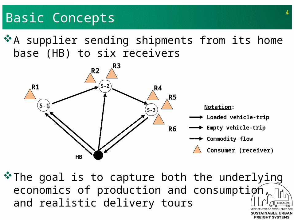
A supplier sending shipments from its home base (HB) to six receivers

The goal is to capture both the underlying economics of production and consumption, and realistic delivery tours

4

HB

S-2

Loaded vehicle-trip

Commodity flow

Notation:

Consumer (receiver)

Empty vehicle-trip

S-1S-3

R1

 

R2 

R3

 

 

 

R5

R6

R4

 

Empirical Evidence onUrban Freight Tours

5

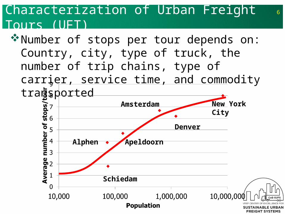
Characterization of Urban Freight Tours (UFT)Number of stops per tour depends on:

Country, city, type of truck, the number of trip chains, type of carrier, service time, and commodity transported

6

Schiedam

Alphen Apeldoorn

Amsterdam

Denver

New York City

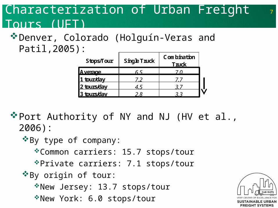
Characterization of Urban Freight Tours (UFT)Denver, Colorado (Holguín-Veras and

Patil,2005):

Port Authority of NY and NJ (HV et al., 2006):By type of company:

Common carriers: 15.7 stops/tour Private carriers: 7.1 stops/tour

By origin of tour:New Jersey: 13.7 stops/tour New York: 6.0 stops/tour

7

Stops/Tour Single TruckCombination

TruckAverage 6.5 7.01 tour/day 7.2 7.72 tours/day 4.5 3.73 tours/day 2.8 3.3

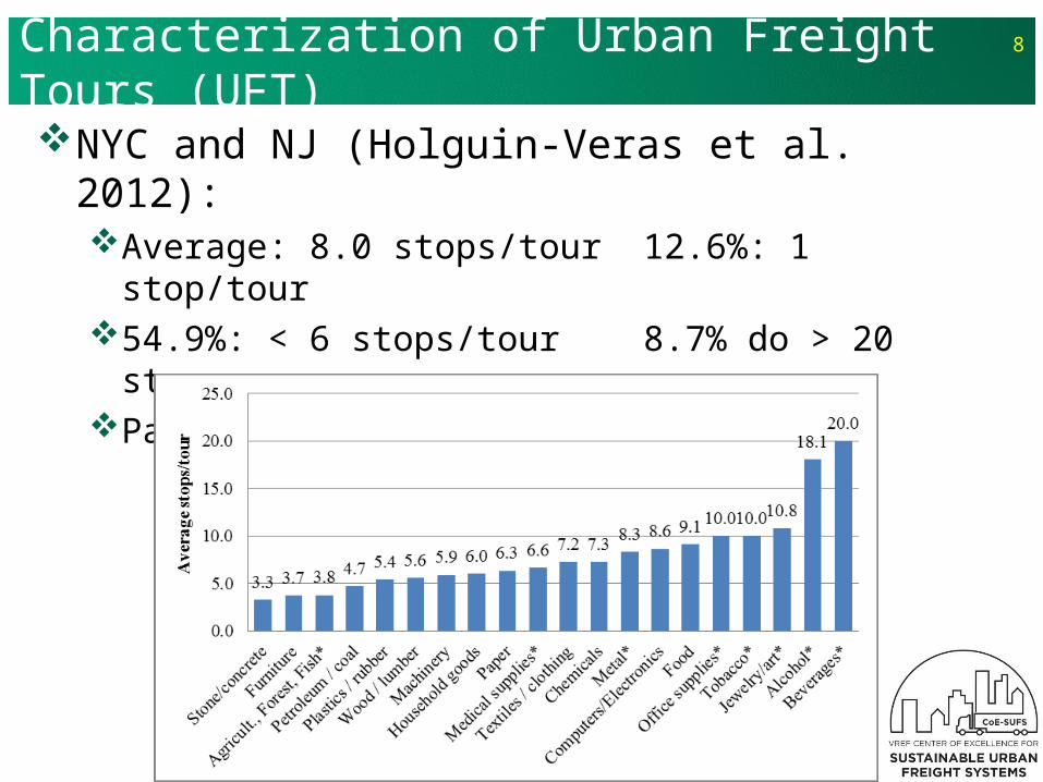
Characterization of Urban Freight Tours (UFT)NYC and NJ (Holguin-Veras et al. 2012):

Average: 8.0 stops/tour 12.6%: 1 stop/tour 54.9%: < 6 stops/tour 8.7% do > 20 stopsParcel deliveries: 50-100 stops/tour

8

Urban Freight Tour Models

9

Urban Freight Tour Models

The UFT models could be subdivided into:Simulation modelsHybrid modelsAnalytical models

10

Simulation Models

11

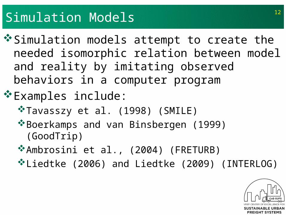
Simulation Models

Simulation models attempt to create the needed isomorphic relation between model and reality by imitating observed behaviors in a computer program

Examples include: Tavasszy et al. (1998) (SMILE)Boerkamps and van Binsbergen (1999) (GoodTrip)Ambrosini et al., (2004) (FRETURB)Liedtke (2006) and Liedtke (2009) (INTERLOG)

12

Hybrid Models

13

Hybrid Models

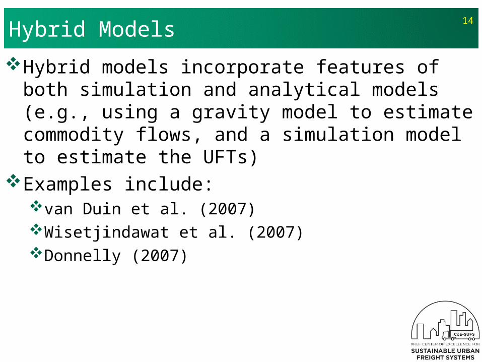
Hybrid models incorporate features of both simulation and analytical models (e.g., using a gravity model to estimate commodity flows, and a simulation model to estimate the UFTs)

Examples include: van Duin et al. (2007) Wisetjindawat et al. (2007) Donnelly (2007)

14

Analytical Models

15

Analytical Models

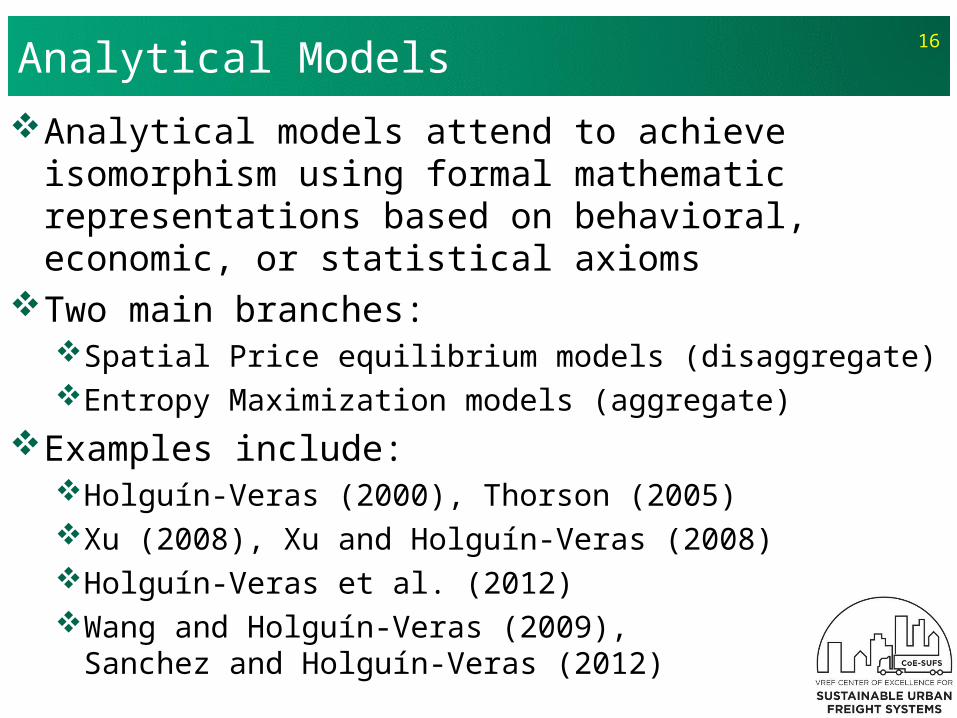
Analytical models attend to achieve isomorphism using formal mathematic representations based on behavioral, economic, or statistical axioms

Two main branches:Spatial Price equilibrium models (disaggregate)Entropy Maximization models (aggregate)

Examples include: Holguín-Veras (2000), Thorson (2005)Xu (2008), Xu and Holguín-Veras (2008)Holguín-Veras et al. (2012)Wang and Holguín-Veras (2009),

Sanchez and Holguín-Veras (2012)

16

Entropy Maximization Tour Flow Model

17

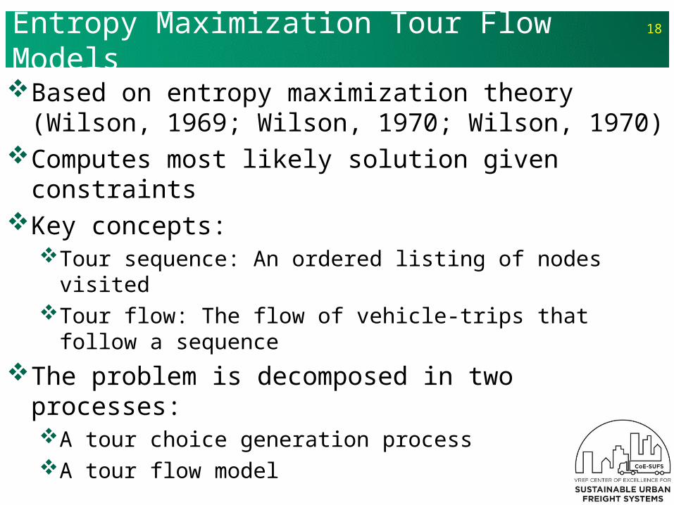
Entropy Maximization Tour Flow Models

Based on entropy maximization theory (Wilson, 1969; Wilson, 1970; Wilson, 1970)

Computes most likely solution given constraintsKey concepts:

Tour sequence: An ordered listing of nodes visitedTour flow: The flow of vehicle-trips that follow a

sequence

The problem is decomposed in two processes: A tour choice generation processA tour flow model

18

Entropy Maximization Tour Flow Model

Tour choice: To estimate sensible node sequences Tour flow: To estimate the number of trips traveling

along a particular node sequence

23/4/18

19

Tour choice generation Tour flows

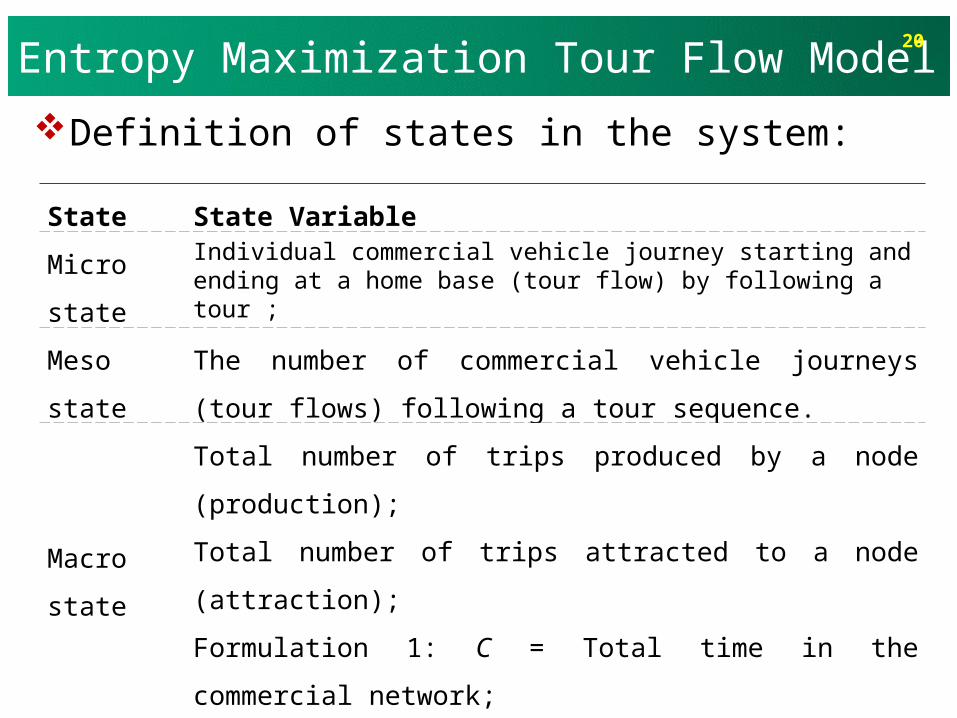
Entropy Maximization Tour Flow Model20

Definition of states in the system:

State State Variable

Micro stateIndividual commercial vehicle journey starting and ending at a home base (tour flow) by following a tour ;

Meso stateThe number of commercial vehicle journeys (tour flows) following

a tour sequence.

Macro stateTotal number of trips produced by a node (production);

Total number of trips attracted to a node (attraction);

Formulation 1: C = Total time in the commercial network;

Formulation 2: CT = Total travel time in the commercial network;

CH = Total handling time in the commercial

network.

Static version of EM Tour Flow Model

21

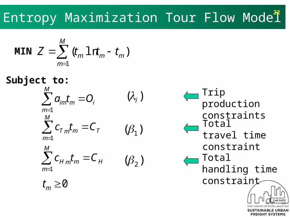
The equivalent model of formulation 2:Entropy Maximization Tour Flow Model

Trip production constraints

Total travel time constraint

Total handling time constraint

22

M

mmmm tttZ

1

)ln(

i

M

mmim Ota

1

T

M

mmmT Ctc

1

H

M

mmmH Ctc

1

0mt

)( i

)( 1

)( 2

MIN

Subject to:

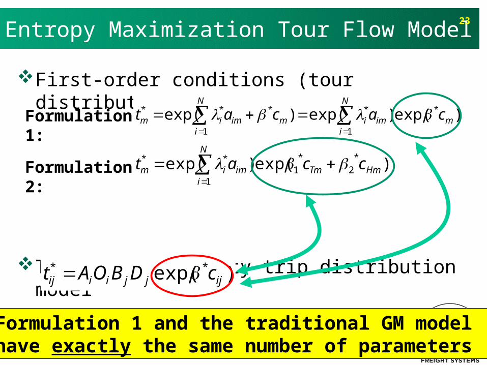
First-order conditions (tour distribution models)

Traditional gravity trip distribution model

Entropy Maximization Tour Flow Model

)exp()exp()exp( *

1

*

1

***m

N

iimi

N

imimim cacat

23

)exp( **ijjjiiij cDBOAt

)exp()exp( *2

*1

1

**HmTm

N

iimim ccat

Formulation 1:

Formulation 2:

Formulation 1 and the traditional GM model have exactly the same number of parameters

Entropy Maximization Tour Flow Model

The optimal tour flows are found under the objective of maximizing the entropy for the system

The tour flows are a function of tour impedance and Lagrange multipliers associated with the trip productions and attractions along that tour

Successfully tested with Denver, Colorado, data:The MAPE of the estimated tour flows is less than

6.7% given the observed tours are usedMuch better than the traditional GM

24

25Case Study: Denver Metropolitan Area

Test network919 TAZs among which 182 TAZs contain home

bases of commercial vehicles613 tours, representing a total of 65,385 tour flows /

day Calibration done with 17,000 tours (from heuristics)

Estimation procedureSorting input data: aggregate the observed tour

flows to obtain trip productions and total impedanceEstimation: estimate the tour flows distributed on

these tours using the entropy maximization formulations

Assessing performance: compare the estimated tour flows with the observed tour flows

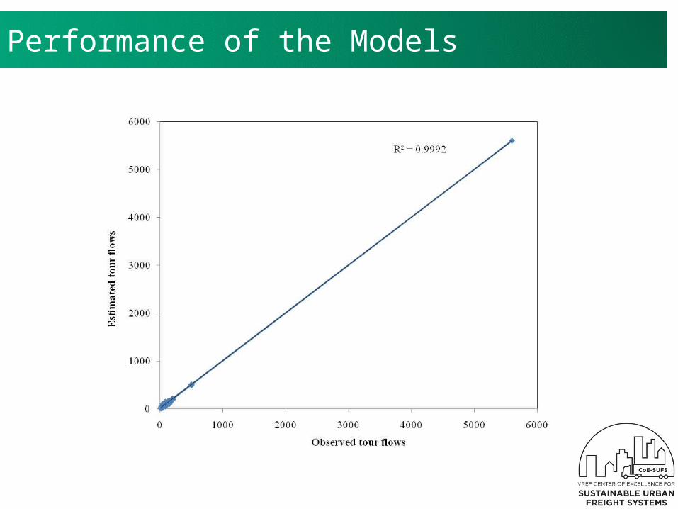
Estimated vs. observed tour flowsPerformance of the Models

Time-Dependent Freight Tour Synthesis Model

27

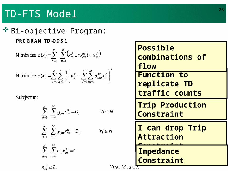
TD-FTS Model

Bi-objective Program:

28

PROGRAM TD-ODS 1

Minimize

M

m

dm

dm

dm

K

d

xxxxz11

)ln()( (1)

Minimize 2

1 1

'

1 12

1)(

A

a

K

k

K

d

M

m

dm

kdam

ka xvxe (2)

Subject to:

M

mi

dmim

K

d

NiOxg11

(3)

M

mj

dmjm

K

d

NjDx11

(4)

M

m

dmm

K

d

Cxc11

(5)

KdMmx dm ,,0

(6)

Function to replicate TD traffic counts

Trip Production Constraint

I can drop Trip Attraction ConstraintImpedance Constraint

Possible combinations of flow

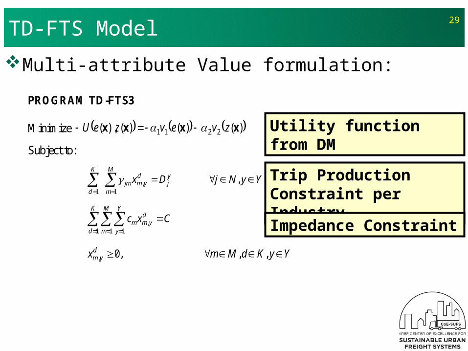
TD-FTS Model

Multi-attribute Value formulation:

29

PROGRAM TD-FTS3

Minimize )()()(),( 2211 xxxx zvevzeU

Subject to:

M

m

yj

dymjm

K

d

YyNjDx1

,1

,

)( , yj

K

d

M

m

Y

y

dymm Cxc

1 1 1,

)(

YyKdMmxdym ,,,0,

Trip Production Constraint per IndustryImpedance Constraint

Utility function from DM

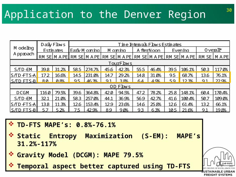
Application to the Denver Region30

RMSE MAPE RMSE MAPE RMSE MAPE RMSE MAPE RMSE MAPE RMSE MAPE

S/TD-EM 39.8 31.2% 58.5 274.7% 45.6 42.3% 55.5 46.4% 39.5 106.1% 50.3 117.0%S/TD-FTS-A 17.2 16.6% 14.5 231.0% 14.7 29.2% 14.8 31.0% 9.5 68.7% 13.6 76.1%S/TD FTS-B 8.0 0.8% 9.5 46.3% 9.1 3.8% 6.4 4.9% 5.9 12.3% 9.1 22.9%

DCGM 116.0 79.5% 39.6 364.8% 42.0 94.5% 47.2 78.2% 25.8 148.1% 60.4 170.4%S/TD-EM 32.1 21.0% 58.3 257.0% 44.1 36.9% 56.9 42.7% 41.6 100.4% 50.7 109.0%

S/TD-FTS-A 13.8 11.3% 12.6 153.4% 12.9 23.6% 14.6 25.8% 12.6 61.4% 13.2 66.1%S/TD FTS-B 5.7 5.2% 7.5 42.9% 8.9 9.0% 9.3 6.3% 10.5 21.6% 9.1 19.8%

Tour Flows

OD Flows

Modeling Approach

Daily Flows Estimates

Time Intervals Flows EstimatesEarly Morning Morning After Noon Evening Overall*

TD-FTS MAPE’s: 0.8%-76.1%

Static Entropy Maximization (S-EM): MAPE’s 31.2%-117%

Gravity Model (DCGM): MAPE 79.5%

Temporal aspect better captured using TD-FTS

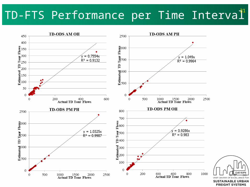
TD-FTS Performance per Time Interval31

Multiclass Equilibrium Demand Synthesis

32

Multiclass: two or more classes of travelers with different behavioral or choice characteristics

Vehicle classes are related under the same objective function

Multiclass equilibrium demand synthesis (MEDS)

Multiclass traffic33

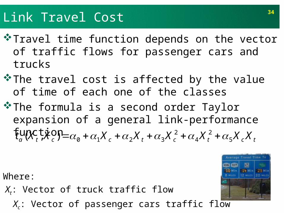
Travel time function depends on the vector of traffic flows for passenger cars and trucks

The travel cost is affected by the value of time of each one of the classes

The formula is a second order Taylor expansion of a general link-performance function

 

Where: Xt: Vector of truck traffic flow

Xc: Vector of passenger cars traffic flow

Link Travel Cost34

tctctccta XXXXXXXXt 52

42

3210),(

In a multiclass equilibrium, the cost functions of the modes are asymmetric, traffic flows interact

The user optimal assignment cannot be written as an optimization problem

The User Equilibrium (UE) problem could be addressed using a Variational Inequality (VI) Problem

Multiclass Equilibrium35

0)(),()(),( ****** ij

ijijT

ijmijm

mmT

ijmm TTTtCttttC00 * mmm tCC

00 * ijijij TCC

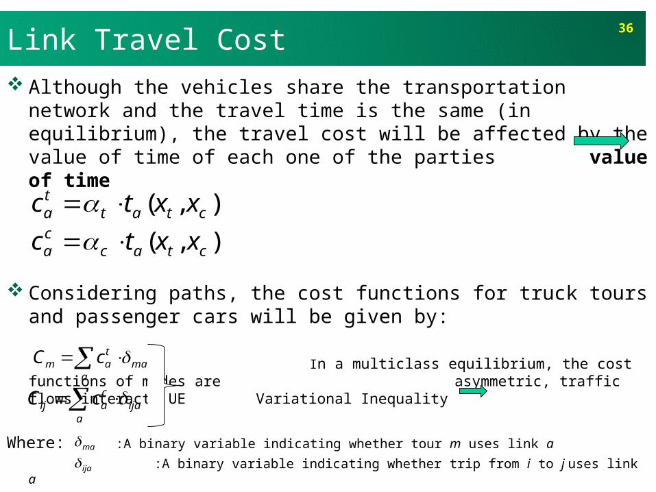
Although the vehicles share the transportation network and the travel time is the same (in equilibrium), the travel cost will be affected by the value of time of each one of the parties value of time

Considering paths, the cost functions for truck tours and passenger cars will be given by:

In a multiclass equilibrium, the cost functions of modes are asymmetric, traffic flows interact. UE Variational Inequality

Where: :A binary variable indicating whether tour m uses link a

:A binary variable indicating whether trip from i to j uses link a

Link Travel Cost36

),( ctatta xxtc

),( ctacca xxtc

a

matam cC

ijaa

caij cC

ma

ija

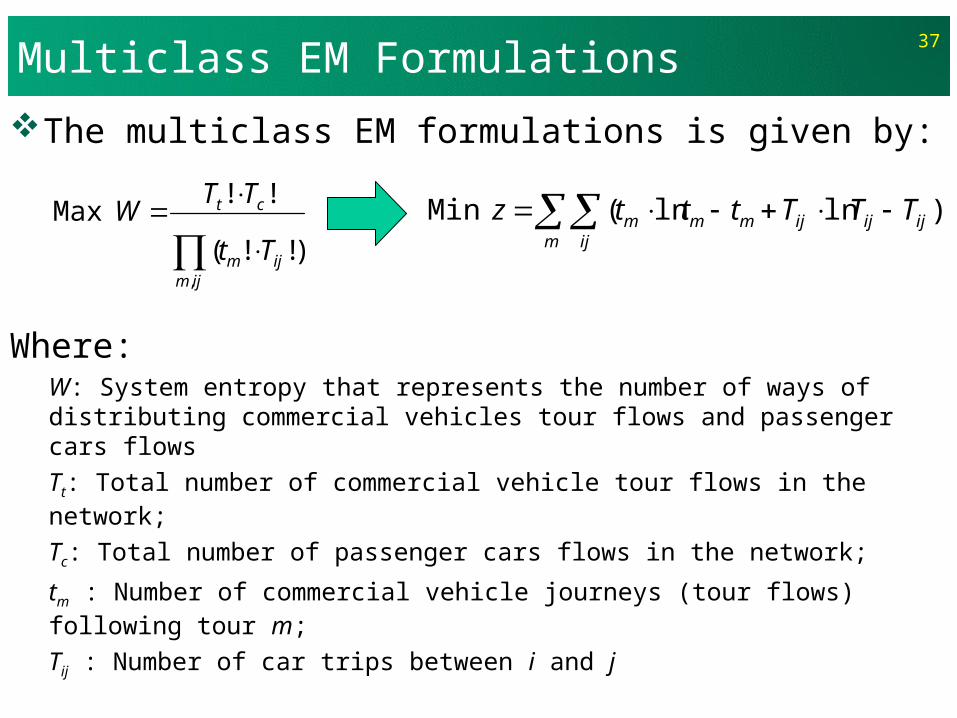
Multiclass EM Formulations

The multiclass EM formulations is given by:

Where:W: System entropy that represents the number of ways of distributing commercial vehicles tour flows and passenger cars flowsTt: Total number of commercial vehicle tour flows in the network;

Tc: Total number of passenger cars flows in the network;

tm : Number of commercial vehicle journeys (tour flows) following tour m;Tij : Number of car trips between i and j

37

ijmijm

ct

Tt

TTW

,

)! !(

! !Max

m ijijijijmmm TTTtttz )ln ln(Min

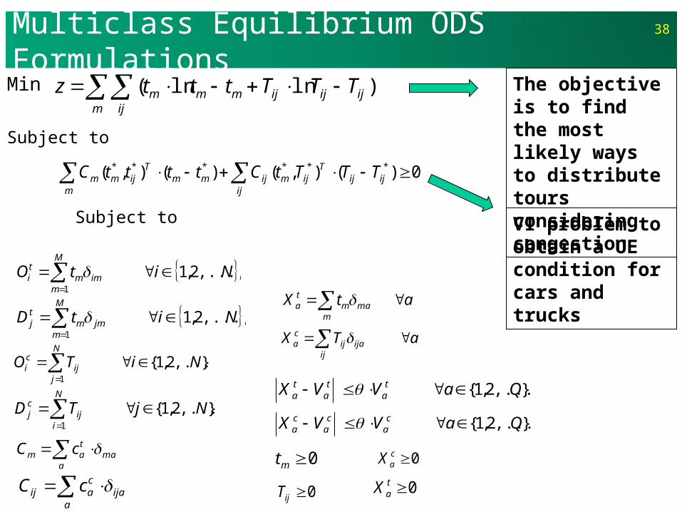
Multiclass Equilibrium ODS FormulationsMin

Subject to

Subject to

38

m ij

ijijijmmm TTTtttz )ln ln(

0)(),()(),( ****** ij

ijijT

ijmijm

mmT

ijmm TTTtCttttC

NitOM

mimm

ti ,...,2,1

1

NitDM

mjmm

tj ,...,2,1

1

},...2,1{ 1

NiTON

jij

ci

},...2,1{ 1

NjTDN

iij

cj

a

matam cC

ijaa

caij cC

atXm

mamta

aTXij

ijaijca

},...2,1{ QaVVX ta

ta

ta

},...2,1{ QaVVX ca

ca

ca

0mt

0ijT 0 taX

0 caX

VI problem to obtain a UE condition for cars and trucks

The objective is to find the most likely ways to distribute tours considering congestion

Spatial Price Equilibrium Tour Models

39

General principles

The models estimate commodity flows and vehicle trips that arise under competitive market equilibrium

Conceptual advantages:Account for toursProvide a coherent framework to jointly model the

joint formation of commodity flows and vehicle trips

Based on the seminal work of Samuelson (1952), as it seeks to maximize the economic welfare associated with the consumption and transportation of the cargo, taking into account the formation of UFTs

40

Two flavors

Independent Shipper-Carrier Operations:Carrier and Shipper are independent companiesCarrier travels empty from its base to pick up cargo

at shipper’s location(s)Carrier delivers cargo to shipper’s customersCarrier travels empty back to its base

Integrated Shipper-Carrier Operations:Carrier and Shipper are part of the same companyCarrier is loaded at shipper’s location(s)Carrier delivers cargo to shipper’s customersCarrier travels empty back to its base

41

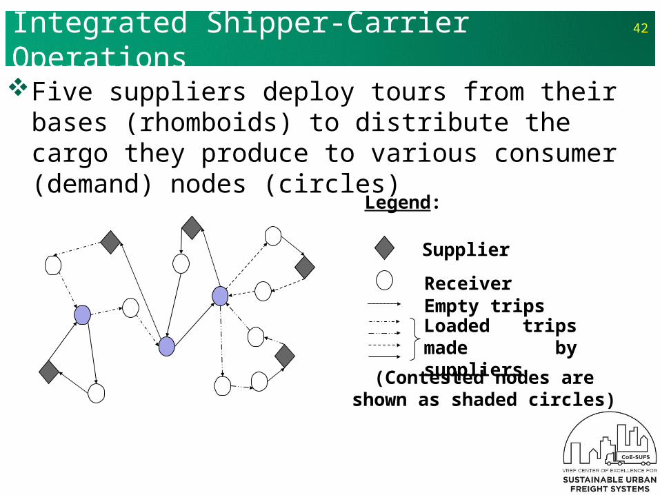
Integrated Shipper-Carrier Operations

Five suppliers deploy tours from their bases (rhomboids) to distribute the cargo they produce to various consumer (demand) nodes (circles)

42

Legend:

(Contested nodes are shown as shaded circles)

Loaded trips made by suppliers

Empty tripsReceiver

Supplier

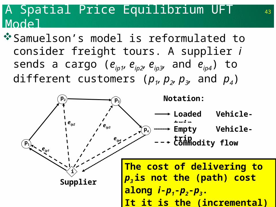
A Spatial Price Equilibrium UFT Model

Samuelson’s model is reformulated to consider freight tours. A supplier i sends a cargo (eip1, eip2, eip3, and eip4) to different customers (p1, p2, p3, and p4)

43

Supplier

p1

p2 p3

p4

i

eip1

eip3

eip2

eip4 Commodity flow

Notation:

Loaded Vehicle-trip

Empty Vehicle-trip

The cost of delivering to p3 is not the (path) cost along i-p1-p2-p3. It it is the (incremental) cost from p2 to p3, plus part of the empty trip cost.

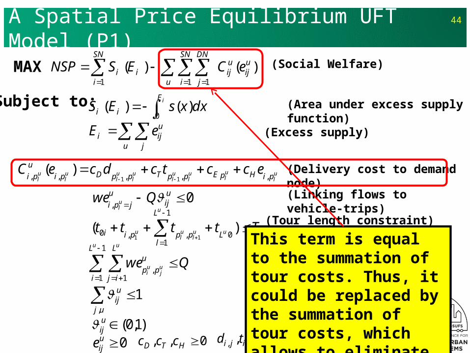
A Spatial Price Equilibrium UFT Model (P1)44

iE

ii dxxsES0

)()(

u j

uiji eE

0,

uij

u

jpiQwe u

l

Ttttt u

u

ul

ul

u L

L

lpppii

)(0

1

1,,0

11

Qwe

u u

uj

ui

L

i

L

ij

u

pp

1

1 1,

1,

uj

uij

)1,0(uij

0uije 0,, HTD ccc 0, ,, jiji td

(Social Welfare)

(Area under excess supply function)

(Excess supply)

(Linking flows to vehicle-trips)

(Tour length constraint)

(Capacity constraint)

(Conservation of flow)

(Integrality)

(Non-negativity)

u

SN

i

uij

uij

DN

ji

SN

ii eCESNSP

1 11

)()(

ul

ul

ul

ul

ul

ul

ul

ul piHpEppTppDpi

u

piecctcdceC

,,,,, 11)(

(Delivery cost to demand node)

MAX

Subject to:

This term is equal to the summation of tour costs. Thus, it could be replaced by the summation of tour costs, which allows to eliminate the delivery cost constraint

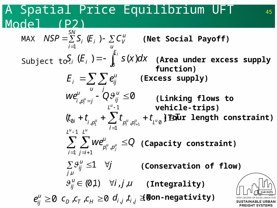
A Spatial Price Equilibrium UFT Model (P2)

MAX

Subject to:

45

u

uVi

SN

ii CESNSP )(

1

iE

ii dxxsES0

)()(

u j

uiji eE

0,

uij

u

jpiQwe u

l

Ttttt u

u

ul

ul

u L

L

lpppii

)(0

1

1,,0

11

Qwe

u u

uj

ui

L

i

L

ij

u

pp

1

1 1,

juj

uij 1

,

ujiuij ,,)1,0(

0uije 0,, HTD ccc 0, ,, jiji td

(Net Social Payoff)

(Area under excess supply function)

(Excess supply)

(Linking flows to vehicle-trips)

(Tour length constraint)

(Capacity constraint)

(Conservation of flow)

(Integrality)

(Non-negativity)

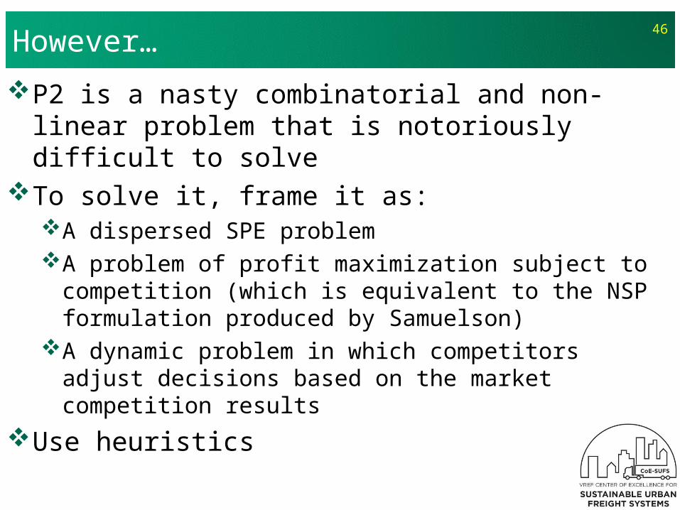
However…

P2 is a nasty combinatorial and non-linear problem that is notoriously difficult to solve

To solve it, frame it as:A dispersed SPE problemA problem of profit maximization subject to

competition (which is equivalent to the NSP formulation produced by Samuelson)

A dynamic problem in which competitors adjust decisions based on the market competition results

Use heuristics

46

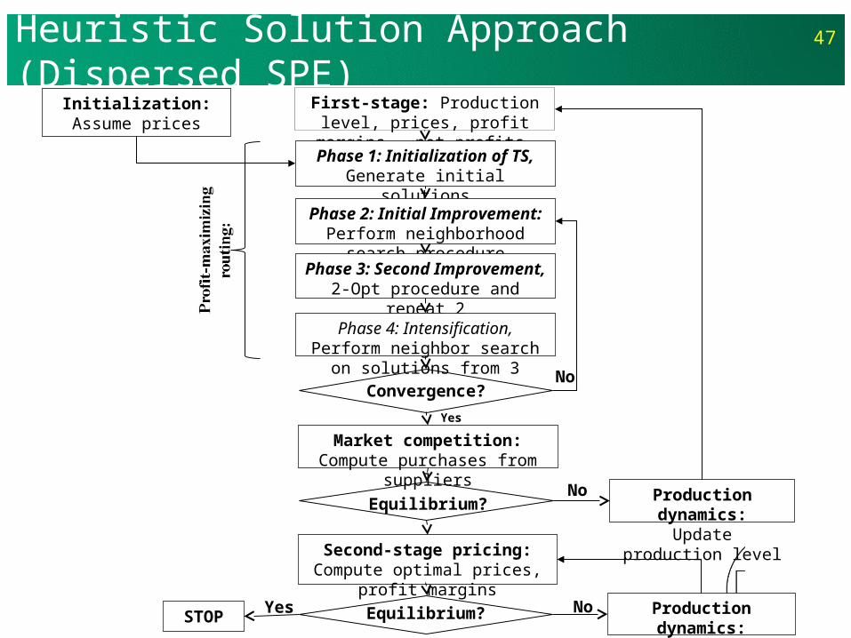
Heuristic Solution Approach (Dispersed SPE)

47

First-stage: Production level, prices, profit margins, net profits

Second-stage pricing: Compute optimal prices, profit margins

Phase 1: Initialization of TS, Generate initial solutions

Phase 2: Initial Improvement: Perform neighborhood search

procedure

 Phase 3: Second Improvement, 2-

Opt procedure and repeat 2

Phase 4: Intensification, Perform neighbor search on solutions from 3

 

Equilibrium?Production dynamics:Update production level

Initialization: Assume prices

 Convergence?No

Market competition: Compute purchases from suppliers

  No

Yes

STOP  Equilibrium? Production dynamics:Update production level

NoYes

Equilibrium Results48

0

20

40

60

80

100

0 20 40 60 80 100

Y (m

iles)

X (miles)

Consumers

SuppliersC2, D=8

C4, D=10

C3, D=4

C1, D=6

S1

S2

0

20

40

60

80

100

0 20 40 60 80 100

Y (m

iles)

X (miles)

Consumers

SuppliersC2, D=8

C4, D=10

C3, D=4

C1, D=6

S1

S2

)(

)()1(

)1(

12

,,

iij

hujITijuhtQijuht

ijtop

iijt ssD

mmP

sP

0

20

40

60

80

100

0 20 40 60 80 100

Y (m

iles)

X (miles)

Consumers

SuppliersC2, D=8

C4, D=10

C3, D=4

C1, D=6

S1

S2

C4

(2.2

4, .7

3)

(2.84, .89)

C4

(1.61, .47)

(6.41, .10)

(3.76, .10)

(5.16, .10)

(2.39, .10)

(3.59, .97)

Two suppliers, four customers Vehicle-tours

Commodity flows and prices

Concluding Remarks

49

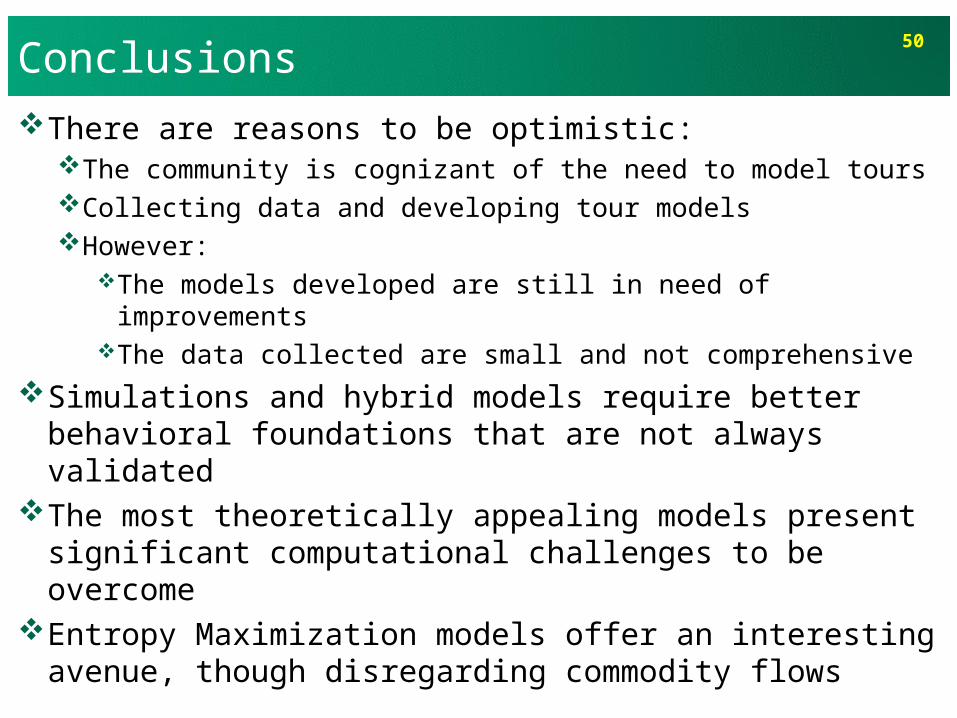
Conclusions

There are reasons to be optimistic:The community is cognizant of the need to model toursCollecting data and developing tour modelsHowever:

The models developed are still in need of improvementsThe data collected are small and not comprehensive

Simulations and hybrid models require better behavioral foundations that are not always validated

The most theoretically appealing models present significant computational challenges to be overcome

Entropy Maximization models offer an interesting avenue, though disregarding commodity flows

50

References

51

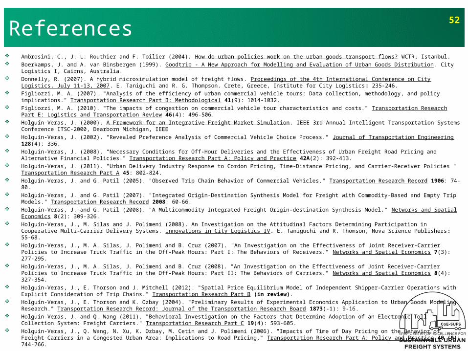
References Ambrosini, C., J. L. Routhier and F. Toilier (2004). How do urban policies work on the urban goods transport flows? WCTR, Istanbul. Boerkamps, J. and A. van Binsbergen (1999). Goodtrip - A New Approach for Modelling and Evaluation of Urban Goods Distribution. City Logistics I,

Cairns, Australia. Donnelly, R. (2007). A hybrid microsimulation model of freight flows. Proceedings of the 4th International Conference on City Logistics, July 11-13,

2007. E. Taniguchi and R. G. Thompson. Crete, Greece, Institute for City Logistics: 235-246. Figliozzi, M. A. (2007). "Analysis of the efficiency of urban commercial vehicle tours: Data collection, methodology, and policy implications."

Transportation Research Part B: Methodological 41(9): 1014-1032. Figliozzi, M. A. (2010). "The impacts of congestion on commercial vehicle tour characteristics and costs." Transportation Research Part E: Logistics

and Transportation Review 46(4): 496-506. Holguín-Veras, J. (2000). A Framework for an Integrative Freight Market Simulation. IEEE 3rd Annual Intelligent Transportation Systems Conference

ITSC-2000, Dearborn Michigan, IEEE Holguín-Veras, J. (2002). "Revealed Preference Analysis of Commercial Vehicle Choice Process." Journal of Transportation Engineering 128(4): 336. Holguín-Veras, J. (2008). "Necessary Conditions for Off-Hour Deliveries and the Effectiveness of Urban Freight Road Pricing and Alternative Financial

Policies." Transportation Research Part A: Policy and Practice 42A(2): 392-413. Holguín-Veras, J. (2011). "Urban Delivery Industry Response to Cordon Pricing, Time-Distance Pricing, and Carrier-Receiver Policies " Transportation

Research Part A 45: 802-824. Holguín-Veras, J. and G. Patil (2005). "Observed Trip Chain Behavior of Commercial Vehicles." Transportation Research Record 1906: 74-80. Holguín-Veras, J. and G. Patil (2007). "Integrated Origin-Destination Synthesis Model for Freight with Commodity-Based and Empty Trip Models."

Transportation Research Record 2008: 60-66. Holguín-Veras, J. and G. Patil (2008). "A Multicommodity Integrated Freight Origin–destination Synthesis Model." Networks and Spatial Economics

8(2): 309-326. Holguín-Veras, J., M. Silas and J. Polimeni (2008). An Investigation on the Attitudinal Factors Determining Participation in Cooperative Multi-Carrier

Delivery Systems. Innovations in City Logistics IV. E. Taniguchi and R. Thomson, Nova Science Publishers: 55-68. Holguín-Veras, J., M. A. Silas, J. Polimeni and B. Cruz (2007). "An Investigation on the Effectiveness of Joint Receiver-Carrier Policies to Increase Truck

Traffic in the Off-Peak Hours: Part I: The Behaviors of Receivers." Networks and Spatial Economics 7(3): 277-295. Holguín-Veras, J., M. A. Silas, J. Polimeni and B. Cruz (2008). "An Investigation on the Effectiveness of Joint Receiver-Carrier Policies to Increase Truck

Traffic in the Off-Peak Hours: Part II: The Behaviors of Carriers." Networks and Spatial Economics 8(4): 327-354. Holguín-Veras, J., E. Thorson and J. Mitchell (2012). "Spatial Price Equilibrium Model of Independent Shipper-Carrier Operations with Explicit

Consideration of Trip Chains." Transportation Research Part B (in review). Holguín-Veras, J., E. Thorson and K. Ozbay (2004). "Preliminary Results of Experimental Economics Application to Urban Goods Modeling Research."

Transportation Research Record: Journal of the Transportation Research Board 1873(-1): 9-16. Holguín-Veras, J. and Q. Wang (2011). "Behavioral Investigation on the Factors that Determine Adoption of an Electronic Toll Collection System:

Freight Carriers." Transportation Research Part C 19(4): 593-605. Holguín-Veras, J., Q. Wang, N. Xu, K. Ozbay, M. Cetin and J. Polimeni (2006). "Impacts of Time of Day Pricing on the Behavior of Freight Carriers in a

Congested Urban Area: Implications to Road Pricing." Transportation Research Part A: Policy and Practice 40 (9): 744-766.

52

References Holguín-Veras, J., N. Xu and J. Mitchell (2012). "A Dynamic Spatial Price Equilibrium Model of Integrated Production-Transportation

Operations Considering Freight Tours." (in review). Hunt, J. D. and K. J. Stefan (2007). "Tour-based microsimulation of urban commercial movements." Transportation Research Part B:

Methodological 41(9): 981-1013. Liedtke, G. (2006). An actor-based approach to commodity transport modelling. Ph.D., Karlsruhe Universitat. Liedtke, G. (2009). "Principles of micro-behavior commodity transport modeling." Transportation Research Part E: Logistics and

Transportation Review 45(5): 795-809. McFadden, D., C. Winston and A. Boersch-Supan (1986). Joint Estimation of Freight Transportation Decisions Under Non-Random

Sampling. Discussion Paper, Harvard University. Ruan, M., J. Lin and K. Kawamura (2012). "Modeling urban commercial vehicle daily tour chaining." Transportation Research Part E:

Logistics and Transportation Review 48(6): 1169-1184. Samuelson, P. A. (1952). "Spatial Price Equilibrium and Linear Programming." American Economic Review 42(3): 283-303. Samuelson, R. D. (1977). Modeling the Freight Rate Structure. Cambridge MA, Center for Transportation Studies, Massachusetts

Institute of Technology. Stefan, K., J. McMillan and J. Hunt (2005). "Urban Commercial Vehicle Movement Model for Calgary, Alberta, Canada." Transportation

Research Record: Journal of the Transportation Research Board 1921: 1-10. Tavasszy, L. A., B. Smeenk and C. J. Ruijgrok (1998). "A DSS for Modelling Logistics Chains in Freight Transport Systems Analysis."

International Transactions in Operational Research 5(6): 447-459. Thorson, E. (2005). The Integrative Freight Market Simulation: An Application of Experimental Economics and Algorithmic Solutions.

Ph.D., Rensselaer Polytechnic Institute. van Duin, J. H. R., L. A. Tavasszy and E. Taniguchi (2007). "Real time simulation of auctioning and re-scheduling processes in hybrid

freight markets." Transportation Research Part B: Methodological 41(9): 1050-1066. Vleugel, J. and M. Janic (2004). Route choice and the impact of ‘logistic routes’. Logistics Systems for Sustainable Cities. E. Taniguchi

and R. Thompson, Elsevier. Wang, Q. (2008). Tour Based Urban Freight Travel Demand Models. PhD, Rensselaer Polytechnic Institute. Wang, Q. and J. Holguín-Veras (2008). "Investigation of Attributes Determining Trip Chaining Behavior in Hybrid Microsimulation Urban

Freight Models." Transportation Research Record: Journal of the Transportation Research Board 2066: 1-8. Wang, Q. and J. Holguín-Veras (2009). Tour-based Entropy Maximization Formulations of Urban Commercial Vehicle Movements. 2009

Annual Meeting of the Transportation Research Board. CDROM. Wilson, A. G. (1969). "The use of entropy maximising models in the theory of trip distribution, mode split " Journal of Transport

Economics and Policy 108-126. Wilson, A. G. (1970). Entropy in Urban and Regional Modelling. London, Pion. Wilson, A. G. (1970). "The use of the concept of entropy in system modelling." Operational Research Quarterly 21(2): 247-265. Wisetjindawat, W., K. Sano, S. Matsumoto and P. Raothanachonkun (2007). Micro-Simulation Model for Modeling Freight Agents

Interactions in Urban Freight Movement. 86th Annual Meeting of the Transportation Research Board

53

Thanks! Questions?

54