S

Ea

b

c

a

ARRAA

KCMTU

1

ofteolsuiclqsia

(

h1

Urban Forestry & Urban Greening 17 (2016) 104–115

Contents lists available at ScienceDirect

Urban Forestry & Urban Greening

j ourna l h om epage: www.elsev ier .com/ locate /u fug

tructure, function and value of street trees in California, USA

. Gregory McPherson a,∗, Natalie van Doorn b, John de Goede c

USDA Forest Service, Pacific Southwest Research Station, 1731 Research Park Dr., Davis, CA 95618, USAUSDA Forest Service, Pacific Southwest Research Station, 800 Buchanan St. Albany, CA 94710, USAUniversity of California Davis, Information Center for the Environment, Davis, CA 95616, USA

r t i c l e i n f o

rticle history:eceived 9 December 2015eceived in revised form 22 March 2016ccepted 30 March 2016vailable online 16 April 2016

eywords:ommunity forestunicipal forest

ree benefitsrban ecosystem services

a b s t r a c t

This study compiled recent inventory data from 929,823 street trees in 50 cities to determine trends intree number and density, identify priority investments and create baseline data against which the effi-cacy of future practices can be evaluated. The number of street trees increased from 5.9 million in 1988to 9.1 million in 2014, about one for every four residents. Street tree density declined from 65.6 to 46.6trees per km, nearly a 30% drop. City streets are at 36.3% of full stocking. State-wide, only London plane-tree (Platanus × hispanica) comprises over 10% of the total, suggesting good state-wide species diversity.However, at the city scale, 39 communities were overly reliant on a single species. The state’s street treesremove 567,748 t CO2 (92,253 t se) annually, equivalent to taking 120,000 cars off the road. Their assetvalue is $2.49 billion ($75.1 million se). The annual value (USD) of all ecosystem services is $1.0 billion($58.3 million se), or $110.63 per tree ($29.17 per capita). Given an average annual per tree management

cost of $19.00, $5.82 in benefit is returned for every $1 spent. Management implications could includeestablishing an aggressive program to plant the 16 million vacant sites and replace removed trees, whilerestricting planting of overabundant species. Given the tree population’s youth there is likely need toinvest in pruning young trees for structure and form, which can reduce subsequent costs for treatingdefects in mature trees.

Published by Elsevier GmbH.

. Introduction

Street trees, defined as trees growing along public street right-f-way and managed by the city, account for a relatively smallraction of the entire urban forest, but are prominent because ofheir visual and physical impacts on the quality of urban life. Forxample, although street trees in the City of Chicago accounted fornly 10% of the city’s tree population, they comprised 24% of total

eaf surface area (McPherson et al., 1997). This study examines thetructure, function and value of California’s current street tree pop-lation. Several studies indicate that street tree density in California

s declining. One goal of this study is to determine if this remainsause for concern. A second goal is to prioritize management chal-enges at the state and regional levels. For the first time, this studyuantifies the value of ecosystem services produced by California’s

treet tree population. This assessment provides a baseline for Cal-fornia and it is among the first to present a comprehensive view of

state’s street tree resource.

∗ Corresponding author.E-mail addresses: gmcpherson@fs.fed.us (E.G. McPherson), nvandoorn@fs.fed.us

N. van Doorn), jmdegoede@ucdavis.edu (J. de Goede).

ttp://dx.doi.org/10.1016/j.ufug.2016.03.013618-8667/Published by Elsevier GmbH.

Municipal forests consist of street and park trees managed forthe public good. Street tree populations have their own uniquestructure, tending to be less diverse, containing more large-staturespecies and exhibiting higher levels of spatial continuity than othercomponents of the urban forest (Jim and Liu, 2001).

The following review begins with a description of street treeassessments conducted at large scale, for the entire United Statesand for several states within the U.S. It then narrows its focus tostudies concerned with municipal forests in the state of California.

1.1. United States and state-wide assessments

In 1989, an assessment of street trees in 320 U.S. cities wasconducted (Kielbaso and Cotrone, 1990). There were identifiedapproximately 61.6 million street trees averaging 63.4 trees perstreet km (102/mile) and 0.4 per person. Assuming trees wereplanted 15.2 m (50 ft) apart, there was room for planting another66 million street trees. The ratio of trees planted to removed each

year was 0.99, a decrease from 1.2 found several years earlier. Theauthors reported that this ratio dropped in larger cities, as did thecondition rating of trees. The asset value of the nation’s street treeswas an estimated $30 billion, assuming $500 per tree.

ry & U

(pad

amf2p(emsitCK(sap2

in1s

t(i(tc3i1cDtt

dmsfdewsgc(

1

mitae(s

E.G. McPherson et al. / Urban Forest

A more recent U.S. survey focused on public tree managementTschantz and Sacamano, 1994). In 1994, the average number ofublically-owned street and park trees was 0.63 per capita. Theverage municipal tree management budget was $2.49 per capita,own from $4.14 in 1986.

State-wide assessments in the U.S. have varied in their methodsnd scope. A 1994 survey of public trees in 20 Michigan com-unities estimated 1.67 million street trees state-wide with 49%

ull stocking (Wildenthal and Keilbaso, 1994). Between 2001 and003 the US Forest Service Forest Health Monitoring (FHM) teamartnered with Urban & Community Forestry staff in WisconsinCumming et al., 2008), Maryland and Massachusetts (Cummingt al., 2006) to survey street trees state-wide. The most seriousanagement issue noted was lack of species diversity. The top five

pecies accounted for 45% to 60% of the total street tree populations,ndicating overreliance on a small number of species. The suscep-ibility of black walnut (Juglans nigra) street trees to Thousandsankers Disease (resulting from the fungus Geosmithia morbida) inansas (Treiman et al., 2010) and ash trees to emerald ash borer

Agrilus planipennis) in South Dakota (Ball et al., 2007) were theubjects of state-wide analyses of tree inventories. A region-wide-ssessment used street tree inventory data to examine threatsosed by exotic borers in eastern North America (Raupp et al.,006).

A 2008 study of street trees in 23 Indiana communities applied-Tree Streets (formerly STRATUM) software to calculate the eco-omic value of ecosystem services produced annually by the state’s.42 million street trees (Davey Resource Group, 2010a,b). Annualervices were valued at $78.7 million or $55.51 per tree.

In 2010 street trees on 284 plots in 44 Missouri communi-ies were resurveyed after previous inventories in 1989 and 1999Treiman et al., 2011a,b). This 20-year longitudinal assessments unique. Street tree density increased from 28.7 trees per km46.2/mile) in 1989 to 40 (64.3/mi) in 2010. During the same periodhe percentage of total street tree sites filled with trees, or per-entage of full stocking, increased from 33% to 56%. State-wide,3.9% of all trees were juvenile (<15 cm dbh), 22.5% were matur-

ng (15–30 cm dbh), 30.6% were semi-mature (30–61 cm dbh) and3.0% were mature (>61 cm dbh). The most frequent conditionlass was Fair (62.1%), followed by Good (19.2%), Poor (16.2%) andead/Dying (2.5%). Sidewalk conflicts occurred with 30.2% of the

rees. Annual ecosystem benefits totaled $147.9 million ($90.55 perree).

A state-wide assessment for New York used 142 inventoryatasets (Cowett and Bassuk, 2014). Total street trees were esti-ated by weighting the sample using the relative percentages of

ummed street length for each climate zone. Statistical analysesound that average minimum winter temperature was the best pre-ictor of species composition. Therefore, data were presented forach USDA Hardiness Zone, as well as for the entire state. Thereere an estimated 4.2 million street trees and the weighted mean

treet tree density was 50 trees per km (80.5/mile). Trees in theenus Acer (maple) accounted for 44.1% of the total, a cause foroncern because of their vulnerability to Asian longhorned borerAnoplophora glabripennis).

.2. California’s municipal forests

Several studies have assessed the structure and function ofunicipal forests in California. Computerized street and park tree

nventories from 29California communities were analyzed to scoreheir relative stability (McPherson and Kotow, 2013). Grades were

ssigned to four aspects of a stable and resilient municipal for-st: species dominance (based on numbers and size), age structurebased on dbh distribution), pest threat (based on pest count andeverity) and potential asset loss (based on percentage of total asset

rban Greening 17 (2016) 104–115 105

value at high and very high risk of loss from pests). Thirteen inven-tories received their lowest grade for age structure, largely becausejuvenile trees were underrepresented. Data were not compiled toestimate tree numbers state-wide.

Muller and Bornstein (2010) reviewed trends in species diver-sity using policies and planting lists from 49California communitiesand inventories from 18 cities. They reported that species richnesswas high (mean of 185 taxa per community) but recent plantingslacked diversity. This trend towards planting of a few preferredspecies was previously noted by Lesser (1996) as well.

Comprehensive questionnaires were administered to munici-pal forest managers in California communities in 1988, 1992, 1998and 2003 to identify trends (Bernhardt and Swiecki, 1989, 1993;Thompson, 2006; Thompson and Ahern, 2000). Over the 15-yearperiod the state’s street tree population and street trees per capitawere estimated to have increased from 5.9 to 7.2 million and0.24–0.29, respectively. However, the California surveys identifiedseveral troubling trends:

• increased planting of small, short-lived species due to lack ofspace for street trees

• declining species diversity• average city tree budget has declined in real dollars from about

$3 per capita in 1988 to $2 in 2003• higher percentages of programs report removing more trees than

they plant (18% in 1988–22% in 2003)• reduction in the average number of trees per km street length,

from 65.6 in 1988 to 64.3 in 1993 (105.5–103.5/mile).

If street tree stocking levels are decreasing so might the ecosys-tem services they provide, such as energy savings, carbon storage,air pollutant uptake and rainfall interception. One goal of this studyis to determine if trends in street tree stocking levels are increas-ing or decreasing. Although previous studies have calculated treenumbers, density and stocking levels, their estimates were derivedfrom questionnaires, not tree inventories. Estimates were not wellsubstantiated, lacking standard errors or other measures of vari-ance. This study improves the quality of the assessment of thestate’s municipal forest structure by using tree inventories, allow-ing measures of variance to be presented. A second goal of thisstudy is to identify planning and management priorities based onthe assessment of structure, function and value. The third goal is togenerate new information on street tree function and value scaledto the state-wide level. Hence, this assessment serves as a compre-hensive baseline against which the efficacy of future planning andmanagement practices can be evaluated.

2. Methods

2.1. Climate zones

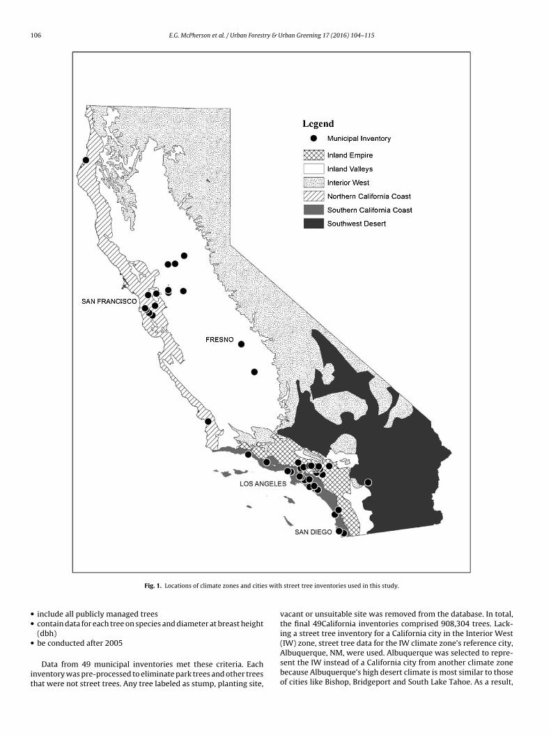
For purposes of i-Tree modeling (McPherson, 2010) Californiawas subdivided into six climate zones based largely on aggregationof Sunset National Garden Book’s 45 climate zones (Brenzel, 1997)and ecoregion boundaries delineated by Bailey (2002) and Breckle(1999) (Fig. 1). Extensive tree size measurements were made in areference city in each climate zone, with growth equations used forbenefit modeling in the i-Tree Streets application (McPherson andPeper, 2012; Peper et al., 2001).

2.2. Street tree inventories

Fifty-six tree inventories were obtained from CAL FIRE, whohas funded inventories and management plans in many Californiacommunities. To be included in this study the inventory had to:

106 E.G. McPherson et al. / Urban Forestry & Urban Greening 17 (2016) 104–115

s with

••

•

it

Fig. 1. Locations of climate zones and citie

include all publicly managed treescontain data for each tree on species and diameter at breast height(dbh)be conducted after 2005

Data from 49 municipal inventories met these criteria. Eachnventory was pre-processed to eliminate park trees and other treeshat were not street trees. Any tree labeled as stump, planting site,

street tree inventories used in this study.

vacant or unsuitable site was removed from the database. In total,the final 49California inventories comprised 908,304 trees. Lack-ing a street tree inventory for a California city in the Interior West(IW) zone, street tree data for the IW climate zone’s reference city,

Albuquerque, NM, were used. Albuquerque was selected to repre-sent the IW instead of a California city from another climate zonebecause Albuquerque’s high desert climate is most similar to thoseof cities like Bishop, Bridgeport and South Lake Tahoe. As a result,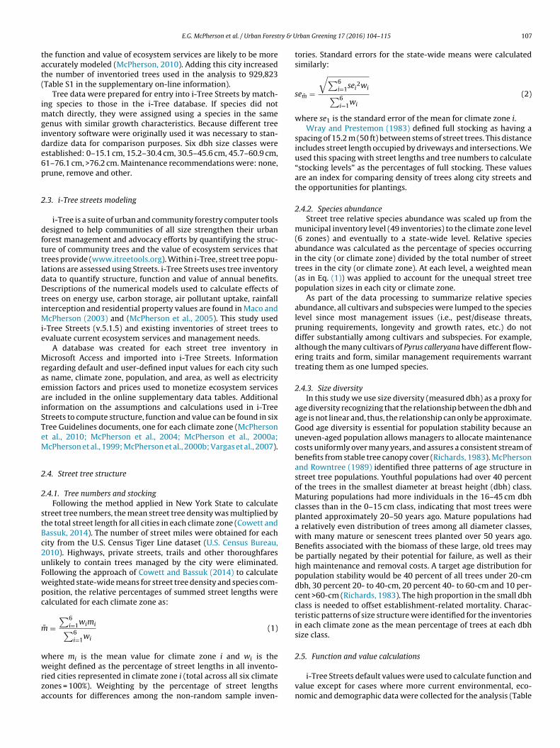

ry & U

tat(

imgide6p

2

dfttldDtiMie

MraeaiSTeM

2

2

stBc2uFwpc

m

wwrza

E.G. McPherson et al. / Urban Forest

he function and value of ecosystem services are likely to be moreccurately modeled (McPherson, 2010). Adding this city increasedhe number of inventoried trees used in the analysis to 929,823Table S1 in the supplementary on-line information).

Tree data were prepared for entry into i-Tree Streets by match-ng species to those in the i-Tree database. If species did not

atch directly, they were assigned using a species in the sameenus with similar growth characteristics. Because different treenventory software were originally used it was necessary to stan-ardize data for comparison purposes. Six dbh size classes werestablished: 0–15.1 cm, 15.2–30.4 cm, 30.5–45.6 cm, 45.7–60.9 cm,1–76.1 cm, >76.2 cm. Maintenance recommendations were: none,rune, remove and other.

.3. i-Tree streets modeling

i-Tree is a suite of urban and community forestry computer toolsesigned to help communities of all size strengthen their urban

orest management and advocacy efforts by quantifying the struc-ure of community trees and the value of ecosystem services thatrees provide (www.itreetools.org). Within i-Tree, street tree popu-ations are assessed using Streets. i-Tree Streets uses tree inventoryata to quantify structure, function and value of annual benefits.escriptions of the numerical models used to calculate effects of

rees on energy use, carbon storage, air pollutant uptake, rainfallnterception and residential property values are found in Maco and

cPherson (2003) and (McPherson et al., 2005). This study used-Tree Streets (v.5.1.5) and existing inventories of street trees tovaluate current ecosystem services and management needs.

A database was created for each street tree inventory inicrosoft Access and imported into i-Tree Streets. Information

egarding default and user-defined input values for each city suchs name, climate zone, population, and area, as well as electricitymission factors and prices used to monetize ecosystem servicesre included in the online supplementary data tables. Additionalnformation on the assumptions and calculations used in i-Treetreets to compute structure, function and value can be found in sixree Guidelines documents, one for each climate zone (McPhersont al., 2010; McPherson et al., 2004; McPherson et al., 2000a;cPherson et al., 1999; McPherson et al., 2000b; Vargas et al., 2007).

.4. Street tree structure

.4.1. Tree numbers and stockingFollowing the method applied in New York State to calculate

treet tree numbers, the mean street tree density was multiplied byhe total street length for all cities in each climate zone (Cowett andassuk, 2014). The number of street miles were obtained for eachity from the U.S. Census Tiger Line dataset (U.S. Census Bureau,010). Highways, private streets, trails and other thoroughfaresnlikely to contain trees managed by the city were eliminated.ollowing the approach of Cowett and Bassuk (2014) to calculateeighted state-wide means for street tree density and species com-

osition, the relative percentages of summed street lengths werealculated for each climate zone as:

¯ =∑6

i=1wimi∑6i=1wi

(1)

here mi is the mean value for climate zone i and wi is the

eight defined as the percentage of street lengths in all invento-

ied cities represented in climate zone i (total across all six climateones = 100%). Weighting by the percentage of street lengthsccounts for differences among the non-random sample inven-

rban Greening 17 (2016) 104–115 107

tories. Standard errors for the state-wide means were calculatedsimilarly:

sem̄ =

√∑6i=1sei

2wi∑6i=1wi

(2)

where se1 is the standard error of the mean for climate zone i.Wray and Prestemon (1983) defined full stocking as having a

spacing of 15.2 m (50 ft) between stems of street trees. This distanceincludes street length occupied by driveways and intersections. Weused this spacing with street lengths and tree numbers to calculate“stocking levels” as the percentages of full stocking. These valuesare an index for comparing density of trees along city streets andthe opportunities for plantings.

2.4.2. Species abundanceStreet tree relative species abundance was scaled up from the

municipal inventory level (49 inventories) to the climate zone level(6 zones) and eventually to a state-wide level. Relative speciesabundance was calculated as the percentage of species occurringin the city (or climate zone) divided by the total number of streettrees in the city (or climate zone). At each level, a weighted mean(as in Eq. (1)) was applied to account for the unequal street treepopulation sizes in each city or climate zone.

As part of the data processing to summarize relative speciesabundance, all cultivars and subspecies were lumped to the specieslevel since most management issues (i.e., pest/disease threats,pruning requirements, longevity and growth rates, etc.) do notdiffer substantially among cultivars and subspecies. For example,although the many cultivars of Pyrus calleryana have different flow-ering traits and form, similar management requirements warranttreating them as one lumped species.

2.4.3. Size diversityIn this study we use size diversity (measured dbh) as a proxy for

age diversity recognizing that the relationship between the dbh andage is not linear and, thus, the relationship can only be approximate.Good age diversity is essential for population stability because anuneven-aged population allows managers to allocate maintenancecosts uniformly over many years, and assures a consistent stream ofbenefits from stable tree canopy cover (Richards, 1983). McPhersonand Rowntree (1989) identified three patterns of age structure instreet tree populations. Youthful populations had over 40 percentof the trees in the smallest diameter at breast height (dbh) class.Maturing populations had more individuals in the 16–45 cm dbhclasses than in the 0–15 cm class, indicating that most trees wereplanted approximately 20–50 years ago. Mature populations hada relatively even distribution of trees among all diameter classes,with many mature or senescent trees planted over 50 years ago.Benefits associated with the biomass of these large, old trees maybe partially negated by their potential for failure, as well as theirhigh maintenance and removal costs. A target age distribution forpopulation stability would be 40 percent of all trees under 20-cmdbh, 30 percent 20- to 40-cm, 20 percent 40- to 60-cm and 10 per-cent >60-cm (Richards, 1983). The high proportion in the small dbhclass is needed to offset establishment-related mortality. Charac-teristic patterns of size structure were identified for the inventoriesin each climate zone as the mean percentage of trees at each dbhsize class.

2.5. Function and value calculations

i-Tree Streets default values were used to calculate function andvalue except for cases where more current environmental, eco-nomic and demographic data were collected for the analysis (Table

1 ry & U

S(mnmgmt

iirrdatSafuaA(

htvtaiarowBpw

raais(

isbePvb

TS

08 E.G. McPherson et al. / Urban Forest

1). To scale-up results from each inventory, mean values per treee.g., kWh cooling savings per tree) were calculated for each cli-

ate zone. The mean values were multiplied by the estimated totalumber of trees and associated measures of variance in each cli-ate zone. Climate zones totals were summed to derive state-wide

rand totals. Standard errors reflect variance associated with esti-ates of tree numbers, and do not include uncertainties related to

ree measurements and numerical modeling.Calculations of energy effects of trees on residential buildings

ncorporated tree species and size data from the inventories. Shad-ng effects were based on the distribution of street trees withespect to buildings recorded from aerial photographs for eacheference city (McPherson and Simpson, 2002). Because theseistributions are unique to each city the values are first-orderpproximations. Energy savings result in reduced emissions of cri-eria air pollutants (volatile organic hydrocarbons [VOCs], NO2,O2, PM10) from power plants and space-heating equipment. Thesevoided emissions were calculated using updated emission factorsor electricity (Table S2) and i-Tree Streets default values for nat-ral gas heating fuel. The updated value of avoided CO2 emissionsssumed a price of $16.53 per t CO2, based on the California Carbonllowance Futures for June 2012 (Climate Policy Initiative, 2014)

Table S3).The uptake of air pollutants by municipal forests can affect

uman health (Nowak et al., 2014). Hourly pollutant dry deposi-ion per tree was calculated using i-Tree Streets default depositionelocities and hourly meteorological data and pollutant concen-rations (Scott et al., 1998). Air quality effects were monetizeds the mean cost of pollution offset transactions (Table S3). Cal-fornia requires air quality management districts that are not inttainment of ambient air quality standards to adopt emissioneduction programs. These programs allow polluters to reduce theirwn emissions to target levels or purchase offsets from pollutersho have already cut their emissions. The California Air Resources

oard’s (2011) most recent report found that 666 transactions tooklace in California in 2008. Mean values that represent the state-ide average cost of a transaction were used in this study.

Intercepted rainfall can evaporate from the tree crown, therebyeducing stormwater runoff. A numerical interception modelccounted for the amount of annual rainfall intercepted by trees,s well as throughfall and stem flow (Xiao et al., 2000). The rainfallnterception benefit was priced by estimating costs of controllingtormwater runoff, and i-Tree Streets default values were usedTable S3).

Many benefits attributed to urban trees are difficult to price (e.g.,ncreased property values, beautification, privacy, wildlife habitat,ense of place, well-being). However, the value of some of theseenefits can be captured in the differences in sales prices of prop-rties that are associated with trees (Anderson and Cordell, 1988).

revious analyses showed that differences in residential propertyalues among cities and associated tree benefits were best modeledy applying the 0.88% sales price increase to the city’s median home

able 1ummary statistics for each climate zone in California (standard error).

Inland Empire Inland Valleys North. Calif. Coast

Street Length (km) 32,940 52,872 35,150

Population 5,818,216 7,263,710 6,738,763

Area (km2) 5074 8275 4431

Trees Sampled 273,351 261,371 147,659

Mean Density (trees/km) 50.74 (6.65) 38.64 (8.02) 56.75 (10.20)

Total Street Trees (1,000s) 1,671.4 (219.0) 2,042.7 (424.1) 1,994.8 (358.4)

Total Sites (1,000s) 4,322.9 6,938.6 4,612.9

Vacant Sites (1,000s) 2,651.5 4,895.9 2,618.1

Full Stocking (%) 38.7 29.4 43.2

Trees per Capita 0.29 (0.04) 0.28 (0.06) 0.30 (0.05)

rban Greening 17 (2016) 104–115

sales price. Hence, in the i-Tree Streets analysis, property valuebenefits ($/tree/year) reflect differences in the contribution to res-idential sales prices of a large front yard tree, and annual changesin leaf area as trees grow in each city. Median home sales priceswere gathered for January to April 2014 (Trulia.com, 2015) (TableS1). Values for ecosystem services are expressed in annual terms,but trees provide benefits across many generations. To enable treeplanting and stewardship to be seen as a capital investment, thereplacement value of all street trees was calculated by i-Tree Streetsfollowing trunk formula procedures outlined by the Council of Treeand Landscape Appraisers (2000) .

3. Results

3.1. Sample

The total population of inventoried cities (4.5 million) is 14.8% ofCalifornia’s 30.8 million people living in cities (Table 1). Another 6.4million Californians live in unincorporated areas, but there were notree inventory data for counties. There are differences in percent-ages of population, street length, city area and street tree inventorynumbers across climate zones. For example, 13.3 million peopleliving in cities in the Southern California Coast (SC) climate zoneaccount for 38.5% of the state’s inhabitants. However, because pop-ulation density is relatively high, the percentages of street length(27.6%) and land area (21.2%) are substantially less than popula-tion. Conversely, population densities are lowest in the SouthwestDesert (SW) and Interior West (IW) zones, where percentages ofstreet length and land area are several times greater than theirrespective population percentages.

3.2. Structure

3.2.1. Tree numbers and stockingThe weighted mean street tree density is 46.6 (3.5 standard error

[se]) trees per km street length (75.0/mile, 5.7 se) and ranges from6.6 (IW, 10.6/mile) to 56.8 per km (Northern California Coast [NC],91.3/mile). There are approximately 9.1 million street trees in Cal-ifornia cities (Table 1) and 0.26 street trees per capita, about onestreet tree for every four persons. State-wide, city streets are at36.3% of full stocking and there are approximately 16 million vacanttree sites.

The SC zone has 30.3% of all California street trees, but the num-ber of trees per capita, 0.21 (about 1 street tree for every 5 people),is relatively low. Cities in the Inland Valley (IV) and NC zones con-tain 22.4% and 21.8% of all trees, respectively. The numbers of treesper capita are similar, 0.28 and 0.30. Street trees in the IE accountfor 18.3% of the state-wide total and there are 0.29 trees per capita.

The estimated 631,146 street trees in the SW zone account for 6.8%of the state-wide total and there are 0.5 trees per capita. Cities inthe IW zone had an estimated 25,516 trees (0.3%) and 0.13 treesper capita.

South. Calif. Coast Southwest Desert Interior West Total

33,607 16,766 4032 195,84513,339,610 1,250,997 211,054 34,622,3506028 3643 1049 28,499215,624 10,299 21,519 929,82351.09 (6.11) 37.64 (6) 6.58 (1.04) 46.62 (3.52)2,763.3 (330.4) 631.1 (100.7) 26.5 (4.2) 9,129.8 (689.7)7,097.8 2,200.3 529.1 25,172.44,334.5 1,569.1 502.6 16,042.638.9 28.7 5.0 36.30.21 (0.02) 0.50 (0.08) 0.13 (0.02) 0.26 (0.02)

E.G. McPherson et al. / Urban Forestry & Urban Greening 17 (2016) 104–115 109

Table 2Relative species abundance (%) by climate zone and statewide. Species are listed in descending order of relative abundance.

Inland Empire % Inland Valleys % North. Calif.Coast

% South. Calif.Coast

% Southwest Desert % California %

Lagerstroemia indica 9.4 Platanus xhispanica

11.3 Platanus xhispanica

10.5 Pinus canariensis 6.3 Washingtoniarobusta

18.0 Platanus xhispanica

10.5

Liquidambar styraciflua 9.3 Pistacia chinensis 8.9 Magnoliagrandiflora

7.0 Lophostemonconfertus

4.8 Washingtoniafilifera

9.3 Pistacia chinensis 7.0

Cinnamomum camphora 4.5 Lagerstroemiaindica

6.9 Liquidambarstyraciflua

6.6 Washingtoniarobusta

4.4 Phoenixdactylifera

6.8 Lagerstroemiaindica

6.6

Pinus canariensis 4.2 Pyrus calleryana 5.2 Pyrus calleryana 3.7 Lagerstroemiaindica

4.2 Dalea spinosa 4.9 Pyrus calleryana 3.7

Platanus x hispanica 4.2 Celtis sinensis 4.5 Pistacia chinensis 3.4 Liquidambarstyraciflua

4.0 Acacia aneura 4.5 Liquidambarstyraciflua

3.4

Syagrus romanzoffiana 3.5 Fraxinus velutina 3.6 Lagerstroemiaindica

3.2 Jacarandamimosifolia

3.7 Parkinsoniaflorida

3.8 Celtis sinensis 3.2

Pyrus calleryana 2.8 Zelkova serrata 3.6 Prunus cerasifera 3.1 Eucalyptusglobulus

3.5 Acaciastenophylla

3.6 Fraxinus velutina 3.1

Washingtonia robusta 2.8 Liquidambarstyraciflua

3.0 Quercus agrifolia 3.1 Magnoliagrandiflora

3.1 Acacia farnesiana 3.6 Magnoliagrandiflora

3.1

Magnolia grandiflora 2.7 Sequoiasempervirens

2.9 Cinnamomumcamphora

2.9 Syagrusromanzoffiana

2.8 Brachychitonpopulneus

3.3 Zelkova serrata 2.9

2.7

214

3

m(m

roatwodc

sTcpflvzc

bttr

3

riIoaSft

3

u

Ulmus parvifolia 2.7 Magnoliagrandiflora

2.6 Fraxinus velutina

Mean # taxa 174 157

.2.2. Species abundanceThe relative abundance of the top species is listed for each cli-

ate zone, as well as the mean number of taxa in the inventoriesTable 2). The mean number of taxa for California is 175 and the

eans range from 105 (SW) to 214 (NC) among climate zones.In the SW climate zone California fan palm (Washingtonia

obusta) is by far the most abundant species (18%), followed by twother palm species: Mexican fan palm (Washingtonia filifera) at 9.3%nd date palm (Phoenix dactylifera) at 6.8%. The climate zones withhe next highest single species abundance are the IV and the NC,here London planetree (Platanus x hispanica) accounts for 10.5%

f all trees. Of all the climate zones, SC has the lowest relative abun-ance of a top species, with Canary Island pine (Pinus canariensis)omprising 6.3% of the street tree population.

On the state-wide scale, London planetree (10.5%) is the solepecies that claimed more than 10% relative abundance (Table 2).he next most abundant species are Chinese pistache (Pistaciahinensis, 7.0%), crape myrtle (Lagerstroemia indica, 6.6%), Calleryear (Pyrus calleryana, 3.7%) and sweetgum (Liquidambar styraci-ua, 3.4%). Chinese hackberry (Celtis sinensis), velvet ash (Fraxinuselutina), Southern magnolia (Magnolia grandiflora), Japaneseelkova (Zelkova serrata) and redwood (Sequoia sempervirens) eachomprise about 3% of the state’s street tree population.

Besides Canary Island pine, which is present in substantial num-ers in the SC and IE, the only other coniferous species in the topen most abundant species is redwood (2.7% in the IV). State-wide,hese two conifers make up nearly 4% of the street tree population’selative abundance.

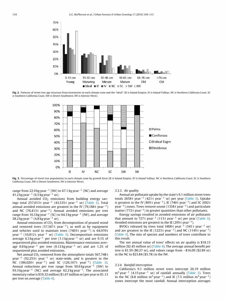
.2.3. Size diversityThe IV inventories are characterized as young populations, with

elatively high percentages of young trees (55%) and lower thandeal percentages of mature (18%) and old (5%) trees (Fig. 2). TheE and SW populations are mature, with above ideal percentagesf mature trees (37%) and relatively few young trees (26%). The SCnd NC have nearly ideal percentages of young trees (35%), but theC has above ideal percentages of mature trees (33%) and relativelyew old trees (5%). The mean percentages for the NC come closesto matching the ideal distribution of age diversity.

.2.4. Life formIn the IW, IV and NC over 60% of inventoried trees are decid-

ous (Fig. 3). In the IE inventories, deciduous (44%) and broadleaf

Cupaniopsisanacardioides

2.8 Chilopsis linearis 2.7 Sequoiasempervirens

2.7

171 105 175

evergreens (39%) account for 83% of their populations. In the SCinventories, 50% of all trees are broadleaf evergreens. Palms (35%)are the most abundant life form in the SW inventory, followedclosely by broadleaf evergreens (31%) and deciduous (30%).

3.2.5. MaintenanceTree maintenance recommendations were reported in 44 of the

49California inventories. The mean percentage of trees requiringpruning range from 63.4% in the IV to 94.8% in the NC. In the IE andSC the mean values are 89.1% and 90.9%, respectively. The mean per-centage of trees requiring removal range from 1.2% (IV) to 3.3% (IE).Mean values are 1.5% and 2.0% for the SC and NC zones, respectively.

3.3. Function and value

3.3.1. EnergyState-wide annual electricity savings from air conditioning

reductions total 684 GWh year−1 (114 GWh year−1 se), or 74.9 kWhyear−1 per tree (12.5 se) on average (Table 3). Cooling savings aver-age 90–100 kWh year−1 per tree in the NC, IV, and IE climate zones,and total 200, 186 and153 GWh year−1, respectively.

State-wide, street trees reduce annual natural gas used for heat-ing by 580,152 GJ year−1 (100,049 GJ year−1 se), or 60.2 kBtu year−1

per tree on average (Table 3). Trees slightly increase heating in theIE zone by −35,921 GJ year−1 (−20 kBtu year−1 per tree). Heatingsavings are greatest in the NC zone (427,326 GJ year−1, 203 kBtuyear−1 per tree).

The total annual monetary value of energy savings from thestate’s 9.1 million street trees is $101.15 million ($16.8 million se)(Table 4). The average annual benefit per tree is $11.08 ($1.84 se)and ranges from $5.77 in the SC to $15.68 in the NC.

3.3.2. Carbon dioxideCalifornia’s 9.1 million street trees are estimated to store 7.78

million metric tonnes (MMt) (1.3 MMt se) CO2 (Table 3). Climatezones wherein the most CO2 is stored in street tree biomass are theNC (2.51 MMt) and IV (2.17MMt). On average, 852.4 kg (142.1 kg)CO2 is stored per tree. The average amount stored per tree is nearlyfour times greater in the NC (1,256.3 kg) than the SW (327.6 kg).

The amount of CO2 sequestered each year by street treesis 375,704 t year−1 (59,530 t year−1 se) (Table 3). Municipalforests in the NC (133,772 t year−1) and SC (94,961 t year−1)zones sequester the most CO2. Sequestration rates per tree

110 E.G. McPherson et al. / Urban Forestry & Urban Greening 17 (2016) 104–115

Fig. 2. Patterns of street tree age structure from inventories in each climate zone and the “ideal” (IE is Inland Empire, IV is Inland Valleys, NC is Northern California Coast, SCis Southern California Coast, SW is Desert Southwest, IW is Interior West).

F (IE is

C

r4

iaar2

aayasas

yNA9mp

ig. 3. Percentage of street tree populations in each climate zone by growth form

alifornia Coast, SW is Desert Southwest, IW is Interior West).

ange from 22.9 kg year−1 (IW) to 67.1 kg year−1 (NC) and average1.2 kg year−1 (6.5 kg year−1 se).

Annual avoided CO2 emissions from building energy sav-ngs total 257,013 t year−1 (43,535 t year−1 se) (Table 3). Totalnnual avoided emissions are greatest in the IV (79,188 t year−1)nd NC (76,413 t year−1). Annual avoided emissions per treeange from 16.3 kg year−1 (SC) to 64.3 kg year−1 (IW), and average8.2 kg year−1 (4.8 kg year−1 se).

Annual emissions of CO2 from decomposition of pruned woodnd removed trees (57,567 t year−1), as well as by equipmentnd vehicles used to maintain trees (7403 t year−1) is 64,970 tear−1 (10,812 t year−1 se) (Table 3). Decomposition emissionsverage 6.3 kg year−1 per tree (1.1 kg year−1 se) and are 9.1% ofequestered plus avoided emissions. Maintenance emissions aver-ge 0.8 kg year−1 per tree (0.12 kg year−1 se) and are 1.2% ofequestered plus avoided emissions.

Net annual CO2 removed from the atmosphere totals 567,748 tear−1 (92,253 t year−1 se) state-wide, and is greatest in theC (186,020 t year−1) and SC (126,167 t year−1) (Table 3).

−1

nnual reductions per tree range from 50.6 kg year (SW) to3.3 kg year−1 (NC) and average 62.2 kg year−1. The associatedonetary value is $10.32 million ($1.67 million se) per year or $1.13

er tree on average (Table 4).

Inland Empire, IV is Inland Valleys, NC is Northern California Coast, SC is Southern

3.3.3. Air qualityAnnual air pollutant uptake by the state’s 9.1 million street trees

totals 2658 t year−1 (421 t year−1 se) per year (Table 3). Uptakeis greatest in the IV (805 t year−1), IE (740 t year−1) and SC (692 tyear−1) zones. Trees remove ozone (1358 t year−1) and particulatematter (772 t year−1) in greater quantities than other pollutants.

Energy savings resulted in avoided emissions of air pollutantsthat amount to 727 t year−1 (113 t year−1 se) per year (Table 3).Avoided emissions are greatest in the IE (295 t year−1).

BVOCs released by trees total 3400 t year−1 (541 t year−1 se)and are greatest in the IE (1223 t year−1) and NC (1145 t year−1)(Table 3). The mix of species and numbers of trees contribute tothis result.

The net annual value of trees’ effects on air quality is $18.15million ($2.45 million se) (Table 4). The average annual benefit pertree is $1.59 ($0.27 se), and values range from −$16.09 ($2.89 se)in the NC to $23.84 ($3.78) in the IW.

3.3.4. Rainfall interception

California’s 9.1 million street trees intercept 26.19 million

m3 year−1 (4.15 year−1 se) of rainfall annually (Table 3). Treesin the NC (8.8 million m3 year−1) and IE (7.5 million m3 year−1)zones intercept the most rainfall. Annual interception averages

E.G. McPherson et al. / Urban Forestry & Urban Greening 17 (2016) 104–115 111

Table 3Functional services produced by the street tree population in each climate zone and statewide.

Resource Units Inl. Empire Inl. Valleys North. Coast South. Coast SW Desert Int. West Total

EnergyCooling 153 (20) 186 (39) 200 (36) 101 (12) 42 (7) 2 (0) 684 (114)Heating −35.9 (4.7) 44.6 (9.3) 427.3 (76.8) 106.9 (12.8) 31.4 (5.0) 5.8 (0.9) 580.2 (100.0)CO2Stored 1361 (178) 2174 (451) 2506 (450) 1517 (181) 207 (33) 18 (3) 7782 (1297)Sequestered 73.6 (9.6) 58.0 (12.0) 133.7 (24.0) 95.0 (11.4) 14.8 (2.4) 0.6 (0.1) 375.7 (59.5)Avoided 35.8 (4.7) 79.2 (16.4) 76.4 (13.7) 44.9 (5.4) 19.0 (3.0) 1.7 (0.3) 257.0 (43.5)Released Decomp. −1.3 (0.2) −15.3 (3.2) −24.1 (4.3) −15.2 (1.8) −1.7 (0.3) −0.1 (0.02) −57.6 (9.8)Released Maint. −4.4 (0.6) −1.1 (0.2) −0.1 (0.02) −1.5 (0.2) −0.2 (0.03) −0.01 (0.00) −7.4 (1.1)Net Total 103.7 (13.6) 120.8 (25.1) 186.0 (33.4) 123.2 (14.7) 31.9 (5.1) 2.2 (0.3) 567.8 (92.3)Air QualityDeposition O3 378 (49) 443 (92) 166 (30) 339 (41) 28 (4) 4 (1) 1358 (217)Deposition NO2 141 (18) 112 (23) 68 (12) 149 (18) 14 (2) 1 (0) 485 (74)Deposition PM10 207 (27) 250 (52) 96 (17) 191 (23) 27 (4) 1 (0) 772 (124)Deposition SO2 15 (2) 0 (0) 13 (2) 12 (1) 3 (0) 0 (0) 43 (6)Total Deposition 740 (97) 805 (167) 343 (62) 692 (83) 72 (11) 6 (1) 2658 (421)Avoided NO2 85 (11) 93 (19) 50 (9) 57 (7) 34 (5) 4 (1) 324 (52)Avoided PM10 21 (3) 18 (4) 13 (2) 14 (2) 2 (0) 1 (0) 68 (11)Avoided SO2 168 (22) 43 (9) 26 (5) 27 (3) 29 (5) 3 (1) 296 (44)Avoided VOC 21 (3) 5 (1) 6 (1) 6 (1) 0 (0) 1 (0) 39 (6)Total Avoided 295 (39) 159 (33) 96 (17) 104 (12) 65 (10) 9 (1) 727 (113)Released BVOC −1223 (160) −531 (110) −1145 (206) −390 (47) −108 (17) −4 (1) −3400 (541)Net Total −188 (25) 433 (90) −707 (127) 397 (48) 29 (5) 11 (2) −25 (8)StormwaterInterception 7498 4144 8840 4674 985 45 26,186(se) (983) (860) (1588) (559) (157) (7) (4154)

Units: Cooling (GWh/yr), Heating (MJ/yr), Stored CO2 (1,000 t), Units: Sequestered, Avoided, Released, Net CO2 (1000 t/yr), Air Quality (1 metric tonne/yr), Interception(1000 m3/yr).

Table 4Annual monetary value (in million $US) of street tree services by climate zone and statewide (se).

Service Inland Empire Inland Valleys North. Calif. Coast South. Calif. Coast Southwest Desert Interior West Total

Energy 21.37 (2.80) 25.73 (5.34) 31.27 (5.62) 15.95 (1.91) 6.54 (1.04) 0.28 (0.04) 101.15 (16.76)Carbon Dioxide 1.95 (0.26) 2.13 (0.44) 3.28 (0.59) 2.36 (0.28) 0.56 (0.09) 0.04 (0.01) 10.32 (1.67)Air Quality 0.60 (0.08) 23.64 (4.91) −32.09 (5.77) 23.01 (2.75) 2.37 (0.38) 0.63 (0.10) 18.15 (2.45)

2(

wa$

3

v((e$

3

mbi

3

mso

Stormwater 14.26 (1.87) 8.32 (1.73) 9.34 (1.68)

Property Value/Other 150.48 (19.72) 108.36 (22.50) 299.42 (53.80)

Total 188.67 (24.73) 168.18 (34.92) 311.20 (55.92)

.87 m3 year−1 per tree (0.46 se) and ranges from 1.56 m3 year−1

SW) to 4.49 m3 year−1 (IE).The monetary value of rainfall interception totals $41.5 million,

ith the greatest benefit in the IE ($14.26 million) (Table 4). Theverage annual benefit per tree is $4.55 ($0.71 se) and ranges from1.98 (SW) to $8.53 (IE).

.3.5. Property values and other benefitsStreet trees contribute to the sales prices of homes and pro-

ide other benefits valued at $838.94 million ($130.9 se) per yearTable 4). Property values and other benefits are largest in the NC$299.4 million) and SC ($246.6 million) zones. Average annual ben-fits per tree range from $16.19 (IW) to $150.09 (NC) and average91.89 ($14.34 se).

.3.6. Total annual benefitsThe total annual value of street tree services is $1.0 billion ($58.3

illion se), or $110.63 per tree ($17.34 se) (Table 4). Total annualenefits are $311.2 ($156.0 per tree) and $296.1 ($107.17 per tree)

n the NC and SC zones, respectively.

.3.7. Replacement value

The replacement value for all street trees is $2.49 billion ($7.96

illion se) (Table 4). This amount is the asset value of the state’street trees when considered as a capital investment similar tother infrastructure. It averages to $2677 per tree ($108.90 se).

8.27 (0.99) 1.25 (0.20) 0.06 (0.01) 41.50 (6.47)246.56 (29.48) 33.70 (5.37) 0.43 (0.07) 838.94 (130.94)296.14 (35.41) 44.42 (7.08) 1.44 (0.23) 1,010.05 (158.29)

4. Discussion

California has approximately 9.1 million street trees, about onefor every four city resident. To fill the vacant street tree sites wouldrequire planting 16 million trees. Assuming that 50% of these arereadily plantable, it appears feasible to nearly double the state’sstreet tree population through planting of another 8 million vacantstreet tree sites. State-wide, species diversity is good, with onlyLondon planetree accounting for over 10% of the population. Theannual value of street tree services is $1.0 billion, or $110.63 pertree ($29.17 per capita). These findings contribute new knowledgeon the structure, function and value of street trees in California.

4.1. Structure

McPherson and Simpson (2003) reported that there were 177.3million trees in urban areas in California. Assuming this numberis still valid, the state’s 9.1 million street trees account for about5% of the urban forest. This study’s findings indicate that the trendof increasing street tree numbers reported by Thompson (2006) iscontinuing, although the use of different methodologies limits theconclusiveness of these comparisons. In 1988 there were approx-imately 5.9 million street trees (0.26 per capita) and the number

increased to 7.2 million trees (0.29 per capita) in 2003. The 9.1 mil-lion street trees reported here continues the increasing trend intree numbers, while the 0.26 trees per capita is a slight decreasefrom 2003. Thompson (2006) reported a rapid increase in planting

112 E.G. McPherson et al. / Urban Forestry & Urban Greening 17 (2016) 104–115

Table 5For each climate zone, the number of cities in which the most dominant species account for a percentage of total zone-wide species and genus. Total number of inventoriesin parentheses.

Species Genus

Climate zone <10% 10–15% 15–20% 20–30% >30% <10% 10–15% 15–20% 20–30% >30%Inl. Empire (17) 3 7 5 2 0 1 6 7 3 0Inl. Valleys (8) 1 4 2 1 0 1 3 3 1 0North Coast (8) 2 5 1 0 0 1 6 1 0 0

itiamsrv1

i((MespSddfgS

tacscfn

lN2MnetuttnwrteL

opcmP

South Coast (15) 4 7 3 1

SW Desert (1) 0 0 1 0

California (49) 1 0 0 0

n the late-1980s and early-1990s, but this trend began to erode inhe mid-1990s. However, California had a number of tree plantingnitiatives during the past decade that were funded through voter-pproved bond measures. The current ratio of 0.26 trees per capitaatches the value reported for 1988, suggesting that the trend is

table. It should be noted that these ratios are less than the 0.38eported for California in 1979 (Kielbaso et al., 1988) and the meanalue of 0.37 reported for 22 U.S. cities (McPherson and Rowntree,989).

Average street tree density in California (46.6/km, 75.0/mile)s less than 50.0 per km (80.5/mile) reported for New YorkCowett and Bassuk, 2014), but greater than 28.6 (46/mi.), 36.058/mi.), 37.3 (60/mi.) and 39.1 (63/mi) reported for Maryland,

assachusetts, Missouri and Wisconsin, respectively (Cummingt al., 2008; Cumming et al., 2006; Gartner et al., 2002). It is a sub-tantial reduction from 65.6 (105.5/mi.) and 64.3 (103.5/mi.) treeser km reported for California in 1988 and 1992 (Bernhardt andwiecki, 1989, 1993), respectively. One possible explanation for thisownward trend is that street tree planting rates are lagging behindevelopment of new streets. Another factor could be that relatively

ew removed trees are being replaced. In 1992, 15% of surveyed pro-rams were removing more trees than they planted (Bernhardt andwiecki, 1993). In 2003, this increased to 22% (Thompson, 2006).

The ideal urban forest is not dominated by a few species. Rather,ree numbers are distributed fairly evenly among dozens of well-dapted species. Species diversity protects a community’s treeanopy cover by limiting the amount of damage from any one threatuch as pests, drought or storms (McPherson and Kotow, 2013). Aommonly accepted diversity goal is for no single species to accountor more than 10% of the population, no genus more than 20% ando family more than 30% (Santamour, 1990).

The absence of diversity has been reported at state-wide andocal scales (Ball et al., 2007; Raupp et al., 2006). For example,orway maple (Acer platanoides) accounted for 34%, 31%, 21% and0.7% of all street trees in the states of Massachusetts, Wisconsin,ichigan and New York, respectively. This lack of diversity was

ot the case for California. At the state-wide scale, London plan-tree was the most abundant species accounting for 10.5% of allrees (Table 2). The Platanus genus comprised only 10% of the pop-lation. Hence, no single genus accounted for more than 20% ofhe population (Table 5). However, the need for further diversifica-ion was evident at the city and climate zone scales. The metric ofo single species accounting for more than 10% of the populationas exceeded in 3 climate zones and 36 of the municipal invento-

ies. The metric of no single genus accounting for more than 20% ofhe population was exceeded in 4 climate zones and 8 cities. Gen-ra that exceeded the 20% target at the city scale were Eucalyptus,agerstroemia, Quercus, Pistacia, Pinus and Washingtonia.

Overreliance on the London planetree was identified as a seri-us concern in California because of its vulnerability to severe

ests such as the granulate ambrosia beetle (Xylosandrus crassius-ulus), Asian longhorned borer and Armillaria root rot (caused byembers of the genus Armillaria) (McPherson and Kotow, 2013).

lanting of this species and other overly abundant and highly vul-

0 2 7 3 2 10 0 0 0 1 00 1 0 0 0 0

nerable species such as sweetgum, Chinese pistache, velvet ash andCallery pear could be reduced. Ongoing evaluation of climate-readyspecies that are also compatible to street-side conditions is needed(McPherson and Berry, 2015).

The results from this study support the notion that growth formsreflect environmental conditions (McPherson and Rowntree, 1989).Deciduous trees prevail in the more temperate climate zones (IW,IV, NC), while broadleaf evergreens and palms predominate in thesubtropical climate zones (SC, SW). Conifers are relatively unim-portant along California streets, regardless of climate zone.

The age structure of street trees in California is younger thanreported for Maryland, Massachusetts and Missouri. For example,in these states less than 20% of all trees are in the smallest dbhsize class. In California climate zones this number ranges from26% to 55%. The preponderance of small sized trees may reflecta relatively youthful state-wide population. Alternatively, it couldreflect recent planting of many small-stature trees that may nevergrow out of the 0–15 cm dbh class. Further investigation is neededto identify the species composition and mature ages and sizes ofrecently planted tree species.

4.2. Function and value

Street tree population function has been reported for the Cali-fornia cities of Modesto, Santa Monica and Berkeley (McPhersonand Simpson, 2002; McPherson et al., 2005). The annual mone-tary values of street tree services were reported for the states ofMissouri (Treiman et al., 2011a), Indiana (Davey Resource Group,2010a) and Wisconsin (Cumming et al., 2008). For comparison pur-poses, results were divided by total tree numbers and presented pertree except for Wisconsin, where data were missing for many ser-vices (Table 6). Because results are all from the same i-Tree Streetsmodel they are comparable. Differences among states reflect theeffects of different street tree structures, climate zones and modelinputs such as local prices for ecosystem services.

The 684 GWH of electricity saved annually by California’sstreet trees is equivalent to the amount required to air condition530,000California households each year (4.4% of 12.2 million). Theaverage per tree amount of 74.9 kWh falls within the range of valuesreported for other California cities (36–138 kWh). Average annualenergy savings of $11.08 per street tree for California is more than$6.83 in Indiana and less than $32.71 in Missouri.

Approximately 7.78 million t CO2 is stored in the state’s 9.1million street trees. They remove and avoid 567,748 t of CO2 emis-sions annually, equivalent to removing 120,000 cars from theroad. On an average annual per tree basis, street trees sequesterand avoid 34.7 and 28.2 kg of CO2, respectively. The amountsequestered is less than values previously reported for Californiacities (41–96 kg year−1) and the amount avoided falls within the

range reported in other states and cities (18–36 kg year−1). Theaverage annual value of CO2 removal is $1.13 per tree, more than$0.20 and $0.82 in Wisconsin and Indiana, but less than $2.75 inMissouri.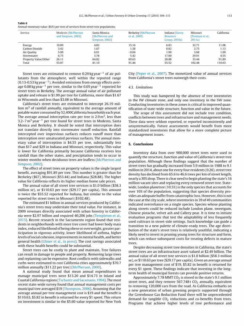

E.G. McPherson et al. / Urban Forestry & Urban Greening 17 (2016) 104–115 113

Table 6Annual monetary value ($US) per tree of services from street tree populations.

Service Modesto (McPhersonand Simpson, 2002)

Santa Monica(McPherson andSimpson, 2002)

Berkeley (McPhersonet al., 2005)

Indiana (DaveyResourceGroup, 2010a)

Missouri(Treiman et al.,2011a)

California

Energy 10.89 4.82 15.16 6.83 32.71 11.08Carbon Dioxide 3.42 1.67 1.28 0.82 2.75 1.13Air Quality 5.90 6.01 −0.04 1.99 3.68 1.99

l(asui

lpT3MniietirwS

bBv

mir

n2n2ditlgw

cacm

mCrma$o

Stormwater 6.75 3.78

Property Value/Other 26.11 64.82

Total 53.07 81.10

Street trees are estimated to remove 0.29 kg year−1 of air pol-utants from the atmosphere, well within the reported range0.13-0.53 kg year−1). Avoided emissions from energy effects aver-ge 0.08 kg year−1 per tree, similar to the 0.05 year−1 reported fortreet trees in Berkeley. The average annual value of air pollutantptake and release is $1.99 per tree for California, more than $1.67

n Wisconsin and less than $3.68 in Missouri.California’s street trees are estimated to intercept 26.19 mil-

ion m3 of rainfall annually, equivalent to the average amount ofotable water consumed by 52,400California households each year.he average annual interception rate per tree is 2.9 m3, less than.2–7 m3 year−1 per tree found for street trees in Modesto, Santaonica and Berkeley. It should be noted that interception does

ot translate directly into stormwater runoff reduction. Rainfallntercepted over impervious surfaces reduces runoff more thannterception over unsaturated pervious surfaces. The annual mon-tary value of interception is $4.55 per tree, substantially lesshan $17 and $29 in Indiana and Missouri, respectively. This values lower for California primarily because California receives lessainfall than the other states, and precipitation tends to occur ininter months when deciduous trees are leafless (McPherson and

impson, 2002).The effect of street trees on property values is the single largest

enefit, averaging $91.89 per tree. This number is greater than forerkeley ($67), Missouri ($53.44) and Indiana ($28.88). The higheralue for California reflects its higher median home sale prices.

The annual value of all street tree services is $1.0 billion ($58.3illion se), or $110.63 per tree ($29.17 per capita). This amount

s twice the $55.52 reported for Indiana, but similar to the valueeported for street trees in Missouri ($102.48).

The estimated $1 billion in annual services produced by Califor-ia’s street trees may understate their total value. For instance, in009 revenues directly associated with urban forestry in Califor-ia were $2.97 billion and required 40,206 jobs (Templeton et al.,013). Recent research in the Sacramento region found that resi-ents in neighborhoods with more tree cover had lower body mass

ndex, reduced likelihood of being obese or overweight, greater par-icipation in vigorous activity, lower likelihood of asthma, higherevels of social cohesion, improvements in mental health, and bettereneral health (Ulmer et al., in press). The cost savings associatedith these health benefits could be substantial.

Street trees can be costly to plant and maintain. Tree failuresan result in damage to people and property. Removing large treesnd replanting can be expensive. Root conflicts with sidewalks andurbs were estimated to cost California cities approximately $70.7illion annually ($11.22 per tree) (McPherson, 2000).

A national study found that mean annual expenditures toanage municipal trees were $13.20 and $14.73 in Inland and

oastal California regions (Tschantz and Sacamano, 1994). The mostecent state-wide survey found that annual management costs per

unicipal tree averaged $19 (Thompson, 2006). Assuming that theverage annual per tree management cost is $19 and the benefit is110.63, $5.82 in benefit is returned for every $1 spent. This returnn investment is similar to the $5.60 value reported for New York

5.42 17.00 29.91 4.5569.63 28.88 33.44 91.8991.44 55.52 102.48 110.63

City (Peper et al., 2007). The monetized value of annual servicesfrom California’s street trees outweigh their costs.

4.3. Limitations

This study was hampered by the absence of tree inventoriesin the IW climate zone, and only one inventory in the SW zone.Conducting inventories in these zones is critical to improved quan-tification of state-wide structure, function and value in the future.

The scope of this assessment did not include tree condition,conflicts between trees and infrastructure and management needs.These data were seldom reported, or reported inconsistently andunsystematically. Future assessments would benefit from morestandardized inventories that allow for a more complete pictureof management issues.

5. Conclusions

Inventory data from over 900,000 street trees were used toquantify the structure, function and value of California’s street treepopulation. Although these findings suggest that the number ofstreet trees has gradually increased from 5.9 million in 1988 to 9.1million in 2014, about one for every four residents (0.26), street treedensity has declined from 65.6 to 46.6 trees per km of street length,nearly a 30% drop. There is clear need to begin planting the state’s 16million vacant sites and replacing every removed street tree. State-wide, London planetree (10.5%) is the only species that accounts forover 10% of the population, suggesting that species diversity pro-vides an adequate buffer from catastrophic loss. However, this is notthe case at the city scale, where inventories in 39 of 49 communitiesindicated overreliance on a single species. Species whose plantingalong streets could be reduced include London plane, sweetgum,Chinese pistache, velvet ash and Callery pear. It is time to initiateevaluation programs that test the adaptability of less frequentlyused cultivars in street-side settings. Such knowledge can guide atransition to a new palette of climate-ready trees. The age distri-bution of the state’s street trees is relatively youthful, indicating alikely need to invest in pruning young trees for structure and form,which can reduce subsequent costs for treating defects in maturetrees.

Despite decreasing street tree densities in California, the state’sstreet trees are an infrastructure asset valued at $2.49 billion. Theannual value of all street tree services is $1.0 billion ($58.3 millionse), or $110.63 per tree ($29.17 per capita). Given an average annualper tree management cost of $19, $5.82 in benefit is returned forevery $1 spent. These findings indicate that investing in the long-term health of municipal forests can provide positive returns.

Approximately 7.78 MMT CO2 is stored in the state’s 9.1 millionstreet trees, and they remove 567,748 t CO2 annually, equivalentto removing 120,000 cars from the road. As California embarks on

a new generation of urban greening projects supported throughthe Greenhouse Gas Reduction Fund there will be unprecedenteddemand for tangible CO2 reductions and co-benefits from trees.Programs that achieve higher levels of tree performance and

1 ry & U

dwmmttf

A

wTJDFd

A

i0

R

A

B

B

B

B

BBC

C

C

C

C

C

D

D

G

J

K

K

L

14 E.G. McPherson et al. / Urban Forest

evelop more sophisticated monitoring and reporting protocolsill be rewarded. To that end, this study presents actionableanagement recommendations to reverse undesirable trends anditigate threats to future tree health and performance. Also,

hese findings provide an important baseline from which to gaugehe effectiveness of future investments in California’s municipalorests.

cknowledgements

We are deeply indebted to the many partners who assistedith this study. These collaborators include Drs. Jim Quinn and Jim

horne at the UC Davis Information Center for the Environment andohn Melvin, Chris Keithley and Mary Klaus Schulz with CAL FIRE.r. Qingfu Xiao (UC Davis), Paula Peper and Shannon Albers (USDAorest Service, PSW Research Station) provided technical supporturing portions of the study.

ppendix A. Supplementary data

Supplementary data associated with this article can be found,n the online version, at http://dx.doi.org/10.1016/j.ufug.2016.03.13.

eferences

nderson, L.M., Cordell, H.K., 1988. Influence of trees on residential propertyvalues in Athens, Georgia: a survey based on actual sales prices. LandscapeUrban Plann. 15, 153–164.

ailey, R.G., 2002. Ecoregion-based Design for Sustainability. Springer-Verlag, NewYork, NY.

all, J., Mason, S.J., Kiesz, A., McCormick, D., Craig, B., 2007. Assessing the hazard ofemerald ash borer and other exotic stressors to community forests. Arboric.Urban For. 33, 350–359.

ernhardt, E., Swiecki, T.J., 1989. The state of urban forestry in California. In:Results of the 1988 California Urban Forest Survey. California Department ofForestry and Fire Protection, Sacramento, CA, pp. p. 68.

ernhardt, E., Swiecki, T.J., 1993. The State of Urban Forestry in California – 1992.California Department of Forestry and Fire Protection, Sacramento, CA, pp. p.61.

reckle, S.W., 1999. Walter’s Vegetation of the Earth, 4th ed. Springer, Berlin.renzel, K., 1997. Sunset National Garden Book. Sunset Books, Inc., Menlo Park, CA.alifornia Air Resources Board, 2011. Emission Reduction Offset Transaction Costs

Summary Report for 2008, http://www.arb.ca.gov/nsr/erco/erc08.pdf(accessed 08.12.14).

limate Policy Initiative, 2014. California Carbon Dashboard, http://calcarbondash.org/ (accessed 08.12.14).

ouncil of Tree and Landscape Appraisers, Guide for Plant Appraisal (9th ed.).International Society of Arboriculture, Champaign, IL, 2000.

owett, F., Bassuk, N., 2014. State-wide assessment of street trees in new Yorkstate, USA. Urban For. Urban Greening 13, 213–220.

umming A.B., Twardus D.B., Smith W.D., National forest health monitoringprogram: Maryland and Massachusetts street tree monitoring pilot projects.NA-FR-01-06. United States Department of Agriculture, Forest Service,Northeastern Area State and Private Forestry, p. 23. 2006.

umming A.B., Twardus D.B., Hoehn R., Nowak D.J., Mielke M., Rideout R., ButallaH., Lebow P., National forest health monitoring program: Wisconsin street treeassessment 2003-2003. NA-FR-02-08. United States Department of Agriculture,Forest Service, Northeastern Area State and Private Forestry, p. 23, 2008.

avey Resource Group, 2010a. Indiana’s Street Tree Benefits Summary, http://www.in.gov/dnr/forestry/files/Fo-INSpeciesDistributionUrbanTrees709.pdf(accessed 01.07.15).

avey Resource Group, 2010b. Indiana’s Street Tree Species Distrubution Accessed,http://www.in.gov/dnr/forestry/files/Fo-INSpeciesDistributionUrbanTrees709.pdf (accessed 01.07.15).

artner, J.T., Treiman, T., Frevert, T., 2002. Missouri urban forest – a ten-yearcomparison. J. Arboric. 28, 76–83.

im, C.Y., Liu, H.T., 2001. Species diversity of three major urban forest types inGuangzhou City, China. For. Ecol. Manage. 146, 99–114.

ielbaso, J.J., Cotrone, V., 1990. The state of the urban forest. In: Rodbell, P.D. (Ed.),Make Our Cities Safe for Trees: Proceedings of the Fourth Urban ForestryConference. American Forestry Association, Washington DC, pp. 11–18.

ielbaso, J.J., Beauchamp, B., Larison, K., Randall, C., 1988. Trends in Urban ForestryManagement. Baseline Data Report. International City ManagementAssociation, Washington, D.C.

esser, L.M., 1996. Street tree diversity and DBH in southern california. J. Arboric.22, 180–186.

rban Greening 17 (2016) 104–115

Maco, S.E., McPherson, E.G., 2003. A practical approach to assessing structurefunction, and value of stree tree populations in small communities. J. Aboric.29, 84–97.

McPherson E.G., Berry A.M., Climate-ready urban trees for Central Valley cities, 41,(1), 58–62. 2015.

McPherson, E.G., Kotow, L., 2013. A municipal report card results for california,USA. Urban For. Urban Greening 12, 134–143.

McPherson, E.G., Peper, P.J., 2012. Urban tree growth modeling. Arboric. Urban For.38, 172–180.

McPherson, E.G., Rowntree, R.A., 1989. Using structural measures to comparetwenty-two U.S. street tree populations. Landscape J. 8, 13–23.

McPherson, E.G., Simpson, J.R., 2002. A comparison of municipal forest benefits andcosts in Modesto and Santa Monica California, U.S.A. Urban For. UrbanGreening 1, 61–74.

McPherson, E.G., Simpson, J.R., 2003. Potential energy saving in buildings by anurban tree planting programme in California. Urban For. Urban Greening 3,73–86.

McPherson, E.G., Nowak, D., Heisler, G., Grimmond, S., Souch, C., Grant, R.,Rowntree, R., 1997. Quantifying urban forest structure function, and value: theChicago Urban Forest Climate Project. Urban Ecosyst. 1, 49–61.

McPherson, E.G., Simpson, J.R., Peper, P.J., Xiao, Q., 1999. Tree Guidelines for SanJoaquin Valley Communities. Local Government Commission, Sacramento, CA,pp. p. 63.

McPherson E.G., Simpson J.R., Peper P.J., Scott K.I., Xiao Q., Tree Guidelines forCoastal Southern California Communities, in: USDA Forest Service, P.S.R.S.,Center for Urban Forest Research (Ed.). Local Government Commission,Sacramento, CA, p. 98. 2000.

McPherson, E.G., Simpson, J.R., Peper, P.J., Xiao, Q., Pittenger, D., 2000b. TreeGuidelines for Inland Empire Communities, USDA Forest Service, PacificSouthwest Research Station, Center for Urban Forest Research. LocalGovernment Commission, Sacramento, CA, pp. p. 116.

McPherson E.G., Simpson J.R., Peper P.J., Maco S.E., Xiao Q., Mulrean E., DesertSouthwest Community Tree Guide: Benefits, Costs and Strategic Planting.Arizona Community Tree Council, Inc, Phoenix, AZ, p. 76. 2004.

McPherson, E.G., Simpson, J.R., Peper, P.J., Maco, S.E., Xiao, Q., 2005. Municipalforest benefits and costs in five U.S cities. J. For. 103, 411–416.

McPherson E.G., Simpson J.R., Peper P.J., Crowell A.M.N., Xiao Q., NorthernCalifornia coast community tree guide: benefits, costs, and strategic planting.PSW-GTR-228. Gen. Tech. Rep. Pacific Southwest Research Station, U.S.Department of Agriculture Forest Service, Albany, CA, p. 118. 2010.

McPherson, E.G., 2000. Expenditures associated with conflicts between street treeroot growth and hardscape in California, United States. J. Arboric. 26, 289–297.

McPherson, E.G., 2010. Selecting reference cities for i-Tree Streets. Arboric. UrbanFor. 36, 230–240.

Muller, R.N., Bornstein, C., 2010. Maintaining the diversity of California’s municipalforests. J. Arboric. 36, 18.

Nowak, D.J., Hirabayashi, S., Bodine, A., Greenfield, E., 2014. Tree and forest effectson air quality and human health in the United States. Environ. Pollut. 193,119–129.

Peper, P.J., McPherson, E.G., Mori, S.M., 2001. Predictive equations for dimensionsand leaf area of coastal Southern California street trees. J. Arboric. 27, 169–180.

Peper, P.J., McPherson, E.G., Simpson, J.R., Gardner, S.L., Vargas, K.E., Xiao, Q., 2007.New York City, New York Municipal Forest Resource Analysis USDA ForestService. Pacific Southwest Research Station, Albany, CA, pp. p. 65.

Raupp, M.J., Cumming, A.B., Raupp, E.C., 2006. Street tree diversity in Eastern NorthAmerica and its potential for tree loss to exotic borers. Arboric. Urban For. 32,297–304.

Richards, N.A., 1983. Diversity and stability in a street tree population. Urban Ecol.7, 159–171.

Santamour, F.S., 1990. Trees for urban planting: diversity, uniformity and commonsense. Proceedings of the 7th Conference of the Metropolitan TreeImprovement Alliance. Metropolitan Tree Improvement Alliance, 57–65.

Scott, K.I., McPherson, E.G., Simpson, J.R., 1998. Air pollutant uptake bySacramento’s urban forest. J. Arboric. 24, 224–234.

Templeton, S.R., Campbell, W., Henry, M., Lowdermilk, J., 2013. Impacts of UrbanForestry on California’s Economy in 2009 and Growth of Impacts During1992–2009. Cal Fire, Clemson, SC, pp. p. 44.

Thompson R.P., Ahern J.J., The state of urban and community forestry in California:Status in 1997 and trends since 1988. California Dept. of Forestry and FireProtection, Tech. Report 9, Urban Forest Ecosystems Institute, CaliforniaPolytechnic State University, San Luis Obispo, CA, p. 48. 2000.

Thompson R.P., The state of urban and community forestry in California: Status in2003 and trends since 1988. California Dept. of Forestry and Fire Protection,Tech. Rep. 13, Urban Forest Ecosystems Institute, California Polytechnic StateUniversity, San Luis Obispo, CA, p. 48. 2006.

Treiman, T., Atchison, B., McDonnell, T., Barden, C., Moshe, W.K., 2010. EconomicLoss Associated with the Introduction of Thousand Canker Disease of BlackWalnut to Kansas. Agricultural Experiment State and Cooperative ExtensionService, Manhattan, KS, pp. p. 4.

Treiman, T., Kuhn, N., Gartner, J.T., Koenig, A., 2011a. Missouri’s 2010 Street TreeEconomics. Missouri Department of Conservation, Columbia, MO, pp. p. 2.

Treiman, T., Kuhn, N., Gartner, J.T., Koenig, A., 2011b. Missouri’s 2010 Street TreeInventory. Missouri Department of Conservation, Columbia, MO, pp. p. 2.

Trulia.com, 2015. Trulia, <http://www.trulia.com/real estate/> (accessed 02.07.15).Tschantz B.A., Sacamano P.L., Municipal Tree Management in the United States.

International Society of Arboriculture, Savoy, IL. p. 58. 1994.

ry & U

U

U

V

MI, pp. p. 14.Wray, P.H., Prestemon, D.R., 1983. Assessment of street trees in Iowa’s small

E.G. McPherson et al. / Urban Forest

.S. Census Bureau, 2010. Tiger Line, https://www.census.gov/geo/maps-data/data/pdfs/tiger/tgrshp201/TGRSHP10SF1.pdf (accessed 02.07.15).

lmer, J.M., Blain, C., Wolf, K.L., Backman, D.R., O’Neil-Dunne, J., Frank, L.D., 2016.In Review. Green Prescription: Associations Between Urban Tree Cover and

Multiple Health Benefits. Health & Place (in press).

argas, K.E., McPherson, E.G., Simpson, J.R., Peper, P.J., Gardner, S.L., Xiao, Q., 2007.Interior West Community Tree Guide: Benefits, Costs and Strategic Planting,(PSW-GTR-205). U.S. Department of Agriculture Forest Service, PacificSouthwest Research Station Albany, CA, pp. p. 95.

rban Greening 17 (2016) 104–115 115

Wildenthal, R., Keilbaso, J.J., 1994. Michigan Street Trees: An Assessment of TwentyCities – 1994. Department of Forestry, Michigan State University, East Lansing,

communities. Iowa State J. Res. 58, 261–268.Xiao, Q., McPherson, E.G., Ustin, S.L., Grismer, M.E., 2000. A new approach to

modeling tree rainfall interception. J. Geog. Res. Atmos. 105, 29173–29188.