Report No. 1449-ME

Urban Development in MexicoKin Three Volumes)

Volume 1: The TextJanuary 31, 1977

Development Economics DepartmentLatin America anid the Caribbean RegionUrban Projects Department

IFOR OFFICIAL USE ONLY'

Document of the World Bank

This document has a restricted distribution and may be used by recipientsonly in the performance of their official duties. Its contents may nototherwise be disclosed without World Bank authorization.

Pub

lic D

iscl

osur

e A

utho

rized

Pub

lic D

iscl

osur

e A

utho

rized

Pub

lic D

iscl

osur

e A

utho

rized

Pub

lic D

iscl

osur

e A

utho

rized

FOR OFFICIAL USE ONLY

This is one of two reports derived from the findings ofa mission to Mexico in January/February 1974. The missionwas led by Douglas Keare (Development Economics Department)and Ian Scott (Latin America and the Caribbean Region) andincluded Roberto Cuca (Development Economics Department),Sadasumi Hara (Transportation and Urban Projects Department),Y.J. Hwang (Development Economics Department), Anna Sant'Anna(Development Economics Department), Professor John Friedman(Senior Consultant) and Jaime Biderman (Consultant - ResearckAssistant).

The report has been prepared by Ian Scott with principalassistance by Douglas Keare. Editorial assistance wasprovided by Linda Lessner.

Thi document ha a atricted distribution and may b used by recipients only in the rformancd their olaIk dutis. Its contents may not otherwis be disclod without World Bank. uthorition.

URBAN DEVELOPMENT IN MEXICO

Table of Contents

Page No.

INTRODUCTION ... . . . . . . . . . . . . . . i-v

1. THE ANTECEDENTS OF THE URBAN SYSTEM . . . . .1

A. Urban Development Before c. 1875 . . . . .1The Pre-Columbian Period . . . . . . . .1The Colonial Period . . . . . . . . . . . 2The Independence Period: 1820/75 . . . . 3

B. Urban Development 1875/1910 ... . . . . . . 6The Dynamics of Urban Development . . . . 6The Structure of Urban Development . . . 13

C. Urban Development: 1910-40 . . . . . . . . 15The Dynamics of Urban Development . . . . 15The Structure of Urban Development . . . 23

2. THE DYNAMICS OF URBAN DEVELOPMENT: 1940/70 . . 26

A. Introduction . . . . . . . . . . . . . . . 26B. Transport Development . . . . . . . . . . . 29

The Railways . . . . . . . . . . . . . . 29The Roads . . . . . . . . . . . . . . . . 31Air Transport . . . . . . . . . . . . . . 32Transport 'and Urban Development . . . . . 33

C. Industrial Development . . . . . . . . . . 37Industrial Development and Urban Development 39

D. Tertiary Sector Development . . . . . . . . 57

3. THE SOCIO-ECONOMIC STRUCTURE OF THE URBANSYSTEM: 1940/70 . . . . . . . . . . . . . . . 58

A. The Demographic Structure of the Urban System 58The Demographic Characteristics of the System 58The Origins of Urban Growth . . . . . . . 60The Geography of Urban Growth . . . . . . 61

Table of Contents (Cont'd)

Page No.

B. The Economic Structure of the Urban System:1940/70 . . . . . . . . . . . . . . . . . . . 62Employment and Output . . . . . . . . . . . 62Consumption ... . . . . . . . . . . . . . 77

4. THE SPATIAL STRUCTURE OF THE URBAN SYSTEM . . . 88

A. Area Development and the Structure of theUrban System . . . . . . . . . . . . . . . . 88

Demographic Structure . . . . . . . . . . . 88Patterns of Area Development . . . . . . . 90

B. Regional Development and the Structure of theUrban System ... . . . . . . . . . . . . . 96

Regional Definitions . . . . . . . . . . . 96Regional Profiles . . . . . . . . . . . . . 99

ANNEX A: Agriculture as an "Urban" SectorANNEX B: The Development of the Railway Network Prior to 1910ANNEX C: Airway FlowsANNEX D: Real and Nominal DistanceANNEX E: Relative AccessibilityANNEX F: Urban Economic ProfilesANNEX G: Public Services - Factor AnalysisANNEX H: The Demographic Components of Urban GrowthANNEX I: The State Development IndexANNEX J: Technical Notes

URBAN DEVELOPMENT IN MEXICO

INTRODUCTION

i. This report was prepared as a background report to thepolicy-oriented "Spatial Development in Mexico". In addition toproviding a compendium of adjunct information essential to anunderstanding of "Spatial Development in Mexico", it also consti-tutes a source of considerable historical and socio-economicinformation and data on Mexico, organized for the use of researchersin the fields of urban and spatial development and related fieldsof study.

ii. "Urban Development in Mexico"' is divided into fourchapters. The first provides an historical perspective of theurban system up to 1940; the remaining chapters treat the period:1940 to 1970. The second chapter covers the dynamics of urbandevelopment, focusing on development in the transport, industrialand tertiary sectors. The third describes the socio-economicstructure of the urban system. The last discusses the spatialimplications of the urban system, concentrating on both areaand regional development. Annexes are attached.

Background

iii. In 1940, Mexico was predominantly a rural nation.Seventy percent of its population lived in communities of fewerthan 2,500 inhabitants, depended upon an agricultural economyand existed in a rural setting. Presently, nearly two-thirds ofthe population live in urban communities and are part of an urbaneconomy. Not only has the past seen extensive change; the futureseems to promise a continuation of these wide-sweeping changes.Mexico's population will have grown from 60 million in 1970 to120-150 million by the end of the 20th century. Three-quarters(90-110 million) of this population will live in towns and cities.

iv. Urban development in Mexico reflects the processes ofmodernization and sectoral change which have occurred since 1940.It also measures the growth of a new category of economic issueswhich require urgent attention. Some problems arise directlyfrom the increasing share of the national population residing inurban areas and engaging innon-agricultural occupations, theimpact of rural-urban migration and the provision of jobs, shelterand urban services for newly arrived migrants. Such problems areurgent in every developing country.- But some countries, such asMexico, are also seriously affected by other aspects of urbandevelopment, which relate to the size and structure of the urbansystem and in particular to the dominating role of Mexico City.

- ii -

v. This report is primarily concerned with the country'slargest cities, and specifically with those which had populationsof 100,000 or more in 1970. The 37 cities in this category haveaccounted for a very large proportion of the nation's urbanpopulation over a long time span as seen from Table 1.55, whichshows the percentage share of the total urban population residingin these 37 cities in 1940, 1950, 1960 and'1970. On the basis ofa "threshold" of 2,500 inhabitants, the percentage of the urbanpopulation living in the largest cities during the 1970s remainedconstant at 66 to 68 percent of the total. When the urban popula-tion is defined in terms of a "threshold" of 10,000, 15,000 or20,000, the percentage share of the urban population living inthe largest cities is of course higher, but again relatively stable.In terms of threshold of 10,000 inhabitants, the largest citiesof the 1970s accounted for 100 percent of the total urban populationin 1940, and for 94 percent of the urban population in 1970.

vi. Tables 4.15 and 4.16 show the extent to which employmentin sectors other than agriculture was concentrated in 1970'slargest cities. 1/ In 1950 and 1970, the 37 cities contributedlarge shares of total employment in both the secondary andtertiary sectors of the economy. For example, in 1950, theiraggregate sector shares were commerce, 57 percent and electricity,75 percent; while in 1970, 61 percent of construction employeesand 71 percent of services employees were' in these cities. Thesame tables show that, in 1950,1 Mexico City accounted for 28 to40 percent of total national employment in each branch of thesecondary and tertiary sectors and that these shares were in thesame general range in 1970.

vii. After 1940 urbanization was associated with major changesin levels of consumption. Trends of consumption were linked tothe growth of output, investment and exports, but there was noclear relationship between consumption and income distribution.The cities which occupied the upper parts of the urban hierarchyin 1970, accounted for at least a proportionate share of nationalconsumption, as extrapolated from data on disposable family incomein the 37 cities. Generally, the economic dynamism of the citywas the major factor accounting for income differentials andfor relatively higher levels of consumption.

viii. Against this background, examination of the non-spatialaspects of the urban system in Chapter 3 provides information forthe further analysis of general questions concerning urbanizationand urban development in Mexico. It is less than a comprehensivebackground, because it does not account for cities with fewer than100,000 people but, as any analysis of urbanization and urbandevelopment has to be based on a sample of some kind, this sampleis chosen because it captures a very large share of the totalurban system. However, the major reason for focusing on Mexico's

1/ See Annex A for a discussion of the role of agriculture asan "urban" sector.

- iii -

major cities is to provide background for the discussion ofspatial policy issues in Volume II. For this purpose, thecountry's largest cities constitute the basic spatia:L frameworkof the national economy. The major features of the geographicdistribution of population, production, poverty and prosperitymay be explained in terms of the location and spatiaL distributionof the country's largest cities. Furthermore, if we interpretthe national space economy in terms of a set of regions, coveringthe whole of the nation's economic space, the nation's largestcities will be the centers of these regions because they representthe major nodes of the interregional transport network, the majormarkets, the major concentrations of industrial production, andthe major commercial centers.

ix. Thus an analysis of the upper parts of the urbanhierarchy is a means of approaching two key economic issues:(a) area development policy, and (b) regional policy. Thelatter essentially refers to the national economy, whereasarea development policy focuses on subdivisions of the nation.A more detailed view of the urban system (i.e., one encompassingthe lower as well as the upper parts of the urban hierarchy)would be unrealistic, because it would necessitate the manipulationof unwieldy amounts of data. Furthermore, an adequate understandingof the area and regional structures of the economy can be gainedfrom an analysis of its major cities.

x. The emphasis on the largest cities of the 1970s ismuch greater in Chapters 2, 3 and 4 than in Chapter 1, becausethe latter concerns the general evolution of cities under condi-tions in which there was no urban system, but rather a series ofseparate and largely unrelated sub-systems. The origins of manyof the cities, which are now among the country's largest, figureprominently in the discussion of the pre-industrial antecedentsof today's urban system.

The Antecedents of the Urban System

xi. Although :Large-scale urban growth did not begin inMexico until the 20th century, Chapter 1 traces the roots ofMexico's urban development from the pre-Colombian and colonialperiod prior to 1875, through the independence period, to theperiod between the Revolution and 1940 when consolidation ofprevious developments and institution building commenced.

xii. Tenochtit:Lan, the capital of the Aztec empire, repre-sented the maximum urban achievement of pre-Colombian Mexico,but there were other important settlements as well (Uxmal,Chichen-Itza and Oaxaca). The arrival of the Spaniards in 1519did not greatly alter the spatial-order of the pre-Colombian

- iv -

period, when there was sufficient integration between terri-tories to maintain political control, but very little, if any,economic interaction. The colonial pattern of urban develop-ment in Mexico was similar to that in other countries.Tenochtitlan was rebuilt and renamed Mexico City, retainingits position as the hub of the colonial, as well as in thepre-Colombian, system. Although there was greater emphasison the exploitation of mineral resources, the distributionof colonial towns coincided with the earlier distributionof settlements.

xiii. Urban development during the presidency of PorfirioDiaz, from 1876 to 1910, was characterized by the spatialincidence of the growth of export industries and the associateddevelopment of the railway network. In general, urbandevelopment, and more specifically the selective growth ofcertain cities, were largely a function of (a) the spatialincidence of the growth of industries producing for foreignmarkets; and (b) the associated development of the railwaynetwork. To some extent, but to a marked extent only in thecase of Mexico City, urban development was also the productof agglomeration economies arising from earlier demographicand economic developments and the growth of internal markets.Radical changes did not characterize urban development during1910-40, when the growth of cities emphasized the continuedexpansion of places which were already relatively large by1910. The pattern of relative continuity progressed, withthe development of the transport, industrial and agriculturalsectors again providing the lynchpins of the system.

The Dynamics of Urban Development: 1940-1970

xiv. Urbanization in Mexico in this period, 1940-1970,continued while the population grew at unprecedented rates;the rate of urbanization was faster during this period than atany time prior to 1940. The dynamics and structure of urbangrowth were determined by the transport, industrial andtertiary sectors. Chapter 2 describes this process byrelating trends in total population and urban populationgrowth. In addition, each mode of transport (rail, road andair) is reviewed. The importance of cities being locatednear the center of a transport network and the impact of therelative connectivity between major cities and between citiesand their nearest neighbors is stressed.

xv. The factors underlying the relationship betweenurban and industrial development are presented and complementedby a brief account of other aspects of the urban-industriallink: market potential, agglomeration economies and the roleof the public sector, especially with regard to taxes, credit,public investment, wages, prices and tariffs. Tertiaryactivities also played a major role in generating urbangrowth, in the border cities for the most part.

The Socio-Economic Structure of the Urban System, 1940-1970

xvi. This chapter describes the demographic characteristicsof the urban syste:m, the origins of urban growth, and thegeography of urban growth, concentrating on the set of 37cities which constituted the upper parts of the urban hierarchyin 1970. The economic structure concentrates on employmentand output, showing contrasts between and within ci.ties; andon consumption, contrasting income levels and distributionand other measures of welfare at the national level, andbetween cities.

The Spatial Structure of the Urban System

xvii. The spatial implications of the urban system areexamined in terms of area development and regional development.The patterns of area development from 1940-70 are related tothe level of urbanization in each state and to the spatialdistribution of large cities between states. Finally, a setof economic regions defined in terms of state aggregationsand built around the spatial framework of the nation's urbansystem is constructed.

URBAN DEVELOPMENT IN MEXICO

1. THE ANTECEDENTS OF THE URBAN SYSTEM

A. Urban Development Before c.1875

The Pre-Columbian Period

1. Although large-scale urban growth did not begin inMexico until the 20th century, the country has a long urbanhistory beginning with the construction of major pret-Columbiancities in widely separated parts of what is now Mexico andculminating in Tenochtitlan, the capital of the Aztec emperor,Montezuma.

2. The Aztecs were the last of the Nahua tribes to settlein the valley of Mexico and established Tenochtitlan on an islandin the middle of a lake (Barkin and King: 1970). Wlen HernanCortes arrived in 1519, it was a city of perhaps 300,000 people. 1/

3. While Tenochtitlan was the maximum urban achievementof pre-Columbian cultures in Mexico, it was by no means the onlyone. To the east, in the Yucatan peninsula, the Mayas and theToltecs built several major urban settlements - notably Uxmaland Chichen-Itza - while to the south, in Oaxaca, the Zapotecsand the Aztecs also achieved high levels of urban civilization.

4. There are certain similarities between the spatialorder of the pre-Columbian period and that which developed afterthe arrival of the Spaniards. In pre-Columbian societies thegeographic space of what later became the colony of New Spainwas divided into several political territories, each controlledby a distinctive culture (Map 2). Within each, there wassufficient integration to maintain political control, but betweenthem, there was little, if any, economic interaction.

1/ Cortes later wrote of it: "When we saw so many cities andvillages built in the water and other great towns on dryland... we were amazed and said it was like the enchantmentsthey tell of the legend of Amadis, on account of the greattowers and cues (temples) and buildingsrising from the water,and all built of masonry."

-2-

The Colonial Period

5. If the pre-Columbian antecedents of Mexican urbaniza-tion differed from those of other parts of Latin America, thecolonial history of its urban places was similar to that of othercountries. The initial pattern of colonial settlement closelyresembled the pre-existing pattern of pre-Columbian settlement.In the Valley of Mexico for example, the Spanish approach wasto interpret Aztec society as a mosaic of towns rather than asa system of tribes (Morse: 1971).

6. The early distribution of towns and cities across theviceroyalty of New Spain was largely coincident with the earlierdistribution of settlements, although there was greater emphasison the exploitation of mineral resources. However, the site ofwhat had been Tenochtitlan (rebuilt and renamed Mexico City) wasalways the center of the colonial system and the seat of govern-ment and ecclesiastical authority.

7. During the next four hundred years, the initial patternof settlement laid down in the 16th century was strengthened butmodified in two ways. First, as colonial settlement increased,many new towns were established. Second, some of them wereephemeral because judgments about the resources on which theywere based were wrong.

8. Colonial urban development continued this pattern.Throughout the period, techniques of production and communica-tions were largely unchanged. The Spaniards brought the wheeland the horse, but through c.1800, there were few majortechnological developments compared with those which cameafterwards. Similarly, the values - economic, social, politicaland ethical - which tied the colonial society of New Spain tothe mother peninsula and to its various parts, were essentiallyunaltered. The spatial continuity of colonial Mexico was there-fore consistent with the continuity of its technology and itsvalues.

9. The preeminent status of Mexico City was related to itsrole as the political, administrative, and financial center of amajor part of Spain's colonial territory. Many other colonialcities, including Guanajuato, Taxco, Pachuca, Saltillo, Zacatecas,San Luis Potosi and Durango were mining centers; some, such asSalamanca, were agricultural centers, Veracruz was the chief Gulfport, and Guadalajara, Merida, Oaxaca and Aguascalientes wereadministrative, military and commercial outposts.

10. The Mexican colonial city was, above all, an instrumentof the colonial economic and social systems. Apart from politicaland administrative integration colonial towns were in no sense

- 3 -

integrated into an urban or spatial system. They were autonomouspopulation clusters serving the limited function of providing ofcertain services. As such, cities were linked to some extentwith the agricultural areas around them, but not, in general,with other towns and cities. Consistent with the colonial purpose,many of them had direct links with Spain.

The Independence Period: 1820/75

11. The change in the technological system and the laterchange in values precipitated the collapse of the colonial order.The change in values was confined to attitudes towards an over-seas government and paralleled by attitudes which affected therest of Hispanic America at about the same time and which, notlong before, had affected the Anglo-Saxon colonies to the north.

12. The absence of other kinds of valuative change and thecontinued absence, in the early post colonial decades, of any majorchange in the technological system, implied that for some timeafter Independence, the parameters of urban development were notreally much different from those of the colonial period. For mostof the nineteenth century the nature and pattern of urban develop-ment was similar to that of the colonial era.

13. In general the development of specialized urban functionswas impeded by the near impossibility of communication betweenvarious parts of the country. This, to a large extent, was aninevitable reflection of Mexico's tortuous topography, whichseparated its populations into numerous, small, isolated, distinctcommunities.

14. Many of Mexico's major topographic and geologic featuresare extensions of those of the United States (Map 1). The RockyMountains continue across the Rio Grande to become the SierraMadre Oriental, terminating in the neighborhood of Tampico, midwaydown the Gulf Coast. The Sierra Nevada of California and the BasinRanges of Arizona, after merging and almost disappearing in thedeserts around Mojave and Yuma, gain magnitude when, south of theborder, they become the Sierra Madre Occidental extending midwaydown the Pacific coast. The plains of southern Texas likewisestretch southward to form the great central basin of the statesof Chihuahua and Coahuila in northern Mexico. The averagealtitude of this basin is between four and six hundred feetwhile the ribs of the Sierra rise to two and four thousand feet.

15. The great basin contains many irregular and disconnectedmountain ranges, bluffs, and isolated ridges, separated by broadvalleys and plains. The characteristics of this region are

- 4 -

accentuated by the barrier of the Sierra Madre del Oestewhich towers above it to the west, by the lesser and moredisconnected Sierra Madre del Este to the east, and by thegigantic volcanoes of the south. To the east, there is anextensive and rugged decline which slopes to the coastalplain of the Gulf of Mexico over a mile below. To the south,the Sierra Madre del Este continues to rise until themountain mass culminates in the volcanic cones of Orizaba.

16. The Sierra Madre del Oeste is lower in the norththan in the south, its highest northern summit barely reach-ing six thousand feet. To the south, its hills mass togetherin an irregular and confused manner, increasing in heightand number until, in northern Durango and Sinaloa, themountains become much higher and more extensive, and culmi-nate, east of Culiacan, in summits exceeding 11,000 feet.As they increase in height, the crests of the Sierra Madregradually approach the coast until in the neighborhood of SanBlas, rugged mountain faces rise above the ocean to altitudesof two to seven thousand feet. South of the Rio Balsas, thereis a narrow and precipitous range which reaches altitudes of10,000 to 12,000 feet and separates the valley of the Balsasfrom the Pacific Coast.

17. This strongly accidented landscape has had a funda-mental influence on communications and urban development inMexico. Given the topographical conditions of the interior,nineteenth century Mexico was a country of trails and primitiveroads; the major means of transport were Indian porters, packanimals and two wheeled carts. By 1810 there were 7,600 kmof roads. Regular stagecoach services come into being in1849. When the first line was established between Mexicoand Puebla, other services were subsequently started betweenMexico City, Veracruz, Tepic and Tampico.

18. Powell (1912) records that the principal regionalroutes in pre-railroad Mexico were (Map 18): (1) Veracruz toMexico, via Jalapa or Orizaba; (2) Tampico to Mexico, viaPachuca or San Luis Potosi, Guanajuato and Queretaro; (3)Natchitales to Mexico, via San Antonio, Presidio de RioGrande (or Piedras Negras), or via Laredo, Monterrey, Saltilloand San Luis Potosi; (4) Santa Fe to Mexico, via Paso delNorte (or El Paso), Chihuahua, Durango, Zacatecas, andGuanajuato; (5) Mazatlan to Mexico, via Durango; (6) San Blasto Mexico, via Guadalajara and Queretaro; (7) Acapulco toMexico, via Chilpancingo and Cuernavaca; and (8) Mexico toGuatemala, via Oaxaca. These routes took advantage of themountain passes which encircled the central tableland; mostof the railroad lines later followed them.

-5-

19. Prior to the coming of the railways, the significanceof ports was determined by their location on or near trafficroutes from the coast to the interior. Besides Veracruz,which was a center of commercial activity even before it hada railroad connection with Mexico City, the main ports wereBagdad, La Perla, ITampico, Tuxpan, Tecohitla, Alvarado,Prontera, Coatzacoalcos, Carmen, Champoton, Campeche, Progreso,Chetumal on the east coast, and Guaymas, Topolobampo, Altata,Mazatlan, Teacapan, San Blas, Barra de Navidad, Manzanillo,Zihuatanejo, Acapulco, Puerto Angel, Salina Cruz, and Tonalaon the west coast.

20. Consequently, towns and cities were relativelyunimportant up to the late nineteenth century and servedprimarily as administrative centers with some trading functions.Most manufacturing was directly tied to primary production butthere was, with Independence, a fundamental change in economicorganization direct:ly affecting the urban economy. Theexploitative, and externally-oriented economic order of thecolonial system had replaced the pre-Columbian agriculturalsociety, which had been sufficiently productive and inventiveto yield a surplus to support urban civilization. At Indepen-dence, this external orientation was replaced by an internalone. As many of the old mining towns lost their dynamismwith the exhaustion of their mineral wealth, the post-Indepen-dence era was marked by the attempted stimulation of industry.In this environment, a number of towns such as Puebla, Queretaro,Orizaba, Guadalajara and Mexico City benefitted from the estab-lishment of textile plants, and the port of Veracruz servedas a point of entry for imports of cotton, wool and textilemachinery from Europe.

21. In nineteenth century Mexico, the effective unitsof social and spatial organization were still those of therural sector - haciendas and ejido villages, both of whichwere relatively autarkic. The hacienda was particularlyself-sufficient and served as a "proto-city", fulfilling manyurban functions. There was no effective articulation betweenthe rural and urban sectors. As in the colonial period, thespace economy continued to feature the development of separateand essentially autonomous economic enclaves, although MexicoCity had already achieved a unique status as an administrativecenter and was by far the largest population cluster.

- 6 -

B. Urban Development 1875/1910

22. The administration of Porfirio Diaz (1876-1910),marked the end of the civil wars and foreign interventionswhich impeded economic progress for 50 years after Independence;but the economic system of this period, sometimes called the"Porfiriato", had special, and ultimately self-destructive,characteristics. Superficially the records show that thenational population increased at an average annual rate ofabout 1.4 percent - from 9.0 million in 1870, to 15.1 millionin 1910 but that the GDP grew faster, at an average annualrate of 2.7 percent. This moderate expansion was facilitatedby foreign investment as was the transportation network whichwas developed in the context of an economy in which thegrowth of the domestic market was, at least initially, almostincidental. Urban development in the Porfirian period wasconsistent with the characteristics of the economy. Ingeneral, urban development and the selective growth of specificcities in particular, was largely a function of (a) the spatialincidence of the growth of industries producing for foreignmarkets and (b) the associated development of a railway network.Although to some extent (but to a marked extent only in thecase of Mexico City), urban development was also the productof agglomeration economies arising from earlier demographicand economic development and the growth of internal markets.

The Dynamics of Urban Development

(a) The Development of the Export Sector

23. Although the largest share of foreign investmentbefore the Revolution was in railroads (Table 2.4), anotherquarter was in the extractive industry and smaller proportionswere in manufacturing and public utilities. In the earlystages of the Porfirian era, most Mexican capital was con-centrated in agriculture and mining. With the realizationthat large profits could be made in manufacturing, increasingnumbers of Mexican landowners invested in urban areas, actingalone or in conjunction with foreign entrepreneurs.

24. New investments, coupled with the development of therailroads, facilitated dramatic export growth; the value ofexports from 1877 through 1911 (Table 2.5) increased morethan 600 percent. Expansion was led by an increasinglydiversified mining sector, whose output grew at an averageannual rate of 7.0 percent between 1900 and 1910. After 1890,agricultural exports expanded rapidly.

-7-

25. There was an intimate relationship between urbandevelopment and deve:Lopments in mining, agriculture, manu-facturing and transportation. Different cities in differentparts of the country develop on the basis of the stimulusof growth in one or other of these sectors but most oftenon the basis of a combination of two or more.

(i) Mining and Manufacturing

26. The greatest era of expansion for Mexico's miningindustry was between 1900 and 1910 during which time metalproduction almost doubled (Table 5.1). The pattern of miningdevelopment established by foreign entrepreneurs in thePorfirian period influenced the subsequent structure of themining sector.

27. Most of the larger cities of the north and centerhad important mining functions; minerals included gold,silver, zinc, lead, coal and mercury. There was iron in thenortheast, and hydrocarbons near the coast in southernTamaulipas. The stimulus of mining expansion was exemplifiedby the rapid growth of the capital cities in the northernstates (Table 1.22) which reflected the shift of productionfrom gold and silver to industrial minerals such as iron,coal, lead and copper.

28. In this environment, the old mining centers of thestates of Guanajuato and Hidalgo in the central region andof Zacatecas and San Luis Potosi in the north - which hadproduced large quantities of precious metals over manycenturies - gave way to newer centers in Coahuila and Durangowhere industrial minerals were rapidly gaining importance.In many of the older mining centers, stagnation or declineset in which affected other economic activities. In contrast,mining in the newer centers led to secondary growth, parti-cularly in manufacturing, which provided mining inputs (e.g.,dynamite and metal tools) and/or processed part of the outputof the mining sector.

29. The best examples of export multipliers based onmineral development occurred in the northern cities, especiallyin Monterrey (Derossi: 1972). A lead foundry was establishedthere in 1892; and a steel plant, in 1901. Because of the linkbetween primary minerals production and the development ofmetal and non-metal mineral processing industries, the major

- 8 -

concentration of "heavy" industry in Mexico by 1910, was inMonterrey. 1/ The importance of agglomeration economies inMonterrey's development derives from rapid sustained growthwhich was attributed to a favorable export base and thedevelopment of transport facilities for exploiting thisbase.

30. Foundries and foundry-associated industries werealso established in other mining centers between 1890 and1910, among which the lead and copper plants of Cananea(Sonora), Concepcion del Oro (Zacatecas), Torreon andChihuahua were particularly important. In each instanceof the growth of new subsectors (most of which had anagglomerative effect and were inevitably "urban" activities),the sequence of development corresponded to that of theclassical precepts of export-based urbanization.

(ii). Agriculture

31. Where urban development was based on the exploita-tion of regional agricultural resources, there was, as inthe case of mining, a close link between urban growth andrailroad growth. This was a consequence of one of threefactors: (a) prior railroad development associated withmining in the same area; (b) prior railroad growth associated

1/ Considerably before the turn of the century, cottontextiles and beer brewing, utilizing locally growncotton and grains, achieved importance in Nuevo Leon.The beer industry's need for bottles, metal caps, andcardboard boxes stimulated the growth of glass, metalworking, and paper industries. The steel industry alsogot its early start in Monterrey, because of its favor-able location with respect to the necessary raw materialinputs of coal and iron ore. Favorable rail connectionsenhanced Monterrey's access to raw materials and externalmarkets.

- 9 -

with mining in other areas as a result of which railroadswere built which passed through agriculturally productiveregions en route to the U.S. frontier or the coasts;or (c)the growth of railroads specifically built in associationwith agricultural development.

32. In all cases, urban-agricultural growth was basedon the growth of domestic demand or, more commonly, thegrowth of external demand for agricultural products, usuallyin the U.S.A.

33. The expansion of agricultural exports occurredconcurrently with the introduction of mechanical innovationsin agriculture and of a shortage of labor on haciendas.These factors combined to stimulate (a) the growth ofhacienda agriculture and (b) the demand for the expropriationof communal lands to expand the supply of labor for haciendaemployment.

34. Consequently, the growth of agricultural exportswas closely associated with a dramatic deterioration in theliving conditions of the rural population, because the meanschosen to increase the hacienda labor supply involved theprogressive destruction of the long-established tenurialrights of rural communities. The basis for interventionderived from the land reform laws of 1855-57 and 1894, andthe colonization laws of 1883.

35. The collective impact of Porfirian interventionin the rural system was such that by 1910 some 90 percentof Indian villages in the central plateau had no commonlands. In the country as a whole, 85 percent of communalvillages and 90 percent of rural families were landlessand fully 50 percent of the rural population was tied tothe hacienda system representing a drastic deteriorationfrom the past. The new structure was associated with therapid expansion of agricultural exports (at an annual rateof 2.5 percent in the same period), but the averageannual rate of aggregate agricultural growth was only0.65 percent. This was barely half the rate of populationincrease and a direct reflection of what was, in socialterms, the most significant result of Porfirian change,i.e.,an average annual decline of 0.5 percent in foodcropproduction.

- 10 -

36. The welfare consequences of this trend weredisastrous. Income expansion in the leading sectorswas captured by the owners of capital, land and subsoilresources and the redistribution of income towards profits,interest and rent (given the distribution of the ownershipof capital and natural resources) increasingly accrued toforeigners. Not only did the Porfirian system encouragea progressive deterioration in material conditions, it alsoincreased social and political tension. This was thebackground to the Revolution of 1910 and to the latergrowth of export oriented hacienda agriculture, which ledto the development of cities as collection points forshipments of agricultural products, the growth of newurban functions related to the development of commercialagriculture and the development of new manufacturingactivities based on agricultural inputs.

(b) The Growth of Internal Demand

37. Even before 1910, factors besides the growth ofthe external market had in a few places achieved "independent"importance in urban development. These places were thosecities which had developed as nodal points in the evolvingrailnet, but which were not well located in terms of regionalresource endowments, and those which had already achievedsufficient momentum to sustain continued growth, to attractrailroad linkages and whose growth was not based on exports.

38. The best example of the first type of city wasprobably San Luis Potosi, which along with Tampico, Monterreyand Torreon, became a major center of regional growth afterthe opening of new railroads. Several lines passed throughthe city which gradually developed into an important nodalpoint although it offered no significant advantages interms of natural resources. The development of the railnetitself was thus the source of new industrial and commercialactivity and a major source of new employment opportunitiesin the urban economy. By 1910, San Luis Potosi had thelargest engine repair shops and the largest rail equipmentplants in the country.

39. The major example of the second kind of "exceptional"urban growth was Mexico City. Although located in a regionwhich produced some mineral and agricultural exports, moresignificant to urban growth was its role as the nationalcapital and center of political, ecclesiastical andadministrative authority and as the major center of commerceand industry.

40. In general, the exploitation of agricultural andmineral resources outweighed urban concentration as a factorin the development of a manufacturing base during thePorfiriato. Clearly agglomeration economies had alreadybecome important. As early as 1877, the large market ofMexico City permitted many of the factories located there -which operated on steam power or on animal traction - tocompete effectively with factories in other states usingcheaper hydraulic power. With the introduction of electricity,which proved more efficient and more readily accessible toall states than previ.ous sources of power, the advantageof location in the capital was increased. The broadeningof geographic markets via the expansion of the rail network,for which Mexico City served as a primary hub, furtherenhanced the status of its manufacturing sector and broughtabout considerable diversification. Because of thesecumulative advantages, the Federal District had alreadybegun to outdistance its rivals in total manufacturingemployment by 1910. PeiVafiel (1902) shows that therewere 35 types of industry in the Federal District comparedwith 29 in Jalisco and 24 in Puebla, the next two mosthighly diversified areas.

(c) The Development of th-e Transport Network

41. Irrespective of the origins of demand, urbandevelopment during the "Porfiriato" was intimately relatedto the evolution of the transport and communications system.The growth of. towns and cities was stymied by the absenceof effective communications - or stimulated by theirpresence.

42. We have already observed that one-third of allforeign investment during the "Porfiriato" (which accountedin turn for more than two-thirds of total investment),was devoted to the construction of railroads. Althoughthe development of the railnet was the outcome of numerousindependent decisions by private entrepreneurs, it facilitateda massive growth of exports and was a major factor in account-ing for the growth of some cities and the relative declineof others.

43. The railway,era in Mexico began when a line of16 km was built between Veracruz and Tijeria in 1854. Thiswas extended to Mexico City in 1873. From 1877 to 1892,more than 4,500 km of track were built; by 1905 another12,000 km had been added and by 1910 the total networkextended over 24,000 km. There were few new lines there-after.

- 12 -

44. Railroad development before 1900 was in no waypart of an attempt to construct a systematic network (Map19 and Table 10.1). Railroads were constructed to meetthe needs of individual developers to transport mineral andagricultural products outside the country. Most of themtherefore connected mining areas with seaports (Tampico,Veracruz, Coatzacoalcos, Campeche and Progreso) to provideeasy access to international markets (New York, Havana andEurope) or with inland ports on the U.S. border (Nogales,Ciudad Juarez, Piedras Negras, Nuevo Laredo and El Paso)to provide access to markets in the U.S.

45. The late nineteenth century was Mexico's "RailwayAge" 1/ and the importance of railroad development between1870 and 1910 is reflected in many aspects of the country'ssubsequent macro-economic and spatial development. Aboveall, the decisions which were made by independent groupsof railroad investors for purposes essentially connectedwith the short run aim of facilitating commodity exports,had unforeseen and unintended consequences - as will beshown later in this report. Table 10.2 shows that whilenetwork expansion initially proceeded at a faster pacethan the growth of railroad activity - as reflected inpassenger and cargo revenues - by 1901 the growth oftraffic corresponded to the growth of the railnet itself.

46. The port sector figured more actively in Mexico'seconomic development before 1900 than it has done sincethat period. The two mountain ranges, which run down thelength of the country, (Map 1) prevent easy access to thecoast from the interior, and the emphasis of the rail net-work was on north-south rather than east-west connections.In 1900, two-thirds of the country's imports by volumewere shipped across the U.S. border and about 75 percentof the remainder was brought in to Gulf coast ports, whose

1/ The only railroad built entirely after 1910 was theBaja California line, which was the longest in thecountry (540 km). It was built to connect Tijuanaand Mexicali with Sonora, and was completed in 1947,when it facilitated direct access from the northwestpeninsula to Mexico City by inland transportation forthe first time.

-13 -

relative importance vis-a-vis those of the Pacific reflectedMexico's traditional trade patterns with the United States,Europe and the Eastern seaboard of Central and South America.The land "ports" were, however, less important for exporttrade. Two-thirds of the total volume of exports in 1900were shipped by sea.l/

47. Some towns, such as San Luis Potosi, developedalmost entirely on the basis of their role as railroadcenters while the ports too depended on transport functionsfor much of their urban growth. Throughout the country,however, urban growth was predicated on a favorable locationvis-a-vis the transport network.

The Structure of Urban Development

48. By the early 20th century, a number of citieswere beginning to develop specialized functions and, forthe first time, the means existed to integrate some ofthem through an incomplete transport network - althoughthe network was built for purposes other than that offacilitating inter-urban communications.

49. Whereas the sets of largest cities at thebeginning and end of the "Porfiriato" were different fromone another, the largest cities of 1900 were to remainthe largest cities thereafter. The macro-economic andspatial changes which occurred during the Porfirian erahad a lasting effect on the structure of the Mexicanurban economy.

50. Between the beginning and the end of the"Porfiriato" there were many changes. The 25 largestcities in 1877 are shown in Table 1.20; the 25 largestcities in 1900 are shown in Table 1.21; a comparisonbetween them is shown in Table 1.25. There are strikingcontrasts. First (Table 1.25(a)) only 14 out of 25appeared for both years and several of those which were

l/ In terms of valure, this amounted to less than 50percent of the total value of commodity exports, sinceit consisted for the most part of such products assugar, sulphur, minerals, cotton, corn and petroleumwith low value/weight ratios.

- 14 -

on both lists had negative growth rates in the interveningperiod, suggesting that they were not positively affectedby the growth generating forces of intervening period -specifically transport improvements and the developmentof export oriented primary production.

Among the cities which appeared in both 1877and 1900 and which had positive growth rates, all buttwo (Salamanca and Puruandiro) were among the 37 citieswhich in 1970 had more than 100,000 inhabitants. Someof 1970's largest cities moreover were already large inrelative terms in 1877 - notably Mexico City and Guadalajara -

which then, as now, ranked first and second in the urbanhierarchy.

51. The spatial structure of Mexico's 25 largestcities in 1877/1900 is shown in Map 8. All of the citieswhich were important in both years were in the center ofthe country, and all of the cities which declined inimportance were in a belt stretching west-east fromJalisco to San Luis Potosi. With the exceptions ofPachuca and Orizaba, all of the cities which firstachieved prominence in 1877/1900 were in northern Mexico.l/All of the cities which declined in importance in thisperiod were located in the vicinity of other cities whichgrew in importance. In the state of Jalisco, for example,there was a heavy concentration of "declining" cities butthere was also Guadalajara - the second largest city inMexico. In the state of Zacatecas, there was the city ofZacatecas and two "declining" cities. In the state ofSan Luis Potosi, the state capital was a growth centerwhile three other cities declined. All of the growth

1/ The growth of Pachuca in the late 19th century was aconsequence of a mining boom in the silver-rich areasaround the city. The growth of Orizaba was attributableto its development as a textile town given (a) theavailability of water power and (b) its location mid-way between the port of Veracruz,through which cottonfor processing was imported, and the major market ofMexico City. Most of the capital investment in Orizabawas of French origin.

- 15 -

cities in these states had good railnet connections.None of the declining centers did. On a regional scale,a process of inter-city competition facilitated by thedevelopment of the railnet was thus under way and thoseplaces which lost out in this process did not recover;whereas most of those which succeeded continued to succeedafter the Revolution.

C. Urban Development: 1910-40

52. Urban development in 1910-40 was not characterizedby the kind of radical changes which occurred during the"Porfiriato" and from many points of view, the period betweenthe Revolution and 1940 was essentially one of consolidationand institution building rather than new trends. To alarge extent, therefore, the growth of cities emphasizedthe continued expansion of places which were alreadyrelatively large by 1910. In accounting for this patternof relative continuity, the development of the transportsector and the development of the industrial and agriculturalsectors were again the crucial determinants.

The Dynamics of Urban Development

(a) The Role of Transport Improvements

53. Empirical evidence from many countries suggeststhat up to a certain stage in the evolution of an urbansystem, transport developments are the major keys to urbangrowth. Thereafter, other factors become relatively moreimportant. The evidence for Mexico suggeststhat by 1L940this critical juncture had not yet been reached and thattransport improvements were still the single most importantinfluence on urban demographic and economic growth; thisalso applies to the "Porfiriato". In the earlier period,transport development referred almost exclusively to therailroads; after the Revolution, other modes, particularlyroads, also began to be important, although the role ofrailroad development remained pre-eminent.

(i) Railroads

54. During the first half of the 20th century, therailroad system was maintained at a roughly constant size(Map 19). Railroad operations declined during the Revolution

- 16 -

but expanded thereafter as the availability of servicescontinued to exert a major influence on selective urbangrowth. As interregional transport improvements becamemore conducive to large-scale manufacturing, specializedproduction in a limited number of cities was, to someextent, self-generating. Rate competition and freightvolume economies became important agglomerating forces.These attracted new manufacturing establishments tofavored cities and stimulated the expansion of existingplants, thereby diminishing the importance of less favoredlocations not served by the network. By and large, however,relative advantages and disadvantages conferred by railnetaccessibility did not alter much after 1910.

(ii) Roads

55. During the '"Porfiriato", the development of rail-roads and ports was closely related because the railnetwas partly designed to provide access to foreign exportmarkets via the seaports of either coast. Similarly, inthe early phases of the development of the road netw.6rk,there was a close relationship between roads and railways,the configuration of the national road network beingsimilar to that of the rail network. The major rail lines,which by 1910 stretched north and south-west from MexicoCity, were complemented after 1920 by the construction ofnew roads. There was, however, no road from Mexico Cityto the southeast until the late 1950s nor were there majoreast-west connections in either the north or the south ofthe country until after 1940, and progress in general,was impressive only by comparison with the period before 1910.

56. Prior to the Revolution there was no such thingas a national highway policy. During the 1920s a roadconstruction strategy began to emerge and the FederalGovernment established the National Roads Commission toconstruct and maintain roads and introduced a gas tax systemto generate revenues.

57. The basis of the road network strategy was todevelop regional roads as links between major urban centersand Mexico City. In the 1920s and 30s road construction wasslow because resources were limited, and traffic demandrestricted. Only 700 km of all-weather roads, most of themin the vicinity of Mexico City, were in service in 1928.But during the six-year period, 1928-34, the Federal Govern-ment extended the network more than sixfold - to 4,260 km.Less than 30 percent (1,186 km) of the total length was paved,1,291 km was surface treated, and 1,768 km was gravel (Table10.8). The first inter-regional road connected the mainports of the Pacific with the Gulf of Mexico through MexicoCity. The Mexico City-Acapulco road was completed in 1930and the Veracruz road was finished three years later. Road

- 17 -

connections were also built from other regional cities tothe nearest ports, such as those from Monterrey to NuevoLaredo and Merida to Progreso (Map 20).

58. By 1940, the road network extended almost 10,000km and connected Mexico City with most of the country'surban centers. A major road had been built from the capitalto Nuevo Laredo and other highways had been extended betweenMexico City and (a) Guadalajara and Tepic, (b) Aguascalientesand Zacatecas and (c) Oaxaca. Even so, only 33 of the 50largest cities of 1940 were linked by the national roadnetwork. With respect to regional distribution, Map 20suggests that the northwest and the southeast were at astrong disadvantage relative to other areas in 1940 andthat most of the large cities which lacked connections withthe national road network, were located in these regions.All but two of the 50 largest cities had railnet connectionsand neither lacked :both rail and road network linkages.The road network development supported the growth of citieswhich had already benefitted from railnet development androad transport did not, before 1940, have an indeperndentinfluence on the urban system but tended to reinforce theeffects of the railnet.

(iii) Ports

59. Data for cabotage activity in individual ports for1930 are not available but data on total arrivals and depar-tures (Table 10.18) show that from 1900 to 1929 the Gulfcoast handled almost 70 percent of inbound and outboundship movements and the Pacific coast ports, the other third.

60. In 1940 (see Table 10.18) about a quarter of allcabotage traffic was handled through Veracruz and anotherquarter through Coatzacoalcos where two-thirds of the totalvolume consisted of exports, Tampico also being primarilyan export port (mostly oil and related products). Passen-ger services were relatively unimportant except in Veracruz.

61. Data for 1940 are available for only two Pacificports but show that Manzanillo handled less than 5 percentof the nation's cargo traffic; imports made up 80 percentof the traffic while passenger movements were negligible.Mazatlan handled even less, two-thirds of the total beingimports.

62. Although they were less significant than railroadsor highways in the transport system, the ports provided the

- 18 -

major mode of transportation to such important centers asAcapulco, La Paz, Ensenada, Campeche and Progreso (Merida).Moreover, maritime transport continued to be the onlymeans of communication to certain areas, notably theYucatan Peninsula.

(iv) Conclusions

63. Compared with the massive transport improvementsof the Porfirian period, the essential characteristics ofthe transport net from 1910-40 remained unchanged. Highwaymodes, particularly for long distance movements, were notseriously developed until after 1940. The primary roadnetwas very similar to the railnet and did not modify the basicnetwork very much. The rail/road network in 1940 emphasizedthe relative ease of north-south accessibility and the diffi-culties of east-west movement, reflecting both physicalgeography and the inertia resulting from the constructionof railroads during the "Porfiriato".

64. In 1940, three major network zones were clearlydistinguishable. First, in the north-central, north-eastand central regions, there was a fairly comprehensivenetwork of north-south and east-west routes, with a strongfocus on Mexico City. Second, in the northwest, BajaCalifornia and Sonoro remained isolated from the rest ofthe country by the Sierra Madre Occidental. Third, thesouth-east, in particular the Yucatan peninsula, was alsoisolated until 1938, when the Yucatan railroad system waslinked with the Mexico Central network. 1/

65. During the "Porfiriato", railroad developmentplayed a major role in selective urban growth and contri-buted to the rise of some cities and to the decline ofothers. The evidence concerning changes in relative urbanaccessibility in 1910-40 strongly suggests that citieswhich lacked railroad connections at the beginning of theperiod suffered by comparison with those located on railnets.Prior to the Revolution, when most cities were centers oftertiary activity, differential accessibility gave those

1/ The Sonora-Baja California system was not linked until1942.

- 19 -

which were relatively well-off in this respect a decisive"edge" over others. Relative accessibility helps to explaincontrasts in urban size and urban growth and also to explainthe process of the increasing concentration of the urbanpopulation. Therefore, Mexico City (above all) andGuadalajara, Puebla, Monterrey, and such smaller cities asAguascalientes, were relatively accessible and grew rapidly.

66. Cities not enjoying easy accessibility tended togrow less quickly, and to lose relative population-sizestatus. For example, Oaxaca had 35,000 inhabitants in 1900and a thriving urban economy. Aguascalientes was about thesame size and also had a thriving urban economy. By 1940,Oaxaca had a population of only 29,000, whereas that ofAguascalientes had increased to 104,000. There were, ofcourse, other (for the most part local) factors whichinfluenced the growth of these cities, but accessibilitywas crucial.

67. The composition of the set of the 25 largestcities in 1910 and 1940 (Table 1.39) shows that all ofthe cities which were in the 1910 list but not in the laterone (Celaya, Colima, Jalapa, San Francisco del Rincon)either (a) lacked railnet connections (San Francisco),(b) were located on relatively unimportant railroads(Oaxaca), or (c) were close to other cities with whichthey could not successfully compete (e.g. Colima with.respect to Mazatlan and Jalapa with respect to Puebla).

68. Other cities, which by 1910 were easily accessible(such as Monterrey, Torreon, Chihuahua, Tampico, Culiacanand Mazatlan) experienced rapid growth in 1910-40 aseconomic policies began to affect levels of activity inareas which were fairly distant from the major market.sof the center but were well connected by the railnet.

69. Transportation improvements and the momentumderived from earlier improvements during the "Porfiriato"had an important effect on urban development in 1910-40.As the system improved, cities located at strategic nodesbegan to exploit the.ir comparative advantages and to becomeregionally dominant centers. Clearly the urban structurewas shaped by the interaction between relative accessibilityand other aspects of economic activity.

- 20 -

(b) Industrial Development

70. Economic growth during the revolutionary period,particularly during 1915-16, when armed intervention fromabroad was designed to frustrate the Revolution, wasinevitably halted (Table 2.1). In spite of contradictorydata it appears that GDP rose only slightly from 1910 to1921, (there are no data for intervening years), thatmanufacturing output probably declined less steeply, andthat mining suffered a precipitate collapse. 1/ Only thepetroleum sector, operating in heavily armed, foreign-owned,enclaves, appears to have grown in response to the surge ofexternal demand created by the First World War. Becausethe profits of the petroleum sector were spent outsideMexico, this was not of much benefit to the economy. Themajor domestic impact of the growth of the petroleum industrywas that resistance to the Revolution was partly financedfrom its profits.

71. Because of the vigorous foreign antipathy to theRevolution and the consequent non-availability of foreignloans, the lack of physical security, and the collapse ofthe banking system, there was virtually no new industrialinvestment before 1921. In terms of production and invest-ment, the revolutionary period was characterized by economicstagnation and rapid inflation.

72. Manufacturing expanded during the second half ofthe 1920s because of the search for higher profits whichstimulated the transfer of Mexican capital from the ruralto the urban sector. External trade was hampered by strainedrelations with some of the major industrialized countries.Insofar as Mexico was not unduly dependent on the externalsector, the effects of the world economic depression wererelatively short-lived. The collapse of many export markets,

1/ According to Solis (1970) the sectoral product fellfrom 1,537 million pesos to 917 million pesos between1910 and 1921. Gold output declined from 41,400 kgsto 7,300 kgs, silver output from 2,400 tons to 1,200tons, and lead output from 124 tons to 5.7 tons duringthe period.

- 21 -

however, induced a recession in mining, petroleum andcommercial agriculture and an associated decline indomestic incomes and demand.

73. Recovery began in 1933. Although rapid growthwas not sustained, the 1930s were generally associated withexpansion. By 1939, the manufacturing sector was set on acourse of steady growth and other sectors had more thanrecovered their pre--depression status. A comparison ofreal GDP in 1933 and 1939 shows an average annual growthrate of 5.6 percent.. By 1939 the economy in general andthe industrial sector in particular were ready to profitfrom the preparations for war and to begin a period ofsustained growth which had few parallels in the developingworld.

74. Foreign antipathy to post-Revolutionary Mexicowas one factor in accounting for the diminished size of theexternal sector, but: also important was the reversal of thePorfirian emphasis on external trade, and the drive to developa domestic market oi sufficient size to absorb the outputof domestic industry. This too had a significant impact onthe nature of indust:rial and urban development.

75. The consequences of "internalizing" the developmentprocess affected the existing urban structure. The largemarket in the center of the country, focusing on MexicoCity, was the key to this process, although secondarymarkets were also significant. The diminishing importanceof external trade weas paralleled by a decline in theimportance of coastal cities, such as Veracruz.

76. The improved transport system facilitated betteraccess to internal markets, thereby favoring those citieswhich had the largest market potentials for the locationof new manufacturing activities. A more "open" economicpolicy permitting imports could have resulted in theslower growth of domestic manufacturing, and thus in theslower economic growth of certain towns and cities, parti-cularly those at the center. This could well have producedrelatively less contrast between the urban growth rates ofthe center and those of the periphery, and a less directrelationship between market potential, urban size growthand urban industrial development.

- 22 -

(c) Agricultural Development

77. The impact of the Revolution on the rural sectorwas lasting and enormous. During the Revolution foragingarmies seized cattle and crops. The general mobilizationof the countryside meant that agricultural labor was scarceand the production of some staple foodstuffs declined fromthe already inadequate levels of the late Porfirian period.At first the hacienda system was not destroyed, but it wasbadly damaged, and this implied the transfer of both laborand capital from the rural to the urban sector. The move-ment of rural labor was a new trend but the movement ofcapital represented an extension of Profirian procedures.

78. The movement of labor and capital to towns andcities was offset by the strengthening of the ejido system,particularly during the Cardenas administration (1934-40)when a massive program of land reform was implemented.This program was based on Villa's Land Reform Law of 1915and on Article 127 of the Queretaro Constitution of 1917,which dealt, inter alia with land tenure. In 1930, therural communities which had been systematically dispossessedduring the Porfiriato, held only 13 percent of total crop-land. A decade later their share had risen to 47 percent, 1/and the ejidos contained almost half the rural population. 2/Within six years, 10.2 percent of the country's continentalarea was designated for eventual redistribution. Thelatifundia system was destroyed twice as quickly as it hadbeen created under Porfirio Diaz. The available evidenceis inconclusive, but the process of accelerated landredistribution does not appear to have induced a declinein agricultural output.

1/ Wilkie: 1971, p. 76.

2/ The ejido was effectively recreated by the Revolution,though its antecedents stem from pre-Columbian times.It is a form of collective land tenure based onusufruct.

- 23 -

79. One important effect of the ejido system was tostem the tide of rural-urban migration, if only temporarily.Many who had already migrated to cities returned to thecountry-side. The development of large-scale commercialagriculture in the northwest in the 1930s also encourageda movement back to the country-side. During the "Porfiriato",a docile, cheap labor-force had been mobilized to work onhaciendas by means of the destruction of the ejidos. Withthe strengthening of the ejido system in the post-Revolutionaryperiod the trend of rural-urban migration was abated.

80. The development policies of the post-Revolutionaryera stressed the needs of the rural and urban sectors. Thedrive towards industrialization which began in the 1.920sinevitably had an urban image, and the drive towards agri-cultural development, particularly after 1930, was a responseto production requirements and a device to distribute wealthand welfare more equitably among the population, which hadthe not necessarily intentional effect of linking the ruraland urban economies. The sectoral thrust of economic policyafter 1920 implied urbanization and the growth of rural/urbaninterdependency.

The Structure of Urban Development

(a) Urban Population Growth

81. Mexico's population in 1940 was 20 million, ascompared to 13.6 million in 1900; this implies an averageannual rate of increase of 1.0 percent (Table 1.1). On adecennial basis, the rate of change varied from a growthrate of 1.1 percent in 1900/10 to 1.7 percent in 19:30/40,with a negative rate--associated with the fact that theRevolution claimed about 2.3 million lives--in therevolutionary decade 1910/20. The overall mortality ratefrom 1900 through 1940 declined as the death rate fellfrom 34/1000 in 1900 to 23/1000 in 1940. The birth ratefrom 1900 to 1920 was roughly stable at 45/1000 but hadrisen to 48/1000 by 1940.

82. The measurement of urban population growth iscomplicated by conceptual and methodological issues con-cerning the use of urban data. (See Technical Annex 4).The recorded urban population, defined in terms of a thresholdof 2,500 inhabitants, increased from 4.3 million in 1910to 6.9 million in 1940 and thus defined, the level ofurbanization increased only slightly between 1910 and 1940.However, alternative "thresholds", (Table 1.3) show that

- 24 -

urbanization began to accelerate well before 1940. Thisis most conspicuously true of population clusters largerthan 50,000, but even on the basis of "thresholds" of10,000 or 20,000, the level of urbanization was clearlygreater in 1940 than in 1910.

(b) Urban Size Distribution

83. The pattern of urban agglomerations reflected aclear contrast between the relative rates of growth oflarger and smaller cities.

84. At the beginning of the 20th century, Mexico hadonly two cities with more than 100,000 inhabitants, andonly seven with more than 50,000. The total number ofurban places (on a "threshold" of 2,500) was less than600. Fewer than 7.0 percent of the total population ofthe country lived in cities of 50,000 or more (Table 1.4).

85. By 1940, there were four cities with more than100,000 people and 13 with more than 50,000 (Table 1.5);these contained almost 14 percent of the national population.The average size of cities with more than 100,000 inhabitantsincreased from 295,000 in 1910 to 500,000 in 1940.

86. These data show that the population was becomingmore urbanized and that the population as a whole and theurban population were increasingly concentrated in largecities. Table 1.51 illustrates the increasing importanceof Mexico City and the increasing "primacy" of the urbanstructure. Table 1.51 shows that the size distribution ofthe largest cities in 1900 was such that the indices ofprimacy ranged from 41.1 (2 cities) to 0.4 (25 cities),by 1940 these indices had increased to 6.6 (2 cities)and 0.7 (25 cities), resulting in an increasingly large"gap" between Mexico City and other urban centers.

(c) Hierarchical Stability

87. The nature of urban growth from 1910/40, impliesthat the urban hierarchy would have been rather unstable.Although there was a trend towards increased concentration,which meant that many of the same cities became larger

- 25 -

over time, a comparison of the membership of the hierarchyin 1910 in terms of the 25 largest places reveals a changingcomposition of cities. 1/

88. When assessed in terms of the ten largest citiesin each year, the set was relatively more consistent; thiswas true to an even greater extent in respect of the fivelargest cities (Tables 1.40 and 1.41).

89. The rank order correlations of the sets of largestcities were low (Table 1.44). Consistent, however, withincreasing concentration in the very largest cities, thecoefficients of rank-order correlation for the sets of 10and 5 largest cities in 1910/40, were much higher than thosefor the set of the 25 largest cities.

90. While most of the largest cities at the beginningof the period (Mexico City, Guadalajara, Monterrey, Pueblaand Leon) were also among the largest cities in 1940, someof the relatively smaller cities failed to grow and evensome of those which were relatively large failed to maintaintheir relative importance. There was not,therefore,a closecorrelation between initial size and subsequent growth amongthe 25 largest cities of 1910. This was inevitably reflectedin the fact that the composition of the 25 largest cities in1910 had also chan,ed by 1940 (Table 1.39). However, (Table1.26) the largest places grew faster than the others andMexico City grew fastest of all. The coefficient of correla-tion between the ranks of the largest cities in 1900, andcompound average growth rates for the same cities in 1900/40was relatively low, whereas the coefficient of correlationbetween the size of the 25 largest cities in 1940 and theircompaind growth rates in 1900/40 was higher. This reflectedthe dynamism of the- "new" cities which began to grow afterthe Revolution.

1/ There was, however, a curious pattern of membership in 1920and 1930 when fewer of the 25 largest places were includedin the corresponding sets for these years than in 1940(Table 1.42). One possible explanation is that. some placesgrew with unusual speed during and after the Revolutionbut did not sustain rapid growth rates after 1930; whereasother cities, which had been relatively larger in 1900,grew at more steady rates throughout the period.. Suchan interpretation is consistent with the interventionof ephemeral determinants of population growth such aswar-induced migration.

- 26 -

2. THE DYNAMICS OF URBAN DEVELOPMENT: 1940-70

A. Introduction

91. A declining mortality rate underlies Mexico'spopulation growth from 20.2 million in 1940 to 50.4 millionin 1970, 1/ reflecting a change in the rate of growth froman annual rate of 2.6 percent in 1940/50 to 3.4 percent in1960/70.

92. In terms of an urban "threshold" of 2,500 (i.e.,the population living in communities with at least 2,500inhabitants), the level of urbanization rose from 35 percentin 1940 to about 58 percent in 1970 (Table 1.7). Duringthis period, Mexico changed from a rural to an urban society.

93. The rate of urbanization (i.e., the rate at whichthe urban population increased as a percentage of the totalpopulation), accelerated rapidly after 1940 but slowed after1950. From 1940 to 1970, the rate of urbanization wasfaster than at any time before 1940 (Table 1.6). The rateof national population growth and the rate of urban populationgrowth have gradually converged. The acceleration of thenational rate coincided with the deceleration of the urbanrate during 1950-70. While urban growth has continued toexceed national growth by a substantial margin (4.5 percentto 3.4 percent in 1960/70), urban population shows a decliningshare in national population growth (85 percent in 1940/50and72 percent in 1960/70).

94. The process of urbanization in Mexico after 1940did not run parallel to the country's pattern of economicgrowth in terms of annual fluctuations or even ten-yearfluctuations. The acceleration of urban development did,nonetheless, coincide with the beginnings of sustainedeconomic growth. Different in kind from the earlierEuropean and American urbanization experiences, urbanization

1/ The death rate fell from 23.2/1,000 in 1940 to7.8/1,000 in 1970. The birth rate also fell, but moreslowly, from 48.1/1,000 in 1940 to 43.1/1,000 in 1970.

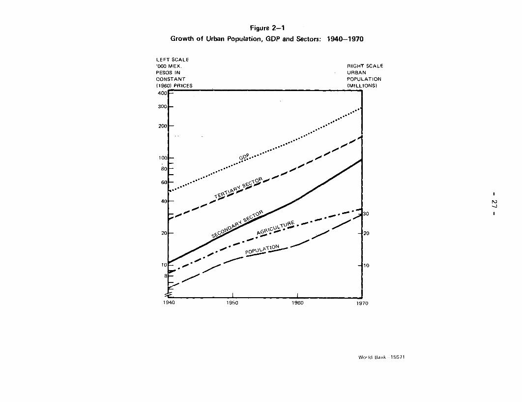
Figure 2-1

Growth of Urban Population, GDP and Sectors: 1940-1970

LEFT SCALE'000 MEX. RIGHT SCALEPESOS IN URBANCONSTANT POPULATION(1960) PRICES (MILLIONS)400 -

300 -

200 - *

100~~~~~~~~~~~~~~~~~~~~~~~~~~~080~~~~~~~~~~~~~~~~~~~~~~~~~~~~00

100 - G9.-'

60~~~~~~~~~~~~~~~0

2C _ _ 0,30

40~~~~~~~~~~~~~~~~~~~1

t _ I ~~~~~~~~I _1940 1950 1960 1970

World Bank-15571

- 28 -

in Mexico was clearly related both to industrializationand developments in the rural sector, but which took placealongside unprecedented population growth.

95. The first correlate of urbanization and economicgrowth derives from the increase in income and the shift ofconsumer preferences towards non-agricultural goods. Whiledemand for foodstuffs becomes increasingly inelastic,demand for manufactured goods and services tends to increase.The demand increases for products which can be most feasiblyproduced in urban agglomerations where scale economies,transfer cost reductions, intersectoral linkages and a widearray of externalities are uniquely available. The cityprovides a "natural" environment for innovation andtechnological progress, whether of original or adaptivenature. Industrialization and urbanization are linked bynecessity and logic, both of which are supported bytheoretical and empirical explanations. Rapid urbanizationin Mexico was a consequence of rapid industrialization after1940. Certainly there is a close historical link betweenthe two (Figure 2.1). The Mexican experience of urban-industrial growth was in many ways synonymous with economicdevelopment as elucidated by Clark (1940) and Kuznets (1958).

96. In the United States and Europe in the nineteenthand earlier twentieth centuries urban-industrial developmentwas characterized by relatively labor-intensive productionmethods in the early stages; the parallel growth of outputand employment in the agricultural sector; and moderatepopulation increase. Urbanization in Mexico in this laterperiod occurred under differing conditions. The economywas unable to absorb the labor force growth arising fromrapid population growth because (1) agricultural outputdid not keep pace with population growth and (2) industrialdevelopment occurred within an environment of capital-intensive technology.

97. The determinants and structure of urban growthare conceived in the development of the secondary andtertiary sectors. The conclusions about the relativeimportance of these factors in determining the courseof urban growth differ significantly from those referringto urban development up to 1940.

- 29 -

B. Transport Development

98. This section describes the development of thetransport system after 1940 and interprets its significancein terms of urban development. We shall examine each modeof transport - rail, road and air - and then analyze theurban implications.

The Railways

99. After 1940 the railway system was shortened (from23,000 km in 1940 to 19,900 km in 1970) while its equipmentand operation were significantly improved. Steam locomotiveswere phased out in favor of diesels, all tracks were! laidto a standard gauge, telecommunication systems were modern-ized and the number of freightcars was increased by morethan 10 percent.

100. The most :important change was the unification,in 1960, of almost all railroad companies (except those ofthe Sonora-Baja California and Southern railroads) into theNational Railroad of Mexico. The new entity became responsiblefor more than 80 percent of the total railnet. Becausedevelopment in the railroad sector after 1940 did not involvethe construction of new lines, there were no significantchanges in the spatial distribution of railroad facilitiescompared with the prior period (Map 4).

101. Freight traffic, which increased at an averagerate of 3.3 percent per annum from 1940 to 1960 and reachedover 9.5 billion tori-km in 1959, was increasingly confinedto bulk (agricultural, mineral and forest) commodities.Passenger traffic increased at 2.3 percent a year and roseto a total of seven billion passengers/km in 1960.

102. The decline in demand for rail freight andpassenger service was closely linked to the development ofhighways and commercial aviation after 1940. The railsystem did not clearly define functions in relation tothese competing modes of transportation.

103. With respect to freight traffic, the status of therailroads was diminished by highway and pipeline development.A 1951 Eximbank survey reported that in all but one instancewhere an all-weather'highway had been built parallel to arail line after 1946, railroad freight traffic had eitherleveled off or diminished the year the highway was put intoservice. During the five-year period 1946-50, railroadfreight activity grew by only 15 percent - a much lowerrate of growth than in the previous five-year period whenfreight traffic had risen by 25 percent.

- 30

104. After 1960, the rail system began to find a newrole. Freight-ton kilometers increased from 13 millionin 1961 to 18 million in 1966. By 1960 the railroadswere carrying more than 20 million ton kilometers a year,but passenger services increased by only 35 percent - from30 million passenger kilometers in 1966 to 46 millionpassenger kilometers in 1971.

105. There are no data on interregional railroad flowsbefore 1970 but the inter-urban origin and destination datafor 1970 (Table 10.7) reveal that railroad movements wererelatively well balanced throughout the country (unlike roador air movements) and that railroad traffic was not dominatedby the major metropolitan centers. In 1970, the entiresystem carried over 49 million tons of freight of which only7.7 percent (3.8 million freight tons) terminated in theFederal District. Monterrey received 1.8 million tons andGuadalajara about .9 million tons (less than 2 percent ofthe national total).

106. The pattern also suggests that by 1970, railroadswere mainly used for the shipment of bulky commodities overlong distances. Most incoming freight to large urban centers,such as the Federal District,originated in remote industrialtowns, or in major ports. 1/ Ten of the 49 cities shown inthe matrix generate more than 77 percent of the total traffic(2.9 million tons out of a total 3.8 million tons).

107. There were heavy flows between medium sizedindustrial cities such a Monclova, Ciudad Obregon, Tampico,Torreon and Toluca, some of which were located close tometropolitan cities and thus served as centers where bulkycommodities were broken down before being transported tothe major metropolitan market.

1/ The Federal District received the largest amounts offreight from Veracruz (about 800,000 tons), NuevoLaredo (about 580,000 tons), Monclova (about 350,000tons), Matamoros (205,000 tons), Ciudad Juarez(135,000 tons), Ciudad Obregon (241,000 tons) andProgreso (175,000 tons).

- 31 -

The Roads

108. During the 1940s and 1950s the largest portions ofroad investment were allocated to new inter-urban roads andto physical improvements (pavement, realignment and safety).The need for improvements in the original trunk system whichwas built in the early thirties arose from the increasedvolume of traffic and the improvement of vehicles after 1950.

109. By the 1950s there were more than 20,000 km of allweather roads in Mexico and road transport services reached92 percent of all urban places. About 15,000 km of the totalnetwork was equipped with two paved lanes and 3,000 km wassurface-treated. Network development generally emphasizedthe trends that already existed featuring new north-southroads from Ciudad Juarez to Mexico City and from Nogalesto Mexico City and a trunk road between Mexico City and theGuatemala border through Tuxtla Gutierrez thereby connectingthe northern and southern borders of the country. Anotherimportant achievement was the completion of a new highwaybetween Villahermosa and Yucatan which connected the capitalwith the southeast. A third development was the Saltillo-Zacatecas route which significantly reduced mileage betweenthese cities and facilitated movement between the threelargest metropolitan centers.

110. In the north, an east-west route was deve]opedfrom Matamoros to Durango, through Reynosa, Monterre!y andTorreon, and was extended to Mazatlan on the Pacific, Coast.In the south, another traverse route across the Isthmus ofTehuantepec was completed in 1960. The three major highwaysfrom Mexico City to the northern border, the principaltraverse roads and many local branch roads followed theroutes of existing railroads,notwithstanding that rationalhighway policy was supposed to stress building roads tolocations which were served inadequately, or not at all,by the railnet. By 1950, consequently, a number of majorcities were still not integrated into the national roadnetwork.

111. Road mileage grew throughout the sixties. In1960, 45,000 km of roads were in service. By 1970, 72,000km of roads were in use (7,000 km were dirt, 20,000 kmtarred, and 42,000 km paved). The road density index ofthe Central region increased from 61.6 km per 1,000 kmin 1960 to 100 km per 1,000 km2 in 1970. The index in thenorth-central and northwest regions for 1970 was five timesabove the national average. The southern region experiencedthe largest gain in the density index (49.9 km per .1,000 km2in 1970 compared to 24.6 km per 1,000 km2 in 1960).

- 32 -

112. Toll roads were introduced in the 1960s in responseto the rapid growth of traffic demand in the metropolitanregion. By 1970 more than 1,000 km of toll roads had beendeveloped in the Mexico City region.

113. The Government continued its efforts to improveinter-regional highway conditions during the 1960s. In1966-73 for example, auto-operation time improved by 10to 25 percent. Major improvements were achieved incorridors to Mexico City (Table 10.14) while transversemovement across the north-central region was significantlyimproved (Tables 10.14 and 10.15). The time-distancevalues show that on the Tijuana-Mexico City road, forexample, operating time decreased by 6 - 12 km/hr, (areduction of about five hours on a bus journey of 45 hours).Driving time on the Mexico City-Ciudad Juarez road decreasedby more than two hours as did that on the road to NuevoLaredo, while driving time between Mexico City and Meridawas reduced from 28 hours 55 minutes in 1960, to 24 hoursin 1970.

Air Transport

114. Of great importance to urban integration in acountry of the size and physical condition of Mexico isthe development of the air transport network which by 1970covered the entire country. The system was serviced by twotrunk carriers (Aeromexico and Mexicana de Aviacion) andseveral feeder lines. 1/

115. In the early 1940s the air transport system wasentirely maintained by private airlines providing servicesbetween Mexico City and other cities. By 1946 five airportshad been built by the Federal Government (Mexico City,Guadalajara, Tijuana, Acapulco and Mazatlan) and eleven byprivate airlines (including those at Merida, Tampico,Monterrey and Nuevo Laredo). However, in order to meet

1/ Most of the feeder lines are under the control ofAeromexico as are the two secondary lines, Aerocarga,S.A. and Servicios Aereos Especiales, S.A. de C.V.(S.A.E.). Aerocarga is destined to become the country'snational air cargo carrier whilst S.A.E., which providessecondary scheduled services within Mexico, is intendedto become the principal Mexican charter line.

- 33 -

the rapid growth of demand and to provide equitableaccessibility throughout the country, the Governmentadopted a civil air transport policy in 1947. Severalnew airports were built in the early 1950s and a numberof major improvement and rehabilitation projects wereimplemented. By 1951 there were 15 airports equipped withnavigation aids, ground support and weather servicefacilities, and some 365 landing fields.

116. Air passenger kilometers increased almost seventimes from 39,000 in 1940 to 308,000 in 1950 and more thandoubled (to 625 million) by 1960 (see Table 10.21). The1960s saw an almost: fourfold additional increase. By 1965,passenger traffic had risen to 2.8 billion p/km. Air cargotraffic also grew rapidly -, from less than half a milliontons in 1960 to over three quarters of a million tons in1965.

117. Since the mid-60s, air transport has become evenmore important, linking urban centers, tourist resorts andindustrial cities. In 1969, more than 4 million passengerswere carried and the number of passenger-kilometers rose toabout 6.8 billion while the average flight length increasedfrom 570 km in 1965 to 840 km in 1969. Cargo traffic exceeded1 billion ton/kilometers in 1969 and has since increased atan annual rate of .10 to 15 percent.

118. The regional and interregional air traffic patternsfor 1967 and 1973 show that in 1967, Mexico City clearlydominated the national pattern, receiving and generatingmore than half of all domestic passengers. Consequently,development of other interregional routes was limited inspite of a well developed schedule of inter-city services.By 1973, the dominance of Mexico City had been somewhatreduced, and a number of important interregional routeswhich did not pass through Mexico City had been developed.Regions outside Central Mexico significantly increeasedscheduled services after 1967, especially in the southeast.

Transport and Urban Development

119. A simple measure of the relationship betweennetwork development and city development was based on acomparative nearest-neighbor analysis of the urban systemin 1940 and 1970.

120. This showed that there was, after 1940, relativelylittle change in the spatial distribution of major cities

- 34 -

(Table 10.28). Between 1900 and 1940 there was a markedchange in this pattern such that, in terms of the largestcities in the urban system in each year, the averagedistances between each major city and its nearest neighborrose from 163 km (1900) to 196 km (1940); the change from1940 to 1970 was only marginal to 202 km.

121. Given the area of the country (1.9 million sq.km) the hypothetical mean distance separating 25 citieswould be 280 km. Thus, in 1900, the actual mean separationdistance was equivalent to only 57 percent of the hypotheticaldistance. By 1940 the percentage had risen to 69.8; by 1970,to 71.9 percent.

122. This suggests that network changes had a muchsmaller impact on the urban system after 1940, and that,notwithstanding the increased efficiency of existing modesand the intensive development of the air network, the majorcities were not brought that much closer to one anotherthan they already had been in 1940.

123. Maps 18-22 show that there has been littledevelopment in relative connectivity between transportmodes after 1940. The major advantage of a location nearthe center of the transport network is the obvious one thatcentrality facilitates access to the rest of the country(see Annex E). This suggests the desirability of locatingcities near the center of the transport network as onemeans of encouraging decentralization.

124. An important indicator of network accessibilityis the frequency or efficiency of service and the conditionsof routes. This is captured by comparing physical with real 1/distances, given that accessibility between two points isnot necessarily a direct function of physical separationand that interregional connectivity does not depend on themere existence of a network link.

125. A recent study (CEPAL, 1974), shows coefficientsbetween real and physical distances. Physical distance wasgiven the value of 1 and was used as a base to which timeand cost elements were added. A value of 1.20 impliesthat real distance is 20 percent greater than physicaldistance, i.e., if physical distance is 100 km the reallength is thus 120 km. Real distances were computedbetween major urban centers along trunk routes or roadjunctions near large cities. Connectivity between regionswas interpreted as connectivity between major urban centers.

1/ See Annex D.

- 35 -

126. Examples of the differences between real andphysical distances are shown below:

Physical RealLength Length Coefficient

1. Acapulco-Mexico City 419 km 611 km 1.46San Luis Potosi-Mexico City 417 km 433 km 1.04

2. Oaxaca-Mexico City 534 km 754 km 1.41Guadalajara-Mexico City 581 km 609 km 1.05

127. In the first example the physical distance betweenAcapulco and Mexico City is virtually the same. When roadcondition variables are taken into account, however, thedistance from Mexico City to each point is very different.The distance to San Luis Potosi is increased by 16 kin, andthat to Acapulco by 192 km. In the second example, althoughin physical terms, Oaxaca is 47 km closer to Mexico Citythan Guadalajara, in terms of real distance it is 145 kmfarther away.

128. Annex E shows that accessibility to the FederalDistrict in terms of physical versus real distance in 1970was excellent to fair in most cases. The Federal Districthad high coefficients with points to the north such asQueretaro, San Luis Potosi, Guanajuato, Pachuca and Leon.There was also excellent accessibility between Guadalajaraand Mexico City (a coefficient of 1.05). Good accessibilityexisted between the Federal District and the northwest (anaverage coefficient of 1.10) and the northeast (an averagecoefficient of 1.09 except in coastal areas). There wasfair accessibility between the Federal District and theSoutheast (coefficients of 1.19 to Veracruz, 1.15 to Merida).Accessibility between the Federal District and the southwestwas only fair (Acapulco 1.46 and Oaxaca 1.41).

129. Monterrey had good to fair accessibility with mostother places. Real distances between Monterrey and suchneighboring towns as Saltillo, Torreon and Nuevo Laredowere moderate and there was fair connectivity with pointsin the northwest such as Ciudad Obregon and Tijuana(coefficients of 1.17 and 1.15 respectively). There waspoor connectivity between Monterrey and Guadalajara (acoefficient of 1.28),which implies that conditions are notfavorable to the formation of strong inter-city flowsbetween these major metropolitan centers. The coefficients

- 36 -

between Monterrey and points south of Guadalajara along thePacific coast were unrecorded but because road conditionswere poor it is assumed that accessibility was low.

130. By comparison with Monterrey and Mexico City,Guadalajara had a lower level of accessibility in termsof real versus physical distance, the coefficients beingconsistently fair to poor except in points to the east -

such as Mexico City which underlies the existence of largetraffic flows between the central region and the Southwest.

131. This clearly emphasizes that differentialtransportation advantages were associated with differentialurban growth and particularly with the growth of the threelargest cities. (See Annex D for information on other cities).The measure of nodal/network relationships further supportsthis conclusion. This concerns relative accessibilitybetween major cities and provides a means of assessing therelationship between changes in relative accessibility andrelative urban development in 1940-70. The analysis isbased on an index of relative accessibility between 25 ofthe cities which dominated the urban system. The use of25 rather than 37 cities is explained by the extremeproximity in 1940 and 1970, of the 37 cities (e.g., MexicoCity and Toluca in macrogeographic terms were in the "same"location).

132. The cities were selected to ensure a minimum of100 km between them and it was assumed that each modeoperated under normal conditions - which implied differentassumptions about average modal speeds and efficiency.Different modal weights were used to reflect qualitativeand quantitative contrasts in transport conditions.

133. The results of the analysis presented in Annex Eshow that the cities with the highest levels of accessibilityin 1940 grew more rapidly than others in 1940-70. Thus,within a general environment in which spatial connectivitywas greatly improved, the places which improved most inrelative as well as absolute terms, were those with thehighest degrees of initial transport advantage at thebeginning of the period. The analysis also showed thatthere was a close relationship between relative accessibilityand relative urban size and urban-economic growth.

- 37 -

C. Industrial Development

134. This section relates the growth and structuralcharacteristics of the industrial sector to the processand structure of urban development after 1940.

General Aspects of the Development and Structure of theIndustrial Sector

135. Industry accounted 1/ for 26.8 percent of GDP in1940 and 34.0 percent, in 1970, with substantial contrastsin sectoral and subsectoral performance from one decade toanother. In general, the manufacturing, construction andpower sectors experienced rapid and sustained growth whilethe mining sector grew less quickly. Industrial expansionwas, over all, faster towards the end of the period thanin earlier years.

136. The expansion of industrial employment wasslower than the rate of growth of output (4.1 percentversus 7.6 percent) and the rate of growth of the urbanlabor force. Economic policies after 1940 generallyimplied that industrial development and diversificationwere considered prerequisites to the achievement of bothrapid economic expansion and the provision of jobs for agrowing population.

137. World War II provided fortuitiously advantageousconditions for industrial growth. Government policiesstimulated industrialization by emphasizing tariffbarriers, import licensing, import substitution and thestrategic allocation of public investment. Infrastructuraland other developments of the 1930s established a basisfor rapid industrialization. By 1940, Mexico was poisedfor "take-off".

138. Although "new and necessary" industries wereclearly defined in successive legislative measures duringthe 1940s, balance of payments difficulties necessit:atedthe introduction of import permits, especially for luxurygoods, in 1947. Thereafter, the proportion of total imports

1/ Includes manufacturing, mining, power and construction.

- 38 -

requiring licenses increased from 28 percent in 1956 to65 percent in 1964. Tariffs were introduced resulting ina gradual increase in the proportion of goods subject totariffs and in the nominal amount of the average tariff.

139. Against this protectionist background, and thegrowth of demand, industrial output increased by 9.4percent a year from 1940 to 1945, the major growth sub-sectors being food, textiles, iron and steel, cement, paperand pulp, and chemicals. Postwar growth was slower, theaverage growth rate from 1940 to the early 1950s beingless than 6.0 percent. After 1950, changing subsectoralemphases were associated with rapid progress in the steel,metal products and chemical subsectors, and with thegeneral expansion of producer rather than consumer goods.

140. The increasing importance of producer goodsindustries is consistent with the pattern described byHoffman (1958), who showed that producer goods tend toaccount for an increasing share of manufacturing productas the manufacturing sector develops. This conclusion isalso supported by the United Nations (1954) in terms ofthe European experience and by Chenery (1960) who foundthat sectoral changes in the composition of manufacturingoutput were associated with rising per capita incomesand increasing national population size.

141. Differential rates of growth and consequentchanges in the subsectoral structure of manufacturing in1940/60 are illustrated in Table 5.2. This shows thatseven subsectors grew at less than the average rate forthe sector as a whole and that as a result, their combinedshare of total manufacturing output fell from more than 75percent of the total in 1940, to less than half in 1960.Among these subsectors, however, food and textiles stillaccounted, in 1960, for more than 50 percent of totalmanufacturing employment and they contributed more thanany other subsectors to the total growth of manufacturing,although their growth rates were below the average for thesector as a whole. Apparel, which ranked fourth in termsof its share of employment in 1960, was also in thiscategory, but nevertheless made the sixth largest contribu-tion to the total increase in manufacturing employment.The only absolute decline was in the machinery subsectoralthough this was explained by a decrease in employment inartisan-type machine shops.

- 39 -

142. The leading growth industries in the 40s and 50swere chemicals, prirnary metals, transport equipment andelectrical equipment, although almost half of the totalgrowth of output in the transport equipment sector camefrom auto repair shops and the data for the 1960s showthat these trends continued through 1970.

143. Table 5.3 uses 1970 industrial census data toshow the percentage distribution of output and employmentby subsector, and indicates that consumer goods accountedfor more than half the total value of output in 1970, andthat foodstuffs and apparel continued to be important interms of employment, while capital and intermediate goodssubsectors continued to be more dynamic.

Industrial Development and Urban Development

(a) Preamble

144. A comprehensive review of the economic rat:ionaleof urban-industrial development after 1940 is beyond thescope of this report. However, some of the general factorsunderlying the relationship between urban and industrialdevelopment - in terms of what may be broadly termedagglomeration economies - have already been mentioned.This section will expand that discussion and complementit with a brief account of other aspects of the urban-industrial link. Market potential, agglomeration economiesand the role of government policies will be discussed, witha brief account of some location factors such as the roleof enterprise, natural resources and regionally specificgovernment programs.

(b) Market Potential

145. There is no absolute proof of the relativeimportance of the market vis-a-vis other factors as adeterminant of urban-industrial growth but it has playeda crucial role in influencing the course of industrial-urban growth since 1940.

146. As noted, apart from the development of "new"producer goods subsectors, the continued growth of consumergoods industries was a major feature of industrial growthafter 1940. For many such industries, the cost of transportof material inputs and of finished goods pointed to a manu-facturing location near the market. The potential size ofthe market for manufactured goods was thus a major locationfactor. This had two aspects: access to population andaccess to incomes.

- 40 -

147. The interstate population distribution in 1940-70is shown in Table 1.9 which emphasizes the continuing dominanceof the Federal District, Jalisco and Veracruz. At the sametime itillustrates the relative increase in the ranks of BajaCalifornia Norte and Chihuahua and the relative decline ofQueretaro. The heaviest increases were in the northern statesand the smallest increases in the south. The contrast wasstronger in 1960-70 than in 1950-60, although the relativegeographic emphasis of growth was the same in both periods.

148. Maps 8 and 9 reflect the consequences of adjustingstate population size to geographic area. In 1940 (Map 8)the rank order of states by absolute size and by densityshows that the Federal District was the highest rankingentity. It also shows that the states of central Mexicohad a generally higher ranking in density than in size,whereas some of the largest states - in both the north andthe south - ranked lower in density than in absolute size.

149. This pattern persisted in 1970 (Map 9), althoughthe density of the southern states had by then notablyincreased, and the high densities of the central stateswere also present in the Gulf states to the east (Veracruz),and in those immediately to the west (Jalisco, Guerrero).

150. In terms of the geographic distribution of demandas measured by population potentials, the center was mostimportant. However, in a country at Mexico's level ofdevelopment it cannot be assumed that the implicit populationpotential (see Technical Annex 9) embodied in the data onpopulation distribution, coincides with that of potentialdemand. The latter is essentially a product of populationweighed by income, and it is therefore necessary to referto certain aspects of spatial contrasts in personal incomelevels and interpersonal income distribution.

151. For certain foodstuffs, purchasing powerdifferentials between rural and urban areas may favorrural families, and to the extent that this is so, theapparent differential between rural and urban incomesshown in Tables 11.2 and 11.3 would be reduced. Stateswith large rural populations are generally unlikely tobe major sources of demand for manufactured goods giventhe low absolute level of rural incomes as well as askewed pattern of distribution.

- 41 -

152. Except in a few states (in the northwest :inparticular), average family incomes in rural areas werelow (Table 11.5). There was a marked difference betweenBaja California Territory where the average rural monthlyincome was Mex $2,317 and Oaxaca, where the average wasonly Mex $376. Clearly, the market potentials of the ruralpopulation of the northwestern states exceeded those ofthe less developed, but densely populated, states of thesouth and center.

153. There were also strong contrasts within the urbansector (Table 11.7). Average monthly incomes ranged fromMex$3,000 in Baja California, the Federal District, SanLuis Potosi and Sinaloa, to Mex$925 in Oaxaca. Thedifference between urban incomes was smaller than thatbetween the highest: and lowest rural incomes. Rural andurban income differentials and the distribution of populationbetween rural and utrban areas account for the pattern ofaverage monthly inc:omes in each state (See Table 11.9). Theweight of urbanizat:ion in the Federal District is reflectedby its income level, the highest of any entity (Mex$3,133),while rural Oaxaca has the lowest (Mex$537).

154. Average income levels multiplied by populationsize are a general referent of market potential. Two otherimportant references are the absolute level of income andthe distribution of income within each entity.

155. Table 11.10 shows broad contrasts in income levelsbetween six major regions and, like Table 11.9, emphasizesthe wealth of the Federal District and the poverty of thesouth and (in general) the center. In absolute terms Table11.11, 11.12, 11.13, 11.14, 11.15 and 11.16 show that theabsolute monthly income of the Federal District greatlyexceeded that of any other region; the central region wasnext highest followed by the south Pacific (more than halfof which came from Jalisco), the north (without particularconcentrations), the Gulf of Mexico (two thirds of which camefrom Veracruz) and the north Pacific (without concentration).

156. The Gini coefficients in Table 13.18 show thedistribution of the average level of income in each state.There is a high (.78) coefficient of correlation whichsuggests that the states in which personal incomes in1969 were highest were those with the most equitablepatterns of distribution. At the extremes, the FederalDistrict had the highest level of income (Mex$628) andthe fifth lowest Gini coefficient (.501) while Oaxacahad the lowest level of income (Mex$109) and the highestGini coefficient (.688).

- 42 -

157. The conjunction of relatively high averageincomes and a pattern of relatively good income distributionin the center, the northwest and the north, points to arational location for market oriented manufacturingactivities in these areas. In particular, manufacturinggrowth in Mexico City was closely related to its hugeinternal market which gave rise to considerable agglomerationeconomies in both the District and in contiguous parts ofthe State of Mexico. By 1960 only two cities - Monterreyand Guadalajara - had surpassed Mexico City's populationin 1900 (344,721). This indicates the tremendous advantageaccruing to the capital from its market size, an advantagewhich was also reflected in its share of retail sales(Table 9.3).

158. Interstate contrasts in income potential werecoupled with the relative advantages and disadvantagesderived from the structure of the transport system (alreadydiscussed from a general point of view) to provide acontrasting pattern of market opportunities for differentcities. The significance of network accessibility derivesfrom the lack of sufficiently large aggregate populationsand incomes to achieve scale thresholds basedexclusivelyor even primarily on internal demand for other thanessential consumer goods. In serving a regional marketof a given size, manufacturers in poorly connected citieshave longer shipping distance and higher transport coststhan those in well connected cities.

159. By 1940, there was already a coincidence betweenaccessibility to markets and network structure. For reasonsof resource base development or agglomeration, transportimprovements had already conferred a lasting pattern ofrelative advantage and disadvantage with respect to industrialgrowth in cities. In 1940, a number of cities with relativelylow levels of accessibility in terms of market potentialhad relatively high connectivity as measured by transportand communications networks. Some of these cities weresmall in 1940 but managed to grow rapidly in 1940-70. Itcan be argued that they did so despite limited marketpotential, but they could not have done so without anadvantageous situation of connectivity.

- 43 -

(c) Agglomeraition Economies

160. Agglomeration economies derive from the increasein internal and exlernal economies accompanying the spatialconcentration of population and economic activity. Thereare several kinds. The first concern plant size and areinternal to the firm. Coefficients for three alternativemeasures of plant scale in manufacturing - capital invest-ment per plant, employees per plant, and output per plant -show that average plant size was greater in the more developedstates (Table 7.14) and in larger cities. The increase incoefficients for emnployees per plant and output per plantbetween 1940 and 1970 suggests that these scale differencesmay have become sharper over the thirty-year interval becausemanufacturing plants in larger cities probably benefittedmore from internal economies of scale than others duringthe period.

161. Manufacturing growth has been fastest in citieswhere industry was able to make the greatest strides inincreasing plant sizes, average plant size (measured byoutput per plant as a percent of the national average)being generally higher in those states which experiencedrapid growth in manufacturing employment and output.During the "Porfiriato", manufacturing growth and scalechanges were not, in general, closely associated withdifferential rates of urban growth.

162. A second class of agglomeration economies areexternal to the firm. Among them, the supply of labor andcapital appear to have been particularly significant.

163. Skilled labor was a more crucial determinant ofindustrial location than the aggregate supply of labor 1/.This is consistent with a high level of marginal employmentin both the urban and rural sectors and with migrat:oryfactors that tend to mitigate interregional differences inlabor supply. Capital and unskilled labor must, in general,be combined with minimum amounts of skilled labor to determine

1/ Skilled workers are "those who, as a result of theoreticaltraining or considerable experience, are capable ofrealizing a complex and specialized task and whose servicesare contracted precisely for that purpose", VII CensoIndustrial, 1961, p. SVII.

- 44 -

the effective overall supply of labor manufacturing. Thus,a predictably strong relationship exists between theproportion of skilled workers to total workers in manufacturingand the incidence of urban/industrial growth both at thestate and the city level.

164. In the integrated economy, which evolved in Mexicoafter 1940, the local availability of capital is not necessarilyan important determinant of industrial location. However,Myrdal (1957) argues that in the early stages of economicdevelopment, the expanding scope for external economies inhigh growth regions will raise profits and income levelswhich, in turn, will lead to higher rates of savings.Increased savings are then invested, which further expandsthe scope for external economies. Hirschman (1962) supportsthe argument that savings, as well as investment, tend to behigher in growth poles experiencing agglomeration economiesand both contend that advancing regions tend to securerelatively larger shares of government investment.

165. The interstate distribution of private savings percapita in 1940 and subsequent increase were consistent withhigh differentials in rates of private savings between moreand less developed states and those in which manufacturingdevelopment was relatively advanced or retarded (Table 3.6).This pattern continued in later years. In 1970, the patternof savings emphasized the dominance of the Federal Districteven more than in 1940; by that time almost half of the totalbank deposits were concentrated there despite a marginaldecline in dominance since 1960 which might indicate thebeginning of a new pattern of savings.

166. Disparities in private credit appear similar tospatial disparities in private savings (Table 3.7). Thedominance of the Federal District in private credit waseven greater than in savings in that it accounted in 1940for more than two-thirds of total credit for the wholecountry. Other areas or relative credit concentration atthat time were Nuevo Leon, Coahuila, Sinaloa and Sonora.By 1970, the dominance of the Federal District was evenstronger. Nuevo Leon, Chihuahua and Jalisco followed interms of aggregate credit allocations.

167. There is no available data on the sectoralallocation of either private or official credit prior to1965. In that year industrial credit accounted for almosthalf of total private credit, with most of it allocated tocommercial activities (Table 3.8). In both respects, theFederal District was strongly dominant. With respect to

- 45 -

the smaller volume of total official credit, the sectoraland geographic distribution was roughly similar to that ofprivate credit, although the Federal District had a nearmonopoly on official credit for industry. The pattern in1972 (Table 6) was roughly comparable, although the shareof the Federal District in private industrial credit hadby then somewhat declined.

168. Clearly manufacturing development and urbanizationwere strongly associated with the accumulation of savingsand relatively high levels of investment. Indices of invest-ment in manufacturing and agriculture support the hypothesisthat rates of private investment were highest in the mostdeveloped states and in the largest and most dynamic cities,suggesting, inter alia, that industrial capital was notgenerally as horizontally mobile up to 1970 as might havebeen expected.

169. A third class of agglomeration economies are alsoexternal to the firm and comprise a variety of intersectorallinkages. First, the concentration of commercial and servicefunctions in large cities implies that large cities offerthe manufacturer greater relative advantages than smallercities. In particular, the role of Mexico City as thefinancial and commercial center of the nation was stronglyassociated with its growth as a manufacturing center.Access to financial and other specialized services wasalso an important variable in investment decisions.Derossi (1972) points out that access to Government serviceswas particularly crucial, even for entrepreneurs with firmslocated in Monterrey, and that it is not uncommon to findthat large enterprises located in other cities maintainpermanent offices in the capital. 1/

170. Second, good access to coal and ore deposits werevery important to the expansion of the basic metals industryin Coahuila and Nuevo Leon, but these raw materials were notlocated in the State of Mexico and the Federal District. Bothstates experienced substantial development in this sector,which can be mainly ascribed to the effects of transfereconomies arising from relatively low freight rates on rawmaterials. In all four states, the concentration of basic

1/ In at least one instance (no doubt there are others),a firm which has its only plant in Monterrey has itshead office in Mexico City, 600 miles away.

- 46 -

metals stimulated growth in the forward-linked fabricatedmetals, transportation products, and electrical machineryand apparatus industries. In turn, the automobile assemblyindustry, located in the Federal District and the State ofMexico, gave impetus to the backward-linked rubber tireindustry in these states. The resulting large concentrationof industrial demand (except in Coahuila) also promoted theproduction of intermediate goods, such as synthetic fibres,industrial acids, cement blocks, and glassware; while theaccompanying concentration of consumer demand, resultingfrom a large labor force, stimulated the output ofpharmaceuticals, processed food, and other consumer goods.

171. Transfer economies derived from the adjacentlocation of closely-linked industries and from internaleconomies of scale created by the spatial concentrationof large industrial and consumer markets. The earlyprominence of Mexico City and Monterrey, as populationand manufacturing centers, placed them in a particularlyadvantageous position to attract the new large scaleindustries which the economy was able to support after1940. Conversely, where industrial growth was based onaccess to primary materials in rather small urban areas(Monclova for example) 1/ consumer and other intermediategoods industries (e.g., textiles and chemicals) did notgrow rapidly.

(d) The Role of the Public Sector

172. Government policy in the evolution of the spatialstructure of the industrial sector after 1940 revolves aroundtwo issues. First, macro-economic policies, which had animportant effect on spatial and urban development but inwhich there was no formal spatial dimension. Second, policieswhich had an explicit spatial dimension and which weredesignated as such, or if not, can be recognized as, atleast in part, deliberately spatial policies.

1/ Monclova was not one of 1970s largest cities.

- 47 -

(i) The Urban Impact of General Economic Policiesfor Industrial Development

173. The most important policy in this category (andthe only one which will be discussed here) concerns externalprotection. As noted earlier, Mexico's industrializationafter 1940 was closely associated with import controLs andtariff barriers with emphasis on the former. Compared withother Latin American countries, Mexican industry is notunduly protected, but this strategy has affected the spatialstructure of the industrial sector.

174. Import substitution, which began in the 1940s, ledto certain inefficiencies in industrial development. Highproduction costs were associated with the fragmentation ofmuch of Mexico's industry into small firms, often usingbackward techniques of production and management. They werealso related to inadequate specialization within the manu-facturing sector because the system of import licensingencouraged backward integration with firms producing variousparts and components for their own use rather than buyingfrom domestic suppliers.

175. Protection hindered efficiency because firms wereassured of high profits in a closed domestic market. Thus,technical progress was slow and the quality of many manu-factured goods, poor. The low quality of industrial, inputsalso adversely affected commodities at higher levels offabrication. Import substitution behind protective barriersled to the establishment of industries (mainly capital-intensive) in which Mexico had little comparative advantage.The mechanics of protection emphasized quantitative controlsrather than tariffs, with the benefits going almost entirelyto the private rather than the public sector, resulting ina regressive impact on income distribution.

176. Lavell (1972) has analyzed the spatial impact ofprotection with specific reference to the Law of New andNecessary Industries introduced in 1941 and amended in 1946and in 1955. Industries covered by the Law included: basicmetals, transport, chemical, mechanical, electrical, metaland food products. The law grants total relief from excessprofits, stamp, industrial and income taxes and from importduties on raw materials or components needed in production.

177. Exemptions were granted for periods of five,seven or ten years depending on the industry and its relativeimportance for national development. "New" industriesincluded branches of manufacturing which were not well

- 48 -

represented in Mexico and those producing a similar productto one already produced in a national plant, provided thatthe new company guaranteed a 20 percent saving in the priceor the lifespan of the new product. "Necessary" industrywas defined as that which was of fundamental importance tothe nation's industrial growth.

178. The law had no explicit spatial dimension. AsNavarrete (1967) correctly emphasized, the Federal Governmentgranted identical exemptions throughout the country, withoutreference to spatial, regional or urban development. Inpractice, however, most of the exempt firms were locatedin the Valley of Mexico and at least 65 percent of thecapital investment and 40 percent of the employment linkedwith the law was in or around Mexico City. By 1960, 19of the 32 states had not received a single exemption. By1965 the number had been reduced to 15.

179. Table 6.6 shows the regional distribution ofexemptions in three periods; the heavy concentration in theCentral Region and to a lesser extent in the northwest areclearly apparent. Table 6.7 emphasizes the same point, butmore strongly, because it can be inferred that 98 of the167 plants established under the Law in 1959-64 were in ornear Mexico City, and 21 were in Monterrey. Table 6.7 showsthe sectoral incidence as well as the geographic distributionof the exemptions.

180. The absence of a spatial dimension in the law andin the policy of protection in general, does not thereforeimply that it had no spatial effect. The lack of a spatialcomponent is attributed to the government's concern to promotenational industrial development. When the law went intoeffect, some parts of the country were severely disadvantagedcompared to others. In terms of infrastructure and accessibil-ity, to have encouraged location in the periphery would havebeen inefficient because already inefficient producers wouldhave had to contend with cost disadvantages attributable tolocation. But, if the law had included a spatial objective,the response of entrepreneurs would have been less enthusiasticand Mexico would have experienced less real growth than itdid. Nonetheless, external protection and industrial central-ization were closely related phenomena.

- 49 -

(ii) The Spatial Impact of Industrial Policieswith Explicit Spatial Dimensions

181. Among the policies in this category are (1) fiscalpolicies - which were developed by the states; (2) creditpolicies which were developed by the Federal Government; (3)public investment policies; and (4) wage, price and tariffpolicies.

- Fiscal Policies

182. Between 1940 and 1960, almost all of the statesintroduced tax exemption laws to encourage industrial develop-ment. These laws allowed for exemptions from the state'sshare in the sales tax, from stamp duty, and from local landtaxes and were applicable to both new and expanding industries.Exemptions varied from 10 to 30 years, depending on the stateconcerned.

183. Romero Kolbeck and Urquidi (1952) concluded thatthe effects of exemptions on industrial development in theFederal District had served little useful purpose and hadresulted in an unnecessary loss of fiscal revenue. Theyalso argued that the objectives of tax exemption were, inthe case of the Federal District, dubious because there wasalready an excessive concentration of industry in the area.They added that if exemptions were to be continued, theyshould only apply to industries which would "lead to animprovement in the standard of living of the population."Finally, they proposed that if exemptions were to becancelled for 61 percent of the factories studied, thecancellation of exemptions would lead to a 10 percentloss in profits and for 14.9 percent of them, a 25 percentloss. If passed on to the consumer, this would imply anincrease in prices of only 1 or 2 percent a year. Not longafter the publication of their study, tax exemptions wereabolished in the Federal District.

184. It has been argued that essentially similarexemption laws had a countervailing impact on industrialgrowth in other parts of Mexico and, to the extent thatexemption was used, a loss of fiscal revenue ensued. More-over, on the basis of somewhat scanty empirical evidence,the laws did not produce a positive effect on locationdecisions. Lavell (1972) reports that very few, if any,of a group of entrepreneurs in the states of Puebla,Guanajuato, Queretaro and Cuernavaca accorded muchsignificance to the exemption laws.

- 50 -

- Credit Policies

185. In 1953, the Guarantee and Development Fund forSmall and Medium Industry was used as an explicit instrumentof industrial location policy. By 1960, the industriescovered by the Fund accounted for 57 percent of all industrialplants in Mexico and for 79 percent of industrial employment.By June 1970, the Fund had awarded some 10,000 credits tomore than 5,200 firms; the credits represented 32 percentof total capital investment in the companies concerned, whichemployed a total of 187,000 workers. The spatial strategyof the Fund was to "attempt" to select factories locatedoutside the areas of industrial concentration. Table 6.8shows the regional distribution of credits granted between1953 and 1970. It shows that, over time, the relativeimportance of Jalisco, Mexico and Sinaloa increased, butthe average size of credits in the Federal District andthe State of Mexico was relatively large throughout theperiod.

186. Table 6.9 confirms that marginally the share ofthe Federal District decreased. In 1961-62 it attracted48 percent of all credits granted, whereas in 1969-70 itattracted only 23 percent. However, the marginal participa-tion of the State of Mexico increased over time. The dataindicate that, given the rising shares of Jalisco, Sinaloa,Sonora, Guanjuato and Oaxaca in the numbers of creditsgranted, the policy was a small step towards the spatialobjective of decentralization.

187. The limited flows of credits to provincial areasmay have been related to the lack of knowledge about creditfacilities outside the central core and a few other regions.Lavell (1972) finds it difficult to believe that during thelast 15 years, the economies of Zacatecas, Campeche, Colima,Nayarit and Tabasco could only support a demand for 10 orfewer factories requiring credits. The Fund took specificnotice of this problem in trying to publicize its existenceto less developed states.

- Public Investment

188. The direct relationship between the spatialallocation of public investment and that of industrial growthconcerns the allocation of public investment to the industrialsector. Prior to 1959 there are no data on the geographicdistribution of public expenditure. From 1959 through 1970there are detailed data on outlays in each state by sector.

* 51 -

The industrial sector accounted for 8 to 15 percent of totalpublic investment in this period, about 80 percent of whichwas in the hydrocarbons sector. Industrial investments werehighly localized and Tamaulipas and Veracruz accounted forsome 60 percent of hydrocarbons investments while steelinvestments were heavily concentrated in Coahuila.

189. The indirect relationship between the spatialstructure of industrial growth and that of public investmentwas more important than the direct relationship, becausegeographic differences determined the availability oftransport facilities, power, water and other goods andservices which, in one way or another, had a bearing onthe attractiveness, and even the viability, of alternativelocations for industry.

190. In the period for which consistent data are avail-able (1959-70) the geographic allocation of public investments,in sectors other than industry and agriculture, shows thatthe Federal District received the largest share of totaloutlays throughout the period, although the share has declinedsomewhat in recent years (Table 3.16). The geographicdistribution of infrastructural investments of all kinds(transport, power, water) was found to be closely relatedto the incidence of urbanization at the interstate level.There was a similarly high degree of correlation betweenurbanization and public investment in education, the FederalDistrict again receiving a disproportionately high share(with respect to its share of the nation's population) oftotal outlays in these sectors. The Federal District. alsoaccounted for an even larger share of total investment inadministration because of its role as the seat of theFederal Government, although this category of expenditurewas less important than others.

- Wage, Price and Tariff Policies

191. Since 1946, minimum wages in Mexico have been setby a tripartite commission and appearances might suggest,given that wages were consistently lower outside the largestmetropolitan areas ard the northern frontier (see be:Low)that wage differentials encouraged industrial growth inperipheral areas. However, minimum wages were mainlydesigned to take account of cost of living differentialsand there is little evidence that geographic differencesreflected anything more than this. It is difficult tofind evidence that wage policy was ever used in a consciouseffort to promote industrial growth in the periphery.

- 52 -

192. With respect to public sector prices and tariffs,general evidence shows that government policies did notencourage decentralization. In the Federal District, waterprices were held down so that consumers paid less than theincremental cost of bringing water to them. Prices of corn,electric power, diesel fuel and public transport were alsosubsidized in the Federal District from 1940-70. Althoughsome of these policies were to benefit the urban poor,substantial parts of the subsidies benefitted other groupsand inevitably reduced the costs of locating economicactivity in the Federal District, thereby creating adisincentive to locate elsewhere.

193. As argued earlier, progress in transportation wasa positive factor in facilitating decentralization after1940. However, two issues deserve attention here. First,rail freight rates were structured to favor transport routesbetween Mexico City and other points over other routes.Second, the basis of rate-making was "value of service"and this tended to increase the costs of transporting bulkcommodities. The effect of this pattern of cross subsidiza-tion was to encourage location near markets rather than nearraw materials, and thus to favor the core rather than theperiphery. Finally, property in the Federal District wasrelatively under-valued for tax purposes. Other statestaxed at higher rates because local taxation was necessaryto finance public education, whereas education was financedby the Federal Government in the Federal District. This tooreduced the relative costs of locating in the Federal District.

(e) Other Determinants

194. Other circumstances--some of general (but minor)relevance, others of local (but great) importance--affectedthe process of urban-industrial development. A completereview of these factors other than those included in thethree broad categories we have so far considered is impossible.But a selective review, focussing on locally relevant factorsis not only feasible but important because the evidencesuggests that such factors may, at this level, have outweighedthe more general conditions we have already discussed.

195. The first such factor concerns the decision-maker.Industrial location decisions are necessarily made by peoplewith varying abilities to make rational choices and who mayor may not be well informed when taking the decision.Entrepreneurs (or industrial decision-makers) may vary inwillingness to take risks, etc. Contrasts between

- 53 -

entrepreneurial groups may have an important bearing- onindustrial development. The available data suggest thatsuch contrasts in Mexico are specific to cities ratherthan to states or regions.

196. An exhaustive review of this topic is beyond thescope of this report. The general significance of enterpriseas a location factor can be illustrated by reference to theexample of Monterrey. Derossi (1971) has shown that: by 1940the effect of antecedent industrial development had alreadyestablished this city as a leading industrial center andthat its growth after 1940 was, to a large extent, based onthe continued exploitation of its initial advantage vis-a-visother cities and regions. Even so, the continued ability ofMonterrey to compete successfully with other cities after1940, in spite of its peripheral location relative to thecentral market, depended upon the ability of its entrepreneursto identify and develop new opportunities for expansion.There may be a parallel here between the role of en-terprisein Monterrey (and, by extension, Nuevo Leon), and in Medellin(and, by extension, Antioquia), Colombia. 1/ Certainly thereis some evidence that the entrepreneurs of Monterrey likethose of Medellin have sought new opportunities not onlyin situ but also in other parts of the country.

197. Another relatively localized determinant of urban-industrial growth after 1940 concerned natural resources.In earlier periods (see Chapter 1) we found that these playeda crucial role in industrial development. After 1940, theirimportance appears to have been local rather than general andcan best be illustrated by reference to the experience ofthe northern states of Chihuahua, Sonora, Tamaulipas, Morelos,and Baja California Norte, where raw material processingindustries (most of which produced for export to nationalor international markets rather than for the local market)provided the main source of manufacturing expansion..

198. Cotton ginning and weaving utilized part of thelarge amount of raw cotton grown in these states, while theoil extracted from cotton and other oil seeds was importantfor industrial inputs. Cattle raising stimulated the meat

1/ See Hagen (1965). San Pedro Sula, Honduras; SantaCruz, Bolivia;and in a somewhat different way, SaoPaulo, Brazil might also fall into the same cat:egory.

- 54 -

packing industry in the city of Chihuahua while the wheatand rice milling industries processed the large quantitiesof wheat and small quantities of rice produced in thenorthern states. Beerproduction, based on local grains,achieved prominence in Tijuana and Mexicali and petroleumrefining gave a significant impetus to industrial expansionin Tampico. Favorable access to raw materials inputs, andexternal demand for the products of these industries,stimulated heavy capital investment and the establishmentof relatively large-scale plants in the northern cities.The expansion of these industries also seems to have inducedsecondary growth (via multiplier effects) in the vehicles,tires and tubes, and electrical apparatus industries; inthe lime, plaster and stone industries providing constructionmaterials from local mineral inputs; and in some localconsumption goods industries, such as beverages and printing.Other growth stemmed from insecticide and fertilizer industriesproviding inputs for the agricultural sector, which in turnfurnished raw materials to some of the major. growth industries.

199. The final example of a "local" factor which had adirect and important bearing on urban-industrial growth after1940 concerns the impact of a regionally specific governmentpolicy: the "assembly industry" or maquila program of thenorthern (U.S.) border, which was started in the 1960s.

200. The border region stands apart from the rest ofthe country. Its trade and cultural relations are largelywith the U.S.,and the high levels of immigration to theregion after 1940 were closely linked to the possibilityof obtaining employment in the United States. From the1940s the development of the "Bracero" program, whichfacilitated the temporary migration of Mexicans to workin farms across the frontier, provided an important sourceof employment. By 1964, it employed nearly 200,000 workers.In 1965 the U.S. Government terminated the program, andthe Mexican government initiated the Border IndustriesProgram to facilitate sub-contracting by U.S. industrialfirms, taking advantage of the availability of inexpensivewage labor in the Mexican border states. 1/

1/ Articles 806.30 and 807 of the U.S. Tariff Scheduleprovide that imported products assembled in foreigncountries with components made in the U.S. are subjectto customs duty only on the basis of value added abroad.

- 55 -

201. The program was launched with multiple objectives.These included: the growth of employment; the generation offoreign exchange; the upgrading of the labor force; wideningthe domestic market for Mexican producers by injecting incomeinto the region; increasing fiscal revenues; stimulatingmultiplier activity in non-manufacturing sectors and expand-ing the market for skilled Mexican labor.

202. The legislation introduced in 1965 was such thatthe so-called "maquila" industries located in the BajaCalifornia and Sonora Free Zone were governed by regulationswhich differed from those applicable to other border areas.They were allowed to import any item included in the FreeZone Import List, whereas plants located in other borderareas had to obtain "temporary import" permits for theirspecific required inputs. The initial temporary importpermit for new "macuila" industries in the border areasbut outside the Free Zone had to be sanctioned by theMinistry of Industry and Commerce and the Ministry ofFinance in Mexico City. Repeater permits were granted bya local committee in the concerned border area. Theseadministrative arrangements worked fairly smoothly, andborder area industries of both kinds considered themselvesadvantageously placed compared with plants in the interiorwhich also required temporary import permits.

203. The major "maquila" industries, whether locatedin the Free Zone or in other border areas, were subsidiariesof US corporations. The latter provided capital, physicalinputs, and often management and guaranteed to purchase theentire output. The terms under which the Government allowedthem to be established required them to declare costs andrevenues and to pay Federal and State taxes on sales andprofits. But these conditions were generally bypassed--particularly by foreign-owned companies. Many foreignfirms did not keep financial data or accounts in theirMexican plants and received inputs of nominal value andtransferred their output at or near the domestic costincurred in Mexico. Hence the "value" of exports declaredto government authorities was often an approximation ofdomestic value added. This position was clearly verydifferent from that of Mexican firms located in the interior,which imported inputs on "temporary" licenses for processingor assembly into export products. Mexican firms in theborder areas appeared' to be in a somewhat ambiguous position,depending on the discretion of local officials.

- 56 -

204. There can be no doubt that the program had adramatic impact, both on the frontier region and on Mexico'smanufactured exports. It is, however, unreasonable to claimthat it has been fully successful even with respect to itsstated objectives. Analysis of the consequences of the growthof the border industry program suggests that it may haveproduced some undesirable effects.

205. Its quantifiable impact on the local, regional andnational economy cannot be determined with great precision,but it is estimated that by the early 1970s, the program hadgenerated some 50,000 jobs, mainly for women in the agegroups 15-24. Minimum wages in the border area had longbeen higher than elsewhere, and rose quickly after 1966.By 1972 they ranged from an average of Mex$21,000 per yearin Nogales to Mex$14,400 in Laredo and Matamoros. However,while employers in the interior, and especially in theFederal District, have to incur considerable expenses onfringe benefits, border industries generally pay only theminimum prescribed wage. The difference in total cost perunit of labor is not so great as that shown in publishedminimum wage schedules. It seems likely that there iswidespread use of on-the-job trainees by border plants, apractice which may point to the exploitation of Mexicanlabor laws.

206. Foreign exchange earnings disaggregated intogross and net exports originating in assembly plants arenot available prior to 1970. On the basis of the growthof employment, foreign exchange earnings before 1970 werelower than might be expected. It is estimated that 70percent or more of the wages earned by Mexican employeesis spent in the U.S., representing an enourmous "leakage"and indicating the failure of the program to widen themarket for Mexican producers, largely because of theinfluence of U.S. consumption patterns in the border cities.

207. From a fiscal standpoint, the results have beenpoor. If the U.S.-owned firms in the border areas were tocomply fully with the basic terms of the regulations andto declare the full value of their inputs and outputs, theGovernment of Mexico would gain in the collection of bothsales and income taxes. Parent firms in the U.S. would notsuffer from paying Mexican income taxes on their subsidiariesbecause of the U.S. provision of credit for foreign tax pay-ments. The sales tax payments would, however, represent anadditional cost.

- 57 -

208. Finally, it is unlikely that the program has hadthe intended results with respect to labor force skcills.

209. The most serious "failure" of the border industryprogram is that it has not reduced the traditional dependencyof the region on the U.S.A. There is still a mass:ive"leakage" of resources across the frontier. Although theprogram has generated more income in the area, much of itis "lost". As a result, the border cities remain enclaveeconomies which are essentially disarticulated from therest of Mexico. This judgment may seem harsh in view ofthe apparent success of the program in certain respects.Yet, if spatial development implies the generation of"spread" effects within the national economy, the resultsof the program through 1970 did not achieve this.

D. Tertiary Sector Development

210. While profitability may be regarded as a generaltest of the relative viability and attractiveness of.alternative locations for tertiary activities, there arecertain contrasts with the secondary sector and thereare also important differences between one tertiary industryand another. Commerce and urban services are dependenton market potential within the framework of a functionalhierarchy of central-place activities. Tourism, however,has very little relationship to demand originating in anurban or even a regional market and is, to a very largeextent, related to international demand.

211. There are few cities in which initial tertiarymultipliers seem to have played a decisive role. Tro someextent, services, especially government, were crucialsectors in Mexico City, in the sense that its initial size(in 1900) was in many ways a consequence of its historicaldevelopment as an administrative and political center. Butthe major instances where tertiary functions played a decisiverole in generating urban growth were those of the bordercities of Tijuana, Mexicali, Ciudad Juarez, Reynosa, NuevoLaredo, and Matamoros plus the major tourism centers ofAcapulco and Mazatlan on the Pacific Coast.

212. The key to growth of the border cities is thelarge market potential--not in Mexico, but in the USA.After 1940, the development of new industrial productionfor the US market became a major cause of expansion, andin the late 1960s the border industrialization programalso became import:ant. The development of a cluster of

- 58 -

entertainment and recreation industries in Tijuana and inother border cities was a major force in the growth oftheir populations and economies.

213. With respect to growth based on tourism, thephysical attributes of the Pacific Coast were clearlyparamount in determining sectoral development in Acapulcoand less markedly, in Mazatlan. Both enjoy remarkablenatural settings and this was the primary force ingenerating growth after 1940. Clearly, it requiredenterprise and enthusiasm to exploit these resources. Butgrowth was essentially based on an initial developmentimpulse from new investment in non-industrial activityand corresponded to an export-base development model.Normally an export-base is associated with the growth ofsecondary sector activities, but here is a case in whichit was linked with tertiary development, the multipliereffects of which led to the subsequent growth of industrialand tertiary activities.

3. THE SOCIO-ECONOMIC STRUCTURE OFTHE URBAN SYSTEM, 1940/70

A. The Demographic Structure of the Urban System

The Demographic Characteristics of the System

214. The structural development of the urban systemis based on a set of cities which constituted the upperlevel of the urban hierarchy in 1970, as conceived in termsof a population of about 100,000. Thirty-seven cities fallinto this category, the largest being Mexico City (8,500,000)and the smallest Pachuca (92,000). The population of eachin 1940, 1950, 1960, and 1970 is shown in Table 1.23. Theirrelative sizes are shown in Table 1.24 and (in size cohortform) in Table 1.27.

215. The population growth rates are shown in Table1.28. The highest growth rates in 1940/50 were those ofTijuana (11.5 percent), Mexicali (10.9 percent) and Reynosa(10.6 percent). The fastest rates in 1950/60 were those ofTijuana (9.7 percent), Mexicali (8.5 percent) and Hermosillo(8.1 percent). In the final decade of the period (1960/70)when urban growth was generally slower, the fastest growthrate was in Acapulco (10.9 percent).

- 59 -

216. During the period of 1940-70, four cities -Tijuana, Acapulco, Mexicali and Ciudad Juarez - grew atan average annual rate exceeding 7.0 percent; five othercities sustained an average growth rate of more than 6.0percent; and five more grew at an average annual rate ofmore than 5.0 percent. There was, in general, no relation-ship between relative population size at the beginning ofthe period (1940), and subsequent population growth, whichimplies that initial advantage in population terms was nota crucial determinant of differential urban size growth.

217. The growth pattern in each city shows contrastscompared with the average rate of growth for all 37 cities(Table 1.29). Some cities (e.g., Culiacan, Minatitlan andJalapa) grew faster than the average rate in one decade andmore slowly in another; some cities (e.g., Guadalajara,Tijuana and Mexico City) sustained a faster than averagegrowth rate throughout the 30-year period, and some (e.g.,Aguascalientes, Morelia and Orizaba) grew at a less thanaverage rate in each of the three decades after 1940.

218. The trend of increasing urbanization was associatedwith an increasing concentration of the urban population inthe 37 cities which dominated the urban system in 1970 (SeeTable 1.55). Within this framework there was furtherconcentration in the ten largest and five largest citiesand in Mexico City (See Table 1.54). The 37 largest citiesaccounted for 65.0 percent of the nation's urban populationin 1940 and 68.0 percent in 1970; the ten largest cities,for 46.0 percent in 1940 and 50.0 percent in 1960; the fivelargest cities, for 38.0 percent in 1940 and 43.0 percentin 1960 and Mexico City, for 26.0 percent in 1940 and 30.0percent in 1960.

219. Up to 1950 increasing urbanization was associatedwith increasing primacy (i.e., an increasing proportion ofthe total population of the largest cities was concentratedin Mexico City). In terms of the 25 largest cities therewas a continuous increase between 1940 and 1950 in the ratioof the size of Mexico City to the total population of thecities occupying the second through the 25th ranks in theurban hierarchy (i.e., the rank order of cities). After1950, however, there was a decline in the ratio between thesize of Mexico City and the size of the second ranked city(Guadalajara) and also in the ratios between the size ofMexico City and the cities occupying the third through thetenth ranks. These contrasts imply that the maximum degreeof primacy in the urban system was reached in the ]940s andthat thereafter, the country's major regional centers becamerelatively more dynamic than Mexico City. As a result of thefirst implication, the "balance" of the urban system wasgradually improved after 1950.

- 60 -

220. We also find that the urban system became increasinglystable over time. Analysis shows (Table 1.43) that the member-ship of the sets of the five, ten, and 25 largest cities in1940/70 was remarkably consistent, suggesting that once estab-lished in the upper limits of the urban hierarchy, citiesgenerally grew fast enough to remain there. This conclusionis reinforced by rank-order correlation analysis (Table 1.45)which shows that the stability of the order of urban systemwas very high throughout the period of 1940/70, even interms of the 25 largest cities.

221. These findings suggest that the urban system becameincreasingly "mature" after 1950 but this is not supportedby the results of a rank-size rule analysis (Tables 1.47 to1.50). It is frequently assessed that a "mature" urban systemis characterized by a harmonic lognormal progression. Analysisshows more deviation from a rank-size structure in 1970 thanin 1940 and that the discordance was greater in the tenlargest and five largest cities than in the 25 largest cities.The degree of discordance increased from one decade to thenext. The structure, however, is severely distorted by theabsolute size of large cities, such as Mexico City.

The Origins of Urban Growth

222. There were marked differences in the relativeimportance of natural increase and migration as sources ofpopulation growth in the nation's largest cities. The periodof fastest urbanization - from 1940 to 1950 - was marked bya massive growth of rural-urban migration in the 1940s, anddiminution thereafter, and by the trend of acceleratingnatural increase after 1950. Thus the growth of large citiesin the 1940s was mainly the result of migration. In the1950s and 1960s, the growth was primarily due to naturalincrease, although the absolute numbers of migrants continuedto rise.

223. In addition to migration and natural increase, athird, and only locally important factor in accounting forurban population growth, was the process of accretionwhereby cities expanded, and in so doing, incorporatedexisting and formerly separate rural communities. Thisprocess was significant in the densely populated centralregion and was particularly important in the case of MexicoCity, where urban size growth and the outward extensionof the city towards formerly suburban areas was a continuingphenomenon. The relative importance of accretion (sometimescalled coalescence) is shown in Tables 1.31 and 1.32.

- 61 -

224. Because data on fertility and mortality are notavailable at the city or municipal level, we have resortedto estimates derived from state data. The largest citiesin 1970 are divided into groups showing estimates of thesubcomponents of natural increase (Tables 1.33 and 1.34).While natural increase accounted for an increasing share ofurban population cjrowth, the rate of natural increase in theset of 37 cities was lower than in the country as a whole.However, there were variations. Natural increase in thecities of the southwest, for example, was below the averagefor the set,while the rate in the northern cities was sub-stantially higher.. This implies that urbanization wasassociated - on a regionally differentiated basis - with arelative decline in the rate of natural increase. Althoughthere is no valid basis for determining whether this was afunction of lower fertility rather than higher mortality,it is likely, given the higher income levels and healthconditions of the urban sector, that the former explanationis correct. This needs further investigation.

225. While migration was a less important city-formingprocess in the 1950s and 60s than in the 1940s, it:s absolutevolume continued to grow (Table 1.37). Its major impact onurban growth was limited to a relatively small nunber ofcities (Tables 1.36 and 1.37), among which Mexico City,Guadalajara, Monterrey, Puebla, Ciudad Juarez, Mexicali,Tijuana, Torreon, San Luis Potosi and Merida were outstanding.These cities accounted for 76 percent of all migratorygrowth in cities of 15,000 or more in the 1940s, whileMexico City, Guadalajara, Monterrey, Puebla, Ciudad Juarez,Mexicali, Tijuana, Leon, Veracruz, Hermosillo and Chihuahuaaccounted for 82 percent of all migratory growth in thiscategory of cities in the 1950s. Within this framework,the roles of Mexico City, Guadalajara and Monterrey wereoutstanding. In the 1940s, Mexico City accounted for 49.0percent of all migratory growth and the three citiestogether for 60.0 percent of all migratory growth. Forthe 1950s, Mexico City accounted for 42.0 percent and theothers for 64.0 percent. This is consistent with theearlier conclusion that Mexico City was a relatively lessdynamic growth center than other large cities after 1950.

The Geography of Urban Growth

226. The geographic diffusion of urban developmentafter 1940 is shown in Maps 16 to 19. These show thatlarge cities developed for the first time outside thecentral core, that most of them were in the north, and

- 62 -

several were on the U.S. frontier, and that by 1970 therewere still only two southern cities with more than 150,000people (Merida and Acapulco). These trends were derivedfrom differential growth rates (Maps 20 to 23) which emphasizethe sustained expansion of the northern cities. They alsoshow that by 1970 a few southern cities, notably Coatzacoalcosand Villahermosa, were among the fastest growing in thecountry; providing a contrast between the static picture ofcomparative size and the dynamic picture of relative growthrates.

B. The Economic Structure of the Urban System, 1940/70

Employment and Output

(a) Contrasts Between Cities

(i) General Contrasts Between Cities

227. Tables 4.1 (1940) and 4.2 (1970) show thedistribution of employment in the secondary and tertiarysectors among 1970s' largest cities. (See Tables 4.4 and4.5 for percentage distributions which emphasize the highlyuneven shares of total employment among the 37 cities, and,in particular, the dominant position of Mexico City). In1940, Mexico City accounted for 49 percent of non-agriculturalemployment in the 37 cities; this number increased to 51percent by 1970.

228. In 1940, Mexico City occupied a dominant statusin almost every secondary and tertiary sector, with theexception of hydrocarbons and mining (Table 4.4). Therewere also rather high levels of concentration elsewhere,with Tampico accounting for 45 percent of employment inhydrocarbons and Pachuca for 39 percent of employment inmining.

229. By 1970 (Table 4.5) the relative importance ofMexico City had increased in all sectors except transport,commerce and construction, where its relative shares declinedslightly. Tampico continued to account for a large share(21 percent) of total employment in hydrocarbons, whileReynosa, Coatzacoalcos and Minatitlan each accounted for 11percent of all employment in this sector. Outside MexicoCity, most other sectors were fairly widely dispersedamong the 37 cities, although there were "pockets" ofconcentration in mining (8 percent in Pachuca, 7 percentin Monterrey, 6 percent in Guadalajara); commerce (8 percent

- 63 -

in Monterrey, 6 percent in Guadalajara) and services (6 per-cent in Monterrey, 7 percent in Guadalajara). There was,however, a fundamental contrast between concentration in thehydrocarbons and mining sectors and other sectors.

230. The general relationship between city populationsize and manufacturing is indicated in Table 7.3, whichshows implicit location quotients for manufacturing in eachcity in 1940 and 1970. In general, the larger cities suchas Leon, Monterrey, Orizaba, Guadalajara, Puebla, San LuisPotosi and Queretaro had higher quotients of manufacturingemployment than the smaller ones. This relationship isfurther confirmed in terms of city size cohorts in Table7.4.

231. There was a similar pattern in the tertiary sector,with the distribution of employment in services being generallycorrelated with city population size, although commerce wasdisproportionately important in such cities as Tijuana,Ciudad Juarez and Guadalajara.

I

232. The distribution of manufacturing, commerce andservices was thus generally consistent with that of urbanpopulation size. However, irrespective of locationquotients, there is an important a priori difference inthe relationship between population size and manufacturing,and between population size and commerce and services.Theoretically, the latter sector has an hierarchicalstructure which provides successive levels of commercialand service functions in different cities. The largestcities may thus be assumed to offer higher "orders" ofthese tertiary functions than smaller cities, because theirlarger populations facilitate the achievement of successivelyhigher "thresholds" for different sectors. Manufacturinglocation is, by comparison, less closely tied to the marketalthough, as we have seen (Chapter 2), market potentialhas been a very important determinant of Mexico's industrialgeography.

233. Finally, the transport and government cent:ers havedistribution patterns which are related both to size (so thatlarger cities have higher location quotients than smallerones), and to the disproportionate development of thesesectors in certain cities. The location of key transportcenters is related to network development. Aguascalientes,San Luis Potosi, Torreon and Veracruz were among thecountry's leading transport nodes. Similarly, the historicimportance of state capitals such as Chihuahua, Guaclalajara,

- 64 -

Monterrey, Culiacan and Veracruz explains the geographicdistribution of cities which were relatively importantcenters of government and administration.

(ii) Contrasts Between Cities in the SecondarySector

234. The distribution of industrial subsectors among the37 cities is shown in Tables 7.1 and 7.2. Some were highlylocalized while others were ubiquitous. In general, food,beverages,furniture and paper approached ubiquity while theextractive industries, tobacco, textiles, leather, oil, basicmetals and vehicles were relatively localized.

235. While some subsectors had high degrees of concentra-tion, unrelated to the size of the cities concerned, others(mostly consumer goods industries) were distributed in roughaccordance with differences in urban size. There were, how-ever, relatively high location quotients in foodstuffs inthe northwestern cities and also in Irapuato - implying adirect link with agricultural development in the surroundingareas. Other high location quotients occurred in the tobaccosubsector (Cuernavaca) and the wood and cork subsector(Oaxaca).

236. By comparison, the location quotients in the"heavier" and more modern industries such as chemicals, oil,non-metal mineral processing, basic metals, metal products,machinery, electricals, and vehicles and in the mining sub-sectors were generally higher. Chemicals were heavily con-centrated in Mexico City, oil in Coatzacoalcos and Tampico(Ciudad Madero), non-metal minerals and basic metals inMonterrey, and vehicles in Toluca, Queretaro and Monterrey.

237. Mexico City accounted for 67 percent of totalindustrial employment among the 37 cities, Monterrey (8 per-cent), and Guadalajara (5 percent). At a subsectoral level,the pattern varied considerably, so that Mexico City accountedfor more than its average share in the whole sector (i.e., alocation quotient greater than one) in textiles, woodenfurniture, paper, printing, linoleum, chemicals, metal goods,machinery, electricals and vehicles. Its ostensibly largeshare (notwithstanding a low implicit location quotient) ofthe hydrocarbons sector (30 percent) is attributable to thelocation of the headquarters of Pemex, the state-owned oilcompany, rather than to the presence of extraction ofrefining activities.

- 65 -

238. Table 7.8 shows that most of the relativelysmaller cities (among the 37) had fewer subsectors than thelarger ones. The full range of subsectors (25) was presentonly in Mexico City (Table 7.9). Minatitlan - which was thenext to smallest city - had only 14.

(iii) Contrasts Between Cities in the TertiarySector

239. Table 9.4 shows the distribution of commercialactivity, measured in terms of employment, in the largestcities of the 1970s. The aggregate picture emphasizes theimportance of Mexico City, Guadalajara and Monterrey.

240. Table 9.5 shows implicit subsector locationquotients for each branch of the commercial sector. Theseindicate the relatively disproportionate importance of thecapital in sales of machinery and other equipment. Theyalso show that its share of total sales of household andprimary goods was in line with its share of total employ-ment.

241. This pattern indicates (1) the relatively highlevel of activity in food sales in the agricultural centersof the northwest, which is consistent with the relativeindustrial specialization of these cities; (2) therelatively high level of activity in sales of fuel in theborder cities - presumably associated with border trade;and (3) a relatively high level of activity in sales ofmachinery and tools in Monterrey, suggesting linkagesbetween the industrial and commercial sectors of the urbaneconomy.

242. Other general indicators of commercial activitydid not show the same close association which has beenidentified between urban size and sectoral structure.Table 9.9 shows that some of the relatively smaller cities(Culiacan, Hermosillo, Irapuato, Coatzacoalcos) had highlevels of sales per worker in commerce. Conversely,Guadalajara and Mexico City had relatively lower levels ofsales, with the lowest levels occurring in Oaxaca andAcapulco.

243. Basic data for the services sector (i.e., SICsubsectors 81 to 89) are shown in Table 9.10. This suggestsa pattern of activity which was generally in line withvariations in urbean size. Mexico City, Guadalajara, Monterrey,Acapulco, Tijuana, Ciudad Juarez and Merida are also importantin absolute terms.

- 66 -

244. Table 9.11 gives the percentage share of each cityby service subsector, and points to the large shares ofTijuana in recreation, Acapulco in hotels and Ciudad Juarezin restaurants. There was not, however, a high degree ofconcentration in education, health or professional services,which were, in general, distributed in close accordancewith urban size differentials. The aggregate share ofMexico City, Monterrey and Guadalajara in each subsectorwas fairly similar to the average for all subsectors.Professional services (74 percent in the 3 cities),personal services (71 percent), medical services (72 per-cent), and education (72 percent), were relatively moreconcentrated, while the shares of total employment inrecreation (52 percent), hotels (46 percent), and restaurants(46 percent) were lower than the combined average share oftotal employment in services.

(b) Contrasts Within Cities

(i) General Contrasts Within Cities

245. Tables 4.6 and 4.7 show employment in each sectorin each city in 1940 and 1970. In both years the manufacturingsector occupied a dominant position, accounting for an averageof 25 percent of total employment in 1940 and an average of29 percent in 1970. By comparison, the average shares ofother sectors in total employment were generally low, withthe important exceptions of commerce (23 percent), andservices (16 percent) in 1940 and services (31 percent),and commerce (16 percent) in 1970. To the extent that thegrowth of services was a consequence of the reclassificationof certain sectors within the intersectoral structure, thisexpansion was more apparent than real (Technical Annex 7).It was also somewhat illusory because it disguised theproliferation of marginal activity.

246. Aggregating the hydrocarbons, mining, manufacturing,construction and electricity sectors, and the commerce,transport, services and government sectors as comprising,respectively, the "secondary" and "tertiary" sectors, aminor change between 1940 and 1970 concerned the largershare of the tertiary sectors in total employment in thelatter year (53 percent versus 50 percent). More importantchanges occurred within each of these aggregated sectors.Manufacturing increased its average share of "secondary"employment from less than 50 to 60 percent, while the shareof services in "tertiary" employment rose from 30 to 60percent. The shares of hydrocarbons and mining in the"secondary" sector, and of commerce in the "tertiary"sector, declined.

- 67 -

247. Sector shares varied widely. Among the "secondary"sectors in 1940, Leon (55 percent in manufacturing), Orizaba(51 percent in manufacturing), Minatitlan (42 percent inhydrocarbons), and Pachuca (34 percent in mining), had themost "unbalanced" sectoral structures. Several other cities,including Irapuato, Guadalajara, Monterrey, Oaxaca, Puebla,Queretaro and Culiacan also had higher than average levelsof employment in manufacturing, which thus accounted for morethan 25 percent of all employment in those cities.

248. Among the "tertiary" sectors there were highconcentrations of employment in 1940 in Ciudad Juarez (32percent in commerce), Tijuana (36 percent in commerce),Merida (33 percent in commerce), Matamoros (32 percent incommerce), Aguascalientes (20 percent in transport), andCuernavaca and Mexico City (20 percent each in services).

249. In 1970, high "secondary" sector shares occurredin Leon (53 percent. in manufacturing), Monterrey (37 percentin manufacturing), Orizaba (36 percent in.manufacturing),Guadalajara (32 percent in manufacturing), Puebla (32 per-cent in manufacturing) and Saltillo (30 percent in inanu-facturing). Hydrocarbons by this time accounted for nomore than 27 percent of total employment in Minatit:Lan.

250. Among the "tertiary" sectors in 1970, servicesprovided between 30 and 35 percent of total employment inMexico City, Meridai, Jalapa, Veracruz, Nuevo Laredo,Matamoros, Villahermosa, Hermosillo, Ciudad Obregon,Mazatlan, Culiacan, Oaxaca, Cuernavaca, Morelia, Chihuahuaand Tijuana and some 40 percent of total employment inAcapulco.

251. Table 4.3 shows that, notwithstanding the increasein the relative share of manufacturing in total employmentbetween 1940 and 1970, the growth rate of manufacturing wassignificantly lower than the rates of the other "secondary"sectors and was also lower than that of services, whichregistered the fastest growth rate (8.3 percent) of allsectors during the period. The discrepancy arises fromthe relatively large share of manufacturing in 1940, sothat despite its s:Lower growth, it still increased itsshare of total employment. Services also began with arelatively large share in 1940, grew rapidly thereafterand, as a result, experienced a larger net increase.

- 68 -

252. Table 4.3 shows the compound growth rate for eachsector in each city in 1940-70 and points to some dramaticchanges. Among those which stand out are the increases of30 and 19 percent, respectively, in hydrocarbons employmentin Reynosa and Villahermosa, the growth of 14 percent and13 percent in mining in Queretaro and Matamoros, the increaseof 11.7 percent in manufacturing in Tijuana, the increase of18 percent in construction in Durango and the increase ofmore than 10 percent in services in Mexicali, Tijuana,Ciudad Juarez, Durango, Acapulco, Monterrey, Ciudad Obregon,Hermosillo, Matamoros, and Reynosa. Also of interest arethe negative growth rates in mining (Pachuca, Chihuahua,Torreon, San Luis Potosi), in commerce (Merida), and ingovernment (Jalapa, Minatitlan). Some of these reflectpopulation increase, while others reflect structuralshifts in urban economies.

253. Tables 4.8 and 4.9 illustrate the basis on whicheach urban economy can be designated as "diversified","semi-diversified", "semi-specialized" or "specialized". 1/This classification is based on the Index of Specialization.(See Annex 2)

254. Table 4.8 shows that, in 1940 seven cities were"specialized", whereas in 1970 (Table 4.9) there was onlyone city in this category. Similarly, the number of "semi-specialized" cities fell from seven in 1940, to three in1970 while the number of "semi-diversified" cities rosefrom 5 to 12 and the number of "diversified" cities increasedfrom 18 to 20. This suggests a relationship between increas-ing size and decreasing specialization with respect to theaggregate urban economy, in the sense that absoluteincreases in population size were associated with decliningindices of specialization.

255. Tables 14.4 and 14.5 confirm the existence of ageneral (but weak) relationship between specialization andurban size - in 1940 and 1970. These weak correlationssuggest there was no particular link between economicstructure (defined in terms of specialization) and populationsize in either year. However, in 1940 the very largest cities(Mexico City, Guadalajara and Monterrey) had relatively

1/ The numerical values of the index are divided into afour-part scale for this purpose: "diversified" = lessthan 0.3; "semi-diversified" = 0.3 to 0.4; "semi-specialized" = 0.4 to 0.5 and "specialized" = 0.5 andabove.

- 69 -

diversified economies while some of the smallest cities(Minatitlan, Coatzacoalcos) had high indices of specializa-tion. This pattern of contrast at the extremes of the sizedistribution scale also occurred in 1970 (notwithstanding theabsence of a close overall relationship between populationsize and economic specialization). Mexico City was thus thelargest and least specialized city and Minatitlan (one of thesmallest cities among the 37) the most specialized. Againhowever, some of the smaller cities (Queretaro, Cuernavaca,Irapuato, Mazatlan, Pachuca, Nuevo Laredo - all of whichhad populations of less than 200,000 in 1970) had ratherlow indices of specialization; at the same time, such largercities as Leon (420,000) and Tampico (276,000) had fairlyspecialized economies.

256. Similarly, while the correlations between economicspecialization in 1970 and population growth in 1940-70 werelow, the data in Tables 14.6 and 14.7 point to a generalcontrast between extremes. For example, Minatitlan had aslow growth rate in 1940-70 and a specialized economy atthe beginning of the period (1940), while Mexico City andHermosillo, which had diversified economies in 1940, wereamong the fastest growing cities in 1940-70.

257. All of the cities which grew at above the averagerate (for all 37 cities) in 1940-70, had much lower indicesof specialization in 1970 than in 1940; whereas in somecities which grew most slowly in 1940-70, there was arelatively smaller decline. The data point to a contrastbetween Mexicali, Tijuana, Cuernavaca, Monterrey and NuevoLaredo and Minatitlan and Pachuca. But, even in thisrespect, there were contradictory patterns, inasmuch asin cities such as Acapulco - the second fastest growingcity in 1940-70 and the fastest growing of all in 1960-70 -there was an increase in the index. This leads to theconclusion that specialization and diversification werenot consistently related to urban size or urban size growthin 1940-70.

258. Urban growth theory maintains that the "cityforming" sectors of an urban economy are those whichgenerate "export" surpluses from which employment andincome multipliers are derived. "City forming" activitiesat the level of the urban economy are identified by anindex of surplus employment applied to employment datafor all sectors in 1940 and 1970 except agriculture (SeeTables 4.10 and 4.11).

- 70 -

259. The pattern for 1940 stresses the importance ofmanufacturing and commerce in the growth of most cities and,less importantly, that of transport and hydrocarbons. Bycomparison with 1940, 1970 data suggest that commerce hadbecome a more generally important "growth" sector, and thatgovernment was also far more important in 1970 than in 1940.Manufacturing, transport and hydrocarbons continued togenerate high "surpluses" in many cities.

260. In many respects the relative sector emphases of1940 shown in Table 4.10 were congruent with the sectoremphases revealed by the index of sectoral specializationin Table 4.8, at least in the specialized and semi-specializedeconomies. The role of transport in Aguascalientes, revealedby the index of surplus employment, reflected the high levelof relative specialization in this sector of the urbaneconomy. Similarly, the large "surplus" in hydrocarbonsin Tampico, Coatzacoalcos and Minatitlan is congruent witha high degree of specialization in hydrocarbons. A similarcongruence occurred with respect to mining in Pachuca andmanufacturing in Leon and Orizaba.

261. The index of surplus employment shows not onlythe absolute but also the relative importance of differentsectors. In the more diversified urban economies, it revealsthat in 1940, manufacturing was the major "surplus" sectorin both Monterrey and Guadalajara and that commerce was themajor "surplus" sector in Ciudad Juarez and Merida. For1970, the relative "surplus" values in the specialized andsemi-specialized economies generally coincide with thoserevealed by the index of specialization (hydrocarbons inCoatzacoalcos and Minatitlan, manufacturing in Leon andservices in Acapulco). The values shown in Table 4.9for the non-specialized economies also indicate thesector(s) dependent upon non-specialized economies forgrowth. As might be expected, they generally had a largernumber of "export" sectors than those which were morespecialized.

262. Further analysis of the results of the index ofspecialization and the index of surplus employment for eachof the 37 urban economies in 1940 and 1970 is contained inAnnex F. Although urban size growth was not consistentlyrelated to sectoral structure, certain trends emerge.Manufacturing was a more "important" sector in largercities. It was usually a dominant sector in that it wasnot generally associated with other major export sectors,and it was the major export sector in all of the largestcities in 1970: i.e., Mexico City, Monterrey, Guadalajara,

- 71 -

Puebla and Leon. These were not, however, the fastestgrowing of the 37 cities. Thosewhich grew faster were,without exception, associated with the rapid growth ofthe tertiary sector. Finally, the cities which, in 1940,had been closely and uniquely identified with mining(Pachuca) or hydrocarbons (Minatitlan, Coatzacoalcos)were, with the important exception of Coatzacoalcos, amongthe slowest growing urban places in 1940-70. One city(Reynosa) became a "hydrocarbons city" during the periodand was one of those with faster than average growth.

(ii) Contrasts Within Cities in the SecondarySector

263. The percentage share of each subsector in each cityin relation to total employment in mining and manufacturingis shown in Table 7.5. This emphasizes the extent of thedomination of the industrial employment structures of parti-cular cities by specific industries. Among those in whichone sector accounted for 50 percent or more of all employ-ment in mining and manufacturing were: Pachuca (metallicmineral mining); Culiacan and Irapuato (food); and Leon(footwear). In addition to these highly "specialized"cities, a large numbe!r had more than one-third of allindustrial employment concentrated in one sector. Theseincluded (apart from those already mentioned): Morelia,Puebla, Mazatlan, Ciudad Obregon, Hermosillo, Villahermosaand Matamoros (food); Acapulco (beverages); Orizaba(textiles); Coatzacoalcos (chemicals); Nuevo Laredo(electrical) and Toluca (vehicles).

264. Contrasting subsectoral structures and subsectoral"mixes" have an important bearing on the nature of industrialdevelopment. Although it is impossible to study the inter-industry linkages - because of data constraints - it ispossible to identify certain relationships between differentsubsectoral "mixes" and other characteristics of industrialdevelopment.

265. The industrial "mix" of each city was classifiedon the basis of the relative importance (in terms of employ-ment) of three broad subsector groups: "extractive" industries(subsectors 11 through 16), "final demand" industries (sub-sectors 20 through 30) and "intermediate demand" industries(subsectors 31 through 38).

- 72 -

266. The emerging pattern (Table 7.10) shows that somecities (Pachuca and Minatitlan) were quite heavily "dependent"on extractive industries but that most cities were primarilydependent on either "final demand" or "intermediate demand"subsectors.

267. The former category included Aguascalientes, Cd.Juarez, Durango, Irapuato, Leon, Acapulco, Guadalajara,Morelia, Cuernavaca, Oaxaca, S.L. Potosi, Culiacan, Mazatlan,Cd. Obregon, Hermosillo, Villahermosa, Reynosa, Orizaba,Jalapa and Merida. Over half of the industrial sectors ofthese cities included industries whose products were finaldemand consumer goods: food, beverages, tobacco, textiles,footwear, wood and cork products, furniture, paper, printingand leather. Clearly, there were variations in terms of therelative importance of material costs and distribution costs,and some subsectors (tobacco, textiles and wood productsfor example) were not located near accessible sources ofmaterials. None of these subsectors required major inter-sectoral inputs, so "linkages" were rather unimportant.

268. By comparison, the subsectors which have beentermed "intermediate demand" industries, have relativelycomplex intersectoral linkages. Here too there aresubsectoral variations in assembly and distribution costs,particularly in the basic metals industry where thehistorical record shows that the rationale for the locationof the steel industry varied from one plant to another.All of the other subsectors in this broad category weredependent on inputs from other industries; the cities mostdependent on these subsectors were Saltillo, Toluca,Monterrey, Queretaro, N. Laredo, Tampico, Veracruz andCoatzacoalcos. Subdividing further (Table 7.10) and intometal using and other "intermediate demand" industries,Saltillo, Toluca and Queretaro fall into the formercategory and Coatzacoalcos and Veracruz, into the latter.

269. There is no relationship between the subsectoral"mix" as thus defined and urban size or geographicaldistribution. The ratio between final demand and inter-mediate demand industries ( Table 7.11) suggests that"final demand" industries were more important in smallercities. There were however some exceptions, such asQueretaro, Toluca and Coatzacoalcos where the relativestrength of intermediate demand industries was consider-able in spite of the small size of the city. All of thelarge cities, however, (Mexico City, Monterrey, Guadalajara,Puebla, Torreon), had fairly low ratios.

- 73 -

270. There is no general pattern for differentialurban growth rates in 1940/70 and different subsector"'mixes" in 1970. The fastest growing cities in 1940/70were often "specialized" in "final demand" industries,although some (including Monterrey) were relativelyspecialized in intermediate demand industries.

271. From this, one would expect that cities with largeconcentrations of employment in one industry would be"specialized" rather than "diversified" and thus dependenton the industry concerned.

272. In order t:o measure the degree of relativeindustrial diversification, a form of the index ofspecialization was used (see Technical Annex 2) showingthe extent to which a given city resembled or differedfrom the 37 cities EIs a whole in this regard.

273. Table 7.7 shows the results of this analysis:values range from .:159 for Mexico City with a very diver-sified industrial "profile" to 1.27 for a specializedcenter such as Minatitlan. The index provides a basisfor labelling each city's industrial sector as "diversified","semi-diversified", "semi-specialized" or "specialized".

274. There was some relationship between the index ofindustrial diversification and urban size. At the extremes,Mexico City had the lowest index and the largest populationwhile the next lowest index values were those of Guadalajaraand Monterrey which were, respectively, the second and thirdranking cities. Conversely, some of the smallest cities(Minatitlan, Orizaba, Oaxaca, Pachuca, Irapuato) had. highindices of specialization. There were, however, severalexceptions such as Leon, Acapulco, veracruz and Tampico,which were large and specialized, and other exceptions suchas Durango, Toluca and Jalapa, which were small and diver-sified.

275. Thus, the overall coefficient of correlationbetween size and diversity was not very high (Table 14.8).The index was fairly well correlated with the number ofsubsectors established in each city. This relationship isless tautological than it might seem, because the existenceof a subsector in a city is not necessarily a reliableindicator of its contribution to the diversity of theindustrial structure. Diversification was generally basedon a relatively large number of subsectors,although theextent of diversification varied according to the "mix"of subsectors in a given city. The subsectoral values, of

- 74 -

the index of specialization are shown in Table 7.6. Thesegenerally correspond to the percentage shares of subsectorswithin the industrial sector of each city (Table 7.5) andhigh indices thus occur in: Pachuca (metal mining), Irapuato,Morelia and Culiacan (food); Acapulco (beverages); Oaxaca(wood and cork products); Orizaba (textiles); Veracruz(basic metals); Tijuana and Nuevo Laredo (electrical) andToluca (vehicles).

276. Several ratios were devised to assess aggregatedifferences in industrial efficiency at the city level.Several "indicators" of efficiency in tables 7.12 and 7.13reveal that large average plant sizes, and high levels ofcapital investment per plant had a generally close relationto productivity per worker (as seen in Mexicali, Saltillo,Torreon, Guadalajara, Toluca, Monterrey, Queretaro, Culiacan,Ciudad Obregon, Hermosillo, Coatzacoalcos, Orizaba, Veracruz,Merida and Mexico City). The subsector mixes varied, froma heavy food industry emphasis in Culiacan, Ciudad Obregon,Hermosillo and Mazatlan, to a capital goods emphasis inSaltillo and Veracruz. While some of these cities (Queretaro,Veracruz, Monterrey, Toluca) have been previously identifiedwith "intermediate demand" subsectors, others (Ciudad Obregon,Coatzacoalcos, Orizaba) have been found to emphasize "finaldemand" industries. This suggests that the industrial "mix"was not directly associated with relative productivity.

277. Apart from some exceptions, such as Irapuato whichhad a relatively low level of productivity and a capital-intensive industrial sector, there was also a fairly closerelationship between the ratio of wages to value addedand variations in productivity. The highest level of aggregateproductivity (Ciudad Obregon), coincided with the lowestproportion of wages and salaries in value added (.22), whileone of the lowest levels of relative productivity (Reynosa)(.79), coincided with one of the highest (.50) proportionsof wages and salaries to value added. The highest proportionof wages and salaries in value added occurred in Pachuca(.61) which also had a very low level of relative productivity(.85).

278. Table 7.13 does not suggest a close relationshipbetween productivity and city size. Among cities in the 100-200,000 size cohort, productivity ranged between .79 and 4.40(the highest and lowest of all 37 cities) while the averagefor all cities in this group was 1.78. In the next largestsize cohort (400-800,000), the average was lower. Two citieshad values of less than 1.00. Finally, in the largest sizecohort, the average was higher (2.75) but there were only twocities in this group.

- 75 -

(iii) Contrasts Within Cities in theTertiary Sector

279. In most cities the largest share of tertiaryactivity was in commerce, with the largest subsector beinghousehold goods (Table 9.6). This accounted, on average,for 48 percent of all commercial employment. There weresome deviations, such as the low share (2 percent) of thissector in Matamoros, in association with the unusually highshare of primary product sales in that city (23 percentversus an average of 15 percent), and there was a similarpattern in Ciudad Obregon. In general, the distribution ofcommercial activity was consistent from city to city..

280. The high correlation (r2 = .97) between urban sizeand the index of specialization in commerce is to be expected.The largest cities (Mexico City, Monterrey, Guadalajara andPuebla) had the most. diversified commercial sectors, and thesmallest cities, the most specialized: Pachuca (.43), CiudadObregon (.43), Matamoros (.44), Minatitlan (Table 9.7). Thisis congruent with the assumption that tertiary functions weregenerally linked wit:h urban population size and, as a whole,the tertiary sector would be larger and less specialized inlarger than in smaller cities.

281. There was another very high coefficient of correlation(r = .99) between urban size growth and specialization. Thisis moresignificant (Table 14.12) because it strongly suggeststhat the most specialized cities grew slowly, irrespectiveof size, and the least specialized cities (also irrespectiveof size), grew quiclcly.

282. The occurrence of a high overall index in sub-sectoral specialization (Table 9.7) was, in most instances,"explained" by relative specialization in household goods.In Minatitlan, however, a high index in the food subsectorwas the essential cause of a high overall value. Withoutsubsector data beyond the two digit level, it is impossibleto refine the analysis of the relationship between size andpopulation threshol(is with respect to commercial activities.One implicit indicator, however, is the relationship betweenpopulation size and functional specialization. This isconsistent with the theoretical premise that the largerthe size of the urban population, the larger the marketand the more diverse the demands for different commercialactivities. Reciprocally, the larger the market, thegreater the probability that a given subsector can survive.

- 76 -

283. Table 9.8 shows the "surplus" activity in eachsubsector in each city and suggests that the largest volumeof "export" activity was generally in the food subsector,although this was not true for Mexico City or Monterrey.While there was not a consistent relationship between sizeand "export" surpluses, Mexico City had by far the largestsurplus. This shows the role of commerce as an "exportsector" in the Federal District. The export surplus ofMonterrey was also large relative to its size. Thesurpluses of the frontier cities were even larger, suggestingthat international rather than domestic demand has been themajor key to commercial development in these cities.

284. The tertiary sectors of the frontier cities - andof certain other cities - also differed from others in thattheir service industry components and variations are re-flected in implicit location quotients (i.e., subsectoralshares within cities) in Table 9.12. In Acapulco, forexample, 64 percent of total employment in services wasin the hotel subsector, which also accounted for largeshares of total employment in Cuernavaca, Oaxaca, Mazatlan,Villahermosa and Veracruz - all of them tourist centers. InPuebla, 50 percent of employment in services was in therestaurant subsector and this industry also accounted for21 percent of employment in services in Ciudad Juarez.Recreation accounted for 48 percent of all employment inservices in Tijuana, 26 percent in Ciudad Juarez, 22 per-cent in Matamoros, 30 percent in Reynosa and 22 percent inMinatitlan. All except the latter city are located on theUS border and serve as major centers of "border tourism."

285. The average distribution between subsectors wasrather even, with the highest average share for all 37cities in personal services (14 percent), and the lowest inmedical services (5 percent). Nevertheless, some citieshad fairly high levels of relative specialization. Table9.13 shows a range of specialization from less than 0.2(Guadalajara, Monterrey, Hermosillo, Tampico) to more than1.0 (Acapulco).

286. Specialization may occur because of the developmentof a highly specialized service industry such as tourism, orbecause a city is insufficiently large or insufficientlydeveloped to support a full range of urban services. Examplesof the first are Acapulco, Mazatlan and Cuernavaca; all hadlarge tourism industries and high indices of service sectorspecialization. Tourism thus accounted for a high level ofsectoral specialization in four out of the ten cities withindices of 0.50 or above. Of the other six cities in this

- 77 -

category, five were on the US border. In four of them therecreation and entertainment sector was the basis for a highlevel of specialization and in the other (Mexicali), the highindex was associated with the food and restaurant industry,which was closely related to entertainment and recreation.The two remaining cases are Aguascalientes and Minatitlan.

287. As in the commercial sector, a very close relation-ship exists between increasing size and decreasing specializa-tion (Table 14.13). This is consistent with the suggestedinterpretation of high indices in cities, such as Minatitlan,which were small andl unable to provide more than nominalsupport for certain services. With regard to the citieswhich had "legitimate" service specializations, the congruenceof size and specialization is explained in terms of theirrelatively small size.

288. Finally, Table 9.14 shows that the index ofspecialization provides a reasonably good indicator of thesectors which generated the largest "export surpluses" ineach city. Among the outstanding instances of high levelsof "export surplus" are those of: recreation in Tijuana;hotels in Acapulco, Cuernavaca, Oaxaca and Mazatlan; educa-tion in Guadalajara and Monterrey and Mexico City; restaurantsin Ciudad Juarez and Puebla and professional services inMexico City.

Consumption

(a) National Trends

289. Urbanization after 1940 was associated with majorchanges in the level of distribution of the consumption ofgoods and services. Trends of consumption (measured interms of aggregate levels or of incidence) were linked to thegrowth of output, investment and exports, but there was notnecessarily a relationship between the level or incidenceof consumption and distribution patterns (either interpersonalor interregional). This applied to "private" goods andservices (i.e., those exchanged in the market economy), and"public" goods and services (i.e., those produced and dis-tributed by the public sector which were generally "free"to the consumer).

290. Nationally, the trend of improvements in welfareconditions was roughly parallel with that of urbanization.Insofar as welfare depends on the level of public sectorservices (a valid assumption with respect to education andhealth services), this may imply that urbanization facilitated

- 78 -

the provision of services by opening up the possibility ofscale economies in urban areas which could not be achievedin rural areas. Urbanization coincided with the growth ofpublic sector "social" services and with more efficientdistribution.

291. Insofar as economic welfare was a function ofconditions in the market economy and of the growth of personalincomes (a valid assumption with respect to food, footwearand non-basic consumption), urbanization was also associatedwith the growth of personal income (Figure 3.1).

292. The trend of urbanization was at variance with thetrend of national income distribution (Figure 3.2). Thissuggests, a priori, that urbanization was associated with adeteriorating distributive trend which may well have beenassociated with changing sector shares and differentialgrowth rates in urban as compared with rural sectors of theeconomy.

(b) Contrasts Between Cities

(i) Income Levels and Distribution

293. Data to analyze welfare trends in the 37 citiesfrom 1940-70 do not exist, but the level and distributionof income and the level of welfare at the end of the period(1970) can be measured.

294. Data on disposable family income in the 37 citiesfor 1969-70 show substantial contrasts in absolute levels.The ratio of the highest income (Mex$2,255 in Tijuana) tothe lowest (Mex$871 in Oaxaca) was 1:2.5. The Gini co-efficients also show considerable variation - from .62 inPuebla to .45 in Mazatlan. The higher the income level,the more equitable the distributive pattern; i.e., thelower the Gini coefficient (Table 14.19).

295. With respect to income distribution, there wasno special relationship between urban size and the Ginicoefficient, the coefficient of correlation being only0.09 (Table 14.20). Nor was there a close relationshipbetween the Gini coefficient and urban size growth (Table14.18). This implies that fast growing cities generallyhad high income levels; income was not, in general, welldistributed although there was a contrast in this regardbetween growth rates in 1960/70 and in 1940/70. Thecorrelation of the latter with the Gini coefficient for1970 suggests that cities which, in the longer run, hadgrown most quickly, had better income distribution than

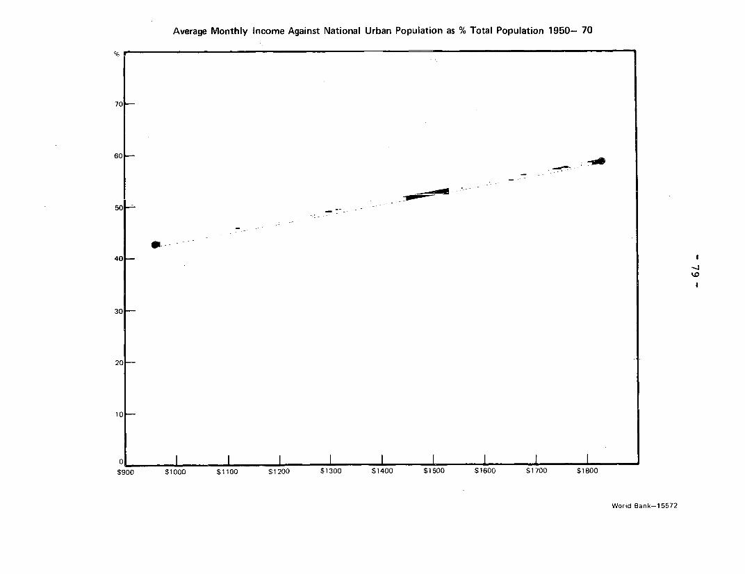
Average Monthly Income Against National Urban Population as % Total Population 1950- 70

%.

70

60 -

50

40 -

30 -

20-

10

$900 $1000 $1100 $1200 $1300 $1400 $1500 $1600 $1700 $1800

World Bank-15572

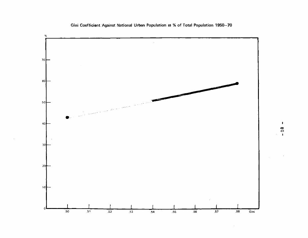
Gini Coefficient Against National Urban Population as % of Total Population 1950-70

70-

60

50

40I

3C _~~~~~~~~~~~~~~~~~~~~~~~~~~~~~~~~~~~~~C

30

20

10

O l l l l l l l I ...50 .51 .52 .53 .54 .55 .56 .57 .58 Gini

- 81 -

those which had grown more slowly. Recent rapid growthappears moreover to have had a worsening effect on thedistributive structure.

296. There was a clear relationship between contrastsin income level and differences in economic structure interms of the sectoral structure of employment. In general,the fast-growing industrial cities were better-off than others,and fast-growing cities with primarily commercial economies(such as Tijuana) also had relatively high average incomelevels. Generally, the economic dynamism of the city was thepredominant factor in accounting for income differentials,although at the sub-sector level the industrial cities whichwere associated with "modern" branches of manufacturing weremore dynamic than those with more "traditional" industrialstructures. They had consistently higher income levels thanother cities - with the exception of those on the U.S. frontier.

297. With respect to the relationship between income andunemployment, the 1970 census shows that only 3.7 percent ofthe economically active population (defined as all those aged12 and over - equivalent to 13 million people) was openly un-employed. But only 81 percent of the nominally active populationwas employed for more than 9 months of the year and a largeshare were engaged in activities at low levels of productivity,i.e., they were employed but they were only marginally productive.

298. About 45 percent of the labor force in 1970 is estimated(Trejo et al 1973) t:o be marginally employed (includes allactivities in which monthly income is less than the minimum wage).Those concerned were mainly "engaged" in agricultural or tertiaryactivities.

299. Table 14.21 shows varying levels of underemployment(defined as inactivity over a 9-month period). Cities with highlevels of underemployment were Mexicali, Oaxaca, Culiacan andVillahermosa. Some of the suburbs of Mexico City also had veryhigh levels, rising to 60 percent in one instance. Cities withlow levels of underemployment were Monterrey (16 percent),Tampico (19 percent) and some of the other suburbs of MexicoCity (as low as 15 percent).

300. There was no apparent relationship between urban sizeand underemployment. Implicitly, however, there was a closerelationship between urban growth and underemployment inseveral cities, including Hermosillo, Oaxaca, Villahermosa,Culiacan and Acapulco, but underemployment was also high inless demographically dynamic cities such as Toluca and Ciudad

- 82 -

Obregon. Rapid population growth has often been associatedwith the development of economic activities which were notlabor absorptive. A test of this hypothesis derives fromthe incidence of underemployment in the fast growing citiesin fast urbanizing states, in which services were a "leading"urban sector, such as in the states of Baja California,Sonora, Chihuahua, Tamaulipas and Nuevo Leon - all in thenorth - and to some extent also in Veracruz in the south.Table 14.21 shows the percentage level of underemploymentin each of the cities (among the 37) in these states, theidentity of the leading sector in each state and city andthe rate of urban population growth in both the states andthe cities concerned. In all of the cities of the sixstates, the level of underemployment exceeds the averagefor the largest cities as a group. The major cities inBaja California - Tijuana and Mexicali - are heavilyspecialized in tertiary activity. Both had relativelylow participation rates - Mexicali in particular. In bothcities the minimum wage was relatively high. Mexicali wasstrongly associated with the service sector, and at thesame time had the highest minimum wage of any city in thecountry and the highest level of underemployment. It wasalso one of the fastest growing cities in Mexico in 1940-70.The data in Table 14.21 suggest that a similar, though lessconsistent, association between underemployment, rapidgrowth and service sector development could be made for anumber of other cities.

(ii) Other Indicators of Welfare

301. Differences between cities with respect to incomeand income distribution imply contrasts in living conditionsalthough, theoretically, public expenditures could be usedas a countervailing instrument to offset differences inincome levels and thereby affect living standards.

302. Four types of indicators were used to examine thepattern of living conditions in the 37 cities: health andnutrition, housing, education, and non-basic goods andservices (telephones, electricity and automobile ownership).Table 12.2 presents the basic data.

303. The pattern of non-meat consumption revealed thatDurango and San Luis Potosi ranked lowest, while Mexico City,

- 83 -

Cuernavaca, Puebla, Veracruz and Villahermosa fared thebest. 1/ The infant mortality index showed a range aroundthe central value of Mexico City (1.00) and from 0.32 inCuliacan to 1.82 in Leon, a pattern for which there isno obvious explanation. Although it was generally congruentwith the pattern of meat consumption (r2 = .78) it supportsthe validity of the a priori relationship between nutritionand health.

304. Quantitative indicators of medical services showthat among the 37 cities, the large cities do not always havethe highest levels of services. Three indicators wereexamined: number of beds, number of doctors and number ofnurses in public hospitals (SSA, 2/ state and municipal andIMSS 3/) per 10,000 people. The high ranking cities (mostof the three indicators within the ten best) were: Saltillo,Torreon, Pachuca, San Luis Potosi, Hermosillo, Orizaba,Veracruz, Jalapa, Merida and Mexico City. The lowest levels(most of the three indicators within the seven worst:) werein Mexicali, Tijuana, Ciudad Juarez, Irapuato, Mazat:lan,Matamoros and Minatitlan.

305. Persisent difficulties in the housing sector inMexico have arisen from continuing pressures on supply inview of the high rate of urban immigration and the i.imitedscope of public assistance.

306. A 1962 housing survey showedthat 37 percent ofurban housing covered an area of less than 50 m 2, and thatabout 40 percent of the housing stock had only one room.It also showed that. about 6 percent of urban dwellingslccked access to water, 24 percent lacked drainage, andabout 10 percent had no electricity. In the 1970 census,a large amount of housing still lacked access to water anddrainage and about 10 percent still lacked electricity.

1/ There was an apparent relationship with meat production;most of the cities which ranked low on this index wereeither in meat-producing areas or had high income levels -

Pachuca being the only exception.

2/ Ministry of Health and Social Security.

3/ Social Security Institute.

- 84 -

307. The housing "indicators" were not, in all cases,correlated with each other. The overcrowding index showedthat the worst conditions were found in Acapulco (53 percentof all dwellings had only one room), and Villahermosa (where50 percent of all dwellings had only one room), and the bestin San Luis Potosi (18.7 percent of dwellings with one room).The three water supply indices were mutually compatible.They showed that the largest numbers of units without indoorwater supply were in Mexicali (33 percent), Matamoros (33percent), Mexico City (32 percent), and Oaxaca (35 percent).When related to population, the pattern was somewhat different.The percentage of population without access to water was 45percent in Culiacan and Minatitlan and 53 percent in Villa-hermosa, and dropped to 6.2 percent in Monterrey and 8.2percent in Mexico City. This implies that in some citieswhere access to water was poor (as in Mexico City), theaggregate level of available water was more satisfactory.In other cases (such as Tijuana) where the conveniencelevel was relatively high, the aggregate availability ofwater was poor. There was a third category of cities, ofwhich Oaxaca is an example, with approximately the same"convenience" and "aggregate" levels.

308. Except in cities with no access to water, the shareof those without piped water and without indoor water supplywas higher in Mexico City than in many smaller cities. Thesame was true of Monterrey but not of Guadalajara. Conversely,some of the smaller cities (San Luis Potosi, Durango) wererelatively better-off in spite of means used to measure condi-tions.

309. There is general, but not conclusive, evidencethat some of the fastest growing cities had the pooresthousing conditions. This was conspicuously true in theborder cities of Mexicali, Ciudad Juarez, Reynosa, NuevoLaredo and Matamoros, all of which had more than an averageshare of population without indoor water in 1970. Some ofthe most demographically dynamic cities, which were also,in most instances, economically dynamic, had some of thepoorest housing conditions. Conversely, slow growing andeconomically "backward" cities, such as Durango, had muchbetter conditions.

310. Three indicators of primary education wereexamined: (i) number of students per class, (ii) the rateof graduation in the first and sixth grades and (iii) thepercentage of the population without schooling. The citieswith the smallest number of pupils per class (a proxy ofschooling environment) were: Morelia, Mazatlan, Matamoros,

- 85 -

Orizaba and Jalapa., Those which had the highest rate ofgraduation were Torreon, Guadalajara, Cuernavaca, Villahermosa,Tampico and Mexico City. For the third indicator, Chihuahua,Pachuca, Monterrey,, Orizaba and Mexico City had high scores.Generally, the first indicator and the other two do notcoincide. The quality of primary education is reflectedin the second indicator. The medium-sized cities generallyhad high to medium scores in other urban services, with theexception of Villahermosa.

311. The cities which had poor ratings on the firstindicator (class size) were Irapuato, Monterrey, NuevoLaredo, Coatzacoalcos and Minatitlan. In the second category(the passing rate of the first and sixth grades), low ratingswere found in such cities as Durango, Toluca, and Merida.For the third indicator, the poorest group consisted ofIrapuato, Leon, Acapulco and Queretaro. While those whichhad low scores on the second indicator generally had poorratings on the other two indicators. In most of thosewhich had poor scores on the third indicator, there was afairly high level of migratory population growth during1960/70. The cities with the highest percentage of thepopulation with some secondary education included Monterrey(18 percent) and Mexico City (20 percent), while those withthe lowest were Leon (8 percent), Irapuato (7 percent),Villahermosa (9 percent) and Minatitlan (9 percent).

312. On the higher education index, Monterrey (25 per-cent) and Mexico City (33 percent) scored highest, whileLeon (8 percent) and Irapuato (6 percent) scored lowest.

313. The relationships between these indicators andurban size emphasized the relatively better-off status ofthe largest cities. There was no special relationshipbetween education levels and population growth. Nor wasthere a general relationship to economic structure, althoughthe index of professionally and technically qualifiedpersonnel per 1,000 persons appears to be related to (a)the significance of industry in the urban economy (Saltillo,Tampico), or (b) the existence of important administrative/political functions in the city (Jalapa, Guadalajara, MexicoCity), and in some cases to both (Puebla, Veracruz, Monterrey).

314. On the first index of telephone use (telephonesper 1,000 population), Acapulco (89), Mexico City (87) andCuernavaca (82) andi Monterrey (74) had the highest scores.The second and third indices which, respectively, includeand exclude Mexico City, show patterns similar to the firstas well as to each other.

- 86 -

315. This index is probably a fairly good measure ofrelative prosperity and/or economic structure. The formerexplanation seems in order for Mexico City and Monterrey.There is an a priori link with the importance of the tourismsector for Acapulco and Cuernavaca. The third index (exclud-ing Mexico City) shows a general relationship with relativeeconomic change. Thus, Hermosillo, Mazatlan and Chihuahuahave high indices while Oaxaca and Leon have low indices.In view of the national effort to improve the telephonenetwork, the increase in the number of telephones during thepast seven years has been such that cities which had a smallnumber of telephones in service had generally high rates ofincrease (Queretaro, Reynosa, Coatzacoalcos and Minatitlan).Acapulco and Tampico, however, had both a high level oftelephone service and a high rate of increase. There wereno concomitant relationships between telephone installationsand urban size or urban growth.

316. The Comision Federal de Electricidad (CFE) andthe Compania de Luz y Fuerza del Centro, S.A. (Centro) arepublic enterprises which provide electric power throughoutthe nation. 1/ CFE generates power and distributes iteverywhere, except in Mexico City and the surrounding area,which is supplied by Centro. All urban areas are coveredby the supply network. In general, fast growing cities,with the exception of the largest and of Mexico City, appearto be less well off than others. This is consistent withthe high demands of rapid population growth on the capacityof the public sector to keep up with the growing demand forpublic services. With some exceptions, particularly MexicoCity, the public sector has not allocated resources tocompensate for the consequences of rapid demographic growth.Nor has the public sector tried systematically to offsetincome differentials and the welfare consequences of contrast-ing economic structures by providing public sector servicesin urban areas which are unable to absorb an increasinglabor force.

317. The highest level of residential electricityconsumption occurred in Mexicali, Tijuana, Ciudad Juarez,Nuevo Laredo, Matamoros, Reynosa and Mexico City. Theprominence of the northern border cities is striking. Thelowest levels of consumption were in Durango, Toluca, Moreliaand Oaxaca. The cities with the highest levels of residentialconsumption were not in all cases those with the highestpercentage of homes with electricity.

318. Finally, the automobile indices show substantialdifferences. The absolute number of registered automobilesin each city showed a wide variation - from 620,800 in Mexico

1/ There is a small amount of private generating capacity too.

- 87 -

City to 1,700 in Mi.natitlan. When related to population,Mexico City (72) had a lower index than Mexicali (82), andMinatitlan (18) had a higher value than several othercities, including Ciudad Juarez and Matamoros. This pointsto interesting cont:rasts among the border cities. When thevalue for Mexico City is excluded from the calculation, thedominance of Mexicali was greatly increased (2.22) whileTijuana (1.84), Mexico City (1.95) and Pachuca (1.89) alsohad high scores. The lowest values occurred in Matamoros(.30), Nuevo Laredo (.35) and Irapuato (.46).

(iii) Income and Welfare: Conclusion

319. A factor analysis of socio-economic welfare condi-tions, based on selected indicators, is in Annex G. Thehighest overall mean score, implying the best socic-economicwelfare conditions, was that of Mexico City, followed byTorreon, Veracruz, Tampico, Guadalajara, Chihuahua andMonterrey. The lowest was that of Minatitlan followed byOaxaca, Culiacan and Villahermosa.- Key factors extractedby means of a principal component analysis indicate thattwo of the four leading factors showed particularly signi-ficant variations. These referred to (a) "conveniences"and (b)"necessities" in terms of the quality of urban life,the former category being weighted by such indices aselectricity supply and telephone services, while the latteremphasized water supply, housing and nutrition indicators.There were strong inter-city contrasts with respect: to both.The border cities scored high in terms of convenierLces butpoorly in terms of;necessities. Other northern cit:ies were,in general, well-off with respect to both factors. Thecities of the central zone (the belt stretching fromGuadalajara to Veracruz and including Mexico City) showedstrong contrasts. Most cities in the western portion ofthis zone, with the exception of Guadalajara, were relativelybadly off compared with Mexico City and other surroundingurban areas. Cities to the east of Mexico City, with thenotable exceptions of Minatitlan and Villahermosa, alsofared comparatively well. By contrast, cities to the southof this central zone were, without exception, less well offthan those of either the north or the center with regard toboth conveniences and necessities.

320. Though relationships between these contrasts in socio-economic welfare and the economic and demographic characteristicsof the largest cities do not show consistent patterns, it isworth mentioning that the welfare index is positively correlatedwith city population and income level.

- 88 -

4. THE SPATIAL STRUCTURE OF TIIE URBAN SYSTEM

321. The spatial implications of the urban system maybe analyzed in terms of the area of economic development andin terms of the regional aspect.

322. The area aspect concerns variations in developmentacross the spatial surface of the national economy. It hascertain constraints because it can only be measured in termsof statistical areas for which consistent time series dataare available (includes the 32 states of the Federation).

323. The regional aspect is also based statisticallyon these units because the only means of developing a setof regions is to aggregate states. 1/ The key to regionaldemarcation is provided by the spatial structure of theurban system. The fundamental precept is that the spatialorganization of a systemic economic structure is determinedby the relationships between its principal cities, which arethe major locations of production and consumption, and themost important central places in the national economy. Forthe purpose of regionalizing the country, the set of 37 citiesis larger than need be, because the spatial structure can beadequately defined in terms of a smaller set of urban places.

324. The objective of this chapter is twofold: (1) torelate the patterns of area development from 1940 to 1970to the level of urbanization in each state and to the spatialdistribution of large cities between states; and (2) toconstruct a set of economic regions defined in terms of stateaggregations and built around the spatial framework of thenation's urban system.

A. Area Development and the Structure of the Urban System

Demographic Structure

325. The interstate distribution of the urban populationin 1940-70 is shown in Table 1.15. Certain states maintainedalmost exactly the same shares of the nation's urban popula-tion throughout the period. Thus, while the urban populationof the Federal District increased from 1.6 million in 1940to 6.6 million in 1970, and accounted for 23.9 percent of thenation's urban population in the former year, it accountedfor 23.5 percent in the latter. Jalisco also retained aroughly constant share of the urban population (8 percent),as did Veracruz. But there were important changes in Baja

1/ It would, in theory, be possible to do so on the basis ofmunicipalities but this would be extremely time consuming.

_ 89 -

California (0.6 percent to 2.6 percent), Coahuila (4.0 per-cent to 2.9 percent), Nuevo Leon (3.4 percent to 4.6 percent),Puebla (5.2 percent to 4.1 percent) and Yucatan (3.0 percentto 1.7 percent). Most of the states with very smaLl sharesof the urban population at the beginning of the period(Colima, Nayarit, Queretaro, Quintana Roo) also hadi verysmall shares at the end.

326. The absolute size of the urban population in eachstate in each census year and the average intercensal compoundgrowth rates are shown in Table 1.16. These data explainshifts in the distributive structure. Baja California, forexample, had the i-astest rate of urban growth of any statein the nation during 1940-70, but this growth began from arelatively low base in 1940 implying that its share of urbanpopulation was still fairly small in 1970. The relativerate of urbanization in each state and the rank order ofthe rate of urbanization in each intercensal period areshown in Table 1.17.

327. The states with the largest shares of the urbanpopulation in each year were not necessarily the most urban-ized. By 1970 the most urbanized states (classified asthose more than 7( percent urbanized) accounted for a muchlarger share of the total urban population than in earlieryears (Table 1.19).

328. The rate of urbanization at the state level wasnot closely assoc:iated with the share of the urban populationat the beginning of each intercensal period, an implicationconfirmed by correlation analysis (Tables 13.16 and 13.30).Some of the least urbanized states in 1940 were among thosewhich urbanized most rapidly during 1940-70, notably BajaCalifornia. Conversely, some of the most urbanized states(in terms of the share of the total urban population andof the level of state urbanization) were among those whichurbanized rather :,lowly after 1940. In the Federal District,for example, the absorptive capacity of the state had beenreached before 1970. Obviously, as the "level" of urbaniza-tion approaches 100 percent, the rate of urbanization mustfirst slow down and eventually halt.

329. Changes in the relative distribution of the urbanpopulation and geographic contrasts in relative rates ofurbanization necessarily reflect differential patterns ofnatural increase and migration (Annex H). Table 1.56demonstrates that 1970's largest cities accounted for avery large proportion of urban demographic development.There were, howevzer, significant interstate contrastsderived from: (a) different rates of urbanization, and(b) intrastate urban structures.

- 90 -

330. There were several instances of slowly urbanizingstates in which cities among the nation's 37 largest in 1970,did not account for a large share of the total urban population.These included Guanajuato, Hidalgo, Michoacan and Oaxaca. Inaddition, there were eight states or Federal Territories whichdid not include one of the 37 cities. These were: Baja Cali-fornia Sur, Campeche, Colima, Chiapas, Nayarit, Q. Roo,Tlaxcala and Zacatecas. Generally, there were few largecities in the slowly urbanizing states and even where largecities did occur, they did not account for an important shareof the total urban population.

331. Conversely, the fastest urbanizing states had oneor more of the nation's largest cities, which accounted fora large share of the urban population of the state concerned.There were some states (such as Yucatan and Puebla) in whichthe largest city or cities accounted for a large share of theurban population, notwithstanding that the state did not,during this period, undergo rapid urbanization. A largeshare of the state's urban population could thus be accountedfor, either by rapid urban-size-growth or by the presenceof a large city, irrespective of the latter's rate of growth.

332. The nation's largest cities generally accounted forall or most of the urbanization in their respective states.In the Federal District 100 percent of the urban populationwas located in the metropolitan area of Mexico City. Else-where, 75 percent or more of state urbanization was accountedfor by the urban hierarchy in Baja California Norte, Jalisco,Mexico State, Nuevo Leon, Tamaulipas, and Queretaro. Allwere rapidly urbanizing states in 1940-70, and all werehighly urbanized by the end of the period.

333. In sum, the geographic distribution of the majorcities of the urban hierarchy "accounted for" major contrastsin the geographic distribution of the urban population by1970, and spatial contrasts in urbanization were largely"accounted for" by the differential growth of the nation'slargest cities.

Patterns of Area Development

(a) Area Development and Urbanization

3a4. Against the background of detailed data presentedin Annex I, a composite developed index relates the spatialvariations in urbanization.

- 91 -

335. The variables of the index are: (1) state product -per capita; (2) industrial output as a share of state product;(3) industrial employment as a share of total employment; (4)capital investment in agriculture; (5) irrigated areas as ashare of the cultivated area; (6) electricity consumption percapita; (7) gasoline consumption per capita; (8) infantmortality per 1,000 live births; (9) sugar consumption percapita; (10) percentage of houses with water; (11) percentageof population with shoes; and (12) literacy.

336. Table 3.14 shows that state development resflectedtrends in the national economy and that progress was farfrom even. Twenty-four states maintained the same rank over30 years. But Baja California Sur, Mexico, Tabasco, Sinaloaand Morelos all improved on their initial ranks while Yucatan,Quintana Roo and Durango lost in relative status. Thesechanges, however, dlo not fundamentally alter the generalpattern of relative stability.

337. The Federal District retained the first rank atall times. The same states were ranked 1-9 throughout theperiod, with the exception of Aguascalientes (in 1950) andBaja California Sur (in 1970). Similarly, Oaxaca remainedat the bottom from 1940 through 1970 and the same states(Oaxaca, Chiapas and Guerrero) occupied the last threeranks each year.

338. In geographic terms, these data show that eightof the fourteen most developed states were in the north,and that three of the others were around Mexico City(Distrito Federal, Mexico, Morelos) and one was in thePacific Southwest (Jalisco). In contrast, almost all ofthe poorest states were in the south. Most of the statesin the "intermediate" category were geographically betweenthese extremes. This suggests a three-tier pattern ofdevelopment broken only by the fact that part of thecentral area (around Mexico City) and Jalisco, fell intothe highly developed rather than the intermediate category.

339. Thus spatial contrasts in urbanization wereconsistently associated with spatial development. Withrespect to 1940 (Table 13.11), the relative index ofstate development is highly correlated with the levelof urbanization (r2 = .75). In 1970 (Table 13.12), theassociation was even stronger (r2 = .85). This findingis confirmed by the fact that relative developmentmeasured on the basis of income level was also stronglyrelated to urbanization (Table 13.13).

- 92 -

340. The fact that the degree of association betweenrelative development and relative urbanization was close inboth 1940 and 1970 but closer in the latter year than theformer, suggests that a time trend analysis would reveal aclose relationship between the trend of state developmentand the trend of state urbanization.

341. This hypothesis was tested by using the same twelvecomponent index as a dynamic measure of relative developmentshowing trends in the relationships between the developmentlevels of each state over three decades (Table 3.15).

342. These measurements are based on the position ofeach state relative to the Federal District, the highestranking state in each year, and the tendency towards increas-ing disequilibrium vis-a-vis the Federal District, in thestates of the South, moderate disequiibrium in those of theNorth and a variable situation in the states of the center.(See Map 28).

343. Table 3.5 shows that the states which, in 1940,were relatively most developed, tended to maintain theirstatus relative to other states. The trend for the wholeperiod indicates that the states which suffered the leastamount of change relative to the Federal District were thehighest ranking in terms of differential development vis-a-visthe Federal District in 1970, although Baja California Nortestands out as an area which developed more rapidly than anyother. Conversely, the lowest ranking states in 1970 werethose in which the annual rate of differentiation vis-a-visthe Federal District was greatest - notably Quintana Roo andZacatecas. However, some of the states which had intermediatelevels of development also experienced rapid deteriorationin relative status, the outstanding instances being Durangoand Yucatan.

344. Thus differentiation increased over time and thatdifferentiation was, in general, accentuated in those stateswhich were, at the beginning of the period (1940), among thepoorest.

345. A comparison of state trends in urbanization withstate trends in development confirmed that there was a dynamicrelationship between relative development and relative urbani-zation. Tests showed that the states (led by Baja CaliforniaNorte) which urbanized most quickly after 1940 were thosewhich developed most quickly. This corresponds to the patternwhich has been characterized by Myrdal (1957) as one of"circular and cumulative causation".

- 93 -

346. Because urbanization and area developmentl wasgenerally related, and urbanization and the urban hierarchywere generally related, a general association is presumedto exist between area development and the urban hierarchy.

347. The validity of this assumption is obvious in thecase of the Federal District and in such states as BajaCalifornia Norte and Nuevo Leon where large and prosperouscities were located in (and accounted for the prosperity of)relatively prosperous states.

348. There were, however, some instances of disjunctionbetween area development and the development of major cities.First, there were some states where the level of areadevelopment was higher than expected, assuming a generalcorrelation between urbanization, the urban hierarchy, andarea development; in all such cases, however, there wasrapid urbanization in 1940-70. Second, there were somestates in which the level of urbanization was low andcompatible with the level of relative area development -but in which there was one or more large city. Ge:nerally,large cities develop associations with smaller cities intheir hinterlands and with rural areas. Consequently, thestate as a whole undergoes economic development. In somestates, however, large cities were associated with relativelylow levels of area development, which relates to thestructure and the development of the rural sector.

(b) Urban Development Without Area Development

349. Certain conditions govern the spatial diffusionor "spread" of the benevolent effects of urbanization. Forexample, a city whose locational rationale is the existenceof a mineral resource but which is located in the middle ofan arid and unirrigated plain may, for as long as theresource base endures and is in demand, continue to grow.Its development wiLll not however "cause" the developmentof the hinterland. Generally if the physical, economic andsocial conditions of an area surrounding a city do notfacilitate the diffusion of development, such diffusionwill not take place. In Mexico, the areaswhich lackfavorable conditions for agricultural development generallyare not penetrated by the diffusion of development impulsesfrom the urban sector. In several states, the presence ofa large city does not coincide with a high level of overalldevelopment at thes state level, and there is a disjunctionbetween relative urban development in terms of urban sizegrowth, and relative area development. The spatial structureof the agricultural sector seems to be the key to explainingsuch disjunctions.

- 94 -

350. Table 13.15 suggests that, in general, the lessurbanized states also had low levels of agricultural develop-ment. Disjunction between urbanization and area developmentwith a correlate in agricultural development is more apparentwhen urban development is considered in terms of the existenceof large cities located in relatively unurbanized and under-developed states. Three cases are outstanding: the statesof Mexico, Puebla and Guanajuato. In each of these statesthere is a large city. In the state of Mexico, there ispart of Mexico City; in Puebla, there is the city of Pueblaand in Guanajuato, there is the city of Leon. The overalllevel of urbanization in each of these states in 1970 wasrelatively low: 23 percent in Mexico, 28 percent in Pueblaand 35 percent in Guanajuato. The overall development indexwas also relatively low: -3.1 in Mexico, -3.3 in Puebla,and -2.5 in Guanajuato. In each, the indicators of agri-cultural development were low. In terms of capital investmentper agricultural worker for example Mexico, Puebla andGuanajuato ranked 23rd, 25th and 24th out of 32 states.In terms of labor productivity, they ranked, respectively,19th, 30th and 32nd. In spite of the presence of large,industrialized urban areas in each state (which ranked, inthe order given above, 2nd, 6th and 7th, with respect torural population density), it seems likely that the condi-tions of the rural sector impeded the diffusion of thebenefits of urban industrial growth. It also seems thatthe conditions of the rural sector may have impeded thediffusion of urbanization per se, inasmuch as in thesestates a very large share of the total urban populationwas concentrated in the largest city.

(c) Area Development Without Urban Development

351. Spatial contrasts in the structure of agriculturalproduction and income have influenced population movementsand particularly outmigration. There has been a closerelationship between outmigration and a series of indicatorsof rural/agricultural conditions. Heavy outmigration fromChiapas, Oaxaca and Guerrero was associated with a lowrelative level of agricultural development (Table 8.6).

352. At the same time, net migration in other stateshas been positively correlated with a high level of agri-cultural development. This applied particularly to thenorthwest (Sonora, Sinaloa, Baja California), and suggeststhat migratory movements were associated with high levelsof agricultural development. In these states, the growthof output was not linked with land reform or with thedevelopment of the "traditional" sector but with large-scaleirrigated commercial agriculture, which was most thoroughly

- 95 -

developed after 1940. Although no relationship between thespatial incidence of net population change and land reform(Table 8.7) has been established, it can be argued that landreform efforts were concentrated in states with the mostsevere problems of population pressure. Although landreforms failed to resolve these problems, this is nct tocriticize the effort that was made. Otherwise, outmnigration(as an index of rural conditions) would almost certainlyhave been greater.

353. The states with the least favorable structuralconditions in agriculture generated a large proportion ofthe migrants who went to states with better agriculturalconditions or who contributed to a large share of urbanpopulation increase, thereby closely associating urbanizationwith the deficiencies of the agrarian structure of t:he statesof the center and the south (although migrants from theseareas often moved to cities far removed from their placesof origin - particularly to those in the north).

354. In-migration to the agriculturally developedstates of the north was positively associated with urbaniza-tion in another way. Table 8.8 shows that the states withhighly developed agriculture (Baja California, Sinaloa,Sonora) also ranked highly in terms of intercensal urbaniza-tion. These states had high relative levels of generaldevelopment, although they were relatively unurbanized (asmeasured by the urbanized percentage of the state population).They were major centers of in-migration and rapid urbanization,as measured by the growth of the urban population and areasof advanced agricultural development. The inter-relationshipsof these indicators is based on the timing of agriculturaldevelopment, which seems to have preceded urban development.Therefore, urban development in the northwest was,partly, aconsequence of the prior growth of irrigated commercialagriculture implying that urbanization in this region wasconceptually associated with the development of an agriculturaLexport base. This type of urban growth was a common phenomenonduring the Porfiriato, 1/ but does not seem to have occurredin other parts of the country after 1940.

1/ See Chapter 1.

- 96 -

355. The development of new industries from an exportbase depends on the nature of the base. If development leadsto the construction of large-scale infrastructure (particularlyin transport), production and distribution costs for manyactivities may be lowered. Growing internal and externaleconomies of scale will then tend to stimulate export growth,thereby expanding the base. If the external demand for aregion's product falters, stagnation will likely ensue. Itis less likely to occur if the local economy is greatlydiversified.

356. Development of the export base depends on thesuccessful generation of new activities from the original-export oriented activity. This is precisely what happenedin the northwest after 1940. Driven by massive publicinvestment in irrigation, the regional economy generatedlarge surpluses of agricultural output for the rest of thecountry and for national exports. The growth of agriculturealso generated new demands for services and, to an increasingdegree, was linked with the growth of manufacturing (withspecial reference to food processing industries). In sum,urbanization and agricultural development in this regionwere intimately linked.

B. Regional Development and the Structureof the Urban System

Regional Definitions

357. A second, and entirely different spatial dimensionof the national economy concerns its regional structure whichis defined in terms of the functional spatial framework ofeconomic interaction and exchange. We are concerned neitherwith identifying homogeneous socio-economic conditions acrossgeographic areas, nor with programatic development regions.The focus is on how the space-economy works and the organiza-tional roles of the country's major cities in that process.

358. A fundamental premise underlying this analysis ofthe urban system after 1940 has been that the system wasfully articulated, in the sense that the national economydeveloped along interdependent lines and that the nationaltransport system became sufficiently complete to facilitatemacro-geographic interaction. Thus, every part of thenation's territorial space must be related to each otherpart on the basis of access to one or other of the country'smajor cities which constitute the framework for nationalspatial integration.

- 97 -

359. There are many levels of interaction and manylevels of integration. We are concerned with macro-geographicspace (i.e., that of the nation as a whole), so the relevantlevel refers to a high order of functional interaction basedon the city as a major center of economic activity dominatingthe economy of the surrounding area. This relationship isclearly observed in the structure of the tertiary sector inmajor cities (generally, as we have seen in Chapter 2, inproportion to their size), which provide services not onlyfor their own populations and those of immediately proximateareas but also for populations at greater distances. Becauseof the link between urban size and the level of manufacturingactivity, which is generally strongest with respect toconsumer goods industries, major cities also serve as manu-facturing and distribution centers for their associated regions.

360. Assuming (a) that all parts of the nation wereintegrated in the national space economy by 1970 and (b)that integration was achieved through linkages to majorcities, there are three complementary ways of examiningMexico's spatial structure. The first focusses only onMexico City and regards the whole country as a single region.Indeed, for certain purposes it is, because of Mexico City'seconomic and social. dominance. Earlier chapters have dis-cussed the capital city's demographic, industrial, commercial,cultural and political domination. Tucker (1957) states: "InMexico, all roads lead to the capital of the country; theFederal District is the chief political and governmentalcenter of the nation. Moreover, it is the economic, educa-tional, social and cultural center of Mexico . . . itsinfluence is all pervasive. Other cities are satellitesof greater or lesser magnitude held in their orbits by thecentral sun." This aptly describes the core-peripherystructure discussed in the Preface. Table 4.17 shows thatMexico City's primate role is the single most importantfeature of the Mexican space economy. (See"Spatial Develop-ment in Mexico" for a discussion of the implications of therole of Mexico City).

361. Mexico's space economy may be seen on other levels.Map 29 shows the whole of the nation's space allocated to oneof the three largest metropolitan areas - Mexico City,Guadalajara or Monterrey. This is a realistic pattern because,while there are certain functions (those of the Federal Govern-ment in particular) which are performed exclusively in MexicoCity, other relatively high order functions are also per-formed in the second and third largest cities and not else-where. The most striking feature of this pattern is that thelargest territorial area is assigned to Monterrey. Althoughthe pattern of population density emphasizes the relative

- 98 -

dominance of the zones associated with Guadalajara and MexicoCity, particularly the latter, territory alone does not deter-mine the relative size of each zone. What it does imply isthat the zone associated with Monterrey is so vast that thepossibility of functional interaction with its western partsmust be questioned. The contiguity of the northern zonewith the US frontier is an impediment to spatial economicinteraction, but not an absolute barrier. The economies ofthe northwestern states (which are associated in this schemewith Monterrey) have developed close functional ties with theU.S.A. (See Chapter 2); consequently, a substantial part ofthe northern zone "looks" towards cities in the US borderstates including Los Angeles/Long Beach (1970 population7.0 million), San Diego (1970 population 1.4 million),Phoenix (1970 population 1.0 million) and El Paso (1970population 800 thousand).

362. These massive "zones" are not "regions" becausethey are too large to correspond to anything other thanan approximate territorial division among the three largestcities with respect to service functions.

363. The third level of spatial organization, shown inMap 30, represents an approximate urban-regional structurebuilt around major cities. The regions thus defined varygreatly in territorial and demographic size and in socio-economic conditions. They vary, too, with respect to thesize and characteristics of their central cities - orregional centers. Six major regions have been delineatedwithin the commonly accepted bounds of accuracy for regionaldemarcation. For measurement purposes, regional boundarieshave been adjusted to coincide with state boundaries. Thesix regions (some of which are subdivided to make a totalof 12 subregions) correspond to zones of general socio-economic integration representing "general purpose" regions.These do not necessarily correspond to development regions,if the latter are defined in terms of areas which can beused for integrated development planning.

364. The major regional capitals associated with theseregions are: Mexico City, Guadalajara, Monterrey, Tijuana/Mexicali, Chihuahua, Culiacan, San Luis Potosi, Queretaro,Puebla, Veracruz, Oaxaca and Merida. As with any suchscheme of allocation, there are certain anomalies.

365. The first category of anomalies consists of problemswhich arise with respect to the regional allocation of stateswhich do not include major cities, and which do not havestrongly developed linkages with any of the leading metropolitan

- 99 -

areas. These are usually either poor, or small or both,examples being Oaxaca, Chiapas, Hidalgo, Guerrero, Colima,Nayarit and Michoacan. The allocation of these states totheir respective regions is a somewhat arbitrary matter.The second problem is that some cities, the main examplesbeing Leon, Torreon and Tampico, are located on state boundaries,and their location is also somewhat arbitrary because, in aregional scheme unconstrained by,the form in which data areavailable (i.e., did not have to respect state boundaries),both of these cities would be important regional centers.These problems show that no scheme of regional allocationcan be perfect when the availability of regional informationis an important criterion (i.e., when it is necessary to beable to describe and compare the demographic and socio-economic characteristics of different regions). Yet, theurban-regional-structure on Map 30 is- generally consistentwith the basic definitional framework of the urban systemand thus represents a reasonably accurate outline of Mexico'sspatial economic structure in 1970.

366. Earlier chapters referred to more detailed aspectsof this picture. TIhe next section will expand the (descriptionof some of the key features of the regional structure interms of inter-regional contrasts and intra-regionaL charac-teristics. Table 3.17, which gives demographic, social andeconomic indicators; pertaining to each region (measured onthe basis of states), provides a key reference throughoutthis section.

Regional Profiles

(a) The Northwest

367. The four states in this region, Baja CaliforniaNorte, Baja California Sur, Sinaloa and Sonora, fall intotwo sub-groups, comprising Baja California Norte and Sur andSinaloa/Sonora, the former centered on Tijuana/Mexicali,which in this context may be thought of as twin regionalcapitals, and the latter, on Culiacan. The northwest asa whole is distinguished by its advanced level of agricul-tural development, and relatively high level of socio-economic development, but is neither highly urbanized norindustrialized. Its major cities - Tijuana, Mexicali andCuliacan - have gernerally poor social conditions with highlevels of underemployment, skewed patterns of incomedistribution and inadequate levels of service provision.

- 100 -

368. The northwest as a whole covers about 20 percentof Mexico's land area but contains less than seven percentof its population. Just as the northwest was the country'smost rapidly urbanizing area in 1960/70 (all four stateshaving achieved well above the national average rate ofpopulation increase), so too, their total populations weregrowing much faster than that of the nation as a whole.

369. Demographically dynamic, the northwest has becomean aggressive and upwardly mobile region in terms of economicperformance, with the highest levels of agricultural productiv-ity in the nation, an average per capita income level almost50 percent above the national average, and a relatively goodpattern of income distribution as measured by the Ginicoefficient.

370. Whilst these conditions apply to the region as awhole, there are sufficient contrasts between the Tijuana/Mexicali region comprising Baja California (North and South),on the one hand, and the Culiacan region comprising Sonoraand Sinaloa, on the other, to provide major sub-regionalidentities within the northwest.

371. The Tijuana/Mexicali sub-region stands out as anarea of rapid demographic expansion in the 50s and 60s,particularly in its urban areas and in terms of its economicdynamism and high average incomes per capita, notwithstandingthe relative skewness of the distributive patterns of itscore cities. A large proportion of the region's populationis concentrated in Tijuana and Mexicali (67 percent in 1970)and the twin regional capitals account for an even largerproportion of its urban population (85 percent in 1970). Theregion as a whole is strongly focussed on its core area, (seeTable 10.17, which shows that the largest proportion of roadtransport movements of the six major regional areas in 1970originated and terminated within this region). Althoughthese data also refer to the Culiacan sub-region, they arestrongly influenced by the inward-looking nature of the BajaCalifornia economy vis-a-vis the rest of Mexico. Because ofits location and economic structure, the Tijuana/Mexicaliregion has very strong linkages with the economy of SouthernCalifornia in the U.S.A. Taking account of this orientation,the sub-region is less autarkic than it seems. Distance is,and will remain, a major impediment to fuller integrationwith the Mexican economy; it still takes 44 hours to travelby road from Mexico City to Tijuana and 41 hours to travelto Mexicali.

- 101 -

372. In sum, the Tijuana/Mexicali sub-region is in manyways detached from the rest of the country. Its thrivingeconomy is a result of the development, since 1940, ofintense relations with the even more thriving and highlyprosperous economy of Southern California, but it also hasmany problems which are related to the proximity of theUnited States. The rapid growth rates of Mexicali andTijuana (See Chaptier 2) have been strongly affected bymigration from other parts of Mexico, and there is no doubtthat the principal motivation for migrating to Baja Californiahas been the opportunity to move from there to the U.S.A.While these cities are relatively prosperous, they have notbeen able to absorb the large migratory influx (see Chapter3 for a discussion of the low-level of welfare conditions).

373. The Culiacan sub-region is far more closelyintegrated with the Mexican economy than that of Baja Califor-nia. The development of prosperous agricultural economiesand of thriving cities has been closely related to the impetusof the agricultural sector in Sonora and Sinaloa, and themarket opportunities, enterprise and technological diffusionfrom the U.S.A.

374. This sub-region has also been demographically andeconomically mobile, and its core city of Culiacan has grownat a rate well above the national average. Its secondarycities - Ciudad Obregon, Hermosillo and Mazatlan - have withthe exception of t:he last, also been extremely dynamic (Table1.29). Income per capita is much higher than in the nationas a whole, and income distribution is among the most equit-able in the country, the Gini coefficient in 1970 being 0.50compared with the national average of 0.58.

375. Accessibility between the Culiacan region and therest of the country is better than that of the Tijuana/Mexicali sub-region (See Table 10.33) because of the muchshorter distance (exemplified by a driving time of 18hours from Culiacan to Mexico City vis-a-vis more than 40to Baja California), and the relatively well developedtransport services to the rest of the country.

376. Table 10.7 shows that Culiacan has relativelymore intensive linkages with the northwest (Monterrey,Monclova) and the Southwest (Guadalajara, Salamanca) thanwith Mexico City, although its intra-regional link;s (withHermosillo, Mazatlan, Nogales and Ciudad Obregon) wererelatively stronger.

- 102 -

377. The pattern of traffic to and from Hermosillo showsthat Culiacan does not dominate this sub-region to the sameextent that Tijuana/Mexicali dominatesBaja California.Hermosillo has strong links with the center (Mexico City andPuebla in particular), the northwest and the southwest. Thepattern of telephone traffic (Table 10.27) confirms stronglinkages with Mexico City, although these are notably weakerthan those of most other large cities. There are some prob-lems of data interpretation because railroad freight movementsinevitably emphasize the long journeys and de-emphasize intra-regional movements; the same shortcoming applies to thepattern of air-traffic (Table 10.26). The data do suggestthat the Culiacan sub-region is less closely tied to MexicoCity than most other regions, but that it is more closelytied to the rest of the country than the Tijuana/Mexicalisub-region.

378. The northwest, a large, loosely integrated,prosperous and generally dynamic area which is not stronglydominated by its largest city, is generally well connectedwith the rest of the country. Its ties with areas otherthan the center, however, are weaker than those of mostother parts of the periphery.

(b) The North

379. Again there are two sub-regions, one including thestates of Chihuahua and Durango with a regional center inChihuahua City, and the other including the states ofZacatecas, Aguascalientes and San Luis Potosi, with aregional center in the city of San Luis. The region, asa whole, has little homogeneity and is most validly dis-cussed in terms of its two sub-regions.

380. The first sub-region is extensive, occupying almost20 percent of the national territory with less than 5.0 per-cent of its population. Sparsely populated, it is not adynamic region. Its rate of population growth in the 1960swas lower than that of other parts of the northern zone, aswas its rate of income growth. It is relatively well-offcompared with most other parts of the country. Consistentwith the general finding that income levels and incomedistribution are inversely related, its Gini coefficientis relatively high.

381. Compared with the center and the south, theChihuahua region is not heavily urbanized and its urbanstructure is strongly dominated by Chihuahua and CiudadJuarez. The latter is considerably larger than Chihuahua

- 103 -

but is not a regional capital because of its frontier location.Its economy, as in Tijuana and Mexicali, is closely linkedwith the United States. Road traffic data indicate that theregion as a whole (i.e., including the San Luis sub-regionas well as the Chihuahua sub-region) appears to be stronglyintegrated with the northeast (Table 10.17) but has relativelyweak connections with the northwest, the west and the center,and hardly any at all with the south. Rail traffic data inTable 10.7 show linkages between Chihuahua and other partsof the country, while Ciudad Juarez appears to have stronglinkages with both the center (Mexico City, D.F.) andGuadalajara. These, however, are related to through trafficfrom the U.S. rather than to traffic originating in the CiudadJuarez area. The structure of the strictly inter-regionalflows is less distorted than would appear.

382. Linkages with the center are an important partof the total air-traffic pattern. As in the northwest,traffic with Mexico City accounts for the smallest shareof regional traffic (Table 10.26).

383. The second sub-region of the northern zone is, bycomparison with the first, much smaller (occupying 'Littlemore than seven percent of the country's land area), moredensely populated (particularly in Aguascalientes), lessurbanized, and poorer. Agricultural productivity, exceptin Aguascalientes, is very low. Agriculture provides morethan half of all employment in this region, so the levelof per capita income is well under the average for northernMexico as a whole, and is only slightly above that of thesouthern states. Consistent with our earlier findings,income is poorly distributed, the average Gini coefficientbeing above 0.60.

384. This sub-region is quite strongly dominated bySan Luis which is its largest city, the only other sizableurban center being Aguascalientes.

385. Intra-regional rail traffic between San Luis andother cities shows quite strong linkages with Aguascalientesand Zacatecas, although it also shows that the region has astrong relationship with the ports of Tampico and Matamorosand with the inland cities of Monterrey and Nuevo Laredo,all of which are inithe northeast. This suggests that not-withstanding the relative geographic proximity of the SanLuis region to Mexico City and to the states of the center(San Luis is only five hours by road from the capital), itshould be regarded as part of northern Mexico, as it isclassified here.

- 104 -

(c) The Northeast

386. Occupying nearly 15 percent of the nation's terri-tory this region is one of the best integrated in the country.It contains several major cities besides the regional capitalof Monterrey, including Nuevo Laredo, Reynosa and Matamoroson the U.S. frontier, the port of Tampico in the southeastcorner of the region, and Saltillo and Torreon in the west.Its population amounts to more than eight percent of thenational population, but because this is a highly urbanizedregion, its share of the nation's urban population exceeds11.0 percent. It is, concomitantly, prosperous. More than25 percent of its population is employed in manufacturing,as compared with an average of 14 percent in the northernstates as a whole. Its prosperity is also linked to unusuallyhigh agricultural productivity. Per capita income is con-sequently well above the national average, although the Ginicoefficient is comparable to that of the northern states asa whole. This region is both demographically and economicallydynamic, having had higher rates of population growth andincome growth than most other regions during the 1960s.

387. Rail freight data (Table 10.7) suggest that thenortheast is integrated strongly internally and that it alsoenjoys powerful linkages with all other parts of the country,particularly the central region. This is borne out by airpassenger traffic (Table 10.24) and road freight traffic(Table 10.17), although the latter suggests strong connectionswith the northern region. The pattern of telephone traffic(Table 10.27) underlines the importance of both intra-regionallinkages and connections with the center.

388. This is, in sum, a large, prosperous, upwardlymobile and well integrated region enjoying a large internalmarket, close connections with the U.S.A. (which providesits northern frontier) and strong linkages with the rest ofthe country, emanating from its unchallenged regional capitalin Monterrey.

(d) The West

389. A comparison between the west and the northeast isof interest because these regions are dominated by thecountry's second and third largest cities which differ socio-economically and structurally.

390. Territorially, the western region is not very large.But it contains about 10 percent of the nation's populationand, in the 1960s, was one of the most demographically dynamic

- 105 -

growth areas in the country. However, despite the presenceof almost one and half million people in Guadalajara in 1970,the southwest was less urbanized than might be expected. Itsurban population was about the same as the national average,while its rate of urbanization in the 1960s was somewhatslower than that oi- the nation as a whole. Employment inagriculture was about the same as the national rate butagricultural productivity was relatively higher, and itsshare of manufacturing employment in 1970 was less thanproportionate to its share of total employment, suggestingthat agriculture was the mainstay of the region's economy.Notwithstanding reLatively good productivity, average incomesper capita were beLow those of the northern and central states,while the distribution pattern was relatively favorable.

391. Whereas the northeast, excluding Monterrey, boastsa number of large metropolitan areas which provide a strongframework for regional integration and growth, the west doesnot. At a regional level, Guadalajara is a strongly primatecity, being more than 10 times as large as Morelia, the onlyother city of more than 100,000 people in this region.

392. Rail traffic movements suggest strong patterns ofinter-regional interaction with the northwest, particularlywith the Culiacan sub-region, the Federal Capital regioncentered on Mexico City, and the Bajio region which (seebelow) lies between Guadalajara and Mexico City with whichit enjoys a high level of relative accessibility (Table 10.30).The pattern of road freight traffic (Table 10.16) alsoemphasizes the importance of linkages with the Chihuahuasub-region to the north, by the air passenger trafific matrix(Table 10.24) and by the telephone traffic matrix (Table10.27).

(e) The Center

393. Although Mexico City is the functionally dominantcenter for the whole of the central region - an area whichincludes the States of Mexico, Morelos, Guanajuato, Queretaro,Hidalgo, Puebla and Tlaxcala, as well as the D.F. - thereis sufficient diversity within this region and a sufficientnumber of functionally effective regional centers, to lead usto identify three sub-regions. The first includes the D.F.,Mexico and Morelos, with its center in Mexico City; thesecond, Guanajuato, Queretaro and Hidalgo with its centerin Queretaro and t:he third, Puebla and Tlaxcala, with itscenter in Puebla.

- 106 -

394. Before examining the characteristics of each ofthese sub-regions, we shall briefly consider the diversityof the region as a whole and the nature of its relationshipswith the rest of the country, especially as articulatedthrough Mexico City.

395. The central region covers less than eight percentof the Republic's area but contains no less than 36 percentof its total population, almost 25 percent of which is inthe D.F. and the State of Mexico. The presence of MexicoCity and of many other large metropolitan areas, includingQueretaro, Leon, Irapuato, Pachuca, Toluca, Puebla andCuernavaca, result in a highly urbanized region, with morethan 70 percent of its population urbanized in 1970. Thusit is a densely populated region, with by far the highestdensity of any part of Mexico. Yet it is also diversebecause, outside Mexico City, the states of Queretaro andGuanajuato and Puebla remain largely rural, while thepopulation density of Queretaro and Hidalgo is notablylower than that of the region as a whole.

396. In the recent past, it has been a less dynamicregion demographically speaking than most of northernMexico, with the notable exception of the States ofQueretaro, Mexico and Morelos.

397. Despite the largely urban nature of the centralregion, agriculture remains the source of livelihood formuch of its population, accounting for half or more of totalemployment in Hidalgo, Guanajuato, Puebla and Tlaxcala.Agricultural productivity, particularly in Morelos, isgenerally high. The average income is above 150 pesos/hain all parts of the region except Tlaxcala. The manufactur-ing and tertiary activities of the central region are itsdistinguishing feature, accounting for more than 50 percentof all manufacturing employment in the nation and an evenlarger share of tertiary employment in 1970.

398. One would therefore expect that income per capitawould also stand out in a comparative context as in theFederal District (Chapter 3). But, this is not the case inmany other parts of the region; Guanajuato, Hidalgo, Puebla,Queretaro, Morelos and Tlaxcala all have relatively lowincome levels with relatively skewed patterns of incomedistribution. It is this, rather than the relativelyfavorable aggregative indices of its employment structure,which reveals the intense contrasts in socio-economicwelfare in the central region. For the most part, thesevariations arise from the highly unequal pattern of landdistribution in the rural sector and the widespread rural

- 107 -

poverty which occurs within the framework of high avreragelevels of agricultural productivity.

399. As expected, the central region is strongLyfocussed on Mexico City as a regional capital. The patternsof economic interaction revealed by transport flows show avery high level of centralization.

400. Patterns of rail traffic (Table 10.7) are not, inthis instance, a good measure of intra-regional structurebecause of the relatively short distances involved and theexcellence of the road transport system. Puebla is only twohours away from Mexico City, Queretaro two and a haLf, Leonless than five, Toluca only one, and Pachuca slightLy more.The road traffic matrix for 1970 (Table 10.17) shows that 26million out of 30 million movements originating in the centralregion also terminated there, while the pattern of telephonetraffic (10.27) confirms that Puebla and Leon were stronglylinked with Mexico City.

401. Traffic data also show that Mexico City and othercities of the central region were strongly linked to otherparts of the country, with strong rail linkages to the north-east and northwest and to the port of Veracruz to the east(Table 10.7). The pattern of road traffic distributionpoints,on the other hand, to strong links with the west(Table 10.16) with respect to inward movements and withboth the west and south with respect to outward movements.This pattern is repeated in regard to air traffic (Table10.24). The northeast also had strong linkages with thecenter in 1970, with the western region accounting for morethan 40 percent of the central region's outgoing traffic.

402. The strong links between the center and variousregions, when measured in terms of diffeient transport modes,reflects the traditional role of the core which enjoys power-ful links with all other parts of the country while having arelatively strong network of internal linkages, although thelatter may be comparatively weaker than those of the north-east. Were internal linkages stronger, greater homogeneityin socio-economic development might be expected in the center.

403. Turning to the sub-components of the central region,the Mexico City sub-region stands out because of it.s large,urbanized population, its emphasis on manufacturing industry,the high level of personal incomes and the dynamism of itsrecent demographic and economic growth. This is not only atightly knit sub-region but also the core of the nationaleconomy. Inasmuch as Mexico City accounts for a dcominant

- 108 -

share of the sub-regional structure, the latter may beconceived as essentially an expanded version of the FederalCapital area, the national role of which has already beendiscussed in this Chapter.

404. The Bajio sub-region includes the states ofQueretaro, Guanajuato and Hidalgo and four of the nation's37 largest cities in 1970: Leon, Irapuato, Queretaro andPachuca. The role of Leon within the regional scheme pro-posed in this chapter is - like that of Torreon and Tampico -

somewhat anamalous because it was, in 1970, Mexico's seventhlargest city. However, straddling the border of Guanajuatoand Jalisco, Leon occupies an uncertain status between thesouthwest region and the Bajio sub-region. Despite itssize it does not have, as seen in Chapter 3, a dynamicrecent history. Queretaro is the regional capital, althougha strong case can also be made for the existence of a nascentlinear metropolis, stretching from Queretaro to Irapuato-and enjoying strong intra-subregional linkages, as well asa close relationship (but one preserving some independence)with the Federal Capital region.

405. Finally, in the eastern portion of the centralregion, the city of Puebla is the undisputed center of adensely populated and generally poor subregion, characterizedby low and skewed incomes, the nature and causes of whichhave been considered in the first part of this Chapter.

(f) The South

406. Compared with the regions considered thus far,the southern states present a picture of almost unrelievedpoverty and underemployment. However, unlike the centralregion where the strength of Mexico City provides a singledominant center, the south divides into three sub-regionalcomponents. One includes Veracruz and Tabasco, with aprincipal center in Veracruz; another includes Oaxaca,Guerrero and Chiapas with a center (albeit a weak one) inOaxaca City; the last includes Yucatan, Quintana Roo andCampeche with a relatively strong center in Merida.

407. The Veracruz sub-region is markedly better offthan the others. It is relatively large, accounting forfive percent of the nation's area; relatively populous,containing almost 10 percent of the country's population,and, in the 1960s, was quite dynamic. It is, however,relatively unurbanized in spite of its six cities withpopulations over 100,000: Veracruz, Coatzacoalcos,Minatitlan, Jalapa, Orizaba and Villahermosa. Most are

- 109 -

employed in agriculture. While productivity in this sectoris quite high, incomes per capita are low relative to thoseof the states of the northern and central regions.

408. Railroad linkages within the region are stillrather weak, although the Gulf Coast serves as a trafficaxis between Villahermosa and Veracruz. There are, however,strong inter-regional ties to the central region with respectto outward movements but connections with the northeast withrespect to inward movements are stronger (Table 10.7). Roadtraffic patterns (Table 10.16) emphasize the importance ofthe center with respect to outward and inward freight, witha roughly balanced flow in either direction. Air passengermovements (Table 10.24) and telephone traffic (Table 10.27)reflect the same pattern.

409. In sum, the Veracruz region is strongly integratedwith the central region and somewhat integrated with the north-east. It is an area which depends on internal linkages forits development. As such, it represents an outstanding exampleof how the core-periphery relationship operates to the generaldetriment of the development of the periphery.

410. The Oaxaca sub-region is different in that it ishardly developed at all - not as a client of the core norotherwise. Geography has been the major obstacle. Themountainous terrain - which characterizes the states ofGuerrero, Oaxaca and Chiapas - has militated against economicprogress. The area encompassed by this fairly homogenous,but barely integrated region amounts to almost 12 percent ofthe national territory. Its share of the nation populationis about 12 percent, and its average population density isclose to the national average. It is little urbanized,lacking large cities except in Acapulco and Oaxaca. Itsagriculture is poor and productivity is low. Incomes arethe lowest in Mexico and very poorly distributed. Its majorinter-regional links are with the Central region and thenortheast (Torreon) and with the other sub-regions of thesouth, via the Isthmus of Tehuantepec. This is an under-developed, poor, badly integrated region, which presentsperhaps the greatest challenges to development planningin Mexico.

411. Finally, we come to the Merida sub-region with thecity of Merida, twelfth in population rank in 1970, providingan eccentrically located but nonetheless dominant centerfor the states of Yucatan, Quintana Roo and Campeche. Thereare no other cities of any size.

- 110 -

412. It is comparatively large, sparsely populated,urbanized and poor. Here,too, geography is a criticalfactor in explaining why this sub-region has remained under-developed. The problem with the Yucatan is that it is onthe way to nowhere. In the nineteenth century it becameprosperous in the context of henequen cultivation but asworld demand for that crop declined, so did the fortunesof the Yucatan; they have never recovered. This region isstill heavily agricultural with moderate productivity; thusits income level, although poorly distributed, is somewhatabove other parts of the south.

413. Present linkages are mainly with the center whichhas replaced to some extent the intensive links which thisregion once enjoyed with the southern U.S.A. (New Orleans)and with Cuba. Its rail links with the northeast arerelatively quite strong.

414. This region is, in several respects, the antithesisof the northwest. Both are located "out on a limb" at theextremities of the nation. The Yucatan borders CentralAmerica, while the northeast borders the U.S.A. and this,rather than resource endowment or enterprise, has made afundamental difference in the level of development of eachregion.

ANNEX A

AGRICULTURE AS AN "URBAN" SECTOR

1. The agricultural sector here is identified withthe "rural" economy, but is juxtaposed with the secondaryand tertiary sectors which are identified with the "urban"economy. Evidence suggests that, after 1940, agriculturemay have been a source of employment for part of the "urban"population as in some of the smaller towns which are classi-fied as "urban" on the basis of the 2,500 "urban threshold."This is also true of most of the 37 cities which, in 1970,had populations exceeding 100,000. Probably the use ofmunicipal census tracts for the definition of urban areasleads to some distortion of the true extent of agriculturalemployment, because it may include people who live beyondthe city periphery. This does not (see Technical Note No.4) constitue a particularly serious problem because a "rural"population, peripherjal to a city, is affected by the urbaneconomy, and is in a sense "semi-urban."

2. Economically, two conclusions affect the basis ofthe analysis in this chapter. First, to the extent. thatagriculture was, in 1940-70, a "legitimate" economic activityin the 37 urban areas, its importance clearly decreased overtime. Thus the time trend of the share of agriculture inthe employment structure of each city reflects the moderniza-tion of the urban economy and/or the physical spread of thecontiguous, built up, urban area. There is no way to separatethese components.

3. There is, however, a substantial difference in thestructure of urban employment, depending upon the inclusionor exclusion of agriculture. Most cities had fairly highlevels of agricultural employment in 1940 which, in allcases,declined thereafter. Some, notably Irapuato, Mexicali,Culiacan and Hermosillo, had high levels of agricultural employ-ment even in 1970. Because of measurement problems, nospecial inference can reasonably be drawn from variationsin the relative importance of agricultural employment betweencities. It apparently accounted for relatively large sharesof total employment in cities which were quite dissimilar interms of size, although none were very large in 1970. Manyof these cities were in the northwest, which has already beenshown to be a relatively highly developed region, but thiswas not a consistent pattern.

ANNEX APage 2

4. The second conclusion is that, given reasonabledoubt concerning the legitimacy of agriculture as an "urban"sector, and the a priori assumption that the secondary andtertiary sectors were the cornerstones of the urban economy,primary agriculture is not analyzed in this chapter. Thismay lead to certain distortions, but this procedure servesbetter our purpose of focusing directly on those sectorsof the urban economy which were most closely associated withthe process of urban economic growth and development.

ANNEX B

THE DEVELOPMENT OF THE RAILWAY NETWORK PRIOR TO 1910

1. In 1880, the Mexican Central Railroad obtained aconcession to build a line from Mexico City to Leon andfrom Leon to Paso del Norte on the U.S. frontier. Regularservices were in operation as far as Chihuahua by the endof 1882, and the entire route (845 km from Mexico viaAguascalientes and Chihuahua to Ciudad Juarez) was completedin March 1884. The Mexico Central Railroad also built theMexico-Guadalajara line, which was completed as far asIrapuato in 1888 and as far as Guadalajara in 1890.

2. Another north-south line was constructed by theNational Railroad Company connecting Mexico City, Tolnea,Alhambra, Celaya, San Luis Potosi, Saltillo, Monterrey andNuevo Laredo, a distance of almost 1,300 km. It was startedin 1880 and had been completed by 1886. Also in the norththe Monterrey Railroad Company built lines to Tampico(completed in 1891) and Matamoros (completed in 1905).

3. On the Pacific Coast, the Mexico National Railroadconstructed a line from Alhambra through Morelia and Uruapanto Patzcuaro in 18388 and added an extension from Manzanilloto Colima, which was started in 1889 and completed in 1902.The Mexican International Railroad built a line from thenorth-east end of Eagle Pass to the west of Durango, whichwas open as far as Monclova by 1884 and was extended toTorreon in 1888, where it connected with the Mexican Central.In 1892, this line was extended as far as Durango, from whichpoint it paralleled the Sierra Madre del Oeste to Tehuantepec,but was never extended to connect with the Pacific line atMazatlan.

4. The North Pacific line was finished in 1898, whenthe Sonora railway was leased to the South Pacific Railroad,which obtained access to the port of Guaymas. In 1903, theSouth Pacific Rai:Lroad acquired control of the Cananea, YaquiRiver and Pacific Company which had built a short line fromthe Sonora-Arizon<a boundary to the mining camp of Cananeaunder a concession granted in 1900. The Guaymas-Guadalajaraline was not openesd until 1921, but had been completed as faras Mazatlan by 1909 and as far as Tepic by 1911. FromOrendain, an isolated section had been built north to LaSuermoda, Jalisco, leaving a gap of about one hundred milesthrough extremely difficult terrain. At Orendain, a connec-tion was made with the Guadalajara-San Marcos extension ofthe old Mexican Central, thus preparing the way for communica-tions between the north western region and Mexico City. In

ANNEX BPage 2

1910, however, the South Pacific Railroad received a concessionfor an independent line from Guadalajara to Mexico City whichwas never built, nor was a planned extension from Guadalajarato the Isthmus of Tehuantepec, though concessions were ob-tained from the States of Jalisco, Michoacan and Oaxaca.

5. A line over the Sierra Madre del Oeste connectingthe Pacific town of Topolobampowith Ciudad Juarez and reach-ing to Presidio (Chihuahua) took more than 70 years to com-plete. In 1899, the Chihuahua and Pacific Railroad completeda section of this route from Chihuahua to Minaca (near thefoot of the Sierra Madre) and in 1905, built a branch fromMinaca to Temosachie at the instigation of mining and lumberdevelopers. It was decided to extend this route as far asGuaymas and Topolobampoon the Sonora coast. The CiudadJuarez-Chihuahua section was opened in 1912, and the La Junta-Creel section in 1910. The Chihuahua-Presidio line, however,was not completed until 1934 and the whole railroad fromTopolobampoto Ciudad Juarez was not finished until 1961.

6. In the south, the Interoceanic (Mexican Southern)line was planned in 1880 as a means of connecting Mexico Citywith the port of Anton Lizardo on the Gulf and with Tehuacan,Oaxaca, Tehuantepec and Puerto Angel, on the Pacific Coast.Construction began in 1890, and the line was completed fromPuebla as far as Oaxaca in 1892. Two short branches fromOaxaca were constructed in 1911, but the line was neverextended as far as Puerto Angel.

7. A Government survey of a possible route across theIsthmus of Tehuantepec was begun as early as 1824; a concessionwas granted but actual construction did not start until 1890,and the line was not completed until 1894. Because of thepoor quality of the railroad, it was not formally opened totraffic until 1907.

8. The Veracruz and Pacific Railroad was incorporatedin 1898 to link the Tehuantepec line with railroads to thenorth and to provide a link between Cordoba (on the MexicanRailroad) to a junction with the Tehuantepec Railroad atSanta Lucrecia. It also operated a branch to Veracruz whichjoined the main line at Tierra Blanca. On the Pacific sideof the Isthmus, there was a connection with the Pan-AmericanRailroad at San Geronimo which led to the Guatemala Boundary.It was completed in 1909.

ANNEX BPage 3

9. The Southern region was historically isolated fromthe central region and connection was possible only bycoastal shipping. There was no direct inland route to thesouth from the central and northern areas until wel:L into the20th century. The Yucatan railway system thus cons:isted ofa group of small lines designed to link the sisal p:Lantationswith the coast, reflecting a direct interest in resourceextraction by the railroad developers. The first narrowgauge line built in 1881 connected Merida to Progreso.This was extended to Zagmal in 1890. The peninsula line,connecting Valladolid and Merida with the port of Campeche,was completed in 1898. The Campeche to Mecatepec l.ineopened in 1908, but was not directly connected with thenorthern railroad system until 1960.

ANNEX C

AIRWAY FLOWS

1. Over 46 percent (or 582,509 out of 1,247,000) ofall passengers in 1967 originated in the Central region,and about the same number were received there. Data forthe Central region shows that Mexico City clearly dominates,suggesting that almost half of the volume of national airtraffic passes through Mexico City.

2. Of the half million passengers to or from MexicoCity, over 45 percent (265,185) were to or from the south-west where there were two major airports: Acapulco andGuadalajara. Acapulco accounted for 189,000 out of 272,000passengers between Mexico City and the southwest, andGuadalajara for the remainder. This implies a strong linkbetween demand for air services and income. Most of thedemand in Acapulco was generated by tourists and other highincome groups. In part, the southwest accounted for the nextlargest number of air passengers - about 24 percent of thetotal or 300,000 passengers. As has been shown, approximately90 percent of this total flew to Mexico City, fewer than 7percent to the northwest and only a few thousand to the north-east. Acapulco generated about 64 percent of the total out-going traffic of the southwest, which implies that Guadalajarahad a minimal level of interregional activity, except withMexico City. 1/

3. The northwest with six major airports has reliedheavily on air transport but the total volume of regionaltraffic amounted to only 8.7 percent of the national total(108,889) in 1967. The pattern of regional traffic wasfairly evenly distributed. Over 57 percent of passengerstraveled to the central region and 19 percent to the south-west while 16 percent traveled within the region. The north-west covers a large area with many physical barriers whichimpede surface connections. Airlines have facilitated bothinter and intra-regional movement since the 1950s. Thelargest volume of traffic (35 percent of the regional total)originated in Tijuana, of this, 60 percent or 21,438 passengersterminated in Mexico City. Mazatlan and Hermosillo servedthe next largest numbers of passengers in the region (23percent and 18 percent respectively).

1/ Guadalajara, however, has other airline connections carry-ing short distance traffic.

ANNEX CPacfe 2

4. The northeast generated the third largest: volumeof passenger traffic in 1967, accounting for about 11.3 per-cent of the national total. Almost 88 percent traveled toMexico City, about 4 percent within the region and 3 percentto the southwest. The region had four major airports.Monterrey generated more than 50 percent of the regionaltotal, of which 85 percent (61,860 passengers) went toMexico City, the next most important destination wasGuadalajara. Tampico generated about 30 percent of theregional total (43,000 passengers), 90 percent of whichtraveled to Mexico City.

5. The southeast has five major airports whichgenerated about five percent of the national total (66,276passengers) in 1967. Over 77 percent of all traffic waswith Mexico City and 23 percent was intra-regional. TheMerida-Mexico route produced the heaviest volume (over 78percent of the total) and the Oaxaca-Mexico and Veracruz-Mexico routes had 30 and 25 percent of total traffic,respectively.

6. Air transport has contributed significantly to amonodirectional flow towards Mexico City (and thus theFederal District and the State of Mexico) for a variety ofreasons. Air networks are both capital-intensive andinflexible (in the sense that they connect nodes but haveno effect on inter-nodal spaces). Second, they are efficientonly over long distances. Third, given these characteristicsof the node, air services did not develop intensively untilafter 1960, but by 1967 had reached most of the major cities.Fourth, Mexico City generated and received over half of alldomestic air passengers in 1967. Consequently, there wasvery little development of other inter-regional traffic.

7. The pattern of inter-regional air traffic in 1973shows important contrasts with that for 1967. The largestpercentage increase of total traffic was in the southeast,which increased its share from five percent of the nationaltotal in 1967 to 9.6 percent in 1973. Other changes indicatethat 54 percent of all traffic in the northwest was to MexicoCity, and over 17 percent of all traffic was bound to thesouthwest, mostly to Guadalajara. East-west traffic to thenortheast developed slowly connecting Tijuana, Ciudad Juarezand Monterrey and accounted for 4 or 5 percent of totaldomestic traffic in 1973. An important inter-regional axisemerged between La Paz-Mazatlan-Torreon and Monterrey, whichwere accessible only by air.

ANNEX CPage 3

8. The North-Central region had the smallest overallincrease in passenger traffic but there was a significantincrease in its traffic with Mexico City. Torreon airporthandled about 27 percent of the total air traffic of theNorth Central region, 74 percent of which was to MexicoCity. Ciudad Juarez had the lowest level of air dependencyamong large cities, although its population was the fourthlargest in the country. Air traffic generated by this citywas relatively less than in other cities. Air connectionsbetween the North Central and regions other than the centerwere few, most traffic being bound for Mexico City. Thefrontier cities have been growing rapidly since 1950 butwere well integrated only with the Central region. Thusmost of the growth incentives for these cities came fromoutside the country.

9. From 1963-73, the demand for air transportationbetween cities separated by medium distances grew significantly.In many cases, the use of air transport increased when surfacetransport was unable to provide internodal services in lessthan five or six hours. This is illustrated by the volume ofair movements emananting from Mexico City. Air passengermovements in 1973 show heavy passenger flows for surfacetransport between the capital, Oaxaca, Veracruz, Tampicoand Guadalajara.

10. During 1967-73, the improvement of the civil airnetwork reflected developments in air fleet and airportfacilities. The total number of passengers doubled andregional traffic volumes grew in equal proportions through-out the country. This implies that air transport became anincreasingly important mode and that inter-regional trafficbegan to play an important role in regional integration.In 1967, the regional traffic distribution pattern was largelymonodirectional, connecting Mexico City and other regions;but in 1973, the origin-destination pattern emphasized majorchanges in traffic volumes between other nodes. In 1967,there was no direct traffic between the Northwest and theSoutheast. In 1973, one to two percent of the total trafficvolumes for these regions concerned southeast-northeasttraffic (mainly between Merida and Monterrey) and this was,to a lesser extent, also true of movements between the north-west and southeast. Guadalajara received most of the trafficwith 12,000 passengers traveling from Monterrey to Guadalajarain 1973 compared with 2,500 passengers in 1967. The Mexico-Monterrey route (in both directions) reduced its proportionalweight after 1967, although the traffic volume in 1973 was12,000 passengers. The Guadalajara-Mexico route had thesecond heaviest volume of domestic traffic, 73 percent of

ANNEX CPage 4

movements from Guadalajara (177,000) being bound forMexico City, compared with 80 percent of total movements(83,000) in 1967.

11. Sixteen percent of the passengers (180,000)originated in Mexico City and went to Guadalajara in 1973,compared with 86,000 (15 percent) in 1967. In the south-east, Merida significantly expanded its activity and by1973 provided schedules to all parts of Merida includingTijuana, Acapulco, Oaxaca and Monterrey. The deconcentrationof air traffic was reflected in the decline of the volume ofair traffic in Mexico City from 46.7 percent of the total in1967 to 44.5 percent in 1973, notwithstanding a national netincrement of 106 percent for the period. Traffic volumesin most cities increased at an average rate of 1-5 percentduring this period.

12. In spite of the fall of 2.2 percent in the numberof domestic passengers in Mexico City from 1967-73, MexicoCity still dominated the air transport system in 1973 notonly in terms of the volume of air traffic but also in termsof flight frequency. But of a national total of 2,609 weeklyarrivals and departures, 742 (28.44 percent) originated orterminated in Mexico City. Although these figures show lessconcentration than those of origin and destination, thedominance of Mexico City is clear. Flight frequencies werehigher for services between Mexico City and other urbancenters than between any other cities. Guadalajara. handled257 arrivals or departures of which 109 (42.41 percent) wereto or from Mexico City. Of 140 arrivals and departures atAcapulco, 110 (78.4,1 percent) were to or from Mexico City.A notable exception,was Tijuana which had a more evenlydistributed traffic, pattern with 121 weekly arrivals anddepartures of which only 24 (19.83 percent) were to MexicoCity. Of the remaining arrivals and departures (36.36 per-cent) had origins or destinations within the northwestindicating that Tijuana was well integrated in intra-regional traffic.

13. Tentatively we conclude that:

(1) air transport was not a popular mode untilmid-1960s;

(2) remo'ter regions were linked with the economicand social activities of the Central regionfor the first time in 1973, given the rapidservices provided by the air transport system;

ANNEX CPage 5

(3) the mono-connective system developed throughthe 1960s contributed significantly to urbanconcentration up to 1967 but had been greatlydiversified by 1973; and

(4) the spatial integration of the network islikely to accelerate the reverse flow oftraffic from larger centers to local centers,more rapidly than any other mode.

ANNEX D

REAL AND NOMINAL DISTANCE

1. Accessibility between two points is not necessarilya direct function of physical separation. Inter-regionalconnectivity is not a matter of the mere existence of a net-work link between regions. Such variables as desicgn qualityand physical conditions must also be taken into account inorder to measure actual connectivity. An analysis of physicaldistance vis-a-vis real distance must allow for cost varia-tions, with respect to vehicle operation and time. Therelationship between real distance and physical distancefacilitates assessment of the spatial advantages of differentlocations. Real distance does not automatically irnply a givenlevel of traffic. For example, real distance between thenorthwest and northeast is relatively short, and the presentlevel of inter-regional linkages between the two regions isinsignificant.

2. A recent study, CEPAL (1974) shows coefficientsbetween real and physical distances. Physical distance wasgiven the value of 1 and was used as a base to which timeand cost elements were added. A coefficient value of 1.00implies the best (or least cost) transport link. A value of1.20 implies that the cost (including time cost) of transportover the link is twenty percent higher than under thepresently prevailing optimal conditions; thus, if physicaldistance is 100km, real distance is 120km.

3. Two examples of the differences between real andphysical distance are shown below:

Physical RealLength Length Coefficient

(1) Acapulco-Mexic:o City 419 km 611 km 1.46San Luis Potosi-Mexico City 417 km 433 km 1.04

(2) Oaxaca-Mexico City 534 km 754 km 1.41Guadalajara-Mexico City 581 km 609 km 1.05

4. The physical distance between Acapulco and MexicoCity and San Luis Potosi and Mexico City is virtually thesame. When road condition variables are taken into account,the real distance between Mexico City and each point is different.The distance to San Luis Potosi increases by 16 km, and thatto Acapulco by 192: km. Similarly, in physical terms, Oaxacais 47 km closer to;Mexico City than Guadalajara, but in termsof real distance it is 145 miles further away.

ANNEX DPage 2

5. Accessibility to the Federal District with respectto physical versus real distance in 1970 varied. The FederalDistrict had high coefficients with points to the north,such as Queretaro, San Luis Potosi, Guanajuato, Pachuca andLeon. There was also excellent accessibility betweenGuadalajara and Mexico City (a coefficient (Kv) of 1.05).Good accessibility exists between the Federal District andthe northwest (an average Kv of 1.10) and the northeast(an average Kv of 1.09 except in coastal areas). Therewas fair accessibility between the Federal District andthe Southeast except with respect to Oaxaca (Kv's of 1.19to Veracruz, 1.15 to Merida and 1.41 to Oaxaca). There wasfairly good accessibility between the Federal District andcoastal locations in the Southwest, such as Acapulco (a Kvof 1.46).

6. Monterrey had good to fair connectivity with otherplaces. Real distances between Monterrey and such neighboringtowns as Saltillo, Torreon and Nuevo Laredo, were moderateand there was fair connectivity with points in the northwest,such as Ciudad Obregon and Tijuana (Kv value of 1.17 and 1.15respectively. There was poor connectivity between Monterreyand Guadalajara (a Kv of 1.28), which implies that conditionsare not favorable to the formation of strong inter-city flowsbetween these major metropolitan centers. The Kv valuesbetween Monterrey and points south of Guadalajara along thePacific coast were unrecorded, but because road conditionswere poor, it is assumed that connectivity was low.

7. Compared with Monterrey and Mexico City, Guadalajarahad a lower level of accessibility with respect to real versusphysical distance, Kv values being consistently fair to poorexcept with points to the east - such as Mexico City. Thisis consistent with the large traffic flows between the south-west and the central region. The Kv values for points tothe west and along the Pacific coast were surprisingly high -1.21 in Manzanillo, 1.21 in Culiacan and 1.29 in PuertoVallarta.

ANNE,X E

RELATIVE ACCESSIBILITY

1. A relatively complex measure of modal/networkrelationships concerns accessibility between major cities.This provides a means of assessing the relationship betweenchanges in relative connectivity from 1940-70 and relativeurban development during the period. The analysis was basedon an index of relative accessibility between 25 of thecities which, in both 1940 and 1970, dominated the urbansystem. Twenty-five rather than 37 cities are used becausesome of the 37 cities were close together (e.g., MexicoCity, Toluca) and thus were in the "same" location in macro-geographic terms.

2. The cities were chosen to ensure a minimum of about100 km between them. It was assumed that each mode operatedunder normal condit:ions, implying different assumptions aboutaverage modal speeds and efficiency. Different modal weightswere used to reflect qualitative and quantitative contrastsin transport conditions.

3. The analysis showed that the cities which had thehighest levels of connectivity in 1940 grew more rapidlythan others during the period. Thus, those places whichimproved most in relative as well as absolute terms werethose which had the highest degrees of initial advantageat the beginning of the period.

4. In 1940, about 53 percent of the 25 largest citieshad accessibility indices of 51 points or more. Most ofMexico's major cities were equipped with a minimum level oftransportation facilities, but there were only six inter-urban connections (2 percent of the total number) withindex values ranging from 60 to 70, indicating that veryfew cities had regular airline service with a large numberof other cities. Mexico City had regular air services onlywith Guadalajara, Torreon, Tampico, Veracruz andAguascalientes. Some remote cities, such as Merida andCiudad Juarez, also had scheduled air services to the capital.At this time the best connected cities had railroad and two-lane highway linkages with other cities. Some 3.7 percent ofall cities had index values of 40-50, indicating inter-cityconnections by all-weather paved roads and either railroador scheduled air services involving less than three flightsa week. According to this index, Mexico City had an accessi-bility index of 40 or more with 20 cities out of the other 24.By comparison, five cities had index values of 60-70, 12

ANNEX EPage 2

cities had an index value of 51 and three cities had indexvalues of 30-40. Torreon, Tampico, San Luis Potosi andVeracruz also had high accessibility values, implying thatthey were major regional traffic nodes. Large regionalcenters, such as Monterrey, Merida, Ciudad Juarez andChihuahua, were relatively isolated. Medium size cities,such as Irapuato, Pachuca and Toluca located close toMexico City, had relatively high levels of accessibilitycompared to these large regional centers.

5. By 1970, over 93 percent of the 25 urban locationshad accessibility indices of 51 or more. This means thatout of 300 inter-urban connections, 279 were equipped withfacilities which included a two-lane paved road and rapidtrain services but lacked scheduled air services. By 1970,regardless of locational distance, all of the 25 major citieswere within 24 hours of one another. All cities which hadgrown at a higher than average rate had accessibility valuesof more than 71 points. Thus, all of the major regionalcenters which in 1940 had still been spatially isolatedhad, by 1970, been fully integrated by all transportationmodes.

6. Mexico City had the highest accessibility indexin 1970. It was connected with all of the 24 other citiesby an index value of 51 points, and was connected to 11pair cities with accessibility index values of 80-90points. This implies connectivity via two-lane paved roads,rapid express rail lines and more than 14 scheduled flightsa week. Mexico City thus had the most accessible locationin the country. Guadalajara and Tijuana were the next mostaccessible locations. Both were connected with 9 pairlocations with index values of 60 or more, while Monterreyand Hermosillo were connected with eight pair cities withindex values of 60 or more.

7. Tijuana, Hermosillo, Ciudad Juarez, Culiacan andChihuahua (all on the frontier) had accessibility indexvalues over 80 points with more than two cities. Two of themwere not among the largest 25 cities in 1940 and it isinferred that their growth stems, in part, from the efficientoperation of regional transportation networks. Meanwhile,some historically important cities, which were no longeramong the 25 largest by 1970, had lost out in inter-urbancompetition to dynamically growing cities. Thus, Toluca,Queretaro, Mazatlan, Saltillo and Aguascalientes, all of whichhad been important transport nodes during the railroad era,were less dynamic after 1940. The 1970 accessibility index

ANNEX EPage 3

gives only a two-dimensional spatial integration. It isdifficult to evaluate the efficiency of the network in termsof real accessibility, taking account of time-distance oreffective price. Thus, the same accessibility value wasallocated to every type of road, but there are obviouslysignificant differences in actual operation between differentroads having the same nominal classification. In order toimprove the index,further research on as yet unavailabledata would be needed.

8. Network and modal development played an importantrole in the development of Mexico's largest and most dynamiccities in 1940-70. By inference, transport improvementswere thus coincident with urban-industrial development,although they also coincided with urban growth derived fromnon-industrial investments.

ANNEX F

URBAN ECONOMIC PROFILES

1. Tables 4.8/4.10 (1940) and 4.9/4.11 (1970) show"profiles" of the economy of each city at the beginning andend of the period in terms of (a) the index of specialization,and (b) the index of surplus employment. In 1940, there wasa fairly random relationship between the degree of specializa-tion and the identity of the leading "growth" sector. Therewere, however, some general consistencies. First, in thespecialized cities, there was only one major export sector -these were the same sectors which had very high sector valuesin the index of specialization for 1940. In the semi-specializedand semi-diversified cities, there was usually more than onemajor export sector. This applied to diversified cities, withone important exception. This was that manufacturing, themajor export sector in five diversified cities, was the onlyimportant export sector, suggesting that in cities where manu-facturing became a dynamically important activity, it tendedto be the most significant source of urban growth. The citiesin which this occurred were relatively diversified in termsof the average structure of all 37 cities.

2. In 1970, the specialized and semi-specialized urbaneconomies had only one major export sector; but only in onecase (Orizaba) was this manufacturing. As in 1940, manufactur-ing was the dominant growth sector in five of the diversifiedcities. It did not occur as a growth sector in other semi-specialized or semi-diversified economies, in most of which,construction, government, commerce and services were theostensibly important growth activities.

3. In 1970, as in 1940, commerce, and also transportand government functions, were major growth sectors in bothsemi-specialized and semi-diversified economies; the onlyspecialized economy (Minatitlan) was, as already noted,essentially dominated by the hydrocarbons industry.

4. In 1940, irrespective of the degree of specializa-tion of urban economies, manufacturing, followed by commerceand transport, was the most commonly occurring dominant"export" function when assessment is made in terms of thenumber of times each sector occurs as the single most importantactivity.

ANNEX FPage 2

5. Compared with 1940, services in 1970 were a majorgrowth sector, particularly taking account of the occasionson which it occurred in association with other sectors.Manufacturing was much less important than in 1940, whilecommerce and transport also occurred less often as singledominant sectors than 30 years earlier.

6. Almost all of the high income cities in 1970 haddominant service or commercial functions, but Tampico, thecity with the highesit income, had a dominant hydrocarbonsfunction. The manufacturing cities, without exception,had relatively low levels of gross output per capita. Ofcourse some cities with service sector economies had rela-tively low levels of imputed gross output.

7. In 1940 there were marked contrasts between citieswith different economic functions. The high average size ofcities with a dominant service function is explained byincluding Mexico City in the computation. Ignoring thisdistortion, manufacturing cities clearly had a larger averagesize than others. "Transport" cities were also relativelylarge, whether this sector occurred alone or in associationwith other sectors. Government, mining, hydrocarbons andcommerce, occurred as export sectors in cities of roughlysimilar but smaller sizes. Construction was an exportsector only in the smallest of the 37 cities.

8. Excluding Mexico City, the 1970 results contrastwith those of 1940. Manufacturing was still associated withthe larger cities but commerce, transport and services,particularly when measured in terms of all occurrencesrather than unique occurrences of export sectors, were alsoassociated with cities over 200,000. The other sectors wereassociated with smaller cities. Among the "transport" citiesthere were two categories: (1) those which were importantnodal centers in the interior of the country occupyingstrategic locations on the railnet, and (2) the ports.

9. There were also marked contrasts between functionaleconomic identity and relative population growth in 1940-70.The "export identity"' of each city and the population growthof each city indicates that only 10 out of 37 cities retainedthe same identity. Wlhen defined in terms of partial identity,the ratio was roughly reversed. When transformed to a rank

ANNEX FPage 3

order arrangement of the 16 cities which grew at a fasterthan average rate, only Monterrey, among the ten top rankingcities, maintained the same absolute identity for 1940 and1970. Of the six remaining cities, two (Coatzacoalcos andLeon) retained the same sector identity throughout.

10. Further, all of the six fastest growing citieswere identified with commerce and/or services in 1970 andhad, in every case, added services to their major exportsectors after 1940.

ANNEX G

PUBLIC SERVICES - FACTOR ANALYSIS

The factors examined were:

(1) Residentia.l density (1970). This is indicated bythe number of persons per room, assuming seven-room units as the largest.

(2) Percentage of one-room units in total hous:ing stock(1970). I'his is a proxy variable for the degreeof congestion. The numbers of residents in suchunits are fairly uniform in all 37 cities on thelevel of 4.3 to 6.0 signifying mostly overcrowdedunits.

(3) Percentage of housing units with electrici-ty (1970).

(4) Percentage of housing units with TV (1970).

(5) Percentage! of housing units without water supplyfacilities (1970).

(6) Number of students per class in primary schools(1972-73).

(7) Passing rate of examination at the completion ofthe first grade (1972-73).

(8) Passing reLte of examination at the completion ofsixth grade (1972-73).

(9) Percentage of population without formal schooleducation (1970).

(10) Operating costs of primary school per student(1972-73).

(11) Number of public hospital beds per 10,000 people (1973).

(12) Number of doctors in public hospitals per .10,000people (1973).

(13) Number of nurses in public hospitals per 10,000people (1973).

(14) Electricity consumption per residential un:it (1973).

ANNEX GPage 2

(15) Average sales of electricity for residential use(1973).

(16) Telephones per 100 people (1973).

(17) Rate of increase of telephones (1966 to 1973).

2. The correlation of variables between differentsectors reveals the nature of the variables and their inter-relationships.

3. Among the housing sector variables, the first two:residential density (1), and one room (2), showing congestionof the unit are correlated with no water (5), and no education(9). There is also a relatively significant correlation withhospital beds (13). Houses with electricity (3) and no water(5), show a similar pattern of correlation and are correlatedwith no education (9), doctors (14), nurses (15) and telephones(18). The index of houses with TV (4) shows a somewhatdifferent pattern but there is an inevitable correlation withelectricity consumption (16) and telephones (18). The fourvariables (density, one room, houses with electricity, nowater) in the housing sector, reflect the basic servicelevel of this sector, which is related to other basic needsof medical and educational services.

4. Among five education sector variables, the firstthree variables: number of students in class (6), passingrate 1 to 2 (7), passing rate 6 to next (8) were not mean-ingfully related to other sectors. The no educationvariable (9) was slightly related with housing unit density(1), housing with electricity (3), no water (5) and telephones(18). Educational costs (10) were related to electricityconsumption. No education and education costs were neitherrelated to other education variables nor to each other.This implied (i) the quality of primary education was notalways related to the physical service level, and (ii) thephysical level indicated by class size and operation costswas also independent from the basic service level of othersectors. The no education variable (9), which is not aprecise indicator of the present level of education, reflectedthe general trend of public services in each place.

5. There was, generally, a meaningful correlationwith the housing sector variable, the basic needs variablesand telephones. Thus, these variables and the housingvariables, reflected the most fundamental necessities ofsocial services.

ANNEX GPage 3

6. Electricity variables (16, 17) have a slightrelation with housing with TV (4).

7. The telephone variable (18) was correlated withhousing with electricity (3), housing with TV (4), no water(5), no education (9), population (11), and doctors (12).These and the housing with TV variable (4), and electricityconsumption (16), are indicators of the conveniences ofurban life.

8. Some variables indicate levels of fundamentalnecessities for urban services. These include housingcongestion, no water, no education and medical services.There is a group of variables which refers to the comfortsof urban life. They include housing with TV, electricityconsumption and telephones. Education variables except forno education (9) are more or less independent.

9. In order 1:o examine urban service levels inaggregate, the score of each city for each variable wasranked (Table 12.3). After each score was ranked, the meansand coefficients of variations of ranks for each city withrespect to 17 variables were calculated. These resultswere transformed into ranks (Table 12.4).

10. The highest mean (Col. 1) was that of Mexico City -

followed by Torreon, Veracruz, Tampico, Guadalajara, Chihuahuaand Monterrey. The lowest was Minatitlan - followed, by Oaxaca,Culiacan and Villahermosa.

11. Next, to show the variety of the ranks of a cityin each variable, coefficients of variation were examined(Col. 2). Here the smallest relative variation was inMinatitlan and the largest was in Mexico City. The rankingsof mean and relative deviations were generally opposite.The sharpest contrast was between Mexico City (the top inmean, the bottom in deviation) and Minatitlan (the bottomin mean but the top in deviation). This implies that thehigher the service level, the more difficult to maintaina high standard in every sector of urban services. Thisseems plausible in large cities which suffer from congestionas a result of rapid immigration, resulting in lower scoresin some service level indicators.

12. Further, to indicate the degree of concentrationof high level services in a particular locality, simpleindices are shown. These are the five best and the fiveworst (Table 12.5).

ANNEX GPage 4

13. The largest number of the best five are concentratedin Mexico City (8) and the worst, in Minatitlan (8), Villa-hermosa (7), Oaxaca (6), Tijuana (5) and Culiacan. Thisshows a clear concentration of high service levels in thelarger urban centers and low service levels in medium sizedcities outside the influence of the capital region.

14. The 17 variables were processed by principalcomponent analysis based on the correlation matrix. Theraw factors were rotated 7 times to obtain the largestmeaningful loadings for each factor. Four extractedfactors seemed meaningful. The loadings are shown inTable 12.6.

15. The nature of the factors extracted was much thesame as anticipated. For convenience these factors mightbe termed:

Factor 1 Basic necessityFactor 2 ConvenienceFactor 3 Educational qualityFactor 4 Growth

16. Factor 1 has heavy loadings on residential unitdensity (1), one room (2), housing with electricity (3),housing with TV (4), no water (5), no education (9), hospitalbeds (13), doctors (14), nurses (15) and telephones (18).These are variables which indicate fundamental urban servicesplus some elements of convenience. This factor explains27.5 of total variance, the largest single factor variance.

17. Factor 2 has significant loadings on housing withTV (4), education operational costs (10) and extremely highloadings on electricity consumption (17) and electricitysales (18). This factor is obviously heavily inclined toelectricity and has some bearing on the convenience of urbanlife. This factor explains 16.9% of total variance.

18. Factor 3 has high loadings on the two educationalvariables, passing rates of 1st and 6th graders (7 and 8)and some loading on the population variable. This mainlyreflects the quality of primary education. This factorexplains 12.5% of total variance.

19. Factor 4 shows loading on one room (2), classsize (6), and telephone increase (19). This factor hascharacteristics related to growth. The variance explainedis 12.5 percent of the total.

ANNEX GPage 5

20. The factor scores were ranked according to thefollowing categories. The results are shown in TablLe 12.7.

A' 1.50.A 0.50 1.49B -0.49 1.49C -0.50 1.49C' -1.49

21. With respect to service levels, there were strongcontrasts. The border cities scored well on "convenience"services but low oni "necessity" services, while other northerncities were relatively well-off in both respects. The citiesof the center varied greatly in terms of service levels.Excluding the largest cities (which had good service levels),there was a fairly close relationship between populationgrowth and services. Most of the cities in the west-centerhad relatively low rates of growth and relatively low levelsof income (with generally poor distribution) and low servicelevels. The place,s closest to Mexico City, however, hadvariable service levels (although most were high) but hadsimilar patterns of income and population growth. Cities tothe east of the capital were generally better-off, with thenotable exception of Minatitlan and Villahermosa.

22. Finally, there were no consistent patterns in thePacific Coast cities in the south or north although servicelevels were generally low.

23. The regional patterns illustrated in Maps 33 to 36are reasonably consistent. But there are some anomalies,including Minatitlan and Villahermosa in the east, andHermosillo and Oaxaca in the west. Both Villahermosa andOaxaca had very low income levels, while Hermosillo had amongthe highest income! levels in the country. Minatitlan thusstands out as the most "deviant" cast, the explanation forwhich may well refer to the highly specialized nature ofits economy.

ANNEX H

THE DEMOGRAPHIC COMPONENTS OF URBAN GROWTH

1. The female population in the 15-44 age cohort for1940 and 1960 includes the most fertile years of the femalelife-span; differences between states in this respect maytherefore indicate reproductive potential. The contrastsbetween states in 1940 were such that the range was between51.9 percent in the Federal District and 41.3 percent inTabasco. In 1960, by which time the average level was lower(41.9 percent cf. 45.7 percent in 1940), the range extendedfrom a maximum of 44.9 percent (again in the Federal District),to a minimum of 38.9 percent (in Tlaxcala).

2. The highest birth rates in 1940 occurred in Coahuila(61.4/1000) and Guanajuato (55.5/1000) and the lowest in theFederal District (33.6/1000) and Tamaulipas (35.4 percent).This suggests that factors other than the age structure wereimportant in determining differential fertility. By 1960the pattern had changed quite a lot. The highest birth rateoccurred in Zacatecas (54.4/1000) and the lowest in QuintantRoo (32.5/1000). Again, however, there was not a closerelationship between the birth rate and the female agestructure.

3. A recent study of mortality differentials (Colegiode Mexico: 1970), allocates each of the states to one ofeight groups and three indicators of mortality - the grossmortality ratio, life expectancy at birth and infant mortality.Two groups of states (I and II) scored higher than the otherson two out of three indicators (the exception being infantmortality). Group VIII, comprising states in the south, hadthe lowest rank on each of the indicators. Group VII (con-taining the Federal District and the State of Mexico) didnot, in 1940 and 1950, score very highly, but its rankgreatly improved between 1950 and 1960.

4. These data refer to each state as a whole not tourban fertility or mortality within each state. Researchfindings from earlier censuses suggest that in Mexico theremay be fewer contrasts between rural and urban fertilitythan in other Latin American countries. It appears thatthere was no consistent pattern in 1960 between crude birthrates and relative urbanization. Thus, Chiapas, Oaxaca,Zacatecas and Tabasco were among the least urbanized states.But with the exception of Zacatecas, birth rates in thesestates were not particularly high. It is difficult to inferthe extent to which urban population increase was a con-sequence of differential fertility. Nor is it possible, onthe basis of available data, to reach any firm conclusionabout the relationship between inter-state variations in

ANNEX HPage 2

mortality, and differential urbanization. The differentialrole of natural increase as a component of urban populationgrowth is an important topic for future research.

5. There is a much closer pattern of associationbetween relative urbanization and relative migration. Itis reasonable to state that variations in natural increasewere intimately related to inter-state migratory moviements.

6. There were wide disparities between states withlarge numbers of migrants and those with relatively fewmigrants. In 1950 and 1960, over 60 percent of thepopulation of Baja California were migrants; by 1970, theimportance of migrants had greatly diminished. In manystates, 95 percent or more of the total population wasstate-born during the period.

7. There was a close relation between the relativeimportance of migrants in state populations and interstatecontrasts in the rate of urbanization. Thus, the mostrapidly urbanized states in 1940-50 and 1950-60 were thosein which the migrant population at the end of each inter-censal period was of greatest importance. In 1950, BajaCalifornia had the largest relative (interstate) migrantpopulation and the fastest rate of urbanization. The FederalDistrict, Colima, Tamaulipas and Morelos also had largemigrant populations and were among the states which hadurbanized most rapidly in 1940-50. With respect to suchapparent anomalies as Guerrero, Tlaxcala and Chiapas, allof which urbanized rapidly in 1940-50, but in which inter-state migrants did not represent a large share of the statepopulations, it is inferred that intra-state migration was akey to rapid urban population growth. 1/

8. In 1950-60, a similar pattern prevailed, but therewere fewer anomalies and the relationship between urbanizationand the size of the migrant population was stronger and re-mained strong in 1960-70.

1/ This inference is supported by research carried out bythe Colegio de Mexico.

ANNEX HPage 3

9. The states which had positive net migratory flowswere those in which migration played the most important rolein population growth, and there was a strong associationbetween net migration and the level of urbanization.

10. Comparing the relative level of urbanization in1960 with net migration in 1950-60, the highly urbanizedstates of the Federal District, Baja California, Colimaand Nuevo Leon, were areas of net inmigration. Conversely,the states with the lowest levels of urbanization in 1960(Chiapas, Guerrero, Hidalgo, Oaxaca and Tabasco - all of whichwere less than 25 percent urbanized), had the highest levelsof net outmigration in 1950-60. This pattern also occurredin 1960-70. The most urbanized states in 1970 (those morethan 70 percent urbanized) were Baja California, Coahuila,the Federal District, Morelos and Nuevo Leon and these werealso the states with the highest levels of net migrationin the preceding decade.

11. Migration was, however, a less important componentof urbanization in 1950-60 and 1960-70 than 1940-50. Forexample, fewer states (17 as compared with 21) experiencednet outmigration in 1960-70 as compared with 1950-60. In1950-60 there were 1.7 million interstate migratory move-ments while the total population increased by 9.0 million -a ratio of 1:5. In 1960-70 the corresponding ratio was1:7, reflecting a total of 1.9 million interstate migratorymovements and a total population increase of 13.3 million.

ANNEX I

THE STATE DEVELOPMENT INDEX

1. Comparisons of economic development based on singleindicators, such as state product, have shortcomings at theintranational as well as at the international level. Thechoice of a twelve component index based on a variety ofsocial and economic indicators, overcomes some of the defectsof a single component measure. This index illustrates differ-ences and trends in agriculture, industry, labor productivity,the size and structure of the labor force, and a variety ofsocial welfare indicators, including the consumption ofgasoline, electric power and sugar. Finally, it incorporatesdifferences in housing conditions, health and education.

2. Although the index is an improvement, it too hasdefects. Being largely based on the percentage of a givenpopulation fallinq into (or out of) a particular category,as the percentage nears one hundred, differences are obscured.Nevertheless, this index, first developed by Unikel andVictoria (1970), is the best so far available for Mexico.

3. The construction, on the basis of this index, ofa dynamic index of relative disequilibrium, is a means ofassessing contrasting patterns of change (from 1940 to 1970)in each part of Mexico relative to the Federal District.

ANNEX J: TECHNICAL NOTES

TechnicalNote Title

No. 1 The Rank-Size Rule

No. 2 The Index of Specialization

No. 3 The Index of Surplus Employees

No. 4 The Definition of Urban Places

No. 5 Population Growth Analysis

No. 6 The Location Quotient

No. 7 Census Adjustments Relating to Employmentin the Services Sector

No. 8 Population and Income Potential

No. 9 The Beta Coefficient as an Index ofConnectivity

No. 10 The Konig Number an Index of Centrality

TECHNICAL NOTE NO. 1

The Rank-Size Rule

Auerback (1913) first described regularrelationships between the size of towns and their rank.The rank size rule is given by the formula:

Pn = P1 (n)

where Pn is the population of the nth town in a series1-2-3. . . n, in which all towns in a region are arranc.edin a descending or(der by population and P1 is the populationof the largest or primate town or city. The 5th largest townwoulc have a population one-fifth that of the largest town.Stewart (1958) has shown that the rank-size rule is anempirical finding rather than a theoretical notion. Regularityhowe-ver is greater in the lower than the upper "limbs" ofu;:b.n hierarchical systems.

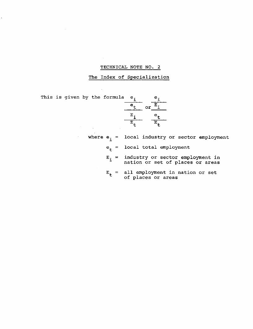
TECHNICAL NOTE NO. 2

The Index of Specialization

This is given by the formula e. e.

et or Ei

Ei tEt Et

where e. = local industry or sector employment1

et = local total employment

E. = industry or sector employment in1 nation or set of places or areas

E = all employment in nation or setof places or areas

TECHNICAL NOTE NO. 3

The Index of Surplus Employees

This is given by the formula S = el E et

E Et

where S represents the absolute number of "surplus" workersor employees in industry or sector (i). The upper limits ofthe index approaches e. asymptotically. The lower limitis et The index is useful as a general measure of

Et E

the basic quality of an industry or sector in an urbaneconomy. It is used here as a general indicator of "export"activity.

TECHNICAL NOTE NO. 4

The Definition of Urban Places

1. Many students of Mexican urban development haveargued that the census definition of urban population -2,500 - is unrealistic. Favoring a definition which regardsurban places as those with populations of 15,000 or 20,000,some have argued (Unikel and Torres: 1970) (Fox: 1968) thatpart of the so-called urban population captured by the censusis in fact rural - in economic and cultural terms. They havealso argued that the administrative map of Mexico reflectspast rather than present reality. There are, for example,571 municipios in Oaxaca but only 52 in Nuevo Leon, becauseOaxaca had a large indigenous population in the sixteenthcentury. Generally, the south of the country has moremunicipios than the north. Consequently, urbanization hasbeen more easily achieved in the south than the north, not-withstanding that the south is, in general, much lessdeveloped.

2. These are valid arguments which the mission respects.But in deciding to work with an urban definition correspond-ing to that of the census (2,500) several factors were weighedand,on balance, the counter arguments were more powerful.

3. First, there is the fundamental but unsettledquestion of the difference between "rural" and "urban".If the difference were economic, urban areas would, bydefinition, have no agricultural activities. If thedifference were cultural, urban areas would have a differentway of life. If the difference were a simple matter ofsize there is no reason that a nuclear population of 2,500people cannot be an urban population. On the other hand(Davis and Golden: 1953), it is argued that an urban nucleusbecomes more urban the larger it is.

4. These factors have led Unikel and Torres to proposea definition of urban places in Mexico which has a lowercut-off point of 20,000 - i.e., smaller populations are notconsidered urban at all. The "cities" thus defined havevery little agricultural activity and are almost entirelyconcerned with the properly "urban" functions of thesecondary and tertiary sectors.

5. The use of the urban municipio or urban censustract as a statistical base has certain conceptual advantages.If one is interested in urban change it is possible to measure -

as in this report - the process of urban change within thecensus tract over time by analyzing the changing structure of

economic activity - as revealed by employment data from oneyear to another. There is moreover no certainty that agri-culture may not be an urban activity in the sense that someof the economically active populations of large cities maywell tend to work outside the city. Moreover, from acultural standpoint there is less justification in I.atinAmerica - Mexico is no exception - for arguing that urbanways of life are markedly different from rural ways of life,that many migrants - to large cities in particular -- recreaterural ways of life in new urban environments (rurs in urbis)and that they may continue to live in a "rural" environmentlong after they have joined the urban population. 13ut, thenominally rural populations of areas proximate to cities areassociated with the city; they may even work there regularlyor occasionally and will probably visit more often thanthose who live beyond its immediate sphere of influence.

6. In short, any definition of what is "urban" andwhat is "rural" is arbitrary. While the mission found thecensus definition unsatisfactory on some grounds, i- alsofound reasons for accepting it.

7. The second question is methodological rather thanconceptual. Unikel and Torres have for 1940, 1950 and 1960,published data adjusting the urban census tracts to "cities",but their information concerns only urban population sizeand the economically active population. This report refersto many other chara-cteristics of urban population from popula-tion census data and other materials, notably those of theindustrial, commerce and service censuses, fiscal data,savings and loans data and many series of current statistics -all of which are available on a municipal base only. As apractical matter, the conversion of these data into a basesomething like Unikel's "cities" would have been impossibleeven if it had been unambigously desirable on conceptualground - which (for reasons already cited) was not the case.

8. Third, there was the question of the particularfocus of this report. The concern was with the past, presentand future of the country's major cities. We were thereforedealing with a set of urban places which in 1970 had more than100,000 people. Our interest in the general process ofurbanization was limited to the analysis of the framework ofurban size growth - in the country as a whole and on theregional level - as a background to the analysis of thedevelopment of the largest cities.

9. Finally, what difference does it make? The bestanswer is that at the national level the ratio of the urbanpopulation defined by the census to the urban populationas defined by Unikel falls from 1:1.20 in 1940 to 1:1.11in 1970.

10. These differences are not insignificant. The useof one or the other definition does not change the conclusionsabout urban development nor about other processes (includingindustrialization and economic growth). Nor does it changethe trends of the urban development process or produce adifferent rank order of cities in terms of any indicator ofurban development. In terms of results, it does not makemuch difference, but it does make more difference in someplaces than in others. For example, the urban population ofOaxaca in 1960 was 78,639 according to the municipal censustract and 75,196 according to Unikel, and the populationof Mexicali (the worst case of distortion) was 281,333according to the census and 179,539 according to Unikel.

11. No "correct" or fully satisfactory answer exists.That which has been given is believed to be defensible onconceptual grounds, unassailable on methodological grounds,reasonable in terms of the purpose for which it has beenused and pragmatically acceptable since it makes littledifference one way or the other.

12. Most of the analysis in this report thereforerefers to the municipal census tract. However, where it isfelt useful to introduce a different definition (most oftenthe 20,000 plus definition) this is done and the reasons areexplained. What is not done is to compare one definitiondirectly with another, although this has been done in atleast one recent paper (Unikel and Garza 1971).

TECHNICAL NOTE NO. 5

Population Growth Analysis

The 37 c:Lties were divided in six regions because(a) vital statistics and migration consist of estimates whichare subject to serious error, and grouping of municipalitiestherefore decreases the error factor, and (b) populationcharacteristics affect entire regions rather than individualcities or municipalities.

Three factors were taken into account (1) whethera state had experienced net inmigration or net outmigrationduring the previous three decades, (2) whether it hadexperienced a relatively high or a relatively low rate ofnatural increase during the last three decades, and (3)whether two or more states had common borders.

(1) Baja California, Colima, Morelos, NuevoLeon, and Sonora had net immigration andhigh rates of natural growth during allthree decades;

(2) Aguascalientes, Campeche, Coahuila, Durango,Queretaro, S.L.P., Tlaxcala and Zacatecashad high rates of natural growth but werenet outmigration states during the lastthree decades;

(3) The Federal District had net immigrationand a low rate of natural growth duringthe! three decades;

(4) Chiapas, Oaxaca, Puebla, and Veracruz hadlow rates of natural growth and net out-migration during the last three decades.

The other 14 states fell into different groups indifferent decades,, so it was decided to base the classificationon the situation in the last decade 1960-70. Thus:

(1) High natural growth - net immigration: BajaCa:lifornia, Baja California Territory, Sinaloa,andl'Tabasco;

-2-

(2) High natural growth - net outmigration;Chihuahua, Nayarit, Yucatan, Guanajuato,Guerrero, Michoacan, and Jalisco;

(3) Low natural growth - net immigration:Mexico, Quintana Roo, and Tamaulipas;

(4) Low natural growth - net outmigration:Hidalgo.

The following groups thus emerged:

(1) Baja California, Baja California Territory,Sonora and Sinaloa, all of which had a highrate of natural growth and net immigrationin the last decade;

(2) Chiapas, Oaxaca, Puebla, Veracruz, andHidalgo, all of which had a low rate ofnatural growth and net outmigration inthe last decade;

(3) Aguascalientes, Coahuila, Durango,Queretaro, S.L.P., Zacatecas, Chihuahua,Nayarit, Guanajuato, Guerrero, Michoacan,and Jalisco, all of which had a highrate of natural growth and net outmigrationduring the last decade;

(4) Mexico and Mexico City with net inmigrationand low rate of natural increase during thelast decade.

This left out the states of Tabasco, Morelos, NuevoLeon, Campeche, Tlaxcala, Yucatan, Quintana Roo, Tamaulipasand Colima.

Because of the number of states in group three itwas decided to divide that group by taking Guanajuato,Guerrero, Michoacan, and Jalisco away from it because oftheir geographic proximity and somewhat similar characteristicsin the three decades. Guanajuato, Michoacan, Guerrero, hadlow natural growth and outmigration in 1950-1960 while inthe other two decades these states had high natural growthrates and outmigration.

- 3 -

The states of Tabasco and Yucatan were added togroup 2 because of their geographic location. For t:he samereason Morelos was added to group 4.

Nuevo Leon and Tamaulipas were joined intc) a singlegroup because of their physical proximity.

In review the regions are as follows:

Region I: Mexico City, Mexico and Morelos 3

Region II: Jalisco, Guerrero, Michoacan,Guanajuato 4

Region III: Nuevo Leon, Tamaulipas 2

Region IV: Puebla, Yucatan, Veracruz,Tabasco, Oaxaca, and Hidalgo 6

Region V: Coahuila, Chihuahua, San LuisPotosi, Aguascalientes, Durango,Coahuila, and Queretaro, 7

Region VI: Baja California, Sonoro andSinaloa 3

25

The other seven states: Nayarit, Zacatecas, Campeche,Tlaxcala, Chiapas, and the Territories of Baja California andQuintana Roo were not assigned to any region because they didnot have cities of 100,000 or more population in 1970 andwere not important for this analysis.

TECHNICAL NOTE NO. 6

The Location Quotient

This was devised by Sargent Florence (1948). Itmeasures the degree to which a particular industry or sectoris concentrated in an area or place relative to the extentto which all activity is concentrated there - measured onthe basis of employment data.

It is given by the formula:

Numbers employed in industry orsector in place or area of totalin nation or set of places

Numbers employed in all industriesor sectors in place or area asshare of national total.

TECHNICAL NOTE NO. 7

Census Adjustments Relating to Employment inthe Services Sector

The major contrast between the 1960 and 1L970censuses in this regard refers to the transfer of certainactivities previously included in the industrial sector tothe services sector. The main category affected is work-shops and similar small establishments. The effect is toinflate the size of the services sector from one year tothe other.

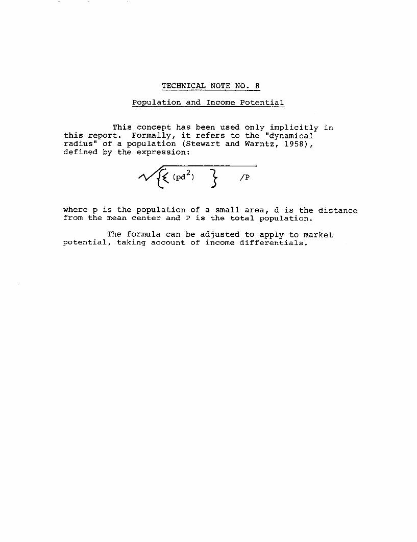
TECHNICAL NOTE NO. 8

Population and Income Potential

This concept has been used only implicitly inthis report. Formally, it refers to the "dynamicalradius" of a population (Stewart and Warntz, 1958),defined by the expression:

(pd2 ) } /P

where p is the population of a small area, d is the distancefrom the mean center and P is the total population.

The formula can be adjusted to apply to marketpotential, taking account of income differentials.

TECHNICAL NOTE NO. 9

The Beta Coefficient as an Index Connectivi-ty

This derives from graph theory. In a given net-work, connectivity rises as the number of "edges" increase,thus improving connectivity between the "vertices". Thatis: B1 no. of edges

no. of vertices'

="edges"

o = "vertex";

For example:

A B

B = 0.86 B = 1.00

C D

0 o _

B = 1.14 B =1.28