Urban Containment: The Social and Economic · PDF fileEven in the densest parts of urban areas—the ... Moving Cooler was strongly criticized by a sponsor, ... International data

by Wendell CoxProject Director: Dr. Adrian T. Moore

Reason FoundationPolicy Study No. 449

March 2016

Urban Containment: The Social and Economic Consequences of Limiting Housing and Travel Options

Reason FoundationReason Foundation’s mission is to advance a free society by developing, applying

and promoting libertarian principles, including individual liberty, free markets and

the rule of law. We use journalism and public policy research to influence the frame-

works and actions of policymakers, journalists and opinion leaders.

Reason Foundation’s nonpartisan public policy research promotes choice, compe-

tition and a dynamic market economy as the foundation for human dignity and

progress. Reason produces rigorous, peer-reviewed research and directly engages the

policy process, seeking strategies that emphasize cooperation, flexibility, local knowl-

edge and results. Through practical and innovative approaches to complex problems,

Reason seeks to change the way people think about issues, and promote policies that

allow and encourage individuals and voluntary institutions to flourish.

Reason Foundation is a tax-exempt research and education organization as defined

under IRS code 501(c)(3). Reason Foundation is supported by voluntary contribu-

tions from individuals, foundations and corporations. The views are those of the

author, not necessarily those of Reason Foundation or its trustees.

Copyright © 2016, Reason Foundation. All rights reserved.

R e a s o n F o u n d a t i o n

Urban Containment: The Social and Economic Consequences of Limiting Housing and Travel Options by Wendell Cox Project Director: Dr. Adrian T. Moore

Executive Summary Responding to a growing interest in curtailing carbon emissions, some cities are limiting their urban footprint—a practice called “urban containment.” Urban containment policy seeks to control “urban sprawl” and to reduce GHG emissions by densifying urban areas and substituting transit, cycling and walking for car and other light duty vehicle use. This study evaluates four urban containment reports—by the U.S. Department of Energy, the Transportation Research Board (Driving and the Built Environment), the Urban Land Institute (Moving Cooler) and the U.S. Environmental Protection Agency—to determine their cost-effectiveness in reducing greenhouse gas (GHG) emissions and their impact on household affluence and the poverty rate. Urban Containment and Cities Cities have experienced declining population densities for centuries. This occurred as urban areas expanded at a greater rate than population, due in large measure to improved transportation technologies, as walking was substantially replaced by transit and later, transit was substantially replaced by cars. Even in the densest parts of urban areas—the core municipalities—population densities have declined virtually around the world. The physical expansion of cities, known as “urban sprawl,” has been a principal concern of urban planners for decades, which has led to the adoption of “urban containment.” The most important urban containment policies are restrictions on urban fringe development—by means of urban growth boundaries or similar land-rationing measures—and policies to reduce light duty vehicle use.

Concern about GHG emissions drives an increasing emphasis on urban containment policy. This is based on the assumption that higher densities and less car use would translate into materially lower GHG emissions. In effect, urban containment policy seeks to replace the more liberal land-use policies that have been typical in U.S. metropolitan areas since World War II. Urban Containment and GHG Emissions The DOE report, which reviews other reports, indicates that urban containment policies “have significant potential to impact ... GHG emissions significantly over the long term.” The DOE report provides an overview of urban containment policy and summarizes GHG emissions reduction projections from previous research. The two most important reports reviewed—Driving and the Built Environment and Moving Cooler—indicate that urban containment policies could reduce 2050 greenhouse gas emissions from light duty vehicles by 1% to more than 10%. The later EPA report projected 2050 GHG emissions reductions at 4.3%. These projections raise several issues for analysis:

§ Driving and the Built Environment itself raises doubts about the political feasibility of implementing the policies the reports deem “necessary” to reduce GHG emissions.

§ Moving Cooler was strongly criticized by a sponsor, AASHTO (American Association of State Highway and Transportation Officials), which withdrew from the project indicating that the conclusions were based on “assumptions that are not plausible” and that the report “did not produce results upon which decision-makers can rely.”

§ Recent analysis casts further doubt on the potential for urban containment to reduce GHG emissions.

§ Comprehensive research at the University of California questions the robustness of the association between strategies to increase population densities and reducing GHG emissions.

In response to these uncertainties, this analysis examines and evaluates the range of projections from both Driving and the Built Environment (range minimum) and the EPA report (range maximum). This study finds that the overwhelming share of GHG emissions reduction projected in each of the reports is caused by fuel economy improvements from the base years that are assumed in the modeling, not urban containment policy. Since fuel economy is likely to continue to improve, even greater GHG emission reductions are likely in the near future. Moreover, this study contends that additional GHG emissions from the increased traffic congestion likely to be produced by the denser environments created by

urban containment policies could materially mitigate or even overwhelm the projected GHG emissions reductions projected in the reports. Finally, this study cautions that the use of long-term projections based on anticipated human behavioral changes is inherently unreliable, suggesting substantial margins of error. Moreover, the projected GHG emissions from urban containment policy are so small that they could be offset by projection errors and unreliability. Urban Containment and Mobility Economic growth in metropolitan areas is strongly associated with higher levels of mobility. Metropolitan areas are labor markets. If employees are able to access a larger percentage of jobs in a fixed period of time (such as 30 minutes), the economic productivity of the metropolitan area is likely to be greater. U.S. metropolitan areas rely principally on light duty vehicles for personal mobility. Transit access is very limited. On average, only 6% of jobs in major metropolitan areas can be reached on transit in 45 minutes by the average employee. In contrast, nearly two-thirds of jobs can be reached by light duty vehicle in that same time frame. Low transit use not only reflects reachability of employment but also quality of transportation mode. While transit works for some point-to-point downtown commuters, it is less effective for other trips, including non-work travel, which makes up nearly 85% of trips. This is because light duty vehicles offer a vastly speedier, less burdensome mode of transportation for all manner of non-commute trips, such as parents transporting children or pets, equipment or large or heavy items, groceries in need of refrigeration/freezing, or “trip-chaining” several errands. Higher densities are strongly associated with increased traffic congestion. This not only impedes personal mobility but is also a concern with respect to commercial traffic and business costs. Texas A&M Transportation Institute data indicate a strong relationship between limiting the expansion of roadways and greater traffic congestion over the last three decades. By favoring modes of transport (transit, cycling and walking) that cannot equal the mobility provided by light duty vehicles, urban containment could retard the productivity of metropolitan areas and significantly degrade people’s everyday lives, leading to a lower standard of living and greater poverty.

Urban Containment and Housing Affordability For much of the period since World War II, there has been comparatively little variation in house prices relative to household incomes around the country. However significant differences have arisen in more recent decades, in some places more than in others, and especially in dense, urban areas. Economic theory indicates that limits on supply tend to increase prices, all things being equal, regardless of the good or service (including land for housing). This potential association is largely dismissed by urban containment advocates and the DOE report, yet a considerable body of research confirms the economic theory that limiting the supply of a good (land) upsets the ratios between demand and supply, leading to higher prices (houses). The fundamental difficulty is that the “competitive supply of land” identified by economist Anthony Downs is not maintained. This study finds the expected correlation between higher house prices and limited land supply confirmed by the research. As early as 1973, British researchers were associating higher house prices with urban containment and especially noting negative effects on low-income households. A number of researchers have identified similar results across the United States and internationally. A study by the Tomas Rivera Institute in California expressed concern about the negative impacts on Hispanic and African American households. A detailed examination by Dartmouth economist William Fischel identified the land use regulatory structure as the principal reason for California’s extraordinary house price increases. An examination of housing affordability in Portland shows substantial price increases since the research cited in the DOE report, and particularly large increases in housing costs in high-density and low-income core areas. Housing is generally a household’s largest expenditure item, thus the variation in housing costs between metropolitan areas has a greater impact than that of other expenditure items. Therefore the higher house prices relative to incomes that are associated with urban containment reduce household discretionary income, leading to a lower standard of living and higher poverty rates. Urban Containment and GHG Emission Reduction Costs It is necessary to minimize the costs of any level of GHG emissions reductions to preserve economic growth and the standard of living. The normal metric for evaluating the cost of GHG emissions reduction is the cost per metric ton of carbon dioxide equivalent. Cost varies significantly between economic sectors, and it is important to select the most cost-effective strategies, regardless of economic sector. “Across-the-board” reductions can lead

to more-costly and less-effective strategies being implemented, which could threaten economic growth. The cost per metric ton of carbon dioxide equivalent emissions from urban containment policy is hundreds to thousands of times the cost of reducing emissions in the power sector. There are thus vastly more cost-effective alternatives to urban containment policy for reducing GHG emissions. Research by both the Congressional Budget Office and Resources for the Future found that sufficient GHG emission reductions can be achieved without reducing driving or living in denser housing. Urban Containment and the Broader Economy There are broader consequences to urban containment policy. Research has associated urban containment policy with slower metropolitan area employment growth and slower economic growth. Further, during the last decade there was a pronounced net domestic migration toward lower cost housing metropolitan areas from higher cost areas. With their restrictions on development outside the urban footprint, urban containment policies effectively trap people and businesses into higher cost areas, with unintended consequences for the broader economy. Urban Containment and the Standard of Living The United States has the most affluent metropolitan areas in the world, despite their low density. International data indicate that, compared to other nations, traffic congestion in the United States is less intense and average work trip travel times are better, indicating a higher level of mobility. International data also indicate that housing is generally more affordable relative to incomes than in other nations. Implementation of urban containment policies will likely lead to more-congested cities and less mobility, as well as lower discretionary incomes as house prices rise relative to incomes. The result would be a lower standard of living and greater poverty. Sufficient GHG emissions reductions can be achieved without urban containment policy and its attendant economic problems. The key is focusing on the most cost-effective strategies, without unnecessarily interfering with the dynamics that have produced the nation’s affluence.

R e a s o n F o u n d a t i o n

Table of Contents

Introduction ............................................................................................................ 1

Cities and Urban Containment ................................................................................. 2 A. Declining Urban Densities ............................................................................................... 2

1. Declining Overall Urban Area Densities ................................................................................... 2 B. Description of Urban Containment Policy ......................................................................... 3

1. Increase Population Densities ................................................................................................. 4 2. Promote Transit, Cycling and Walking ..................................................................................... 4

C. Impetus for Urban Containment Policy ............................................................................. 4

Urban Containment and GHG Emissions ................................................................... 6 A. Projected GHG Emissions Reductions .............................................................................. 6

1. Driving and the Built Environment ........................................................................................... 6 2. Moving Cooler ....................................................................................................................... 6 3. The EPA Report ....................................................................................................................... 7 4. The DOE Report ....................................................................................................................... 7

B. Analysis of Issues Raised by the Four Reports .................................................................. 8 1. Traffic Congestion and GHG Emissions .................................................................................... 8 2. Scale of Urban Containment GHG Emissions ........................................................................... 9 3. New Fuel Economy Standards ................................................................................................ 10 4. Technical and Objectivity Problems in Assessing GHG Emission Reductions ............................ 11

C. Density Increases and Household GHG Emissions Reductions ......................................... 12 D. Assessment: Urban Containment and GHG Emissions ..................................................... 13

Urban Containment and Mobility in Metropolitan Areas .......................................... 15 A. Mobility and Access ....................................................................................................... 15 B. The Role of Transit and Light Duty Vehicles ..................................................................... 16

1. Transit and Light Duty Vehicle Access .................................................................................... 17 2. Mobility for Low-Income Households .................................................................................... 20

C. Higher Densities and Traffic Congestion ......................................................................... 21 1. Roadway Capacity and Traffic Congestion .............................................................................. 22

D. Urban Containment and Mobility .................................................................................... 23 E. Assessment: Urban Containment and Mobility in Metropolitan Areas .............................. 24

Urban Containment and Housing Affordability ........................................................ 25 A. Housing Affordability: Historical Context ........................................................................ 25 B. Housing Affordability and the Urban Containment Reports ............................................. 26 C. Urban Containment and Housing Affordability: The Research .......................................... 27

1. International Research ......................................................................................................... 28 2. Greater Attraction of Property Investors (also referred to as “speculators”) ............................ 29 3. Detrimental Impact on Minority and Lower Income Households ............................................. 29

D. Urban Containment and Housing Affordability: The Experience ....................................... 30

1. Housing Affordability in California ......................................................................................... 30 2. Housing Affordability in Portland ............................................................................................ 31

E. Potential Impact on Home Ownership ............................................................................. 36 F. Assessment: Urban Containment and Housing Affordability .............................................. 37

Urban Containment and GHG Emission Reduction Costs .......................................... 38 A. Reducing GHG Emissions Cost-Effectively ....................................................................... 38 B. Mobility and the Cost of GHG Emissions Reductions ....................................................... 39 C. Housing Affordability and the Cost of GHG Emissions Reductions .................................... 40 D. Assessment: Urban Containment and GHG Emission Reduction Costs ............................. 40

Urban Containment and the Broader Economy ......................................................... 41 A. Assessment: Urban Containment and the Broader Economy ............................................ 42

Urban Containment and the Standard of Living ........................................................ 43 A. America’s Affluent Metropolitan Areas ............................................................................ 43 B. Maintaining the Standard of Living ................................................................................. 44 C. Assessment: Urban Containment and the Standard of Living ........................................... 44

Conclusion ............................................................................................................. 45

About the Author .................................................................................................... 47

Endnotes ............................................................................................................... 48

Urban Containment | 1

P a r t 1

Introduction

Responding to a growing interest in curtailing carbon emissions, many cities are limiting their urban footprint—a practice called “urban containment.” Urban containment policy seeks to control the spatial expansion of cities, or “urban sprawl,”1 and to reduce greenhouse gas (GHG) emissions by densifying urban areas and transferring urban travel demand from cars, light trucks and sport utility vehicles (collectively called “light duty vehicles”) to transit, cycling and walking. This philosophy now dominates urban planning in the United States. But urban containment policies do far more than change transportation modes. They affect personal mobility, housing affordability, the broader economy and the standard of living. To assess urban containment policies’ effect on the environment, this study evaluates four reports that examine the potential for reducing urban transportation GHG emissions using urban containment policy. These reports were published by the U.S. Department of Energy (the DOE report), the Transportation Research Board (Driving and the Built Environment), the Urban Land Institute (Moving Cooler) and the U.S. Environmental Protection Agency (the EPA report). This study evaluates them for cost-effectiveness of urban containment’s GHG emission reduction strategies and the impact on household affluence, poverty, mobility, housing, the economy and standards of living.

2 | Reason Foundation

P a r t 2

Cities and Urban Containment

As transportation technologies have improved, the built-up urban areas of cities2 have declined in population density. The “walking” cities of the 18th century and before had far higher population densities than current cities. During the 19th century, growth was stronger in lower density districts of the urban areas, and some urban core districts lost population.3 This was facilitated by advances in mass transit that made it possible for people to commute greater distances. The advent of the automobile fostered a further decline in densities as it became nearly universal in its availability. In addition, both transit and light duty vehicles materially expanded the geographic scope of mobility for residents within cities.

A. Declining Urban Densities Even the densest parts of metropolitan areas, the core municipalities known as “central cities,” have generally become less dense in recent decades. Among more than 70 core municipalities in the high-income world that were fully developed in 1950 and have not materially added to their boundaries, only one added population between the 1950s and the early 2000s.4 Population declined not only in U.S. core municipalities, but also in large international core municipalities, such as Paris (20%), the former London County Council area (30%), Copenhagen (30%), Milan (30%) and Seoul (nearly 10%).5 Over the past decade, however, there has been a population resurgence in U.S. city cores, reversing decades of decline. Yet the increase in population that occurred within two miles of the city halls of historical core municipalities between 2000 and 2010 was more than offset by a decline in the ring between two miles and five miles from city hall.6

1. Declining Overall Urban Area Densities Moreover, even as urban areas have become larger, they have become less dense, because the spatial expansion has been greater than the population increase. This is the case in the lower income world as well.7


For example, the New York City built-up urban area (as opposed to the core municipality) added more than 50% to its population between 1950 and 2010, yet its urban land area nearly tripled and its population density declined more than 45%.8 Each of New York City’s three densest boroughs has lost population since 1950. The nearby Philadelphia urban area has seen its density drop 70% over the same period of time, while the population has increased 85%, indicating a very large urban spatial expansion.9 Internationally, historic data are sparse, but show a decline in urban densities over the past few decades.10 For example, the Paris urban area, whose population increased 40% since the 1960s, has experienced a population density loss of nearly 30% since then. The current urban density of Paris is approximately one-tenth that of the early 19th century.11 In the U.S. and internationally, while the urban core losses have been facilitated by transportation improvements, higher incomes and smaller household sizes have also contributed to the trend.

B. Description of Urban Containment Policy Cities (metropolitan areas or urban areas) are the context of urban containment policy. The continuing geographical expansion of cities has concerned urban planners for decades. Early on, they feared that urbanization consumed too much agricultural land and threatened the food supply.12 As a result, planners developed urban containment policy, also known as “smart growth,” “densification,” “growth management,” “compact cities” and “livability.” Urban containment policy seeks to restrict the spatial or geographic growth of cities, while attempting to attract people out of cars and onto transit, walking and bicycles.

Urban containment has two fundamental purposes: (1) to promote compact and contiguous development patterns that can be efficiently served by public services and (2) to preserve open space, agricultural land, and environmentally sensitive areas that are not currently suitable for urban development.13

Urban containment generally includes legally mandated strategies to increase urban population densities, such as reducing the “greenfield” land than can be developed and encouraging building in “brownfield” or already developed areas. Related policies restrict the roadway capacity improvements that would match increasing travel demand.


1. Increase Population Densities Various urban containment strategies seek to increase urban population densities. Perhaps the most important urban containment strategy is the urban growth boundary14 that is drawn around urban areas. New development is discouraged or even outlawed outside an urban growth boundary.

In its most basic form, urban containment involves drawing a line around an urban area. Urban development is steered to the area inside the line and discouraged (if not prevented) outside it.15

The most notable U.S. cases of urban growth boundaries are in Portland (Oregon), Seattle, Miami, Denver, Washington, D.C., Los Angeles, San Francisco, San Diego and San Jose. In some cases, such as the Washington, D.C. metropolitan area, the California metropolitan areas and Miami, the urban growth boundaries have been adopted at the county or municipal level. There are substantial variations between urban growth boundary policies, not only in substance but also in flexibility and enforcement. Urban growth boundaries are referred to by other terms, such as greenbelts, urban service areas, urban limit lines and agricultural preserves. Virtual urban growth boundaries can be created by large lot zoning on the urban periphery. Other related policies can also severely restrict the land on which new building can occur. In some places, policies require a certain percentage of new housing to be brownfield or infill (in the already developed areas), which can also prevent land development on the urban fringe.

2. Promote Transit, Cycling and Walking Urban containment policy favors mass transit, cycling and walking, and discourages automobile use in metropolitan areas. As a result, little or no new road capacity is provided. It is assumed that by discouraging automobile use and substituting travel by transit, walking and cycling, there will be a material reduction in GHG emissions.

C. Impetus for Urban Containment Policy Interest in urban containment policy has increased as concerns about greenhouse gas emissions have increased. The belief is that significant greenhouse gas emissions reductions can be obtained from forcing new development to remain within existing urban footprints, which it is presumed would reduce greenhouse gas emissions through shorter car trips and by transferring travel demand to transit, cycling and walking.


Proponents consider the imposition of urban containment so compelling that they seek to marginalize the more traditional, liberal land use planning that was typical following World War II. While most major U.S. metropolitan areas have not yet adopted strong urban containment policies, the urban planning community is pressuring to apply them throughout the nation. More than 100 metropolitan areas have implemented some form of urban containment policy.16


P a r t 3

Urban Containment and GHG Emissions

A. Projected GHG Emissions Reductions Four major reports published over the last six years by the U.S. Department of Energy, the Transportation Research Board, the Urban Land Institute and the Environmental Protection Agency analyze GHG emissions reduction as a result of urban containment policy. They represent the most prominent sources of support for urban containment policies as a means of addressing GHG emissions. Each of the four reviewed reports generally finds what it deems to be substantial potential to reduce greenhouse gas emissions from driving using urban containment policy.

1. Driving and the Built Environment This report was conducted by the Transportation Research Board of the National Academy of Sciences and published in 2009. It projects results for greenhouse gas emissions from urban containment policies under two different levels of densification.17 Its lower density scenario estimates greenhouse gas emissions from light duty vehicles would range from 1.3% to 1.7% (midpoint 1.5%) in 2050. The report also projects 8.4% to 11.0% (midpoint 9.7%) GHG emission reductions in 2050 in the higher densification scenario. These reductions are relative to a 2050 business-as-usual projection. Little of the reduction from a base year (2000) is from urban containment policies, with most of the reduction due to improved fuel economy.

2. Moving Cooler This report18 was published in 2009 by the Urban Land Institute. Moving Cooler examined three scenarios that would require 43%, 64% or 90% of future development to be in the densest portions of urban areas.19 In relation to total surface transportation GHG emissions, Moving Cooler projected a range of reductions from 1.2% to 6.7% from its 2050


baseline.20 Again, little of the reduction from a base year (2005) is from urban containment policies, with most of the reduction due to improved fuel economy (Table 1).

Table 1: Description of GHG Reductions: Moving Cooler and Driving and the Built Environment (GHG in millions of metric tons)

Moving Cooler Driving and the Built Environment*

43% Densification

Scenario

64% Densification

Scenario

90% Densification

Scenario

25% Densification

Scenario

75% Densification

Scenario Base Year 2005 2005 2005 2000 2000 Base Year GHGs 1,302 1,302 1,302 1,006 1,006 2050 Baseline GHGs 1,653 1,653 1,653 1,017 1,058 Urban Containment Impacts (20) (61) (110) (15) (103) Net GHGs 1,633 1,592 1,543 1,002 955 GHG Reduction 1.2% 3.7% 6.7% 1.5% 9.7%

* Driving and the Built Environment scenarios at midpoints

Source: Data from Moving Cooler and Driving and the Built Environment

3. The EPA Report This report, commissioned by the Environmental Protection Agency, projects greenhouse gas emission reductions over the period of 2009 to 2050 from a synthesis of plans by the regional planning organizations (metropolitan planning organizations).21 The EPA report’s urban containment strategies were projected to reduce greenhouse gas emissions from light duty vehicles by 4.3% in 2050 (relative to a 2050 business-as-usual projection that includes a substantial improvement in fuel economy, which is beyond the results projected from the urban containment strategies).22

4. The DOE Report The DOE report provides an overview of urban containment policy and summarizes GHG emissions reduction projections from previous research. From this analysis, the DOE report provides an estimate of the potential for urban containment policy to reduce greenhouse gas emissions, concluding that:

Although researchers still disagree on the extent to which land use accounts for differences in travel behavior among neighborhoods and regions, the evidence suggests that changes to the built environment, such as higher densities and mixed-use, walkable communities, have significant potential to impact transportation energy and GHG emissions significantly over the long term.23

The DOE report indicates that urban containment strategies are being implemented around the country, but that additional strategies could require strong “pricing or regulatory”


incentives to overcome “issues of public acceptance and related challenges in changing behavior.”

B. Analysis of Issues Raised by the Four Reports

1. Traffic Congestion and GHG Emissions As increasing traffic congestion impedes the free flow of traffic, light duty vehicles slow down and burn more fuel for each mile traveled. This results in a correspondingly higher level of GHG emissions (Figure 1).

Figure 1: Traffic Congestion and GHG Emissions (CO2 Grams/Mile)

Source: Transport Canada, The Cost of Urban Congestion in Canada, 2006, http://www.adec-inc.ca/pdf/02-rapport/cong-canada-ang.pdf

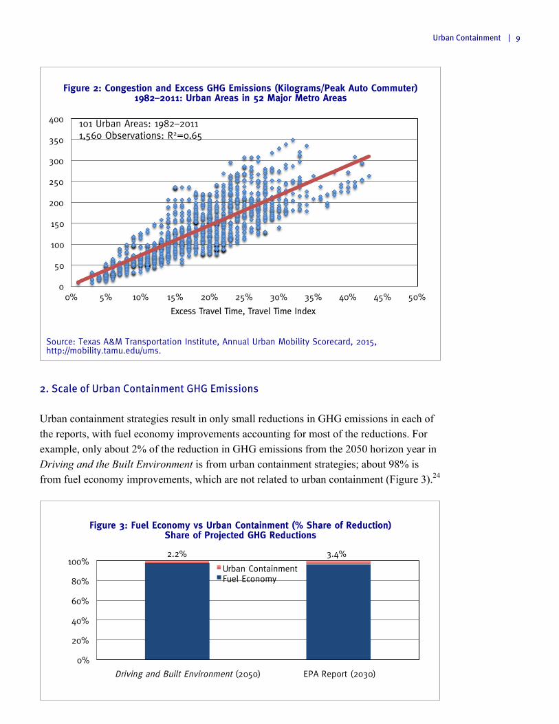
According to the Texas A&M Transportation Institute, excess GHG emissions attributable to traffic congestion rose substantially between 1982 and 2011, in close association with the increase in traffic congestion (Figure 2). As noted above, urban containment policy seeks to severely limit the expansion of roadway capacity. This, combined with the increase in traffic congestion associated with higher densities, is likely to result in an even greater increase in excess GHG emissions to 2040. The GHG emission increases from traffic congestion could neutralize or even overwhelm the anticipated small reductions that would be expected from urban containment policies.

0

100

200

300

400

500

600

Free Flow Congested

Freeway Arterial


Figure 2: Congestion and Excess GHG Emissions (Kilograms/Peak Auto Commuter)

1982–2011: Urban Areas in 52 Major Metro Areas

Source: Texas A&M Transportation Institute, Annual Urban Mobility Scorecard, 2015, http://mobility.tamu.edu/ums.

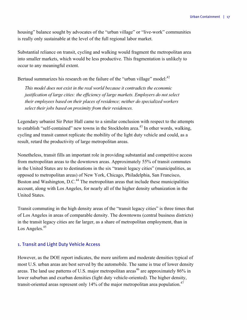
2. Scale of Urban Containment GHG Emissions Urban containment strategies result in only small reductions in GHG emissions in each of the reports, with fuel economy improvements accounting for most of the reductions. For example, only about 2% of the reduction in GHG emissions from the 2050 horizon year in Driving and the Built Environment is from urban containment strategies; about 98% is from fuel economy improvements, which are not related to urban containment (Figure 3).24

Figure 3: Fuel Economy vs Urban Containment (% Share of Reduction) Share of Projected GHG Reductions

0

50

100

150

200

250

300

350

400

0% 5% 10% 15% 20% 25% 30% 35% 40% 45% 50%

Excess Travel Time, Travel Time Index

101 Urban Areas: 1982–2011 1,560 Observations: R2=0.65

2.2% 3.4%

0%

20%

40%

60%

80%

100% Urban Containment Fuel Economy

Driving and Built Environment (2050) EPA Report (2030)


3. New Fuel Economy Standards

In recent years, U.S. Department of Energy Information Administration (EIA) projections of long-term GHG emissions25 from light duty vehicles have been revised downward as more-stringent fuel economy standards have been adopted. Between the 2008 projections and the early 2014 projections, the gross projected 2030 greenhouse gas emissions from light duty vehicles declined substantially—32%—from the actual 2005 estimate. The latest projections from EIA indicate a reduction of more than 50% below the level of GHG emissions from light duty vehicles that would have occurred if fuel economy had remained at the level projected in 2005 (Figure 4). While we cannot know or calculate which technologies will develop in the future to increase fuel economy, this revision shows that continued GHG emission reductions from improved fuel economy technologies are likely to continue.

The greenhouse gas emission reductions from fuel economy could be even greater in the longer run. The Department of Energy projections assume the same new vehicle fuel economy standards for every year after 2025. The result is that greenhouse gas emissions are reduced at a somewhat slower rate after 2025. It seems likely that there will be further improvements in light duty vehicle fuel economy between 2025 and 2040, such as from electric cars, fuel cell vehicles or other advanced technologies.26 By 2040, the greenhouse gas emissions reductions from fuel economy improvements alone are projected to be many times the reductions projected from urban containment (Figure 5).

Figure 4: Revised Light Vehicle GHG Projections (in Billion Annual Tons) 2005–2030 Gross National Emissions

Source: U.S. Department of Energy Information Administration, Annual Energy Outlook 2015, http://www.eia.gov/forecasts/aeo

0.0

0.2

0.4

0.6

0.8

1.0

1.2

1.4

1.6

1.8

2005 2030 As Projected in Year Noted Actual

As projected in AEO 2005




Figure 5: Light Vehicle GHG Reduction Projections (% Change)

Gross Emissions: Annual Reduction to 2040

4. Technical and Objectivity Problems in Assessing GHG Emission Reductions Leading experts, organizations and the reports themselves raise doubts about the high-end GHG emissions projections of Driving and the Built Environment and Moving Cooler. Moving Cooler’s principal sponsor, the American Association of State Highway and Transportation Officials (AASHTO), sharply criticized the project and withdrew from it over technical and objectivity concerns. AASHTO indicated that Moving Cooler associated unrealistic GHG reductions with its strategies and underestimated the potential for more fuel-efficient cars, telecommuting, ridesharing and improved transportation operations. According to AASHTO, Moving Cooler “did not produce results upon which decision-makers can rely.” AASHTO researchers further said that Moving Cooler relied on “assumptions that are not plausible,” and analysis that was “flawed and incomplete,” costs that were “incomplete and misleading,” projected greenhouse gas emission results that were “not comparable or plausible” and contained “many assumptions” that were “extreme, unrealistic and in some cases, downright impossible.” AASHTO dismissed Moving Cooler because its “heroic assumptions about land use and travel behavior and extraordinary pricing do not come close to the GHG reductions needed by 2050.”27 Another critique by Commuting in America author Alan Pisarksi made similar points.28

-1.52%

-0.03% -0.09%

-1.6%

-1.4%

-1.2%

-1.0%

-0.8%

-0.6%

-0.4%

-0.2%

0.0%

Fuel Economy

Other

Estimated from Driving and the Built Environment

Estimated from EPA Report

Fuel Economy (Estimated from DOE

Annual Energy Outlook)


Driving and the Built Environment itself indicates that some of the drafters questioned the plausibility of its higher density scenario due to the dramatic changes in “housing trends,” “land use policies” and “public preferences” required.29 Further, the projected GHG emission reductions are not from a contemporary base year, but are rather from a 2050 baseline that is projected to have increased GHG emissions, which may not be accurate. But even so, much of the reduction from the future baseline is the result of fuel economy improvements, not from urban containment policy, which is not reflected in the report (Table 2).

Table 2: GHG Reductions from Urban Containment and Fuel Economy (GHG in millions of metric tons)

Moving Cooler Driving and the Built Environment*

43% Densification

Scenario

64% Densification

Scenario

90% Densification

Scenario

25% Densification

Scenario

75% Densification

Scenario 2050 Baseline GHGs 1,653 1,653 1,653 1,017 1,058 2050 Baseline at Base Year Fuel Economy

3,446 3,446 3,446 1,690 1,613

Urban Containment Impacts (20) (61) (110) (15) (103) Fuel Economy Impacts (1,793) (1,793) (1,793) (673) (555) Total GHG Reduction (1,813) (1,854) (1,903) (688) (658) % from Urban Containment 1.1% 3.3% 5.8% 2.2% 15.6% % from Fuel Economy 98.9% 96.7% 94.2% 97.8% 84.4%

*Driving and the Built Environment scenarios at midpoints

Source: Data from Moving Cooler and Driving and the Built Environment

The DOE report indicated that in Driving and the Built Environment and Moving Cooler: “The higher end of the range is based on very optimistic assumptions…” and also noted that the authors of the two reports considered the “lower ranges ... to be more likely or feasible.”30 Other research cited in the DOE report suggests even greater greenhouse gas emission reductions. Given the caveats noted above with respect to the higher scenario projections in Driving and the Built Environment and Moving Cooler, and the uncertainties of behavioral modeling, these more aggressive projections could be highly speculative.31 A more plausible upper limit may be found in the EPA report. This suggests a range of 2050 GHG emission reductions due to urban containment policies from a low of 1.5% in Driving and the Built Environment to a high of 4.3% in the EPA report.

C. Density Increases and Household GHG Emissions Reductions GHG emissions are also produced by many sources other than light duty vehicles. Households use fossil fuels to heat and air condition their homes, and fossil fuels are also expended in the building of houses. Urban containment policies also affect U.S. household GHG emissions.


In perhaps the most comprehensive U.S. review of GHG emissions at the local level (zip code-level data), researchers at the University of California, Berkeley found no demonstrable potential for GHG reductions from urban containment policy in cities or suburbs: “Generally” there is “... no evidence for net GHG benefits of population density in urban cores or suburbs when considering effects on entire metropolitan areas.”32 According to this study:

Given these limitations of urban planning our data suggest that an entirely new approach of highly tailored, community scale carbon management is urgently needed. Regions with high energy-related emissions, such as the Midwest, the South, and parts of the Northeast, should focus more on reducing household energy consumption than regions with relatively clean sources of energy, such as California.

With respect to the suburbs, which urban containment policy seeks most to alter, the research indicates strong potential for GHG emission reductions through policies that would improve the fuel efficiency of vehicles and electric power consumption, rather than through densification initiatives:

Suburbs, which account for 50% of total U.S. HCF [human carbon footprint], tend to have high motor vehicle emissions, large homes, and high incomes. These locations are ideal candidates for a combination of energy efficient technologies, including whole home energy upgrades and solar photovoltaic systems combined with electric vehicles.

Despite the large share of GHG emissions it attributed to suburbs, this study found that a 1,000% density increase would produce only a 25% reduction in GHG emissions from less vehicle use and housing strategies. Thus, these findings are in opposition to the view that urban containment, with its objective of higher densities, has substantial potential to reduce GHG emissions.

D. Assessment: Urban Containment and GHG Emissions Urban containment seeks to densify cities so as to reduce GHG emissions, but disregards the fact that traffic congestion significantly increases GHG emissions. The increased emissions due to traffic congestion caused by urban containment are likely to overwhelm any emissions reductions gained from urban containment. The four analyzed reports advocate the use of urban containment to decrease GHG emissions, and yet they show those reductions to be dwarfed by the GHG emission reductions projected for greater fuel economy. Indeed, the projected reductions in GHG


emissions from urban containment policies are so small that they could be substantially negated by the margins of error of the forecasts. Increases in fuel economy have reduced GHG emissions significantly and will continue to do so in the future. While these reports cannot, and do not, predict unknown future improvements in fuel efficiency, such gains are likely to occur as technology becomes increasingly sophisticated. In fact, predictions of future GHG emissions made just 10 years ago have had to be adjusted downward as the cumulative effects of increased fuel efficiency and less driving have reduced greenhouse gases more than anticipated. While urban containment policies focus on reducing GHG emissions through decreased travel due to forced population density, they do not adequately address the contribution to GHG emissions made by household energy use. Since the reports themselves show that urban containment’s reduction of GHG emissions is slight at best, more impact is likely to come from addressing household energy use, primarily electricity, to reduce GHG emissions. While fuel economy can be calculated with some accuracy, predicting changes in behavior is riskier. The flexibility and autonomy attained through the rise of the automobile has made it the preferred choice for the vast majority of people. Compelling people to change their preferences through enforced densely packed urban settings, and then making calculations based on predictions of human behavior in that setting over four or five decades is simply too unreliable. The four reports themselves call their own calculations of predictions of GHG emission reduction into question, and loosely based assumptions even caused one sponsor to leave a project. The state of modeling is not sufficiently advanced to produce reliable projections, given so much uncertainty.


P a r t 4

Urban Containment and Mobility in Metropolitan Areas

A. Mobility and Access Mobility involves the ability to rapidly access destinations throughout a city. The economic literature generally associates stronger urban area economic growth and job creation with the ability of workers to access the maximum number of jobs in a short travel time. For decades this assumption has been a principle of transport planning. Projects are routinely evaluated, at least in part, based on the amount of time that they will save users. In 1998, researchers examined the productivity of cities in relation to employment access, establishing that the “effective” labor market is defined both in terms of employers and employees and measured by the number of jobs in the metropolitan area that can either:

(1) Be accessed in a particular period of time (such as 30 minutes) by workers (the employee point of view), or

(2) Be accessed by the labor force in relation to the work location (the enterprise point of view).33

Further studies indicated a strong relationship between higher journey-to-work travel speeds and employee productivity:34

… average commute speed—reflecting the provision of transportation infrastructure—most strongly influenced labor productivity in the San Francisco Bay Area, with an elasticity of around 0.10—every 10% increase in commuting speed was associated with a one percent increase in worker output, all else being equal.

Similar results were indicated in research on U.S. urban areas published by Reason Foundation.35


Higher densities as are sought by urban containment policies result in generally slower work trip travel times. Hong Kong may be the ultimate in urban containment cities. With an urban population density of 68,000 per square mile, Hong Kong is 10 times as dense as Los Angeles and nearly 20 times as dense as Portland, Oregon.36 As a result, Hong Kong has a high employment density. It also has one of the highest transit work trip market shares in the world. The average work trip is only 4.8 miles long, less than one half the U.S. average of 11.8 miles, yet Hong Kong’s average one-way work trip travel time is 47 minutes,37 the longest reported in the high-income world.38 As illustrated by this example, and supported by copious research, higher population densities are associated with longer work trip travel times.39

B. The Role of Transit and Light Duty Vehicles Metropolitan areas are labor markets. According to former World Bank principal planner Alain Bertaud:40

The welfare of cities is dependent on their labor markets. The larger the market, the more innovative and productive the city, as long as labor markets do not fragment into smaller adjacent markets as they grow. Maintaining mobility is therefore essential to the economic viability of cities.

Urban containment policy favors the fragmented markets described above. It seeks to transfer urban travel demand from automobiles to transit, cycling and walking, at least in part through higher population densities. A principal strategy is to establish “transit-oriented developments,” or “urban villages” in which planners intend for people to live and work, use their cars minimally and travel by transit, cycling or walking. Researchers Angel and Blei describe this as the “live-work” model.41

This model, in its pure and ideal form, views metropolitan areas as a set of small, discrete and self-contained economies, so to speak, with all commuting trips taking place within them and no commuting trips taking place between them.

The purpose of such communities is to substantially reduce the use of automobiles, which would be accomplished by people living close enough to their jobs and shopping to walk, use bicycles or use transit. In fact, however, in the modern metropolitan area (the labor market), people travel much farther than is possible by walking or bicycles, and they go to locations not accessible by transit, both to work at the jobs that best suit them and to obtain the best prices. The “jobs-


housing” balance sought by advocates of the “urban village” or “live-work” communities is really only sustainable at the level of the full regional labor market. Substantial reliance on transit, cycling and walking would fragment the metropolitan area into smaller markets, which would be less productive. This fragmentation is unlikely to occur to any meaningful extent. Bertaud summarizes his research on the failure of the “urban village” model:42

This model does not exist in the real world because it contradicts the economic justification of large cities: the efficiency of large markets. Employers do not select their employees based on their places of residence; neither do specialized workers select their jobs based on proximity from their residences.

Legendary urbanist Sir Peter Hall came to a similar conclusion with respect to the attempts to establish “self-contained” new towns in the Stockholm area.43 In other words, walking, cycling and transit cannot replicate the mobility of the light duty vehicle and could, as a result, retard the productivity of large metropolitan areas. Nonetheless, transit fills an important role in providing substantial and competitive access from metropolitan areas to the downtown areas. Approximately 55% of transit commutes in the United States are to destinations in the six “transit legacy cities” (municipalities, as opposed to metropolitan areas) of New York, Chicago, Philadelphia, San Francisco, Boston and Washington, D.C.44 The metropolitan areas that include these municipalities account, along with Los Angeles, for nearly all of the higher density urbanization in the United States. Transit commuting in the high density areas of the “transit legacy cities” is three times that of Los Angeles in areas of comparable density. The downtowns (central business districts) in the transit legacy cities are far larger, as a share of metropolitan employment, than in Los Angeles.45

1. Transit and Light Duty Vehicle Access However, as the DOE report indicates, the more uniform and moderate densities typical of most U.S. urban areas are best served by the automobile. The same is true of lower density areas. The land use patterns of U.S. major metropolitan areas46 are approximately 86% in lower suburban and exurban densities (light duty vehicle-oriented). The higher density, transit-oriented areas represent only 14% of the major metropolitan area population.47


For the great majority of urban trips, transit is not a substitute for light duty vehicle travel, because it does not connect most origins and destinations in travel times that are competitive with light duty vehicles. In 2010, the average single occupant light duty vehicle commute was approximately one-half as long as the average transit commute (24.0 minutes compared to 47.4 minutes).48 Virtually everywhere in the nation, door-to-door work trip travel times are longer by transit than by light duty vehicles.49 Some planning agencies use access to transit to evaluate the effectiveness of transit systems. Brookings Institution data show that 85% of employees live within walking distance of a transit station or stop in the 10 metropolitan areas with the largest share of population living at 10,000 per square mile or greater density (Figure 6). Yet, those50 data also show that an average of only 7% of the jobs in major metropolitan areas can be reached from the residences of the average employee in 45 minutes or less.51 This is approximately 20 minutes longer than the average light duty vehicle commute time. Thus, it can be concluded that, on average, a commuter has a less than 10% chance of reaching a job from a nearby transit stop (7% divided by 85%). Having good access to transit does not mean good access to jobs throughout the metropolitan area (Figure 7). Outside of jobs in larger downtown areas, virtually all of which were developed before World War II, transit provides comparatively little job access to the rest of the metropolitan area. Light duty vehicles provide considerably more access than transit. Research indicates that, on average, 65% of jobs in the major metropolitan areas are accessible in 30 minutes or less by light duty vehicle to the average employee in the major metropolitan areas.52 It would be a prohibitively expensive project to expand transit service sufficiently to equal automobile access. Research suggests that it could take as much as all of the personal income of a major metropolitan area each year to provide such service.53 Walking and bicycles are inherently more limited than cars in their geographical access to employment in metropolitan areas, and in inclement weather provide a low-quality commute. Among current technologies, the automobile cannot be equaled in the mobility it provides throughout the metropolitan area.


Figure 6: Transit Access in 45 Minutes: Average Employee Major U.S. Metropolitan Areas with Most >10,000 Density*

Source: Brookings Institution: Missed Opportunity 2012.

www.brookings.edu?~/media/research/files/reports/2011/5/12-jobs-and-transit/0512_jobs_transit.pdf *Most >10,000 density: Largest population living at densities at above 10,000 per square mile.

Figure 7: Transit Job Access: Average Employee Metropolitan Areas with Most >10,000 Density*

*Most >10,000 density" means the 10 metropolitan areas with the largest share of population living at 10,000 per square mile or greater density. Source: Brookings Institution: Missed Opportunity 2012

Transit stop nearby, jobs not

within 45 minutes

78%

Transit stop nearby: jobs within 45 minutes

7%

Transit stop not nearby, jobs cannot be

accessed by transit 15%

0% 10% 20% 30% 40% 50% 60% 70% 80% 90% 100%

San Diego

San Jose

Miami

Washington

Boston

Philadelphia

San Francisco-Oakland

Chicago

Los Angeles

New York

Transit stop nearby: jobs within 45 minutes

Transit stop nearby, jobs not within 45 minutes

Transit stop not nearby, jobs cannot be accessed by transit


2. Mobility for Low-Income Households Research has noted the importance of automobile access to lower income workers:54

Even in cities with good transit service, transit travel times, on average, far exceed automobile travel times because of walking to and from stops, waits at stops and for transfers, and frequent vehicle stops along the way. These slower travel speeds are especially difficult for parents who must “trip chain,” make stops for child care or shop along the commute.

This research suggested that:

Given the strong connection between cars and employment outcomes, auto ownership programs may be one of the more promising options and one worthy of expansion.

And further that:

Those workers fortunate to have access to automobiles can reach many employment opportunities within a reasonable commute time regardless of where they live.

This study finds substantial advantages in employment outcomes for people with cars as compared to those without cars.55 Other research shows that access to automobiles can substantially reduce rates of unemployment for lower income African-American workers.56 In a study of transit mobility in Atlanta, Baltimore, Dallas, Denver, Milwaukee and Portland, researchers found that transit had “virtually no association with the employment outcomes” of welfare recipients.57 The problem is that transit’s travel times and its geographic access limitations severely impair its ability to provide mobility throughout the metropolitan area for low-income households. Despite the general assumption that low-income households depend on transit for their mobility, the car plays a pivotal role. This may be caused, at least in part, by the limited geographical and time mobility of transit. According to American Community Survey data, 76% of low-income workers commute by car, a figure nearly as high as the overall average of 83%.58 The social implications of better mobility are suggested by researcher Alan Pisarski, who observed that automobile-based transport systems have “democratized” mobility.59 The automobile has made it possible to access entire metropolitan areas and their widely dispersed employment and shopping at comparatively low cost. While the economic impact of improved employment mobility that the automobile facilitates has contributed substantially to job creation and economic growth, the travel impact has been even greater for non-work trips, which constitute the overwhelming percentage of urban travel.60


C. Higher Densities and Traffic Congestion Unsurprisingly, studies have found that driving tends to increase at nearly the same rate that population density in a fixed area increases (for example, more miles driven per square mile).61 In a meta-analysis of nine studies that examined the relationship between higher density and per household or per capita car travel, research found that for each 1% increase in density, there is only 0.04% less vehicle travel per household (or per capita). This would mean that 10% higher density (10% more people) would result in an increase of 9.6% in total driving (Figure 8). In other words, driving increases nearly as much as density.

Figure 8: Impact of Increase in Population Density on Vehicle Travel

Source: Ewing and Cervero, “Travel and the Built Environment,” Journal of the American Planning Association, 2010.

0%

2%

4%

6%

8%

10%

12%

Population Density Driving (Vehicle Miles)

0% 2% 4% 6% 8% 10% 12% Vehicle Travel Increase


The relationship between higher densities and greater traffic congestion is simple. As a defined area increases its number of households, traffic volumes must increase unless both the existing residents and the new residents drive far fewer miles on average than those currently driving in the area. Alternatively, if the existing residents continue to drive the same distances, increased traffic volumes could be avoided only if the new residents do not drive at all. Because there would be more traffic in the same geographic area, there would likely be more traffic congestion and GHG emissions would increase. The relationship between higher densities and greater traffic congestion is documented in research by the Rand Corporation,62 the DOE report63 and elsewhere.64 Greater traffic congestion slows commercial traffic, which can increase business costs and impair economic growth. For example:

§ A report on the greater Portland, Oregon area65 called for significant highway expansion to address that metropolitan area’s loss of competitiveness and the fact that businesses are being driven away by the traffic congestion, which has intensified under its urban containment policy.66

§ In Vancouver (BC), even more stringent urban containment policies have resulted

in some of the most intensive traffic congestion in the western hemisphere.67 A business alliance has called for significant highway expansion to alleviate the extensive traffic congestion.68 As transportation costs are driven upward by traffic congestion, consumers pay in higher costs.

1. Roadway Capacity and Traffic Congestion Three decades of data from the Texas A&M Transportation Institute (TTI)69 for metropolitan areas illustrate how traffic congestion grows as increasing travel exceeds the expansion of roadway capacity (Figure 9). This is especially likely to occur in urban areas that implement urban containment policy, because roadway expansion is routinely limited or virtually stopped, and rising densities are associated with greater traffic congestion (above). According to the TTI 2012 Annual Urban Mobility report, driving increased approximately 123% from 1982 to 2005, just before the Great Recession. Roadway capacity increased only 57%. The effect was that traffic congestion (percentage delay in peak period trips) rose at double the rate of peak period travel. While traffic congestion has moderated in the interim,70 it will likely become more severe with the restoration of typical economic growth. When combined with the higher population densities sought by urban containment, traffic congestion is likely to worsen even more.


Figure 9: Vehicle Travel and Roadway Capacity (% Change from 1982)

Average of 498 U.S. Urban Areas

Source: Texas Transportation Institute, Complete Data Spreadsheet, 1982–2011

D. Urban Containment and Mobility As discussed previously, greater employment access is important to the productivity of the city. Low transit use not only reflects reachability of employment but also quality of transportation mode.71 This is because light duty vehicles offer parents transporting children or pets, equipment or large or heavy items, groceries in need of refrigeration/freezing, or “trip-chaining” several errands a vastly shorter, higher quality mode of transportation that does not demand being out in inclement weather waiting for transit or walking to stops. Moreover, for people who use their car in their work, transit is simply not an option. Higher densities compound these issues and are strongly associated with increased traffic congestion. This not only impedes personal mobility, but is also a concern with respect to commercial traffic and business costs. Texas A&M Transportation Institute data indicate a strong relationship between limiting the expansion of roadways and greater traffic congestion over the last three decades. By favoring modes of transport (transit, cycling and walking) that cannot equal the mobility and comfort provided by light duty vehicles, urban containment could retard the productivity of metropolitan areas and significantly degrade people’s everyday lives, leading to a lower standard of living and greater poverty.

0%

50%

100%

150%

200%

250%

1982 1985 1990 1995 2000 2005 2010

Traffic Congestion Road Capacity Travel


E. Assessment: Urban Containment and Mobility in Metropolitan Areas Productivity in cities depends upon workers’ access to the most employment opportunities in the least time. In America’s relatively low-density cities, this is best provided by the automobile, which can reach far more destinations than transit in a given time frame. Urban containment-related policies seek to create “urban villages” where people will use transit, bicycles and walking to access nearby employment and other destinations, which urban planners expect will decrease traffic. But this is not borne out by experience. Research shows that employees do not typically choose their employers, and vice versa, based on proximity to a worker’s residence. Moreover, people generally do not choose their destinations based strictly on whether they can walk, bicycle or ride transit there. For travelers with bulky items, pets, children, groceries, or merely those who use their vehicle during their work, the urban village scenario is burdensome at best. Not only does densification decrease mobility and hamper productivity, but it also increases traffic congestion, which increases greenhouse gas emissions. Thus, urban containment strategies exacerbate the environmental and work commute problems they seek to solve.


P a r t 5

Urban Containment and Housing Affordability

Because urban containment policy tends to reduce the amount of land available for residential development, economic theory would predict an increase in house prices as space for homes becomes scarce. Economists Richard Green and Stephen Malpezzi summarize the issue:

When the supply of any commodity is restricted, the commodity’s price rises. To the extent that land-use, building codes, housing finance, or any other type of regulation is binding, it will worsen housing affordability.72

This section evaluates the impact of urban containment policy on land prices and housing affordability to determine whether the prices of houses respond to limited land supply as predicted by economic theory.

A. Housing Affordability: Historical Context From the period after World War II to the early 1970s, there were only modest differences in house prices relative to incomes among the nation’s metropolitan areas. Since that time, however, significant differences have arisen. Housing is usually the largest expenditure item of household budgets.73 Further, housing costs and especially house prices vary the most among metropolitan areas. This is illustrated by the Census Bureau’s housing-cost-adjusted state poverty rates.74 Housing is the only expenditure for which there is a poverty rate adjustment. In 2011, California had an overall poverty rate of less than 10% above the national average. When adjusted for housing, California’s poverty rate was the highest in the nation and nearly 50% above the national average.75 Median house prices relative to median household incomes (the “median multiple”) are four times as high in San Francisco as they are in Pittsburgh, and triple or more the ratios in fast-growing Atlanta, Houston and Dallas-Fort Worth.76


B. Housing Affordability and the Urban Containment Reports The relationship between housing affordability and urban containment policy is examined in the DOE report. While the report cites a Reason Foundation study that associates higher house prices with urban containment policy in Florida and the state of Washington,77 the conclusion generally discounts an association between urban containment and higher house prices:

There are limited data on this factor, and opinions differ on whether growth management results in higher housing costs.78

The analysis relies primarily on research about Portland, Oregon. Portland is internationally renowned for its early and continuing urban containment policies, which have been broadly suggested by the urban planning community for application in other places. Portland’s policies include an urban growth boundary, beyond which urban development is largely prohibited. Much of the analysis is based on Phillips and Goodstein, who suggest that “Increasing density should substitute for higher land prices” in Portland.79 However, Phillips and Goodstein do not claim that there was any real mitigation of affordability impacts, and only theorize that impacts should occur.80 Yet, the principal source of the research on which the DOE report makes its conclusions found an actual six times difference had already developed between raw land values on either side of the urban growth boundary ($18,000 versus $120,000 per acre).81 This mirrors other findings that land values tend to exhibit a declining gradient toward agricultural values beyond the edge of urbanization:

Land prices tend to decline from a peak at the center of a metropolitan area, until they meet the underlying value of agricultural land. At the margin, urban and agricultural land prices will equalize as farmers and developers compete for land.82

By 2009, a discontinuity of ten times in value was identified across Portland’s urban growth boundary.83 Nelson and others confirm what would be expected based on simple economic principles: “... the housing price effects of growth management policies depend heavily on how they are designed and implemented. If the policies serve to restrict land supplies, then housing price increases are expected.”84 The researchers further point out that growth management policies have been associated with higher house prices in California.85 The extensive literature on the association of urban containment policy with higher house prices is described below.


C. Urban Containment and Housing Affordability: The Research The association between urban containment policy and higher house prices that is predicted by economic theory is documented by academic research and revealed in the actual experience. According to Brookings Institution economist Anthony Downs, the housing affordability problem occurs from the failure to maintain a “competitive land supply.” Downs notes that urban growth boundaries can convey monopolistic pricing power on sellers of land if sufficient supply is not available, which, all things being equal, is likely to raise the price of land and housing that is built on it.86

If a locality limits to certain sites the land that can be developed within a given period, it confers a preferred market position on those sites. . . . If the limitation is stringent enough, it may also confer a monopolistic power on the owners of those sites, permitting them to raise land prices substantially.

Perhaps the earliest critical evaluation of urban containment policy was The Containment of Urban England, which was a five-year project by a team of academics led by urbanist Sir Peter Hall of University College, London. The subject of this early 1970s work was the housing market as it had evolved since the enactment of the Town and Country Planning Act in 1947, which imposed urban containment policy. This research found that “perhaps the biggest single factor of the 1947 planning system is that it failed to check the rise in land prices which is probably the largest and most potent element of Britain’s postwar inflation.” They note that the planning system is inconsistent “with the objective of providing cheap owner occupied housing” and that it has imposed its greatest burdens on lower income households. In the intervening decades, additional study has reached similar conclusions. For example, other research based on the association between urban containment policy and house prices noted:

Indeed, many cities complicate and add costs to the process of building new housing. Perhaps the most extreme barriers to new housing come in the form of explicit growth controls. Municipal growth control measures may take the form of moratoria on new developments, urban growth boundaries beyond which development is severely curtailed, or open space requirements intended to preserve undeveloped land.87

Additionally, a World Bank economist indicated that “house prices in cities with stricter regulatory policies rose 30 to 60% relative to less restrictively regulated cities over a 15-year period.” He further noted “Relative shifts in housing costs are in some cases equivalent to doubling potential residents’ combined federal and state income tax, creating


powerful disincentives for moving and for the functioning of labor markets. These and similar findings suggest that systematic policy mistakes have been made, that their costs have been high, and that it is time for a general change in thinking about the aims and instruments of land and housing policy.”88 Moreover, an econometric analysis of 44 U.S. metropolitan areas found that heavily regulated metropolitan areas “always” had constrained housing supplies (which would lead to higher prices).89 Other research indicates that markets with stronger land use regulation experienced larger house price increases during the housing bubble (from the middle 1990s to 2006).90 Thus, one of the policy implications of this research is that in some regions more restrictive building environments exacerbated the bubble in housing prices. Other strategies of urban containment policy have similar effects. Infill requirements limit the volume of housing that can be developed on or beyond the urban fringe, creating upward pressure on prices. Building moratoria limit the amount of housing that can be built, similarly leading to higher house prices than would otherwise be expected.

1. International Research There is also a large body of international research on the association between urban containment policy and higher house prices.

§ Former governor of the Reserve Bank of New Zealand, Donald Brash, wrote “The affordability of housing is overwhelmingly a function of just one thing, the extent to which governments place artificial restrictions on the supply of residential land,” in an introduction to the 4th Annual Demographia International Housing Affordability Survey.91

§ Former Bank of England Monetary Policy Committee member Kate Barker also found a strong relationship between unaffordable housing prices and urban containment policy in reports commissioned by the Blair government.92

§ A New Zealand government report by Arthur Grimes, then Chairman of the Board of the Reserve Bank of New Zealand, attributed the loss of housing affordability in the nation’s largest urban area, Auckland, to urban containment policies. In another report, Grimes found that per-acre prices just inside Auckland’s urban growth boundary were 10 times that of comparable land on the other side of the urban growth boundary.

§ Related research for the New Zealand Productivity Commission found that the higher prices generated by Auckland’s urban growth boundary were more severe for lower cost housing: “…when the supply of land on the urban periphery is


restricted, the price of available residential land rises and new builds tend to be larger and more expensive houses.”93

§ In citing studies in the United Kingdom and Korea associating stronger land use policy with housing affordability losses, research notes that: “American planners seem unaware of this evidence.”94

§ In a compendium of research on the association between stronger land use regulation and higher house prices, Paul Cheshire of the London School of Economics concluded that urban containment is irreconcilable with housing affordability.95

2. Greater Attraction of Property Investors (also referred to as “speculators”) As house prices rise with urban containment, additional property investors are drawn in by the prospect of quick and substantial profits. These market participants have been pejoratively called “speculators” or “flippers.” These additional buyers further increase demand relative to supply. The house cost escalation typical of urban containment policy thus feeds on itself by attracting this additional speculative demand, raising house prices even more. As a result, housing markets with urban containment tend to have more volatile price fluctuations.96 For example, the role of additional investors was substantial in driving up house prices in the housing bubble.97

3. Detrimental Impact on Minority and Lower Income Households The loss of housing affordability disproportionately disadvantages minority households, due to their generally lower incomes. California’s Tomas Rivera Institute raised concerns about the impact of compact development on housing affordability:98

Whether the Latino homeownership gap can be closed, or projected demand for homeownership in 2020 be met, will depend not only on the growth of incomes and availability of mortgage money, but also on how decisively California moves to dismantle regulatory barriers that hinder the production of affordable housing. Far from helping, they are making it particularly difficult for Latino and African American households to own a home.

The Tomas Rivera Institute report also noted: “While there is little agreement on the magnitude of the effect of growth controls on home prices, an increase is always the result.” Brookings Institution economist Anthony Downs concurred, asserting: “Higher prices then reflect a pure social cost because the efficiency of society’s resource allocations has


decreased.”99 This means that if households have to pay more for their basic living expenses, such as for housing, they will have a lower standard of living.

D. Urban Containment and Housing Affordability: The Experience The conclusions of the academic research cited above are confirmed in the experience of U.S. metropolitan areas. Since World War II, median house prices have tended to average 3.0 times or less than median household incomes (median multiple) where liberal regulation is in place. From 1950 to the pre-housing bubble year of 1995, the available data indicate that the median multiple exceeded 3.0 in the 52 major metropolitan areas only 25% of the time and exceeded 3.5 only 6% of the time. This includes California until 1970, after which stringent land use regulations were applied.100 In the United States, urban containment policy was adopted in the 1960s in Hawaii and in the 1970s in local jurisdictions of California and by the state of Oregon. Urban containment policy later spread to Florida, Tennessee and the state of Washington as well as to county governments, such as in the Virginia and Maryland suburbs of the Washington, D.C. area. Nonetheless, large parts of the United States have not adopted urban containment policy, most importantly in Texas, Georgia and much of the Midwest. Florida repealed its statewide urban containment policy in 2011.101

1. Housing Affordability in California As late as 1970, California house prices were within the 3.0 median multiple standard, indicating a ratio of prices to incomes similar to that of the rest of the nation. However, at about this time, significant housing regulation was adopted in many parts of California, and house prices relative to incomes began to rise substantially above those in the rest of the nation. Some urban planning analysts expressed concern about California’s planning-related increases in house prices in the late 1970s and early 1980s, such as Bernard Friedan of the Massachusetts Institute of Technology.102 A study focusing on the experience in the San Francisco Bay Area noted in 1984:103

But now the costs of this policy are also becoming clear: wherever stringent land-use controls have come up against burgeoning demand for housing, land and home prices have skyrocketed.


Dartmouth University’s William Fischel found that by 1990, California house prices had escalated well ahead of the nation. He found that the higher prices could not be explained by higher construction cost increases, demand, the quality of life, amenities, the property tax reform initiative (Proposition 13), land supply or water issues. His research associated the higher cost prices with the expansion of land use restrictions.104 Between 1970 and 2000, the median multiple rose 50% or more in Los Angeles, San Francisco, San Diego and San Jose, all of which reached a median multiple above 4.0. Housing affordability deteriorated in California and a number of other markets during the decade of the 2000s. The shift occurred with the housing bubble, as more liberal mortgage lending practices increased housing demand. In most of the major metropolitan areas with urban containment policy, the supply of new housing did not keep up with the demand. The median multiple rose to above 5.0 in some metropolitan areas and above 10.0 in a few. For example, in Los Angeles, San Francisco, San Diego and San Jose, the median multiple peaked at more than 10.0.105 Even in inland metropolitan areas, which are generally more affordable, such as Sacramento and Riverside-San Bernardino, the median multiples doubled during the housing bubble. In 2013, the median multiple in the four coastal California metropolitan areas remained between 50% and 75% above pre-bubble levels and well above those in the rest of the nation.

2. Housing Affordability in Portland The trend in Portland is compared to that of three other fast-growing metropolitan areas that had similar housing affordability in 1990, but that have liberal regulation. In 1990, Portland had a median multiple of 2.4, the same as Atlanta and Dallas-Fort Worth. Houston’s median multiple was somewhat lower at 2.2. Through 1990, all three cities had been generally affordable. From the 1950s through the 1980s, Portland had an average rank of 12th most affordable (using the “median multiple”) out of the 52 metropolitan areas that now have a population of 1,000,000 or more.106 However housing affordability trends diverged substantially between Portland and the three other cities. By 2013, Portland’s median multiple had doubled to 4.8 (Figure 10). Portland’s median house prices relative to household income had escalated to approximately 50% higher than in Dallas-Fort Worth and Houston, and more than 75% above Atlanta.107 Portland’s housing affordability had deteriorated substantially subsequent to the research cited above. Portland’s housing affordability fell to a rank of 35th out of 52 in the 1990s, 41st in the 2000s and 44th by 2013.108


Figure 10: Portland Housing Affordability (Median Multiple): 1990–2013

Source: Calculated from data using the Joint Center on Housing (Harvard), the National Association of Realtors and the Demographia International Housing Affordability Survey

Various factors are examined to identify factors that might have been associated with Portland’s severe loss of housing affordability relative to the other three cities: Population Growth: All three cities grew faster than the national major metropolitan average of 31% between 1990 and 2013. Portland metropolitan area population grew 52% (Figure 11).109 The more liberally regulated cities all grew faster. Atlanta grew 79%, Dallas-Fort Worth grew 69% and Houston 68%. Thus, higher demand from population growth seems unlikely to have been a factor in propelling Portland’s larger housing affordability loss.

Figure 11: Portland Population Growth in Context (% Change) Metropolitan Area: 1990–2013

Source: 1990 U.S. Census and 2013 U.S. Census Bureau estimates

0.0

1.0

2.0

3.0

4.0

5.0

6.0

1990 1995 2000 2005 2010

US Major Metropolitan Atlanta Dallas-Fort Worth Houston Portland

31%

79% 69% 68%

52%

0% 10% 20% 30% 40% 50% 60% 70% 80% 90%

US Major Metropolitan

Average

Atlanta Dallas-Fort Worth

Houston Portland


Domestic Migration: All three cities have generally attracted new residents from other parts of the nation. Portland experienced 7.8% growth from domestic migration between 2000 and 2013. Atlanta and Dallas-Fort Worth experienced greater domestic migration, at 10.7% and 8.5% respectively. Houston’s domestic migration was nearly as great as Portland’s, at 7.6%.110 Demand from domestic migration seems unlikely to have contributed materially to Portland’s housing affordability loss relative to the other cities. Construction Costs: The R. S. Means construction cost index fell approximately 6% in Portland relative to the national average between 1990 and 2012.111 This is similar to a 6% decline in Dallas-Fort Worth and a 5% decline in Houston. Atlanta construction costs rose 2% relative to the national average. Since Portland’s costs rose at a similar or lower rate than in the other three cities, construction costs seem unlikely to have contributed to Portland’s greater loss of housing affordability. Sufficient Suitable Greenfield Land for Development: Metropolitan areas located in mountainous or coastal areas are sometimes suggested to have insufficient land suitable for residential development compared to metropolitan areas without such topographic features. Certainly, Dallas-Fort Worth and Houston are surrounded by much more flatland than Portland, and Atlanta may have more developable land, despite its generally hilly topography. Yet these differences are significant only theoretically, not practically. The practical issue is whether there is sufficient developable land to accommodate expected greenfield growth without creating a shortage that materially interferes with the competitive supply of land, as described by Downs previously (Part 5C). Dallas-Fort Worth, Houston and Atlanta are unlikely ever to grow so much that they will run out of suitable land. While the constraints of topography are greater, there is far more land than can conceivably be required for residential development in Portland. This can be illustrated by examining the amount of agricultural land in the metropolitan area. Conversion of agricultural land to urban uses has been typical in U.S. metropolitan development, though other lands are used as well.112 U.S. Department of Agriculture data show that the Portland metropolitan area had more than 1,000 square miles of agricultural land in 2012.113 This land alone is nearly 1.7 times as great as all of the urbanization in the Portland metropolitan area (less than 600 square miles). Moreover, even with its urban growth boundary, the competitive market for land was preserved as late as 1990, as Portland’s 2.4 median multiple indicates. At that point, there was still substantial land for development, including nearly 100 square miles of land within the urban growth boundary. The total suitable land, in agricultural land alone, at this point was more than 10 times this amount. At about this time, Portland officials adopted more rigorous urban growth boundary policies. This did not reduce the amount of land suitable


for development, which was sufficient, but just reduced the amount of suitable land on which development was potentially possible. Strong land price increases were observed soon thereafter.114 Because there was sufficient suitable land for development (as was also the case in Atlanta, Dallas-Fort Worth and Houston), the larger house price increases in Portland cannot be attributed to land scarcity. Strictness of Regulation: Perhaps the most important difference between Portland and the other three cities was its stronger land use regulations. The Federal Reserve Bank of Dallas indicated that Atlanta, Dallas and Houston:115

... have weathered increased demand largely with new construction rather than price appreciation because of the ease of building new homes.

Assessment: Portland’s loss in housing affordability cannot be traced to stronger demand, more steeply rising construction costs or insufficient suitable land for residential development. Each of these factors indicates that conditions in Atlanta, Dallas-Fort Worth and Houston were similar and certainly not materially more favorable for the retention of housing affordability. A defining difference is Portland’s strong land-use regulation compared to the more liberal land-use regulation in Atlanta, Dallas-Fort Worth and Houston. As early as 1999, research on Portland concludes that “growth boundaries contribute to higher costs, though the magnitude is uncertain.”116 Since that time, Portland’s median multiple has risen approximately 50%. As noted above, basic economics indicates that limits on supply tend to increase prices, all things being equal. A tight and strictly enforced urban growth boundary constitutes such a supply limitation. Portland’s rapidly rising house prices relative to incomes are consistent with what basic economics would anticipate. Portland Housing Affordability Losses: Density and Low Incomes: In fact, in the denser areas of Portland, housing affordability deteriorated slightly more than the metropolitan rate, which deteriorated substantially, correlating density with magnitude of deterioration of affordability. The loss in affordability presents in both owned housing and rented housing (Figures 12 and 13).


Figure 12: Portland Cost of Housing (% Change in Densification with a Minimum of 5%): 2000–2009

Source: Calculated from Census Bureau data (2000 Census and 2007–2011 American Community Survey)

Figure 13: Portland Cost of Housing (% Change in High Poverty Areas): 2000–2009

Source: Calculated from Census Bureau data (2000 Census and 2007–2011 American Community Survey)

37.0% 35.6%

8.9% 8.3%

0%

5%

10%

15%

20%

25%

30%

35%

40%

Density Increase 5% & More

Balance of Metropolitan Area

Density Increase 5% & More

Balance of Metropolitan Area

Owned Housing (Median Multiple) Rented Housing (Gross Rent)

60.5%

40.7%

20.6%

12.3%

0%

10%

20%

30%

40%

50%

60%

70%

High Poverty (50% over

Poverty Rate)

Balance: City of Portland

High Poverty (50% over

Poverty Rate)

Balance: City of Portland

Owned Housing (Median Multiple) Rented Housing (Gross Rent)


Moreover, Portland’s low-income households have experienced an even greater loss of housing affordability than in the parts of the central city (Portland) with lower poverty rates, as an analysis of zip codes with poverty rates 50% or more above average indicates. Owned housing rose in value (median multiple) approximately 50% more in the high poverty areas than elsewhere in the metropolitan area. The cost of rented housing (adjusted for incomes) rose nearly two-thirds more in high poverty areas. The Oregonian noted that ethnic diversity was on the decline in some denser Portland neighborhoods, based on a comparison of 2000 and 2010 census data.117 The greater rise in housing costs in higher poverty areas suggests that the social costs of urban containment are even more burdensome on low-income households than the additional costs that have been imposed on households with average incomes.

These developments in Portland that link the housing affordability consequences of urban containment policies more with lower income households are consistent with the findings of the New Zealand Productivity Commission research (Part 5-C.1.).118

E. Potential Impact on Home Ownership

From World War II to 1960, home ownership rose from 44% to 62% and eventually to 65% in 1995. During the aberration of the housing bubble, the home ownership rate approached 70%, but by 2013 had fallen back to 65.1%, just above the 64.7% level of 1995 (Figure 14).119 Because of its effect on housing affordability, the expansion of urban containment policy could lead to lower rates of home ownership.

Figure 14: Home Ownership Rate in United States (% Average): 1900–2013

Source: Census Bureau

0%

10%

20%

30%

40%

50%

60%

70%

80%

1900 1910 1920 1930 1940 1950 1960 1970 1980 1990 2000 2010


F. Assessment: Urban Containment and Housing Affordability Because urban containment policy reduces the supply of buildable land, continuing demand tends to increase its cost. As a result, house prices tend to rise relative to incomes, which reduces discretionary incomes.120 This reduces the standard of living and increases the poverty rate. This expectation has been borne out in experience in U.S. cities with stringent urban containment policies—notably Portland, Oregon and San Jose, California—compared to cities without those policies.


P a r t 6

Urban Containment and GHG Emission Reduction Costs

A. Reducing GHG Emissions Cost-Effectively Around the world, governments are attempting to reduce GHG emissions. In pursuing this objective, it is important to avoid as much as possible materially reducing economic growth, because that would limit adaptive capacity, reduce the rate of growth of affluence, impede job creation and increase the rate of poverty. However, governments often seek to reduce GHG emissions equally across all sectors of the economy, in order to “share the pain” equally. But this does not minimize the economic effects of reducing GHG emissions. To minimize such costs and avoid excessive economic damage, it is necessary to use the most cost-effective strategies for reducing emissions, regardless of where in the economy they originate. Applying inflexible “across-the-board” reductions equally to all sectors of the economy would be less cost-effective because it is less costly to reduce emissions in some sectors than in others. The cost-effectiveness of potential policies varies substantially. Where more resources than necessary are spent to reduce greenhouse gas emissions, fewer resources are available for other, more productive investments. As a result, the most cost-effective GHG emissions reduction strategy would include substantial percentage variations among sectors of the economy. One way to assess the relative effectiveness of a GHG emission reduction strategy is to evaluate its cost on a per-unit reduction basis. A common metric is the cost per metric ton of carbon dioxide equivalent. Many studies have sought to investigate the relative cost of reducing GHG emissions on a per-ton basis. In general, these find that costs are significantly lower in some sectors than in others. Over the past two decades, the United States has reduced its emissions significantly, largely as a result of shifting electricity generation from coal to natural gas—an outcome that resulted chiefly from spontaneous economic decisions rather than regulation.121 Removing barriers to further switching from


coal to gas may therefore yield additional reductions at no cost. By comparison, according to one recent estimate, reducing emissions by mandating the use of “renewable” power has cost an average of $11 per ton of carbon dioxide.122 Reducing emissions in other sectors is generally more expensive.

B. Mobility and the Cost of GHG Emissions Reductions

Information on the cost of GHG emissions reductions using the transportation strategies of urban containment policy is lacking. Moving Cooler estimated that the net cost per greenhouse gas emission metric ton reduced by transit improvements would be in excess of $1,000 per metric ton.123 The San Francisco Metropolitan Transportation Commission’s (MTC) 2035 Transportation Plan estimated an annual cost of from $800 to $5,800 per GHG metric ton for its transit improvements, which would have reduced future GHG emissions (compared to a 2035 baseline) between 2% and 4%.124 These costs are well above the market rate estimates for GHG emissions reduction costs per metric ton.

Figure 15: Cost Per GHG Metric Ton ($/Metric Ton) Representative Measures

Sources: Terrapass.com, Whitehouse.gov, California Air Resources Board, San Francisco Metropolitan Transportation Commission

$13 $11 $37

$813

$5,771

$0

$1,000

$2,000

$3,000

$4,000

$5,000

$6,000

$7,000

Carbon Offset (2013$)

California Cap & Trade (2013)

White House Social Cost of

Carbon (2007$)

MTC Low Capital Transit (2007$)

MTC High Capital Transit (2007$)


C. Housing Affordability and the Cost of GHG Emissions Reductions The focus of the reviewed reports was limited to GHG emissions reductions in the transportation sector. However, as noted in Part 5, the imposition of urban containment policy can lead to substantially higher house prices, as the scarcity it creates of developable land drives up housing costs. A recent California Legislative Analyst’s report indicated that much of the higher house cost increases that have occurred in California since 1970 relative to the nation are attributable to urban containment and related land use regulations.125 A previous Reason Foundation report estimated the expenditures per metric ton of GHG removed using the experience of California from 1970 to 2000. This generally paralleled the analysis of the recent Legislative Analyst’s report (above) and Fischel (Part 5-D.1). It was assumed that under urban containment, house prices would increase at a rate equal to the gap between California prices and national prices. The reduction in GHG emissions per house was found to be small, but with a very high price. The analysis found the cost per metric ton for urban containment policies at $19,700, far above the cost per metric ton of other measures.

D. Assessment: Urban Containment and GHG Emission Reduction Costs Several alternatives are more cost-effective than urban containment policy for reducing GHG emissions. Across-the-board emissions cuts, therefore, do not make sense and impose unnecessarily harsh burdens on the daily lives of people. Research by both the Congressional Budget Office and Resources for the Future found that sufficient GHG emission reductions can be achieved without reducing driving or living in denser housing.126 In other words, urban containment policy is unnecessary.


P a r t 7

Urban Containment and the Broader Economy

Urban containment policy is increasingly associated with less-robust economic results in metropolitan areas:

§ A U.S. Federal Reserve Board economist found that employment growth is 20% less than expected in U.S. metropolitan areas with more-restrictive land use policies.127

§ An econometric analysis of 268 metropolitan housing markets concluded that

“stringent density controls in an MSA (metropolitan area) raised housing prices and lowered real incomes, employment and population.”128

§ More-restrictive land use regulations have been shown to interfere with the long

prior process of income convergence between less affluent and more affluent metropolitan areas. Researchers found that “Tighter (housing) regulations raise the extent to which income differences are capitalized into housing prices,” that “tighter regulations impede population flows to rich areas,” and that “tight regulations weaken convergence in per capita income.”129 This can make it too expensive for people to migrate from poorer areas to more affluent areas, despite the greater economic opportunities.130

§ Research has found a strong association between higher housing costs and net

outward domestic migration in the nation’s major metropolitan areas between 2000 and 2009.131

Urban containment policy has also been associated with higher commercial development costs132 and higher retail prices.133 While the proximate cause of the Great Financial Crisis was federal housing policies and lax lending standards, urban containment policy may have played a role in the extent of losses.


§ One study offered a “strong conclusion” that: “…stringent residential land use

controls were a primary cause of the massive house price inflation from about 1992 to 2006 and possibly of the deflation that started in 2007.”134 The study continued:

Indeed, it is difficult to imagine another plausible cause of the 2008–2009 financial crisis. Popular accounts simply refer to a speculative housing price bubble. But productivity growth in housing construction is faster than in the economy as a whole and the U.S. has an aggressive and competitive housing construction sector. In the absence of excessive controls, housing construction would quickly deflate a speculative housing price bubble.

§ Another study concluded that the origins of the housing boom and bust tended to be

in the strongly regulated areas, which had high house prices and unusually volatile price changes.135

A. Assessment: Urban Containment and the Broader Economy As urban containment policies restrict the space in which an urban area’s economy operates, the price of doing business increases. When commerce costs more, those costs are passed on to consumers, whose standard of living suffers when daily expenses cost more in one place than another. Often this has led skilled workers from these areas to seek out places with a lower cost of living, and those from other urban areas to move to cities with less stringent land use regulation, instead of migrating to such high cost areas.


P a r t 8

Urban Containment and the Standard of Living

The analysis above has described the economic risks to the spread of urban containment policy. To date, the most significant consequences have been in housing affordability. Because urban containment has not been implemented in a large part of the nation, housing is still affordable in many metropolitan areas.

A. America’s Affluent Metropolitan Areas U.S. cities (urban areas) are often criticized for their low densities. Even the highest density urban areas, such as Los Angeles, San Francisco, San Jose and New York, have lower than average densities by international standards. Among its international competitors, U.S. cities have performed very well, both with and without urban containment policy.136 The United States has the lowest density urban areas of any major nation (3,100 per square mile or 1,200 per square kilometer). By comparison, the urban areas of the European Union have an average density of 7,400 per square mile (2,900 per square kilometer). The urban areas of Japan (10,800/4,200) and China (15,600/6,100) are even denser.137 Yet, according to 2014 data compiled by the Brookings Institution, 37 of the 50 most affluent metropolitan areas per capita in the world are in the United States, measured by gross domestic product per capita.138 Gross domestic product measures the value of all goods and services produced in an area, regardless of the employment location of workers. Nine of the 10 highest gross domestic product per capita figures are in the United States. Low-density Hartford, Connecticut trails Macau, with the second highest per capita gross domestic product, adjusted for purchasing power,139 of any metropolitan area in the world.140 Notably, the urban population density is only 1,791 per square mile (or 692 per square kilometer), only slightly above Atlanta (1,707/ 659), which is the least dense urban area in the world with more than 2,000,000 population.141 Positions three through 10 were occupied by San Jose, Boston, Houston, Bridgeport, Washington, D.C., Seattle, San


Francisco and New York. Those with the highest urban density—San Francisco and San Jose—are considerably less dense than the average urban area in Europe, Japan and China. As noted previously (Part 4A), the productivity of cities depends in substantial measure on access that permits the efficient flow of people and goods. America’s greater metropolitan dispersal142 (in cities with and without urban containment policy) is associated with some of the shortest commute times in the high-income world and the least intense traffic congestion.143 The United States also has some of the most affordable housing in the world. Among 85 major metropolitan areas in the United States, Japan, the United Kingdom, Canada, Australia, Ireland, New Zealand, Hong Kong and Singapore, the 28 most affordable are in the United States, which also has the overall most affordable housing.144

B. Maintaining the Standard of Living America faces serious economic challenges. Many younger adults are saddled with an unprecedented level of household debt. Younger adults have higher unemployment rates, and many with college educations are underemployed. It is by no means clear that generations to come will live better than those who are at their peak earning capacity today, unlike in the past. Many states and local jurisdictions have taken on greater government employee pensions than taxpayers can afford. Financing the burgeoning federal deficit could become more expensive in the longer term. Broad adoption of urban containment policy could make the challenge of maintaining the standard of living even more difficult.

C. Assessment: Urban Containment and the Standard of Living It is no coincidence that high population/low density U.S. cities rank consistently among the most affluent and most productive, with some of the shortest average commute times and most affordable housing in the world. Yet many support forced densification of U.S. urban areas, and have implemented those regulations. Indeed, as described above, the increasing popularity of urban containment policies holds the potential to degrade the economic growth of cities and thereby lower the American standard of living.


P a r t 9

Conclusion

Urban containment philosophy now dominates urban planning in the U.S., seeking to densify urban areas and convert transportation modes to walking, bicycling and transit, thereby hoping to reduce automobile traffic and greenhouse gas emissions. To assess urban containment policies’ effect on the environment, this study evaluates four reports that examine the potential for reducing urban transportation GHG emissions using urban containment policy. These reports were published by the U.S. Department of Energy (the DOE report), the Transportation Research Board (Driving and the Built Environment), the Urban Land Institute (Moving Cooler) and the U.S. Environmental Protection Agency (the EPA report). They were evaluated for cost-effectiveness of urban containment’s GHG emission reduction strategies and the impact on household affluence and the poverty rate, mobility, housing, the economy and standards of living. This analysis finds that while urban containment seeks to densify cities so as to reduce GHG emissions, it disregards the fact that traffic congestion significantly increases GHG emissions. The increased emission due to traffic congestion caused by urban containment could overwhelm any emission reduction gained from urban containment, which the reports show to be marginal at best. By contrast, fuel economy standards already in place have reduced GHG emissions significantly, and will continue to do so in the future. More impact on GHG emissions is likely to be found in decreasing household fuel use that may have less burdensome effects on the economy. Urban containment policies’ goals of creating “urban villages”—where people will use transit, bicycles and walking to access nearby employment and other destinations—are not realistic. Urban planners expect decreased traffic and GHG emissions, but research shows that traffic tends to increase during densification. Moreover, research finds that employees do not choose their employers, and vice versa, based on proximity to a worker’s residence, as assumed by urban containment proponents. Since productivity in urban areas depends upon workers’ access to the most employment opportunities in the least time, urban containment hampers productivity. In America’s relatively low-density urban areas, access is best provided by the automobile, which can reach far more destinations than transit in a given time frame.


The GHG emissions reductions projected for urban containment policies are marginal and very expensive. The intended densification is likely to materially increase traffic congestion and lengthen work trip travel times, which would retard the mobility that is important to urban productivity. The reduction in land available for development is likely to drive house prices higher relative to incomes. This would reduce household discretionary incomes, leading to a lower standard of living and greater poverty. Because urban containment policy reduces the supply of buildable land, continuing demand tends to increase its cost. Additionally, the price of doing business increases. When commerce costs more, those costs are passed on to consumers, As a result, house prices and daily expenses tend to rise relative to incomes, which reduces discretionary incomes.145 This reduces the standard of living and increases the poverty rate. This expectation has been borne out in the house price experience in U.S. cities with stringent urban containment policies, notably Portland, Oregon; San Francisco; San Diego and San Jose, California, compared to cities without those policies. High population/low density U.S. urban areas rank consistently among the most affluent and most productive in the world. Yet the increasing popularity of urban containment policies holds the potential to degrade the economic growth of cities and thereby lower the American standard of living. This analysis of the four reports finds that they themselves call their own predictions of GHG emission reduction into question. Unrealistic assumptions even caused one sponsor to leave a project. Given the uncertainty of these reports’ conclusions and the high cost their recommendations advocate, this study finds their urban containment policies unreliable and detrimental as guidance for planning U.S. urban areas.


About the Author

Wendell Cox is principal of Demographia, a St. Louis region-based public policy firm. Mr. Cox was appointed to three terms on the Los Angeles County Transportation Commission by Mayor Tom Bradley, where he introduced the amendment to Proposition A (1980) that established the local funding set-aside for the Los Angeles light rail and metro lines. He was also appointed to the Amtrak Reform Council by Speaker of the House Newt Gingrich to complete the unexpired term of New Jersey Governor Christine Todd Whitman. There, he was instrumental in forging the final financial self-sufficiency plan that was required by the U.S. Congress. He served for nine years as a visiting professor at the Conservatoire National des Arts et Metiers in Paris, where he lectured on transport and demogaphics. He lectures widely and is a frequent op-ed commentary contributor. His regular “newgeography.com” column includes “The Evolving Urban Form” series, consisting of profiles of world urban areas. Mr. Cox’s professional endeavors on urban and intercity transport have the objective of ensuring that riders and taxpayers receive fair value in return for their funding and that scarce public resources are directed to the most beneficial projects and programs. Demographia’s “Public Purpose” website (www.publicpurpose.com) was designated twice by the National Journal as a “Top Transport Internet Site.” Demographia’s principal website (Demographia.com) is home of the Annual Demographia International Housing Affordability Survey, with metropolitan area data in six nations and Hong Kong, and Demographia World Urban Areas, the only annual compendium of population, land area and density data for identified urban areas with more than 500,000 population.


Endnotes

1 “Urban sprawl” is an ambiguous term that has also become pejorative. For example, “urban sprawl” has

been applied to the world’s large urban areas, from the most dense, Dhaka, Bangladesh, at 114,000 per square mile or 44,000 per square kilometer (Wendell Cox, “The Evolving Urban Form: Dhaka,”: newgeography.com, August 8, 2012http://www.newgeography.com/content/003004-evolving-urban-form-dhaka) to the least dense, Birmingham, Alabama, at 1,500 per square mile or 600 per square kilometer (see Demographia World Urban Areas, http://demographia.com/db-worldua.pdf).

2 Generically, cities can be defined as “urban areas,” which are the built-up areas (also called the “urban agglomerations”) that would be outlined by the lights of the city from a high flying airplane at night. Another generic definition of the “city” is the “metropolitan area,” which includes the urban area but stretches to include rural areas and other areas from which commuters to the urban area are drawn. The urban area is the physical city, while the metropolitan area is the economic city. Urban densities can be appropriately measured at the urban area level. Despite being used occasionally, metropolitan area densities are not reflective of urban densities, because they include areas outside the built-up urban area. There is considerable confusion about urban terms, especially when applied to municipalities, which are not themselves generic cities, but rather parts of urban areas and metropolitan areas (which are generic cities).

3 See Kenneth T. Jackson, “Urban Deconcentration in the 19th Century: A Statistical Inquiry,” Leo F. Schnore (editor), The New Urban History: Quantitative Explorations by American Historians, (Princeton, New Jersey: Princeton University Press, 1975), Adna Ferrin Weber, The Growth of Cities in the 19th Century: A Study in Statistics, (New York: The MacMillan Company: 1899).

4 The exception was Vancouver, Canada. Wendell Cox, “International Shrinking Cities,” Shrinking Cities, Harry W. Richardson and Chang Woon Nam, editors, Routledge, 2014, p. 19–23. http://www.amazon.com/Shrinking-Cities-Global-Perspective-Regions/dp/0415643961.

5 Since 2000, some of the losing 70 municipalities have recovered their former populations, such as New York, Tokyo and Stockholm. In some European core cities, recent population growth has been driven by increased migration from Eastern European nations since the enlargement of the European Union (http://reason.org/news/show/examining-sprawl-in-europe-and).

6 From Census Bureau data. See: Wendell Cox, “Flocking Elsewhere,” newgeography.com, October 1, 2012, http://www.newgeography.com/content/003108-flocking-elsewhere-the-downtown-growth-story.

7 Wendell Cox, “Dispersion in the World’s Largest Urban Areas,” newgeography.com, February 6, 2013, http://www.newgeography.com/content/003468-dispersion-worlds-largest-urban-areas

8 Calculated from U.S. Census data, see: Demographia, “Urban Areas in the United States: 1950 to 2010. Principal Urban Areas in Metropolitan Areas Over 1,000,000 Population in 2010, 2012,” http://www.demographia.com/db-uza2000.htm

9 Ibid. 10 See: Demographia, “International Urbanized Areas: Change in Population Density Ranked:


1960–1990, 2000,” http://www.demographia.com/db-intlua-densr.htm and J. Kenworthy, and F. Laube

(1999) An International Sourcebook of Cities and Automobile Dependence in Cities 1960–1990, (Boulder CO: University Press of Colorado, 2000).

11 Demographia, “Paris Urban Area: Population, Area & Density from 1650,” http://www.demographia.com/db-parisua.htm

12 In contrast, the research of New York University Professor Shlomo Angel suggests that the world has sufficient supplies of agricultural land for food security even in the absence of urban containment policy. See: Shlomo Angel, Planet of Cities, (Cambridge, MA: Lincoln Institute of Land Policy, 2012), http://www.lincolninst.edu/pubs/2094_Planet-of-Cities

13 Arthur C. Nelson and Casey J. Dawson, Urban Containment in the United States: History, Models and Techniques for Regional Growth Management in the United States, (Chicago, IL: American Planning Association, 2004).

14 An urban growth boundary can be called by varying names, such as an urban limit, or an urban service boundary. Euphemisms such as “growth areas” may also be used.

15 Nelson and Dawson, Urban Containment in the United States. 16 Ibid. 17 Driving and the Built Environment: The Effects of Compact Development on Motorized Travel, Energy

Use and CO2 Emissions, a National Research Council report requested by the United States Congress, http://www.nap.edu/catalog/12747.html.

18 Moving Cooler: An Analysis of Transportation Strategies for Reducing Greenhouse Gas Emissions (Washington, D.C.: Urban Land Institute, 2009) http://www.movingcooler.info/

19 Moving Cooler recommended other policies as well, such as encouraging more environmentally friendly driving behavior. Moving Cooler indicates that this would reduce GHG emissions more than compact development. Moving Cooler proposes that people pay for parking in front of their houses and indicates that smaller houses might be required. Overall, the Moving Cooler strategies (compact development and other policy proposals) would reduce GHGs in 2050 between 18% and 24% from 2005.

20 Moving Cooler included implementation of a number of additional strategies beyond the urban containment land use and transit strategies.

21 Potential Changes in Emissions Due to Improvements in Travel Efficiency—Final Report: Prepared for the Environmental Protection Agency, (Washington, D.C.: Environmental Protection Agency, International, 2011), http://www.epa.gov/otaq/stateresources/policy/420r11003.pdf

22 Ibid. 23 Effects of the Built Environment on Transportation: Energy Use, Greenhouse Gas Emissions, and Other

Factors, (Washington, D.C.: U.S. Department of Energy, 2013), http://www.nrel.gov/docs/fy13osti/55634.pdf.

24 Calculated from data in Driving and the Built Environment. 25 This projection, like all long-term projections should be treated with caution. 26 See Wendell Cox, Reducing Greenhouse Gases from Personal Mobility: Opportunities and Possibilities,

(Los Angeles: Reason Foundation, 2011), http://reason.org/files/reducing_greenhouse_gases_mobility_development.pdf

27 AASHTO Statement on Moving Cooler report, and C. Kenneth Orski, “A Tenditious Report has Transportation Community Up in Arms,” Innovation Briefs, August 18, 2009.


28 Alan Pisarski, “ULI ‘Moving Cooler’ Report, Greenhouse Gases, Exaggerations and Misdirections,”July

29, 2009, newgeography.com, http://www.newgeography.com/content/00932-uli-moving-cooler-report-greenhouse-gases-exaggerations-and-misdirections

29 Driving and the Built Environment, p. 116. 30 DOE report, p. 15. 31 R. Ewing et al, Growing Cooler: The Evidence on Urban Development and Climate Change

(Washington, D.C.: Urban Land Institute, 2007), and Caroline Rodier, “Review of International Modeling Literature,” Transportation Research Record, 2009, 2132:1–12. http://dx.doi.org/10.3141/2132-01.

32 Christopher Jones and Daniel M. Kammen, “Spatial Distribution of U.S. Household Carbon Footprints Reveals Suburbanization Undermines Greenhouse Gas Benefits of Urban Population Density,” Environmental Science and Technology, 2014,

http://pubs.acs.org/doi/abs/10.1021/es4034364?journalCode=esthag 33 R. Prudhomme and C. Lee, “Size, Sprawl, Speed, and the Efficiency of Cities,” Obervatoire de

l’Économicet des Institutions Locals, 1998, http://www.rprudhomme.com/resources/Prud$27homme%2B$26%2BLee%2B1999.pdf.

34 R. Cervero, “Efficient Urbanization: Economic Performance and the Shape of the Metropolis,” Lincoln Institute of Land Policy Working Paper, 1989, http://www.lincolninst.edu/pubs/88_Efficient-Urbanization.

35 David T. Hartgen and M. Gregory Fields, Gridlock and Growth: The Effect of Traffic Congestion on Regional Economic Performance, (Los Angeles: Reason Foundation, 2009) http://reason.org/news/show/gridlock-and-growth-the-effect

36 Demographia, Demographia World Urban Areas, 2015, http://www.demographia.com/db-worldua.pdf 37 Hong Kong Transport Department, “Travel Characteristics Survey 2011 Final Report,” Hong Kong,

2014. 38 Wendell Cox, “Improving the Competitiveness of Metropolitan Areas,” Winnipeg, Frontier Centre for

Public Policy, 2012. https://www.fcpp.org/files/1/PS135_Transit_MY15F3.pdf 39 Wendell Cox, “Urban Travel and Urban Population Density,” Journeys, Land Transport Authority of

Singapore, http://ltaacademy.gov.sg/doc/J12%20Nov-p19Cox_Urban%20Travel%20and%20Urban%20Population%20Density.pdf

40 Alain Bertaud, “Cities as Labor Markets,” New York Stern Urbanization Project, 2014, http://urbanizationproject.org/blog/alain-bertaud-cities-as-labor-markets#.VRCTZPmsXYEand

41 Shlomo Angel and Alejandro M. Blei, “Commuting and the Spatial Structure of American Cities,” New York University, Marron Institute of Urban Management, 2015. http://marroninstitute.nyu.edu/content/working-papers/commuting-and-the-spatial-structure-of-american-cities

42 Bertaud, “Cities as Labor Markets.” 43 Wendell Cox, ”Urban Planning 101,” newgeography.com, March 6, 2015,

http://www.newgeography.com/content/004203-urban-planning-101 44 Wendell Cox, Transit Policy in an Era of the Shrinking Federal Dollar, (Washington, D.C.: The

Heritage Foundation, 2013), http://www.heritage.org/research/reports/2013/01/transit-policy-in-an-era-of-the-shrinking-federal-dollar


45 Demographia, “Demographia United States Central Business Districts (Downtown) with Selected Data

for Additional Employment Areas, 2014,” http://www.demographia.com/db-cbd2000.pdf 46 Over 1,000,000 population. 47 Wendell Cox, “From Jurisdictional to Functional Analysis of Urban Cores and Suburbs,” June 4, 2014,

new geography.com. http://www.newgeography.com/content/004349-from-jurisdictional-functional-analysis-urban-cores-suburbs

48 Calculated from American Community Survey, 2010. 49 Transit commutes are longer than light duty vehicle commutes in every major metropolitan area of the

nation. In 2007, the average transit work trip travel time in major metropolitan areas was 88% longer than the average work trip travel time for people driving alone. Calculated from American Community Survey Data: See: Demographia Journey to Work Data: 2007,http://www.publicpurpose.com/ut-commute2007.pdf.

50 Adie Tomer, Elizabeth Kneebone, Robert Puentes and Alan Berube, “Missed Opportunity: Transit and Jobs in Metropolitan America,” 2012, Washington, D.C., Brookings Institution, http://www.brookings.edu/events/2011/05/12-transit-jobs,

51 Wendell Cox, “Transit: The 4% Solution,” newgeography.com, May 26, 2011, http://www.newgeography.com/content/002251-transit-the-4-%-solution. Calculated from Brookings Institution data by author.

52 David Levinson, “Access Across America: Access to Destinations: Report #13,” Center for Transportation Studies, 2013, Minneapolis: University of Minnesota, http://www.cts.umn.edu/Publications/ResearchReports/pdfdownload.pl?id=2560.

54 Evelyn Blumenberg and Margy Waller, The Long Journey to Work: A Federal Transportation Policy for Working Families, (Washington, D.C.: Brookings Institution, 2003).

http://www.brookings.edu/~/media/research/files/reports/2003/7/transportation%20waller/20030801_waller

55 Steven Raphael and Lorien Rice, “Car Ownership, Employment and Earnings,” 2000, http://ist-socrates.berkeley.edu/~raphael/cars1.pdf

56 S. Raphael and M. Stoll, Can Boosting Minority Car-Ownership Rates Narrow Inter-Racial Employment Gaps? (Washington, D.C.: National Science Foundation, 2000).

57 T. W. Sanchez, Q. Shen and Z. Peng, “Transit Mobility, Jobs Access and Low Income Labor Participation in U.S. Metropolitan Areas,” Urban Studies, 2004.

58 Wendell Cox, “How Lower Income Citizens Commute,” 2012, http://www.newgeography.com/content/002666-how-lower-income-citizens-commute

59 A. E. Pisarski, Cars, Women and Minorities: The Democratization of Mobility in America, (Washington, D.C: Competitive Enterprise Institute, 1999).

60 Work trips receive a larger share of attention than their percentage of travel, principally because their concentration in the two peak travel periods is the proximate cause of most traffic congestion. If work trips were distributed throughout the day, traffic congestion would likely be much less severe.

61 R. Ewing and R. Cervero, “Travel and the Built Environment,” Journal of the American Planning Association, Volume 76, Issue 3, 2010.

62 Paul Sorensen, Martin Wachs, Endy Y. Min, Aaron Kofner, Lisa Ecola, Mark Hanson, Allison Yoh, Thomas Light and James Griffin, Moving Los Angeles: Short-Term Policy Options for Improving Transportation, (Santa Monica, CA: Rand Corporation, 2008) http://www.rand.org/content/dam/rand/pubs/monographs/2008/RAND_MG748.pdf


63 DOE report, p. 2. 64 For example see: Wendell Cox, “Urban Travel and Urban Population Density,” Journeys, Land

Transport Authority of Singapore, http://ltaacademy.gov.sg/doc/J12%20Nov-p19Cox_Urban%20Travel%20and%20Urban%20Population%20Density.pdf

65 Delcan and Economic Development Research Group, Economic Impact Analysis of Investment in a Major Commercial Transportation System for the Greater Vancouver Region, July 2003: http://www.gvgc.org/pdfs/SW1040_FinalReport_Revised2.pdf.

66 Portland, which was the 24th largest metropolitan area in the United States in 2011, had the sixth worst traffic congestion in the Texas A & M Transportation Institute 2012 Annual Congestion Report. By contrast, in the early 1980s, Portland ranked 47th worst in traffic congestion. In comparison, Houston, the fifth largest metropolitan area in the nation and one of the fastest growing, has improved from the worst traffic congestion in the middle 1980s to 10th in 2011. Analysis of data in the Texas A & M Transportation Institute Annual Urban Mobility Report.

67 Vancouver, B.C. had the 11th worst traffic congestion out of 136 metropolitan areas in Canada, the United States in 2012, Western Europe, Australia, New Zealand and South Africa, according to TomTom, based on its global positioning system (GPS) traffic data. In Canada, the United States, Australia and New Zealand, no smaller metropolitan area had worse traffic congestion than Vancouver, B.C. (calculated from data in the TomTom Congestion Index, http://www.tomtom.com/en_gb/congestionindex/). Similarly, another GPS traffic reporting source, INRIX, rated Vancouver, B.C. with the 14th worst traffic congestion out of 202 metropolitan areas in Canada, the United States and Western Europe in 2012. In the western hemisphere, Honolulu was the only smaller metropolitan area with worse traffic congestion than Vancouver, B.C. (calculated from data in the INRIX Traffic Scorecard, http://scorecard.inrix.com/scorecard/).

68 Economic Development Research Group, The Cost of Congestion to the Economy of the Portland Region, December 5, 2005:http://www.metro-region.org/library_docs/trans/coc_exec_summary_final_4pg.pdf.

69 Texas A&M Transportation Institute, Annual Urban Mobility Report, http://mobility.tamu.edu/ums/ 70 Traffic congestion increases at an exponential rate compared to traffic volumes when roads reach their

capacity. This explains why traffic congestion increased as traffic volumes were rising substantially before the Great Recession, and fell when traffic volume increases stalled at the time of the Great Recession. See: Federal Highway Administration, “Traffic Congestion and Reliability: Trends and Advanced Strategies for Congestion Mitigation.” http://www.ops.fhwa.dot.gov/congestion_report/chapter2.htm

71 Alan Pisarski, Commuting in America, Table 2.1, AASHTO, 2013, http://traveltrends.transportation.org/Documents/B2_CIA_Role%20Overall%20Travel_web_2.pdf

72 R. K Green and S. Malpezzi, A Primer on U.S. Housing Markets and Housing Policy, (Washington, D.C.: Urban Institute Press, 2003), p. 146.

73 Even with the substantial increases in gasoline prices, consumer expenditures for housing rose more than transportation expenditures from 2000 to 2013 (a rise of 4.7%, compared to a decline of 10.3%, inflation-adjusted). The rise in gasoline costs has been offset by a reduction in vehicle purchase expenditures and small reductions in driving (calculated from Bureau of Labor Statistics, Consumer Expenditures Survey).

74 No data for the housing cost adjusted poverty rate is available at the metropolitan area level. 75 Kathleen Short, “Supplemental Poverty Measure: 2011,” Current Population Reports,

U.S. Bureau of the Census, http://www.census.gov/hhes/povmeas/methodology/supplemental/research/Short_ResearchSPM2011.pdf


76 Wendell Cox and Hugh Pavletich, Demographia International Housing Affordability Survey, 2014,

http://www.demographia.com/dhi2014.pdf 77 S. Staley and L. Gilroy, Smart Growth and Housing Affordability: Evidence from Statewide Planning,

Policy Study 287, (Los Angeles: Reason Foundation, 2001). 78 DOE report, p. 66. 79 Further, land use regulations that liberalize allowable densities cannot be assumed to satisfy the demand

of consumers for larger houses on more land. Consumers do not equally favor all types of housing. On the contrary, consumers have substantially varying tastes. For example, a city center high-rise condominium is not likely to be attractive to households preferring larger, detached homes in the suburbs, and vice versa.

80 Even if higher densities compensated for the price-increasing effects of urban containment policy, the necessarily smaller housing and lack of yards would represent, at least for some, a reduced standard of living. As is shown elsewhere, sufficient GHG emissions reductions are possible without retarding the standard of living.

81 J. Phillips, E. Goodstein, “Growth Management and Housing Prices: The Case of Portland, Oregon,” Contemporary Economic Policy, 2000, no. 18 (3):334–344, p. 335.

82 G. Mildner, “Public Policy & Portland’s Real Estate Market,” Quarterly & Urban Development Journal, 4th Quarter 2009, PSU Center for Real Estate, http://www.pdx.edu/sites/www.pdx.edu.realestate/files/media_assets/quarterly_report/2010_1st/1Q10-4A-Mildner-UGB-1-31-10.pdf

83 Ibid. 84 Emphasis in original. 85 Arthur C. Nelson, Rolf Pendall, Casey J. Dawkins and Gerrit J. Knapp, The Link Between Growth

Management and Housing Affordability: The Academic Evidence, (Washington, D.C.: Brookings Institution, 2002). http://www.brookings.edu/reports/2002/02housingaffordability.aspx. Nelson et al. distinguish between “growth controls” and “growth management” in their review. They generally suggest that the growth management is characterized by intentions to maintain or improve housing affordability. However, as noted above, that intention is not been fulfilled in California.

86 Anthony Downs, New Visions for Metropolitan America, (Washington, D.C.: Brookings Institution Press, 1994), p. 38.

87 John M. Quigley and Steven Raphael, “Is Housing Unaffordable? Why Isn’t It More Affordable?” Journal of Economic Perspectives—Volume 18, Number 1—Winter 2004http://urbanpolicy.berkeley.edu/pdf/QRJEP04PB.pdf

88 S. K. Mayo, “Effects of Land and Housing Policies on Market Performance,” Land Lines (May), Lincoln Land Institute, 1997.

89 R. K. Green, S. Malpezzi and S. K. Mayo, “Metropolitan-Specific Estimates of the Price Elasticity of Supply of Housing, and Their Sources,” American Economic Review, Vol. 95(2) 2005.

90 E. L. Glaeser, J. Gottlieb and J. Gyourko, “Did Credit Market Policies Cause the Housing Bubble?” Harvard Kennedy School, May 2010, http://www.hks.harvard.edu/content/download/68623/1247302/version/1/file/housing_2010_final.pdf

91 Donald Brash, Preface to the 4th Annual Demographia International Housing Affordability Survey, http://demographia.com/dhi4-preface.pdf


92 Kate Barker, Barker Review of Housing Supply, 2004,

http://webarchive.nationalarchives.gov.uk/+/http:/www.hm-treasury.gov.uk/consultations_and_legislation/barker/consult_barker_index.cfm#report

93 G. Zheng, “The effects of Auckland’s metropolitan urban limit on land prices, New Zealand Productivity Commission,” 2013, http://www.productivity.govt.nz/sites/default/files/research-note-mar-13-auckland-mul.pdf.

94 William A. Fischel, Comment on “The Link between Growth Management and Housing Affordability: The Academic Evidence,” in Anthony Downs, editor, Growth Management and Affordable Housing: Do They Conflict, (Washington, D.C.: Brookings Institution Press, 2004).

95 Paul Cheshire, “Urban Containment, Housing Affordability, Price Stability—Irreconcilable Goals,” 2009, http://ideas.repec.org/p/cep/sercpp/004.html.

96 E. L. Glaeser and Joseph Gyourko, Rethinking Federal Housing Policy: How to Make Housing Plentiful and Affordable (Washington, D.C.: American Enterprise Institute, 2008), p.78.

97 Andrew Haughwout, Donghoon Lee, Joseph Tracy and Wilbert van der Klaauw, “Real Estate Investors, the Leverage Cycle, and the Housing Market Crisis,” Federal Reserve Bank of New York, 2011, www.ny.frb.org/research/staff_reports/sr514.pdf. andGlaeser and Gyourko, Rethinking Federal Housing Policy.

98 Waldo Lopez-Aqueres, Joelle Skaga and Tadeusz Kugler, Housing California’s Latino Population in the 21st Century: The Challenge Ahead (Los Angeles, CA: The Tomas Rivera Policy Institute, 2002) (http://www.trpi.org/PDFs/housing_ca_latinos.pdf). “Growth controls” are compact development policies.

99 Downs, New Visions for Metropolitan America, p. 38. 100 Analysis of data from the United States Census and the Joint Center for Housing Studies (Harvard

University) and the Demographia International Housing Affordability Survey. 101 Wendell Cox, “Florida Repeals Smart Growth Law,” October 7, 2011, newgeography.com,

http://www.newgeography.com/content/002471-florida-repeals-smart-growth-law 102 Bernard J. Friedan, The Environmental Protection Hustle, (Cambridge, MA: MIT Press, 1979). 103 David. E. Dowall, The Suburban Squeeze: Land Conversion and Regulation in the San Francisco Bay

Area,(Los Angeles: University of California Press, 1984) p. 1, http://www.amazon.com/The-Suburban-Squeeze-Conversion-Development/dp/0520049683,

104 William A. Fischel, Regulatory Takings: Law, Economics, and Politics, (Cambridge, MA: Harvard University Press, 1998).

105 Data from U.S. Census, Joint Center on Housing Studies (Harvard University) and the Demographia International Housing Affordability Survey.

106 Author’s analysis of Census Bureau, Harvard University Joint Center for Housing Studies and Demographia International Housing Affordability Survey data.

107 Atlanta’s median multiple fell more than in most other liberally regulated markets in the housing bust. Atlanta’s 2011 median multiple of 1.9 was a decline from a peak median multiple of 2.9 (which was still within the historic range cited in Part 5D).

108 Ibid. 109 The metropolitan area data in this analysis uses the 2013 geographical components as defined by the

U.S. Office of Management and Budget. The population data is calculated from U.S. Census Bureau estimates.


110 Calculated from U.S. Census Bureau data for 2000 to 2009 and 2010 to 2013 (data not provided for 2009

to 2010). 111 Calculated from R. S. Means “Historical Cost Index” data from R. S. Means, RSMeans Cost Data,

(Hoboken, New Jersey: John Wiley and Sons, 2012). 112 As noted above (Part 2B), urbanization is not considered a threat to agriculture. See Shlomo Angel,

Planet of Cities (Cambridge, MA: Lincoln Institute of Land Policy, 2012). 113 Demographia, “Urban Land in Major US Metropolitan Areas: 2012,” (2015),

http://www.demographia.com/db-ag2012msa.pdf. 114 Samuel R. Staley and Gerald C. S. Mildner, Urban Growth Boundaries and Housing Affordability:

Lessons from Portland (Los Angeles: Reason Public Policy Institute: 1999), http://reason.org/files/65590101cc82afbe097e264f97deb13b.pdf.

115 Federal Reserve Bank of Dallas, “Neither Boom nor Bust, How Houston’s Housing Market Differs from Nations, Houston Business, 2008, http://dallasfed.org/assets/documents/research/houston/2008/hb0801.pdf.

116 Staley and Mildner, Urban Growth Boundaries and Housing Affordability. 117 Nikole Hannah-Jones, “In Portland’s heart, 2010 Census shows diversity dwindling,” The Oregonian,

April 30, 2011, http://www.oregonlive.com/pacific-northwest-news/index.ssf/2011/04/in_portlands_heart_diversity_dwindles.html

118 Zheng, “The effects of Auckland’s metropolitan urban limit on land prices.” 119 The relative consistency of the home ownership rate over the more than three decades to 1995 may

indicate the longer term sustainable level, as opposed to the aberration that occurred during the housing bubble.

120 Gross incomes minus taxes and necessities (such as housing, transportation, food and clothing). 121 Joost de Gouw, David Parrish, Greg Frost and Michael Trainer, “Reduced Emissions of CO2, NOx and

SO2 from U.S. Power Plants Due to the Switch from Coal to Natural Gas with Combined Cycle Technology,” Earth’s Future, Vol. 2 (2), pp. 75–82, February 2014.

122 Erik Paul Johnson, “The cost of carbon dioxide abatement from state renewable portfolio standards,” Resource and Energy Economics, Vol. 36(2), 2014, pp. 332-350.

123 Moving Cooler, as quoted in Cambridge Systematics, “Effects of Travel Reduction and Efficient Driving on Transportation: Energy Use and Greenhouse Gas Emissions,” United States Department of Energy, 2013, http://www.nrel.gov/docs/fy13osti/55635.pdf, p.31. This is calculated using the cost of the expanded service, minus savings from less driving.

124 Metropolitan Transportation Commission, Transportation 2035: Change in Motion, 2009, http://www.mtc.ca.gov/planning/2035_plan/. In contrast, MTC’s freeway enhancement program had a cost of $22 per metric ton of greenhouse gas emissions removed. GHG emissions 9%.

125 Mac Taylor, “California’s High Housing Costs: Causes and Consequences,” Sacramento, CA: Legislative Analysts’ Office, March 17, 2015, http://www.lao.ca.gov/reports/2015/finance/housing-costs/housing-costs.pdf.

126 Doug Holtz-Eakin did a nice comparison between an increase in the gas tax and a much more modest increase in CAFE standards back in 2003 and concluded that the welfare effects of the latter were lower. Congressional Budget Office, The Economic Costs of Fuel Economy Standards Versus a Gasoline Tax, 2003, http://www.cbo.gov/sites/default/files/12-24-03_cafe.pdf and Ian W.H. Parry, David Evans, and Wallace E. Oates, Are Energy Efficiency Standards Justified?, Resources for the Future, 2010, http://rff.org/RFF/Documents/RFF-DP-10-59.pdf.


127 R. E. Saks, “Job Creation and Housing Construction: Constraints on Metropolitan Area Employment

Growth, Federal Reserve Board,” 2005. 128 B. N. Jansen and E. S. Mills, “Distortions Resulting from Residential Land Use Controls in Metropolitan

Areas,” The Journal of Real Estate Finance and Economics (2013) 46: 193-202. http://link.springer.com/content/pdf/10.1007%2Fs11146-011-9310-7.pdf.

129 Peter Ganong and Daniel Shoag, “Why Has Regional Income Convergence in the U.S. Declined?” http://papers.ssrn.com/sol3/Delivery.cfm/SSRN_ID2241069_code1638787.pdf?abstractid=2081216&mirid=5

130 This is confirmed by an analysis of housing affordability and domestic migration trends during the 2000s. Among the nation’s 51 metropolitan areas with more than 1,000,000 population, there was a net loss of 3.2 million domestic migrants. The remaining major metropolitan areas gained 1.5 million domestic migrants, while areas outside the 51 largest metropolitan areas gained 1.7 million domestic migrants. See: Wendell Cox, “Special Report: Metropolitan Area Migration Mirrors Housing Affordability,” New Geography, March 2010, http://www.newgeography.com/content/001485-special-report-metropolitan-area-migration-mirrors-housing-affordability.

131 Ibid. 132 P. C. Cheshire and C. Hilber, Office Space Supply Restrictions in Britain: The Political Economy of

Market Revenge, (London: London School of Economics, 2008), http://www2.lse.ac.uk/geographyandenvironment/pdf/office%20space%20supply%20restrictions%20in%20britain.pdf

133 B. Lewis, M. Ballek, C. Craig, V. Harris, B. Levi, H. Mullings, I. Osborne, S. Anthoy, D. Bugrov, J. Kondo, V. Palmade, J. Rames, S. Fidler, N. Lovegrove and M. Baily, Driving productivity and growth in the UK economy, (McKinsey Global Institute, 1998), http://www.mckinsey.com/insights/mgi/research/productivity_competitiveness_and_growth/driving_productivity_and_growth_in_the_uk_economy

134 B. N. Jansen and E. S. Mills, “Distortions Resulting from Residential Land Use Controls in Metropolitan Areas,” The Journal of Real Estate Finance and Economics (2013) 46: 193-202. http://link.springer.com/content/pdf/10.1007%2Fs11146-011-9310-7.pdf.

135 Thomas Sowell, The Housing Boom and Bust, (New York: Basic Books, 2009) pp. 10–18. 136 The urban form, including the population density in the international context, is largely the result of the

liberal land use regulation that continued to apply until adoption in the 1970s and later, and still applies in much of the nation.

137 Urban areas with more than 500,000 residents. Demographia, Demographia World Urban Areas, 2015, http://www.demographia.com/db-worldua.pdf,

138 Wendell Cox, “10 Most Affluent Cities in the World: Macau and Hartford Top the List,” 2015, http://www.newgeography.com/content/004853-10-most-affluent-cities-world-macau-and-hartford-top-list.

139 This ranking is from data in the Brookings Global Metro Monitor interactive map, at http://www.brookings.edu/research/reports2/2015/01/22-global-metro-monitor. Table 1 of the main report shows a different ranking, because it does not adjust GDP for purchasing power parity. (http://www.brookings.edu/~/media/Research/Files/Reports/2015/01/22-global-metro-monitor/bmpp_GMM_final.pdf?la=en).

140 Cox, “10 Most Affluent Cities in the World.” 141 Demographia, Demographia World Urban Areas, 2015.


142 Between 2000 and 2010, employment continued to follow residents, as the share of the population and

jobs in newer suburbs and exurbs continued to rise. See: http://www.newgeography.com/content/004486-beyond-polycentricity-2000s-job-growth-continues-follow-population.

143 Wendell Cox, “Urban Travel and Urban Population Density,” Journeys, Land Transport Authority of Singapore, http://ltaacademy.gov.sg/doc/J12%20Nov-p19Cox_Urban%20Travel%20and%20Urban%20Population%20Density.pdf

144 Wendell Cox and Hugh Pavletich, 11th Annual Demographia International Housing Affordability Survey, http://www.demographia.com/dhi.pdf.

145 Gross incomes minus taxes and necessities (such as housing, transportation, food and clothing).

5737 Mesmer Ave.Los Angeles, CA 90230310-391-2245reason.org