Urban and Regional EconomicsProf. Clark

ECON 246Week #2

Agglomeration Economies

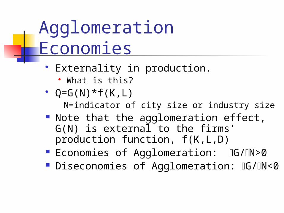
Externality in production. What is this?

Q=G(N)*f(K,L) N=indicator of city size or industry size

Note that the agglomeration effect, G(N) is external to the firms’ production function, f(K,L,D)

Economies of Agglomeration: G/N>0 Diseconomies of Agglomeration: G/N<0

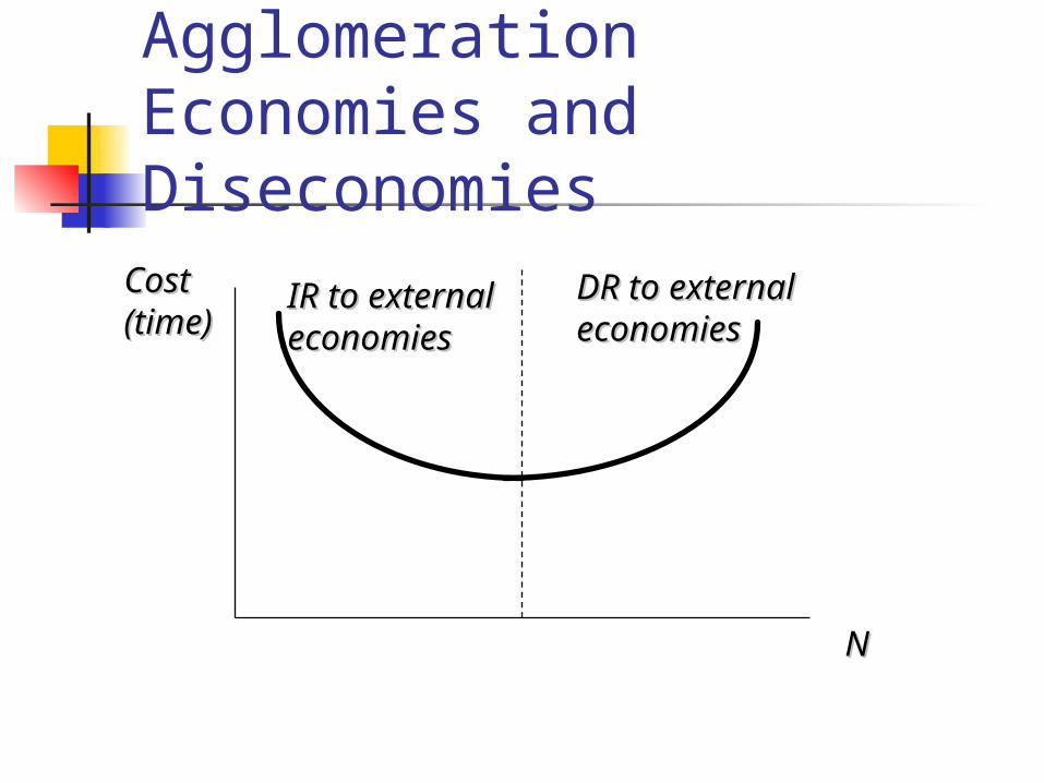
Agglomeration Economies and Diseconomies

NN

IR to externalIR to externaleconomieseconomies

DR to externalDR to externaleconomieseconomies

Cost Cost (time)(time)

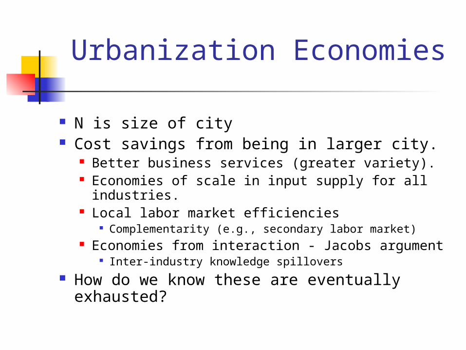
Urbanization Economies

N is size of city Cost savings from being in larger city.

Better business services (greater variety). Economies of scale in input supply for all

industries. Local labor market efficiencies

Complementarity (e.g., secondary labor market) Economies from interaction - Jacobs argument

Inter-industry knowledge spillovers How do we know these are eventually

exhausted?

Localization Economies

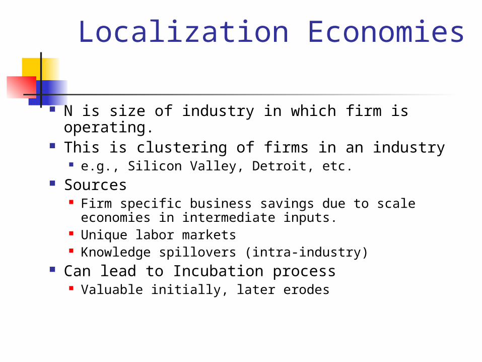
N is size of industry in which firm is operating.

This is clustering of firms in an industry e.g., Silicon Valley, Detroit, etc.

Sources Firm specific business savings due to scale

economies in intermediate inputs. Unique labor markets Knowledge spillovers (intra-industry)

Can lead to Incubation process Valuable initially, later erodes

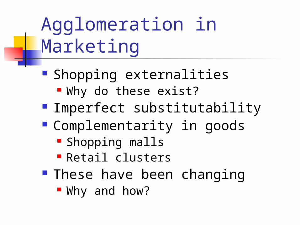
Agglomeration in Marketing Shopping externalities

Why do these exist? Imperfect substitutability Complementarity in goods

Shopping malls Retail clusters

These have been changing Why and how?

Article by Ray Vernon

Vernon looks at NYC in the late 1950’s and looks at a number of its disadvantages: No natural resource advantage high relative wages costly commuting expenses declining importance of port

Yet certain types of companies continue to locate there.

Why?

Common Characteristics

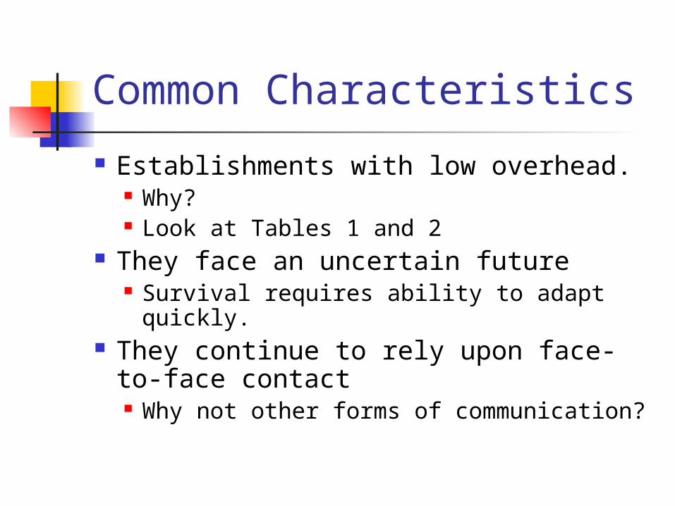
Establishments with low overhead. Why? Look at Tables 1 and 2

They face an uncertain future Survival requires ability to adapt quickly.

They continue to rely upon face-to-face contact Why not other forms of communication?

Look at some of his examples

Small dressmaking shops Rapidly changing environment. Need to meet with specialists from other

firms frequently. Military electronics

Products are unique and change rapidly. Printing

Unique jobs Publishing

Use of specialists

These are Agglomeration Economies

Urbanization or Localization?

Parallels to Corporate HQ’s

Many firms have their corporate headquarters in NYC. 156 of Fortune 500 in 1958.

They face uncertain future. Corporations need to make use of

banking, economic, financial, legal, accounting specialists.

Advantage of being near Wall Street. Need to be able to respond quickly.

Why firms leave?

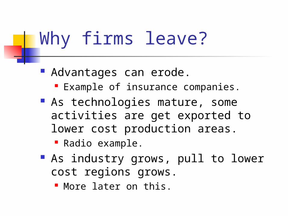
Advantages can erode. Example of insurance companies.

As technologies mature, some activities are get exported to lower cost production areas. Radio example.

As industry grows, pull to lower cost regions grows. More later on this.

Insights from article

Vernon Why look at such an old article? Insights for today? Are things changing?

Empirical Evidence on Agglomeration Economics

MSAE emphasizes empirical tools. We scratch the surface here.

Text gives other studies out there Briefly look at findings of one paper that

estimated agglomeration economies. Looked at both urbanization and localization

economics I haven’t assigned this, but for those who

are interested, the citing is: Ronald Moomaw, “Agglomeration Economies: Localization

or Urbanization: Urban Studies, 1988, Vol 25, pp. 150-161.

Overview of Moomaw

Notes that single measures of agglomeration in a production function can be misleading. Should separate urbanization and localization

economies. Classifies 2-digit manufacturing

industries according to their degree of localization (clustering near firms in same industry) and urbanization (clustering in larger urban areas).

Empirical Approach

Take a specific form of the production function. Assume specific form for urbanization and

localization economies. Manipulate this equation so that it can be

estimated. Mathematically derive a labor demand

function based on marginal productivity theory of production.

Estimate parameters of urbanization and localization.

Findings

Most urbanized industries typically have significant urbanization and/or localization economies.

Least urbanized industries have no urbanization or localization economies.

Agglomeration economies are primarily localization economies.

Some evidence of diseconomies of urbanization.

Overview of Additional Empirical Evidence John Quigley article – “Urban

Diversity and Economic Growth” reprinted from Journal of Economic Perspectives, 1998 (Vol. 12, No. 2) pp. 127-138.

Presented by Mike

History of Urbanization

Look at figure in book (2-4) Urbanization at about 7% in 1800 Urbanization at about 75% by 1990.

Variety of factors at work Rapid acceleration of Urbanization during Industrial

Revolution Agricultural Revolution Manufacturing Revolution Construction Revolution

Mr. Otis’ contribution Transportation Revolution

Inter- and intra-city All were necessary, none was sufficient to generate urbanization.

History of U.S. Urbanization:Centralization and Concentration

CentralizationCentralization DecentralizationDecentralization

19201920

ConcentrationConcentration DeconDecon ConcentrationConcentration

19701970 1980198017901790

Brief update of metro/nonmetro growth patterns for 1990’s Long and Nucci (Environment and

Planning A, 1997, Vol. 29) Show that nonmetro areas are still

growing slower than metro areas (ie., similar to most historical time periods)

However, growth in nonmetro counties is accelerating and growth in metro counties is decelerating.

Thus: Some similarities to 1970’s trend.

Reasons for Decentralization Automobile and truck have led to

suburbanization of population and employment.

Income growth and blight-flight process have reinforced the process. More later in semester.

Reasons for Deconcentration in 1970’s. Gerald Carlino evaluates this

phenomenon “Declining City Productivity and

the Growth of Rural Regions: A Test of Alternative Explanations” Journal of Urban Economics, 1985,

Vol. 18, pp. 11-27. Presented by Rose

Limiting Factors on City Growth

What factors limit size of cities? Internal scale economies Agglomeration economies Market size and transportation expenses Congestion and compensating differentials

What about the role of telecommunications? Should these strengthen or weaken pull towards

cities? Briefly review paper by Gaspar and Glaeser.

On reserve, but I have not assigned it.

Insights from Gaspar and Glaeser

“ Information Technology and the Future of Cities”, Journal of Urban Economics, 1998,Vol. 43, pp. 136-156.

Evaluates whether information technology will ultimately make it unnecessary to locate in cities

ie., move to a “spaceless world” Two opposing forces:

Substitution effect: Telecommunications innovations substitute for face-to-face meetings.

Scale effect: Telecommuncations innovations increase frequency of contact, and hence can increase demand for face-to-face meetings.

Thus: This is an empirical issue

Overview of Model Theoretical Model of Interactions:

Describes choice process whereby an individual confronted with project with expected value (ie., return) must decide:

Do this privately (without making new contacts) Do this jointly with new contacts with another person

If joint: Face-to-face (high intensity meeting) Telecommunications (low intensity meeting) Discontinue contact

Develops equilibrium conditions and then does comparative statics to evaluate impact of telecommunications advances on equilibrium

Theoretical Findings: As telecommunications improve, more

initiated contacts will lead to more exclusive telephone relationships. (Substitution effect)

As telecommunications improve, there will be more initiated contacts, since expected return from contact increases. (Scale effect)

Conclusion: If substitution effect dominates: Less need for city

locations If scale effect dominates: More need for city location

Empirical evidence Telephones and distance

U.S. evidence: In mid-1970’s, more than 40% of phone calls made to

places within 2-mile radius, and more than 75% within 6 mile radius.

Japanese evidence: #calls between 2 perfectures=f(pop, income, price,

distance) Distance coefficient is negative and significant.

Business travel Positive relationship between business travel and

telecommunications advances

Evidence - continued Co-authorship in Economics

Rising tendency over time Increases number of long-distance co-authorships,

but also local co-authorships. Cities and telephones

Japanese data shows: Minutes per household = f(income, urban status) Positive and significant coefficient on urban status (ie.,

increases telephone interactions) U.S.:

Expenditures/capita rise with city size. Historically: telephone use rises with urbanization

Conclusions Growth in telecommunications has

not diminished need for face-to-face.

Innovations in telecommunications are likely complementary, not substitutes.

What does the future hold?

Look at another article by Glaeser: “Are Cities Dying?”Journal of Economic

Perspectives, Vol. 12(2), Spring 1998, pp. 139 - 160.

Focuses on role of “agglomerating” vs. “congesting” forces and discusses which are likely to dominate

Presented by: Joe

Dorian Friedman – U.S. News and World Report article Suggests that Downtown regions are

experiencing some type of renaissance. Sparked by downtown construction of

entertainment facilities Inmigration of empty-nesters Growth of cultural attractions

Is this consistent with other perspectives? What type of agglomeration is emphasized

here? Do you think this is happening?

The Economist Article Focuses on the revitalization of Chicago’s

State Street “Transit mall” experiment scrapped Through-traffic re-introduced Role of demographics

Empty-nesters (young and old) Attraction of retailers (more later in

semester) Role of TIF districts

Some controversy Conclusion

Role of Comparative Advantage

We now understand why cities exist Internal Scale Economies External Economies or Agglomeration

Effects Can be Localization and/or Urbanization

Now we turn to models of where cities evolve Will consider both the locational choices of

people and firms. Two sides of labor market as well as retirees.

Comparative Advantage and Location of Cities Look at cost-minimizing behavior

of firms in context of model where friction of space is introduced.

Comparative Advantage: A firm can produce a product at lower

opportunity cost than firms in other regions.

Explains why regions specialize.

There are Two Types of Firms

Transfer Orientation Geographic differences in

transport costs are more important than geographic differences in other costs.

Cost of transportation of raw materials vis a vis finished product is driving force.

Examples include steel, autos, beer.

Local Input Cost Orientation

Geographic differences in other inputs (labor, land, capital, energy, amenities) more important than transport costs.

Pull of non-transport factors is driving force.

Examples include textiles, computers, R&D

Transfer-Oriented Production Firms

Start with very simple assumptions and later relax them.

Assume firm produces single output, sold at single point (market=M) and uses raw materials from single source (Forest=F).

Only one input needs to be transported. All others are ubiquitous.

There is a comparative advantage for the input at F, and it is not available elsewhere.

Assumptions - continued

Firm does not substitute among inputs (fixed proportions).

Firm is small in relation to input and output markets.

Transport costs are constant/mile at t.

There is single mode of transport.

Total Transport Costs

Total Transport Costs Total Transport Costs

F MTotal Distance = xm

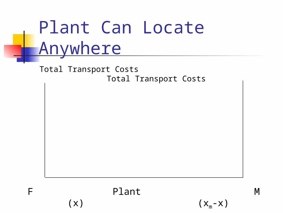
Plant Can Locate AnywhereTotal Transport Costs Total

Transport Costs

F Plant M (x) (xm-x)

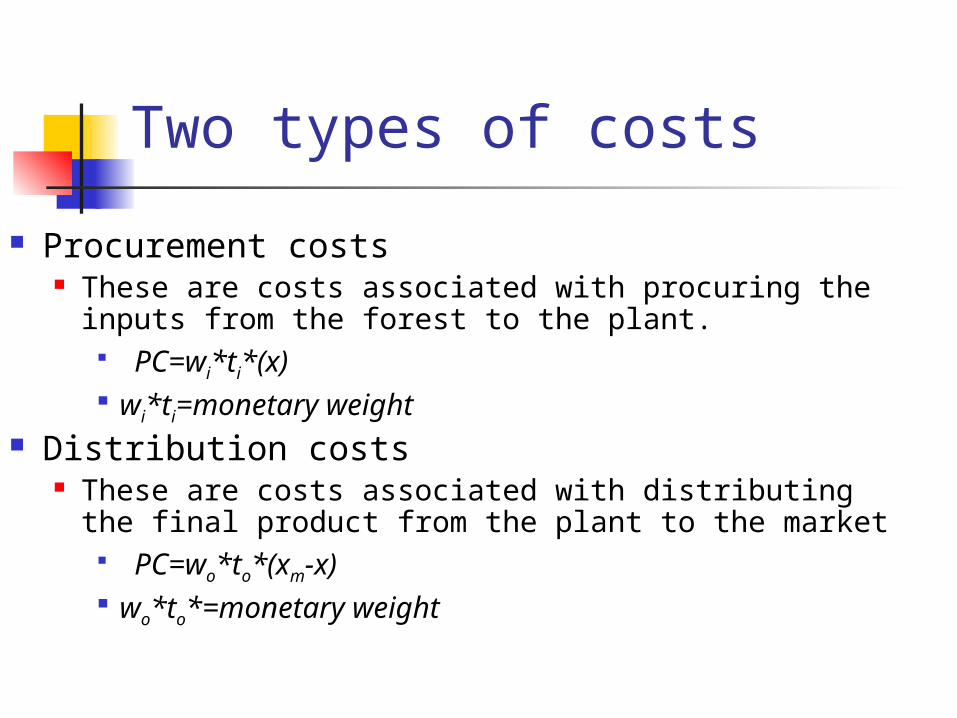
Two types of costs

Procurement costs These are costs associated with procuring the

inputs from the forest to the plant. PC=wi*ti*(x) wi*ti=monetary weight

Distribution costs These are costs associated with distributing the

final product from the plant to the market PC=wo*to*(xm-x) wo*to*=monetary weight

Procurement Costs

Procurement Costs Procurement Costs

F M

slope= wwii*t*tii

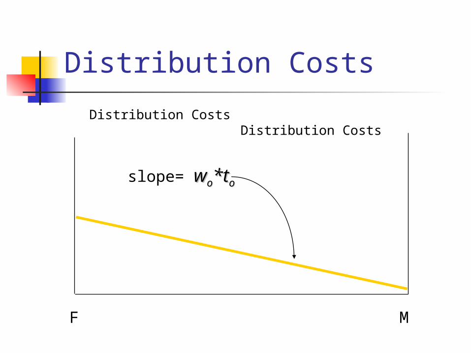
Distribution Costs

Distribution Costs Distribution Costs

F M

slope= wwoo*t*too

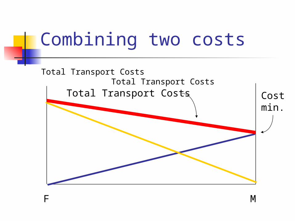
Combining two costs

Total Transport Costs Total Transport Costs

F M

Total Transport Costs Costmin.

Question: What determines the optimal

location

Compare the monetary weights of the inputs and

the output.

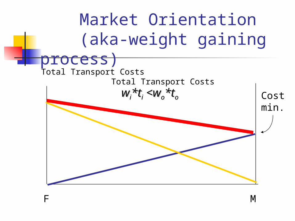
Market Orientation (aka-weight gaining process)Total Transport Costs Total

Transport Costs

F M

Costmin.

wwii*t*tii <w <woo*t*too

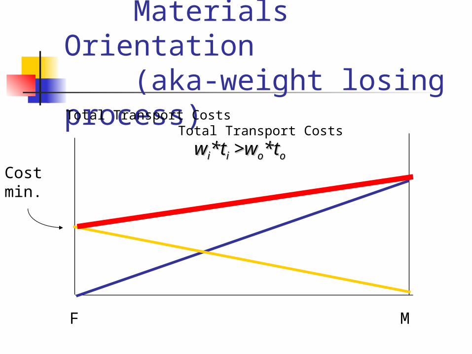
Materials Orientation (aka-weight losing process)Total Transport Costs Total

Transport Costs

F M

Costmin.

wwii*t*tii >w >woo*t*too

Why do we always get endpoint solutions?

Because monetary weights are constants.

Adding realism

Terminal costs are costs associated with loading and unloading These increase if you locate at

intermediate locations. Nonconstant values for ti and to.

we expect t falls with distance shipped. Look at implications for our model

Transport Costs function of distance

Total Transport Costs Total Transport Costs

F M

Total Transport CostsCostmin.

Adding in Terminal Costs

Total Transport Costs Total Transport Costs

F M

Costmin.

T

Question: Does realism increase or decrease the likelihood of an endpoint

solution?

Allow multiple markets

Assume inputs are all ubiquitous. Keep simple assumptions of constant transport

costs. If transportation costs are important, then firms

will choose Median location Assume each input weighs 1 lb. and transport

costs per mile are $2.00. Monetary weight per customer=wo*to=1*2=2

Assume markets are 1 mile apart.

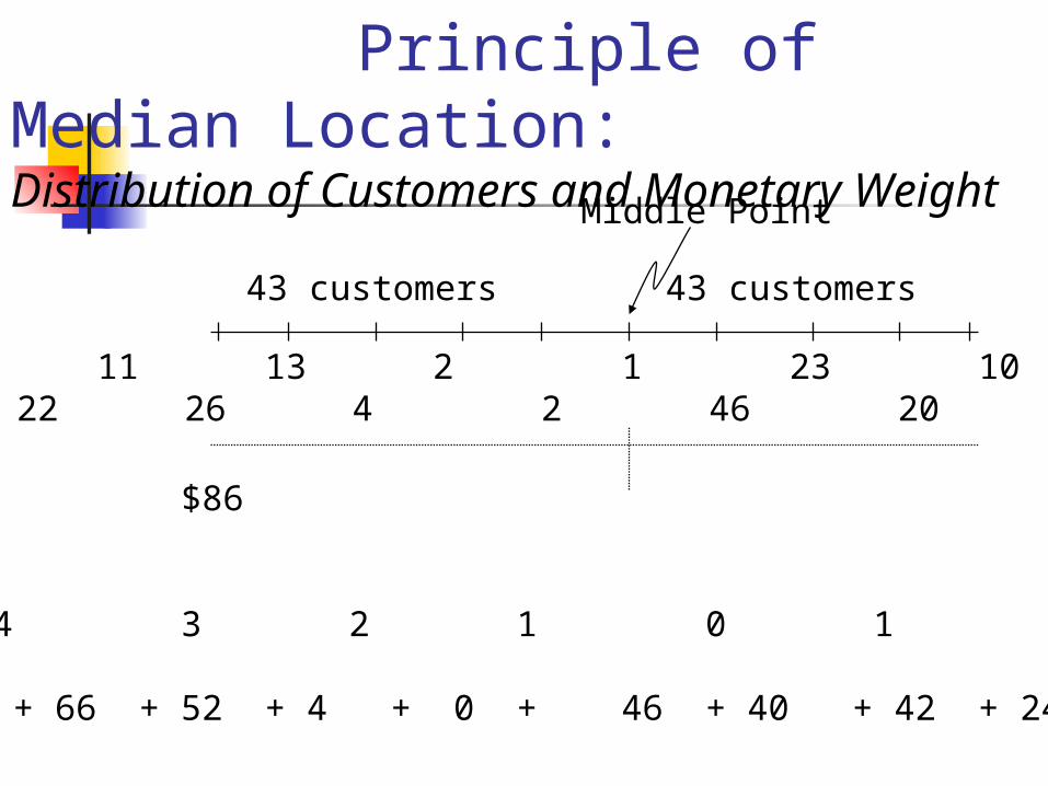
Principle of Median Location:Distribution of Customers and Monetary Weight

Customers: 8 9 11 13 2 1 23 10 7 3MW=wo*to: 16 18 22 26 4 2 46 20 14 6

Sum of MW: $86 $86

Miles frommidpoint: 5 4 3 2 1 0 1 2 3 4

Total Costs:80 + 72 + 66 + 52 + 4 + 0 + 46 + 40 + 42 + 24= $426

Middle Point

43 customers 43 customers

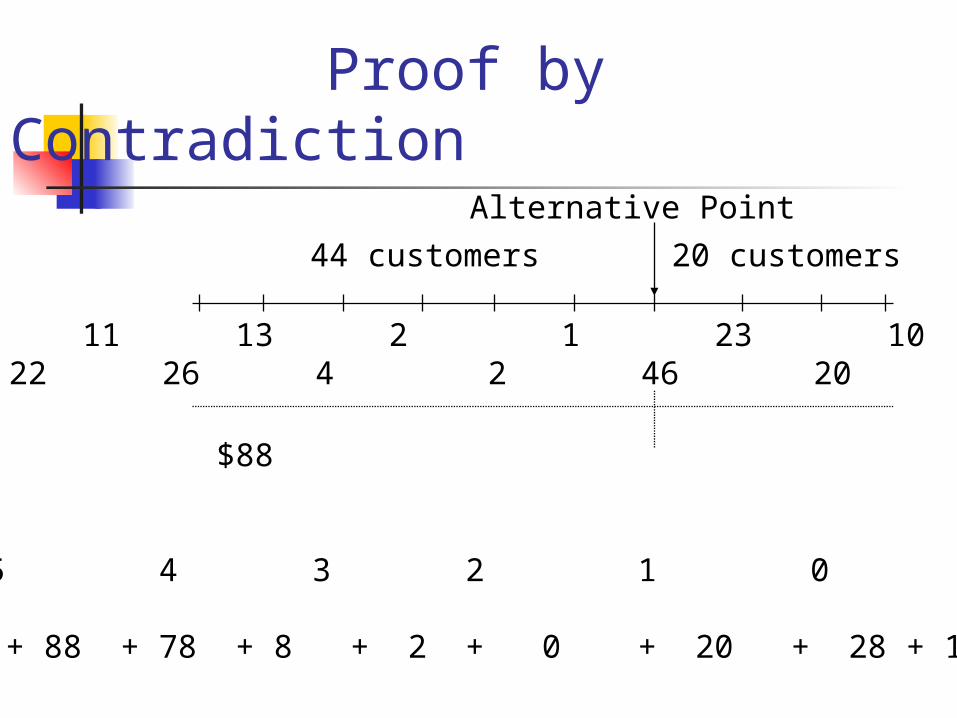
Proof by Contradiction

Customers: 8 9 11 13 2 1 23 10 7 3MW=wo*to: 16 18 22 26 4 2 46 20 14 6

Sum of MW: $88 $40

Miles frommidpoint: 6 5 4 3 2 1 0 1 2 3

Total Costs:96 + 90 + 88 + 78 + 8 + 2 + 0 + 20 + 28 + 18= $428

Alternative Point

44 customers 20 customers

Question: Why does this happen?

Other Input Cost Orientations

Other types of costs may matter more to firms. These include: Labor Orientation

Amenity Orientation Energy Orientation Land Orientation External Economy Orientation Fiscal Orientation

Graphical depiction

Suppose that one location has lower labor costs than another. e.g., South has more right to work laws, and

lower unionization rates. We can adapt our most simple model. Look at balancing of labor and transport

costs. Assume one kind of transport costs. Assume labor costs decline with distance.

Labor Oriented Firm

Transport+Labor Costs Transport+Labor Costs

M Low cost Labor

Costmin.

DistributionCosts

Labor Costs

MinimumLabor Costs

Two types of Orientations

What have we observed over time? Transport costs have continually declined. Reasons:

Lighter materials More efficient transport modes

Container systems on ships Deregulation of trucking Development of interstate highway system

Internationalization of markets generating other input cost differentials.

Next time - Look at Firm Location and Household Location Decisions

Firm Location Bartik – Clark will do this one Leichenko

Household Location Clark and Hunter

Broad Regional Trends Chinitz