UQTk - A C++/Python Toolkit for Uncertainty Quantificationneckel/siamuq16_slides_minisymp/2016_uqtk... · A C++/Python Toolkit for Uncertainty Quantiﬁcation ... Part of US DOE BER

Intro Workflow Summary References

UQTkA C++/Python Toolkit for Uncertainty Quantification

Bert Debusschere, Khachik Sargsyan, Cosmin Safta,Kenny Chowdhary

[email protected] National Laboratories,

Livermore, CA, USA

Wed April 6, 2016 – SIAM UQ 16

Debusschere – SNL UQTk


Acknowledgements

Cosmin Safta Sandia National LaboratoriesKhachik Sargsyan Livermore, CA, USAKenny ChowdharyHabib NajmOmar Knio Duke University, Raleigh, NC, USARoger Ghanem University of Southern California

Los Angeles, CA, USAOlivier Le Maître LIMSI-CNRS, Orsay, Franceand many others ...

This material is based upon work supported by the U.S. Department of Energy, Officeof Science, Office of Advanced Scientific Computing Research (ASCR), ScientificDiscovery through Advanced Computing (SciDAC) and Applied Mathematics Research(AMR) programs.

Sandia National Laboratories is a multi-program laboratory managed and operated bySandia Corporation, a wholly owned subsidiary of Lockheed Martin Corporation, for theU.S. Department of Energy’s National Nuclear Security Administration under contractDE-AC04-94AL85000.



Outline

1 General Characteristics

2 An Example Workflow

3 Summary

4 References



UQ is about enabling predictive simulations

Predictive Simulation

Theory

Experiments



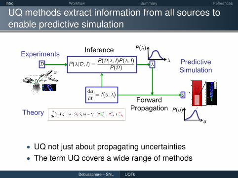
UQ methods extract information from all sources toenable predictive simulation

Predictive Simulation

Theory

Experiments

Introduction Introduction UQ Software PCES Summary References

Formulation

dudt

= f (u;λ)

P(λ|D, I) =P(D|λ, I)p(λ, I)

P(D)

Debusschere – SNL UQ


Formulation

dudt

= f (u;λ)


P(D)



Formulation

dudt

= f (u;λ)


P(D)



Formulation

dudt

= f (u;λ)


P(D)


Inference

Forward Propagation


Formulation

dudt

= f (u;λ)

P(λ|D, I) =P(D|λ, I)P(λ, I)

P(D)

λ u

P(u) P(λ)



Formulation

dudt

= f (u;λ)


P(D)

λ u

P(u) P(λ)



Formulation

dudt

= f (u;λ)


P(D)

λ u

P(u) P(λ)



Formulation

dudt

= f (u;λ)


P(D)

λ u

P(u) P(λ)



Formulation

dudt

= f (u;λ)


P(D)

λ u

P(u) P(λ)

Debusschere – SNL UQ• UQ not just about propagating uncertainties• The term UQ covers a wide range of methods



UQTk provides tools to build a general UQ workflow

• Tools for• Representation of random variables and stochastic

processes• Forward uncertainty propagation• Inverse problems• Sensitivity analysis• Bayesian Compressive Sensing• Gaussian Processes

• Tools can be used stand-alone or combined into ageneral workflow



We want UQTk to be straightforward to download,install and use

• Target usage:• Rapid prototyping of UQ workflows• Algorithmic research in UQ• Tutorials / educational

• Released under the GNU Lesser General PublicLicense• http://www.sandia.gov/UQToolkit/

• Current version 2.1• Version 3.0 coming (very) soon

• No massive third party libaries to download, install,and configure


http://www.sandia.gov/UQToolkit/


UQTk is used in a variety of applications

• Direct collaborations• US DOE SciDAC QUEST UQ institutehttp://www.quest-scidac.org

• Variety of US DOE SciDAC partnership projects• Part of US DOE BER ACME climate model analysis

tools• Always welcome new applications / collaborations

• Downloads from http://www.sandia.gov/UQToolkit

• ≈ 600 total downloads• ≈ 425 downloads of version 2.x• Mostly academic and laboratory research groups

• Mailing lists• [email protected]• [email protected]• Join at http://www.sandia.gov/UQToolkit


http://www.quest-scidac.org

http://www.sandia.gov/UQToolkit

[email protected]

[email protected]



We rely on Polynomial Chaos expansions (PCEs) torepresent uncertainty

• Standard PC Basis types supported:• Gauss – Hermite• Uniform – Legendre• Gamma – Laguerre• Beta – Jacobi

• Also support for custom orthogonal polynomials• Defined by user-provided three-term recurrence

formula• Both intrusive and non-intrusive PC tools provided

• Primarily Galerkin projection methods• Some regression approaches offered through

Bayesian Compressed Sensing module• See also Debusschere, et al. 2004; Sargsyan, et al.

2014Debusschere – SNL UQTk


UQTk uses a combination of C++ and Python

• Main libraries in C++• PCBasis and PCSet classes: PC tools (intrusive and

non-intrusive)• Quad class: quadrature rules (full tensor and sparse

tensor product rules)• MCMC, Gproc, . . .

• Functionality available via• Direct linking of C++ code• Standalone apps• Python interface based on Swig (UQTk version 3.0)

• Download as tar file and configure with CMake

• Examples of common workflows provided



Outline

1 General Characteristics

2 An Example Workflow

3 Summary

4 References



An example UQTk workflow (UQTk version 3.0)

Forward UQ

Inverse UQ

f(λ)

Model

fc(λ)

Surrogate

Dim.Red.

Likelihood D = {yi}

Data

Posterior p(λ|D)

Prior p(λ)

g(λ)

Any model

Prediction p(g(λ)|D)



An example UQTk workflow (UQTk version 3.0)

• Consider uncertain parameter vector λ• Propagate uncertainty in λ through model g(λ)• First calibrate λ using data on function f (λ)• Consider the following calibration functions f (λ):

• Gaussian: f G(λ) = exp(−∑d

i=1 a2i λ

2i

)• Exponential: f E(λ) = exp

(∑di=1 aiλi

)• 5 dimensional λ: a = (0.4,0.3,0.2,0.1,0.05)

• Forward models g(λ):• Gaussian: g1(λ) = f G(λ)• Exponential: g2(λ) = f E(λ)• Summation: g3(λ) =

∑di=1 λi

• For more details, see “Handbook of UncertaintyQuantification", Springer, 2016



Surrogate models provide computationally cheapapproximations for full forward model

• Used instead of full forward model in computationallydemanding operations such as optimization andcalibration

• Use PCE surrogate model• Same approach as forward UQ

• Legendre-Uniform PCEs• Use uniform distributions over range of input

parameters• Galerkin projection with Gauss quadrature• 3rd order PCE using 45 = 1024 quadrature points• 111 random validation samples to assess surrogate

accuracy



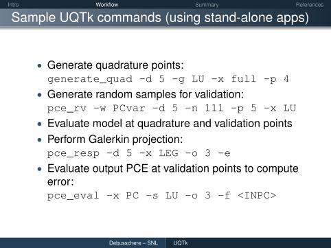
Sample UQTk commands (using stand-alone apps)

• Generate quadrature points:generate_quad -d 5 -g LU -x full -p 4

• Generate random samples for validation:pce_rv -w PCvar -d 5 -n 111 -p 5 -x LU

• Evaluate model at quadrature and validation points• Perform Galerkin projection:pce_resp -d 5 -x LEG -o 3 -e

• Evaluate output PCE at validation points to computeerror:pce_eval -x PC -s LU -o 3 -f <INPC>



Surrogate Construction

Gaussian

0.75 0.80 0.85 0.90 0.95 1.00 1.05Model

0.75

0.80

0.85

0.90

0.95

1.00

1.05

Polynomial Surrogate

training points

validation points

y=x

Exponential

0.5 1.0 1.5 2.0Model

0.5

1.0

1.5

2.0

Polynomial Surrogate

training points

validation points

y=x

• 3rd order PC surrogate accurate up to 0.1% relativeerror for both Gaussian and Exponential function



Sensitivity analysis enables dimensionality reduction

• UQTk computes main, joint, and total sensitivitycoefficients• Si : Fraction of variance due to λi only• Sij : Fraction of variance due to both λi and λj• ST

i : Fraction of variance due to λi by itself and incombination with any other λj

• Can be computed analytically from PC responsesurface

• pce_sens -m mindex.dat \-f PCcoeff_quad.dat -x LU



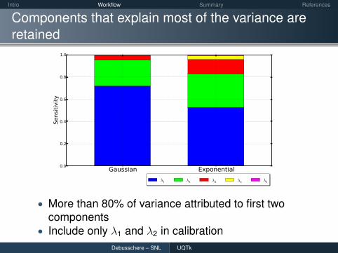
Components that explain most of the variance areretained

Gaussian Exponential0.0

0.2

0.4

0.6

0.8

1.0Sensitivity

λ1 λ2 λ3 λ4 λ5

• More than 80% of variance attributed to first twocomponents

• Include only λ1 and λ2 in calibrationDebusschere – SNL UQTk


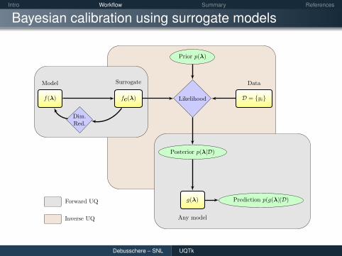
Bayesian calibration using surrogate models

Forward UQ

Inverse UQ

f(λ)

Model

fc(λ)

Surrogate

Dim.Red.

Likelihood D = {yi}

Data

Posterior p(λ|D)

Prior p(λ)

g(λ)

Any model




Bayesian Parameter Inference

Posterior︷︸︸︷p(λ|D) ∝

Likelihood︷︸︸︷p(D|λ)

Prior︷︸︸︷p(λ)

LD(λ) = p(D|λ) ∝R∏

j=1

exp

(−(yG

j − f G(λ))2

2σ2

)exp

(−(yE

j − f E(λ))2

2σ2

)

• Generate R random noisy realizations of f G(λ) andf E(λ) as data D

• Assume Normally distributed priors N(0,0.3) on λ1

and λ2

• Infer λ1 and λ2 against data on both f G(λ) and f E(λ)• model_inf -x xfile.dat -y yfile.dat -f pc \

-l classical -m 100000 -e 0.01 -i normal



Markov Chain Monte Carlo generates a set ofposterior samples

λ1

0 20000 40000 60000 80000 100000MCMC Sample

−1.0

−0.8

−0.6

−0.4

−0.2

0.0

0.2

Parameter λ1

λ2

0 20000 40000 60000 80000 100000MCMC Sample

−1.5

−1.0

−0.5

0.0

0.5

1.0

Parameter λ2

• The chains for both parameters show good mixing



Marginal and Joint Posterior Densities

0.0

0.5

1.0

1.5

2.0

2.5

3.0λ1

PDF of λ1

−1.0 −0.5 0.0 0.5λ2

0.0

0.5

1.0

1.5

2.0PDF of λ2

−0.8 −0.6 −0.4 −0.2 0.0λ1

−1.0

−0.5

0.0

0.5

λ2



Forward propagation with calibrated parameters

Forward UQ

Inverse UQ

f(λ)

Model

fc(λ)

Surrogate

Dim.Red.

Likelihood D = {yi}

Data

Posterior p(λ|D)

Prior p(λ)

g(λ)

Any model




The Rosenblatt transformation maps the posteriorsamples to standard Gaussian random variables

• Posterior distributions represent the parameteruncertainties

• Set of MCMC samples characterizes these posteriors• Need to project these posteriors onto Gauss-Hermite

PC basis to get PCE for λ• Galerkin projection requires map between posterior

samples and ξ• Rosenblatt transformation provides this mapping• pce_quad provides this map to project samples onto

PCEs



Rosenblatt mapping of quadrature points enablesGalerkin projection onto Gauss-Hermite basis

−0.8 −0.7 −0.6 −0.5 −0.4 −0.3 −0.2 −0.1 0.0Parameter λ1

−1.0

−0.8

−0.6

−0.4

−0.2

0.0

Parameter λ2

MCMC samples

Quadrature samples

λ1 =P∑

k=0

λ1k Ψk (ξ) λ1k ∝∫

R−1λ1

(ξ)︸︷︷︸λ1

Ψk (ξ)w(ξ)dξ

λ2 =P∑

k=0

λ2k Ψk (ξ) λ2k ∝∫

R−1λ2

(ξ)︸︷︷︸λ2

Ψk (ξ)w(ξ)dξ



Forward propagation uses similar commands assurrogate construction

• Use calibrated uncertainty on λ1, λ2

• Keep prior uncertainty N(0,0.3) on λ3, λ4, λ5

• Forward models g(λ):• Gaussian: g1(λ) = f G(λ)• Exponential: g2(λ) = f E(λ)• Summation: g3(λ) =

∑di=1 λi

• Quadrature Galerkin projection• generate_quad -d 5 -g HG -x full -p 4• Evaluate model at quadrature points• pce_resp -d 5 -x HG -o 3



Input calibration reduces output uncertainty

0.86 0.88 0.90 0.92 0.94 0.96 0.98 1.00Model Output

0

10

20

30

40

50

60

PDF

Gaussian

Prior

Posterior

0.4 0.6 0.8 1.0 1.2 1.4 1.6 1.8 2.0Model Output

0

1

2

3

4

5

6

7

8

PDF

Exponential

Prior

Posterior

• After calibration: output distributions narrow and shift



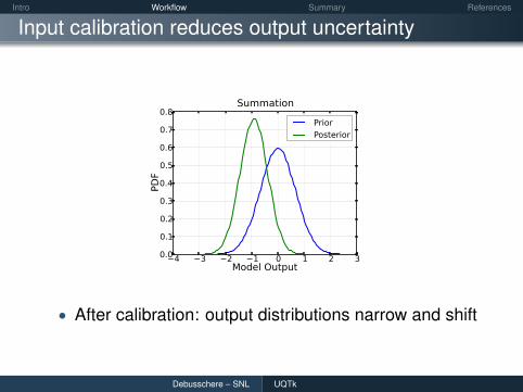
Input calibration reduces output uncertainty

−4 −3 −2 −1 0 1 2 3Model Output

0.0

0.1

0.2

0.3

0.4

0.5

0.6

0.7

0.8

PDF

Summation

Prior

Posterior

• After calibration: output distributions narrow and shift



Attribution relates output uncertainties to specificinputs

Gaussian Exponential Summation0.0

0.2

0.4

0.6

0.8

1.0

Sensitivity

(λ1 ,λ2 ) λ3 λ4 λ5

• Attribution uses sensitivity analysis tools: pce_sens• For Gaussian model: more data needed to further

reduce input uncertainty in λ1, λ2

• For other two models, need to calibrate other inputsDebusschere – SNL UQTk


Summary

• UQTk provides a powerful set of tools for buildinggeneral UQ workflows

• Multiple ways to access functionality• Direct linking of C++ code• Standalone apps• Python interface based on Swig (UQTk version 3.0)

• Version 3.0 soon athttp://www.sandia.gov/UQToolkit

• Do not hesitate to contact [email protected]



[email protected]


References

• B. Debusschere, H. Najm, P. Pébay, O. Knio, R.Ghanem and O. Le Maître, “Numerical Challenges inthe Use of Polynomial Chaos Representations forStochastic Processes", SIAM J. Sci. Comp., 26:2,2004.

• K. Sargsyan, et al., “Dimensionality reduction forcomplex models via bayesian compressive sensing",Int. J. of Uncertainty Quantification, 4, 1:63-93, 2014.

• “Handbook of Uncertainty Quantification", R.Ghanem, D. Higdon, H. Owhadi (Eds.), Springer,2016, http://www.springer.com/us/book/9783319123844

• UQ Tutorials: http://www.quest-scidac.org/outreach/tutorials/


http://www.springer.com/us/book/9783319123844

http://www.springer.com/us/book/9783319123844

http://www.quest-scidac.org/outreach/tutorials/

http://www.quest-scidac.org/outreach/tutorials/


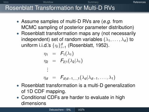
Rosenblatt Transformation for Multi-D RVs

• Assume samples of multi-D RVs are (e.g. fromMCMC sampling of posterior parameter distribution)

• Rosenblatt transformation maps any (not necessarilyindependent) set of random variables (λ1, . . . , λd) touniform i.i.d.’s {ηi}d

i=1 (Rosenblatt, 1952).

η1 = F1(λ1)

η2 = F2|1(λ2|λ1)

...ηd = Fd |d−1,...,1(λd |λd−1, . . . , λ1)

• Rosenblatt transformation is a multi-D generalizationof 1D CDF mapping.

• Conditional CDFs are harder to evaluate in highdimensions


Documents

UQTk - A C++/Python Toolkit for Uncertainty Quantificationneckel/siamuq16_slides_minisymp/2016_uqtk... · A C++/Python Toolkit for Uncertainty Quantiﬁcation ... Part of US DOE BER